System Identification and Control of aPolymer Reactor

Tobias Munker ∗ Geritt Kampmann ∗ Max Schussler ∗

Oliver Nelles ∗

∗ Automatic Control - Mechatronics, University of Siegen, Germany(e-mail: tobias.muenker@uni-siegen.de).

Abstract: In a polymer production process, a special reactor is used to adjust the viscosity,i.e., chain length of the polymer. This reactor has several control variables mainly in manuallycontrol. For future automatic control concepts, such a reactor is modeled from data with alinear (regularized FIR) and a nonlinear state space model (LMSSN). A model predictive controlapproach is presented in simulation.

Keywords: Reactor control, regularized FIR model, local model state space network (LMSSN),model predictive control (MPC), nonlinear dynamic model, system identification

1. INTRODUCTION

Nowadays, production plants collect vast amounts of pro-cess data during production time. Often this data isrecorded, and there is an intention to use it for improve-ments in product quality. This contribution presents asystem-based approach for the identification and controlof a chemical process. Therefore first, a model is identifiedand second, a suitable controller for viscosity is developedbased on the identified model.

The process data used for this study stems from a contin-uous polymer reactor (PR) equipped with two horizontalagitators. This finishing reactor is used to increase theviscosity of the feed to the desired target. The viscositycorresponds to the mean chain length of the polymerand is one of the key quality figures. Viscosity is mainlycontrolled by pressure and agitator speed besides other pa-rameters as throughput, catalyst, and temperature. Thesecontrol parameters are set manually by the plant opera-tors, potentially supported by a viscosity controller actingon the pressure.

The goal of this study is to apply modern techniques fromcontrol and identification to improve this situation. In thefirst step, a novel approach for regularized linear systemidentification, introduced by Pillonetto et al. (2010), isused to derive a data-based model. In this approach aregularized estimate of the parameters for a finite impulseresponse model is obtained, see Chen et al. (2012). It hasbeen shown by Pillonetto et al. (2014) in extensive simula-tion studies that for the identification of dynamic systems,this approach performs favorably. The identification of alinear model allows a thorough system analysis and theuse of powerful control techniques. It can be seen thatthe system has a non-minimum phase behavior. Based onthis observation, two control schemes are developed andcompared. On the one hand, a classical PI-control is tunedwith the identified model. On the other hand, a modelpredictive control (MPC) scheme, see Camacho and Alba(2007), is investigated.

In Sect. 2 both the linear and the nonlinear approach foridentification of the plant are described. In Sect. 3 thebehavior of the plant is analyzed and two control schemes,one PI control scheme, and a model predictive approachare presented. Section 4 concludes the paper.

2. SYSTEM IDENTIFICATION

The process and the obtained data are described first.Then, the modeling approaches for the linear and non-linear cases are introduced.

2.1 Process Inputs and Output

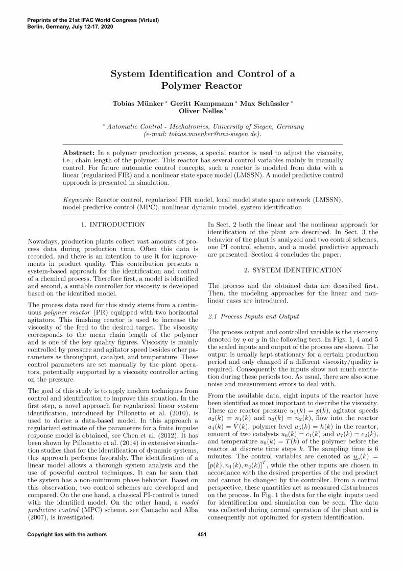
The process output and controlled variable is the viscositydenoted by η or y in the following text. In Figs. 1, 4 and 5the scaled inputs and output of the process are shown. Theoutput is usually kept stationary for a certain productionperiod and only changed if a different viscosity/quality isrequired. Consequently the inputs show not much excita-tion during these periods too. As usual, there are also somenoise and measurement errors to deal with.

From the available data, eight inputs of the reactor havebeen identified as most important to describe the viscosity.These are reactor pressure u1(k) = p(k), agitator speedsu2(k) = n1(k) and u3(k) = n2(k), flow into the reactor

u4(k) = V (k), polymer level u5(k) = h(k) in the reactor,amount of two catalysts u6(k) = c1(k) and u7(k) = c2(k),and temperature u8(k) = T (k) of the polymer before thereactor at discrete time steps k. The sampling time is 6minutes. The control variables are denoted as uc(k) =

[p(k), n1(k), n2(k)]T

, while the other inputs are chosen inaccordance with the desired properties of the end productand cannot be changed by the controller. From a controlperspective, these quantities act as measured disturbanceson the process. In Fig. 1 the data for the eight inputs usedfor identification and simulation can be seen. The datawas collected during normal operation of the plant and isconsequently not optimized for system identification.

Preprints of the 21st IFAC World Congress (Virtual)Berlin, Germany, July 12-17, 2020

Copyright lies with the authors 451

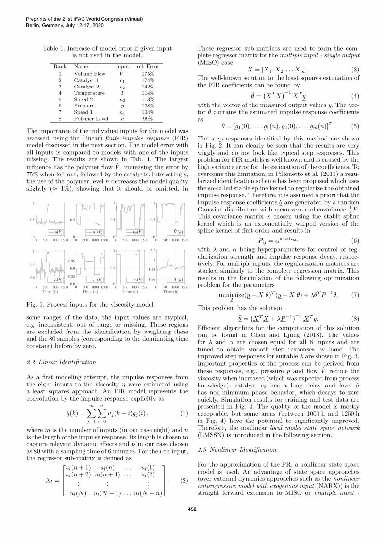
Table 1. Increase of model error if given inputis not used in the model.

Rank Name Input rel. Error

1 Volume Flow V 175%2 Catalyst 1 c1 174%3 Catalyst 2 c2 142%4 Temperature T 114%5 Speed 2 n2 113%6 Pressure p 108%7 Speed 1 n1 104%8 Polymer Level h 99%

The importance of the individual inputs for the model wasassessed, using the (linear) finite impulse response (FIR)model discussed in the next section. The model error withall inputs is compared to models with one of the inputsmissing. The results are shown in Tab. 1. The largestinfluence has the polymer flow V , increasing the error by75% when left out, followed by the catalysts. Interestingly,the use of the polymer level h decreases the model qualityslightly (≈ 1%), showing that it should be omitted. In

0 500 1000 15000

0.5

1

0 500 1000 15000

0.5

1

0 500 1000 15000

0.5

1

0 500 1000 15000

0.5

1

0 500 1000 1500

0.6

0.8

1

0 500 1000 15000.8

0.85

0.9

0.95

1

0 500 1000 15000

0.5

1

0 500 1000 1500

0.96

0.98

1

1.02

Fig. 1. Process inputs for the viscosity model.

some ranges of the data, the input values are atypical,e.g. inconsistent, out of range or missing. These regionsare excluded from the identification by weighting theseand the 80 samples (corresponding to the dominating timeconstant) before by zero.

2.2 Linear Identification

As a first modeling attempt, the impulse responses fromthe eight inputs to the viscosity η were estimated usinga least squares approach. An FIR model represents theconvolution by the impulse response explicitly as

y(k) =

m∑

j=1

n∑

i=0

uj(k − i)gj(i) , (1)

where m is the number of inputs (in our case eight) and nis the length of the impulse response. Its length is chosen tocapture relevant dynamic effects and is in our case chosenas 80 with a sampling time of 6 minutes. For the l-th input,the regressor sub-matrix is defined as

Xl =

ul(n+ 1) ul(n) . . . ul(1)ul(n+ 2) ul(n+ 1) . . . ul(2)

......

...ul(N) ul(N − 1) . . . ul(N − n)

. (2)

These regressor sub-matrices are used to form the com-plete regressor matrix for the multiple input - single output(MISO) case

X = [X1 X2 . . . Xm] . (3)

The well-known solution to the least squares estimation ofthe FIR coefficients can be found by

θ =(XTX

)−1XT y (4)

with the vector of the measured output values y. The vec-tor θ contains the estimated impulse response coefficientsas

θ = [g1(0), . . . , g1(n), g2(0), . . . , gm(n)]T. (5)

The step responses identified by this method are shownin Fig. 2. It can clearly be seen that the results are verywiggly and do not look like typical step responses. Thisproblem for FIR models is well known and is caused by thehigh variance error for the estimation of the coefficients. Toovercome this limitation, in Pillonetto et al. (2011) a regu-larized identification scheme has been proposed which usesthe so-called stable spline kernel to regularize the obtainedimpulse response. Therefore, it is assumed a priori that theimpulse response coefficients θ are generated by a randomGaussian distribution with mean zero and covariance 1

λP .This covariance matrix is chosen using the stable splinekernel which is an exponentially warped version of thespline kernel of first order and results in

Pij = αmax(i,j) (6)

with λ and α being hyperparameters for control of reg-ularization strength and impulse response decay, respec-tively. For multiple inputs, the regularization matrices arestacked similarly to the complete regression matrix. Thisresults in the formulation of the following optimizationproblem for the parameters

minimizeθ

(y −X θ)T (y −X θ) + λθTP−1θ. (7)

This problem has the solution

θ =(XTX + λP−1

)−1XT y. (8)

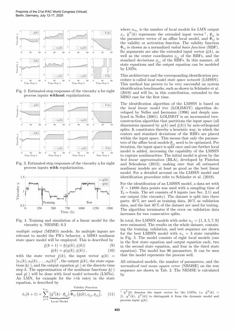
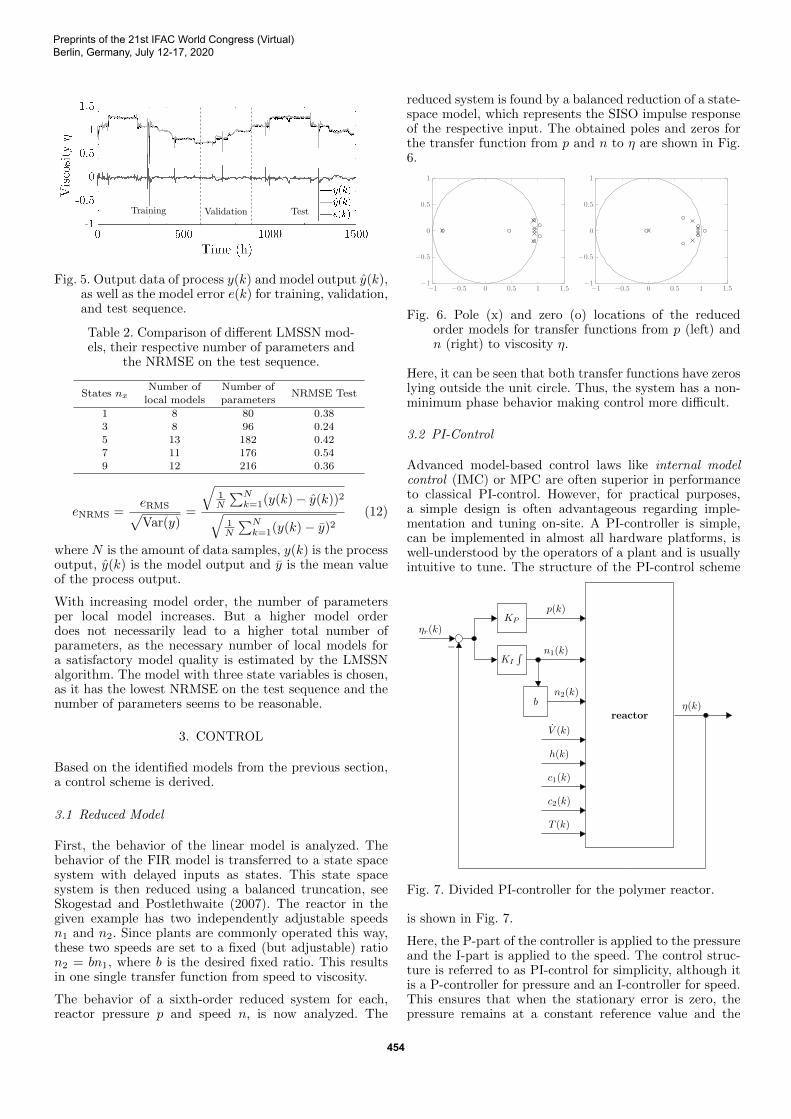
Efficient algorithms for the computation of this solutioncan be found in Chen and Ljung (2013). The valuesfor λ and α are chosen equal for all 8 inputs and aretuned to obtain smooth step responses by hand. Theimproved step responses for suitable λ are shown in Fig. 3.Important properties of the process can be derived fromthese responses, e.g., pressure p and flow V reduce theviscosity when increased (which was expected from processknowledge), catalyst c2 has a long delay and level hhas non-minimum phase behavior, which decays to zeroquickly. Simulation results for training and test data arepresented in Fig. 4. The quality of the model is mostlyacceptable, but some areas (between 1000 h and 1250 hin Fig. 4) have the potential to significantly improved.Therefore, the nonlinear local model state space network(LMSSN) is introduced in the following section.

2.3 Nonlinear Identification

For the approximation of the PR, a nonlinear state spacemodel is used. An advantage of state space approaches(over external dynamics approaches such as the nonlinearautoregressive model with exogenous input (NARX)) is thestraight forward extension to MISO or multiple input -

Preprints of the 21st IFAC World Congress (Virtual)Berlin, Germany, July 12-17, 2020

452

-1

0

1

0 40 80

-1

0

1

0 40 80

-1

0

1

0 40 80

-1

0

1

0 40 80

-1

0

1

0 40 80

-1

0

1

0 40 80

-1

0

1

0 40 80

-1

0

1

0 40 80

Fig. 2. Estimated step responses of the viscosity η for eightprocess inputs without regularization.

-1

0

1

0 40 80

-1

0

1

0 40 80

-1

0

1

0 40 80

-1

0

1

0 40 80

-1

0

1

0 40 80

-1

0

1

0 40 80

-1

0

1

0 40 80

-1

0

1

0 40 80

Fig. 3. Estimated step responses of the viscosity η for eightprocess inputs with regularization.

0 250 500 750 1000 1250 15000.5

1

1.5

Fig. 4. Training and simulation of a linear model for theviscosity η. NRMSE: 0.3

multiple output (MIMO) models. As multiple inputs arerelevant to model the PR’s behavior, a MISO nonlinearstate space model will be employed. This is described by

x(k + 1) = h(u(k), x(k)) (9)

y(k) = g(u(k), x(k)) , (10)

with the state vector x(k), the input vector u(k) =

[u1(k), u2(k), . . . , u8(k)]T

, the output y(k), the state equa-tions h(·), and the output equation g(·) at the discrete timestep k. The approximation of the nonlinear functions h(·)and g(·) will be done with local model networks (LMNs).An LMN, for example for the i-th entry in the stateequation, is described by

xi(k + 1) =

nmi∑

j=1

(uT(k) · θij

)︸ ︷︷ ︸Local Model

Validity Function︷ ︸︸ ︷Φij

(u(k), cij , σij

), (11)

where nmiis the number of local models for LMN output

xi, uT (k) represents the extended input vector 1 , θij is

the parameter vector of an affine local model, and Φij isthe validity or activation function. The validity functionΦij is chosen as a normalized radial basis function (RBF).Its arguments are also the extended input vector u(k), aswell as the center coordinates cij of the RBFs, and thestandard deviations σij of the RBFs. In this manner, allstate equations and the output equation can be modeledby LMNs.

This architecture and the corresponding identification pro-cedure is called local model state space network (LMSSN).This method has proven to be very successful on systemidentification benchmarks, such as shown in Schussler et al.(2019) and will be, in this contribution, extended to theMISO case for the first time.

The identification algorithm of the LMSSN is based onthe local linear model tree (LOLIMOT) algorithm de-veloped by Nelles and Isermann (1996) and deeply ana-lyzed in Nelles (2001). LOLIMOT is an incremental tree-construction algorithm that partitions the input space (alldimensions spanned by u(k) and x(k)) by axis-orthogonalsplits. It constitutes thereby a heuristic way, in which thecenters and standard deviations of the RBFs are placedwithin the input space. This means that only the parame-ters of the affine local models θij need to be optimized. Periteration, the input space is split once and one further localmodel is added, increasing the capability of the LMSSNto capture nonlinearities. The initial model is given by thebest linear approximation (BLA), developed by Pintelonand Schoukens (2012), making sure that all estimatednonlinear models are at least as good as the best linearmodel. For a detailed account on the LMSSN model andidentification procedure refer to Schussler et al. (2019).

For the identification of an LMSSN model, a data set withN = 14880 data points was used with a sampling time ofT0 = 6 min. The set consists of 8 inputs (see Sec. 2.1) andone output (the viscosity). The dataset is split into threeparts: 40 % are used as training data, 20 % as validationdata, and the last 40 % of the dataset are used for testing.The algorithm terminates if the error on validation dataincreases for two consecutive splits.

In total, five LMSSN models with order nx = {1, 3, 5, 7, 9}were estimated. The results on the whole dataset, contain-ing the training, validation, and test sequence are shownfor the best LMSSN model with nx = 3 state variablesin Fig. 5. The model consists of eight local models (onein the first state equation and output equation each, twoin the second state equation, and four in the third stateequation). The model has 96 parameters. It can be seenthat the model represents the process well.

All estimated models, the number of parameters, and thenormalized root mean square error (NRMSE) on the testsequence are shown in Tab. 2. The NRMSE is calculatedby

1 uT (k) denotes the input vector for the LMNs, i.e. uT (k) =[1, uT (k), xT (k)] to distinguish it from the dynamic model andprocess input u(k).

Preprints of the 21st IFAC World Congress (Virtual)Berlin, Germany, July 12-17, 2020

453

Training Validation Test

Fig. 5. Output data of process y(k) and model output y(k),as well as the model error e(k) for training, validation,and test sequence.

Table 2. Comparison of different LMSSN mod-els, their respective number of parameters and

the NRMSE on the test sequence.

States nxNumber oflocal models

Number ofparameters

NRMSE Test

1 8 80 0.383 8 96 0.245 13 182 0.427 11 176 0.549 12 216 0.36

eNRMS =eRMS√Var(y)

=

√1N

∑Nk=1(y(k)− y(k))2

√1N

∑Nk=1(y(k)− y)2

(12)

where N is the amount of data samples, y(k) is the processoutput, y(k) is the model output and y is the mean valueof the process output.

With increasing model order, the number of parametersper local model increases. But a higher model orderdoes not necessarily lead to a higher total number ofparameters, as the necessary number of local models fora satisfactory model quality is estimated by the LMSSNalgorithm. The model with three state variables is chosen,as it has the lowest NRMSE on the test sequence and thenumber of parameters seems to be reasonable.

3. CONTROL

Based on the identified models from the previous section,a control scheme is derived.

3.1 Reduced Model

First, the behavior of the linear model is analyzed. Thebehavior of the FIR model is transferred to a state spacesystem with delayed inputs as states. This state spacesystem is then reduced using a balanced truncation, seeSkogestad and Postlethwaite (2007). The reactor in thegiven example has two independently adjustable speedsn1 and n2. Since plants are commonly operated this way,these two speeds are set to a fixed (but adjustable) ration2 = bn1, where b is the desired fixed ratio. This resultsin one single transfer function from speed to viscosity.

The behavior of a sixth-order reduced system for each,reactor pressure p and speed n, is now analyzed. The

reduced system is found by a balanced reduction of a state-space model, which represents the SISO impulse responseof the respective input. The obtained poles and zeros forthe transfer function from p and n to η are shown in Fig.6.

−1 −0.5 0 0.5 1 1.5−1

−0.5

0

0.5

1

−1 −0.5 0 0.5 1 1.5−1

−0.5

0

0.5

1

Fig. 6. Pole (x) and zero (o) locations of the reducedorder models for transfer functions from p (left) andn (right) to viscosity η.

Here, it can be seen that both transfer functions have zeroslying outside the unit circle. Thus, the system has a non-minimum phase behavior making control more difficult.

3.2 PI-Control

Advanced model-based control laws like internal modelcontrol (IMC) or MPC are often superior in performanceto classical PI-control. However, for practical purposes,a simple design is often advantageous regarding imple-mentation and tuning on-site. A PI-controller is simple,can be implemented in almost all hardware platforms, iswell-understood by the operators of a plant and is usuallyintuitive to tune. The structure of the PI-control scheme

reactor

KP

KI

∫

b

p(k)

n1(k)

n2(k)

V (k)

h(k)

c1(k)

c2(k)

T (k)

ηr(k)

η(k)

−

Fig. 7. Divided PI-controller for the polymer reactor.

is shown in Fig. 7.

Here, the P-part of the controller is applied to the pressureand the I-part is applied to the speed. The control struc-ture is referred to as PI-control for simplicity, although itis a P-controller for pressure and an I-controller for speed.This ensures that when the stationary error is zero, thepressure remains at a constant reference value and the

Preprints of the 21st IFAC World Congress (Virtual)Berlin, Germany, July 12-17, 2020

454

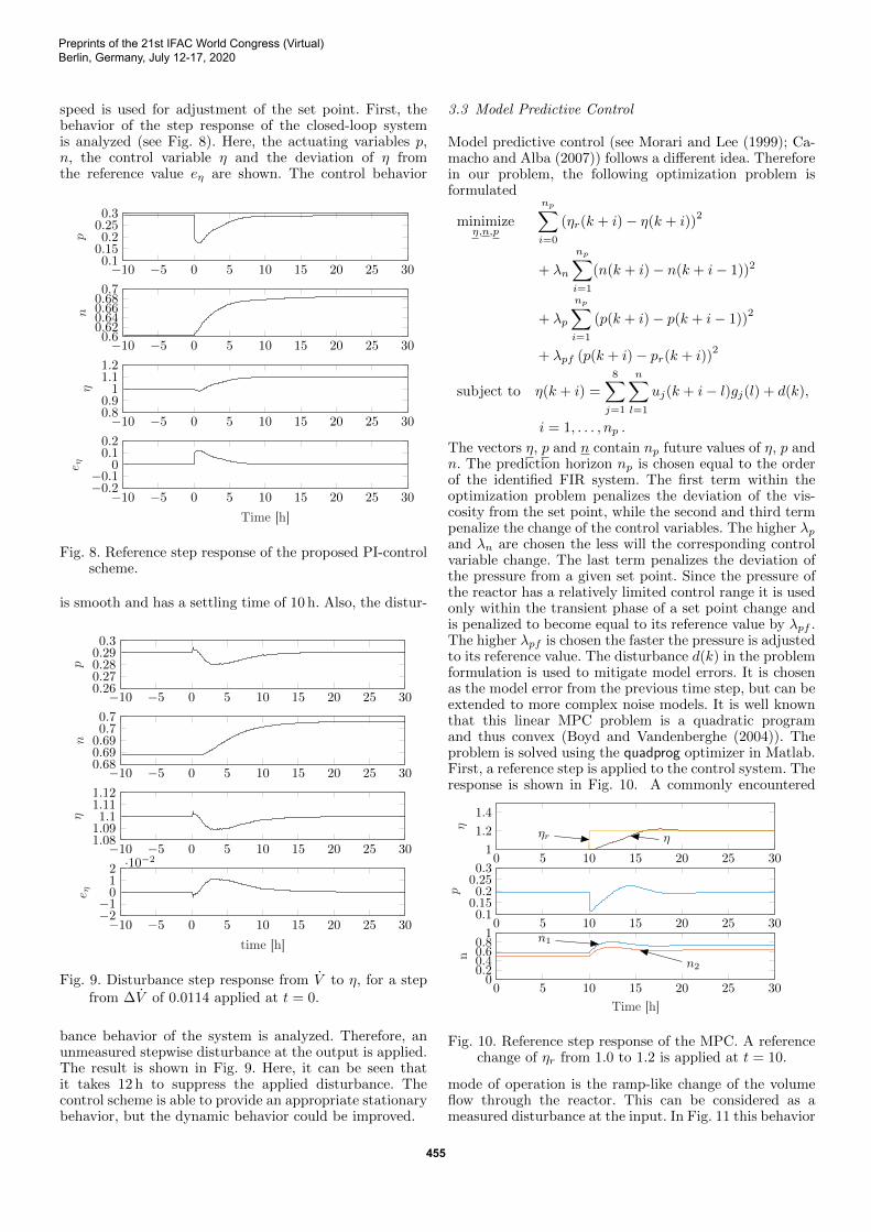
speed is used for adjustment of the set point. First, thebehavior of the step response of the closed-loop systemis analyzed (see Fig. 8). Here, the actuating variables p,n, the control variable η and the deviation of η fromthe reference value eη are shown. The control behavior

−10 −5 0 5 10 15 20 25 300.10.150.20.250.3

p

−10 −5 0 5 10 15 20 25 300.60.620.640.660.680.7

n

−10 −5 0 5 10 15 20 25 300.80.91

1.11.2

η

−10 −5 0 5 10 15 20 25 30−0.2−0.1

00.10.2

Time [h]

e η

Fig. 8. Reference step response of the proposed PI-controlscheme.

is smooth and has a settling time of 10 h. Also, the distur-

−10 −5 0 5 10 15 20 25 300.260.270.280.290.3

p

−10 −5 0 5 10 15 20 25 300.680.690.690.70.7

n

−10 −5 0 5 10 15 20 25 301.081.091.11.111.12

η

−10 −5 0 5 10 15 20 25 30−2−1012 ·10−2

time [h]

e η

Fig. 9. Disturbance step response from V to η, for a stepfrom ∆V of 0.0114 applied at t = 0.

bance behavior of the system is analyzed. Therefore, anunmeasured stepwise disturbance at the output is applied.The result is shown in Fig. 9. Here, it can be seen thatit takes 12 h to suppress the applied disturbance. Thecontrol scheme is able to provide an appropriate stationarybehavior, but the dynamic behavior could be improved.

3.3 Model Predictive Control

Model predictive control (see Morari and Lee (1999); Ca-macho and Alba (2007)) follows a different idea. Thereforein our problem, the following optimization problem isformulated

minimizeη,n,p

np∑

i=0

(ηr(k + i)− η(k + i))2

+ λn

np∑

i=1

(n(k + i)− n(k + i− 1))2

+ λp

np∑

i=1

(p(k + i)− p(k + i− 1))2

+ λpf (p(k + i)− pr(k + i))2

subject to η(k + i) =

8∑

j=1

n∑

l=1

uj(k + i− l)gj(l) + d(k),

i = 1, . . . , np .

The vectors η, p and n contain np future values of η, p andn. The prediction horizon np is chosen equal to the orderof the identified FIR system. The first term within theoptimization problem penalizes the deviation of the vis-cosity from the set point, while the second and third termpenalize the change of the control variables. The higher λpand λn are chosen the less will the corresponding controlvariable change. The last term penalizes the deviation ofthe pressure from a given set point. Since the pressure ofthe reactor has a relatively limited control range it is usedonly within the transient phase of a set point change andis penalized to become equal to its reference value by λpf .The higher λpf is chosen the faster the pressure is adjustedto its reference value. The disturbance d(k) in the problemformulation is used to mitigate model errors. It is chosenas the model error from the previous time step, but can beextended to more complex noise models. It is well knownthat this linear MPC problem is a quadratic programand thus convex (Boyd and Vandenberghe (2004)). Theproblem is solved using the quadprog optimizer in Matlab.First, a reference step is applied to the control system. Theresponse is shown in Fig. 10. A commonly encountered

0 5 10 15 20 25 301

1.2

1.4

ηr η

Time [h]

η

0 5 10 15 20 25 300.10.150.20.250.3

Time [h]

p

0 5 10 15 20 25 300

0.20.40.60.81 n1

n2

Time [h]

n

Fig. 10. Reference step response of the MPC. A referencechange of ηr from 1.0 to 1.2 is applied at t = 10.

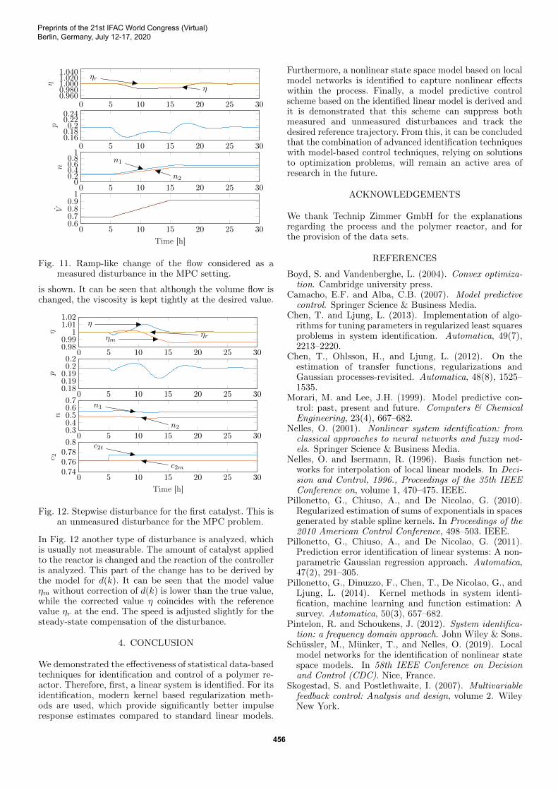
mode of operation is the ramp-like change of the volumeflow through the reactor. This can be considered as ameasured disturbance at the input. In Fig. 11 this behavior

Preprints of the 21st IFAC World Congress (Virtual)Berlin, Germany, July 12-17, 2020

455

0 5 10 15 20 25 300.9600.9801.0001.0201.040

ηr

η

η

0 5 10 15 20 25 300.160.180.2

0.220.24

p

0 5 10 15 20 25 300

0.20.40.60.81

n1

n2

n

0 5 10 15 20 25 300.60.70.80.91

Time [h]

V

Fig. 11. Ramp-like change of the flow considered as ameasured disturbance in the MPC setting.

is shown. It can be seen that although the volume flow ischanged, the viscosity is kept tightly at the desired value.

0 5 10 15 20 25 300.980.99

11.011.02

η

ηmηrη

0 5 10 15 20 25 300.180.190.190.20.2

p

0 5 10 15 20 25 300.30.40.50.60.7

n1

n2

n

0 5 10 15 20 25 300.740.760.780.8

c2m

c2t

Time [h]

c 2

Fig. 12. Stepwise disturbance for the first catalyst. This isan unmeasured disturbance for the MPC problem.

In Fig. 12 another type of disturbance is analyzed, whichis usually not measurable. The amount of catalyst appliedto the reactor is changed and the reaction of the controlleris analyzed. This part of the change has to be derived bythe model for d(k). It can be seen that the model valueηm without correction of d(k) is lower than the true value,while the corrected value η coincides with the referencevalue ηr at the end. The speed is adjusted slightly for thesteady-state compensation of the disturbance.

4. CONCLUSION

We demonstrated the effectiveness of statistical data-basedtechniques for identification and control of a polymer re-actor. Therefore, first, a linear system is identified. For itsidentification, modern kernel based regularization meth-ods are used, which provide significantly better impulseresponse estimates compared to standard linear models.

Furthermore, a nonlinear state space model based on localmodel networks is identified to capture nonlinear effectswithin the process. Finally, a model predictive controlscheme based on the identified linear model is derived andit is demonstrated that this scheme can suppress bothmeasured and unmeasured disturbances and track thedesired reference trajectory. From this, it can be concludedthat the combination of advanced identification techniqueswith model-based control techniques, relying on solutionsto optimization problems, will remain an active area ofresearch in the future.

ACKNOWLEDGEMENTS

We thank Technip Zimmer GmbH for the explanationsregarding the process and the polymer reactor, and forthe provision of the data sets.

REFERENCES

Boyd, S. and Vandenberghe, L. (2004). Convex optimiza-tion. Cambridge university press.

Camacho, E.F. and Alba, C.B. (2007). Model predictivecontrol. Springer Science & Business Media.

Chen, T. and Ljung, L. (2013). Implementation of algo-rithms for tuning parameters in regularized least squaresproblems in system identification. Automatica, 49(7),2213–2220.

Chen, T., Ohlsson, H., and Ljung, L. (2012). On theestimation of transfer functions, regularizations andGaussian processes-revisited. Automatica, 48(8), 1525–1535.

Morari, M. and Lee, J.H. (1999). Model predictive con-trol: past, present and future. Computers & ChemicalEngineering, 23(4), 667–682.

Nelles, O. (2001). Nonlinear system identification: fromclassical approaches to neural networks and fuzzy mod-els. Springer Science & Business Media.

Nelles, O. and Isermann, R. (1996). Basis function net-works for interpolation of local linear models. In Deci-sion and Control, 1996., Proceedings of the 35th IEEEConference on, volume 1, 470–475. IEEE.

Pillonetto, G., Chiuso, A., and De Nicolao, G. (2010).Regularized estimation of sums of exponentials in spacesgenerated by stable spline kernels. In Proceedings of the2010 American Control Conference, 498–503. IEEE.

Pillonetto, G., Chiuso, A., and De Nicolao, G. (2011).Prediction error identification of linear systems: A non-parametric Gaussian regression approach. Automatica,47(2), 291–305.

Pillonetto, G., Dinuzzo, F., Chen, T., De Nicolao, G., andLjung, L. (2014). Kernel methods in system identi-fication, machine learning and function estimation: Asurvey. Automatica, 50(3), 657–682.

Pintelon, R. and Schoukens, J. (2012). System identifica-tion: a frequency domain approach. John Wiley & Sons.

Schussler, M., Munker, T., and Nelles, O. (2019). Localmodel networks for the identification of nonlinear statespace models. In 58th IEEE Conference on Decisionand Control (CDC). Nice, France.

Skogestad, S. and Postlethwaite, I. (2007). Multivariablefeedback control: Analysis and design, volume 2. WileyNew York.

Preprints of the 21st IFAC World Congress (Virtual)Berlin, Germany, July 12-17, 2020

456