System Effect Factor - vpc.gr

36 ASHRAE Jou rna l ash rae .o rg Feb rua ry 2006

Syyystestem m Effectt

For a building owner concerned with operating costs, the clear-For a building owner concerned with operating costs, the clear-Fest way to document that the M&E consultant, mechanical Fest way to document that the M&E consultant, mechanical Fcontractor and testing, adjusting, balancing (TAB) contractor have

achieved the design energy consumption is to compare the energy

consumption given in the TAB equipment report with that specifi ed

in approved shop drawings.

From energy bills received for 50 new schools in Ontario, Canada (part of the 137 schools in the Dufferin-Peel Catholic dis-trict), it was evident that considerable dif-ference existed between the predicted en-

ergy consumption and actual consumption for installed equipment. Most notable was the difference in power being consumed by fan systems, prompting further investiga-tion of the data in the TAB report.

Unsurprisingly, the investigation re-Unsurprisingly, the investigation re-vealed that at the speed measured the reported fan volume and static pressure points did not intersect on the fan perfor-mance curve at the measured speed. A considerable difference existed between the measured and true static pressure in-dicated on the fan performance curve that could only be attributed to the presence of a system effect factor (SEF) after all re-corded data was checked for accuracy.

By Bernard Ratledge, By Bernard Ratledge, Life Member ASHRAELife Member ASHRAE

How it AffectsOperating Cost

Factor

About the AuthorBernard Ratledge is a building systems engineer with Dufferin-Peel Catholic District School Board in Mississauga, ON, Canada. He is a member of ASHRAE Guideline Project Committee (GPC) 1, the HVAC Commission-ing Process, and ASHRAE GPC 4, Preparation of Operating and Maintenance Documentation for Building Systems.

© 2006, American Society of Heating, Refrigerating and Air-Conditioning Engineers, Inc. (www.ashrae.org). Published in ASHRAE Journal, (Vol. 48, February 2006). For personal use only. Additional distribution in either paper or digital form is not permitted without ASHRAE’s permission.

Februa ry 2006 ASHRAE Jou rna l 37

SEF causes loss of capacity of fan volume attributed to poorly designed and installed duct fi ttings at the inlet of a single width, single inlet (SWSI) fan and axial fl ow fan, or insuffi cient clear-ance between the cabinet wall and fan inlet for a housed SWSI or double width, double inlet (DWDI) fan at the inlet and at the discharge of a both types of fans. If SEF is not considered at the design stage of a fan system, the subsequent lack of fan system performance discovered at the TAB stage may be so severe that the fan system may never operate at design volume.

Overcoming the effects of SEF often requires that the fan speed be increased, leading to higher static pressures and increased fan brake horsepower, which registers on the power demand meter, and in monthly kWh power consumption, for the life of the school building. In addition, the ambient noise level could be higher due to equipment running at higher operating speed.

Capital cost allowances for elementary and high schools are strictly controlled, but as construction costs continue to increase, architects reduce mechanical room space to accom-modate classroom space. Meanwhile, the consulting mechanical engineer is asked to fi nd innovative ways to try to fi t a gallon in a pint pot!

Consequently, fan systems are designed to be installed to preclude having the optimum ductwork confi guration at the inlet and discharge of a fan system, in accordance with the recommendations of AMCA Publication 201-02, Fans and Systems. Many design professionals remain unaware of the data available in ASHRAE Handbooks and AMCA manuals, which make it easy to identify and calculate SEF and to include it as a separate item in the fan equipment schedule.

To understand the importance of SEF, designers should be fully cognizant of how fans are tested and their performance cataloged. In all of the submitted TAB reports, a copy of the shop drawings showed the fan had the AMCA Certifi ed Ratings Seal. This seal indicates that the fan manufacturer followed the test procedures as outlined in ANSI/AMCA Standard 210-99, Laboratory Methods of Testing Fans for Aerodynamic Performance Rating (which is also ANSI/ASHRAE Standard 51-1999). This standard describes the laboratory testing procedures. AMCA Publication 203-90, Field Performance Measurement of Fan Systems, describes the fi eld performance measurements and provides critical

information as to why fi eld measurements will never plot on never plot on nevera fan performance curve.

One requirement of AMCA is that the fan manufacturer must state how that product was tested directly under the cataloged performance for a given fan model. If designers of fan systems would pay attention to these statements, problems associated with SEFs practically would be eliminated or at least minimized. The majority of fan systems installed in the schools have either a roof exhaust fan or a centrifugal fan, both SWDI and DWDI. Manufacturer’s technical literature contain typical statements associated with these types of fan as follows:

• Roof exhaust fans. Performance is based on free inlet, free outlet. Power rating (bhp) does not include drive losses. Performance ratings do not include the effects of obstructions in the airstream.

• Centrifugal fans. Performance shown is for Installation Type B. Free inlet, ducted outlet. Power rating (bhp) does not include drive losses. Performance ratings do not include the effects of obstructions in the airstream.

The fan manufacturer’s guarantee of performance is totally contingent upon the manner in which the fan was tested. None of the fans tested had obstructions, such as elbows, guards, drive sheaves or dampers, directly at the fan inlet or outlet. These types of obstructions cause additional losses that are not included in the fan manufacturer’s tests, and in many cases, are excluded in the designer’s system resistance calculations. Although most designers can easily calculate system resistance caused by fi lters, frictional resistance of ducts, and duct fi ttings such as elbows, tees, transitions, etc., which are all located some distance from the fan, they give little or no attention to obstructions close to the inlet or discharge of the fan. It is the interaction of the air with these types of obstruction that create SEFs.

Figure 1 compares how fans are tested and in many cases are installed.

Figure 1a illustrates how roof exhausters are tested. Any additional vertical straight duct on the inlet would have little, if any, effect.

Figures 1b and 1cand 1cand illustrate roof exhaust fan installations having inlet conditions that would cause SEFs.

Figure 1c illustrates the worst case because the damper is located in a turbulent airstream.


The SEF of the elbows shown in Fig-ures 1b and 1c should have single thick-ness turning vanes installed to improve airfl ow and reduce the SEF.

In Figure 1c a higher curb or extended base is desirable to increase the distance from the elbow to the damper and to the fan inlet.

Centrifugal FansFigure 2 illustrates how centrifugal

fans are tested. Many permutations of ducted inlets and outlets, multiple fan arrangements, discharge positions, and clockwise and counterclockwise rota-tions are capable of producing SEFs.

Figure 2b illustrates a poor installa-tion, with an elbow directly at the fan discharge. This type of installation can be avoided by selecting a fan with the correct rotation, and a discharge position as shown in Figure 2b. This could be im-proved further by adding a straight duct equal to 100% effective length.

Figure 3a illustrates another poor in-stallation with an abrupt discharge into a plenum. A system effect factor results if a given length of discharge duct is not present (see Figure 4 for recommended discharge ductwork).

Figures 3b and 3c illustrate installation with improper inlet conditions.

In Figure 3c the installation of a length of straight duct, equal to the fan wheel diameter between the elbow and fan inlet, would reduce the system effect factor.

The installation, as shown in Figure 3c, should be avoided if possible, because the SEF, due to inlet spin, is diffi cult to defi ne and correct.

These illustrations show some of the many installation possibilities that can create an SEF. Be aware that different

• Many housed SWSI and DWDI fans are tested as Type B, free inlet, ducted outlet. Most system designers are not aware of this rating condition and do not include any SEF for the housing.

Although it is desirable to install fan systems without SEFs, in many cases space constraints or other factors prohibit designers from providing ideal conditions.

Fan performance data and ratings are based on tests con-ducted in standardized confi gurations, which are seldom found in actual installations. In most installations, the connections between the fan and the system are likely to cause a disruptive effect (SEF) on the fl ow condition at the fan inlet and outlet. The effect of these fl ow disturbances can be signifi cantly

A B C

A B C

A B C

Figure 1a: This is typical of how roof exhausters are tested. AMCA Publication refers to this set up as “Type A: Free inlet, free outlet.” Figure 1b illustrates a poor installation with horizontal duct and an abrupt elbow at the fan inlet causing system effect. Figure 1c illustrates the same installation as Figure 1b with the addition of a damper causing even greater system effect.

Figure 2a: This is typical of how centrifugal fans are tested. AMCA refers to this set up as “Type B: free inlet, ducted outlet.” Figure 2b illustrates a poor installation with an elbow directly at the fan discharge. Figure 2c illustrates a typical installation with an elbow directly at the fan discharge. Discharge and rotation have been selected to match the fans’ fi eld conditions of Figure 2b.

Figure 3a: This illustrates a poor installation with an abrupt discharge into a plenum. Figure 3b illustrates a poor installation with an elbow directly at the fan inlet. Figure 3c illustrates a poor installation where the duct design is causing inlet spin, resulting in reduced fan performance.

types of fans are subject to different considerations based on how they were tested. Four basic installation types are shown in ANSI/AMCA Standard 210-99. The combination of all the different fan types, fan arrangements, and manufacturer’s choice of how to test provide unlimited installation possibilities are too numerous to cover in this article.

What types of fans are affected, and what condition presents the most common problems?

• Roof exhaust fans are affected by the inlet condition;• Fan types typically affected by both inlet and outlet con-

ditions are inline fans (both axial and centrifugal) and housed centrifugal fans, both SWSI and DWDI; and

Good Poor PoorGood Poor Poor

Good Poor Good

Poor Poor Poor

Rotation


Figure 4: For velocities more than 2,500 fpm, the 100% effective duct length is 2.5 duct diameters. As the blast area (area over the cutoff) decreases in proportion to the outlet area, the fl ow distortion increases, and potential system effect losses increase.

25%

50%

75%

100% Effective Duct Length

Outlet Area

Blast Area

Cutoff

Discharge Duct

greater than the pressure losses due to friction in all other system components.

Figure 5 illustrates the need to use a straight duct length on the discharge of both inline and centrifugal fans. To achieve a uniform velocity profi le, a 100% effective duct length must be used. To calculate the 100% effective duct length, use 2.5 duct diameters for 2,500 fpm (12.7 m/s) or less. Add one duct diameter for each additional 1,000 fpm (5 m/s).

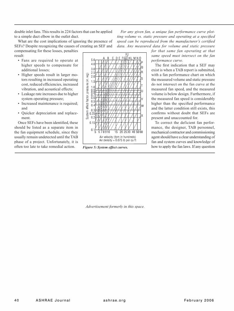
SEF cannot be measured in the fi eld. It can only be estimated. To quantify the magnitude of an SEF in an actual fan installation, AMCA has developed a method for determining an SEF. Figure 5shows a series of SEF curves. In conjunction with the location of an elbow and the effective duct length, by entering the chart at the ap-propriate inlet or outlet velocity on the abscissa, and then locating the appropriate SEF curve and reading across to the ordinate, an equivalent pressure loss is obtained for the particular confi guration and velocity. This SEF is given in inches of water gage and must be added to the estimated total system pressure losses. Where an SEF exists at the outlet and the inlet exists, the appropriate factor must be determined separately for each confi guration, and both must be added to the estimated total system pressure losses.

The development of these curves by AMCA was based on more than 100 combinations of blast area/outlet area ratio—out-let duct length—and elbow positions. For certain elbow posi-tions, an additional multiplier must be used when considering

Advertisement formerly in this space.


double inlet fans. This results in 224 factors that can be applied to a simple duct elbow in the outlet duct.

What are the cost implications of ignoring the presence of SEFs? Despite recognizing the causes of creating an SEF and compensating for these losses, penalties result:

• Fans are required to operate at higher speeds to compensate for additional losses;

• Higher speeds result in larger mo-tors resulting in increased operating cost, reduced effi ciencies, increased vibration, and acoustical effects;

• Leakage rate increases due to higher system operating pressure;

• Increased maintenance is required; and

• Quicker depreciation and replace-ment.

Once SEFs have been identifi ed, these should be listed as a separate item in the fan equipment schedule, since they usually remain undetected until the TAB phase of a project. Unfortunately, it is often too late to take remedial action.

For any given fan, a unique fan performance curve plot-ting volume vs. static pressure and operating at a specifi ed speed can be reproduced from the manufacturer’s certifi ed data. Any measured data for volume and static pressure

for that same fan operating at that same speed must intersect on the fan performance curve.

The fi rst indication that a SEF may exist is when a TAB report is submitted, with a fan performance chart on which the measured volume and static pressure do not intersect on the fan curve at the measured fan speed, and the measured volume is below design. Furthermore, if the measured fan speed is considerably higher than the specifi ed performance and the latter condition still exists, this confi rms without doubt that SEFs are present and unaccounted for.

To correct the deficient fan perfor-mance, the designer, TAB personnel, mechanical contractor and commissioning agent should have a clear understanding of fan and system curves and knowledge of how to apply the fan laws. If any question Figure 5: System effect curves.



of the equipment capability arises, the equipment manufacturer should be consulted. In most cases, the only remedial action possible is to increase fan speed. However, this option has its limitations:

• How much available horsepower remains in the installed motor?

• Does the increase in fan speed exceed the maximum allowable for the fan class rating?

• If a motor change is required, can it be accommodated on the existing fan base?

• Do the existing starter, wiring, electric overloads and heaters need to be replaced?, and

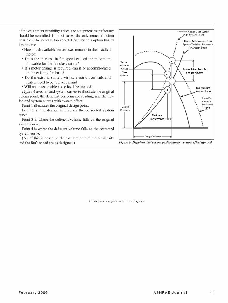
• Will an unacceptable noise level be created?Figure 6 uses fan and system curves to illustrate the original Figure 6 uses fan and system curves to illustrate the original Figure 6

design point, the defi cient performance reading, and the new fan and system curves with system effect.

Point 1 illustrates the original design point. Point 2 is the design volume on the corrected system

curve. Point 3 is where the defi cient volume falls on the original

system curve. Point 4 is where the defi cient volume falls on the corrected

system curve. (All of this is based on the assumption that the air density

and the fan’s speed are as designed.) Figure 6: Defi cient duct system performance—system effect ignored.

2

4

1

3

Defi cient Performance

Design Pressure

Design Volume

System Effect at Actual Flow

Volume

Curve B Actual Duct System With System EffectWith System Effect

Curve A Calculated Duct Curve A Calculated Duct Curve ASystem With No Allowance

for System Effect

System Effect Loss At Design Volume

Fan Pressure-Volume Curve

New Fan Curve At Increased

RPM



To further explain, let’s consider an example where the sys-tem is delivering less air than design (Point 1). The defi cient volume is Point 3 as shown on the original system curve. The original curve calculation did not include allowance for sys-tem effect. The difference between Points 3 to 4 illustrates the system effect at actual fl ow volume. The difference between Points 1 to 2 illustrates the system effect at the desired volume (design volume). Because system effect is velocity related, the difference between Points 1 and 2 is greater than the difference between Points 3 and 4.

Points 2 and 4 fall on a new system curve. For the existing fan to produce the design volume (Point 2) on the new system curve, the fan speed must be increased.

To illustrate the above, the following presents two examples of TAB data reported for actual fan installations.

Example 1This data is for a DWDI inlet fan, backward-inclined airfoil

wheel, housed in an enclosure as part of a packaged air-handling unit supplying air to classrooms. Fan volume is established by taking three branch duct traverses and outlets on a branch duct not traversed.

Design System RequirementsDesign System RequirementsVolume: 18,100 cfm (8542 L/s)Fan static pressure: 4.28 in. w.g. (1.065 kPa)Fan speed: 1,443 rpm (24.05 rps)Fan hp: 17.69 (13.2 kW)

Test DataVolume via duct traverses: 17,961 cfm (8477 L/s)Volume via outlets: 17,117 cfm (8078 L/s)Fan static pressure: 3.08 in. w.g. (766 Pa)Fan speed: 1,432 rpm (23.87 rps) Fan hp: No data givenSince no fan performance chart was submitted, the data could

be interpreted in three different ways:1. Data as reported is correct;2. Static pressure is correct, but fan volume is incorrect; and3. Volume is correct, but static pressure is incorrect.The measurements were checked and the only reliable mea-

surement was fan speed.Although the difference between the volumes obtained at

the outlets and measured at the duct traverses was small, the difference between the design requirement and that obtained at the outlets was enough to warrant an increase in fan speed to achieve the design requirement.

Let us now examine each interpretation.

1. Data as Reported is Correct.Assuming the original test data is correct, calculations to

increase the fan speed to achieve the design volume are based on this data. To compound the problem, a 5% leakage occurred in the ductwork. How can we compensate for this?

Proceed as follows:

Based on the reported data of 17,961 cfm (8477 L/s) at 3.08 in. w.g. (766 Pa) at 1,432 rpm, a system curve was produced and found to intersect the fan performance curve at 19,820 cfm (9353 L/s) at 3.75 in. w.g. (934 Pa) and 17.51 bhp (13 kW). Since the duct traverse measurements were taken some distance from the discharge of the fan, the difference between the calculated fan volume and measured volume could be at-tributed to leakage or inaccurate traverse readings.

Point 1 in Figure 6 is represented by the value of 19,820 Figure 6 is represented by the value of 19,820 Figure 6cfm (9353 L/s).


To achieve the design volume of 18,100 cfm (8542 L/s), a new system curve must be produced. The outlet volume of 17,117 cfm (8078 L/s) is plotted on the original system curve, point of intersection: 17,117 cfm at 2.797 in. w.g. (8078 L/s at 693.52 Pa) Point 3 on Figure 6 and a line projected vertically from this point to cut the actual fan curve at 17,117 cfm at 4.41 in. w.g. (8078 L/s at 1097.3 Pa) to represent Point 4 on Figure 6.

A new system curve then is calculated to produce a new fan operating point of performance as follows:

I-P

cfm1 rpm1 17,117 1,432 = = =

cfm2 rpm2 18,100 rpm2

18,100 × 1,432 rpm2 = = 1,514 17,117 rpm 17,117 rpm2 17,1172

in. w.g.1 rpm12

4.41 1,432 2

= rpm rpm = = 4.41 1,432 4.41 1,432 in. w.g.2 rpm rpm 2 in. w.g. in. w.g.

2 1,514 1,514 4.41 in. w.g. 4.41 in. w.g. 4.41

2 = = 4.93 in. w.g.

1,4322

1,514

SI

L/s1 rps1 8078 23.87 = = =

L/s2 rps2 8542 rps2

8542 × 23.87 rps2 = = 25.23

8078

Pa1 rps12 1097.38 23.87

2

= rps rps = = 1097.38 23.87 1097.38 23.87 Pa2 rps rps 2 Pa2 25.23 25.23

1097.38 Pa2 = = 1226.78 Pa

23.87 2

25.23

The revised fan performance curve for the system to operate at design volume shows the following:

18,100 cfm at 4.93 in. w.g. (8542 st 1.227 kPa) at 1,514 rpm


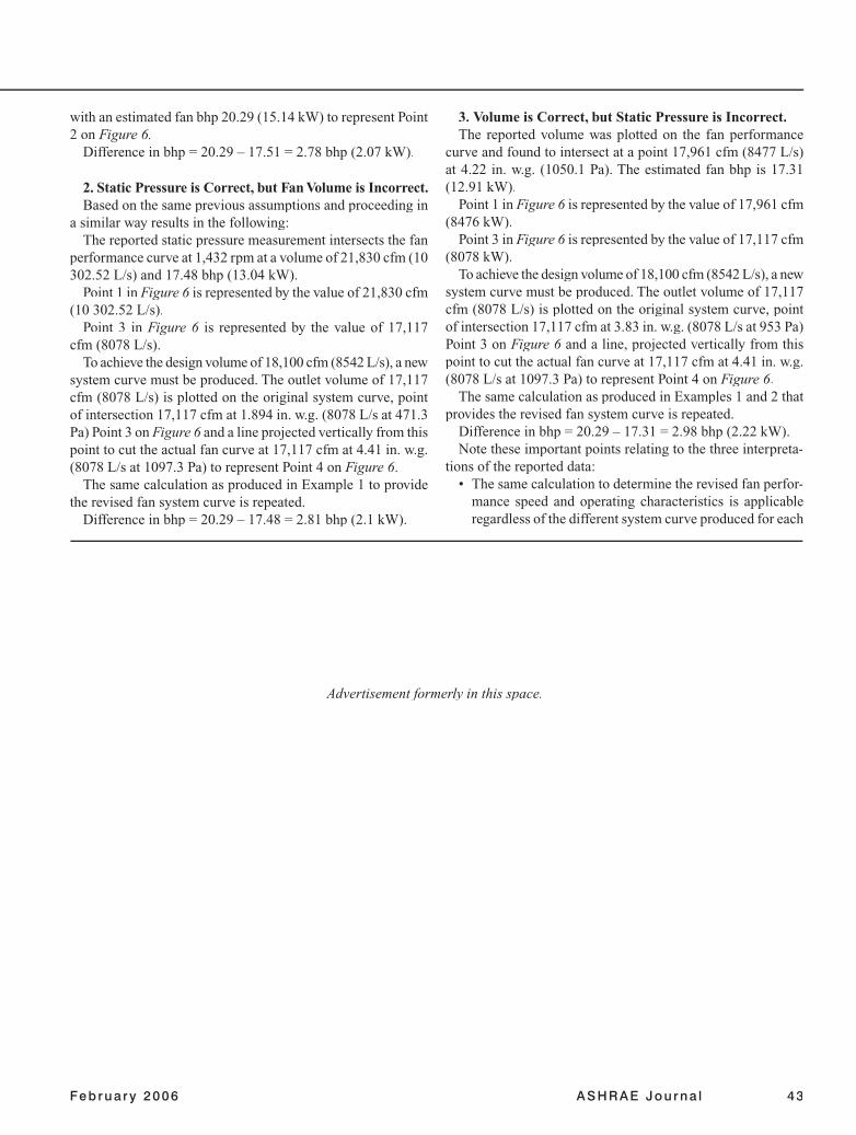
with an estimated fan bhp 20.29 (15.14 kW) to represent Point 2 on Figure 6.

Difference in bhp = 20.29 – 17.51 = 2.78 bhp (2.07 kW).

2. Static Pressure is Correct, but Fan Volume is Incorrect.Based on the same previous assumptions and proceeding in

a similar way results in the following:The reported static pressure measurement intersects the fan

performance curve at 1,432 rpm at a volume of 21,830 cfm (10 302.52 L/s) and 17.48 bhp (13.04 kW).

Point 1 in Figure 6 is represented by the value of 21,830 cfm Figure 6 is represented by the value of 21,830 cfm Figure 6(10 302.52 L/s).


To achieve the design volume of 18,100 cfm (8542 L/s), a new system curve must be produced. The outlet volume of 17,117 cfm (8078 L/s) is plotted on the original system curve, point of intersection 17,117 cfm at 1.894 in. w.g. (8078 L/s at 471.3 Pa) Point 3 on Figure 6 and a line projected vertically from this Figure 6 and a line projected vertically from this Figure 6point to cut the actual fan curve at 17,117 cfm at 4.41 in. w.g. (8078 L/s at 1097.3 Pa) to represent Point 4 on Figure 6.

The same calculation as produced in Example 1 to provide the revised fan system curve is repeated.

Difference in bhp = 20.29 – 17.48 = 2.81 bhp (2.1 kW).

3. Volume is Correct, but Static Pressure is Incorrect.The reported volume was plotted on the fan performance

curve and found to intersect at a point 17,961 cfm (8477 L/s) at 4.22 in. w.g. (1050.1 Pa). The estimated fan bhp is 17.31 (12.91 kW).

Point 1 in Figure 6 is represented by the value of 17,961 cfm Figure 6 is represented by the value of 17,961 cfm Figure 6(8476 kW).

Point 3 in Figure 6 is represented by the value of 17,117 cfm Figure 6 is represented by the value of 17,117 cfm Figure 6(8078 kW).

To achieve the design volume of 18,100 cfm (8542 L/s), a new system curve must be produced. The outlet volume of 17,117 cfm (8078 L/s) is plotted on the original system curve, point of intersection 17,117 cfm at 3.83 in. w.g. (8078 L/s at 953 Pa) Point 3 on Figure 6 and a line, projected vertically from this Figure 6 and a line, projected vertically from this Figure 6point to cut the actual fan curve at 17,117 cfm at 4.41 in. w.g. (8078 L/s at 1097.3 Pa) to represent Point 4 on Figure 6.

The same calculation as produced in Examples 1 and 2 that provides the revised fan system curve is repeated.

Difference in bhp = 20.29 – 17.31 = 2.98 bhp (2.22 kW).Note these important points relating to the three interpreta-

tions of the reported data:• The same calculation to determine the revised fan perfor-

mance speed and operating characteristics is applicable regardless of the different system curve produced for each



assumed condition. Only one point on the original fan curve (Point 4) exists for determining the revised actual system curve with system effect;

• When attempting to establish the existing fan bhp, it is imperative to include fan bhp calculations with each fan test to compare between existing and future fan power consumption estimates; and

• If the measured data is to be believed, it is imperative that it is interpreted and reported correctly to maintain the integrity of the TAB report. The TAB report may be the only document an owner has to judge whether the designer, contractor, TAB contractor and commissioning agent have fulfi lled their contract obligations.

After further examination of the fan housing and discharge duct, the presence of an SEF at the inlet and outlet was con-fi rmed. The inlet SEF was due to insuffi cient clearance be-tween the fan inlet and housing wall and SEF at discharge due to insuffi cient length of straight duct between fan discharge and elbow. The actual, correct operating point was quoted in Example 3.

The increase in hp, i.e., 20.29 – 17.31 = 2.98 hp (15.13 – 12.91 = 2.23 kW) is the extra horsepower that will register on the utility meter for the life of the building. In addition, the original motor was 20 hp (1492 kW) and needs to be increased

to 25 hp (18.65 kW). Based on the fan operating 245 days × 8 hrs/day × 12.91 = 25,303.6 kWh × $0.06/kWh = $1,518.21 + 12.91 × $10/kW demand × 12 = $3,067.41/yr base electric cost. Revised operating cost with new motor = 245 days × 8 hrs/day × 15.13 = 29,654.8 kWh × $0.06/kWh = $1,779.28 + 15.13 × $10/kW demand × 12 = $3,594.88/yr or $527.47/yr increase. A life-cycle analysis based on a school useful life of 25 years, annual energy cost escalation 5%, shows an estimated total additional operating cost of $30,212.

Example 2The reported data is for a centrifugal, backward-inclined

airfoil plenum fan installed in a heat recovery unit providing ventilation air to all classrooms and makeup for all other exhaust systems. This fan is the exhaust air fan in the unit. Therefore, it is imperative that the volume from each class-room is as designed to maintain a CO2 level <800 ppm in the occupied space.

Design System RequirementsDesign System RequirementsVolume: 13,220 cfm (6239 L/s)Fan Static Pressure: 2.6 in. w.g. (647 Pa)Fan Speed: 1,396 rpm (23.26 rps)Fan hp: 8.53 (6.36 kW)



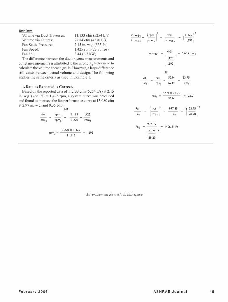
Test DataVolume via Duct Traverses: 11,133 cfm (5254 L/s)Volume via Outlets: 9,684 cfm (4570 L/s)Fan Static Pressure: 2.15 in. w.g. (535 Pa)Fan Speed: 1,425 rpm (23.75 rps) Fan hp: 8.44 (6.3 kW)The difference between the duct traverse measurements and

outlet measurements is attributed to the wrong Ak factor used to calculate the volume at each grille. However, a large difference still exists between actual volume and design. The following applies the same criteria as used in Example 1.

1. Data as Reported is Correct.Based on the reported data of 11,133 cfm (5254 L/s) at 2.15

in. w.g. (766 Pa) at 1,425 rpm, a system curve was produced and found to intersect the fan performance curve at 13,080 cfm at 2.97 in. w.g, and 9.35 bhp.

I-P

cfm1 rpm1 11,113 1,425 = = =

cfm2 rpm2 13,220 rpm2

13,220 × 1,425 rpm2 = = 1,692 11,113 rpm 11,113 rpm2 11,1132

in. w.g.1 rpm12

4.01 1,425 2

= rpm rpm = = 4.01 1,425 4.01 1,425 in. w.g.2 rpm rpm 2 in. w.g. in. w.g.

2 1,692 1,692 4.01 in. w.g. 4.01 in. w.g. 4.01

2 = = 5.65 in. w.g.

1,4252

1,692

SI

L/s1 rps1 5254 23.75 = = =

L/s2 rps2 6239 rps2

6239 × 23.75 rps2 = = 28.2

5254

Pa1 rps12 997.85 23.75

2

= rps rps = = 997.85 23.75 997.85 23.75 Pa2 rps rps 2 Pa2 28.20 28.20

997.85 Pa2 = = 1406.81 Pa

23.75 2

28.20





To achieve the design volume of 13,220 cfm (6239 L/s), a new system curve must be produced. The measured volume of 11,133 cfm (5254 L/s) is plotted on the original system curve, point of intersection: 11,133 cfm at 1.297 in. w.g. (5254 L/s at 322.74 Pa) Point 3 on Figure 6 and a line projected verti-Figure 6 and a line projected verti-Figure 6cally from this point to cut the actual fan curve at 11,133 cfm at 4.01 in. w.g. (5254 L/s at 997.85 Pa) to represent Point 4 on Figure 6.

A new system curve is then calculated to produce a new fan operating point of performance as follows:

The revised fan performance curve for the system to operate at design volume shows the following: 13,220 cfm at 5.65 in. w.g. at 1,692 rpm with an estimated fan bhp 16.83 (12.55 kW) to represent Point 2 on Figure 6.

Similarly, by applying the same criteria as Items 2 and 3 in Example 1, the difference between the future and existing power consumption can be established. The actual static pres-sure was established at 4.01 in. w.g. after all measurements were checked. Fan power was at 10.06 bhp.

The increase in fan bhp = 16.83 – 10.06 = 6.77 (12.55 kW – 7.5 kW = (5.05 kW).

Using the same operating parameters as Example 1:Based on the fan operating 245 days × 8 hrs/day × 7.5 =

14,700 kWh × $0.06/ kWh = $882 + 7.5 × $10/kW demand × 12 = $1,782/yr base electric cost. Revised operating cost with new motor = 245 days × 8 hrs/day × 12.55 = 24,598 kWh × $0.06/ kWh = $1,475.88 + 12.55 × $10/kW demand × 12 = $2,981.88/yr or $1,199.88/yr increase. A life-cycle analysis based on a school useful life of 25 years, annual energy cost escalation 5%, shows an estimated total additional operating cost of $86,489.

Since April 1997, the approximate total number of fans systems installed and tested is 1,500. However, out of all the TAB reports, not a single fan performance curve was included with each fan system submitted. The owner’s staff produced fan performance curves for every fan system that showed that the fan operating point, as reported, did not intersect at the measured volume, static pressure and fan speed. A sub-sequent examination of each fan installation showed an SEF was responsible for defi cient fan volume.

A detailed analysis of each TAB report revealed that there was a 15% to 25% increase in the difference between the predicted and actual fan hp, which were all attributable to the presence of SEFs in each fan system.

Every fan system test should be accompanied by a copy of the fan performance curve at the measured speed.

Three variables are associated with any fi xed point on a fan performance curve at any given speed: fan volume, static pressure, and fan bhp.

The volume and any of the other variables must intersect on must intersect on must

the fan performance curve at the given speed. If they do not intersect, after checking each respective value for accuracy, then there is an SEF that must be accounted for to establish the true operating point. The SEF may exist on the suction, discharge, or both sides of the fan.

How to Avoid This Increased Operating Cost?• By not trying to save dollars per square foot by reducing

the size of the mechanical room. The increased operat-ing cost of the poor installation is likely to be far greater than the cost of providing the space necessary to ensure a good ductwork installation.

• By designing the system to ensure that it operates as in-tended and to ensure that the mechanical contractor, TAB contractor, and commissioning agent fully understand the ramifi cations of the presence of an SEF.

• By making alterations to the ductwork, if possible, since the penalties infl icted by SEFs are present for the life of the building.

• By ensuring that if SEFs cannot be avoided, they are ac-counted for and shown as a separate item in the contract documents.

• By showing this as a separate item in the contract docu-ments and indicating to the mechanical contractor, TAB contractor, and commissioning agent, that the measured values during fan performance testing do not show the not show the nottrue fan total static pressure and by ensuring that the SEF is calculated and added to the measured value.

• By ensuring that the TAB specifi cation clearly indicates how the system is to be tested (AMCA Publication 203-90), and that procedure is used for calculating the SEF (AMCA Publication 201-02) and is included in the TAB report.

• By stipulating in the equipment and TAB specifi cations that a fan performance chart be submitted for every fan tested showing the system operating point. The equipment manufacturer must provide the fan performance curve as part of the submittal. The TAB fi rm is to be given this chart and an approved submittal for the fan.

SummaryThe importance of recognizing the penalties that will be in-

curred due to SEFs cannot be overstated. They will impact the energy bill for the life of the schools. Remedial work will be costly and delay the operation of the school’s HVAC systems. The examples illustrate the penalty each fan system could incur. No reason exists to believe the remaining systems are any different. However, the overall penalty for all 137 schools in the Dufferin-Peel Catholic District during a 25-year period could exceed $15 million to $20 million.

Paying attention to detail at the design stage and ensuring that fans are installed without incurring an SEF provides the only solution to avoiding these additional installation and operating costs.

Documents

System Effect Factor - vpc.gr