TRANSPORTATION RESEARCH RECORD 1274 63

System Dynamics Modeling of Development Induced by Transportation Investment

DONALD R. DREW

A modeling paradigm for analyiing transportation-development interactions is de cribed. The new approach is ba ed on i olating underlying cau e of development deficiencies in a ystematic way identifying policie and infrastructure inve tment to deal with the cause , and then as essing the impacts of alternatives against specified goals. The system dymtmics methodology uses three a lterna tive form of the model: verbal (narrative descrip­tion) , visual (causal diagram) , and mathematical (set of equation derived from rhe cau al diagram) . The methodology is illustrated using three examples: (a) modeling urban sy. terns, (b) modeling regional and national economics, and (c) evaluating user and nonuser benefits .

Reducing the tru cost of transport increa es the total amount of good and ervices available, ultimately increa ing the total real income of any society. Tools for estimating the effects of different transportation improvements within these contexts are only now being developed. These tools tend to fall into two classes: (a) models of national and regional economies with a component being the transportation system; and (b) traditional models of various aspects of the development pro­cess such as land use models, population models, location models, economic base models and input-output models that are linked either explicitly or implicitly to transportation.

NEED FOR MODELING PARADIGM

Although there are well-established professional activities associated with transportation problems (transportation plan­ning, transportation operations, and transportation econom­ics) and well-established profe sional activities associated with development problems (development planning, development economics, and development administration), the two classes of activities are usually linked subjectively. Moreover, the actual decision-making processes in each proceeds with nearly total isolation from ongoing planning activities. A new approach is needed for isolating underlying causes of development defi­ciencies in a systematic way, identifying policies and infra­structure investments to deal with the causes, and then assessing the impacts of alternatives against specified goals .

The whole process starts with a basic restatement of values and goals. Values are those irreducible qualities on which individual and group preferences are based. The groups are defined as the users of transportation, the providers of trans-

Department of Civil ngineering, Virginia Polytechnic Institute and State University, Blacksburg, Va . 24061.

portation, and the society. Goals are desirable end-states toward which planning might be expected to lead. A problem exists when a goal is not being achieved. There may be two possible reasons for this failure: (a) the goal is unachievable and (b) the problem re ults from conflicting goals. There is oot much that can be done in the fir t ca e except to lower aspiratio.ns . In the second case, the problem may be described as an issue­a matter that is in dispute between two or more of the three groups involved (1).

rn all there are three ways in which cau ality from a policy­controlled variable acts on a goal or uncontrolled variable: (a) the sign of the interaction (po ·itive or negative) (b) the trength of the interaction ( ·trong or weak) and (c) the time

lag of the influence. Moreover because policy variable may act indirectly on several different goal · through causal sequences of intermediate variables, cross-impact analysis is best accom­plished using a digital computer. The ultimate result i one o[ creating cenarios- determining future impacts of contem­plated policie by setting logical sequences of event in ·tep-by-step relationships (2),

A ystem perspective of transportation development anal­ysi. requires consideration of software (policies) a well as hardware (technologies) , time as well a pace, and stra­tegic as well a tactical method . The principal requirement for viable strategic approache · to olving transportation­development problem i that the approaches be system-wide, causally ba ed , and policy-oriented, and permit the ·pecifi­cntion of alternative transportation-development concepts in sufficient detail to allow their implications and impacts to be examined.

SYSTEM DYNAMICS APPROACH

Transportation systems-particularly highways, ports, and airports-are essential to the efficient functioning of national economies throughout the world, but experts say that these systems will be increasingly burdened by ever-growing demand, limited supply, and increased congestion. Although trans­portation systems are particularly vital to national and regional economic productivity, no organized or well-developed body of knowledge exists regarding the effects of transportation infrastructure on development. Indeed, engineers and plan­ners dealing with transportation problems rarely work closely with their counterparts in economic development.

The transportation-development relationship is essentially a two-way interactive process with results of the interaction

64

depending on the type of economy involved and on the level of development at which transport improvements are effected. Al a given level of developmem an area requires a certain level of transportation to maximize its potential. Thus, an optimum tran portation capacity correspond to any devel­opment level. Existence of unsati fied demand for transpor­tation may, over time, have seriou adverse effect on the economy: conversely. th re. ults of overcapitalization may be unpleasant if too much money is pent on tran portation in anticipation of demand that never materialize (3 4).

A model of this proces · can be complex and can consist of hundreds of variables. Because of the necessary feedbllcks, determining the optimal transport system consi tent with a specific spatial structure of an area is, to say the least, elusive (5).

Research is needed to develop a methodology for con­structing regional transportation-development models. Such a methodology wou ld start with verbal descriptions of per­ception of the proces . From these verbal descriptions key variables and their interactions would b identified and dis­played graphically in the form of cau al diagrams. Using th causal diagrams mathematical model, would be developed. Verbal de cription is important in explaining the reasoning leading to a proposed policy and !'he consequence f Lhat policy. Graphical display provides a gestalt for synth izing the contribution of expert and specialists. Mathematical model. provide an in 'lrumen1ali1y that can be ubject to manipulation and ensitivity analy ·is . By examining the en­sitivitie of hypothesized relationship. prioritie for data collection for model calibration can be established (6).

Although experts may understand portions of the transporlation-economic development process, to synthesize these portions in a consistent manner without a formal t ch­nique is impo ible. The tran portation-development process is composed of large numb r f variables :.-panning many disciplines. These variables are causally related and clo e on them elve to form higher-order feedback loop'. Inputs are stochastic, relationships are nonlinear, and delays and noise are present in the information channels. All of these char­acteristics preclude predicting ' ystems behavior by partition­i11g the problem along disciplinary lines and then assembling the component olutions (7).

THE MODELING PROCESS

Policy makers, to guide national development effectively, must bring together a variety of mental model , translate them into a common language, and then determine simultaneously all their important implications. Therefore formal models with os umption stated e.,plicitly are required. Formal models are best expres ·ed in math matical equations for three rea on : (a) mathematics is precise and interdi ·ciplinary. (b) equati n can be manipulated in re ponsc Lo changing inpu1s and (c the mathematical notation permit processing by computer.

For system dynamics meth dology , three alternative form" of the model of a system are used: verbal, visual, and math­ematical (8). The verbal description is a mental model of the y tern expressed in words . Visual descriptions arc diagram­

matic and show cause-and-eff ct relati nships between many variables in a simple, concise manner. The vi ual model, or causal diagram, is then translated into a mathematical model

TRANSPORTATION RESEARCH RECORD 1274

of system equations. All forms are equivalelll, with any one form merely serving as an aid to understanding for someone who does not comprehend the other forms. However, the verbal descrip1ioa doe not lend itself t f rmal analysis and the visual cau al diagram can only be analyzed qualitatively. Mathematical model · are by far the most precise and are the only representations of the system that permit quantitative analysis and the evaluation of nlternutivc solutions to a problem.

Modeling procedure is sequential and iterative and starts with the verbal d cription of the major elements nece ary to represent relevant aspects of the . ystem_ Next is the pos­tulali n of the model' truclure and conceptualization of causal relationships between model parameters in the form of a causal diagram. From the causal diagram, ysl m equations may be written. In order to complete the mathematical model, the model 's param tcrs mus! be estimated. his tep includes placing numerical values on constants and the quantifi ation of causal as umptions. Th accuracy of the model can be evaluated through simulation. At each step, the model is exposed to criticism, revision, reexposure, etc ., in an iterative process that continue as long as it proves us fuJ (9).

The p.ropo. ed methodology use all f the relevant param­eter cla ·e in system dynamic - level variable , rate varia­bles, auxiliary variables, supplementary variables, and con­stants. However, the methodology is different because the geometric shapes-rectangles, valves, circles, etc.-used in system dynamic diagram. are unneces ary . F r example. a level variable is always at the head and a rate variable i always at the tail of a ·olid arrow. igns on the olid arrow indicate if the rate is added to or subtracted from the level of the state variable. Whereas solid arrows denote physical flows , dashed arrows in the causal diagram define information flows from level variables to rates, or action, varia le . Any intermediate variable on the path from a level variable, or from an exog­enou input, to a rate variable i, called an auxiliary variable. Signs on da hed arrows have the following inrerprctation: a plu sign ( +) means that an increase in the parameter at the tail of !'he arrow will cau e an increa e in rhe variable at the head of the arrow; a minus sign ( - ) means that an increase in the parameter at the tail of the arrow will cause a decrease in the parameter at the head of the arrow. Exogenous inputs are easily identified on a causal diagram becaus they have no arrows leading to them, but have one or more dashed arrows emanating from them. Supplementary variables, in contra t, do not form part of the y tem itself but mere ly indicate its performance and, therefore , are ah ays identified hy heing at the head of a dashed arrow nnd having no arrows emanating from them . In summarizing the causal diagram­ming convention: (a) arrows describe the direction of cau ·ality between pnir of variables, (b) li 11i::s (suliu ur dashed) denote (phy ical or inf rmation) now , and (c) signs indicate the nature (direct or inverse) of the relationship between dependent-independent variable pairs.

The methodology use the DYNAMO computer language a ociated with system dynamics. In differenc equation terminology any level variable L is expres ed as a function of rate variables 1~ 1 and the previous value of tbe level.

n

L;(t + dt) = L;(t) + (dt) 2:: Rj(t) j=l

1 = 1, ... , m (l)

Drew

with R1 values assumed constant over the time interval from t to t + dt. The rate variables are in the form

(2)

where Ek are the set of exogenous inputs that affect variables R; directly, and A,; and Ak; are the impacts of auxiliary var­iables in the causal streams from the ith variable and kth exogenous input, respectively. Because exogenous inputs are known time functions or constants, if initial values of the level variables are known, all other variables can be computed from them for that time. Then, new values of the level variables for the next point in time can be found from Equation 1. DYNAMO uses a postscript notation for subscripts in which .K stands for the present time t, .J stands for past time t - dt, and .L stands for future time t + dt. As in all computer programming, upper-case letters are used. DT (dt) is called the solution interval, the time between successive computa­tions in the simulation. Because rate variables are assumed to be constant over DT, the double postscript is used, .JK for rates on the right side of an equation and .KL for rates on the left side.

MODELING URBAN SYSTEMS

Impacts of transportation on national development are usually focused on urban areas. Transportation is the bloodstream of the urban community because spatial interdependence is the rationale of the urban area. A given transportation system both influences the location of activities within the city and is itself influenced by the location of these activities, because each location pattern constitutes a set of trip demands that is responded to by investment and operating decisions within the transportation system. Unfortunately, despite this stra­tegic importance, the system may diverge from efficient resource use on a number of grounds-economies of scale, mixed public and private sector decision making, and lack of coor­dinated decision making for the affected metropolitan area and across different transportation modes. Before modeling the impact of transportation on regional or urban develop­ment, a model needs to be developed for the region or the urban area, whichever applies.

Urban systems can be arbitrarily divided into two cate­gories: (a) those that are related to the urban socioeconomic structure such as social, industrial, and residential systems; and (b) those that serve the urban community (the urban technological systems) such as water supply, energy, trans­portation, and the environment. Basic knowledge of how the urban systems are formed and interact with each other pro­vides a basis for a better learning process and, thus, a better decision-making process. Because of interrelationships between urban systems, a sound solution to an urban problem can hardly be attained without knowing the possible effects on other systems. Lack of understanding of this causality in fore­casting usually leads to treatment of symptoms rather than causes.

In a system as complex as a city, intuition has proven most unreliable in forecasting the probable consequences of well­meaning policies, simply because the human mind is incapable of dealing with a system containing so many variables. No wonder that urban policies, laws, and decisions have produced results different from those intended, ranging from partial

65

success to tragic failure. Predicting with confidence the long­term consequences of costly programs has been impossible. One of the main causes leading to the failure of many urban development programs is the inability to experiment with the designed policies. Usually, a policy is implemented on the basis of some informally estimated consequences and a few decades later the policy turns out wrong. Therefore, in a decision-making process, facts must be included, but facts about future events cannot be obtained.

With present technology, one means of studying future events is through computer simulation, which is not only economical, but also is a powerful conceptual device that can increase the role of reason at the expense of rhetoric in determining effec­tive policies. Unlike intuition and common sense of informal mental models, computer simulation is comprehensive, unam­biguous , flexible, and subject to logical manipulation and test­ing. Flexibility of a system dynamics model is its least appre­ciated virtue. If there is disagreement about some aspect of causal structure or the strength of effects between variables of a problem, in a short time the model can be rerun and observations made of its behavior under each set of assump­tions. Often, the argument is trifling because the phenomenon of interest may be unchanged by the factor in disagreement.

To illustrate the system dynamics approach to modeling transportation-development interactions, three examples will be presented. The first, METRO, is a model of a metropolitan area consisting of a central city and its suburbs. The model comprises seven sectors (city population, industry, housing, employment, land, suburban carrying capacities, and trans­portation) that will be described in the traditional system dynamics format: verbally, by causal diagrams, and by DYNAMO equations.

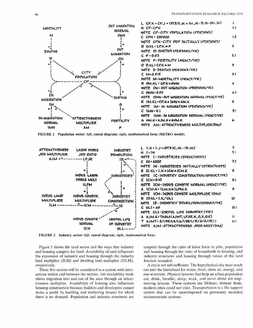
First, the population sector of the central city is displayed in causal diagram form and in equation form (Figure 1). The level variable CP, for city population, is controlled by two types of rates: natural increase (births and deaths) and migra­tion in and out. Each of these four rates depends on the population and constant fractional rates of increase. How­ever, in-migration is also assumed to be influenced by an attractiveness multiplier .

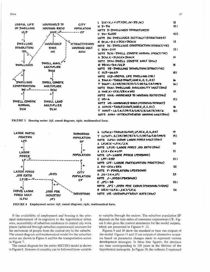
Next, Figure 2 shows the industry sector. Although many ways of measuring economic activity are available, industry is chosen as the level variable for this sector. Industries create more industries through industry construction. Amounts of additional economic activity are proportional to the present rate of economic activity. So, at every point in time, industry construction equals the number of industrial structures mul­tiplied by industry construction normal with the word "nor­mal" denoting the conditions under which construction occurs. Conditions within the urban area such as labor availability and land availability that encourage or discourage construc­tion (above or below the normal fraction, respectively) are handled by an industry construction multiplier.

The housing sector, which is shown graphically and math­ematically in Figure 3, is handled in a manner similar to the industry sector, except that the basic structural unit is the dwelling instead of the industry.

The employment sector relates the demographic (popula­tion) and economic (industry) sectors. Population determines the size of the labor force, that is, the demand for jobs. Industry creates jobs-the supply side of the interaction (see Figure 4).

66

MOITTALITY

M I I I +• . t

l)f:ATil5

OUT MIGR:ATIO>J NOll!MAL

OMN I I '+ ' OUT

TRANSPORTATION RESEARCH RECORD 12 74

l Cf'.K • CP.J + <PTJ(D.JK + IM.Jfc:-lU"·OM.JK) N Cf'•Cf'M NOTE CP-CITY POPULATIOM (Pf'llSONS) C Cf'N • 190000 NOTf CF'N-CITY POP lN1TIALLY(Pf~SOflJ5) R: l).KL • CP. K « F wore 13· 01~5 <restsoM51Yll> C F•O.O~ NOTE F- FfSfTILITY ( R{ACT /Y'~) R 1>.KL•CP.K•M NOTf J>· PCATH~ (l'ell,OMS/YK) C M•0.015 NOTf M-MOstrALITY lFt{ACT/YJC) R: OM.l<L• Cr!l<•OMN HOT'f OM- OUT MIGltATION (f"eR'SONS/YI.:) C OMN•O.O'J HOTC OMN •OUT MIGltATIDN NO!tMAL I FS:ACT/Ylt) R: lM.KL•CP.1<• IMN«AM.K NOTe IM· IN M~•TION (f'tllSON5~) C JMN•O.l Nort IMN • IN Ml~IV.TION NORMAL (FIUCTIYR) A AM.K•AJM.K4AMM.I< NOTe AM· ATTltACTl~N~~ MULTIPl..ltR:CPIM)

u

l.Z

z. t

'·'

4.1

'·'

FIGURE 1 Population sector: left, causal diagram; right, mathematical form (METRO model).

ATTflACTIV!N~5' LADOlt FOlt'Ct L t.K • l.J HPTX IC.JI< -11>.JK) .., IND~TR:Y N I• JN ':J.1

JOI) MULTIPLlest JOI) R'ATIO J>eMOLITION AJM •=-------- LFJK

'is::~-, NOTf l- lMt)U5Tstlf~ lSTll!UCTURf~)

I C IN•~ "f.Z I

HOTf IN· INVU5TRIC:~ INITIALLYl5TIWCl\Jltf5) I

+l - \ fl JC.l(L• l.l<«lC.N«ICM.K 6

' INPU! LADOR JNl>USntte~' NOTC IC· INl>USTilY CON$TRUCllOW (5T~UCT ~) ~ce MULT.

,,,, C ICN•0.10 e.1 ,,

ILFM I I NOTe lC.N-H@U!) CON5T~ NO'™AL(~CT/Y!C)

I \ ' j+ I A ICM.K• ILM.1<.,.lLFM.K 9 +~ ~ .,

wore 1CM- IM1'U5 CO~TIZ MlJL 11PLI~ (l>IM) JNl)US. u.NP INOU! cowsm. \Nl) :STft'f I I R l1M(L• l.l(/ULI to

MULTIPLleR MVLTIPLletC CONSTKUCTION : NOT? 11' • I H'J)WMY' 1>CMOLl110IJ (STltUCf /Vlt)

ILM --------s-1cM---------t ... 1c I / I C UU•.CO 10.\

...... "'+ I NOTt lJLl-UStfUL LIFC lHJU5T~(VK) ,,,, I A AJM.l<•TAOl.t(AJMT. LFJR.K,0,2.0.2) II ...... I

INP\a CON5T".' °'eFULUFE T AJ MT• 1/1. ff /l.f /1."/I. n/1/..,./.5/. 2/. /'5/. I II.I NORMAL

I OFINPU,TRY I NOTC AJM·ATTlfACTivttJ~5 J005 MULTCJll'M)

JCN ULl----"' I

FIGURE 2 Industry sector: left, causal diagram; right, mathematical form.

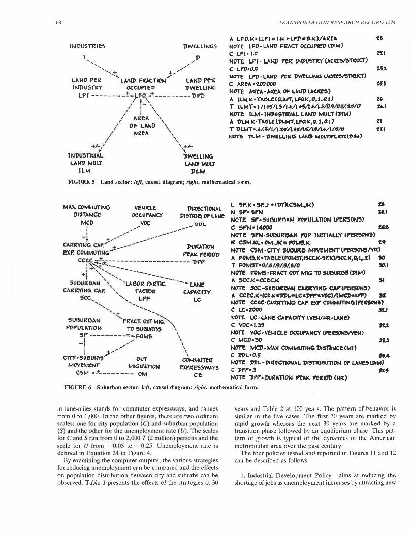
Figure 5 shows the land sector and the ways that industry and housing compete for land. Availability of land influences the expansion of industry and housing through the industry land multiplier (ILM) and dwelling land multiplier (DLM), respectively.

These five sectors will be considered as a system with inter­actions within and between the sectors. Job availability mod­ulates migration into and out of the area through an attrac­tiveness multiplier. Availability of housing also influences housing construction because builders and developers cannot make a profit by building and marketing houses for which there is no demand. Population and industry structures are

coupled through the ratio of labor force to jobs, population and housing through the ratio of households to housing, and industry structures and housing through values of the land fraction occupied.

A city is not self-sufficient. The hypothetical city must reach out into the hinterland for water, food, clean air, energy, and raw materials. Physical systems that help an urban population cat, drink , breathe, sleep, work , and move about are engi­neering systems. These systems are lifelines; without them, modern cities could not exist . Transportation is a life support system that can be superimposed on previously modeled socioeconomic systems.

Drew

USEFUL LIFC MOU'3t:MOL1> 11) C.ITY OF l>WeLLIN<i MOUSUJG OTIO J'OP'UUTIOH

UL')) JMR _.i-_________ CF"

l -1 L '', -l / : .... ,

T I I t',-J)WfLLING / M005CMOl.'P I 4,.ATTltM:TIVfWCS5

'PfMOLITIOtJ / Sl~e I MOUSINCr MU\.T. I I

"VJ)~ I M5 I AMM

I +', / I y ) - I ,1:'+

"PWfLLOJ&s 1'WtLL AVAIL. MULTlfLltlC

-PAM I I I

+~ l>WW.. CONSTlt

CONSTrtUCTION MULTl,Llelt 1'C~---------1'CM ++ +t I I : :

l>WfLL CO~TIC "PWCLL LANl> NORMAL MULTlt-Llt~

1'GN "PLM

67

L 1'.IC•.:P.J ~l1'T;(])C.Jl(.,;17P.JK) " N 1>•1'N IZ.I

NOTe l>•J)WtUING' (5TllUCTUrtf'5) C l>N•~f.000 IU NOTC W· l>WfLUWC.S INITIALLY(~TllUCTUrtfS) ll l)C.KL • J). I<,., J)CN •l>CM.I( " NOTt 1X: • 'J)WfLLUJG CONSTIZUCTION lSTllUC.Tf)'Jt) C l>CN • 0.0':1 ''·' NOTC 'l>CN-l>WtLL CONSTll NOR:MAL lFR:ACTl'tll) A ~M.K •:PLM.K•l'AM.K , .. MOTC 1'CM·J>WCLL CON5TR: MULT (PIM) S{ 1'J',l(L•1Uc/UL1' '' NOT? 17JJ • l>WeWNG 'MMOUTlDM (S'TlnJCT /'tX) C UL) • ""-C. "1- "·' NOTC UIJ'·U5tfUL U,.t l>WtLLING (Y)t)

A 1'AM.IC.•TAOLC(1'AMT,~Mlt.l(,0, ~.0.2) "' T l>AMT•.'L/.~,-l.ff/.IJl.~/l/1.'9/1.4./1.1/S.""2. "'·' >JOTt 1>AM ·~LU.,._ AVAILADILITY MULT (l>lt.0 A MMll.K• cr.l(/(1U<41 M~) IJ NC7Tt MMr< ·MOWtMOll' 1D MOU51NG llA.TIOO>IM] c "'5•4 If.I wcrrr ~. MOOHMOL'P 91ae C"1CION$/4&11n1CT) A AMM.K•TADLClAMMT.MMtr.l(',0,1,U) II T AMMT • U./1.4/f.J.'T/LJ/U~/1/.l/."'/.~/.U/.4- II. I NOTe AMM • ATTKACTM~ ~lt.IG MULTCJllM)

FIGURE 3 Housing sector: left, causal diagram; right, mathematical form.

LA OOrt PAltTIC. FRACTION

Lf F I

+t LABO!t FOstce

SUe\J"DAN POPULATION

'JP I I

l+ ,Or\JLATION

LF~~--------------------- , : t

+' ,+ LArsoJ FOrza ofv JO~ fU.TIO JOD5 l'Of'ULATION

L~J1t--=--------.Jt '- Cf'

I ++ .... +t l ,, T I '

INl>US. LAOO!t JOM f'Clt ', FOctct MULT. INl>USTrtY lNl>USTitle5

lLFM Jf"l I

A ILFM.l(•TAOLCULfhfT,&.FJrt.IC,0,2-,0.~) llf T l LF MT•. 2./. 2'1/.,,-/. f"l."111/1. "°/l.wl.&t/l.'ffl"L !CJ.I NC7Tf ILFM· IN1>~ LAeoR FORCt MULT('DIM) A LFJR.I( • LF.K/J,I(. 'ZO Nore LFJR:·LAOOSZ r=cmcr JOO ltATIO(l)IM) A LF.K• F.K•LrF- ii NCTR LF- LADOR: FO"ce C.l'eCON5) C LfF'• O.'° ti. I Nvrt &.rF- ueoc fAlfTtClfATIDN FllACT('JilM) A P:I(• Cf.IC+~r.IC. 2% NOT? F'- ,orOLATION 're~> A J"• 1.1<-tiJr'J Z3 Ncn't J•JOO~C.reno~) C Jrl•.,6 UI NOTe J~I - JOI» ~ l~ (t't~MJIUS) 5 UrtK• (LF.K-.19<:)/LF.K t~ won Ult-UNtM,.LDYMtfJT SQ.Te•(l)IM)

FIGURE 4 Employment sector: left , causal diagram; right, mathematical form.

If the availability of employment and housing is the prin­cipal determinant of in-migration to the hypothetical urban area, accessibility of suburban residences to central city work places (achieved through suburban expressways) accounts for the movement of people from the central city to the suburbs. The causal diagram and mathematical model for the suburban sector are shown in Figure 6 and for the transportation sector in Figure 7.

The causal diagram for the entire METRO model is shown in Figure 8. Streams of causality can be followed from variable

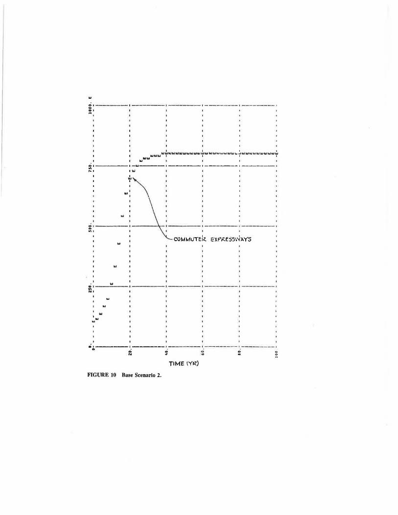
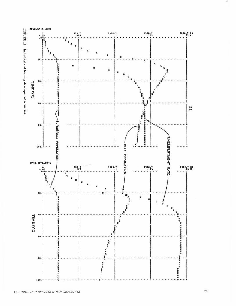
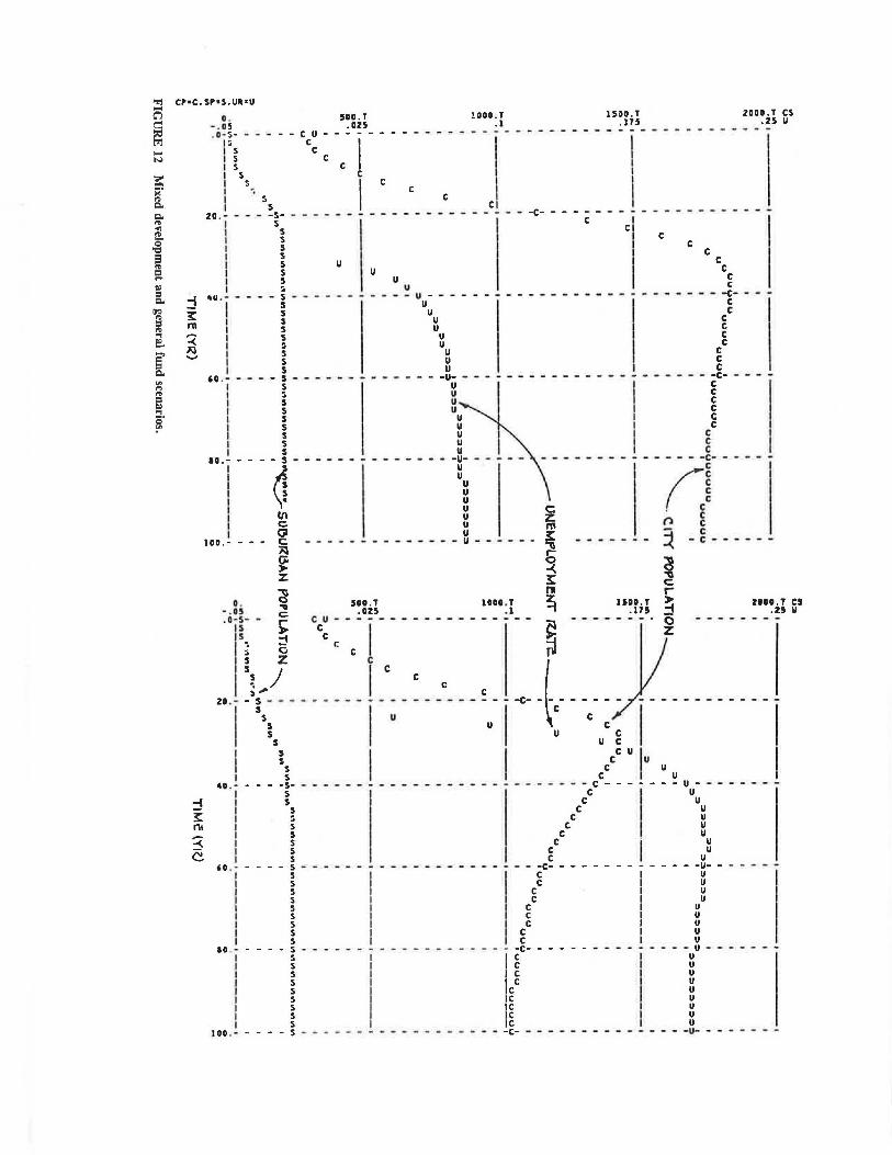
to variable through the sectors. The suburban population SP depends on the lane-miles of commuter expressways CE. Fig­ure 8 also gives the control statements for the model outputs, which are presented in Figures 9-12.

Figures 9 and 10 show the standard or base run outputs of the model. Figures 11 and 12 are outputs of alternative scenar­ios based on parameter changes made to represent various development strategies. In these four figures, the abscissas are time corresponding to 100 years in the lifetime of the hypothetical metropolis. In Figure 10, the ordinate E expressed

68

IN'DUSmlB l>WE:LLINGS

1) ', ,/

',, ,~ .......... ~ + ..........

..... , >"' LM-ID Pf~ LA-NP ~AC.TIOIJ LAN1' f'Elt 1 Nl>U~TJtY OCCUf'I f1' l'WE:LLING LPf--------t-LFO~~---------~n> , t ' / -\

I I ' I I '

I I ' / A~tA \

/ OF- LA"'1> \ / ~~e" \

I \ I \

+I- I '+,t-/ \

1NJ)U5nt1AL l>WfLLINGr LAN]) MULT. LAN) MUl.T.

ILM J>t.M

TRANSPORTA TION RESEA RCH RECORD 1274

A LFO.I<:• (Lf'l 11 I.Jc:+ U'J>•'l>.k:)/AefA NO'Tf: LFO • LA"'1D FllACT ~CUPlfl> ll)IM) C LPI• t.O HI NOTf LPI - L-'WD Pfl'l lWJ>U':ITIC'( (ACr.?~TINCT) c L.l'P• o.i; i1J.i NOTf Ll'l)- LA"'1> f'tR: 'PWeWNG lAiCIU~/5mUCT) C NteA • 1.JJOOOO ZU NOT'E AJZfA-Art.eA OF LAMPlA~) A ILM.K•TAOLZULMT,LFD.l<,0,1,0.IJ f(, T ILMT• l/1.1~/l.,/f..f./l . ..,A ... /U/D.CJ/O.,/.~"/O Z'C.I Nore lLM- lNPUSTlflAL LANJ> ~UJLT ('J)IM) A t)LM.K•TAOL.ell>LMT,LFO.K,O, l,O.JJ %1 T l>LMT•.4-/.~/l/1.~,-/l.'f'A.JIL~M/l/..,/O tU NOT'e l'LM -1'WeLLtwa LANI> MULTl,Llettlt'IM)

FIGURE 5 Land sector: left, causal diagram; right, mathematical form.

L ~~1<·5'-J +117TXCSM.JI<) a N Sl'•~'N UI NOTf Sr'-SUOOROA~ f't'f'UU.TIOt-! tf'eRSONS) C Sf'N• 14000 US NOTe ,f'N·5UOORr!AM POf' INITIALLY (f"!~N~) R C5M.l(L• OM.Jk• FOMS.K f.49 NOTe C'SM-CITY su,,..e MOWMrNT(~'/VI'() A FOM~.K • TAl!l.e lFO..eT.<5CCJC·S'-kV5CC.K,O, I,.%) 10 T FOM,T•0/.8/.9/.9/.8/0 50.1 NOTE! FOM!-FRACT OUT MIG,,, su~m(J)IM)

"" scc.ic:•ccec.1< 51 NOTe .SCC ·SU,,UICDAM CAlan'IMG CAP' C.meJDN5) A CC:fC.l(•(Ct.K•1'1>L•LC•1'rl'•WC>ltMCP•U'P) H i.iOTe ccec-CARRY!t..IG CAP' eVF' COMMllTINGrlf'e~) C LC•%000 .H.t NOTf LC- LANf CAf'ACITY (VfM/MR:-LANe) C VOC•I.~ JU NOTe VOC-\'e~ICLf OCCUl"ANCY' (P'e"50N~) C MCJ>•30 JU NOTC MCl>- MAX COMMUTING 'J)l!TANCf (Ml) C l'PL•O.f ,._ ... NOTe PPL - J)1~eCT10NAL 'J)l'11QOOTIOH OF LANf5 l'DIM) C Pf'~·3 Jt.9 NOTe "Pf'P-lXl~A,,OW f'eAI( ~IOD (MR)

FIGURE 6 Suburban sector: left, causal diagram; right, mathematical form.

in lane-miles stands for commuter expre ways, and ranges from 0 to 1,000. In the other figures, there are two ordinate , cales: one for city population ( ) and suburban population ( ) and the othe r for the unemployme nt rate ( U) . The scales for C and S run from 0 t 2,000 T (2 millio.n) per ns and the scale for U from - 0.05 to + 0.25 . Unemployment rate is defined in Equation 24 in Figure 4.

By examining the computer outputs, the various strategies for reducing unemployme nt can be compared and the effects on population distribution between city and suburbs can be observed. Table 1 presents the effects of the strategies at 30

years and Table 2 at 100 yellrs. The pllttern of behavior is similar in the five cases. The first 30 years are marked by rapid growth whereas the next 30 years are marked by a transition phase followed by an equilibrium phase . This pat­tern of growth is typical of the dynamics of the American metropolitan area over the past century.

The four policies tested and reported in Figures 11 and 12 can be described as follows :

1. Industrial Development Policy-aims at reducing the shortage of jobs as unemployment increases by attracting new

( COMMUTeJt ex r.

ltfVfNUB CEit

\. +\

\ \

' \ \ ' \ \

UNIT COtJSTl(. UNIT MAINT'.' COST CO~T

OCC OMC I I I I I I

-· ~+ MIGMWAY COMMUTER exr. FUN1) MAINTfNANC.t

. :iF ------CF COMMlJTC~ fXI'. COMMVTC.R

' \

co~~lJC'flOij EXrRC,5WAY5 CfC.----+~a

l +1

I I

F~AC.i FUNJ>

ALLOC~

FF1'

\

' UNIT R:e~NUf UNIT R:fYeWUf UNIT SltVfNUe exr. NOnfAl fXf'Re5,WA.,, exr. MULT.

tmeN---------4:.-uRe ~t-________ URfM

L Cf.K•CC.J +-tln?ICEC.JK) N Ce•CfN NOTe Cf-COMMUTf~ Ellrr~e55WAYS (LANe Ml)

C CCN = 100 311 NOTt CfN-COM fXF'lt~SWAYS INITIALLY lLANe Ml)

R CEC.KL•(l.U~.l</IJCC)•FFA 34

NOTC CfC - COM fXr' CCNSTltUCTION lLANf MI/YR) C UCC • '%000000 34-,I NOTe UCC - UNIT CONSTS:UCTION COSTl t/LAN f M 0

C FFA•l.O ~.i

Non~ FF.&.-FR'ACT FUND ALLOCATl':'D(F~ACTIV~) L MF:I< • MF.J +fPT)(CeR.Jl<-CfM.JK-CfC.J~• UCC/FFA) 3' C MF•O 3!:U NOT? HF-MIG~AY R."1> (t) R CeM.KL•Ce.K•Ut.tC 3(., NOTC CEM-COM fXr' MAINTCNAIJCe lf/Ylt) C UMC • tOOOOO 3'.. I NOTC UMC-UNl1' MAIWT?NANCC CO"ST(t/Ylt-LAIJf Ml) R ceR.KL•Cf.l(«U~e.K 3; NOTe CeR -COM exr" "eveNUI:' ltl'Vit) A Ultf. K • URfN • UR:eM. IC ~ NOTe U«f·UNIT R'eV EJCP'Re55WAYS (~·LAMC Ml)

C llReN "''00000 31$.1 NOTe USlfN -UNIT RCV EXf' NONAL l•l'Vll-LANC Ml) A UrfeM.IC•T-"'Lf (Ullft.rT,ce.K,0,1000,100) 3' T USleMT• 0/1/1.~/I. 3/1.111/. 6/.4./. 5/.4/.'/. 2. 39.1 NOT'e urteM- UNIT ltt\' ~,. MULTIPl.lflt (PIM)

FIGURE 7 Transportation sector: left, causal diagram; right, mathematical form.

PLOT Cf'•C,'Sr'•S l0.2000000)/UI(• U l-.OS' .. ZO) NOTe C-CITY .-VPULA.llON NOTE s-sueuitoAN F't>VULATION NOTe U-UNeMP'LOVMe-NT R.&.Te F'LOT Cf•El0,1000) NOTe e-COMMUTelt ex~e5SWAYS C 1'T•D.~ NOTf 1'T· 50LUTICN lNTf~AL lvrt) c LeN"n1 • ~o NOTC LCN<.TM-Lf:NwTM Of' ~IMULATIO...i lVIC) C PLTnlC•I won f'LT,fl(- F'LDT P"eCturo C JC.M•0.15 NOTe. lNCJU:>.'e It.I lC:.IJ FllOM O.tO TO o.1e SflJN (tJl)IJSTltlAL 1'f:VfLOf'MftJT SCft.1.t.ll!IO C 'lX:N•0.10 NOTE: INCl(fA~e IN "PC.N ~ .... o.o; TI> 0.10 RUN MOUSltJG 'J>CVf.LOf'Mf:t.IT SCeNAR:IO

C IC.N•0.15

C UL1'•3',, NOTC CMANGC~ IN ICN ANl> UL'J) RUN Ml)(C'J) l>CVC'LOPMCNT SCt:IJAr<:IO

C FFJ.•0.~ ~OTC CMt.Ncae IN FFA F~OM 1.0 TI) O.'i

RUN GENf~AL FllN'D SCfNAR'IO QUl1'

FIGURE 8 METRO model: left, causal diagram; right, control statements.

FIG. 9

FIG. 10

FIG. 11

FIG. 11

FIG. 12

FIG. 12

.. U:>

~ .. •"! ·------­a • "'

I ~ .. .... , ... a• I ,,.

IU

I -.. u . ··-------· • • a

_,,, I

·NI •• a• I ~

CITY u

u

u

u ____ , _,. ____ _ u

u

u

~IJBUl:t.l~AN f'OPULATION1~ : :

I I I I

t ~~~~~~~~~~~~~ .... ~~~~~M~ "'M~~~M..,M~~ .... MMW"IMMM ,,,.,, "'' "' ,. "' . .. .. "' ~ . .,, ........

""'"'"' M DO I-------I -------1 -------1 ------1 ------1 " •G • • • • A. I • 0 0 e G D .,, "" ,. _. • a u ~ TIME l't'~)

FIGURE 9 Base Scenario 1.

"' 0 I-------• ----·----I - ----- I - -------I --------- • D 01

DI

"' .... ----1 -w-----I-------I------- I-------- t

··----D

"''

...

"'

..

...

, ... .:. I

I ... I

01-------"' NI

I ... ...

... ...

...

---- I------->

COMMUTCll. EXf'Jl..f~S'."AYS

'------·- I--·---- j

0 I ------1 -------I------·-- f ---- - ---I --- ·- - --I 0 • . • •

• N

FIGURE 10 Base Scenario 2.

TIME \Y~)

0 .. .. ..

"1 C'•C , S,•S,UR•U

~ .... .... .... = Q. = "' [ § Q.

:r g "' a=g· Q. .. ~ .g

~ ~ ~· '!'

0 . -. OS .o-s-

ID~O . T . l

UOO.T .175

2000.T CS . 25 u

-i ~ l'Q

~

1\ I :; I s I s I 5s I I zo .-1

I

SS -s- -

SS s s s s

c c

c

u u

u

40 . -1

~s - - - - - - - - - - - - - - - - -- - - - s

I

"l 10 .-

100 .- - -

s s s s s

l I -------l - - - - - - - - - - -- - s s

,~ II\

~ :N ~ > z

~ c

~ 6 %

- ~ - - - c - - c

u u

c c

c c c

c u I c u c

-u- - - - - - - - -c- - - - - - - - -u c u c u c u c u c u c u c

U Cl u c I

- - - - - - - - -u- c - - - - - - - - - - - - -UC c c

cu cu

c u c u c u c u

- - -ri--- -g-~ - -c u c u

c u c u c u c u c u

n

~ ~ ~ .-

c u -c--u--

c z m ~ "'Q r-

~ "' z -i

cu cu

ct'•c,s,•s,u•·u; 0 .

- .n SOO.T .ozs 1000. T

.1 ~ 0 z

1500. T . 175 ~

HOO. T CS .HU

.o-s- - - - - c u -Is c

s c I s I S I s\; s I s

zo .- - - - -s- - - - - - - - - - - -

c

- u -

c c

c c

c j I I c - - -c- - - - - - -

I :;

I l I s I ~ I s I s I s

I UC

I ) I g I cc

u

-i ~o . - - - - - s - - - - - - - - - - - - - - - - - -- I s

- - -c- - -

I c{ ~ I l m I S

~ s s s s s

IC c c

c'I

u

"'

u u

u u u

u - - - - - - - - u - - -u

u u u u u u u u

'° · -s -- - -- - - - - - - - - - - c - - - - - - - - - - - - - - - - - - . - - - - u -

I ao .-1 I I I I

I

s s s s s s .. $ s s - - - - - - - - -s s s s s s s s s

c I

~ I c I .c I

c I g I

C I - - - - - -c- - - -

( I c I C I

~ I

u

u u u u u u u u

- - - - - - - -u- - -

u u u u u

u u

" u

I 100 . - s - - - - - - - - - - - - - c - - - - - - - - - - - - - - - - - - - - - - - - - u -

f!Lll mIOYJN H:JNV3S3N NO/.LV.LNOJSNVNL u

::.1

~ .... N

f. .. =­=­.. ~

'O

~ 5!.

i ~

~ 8' a. ~ = el ~·

CP•C,SP•S,UR•U

o. -. 05 . O- ':>- - - - - -

I :i I S I S I S l s I s

I 20 .-

1 I I I

I

-. s s -s-s s s s s s s s :i

c u c c

500.T .025

c c I l

u

c c

u u

u

c

!000.T . l

c - - -c- - - - c

15DD. T .115

cl c

c cc

c c c

2000.T CS .Z5 U

j <ou . s s

u u u

- - - - - - - - 1-c

c c c c

~ m ':<: .IQ ......

~ 3:: "' ::z c

'°·

ID. I

I I

I I I I

100.-

s s s s :; s s s

- s s :i s s s s s s s

- s

d C/I c (j1 c:. ;;i GO > z:

u u u u u u u

- - - - - - - - - - - - - -u- -u u u u u u u u u

- - - - - - - - - - - - - - -u- - - - - -u u u u u u u u u

- - - - - - - - - - - - - - u - - - - - -

c: z "' ~ ~ 3::

c c c

- -c-

c c

c c c c c c

_g_ - - - - -c

r:~ c

('l c

~ ~ ~ r

- g - - - - - -

1000. T ~ ~ 500.T : l _ - ~ 0 , . 025 - - - - - - - - - - >: _. o! c c u - - - -

1

- ::.-t

. Di~~ - ~ CC r. C ~fll 1500. T

.115 ?j 0 z

ZODO.T CS .25 u

.• 0 c

l z ' ' - ---s ; I r. c -------- -7! ! -------- --< ' / )~ ----- - I cc -s-- -- --- I u u u c

s u c

$ c u I . ' ' ' . ' ' s~ I ---! -------/- ------\ ' --- --- ' ' ' --- ---- ' ' -·- - - ' ' ' ' ' 5s c ., ~ ' ' ' - - -s I c ___ -u- - - -' ' - - - - - - - ' ' - - - _,_ - - I ' l - - - - - - - - - - - - - 1 I ~ >- -- - - ' I '

' ' I ' ' < I ' ' ' I ' s ! c I u - --· ' ' , ____ , __ _ s c ----- --, u ' - -<- - - - ' s I --------- IC II u ' ------ ' ' • --- I ' '

' I < ' ' ' ' s c I u

' ' ' - -- --' ' - - - _,_ - -s c - - - - -i -------------------c- - - - - - -

20 . -

I I

I I •o .-I I

I I I I

60 . -I

I I I I I I I

ID • I l I

I I

I I

I 00 . -

74 TRANSPnRTATION RESEA RCH RECORD 1274

TABLE 1 COMPARISON OF SCENARIOS AT TIME T = 30 YEARS

f!;!,ram~:t~Cli! El~§~ rum E2l1S<::l ;i. foJ.1soll: ' f2Usc:ii:: ~ f2il~x ~I ICN .10 .15 .10 .15 .10 DCN .07 .07 .10 .07 .07 ULD 66.7 66.7 66.7 33.3 66.7 FFA 1.0 1.0 1. 0 1.0 0.5

CP 1430T 1719T 1190T 1766T 1424T SP 212T 212T 212T 212T 147T UR 0.14 0.09 0.20 -.02 0.15

TABLE 2 COMPARISON OF SCENARIOS AT TIME T = 100 YEARS

f~Cli\ID!i::t!i:Cli! Base BYD fQliS<ll: ICN .10 .15 DCN .07 .07 ULD 66.7 66.7 FFA 1.0 1.0

CP 1026T 1295T SP 216T 216T UR 0.20 0.16

industries, accomplished in the model by increasing industrial capacity initial value (ICN) .

2. Housing Development Policy-represents a strategy (i .e., low-income housing programs of the 1960s) encouraging the construction of more housing, accomplished in the model by increasing dwelling construction initial value (DCN) (Figure 3, Equation 13.1) .

3. Mixed Development Policy-represents a combination of increasing ICN as in the industrial development scenario while reducing useful lifetime of dwellings (ULD) to remove slum housing .

4. General Fund Policy-corresponds to using the highway fund for nonhighway purposes, a proposal that surfaces from time to time. Indeed, it has become commonplace to divert highway earning to transit subsidies. This policy is imple­mented through the parameter FF A in the model (Figure 7, Equation 34.2).

On the basis of the unemployment rate as a measure of effec­tiveness, development alternatives can be ranked from best to worst in this hypothetical case as follows: Policy 3, Policy 1, base policy, Policy 4, and Policy 2 (see Tables 1 and 2).

MODELING REGIONAL AND NATIONAL ECONOMIES

National development models should, ideally, be structured to accommodate three development orientations: (a) resource development, (b) regional development, and (c) sectoral development. Resource components include natural resources, land resources, water resources, and human resources (man­power). Regional development is organized on the basis of rural and urban. Sectors represented in the model are agri­culture, manufacturing, business, infrastructure, and govern­ment . Obviously, the three orientations overlap and are also tied together by two quantities most responsible for material growth: (a) population, including the effects of all economic

l. fQliS<ll: 2 fQliS<ll: ;l foliS<:ll: ~ .10 .15 .10 .10 .07 .07

66.7 33.3 66.7 1. 0 1. 0 0.5

798T 1754T 1013T 216T 216T 216T 0.23 0.08 0.20

and environmental factors that influence human birth , death, and migration rates; and (b) capital , including the means of producing industrial, service, and agricultural outputs.

Many of the sectors of a national or regional model can be thought of as elements in a national account that is con­cerned with measuring aggregate product originating within some geographical area to provide a picture of economic performance.

End results of economic activity are the production of goods and services and the distribution of those goods and services to members of society. The most comprehensive measure of national output is the gross national product (GNP), which is the value of all goods and services produced annually in the nation. Estimating GNP, however, is not merely adding up the value of all output because that would result in double counting. The value of any product is created by a large num­ber of different industries with each firm buying materials or supplies from other firms, processing or transporting them , and thus adding to their value.

Four major components of GNP, each representing a final use of GNP, are consumption, investment, government pur­chases, and net exports. Investment refers to that portion of the final output that takes the form of additions to or replace­ments of capital. Government purchases of goods and services are a second component of GNP . In addition, government makes other expenditures in the form of transfer payments, which do not represent the purchase of output and conse­quently arc excluded from GNP. CuJJsumplion refers to the portion of national output that is devoted to meeting con­sumer wants. Net exports (exports minus imports of goods and services) are a final use of GNP and must be included in the total. Three of the four major components (consumption, investment, and government purchases) can be grouped under the heading of gross domestic product (GDP). The GNP, then, is the sum of the GDP plus net exports.

For purposes of national income analysis, GNP statistics are subdivided into mutually exclusive, collectively exhaustive categories. The most commonly used scheme for subdivision

Drew

is based on the International Standard Industrial Clas­sification (ISIC). The nine major ISIC categories are as follows:

Code Classification and Description

1 Agriculture , hunting, forestry, and fishing 2 Mining and quarrying 3 Manufacturing 4 Electricity, gas, and water 5 Construction 6 Wholesale and retail trade, restaurants, and hotels 7 Transport, storage, and communication 8 Financing, insurance, real estate, and business services 9 Community, social, and personal services

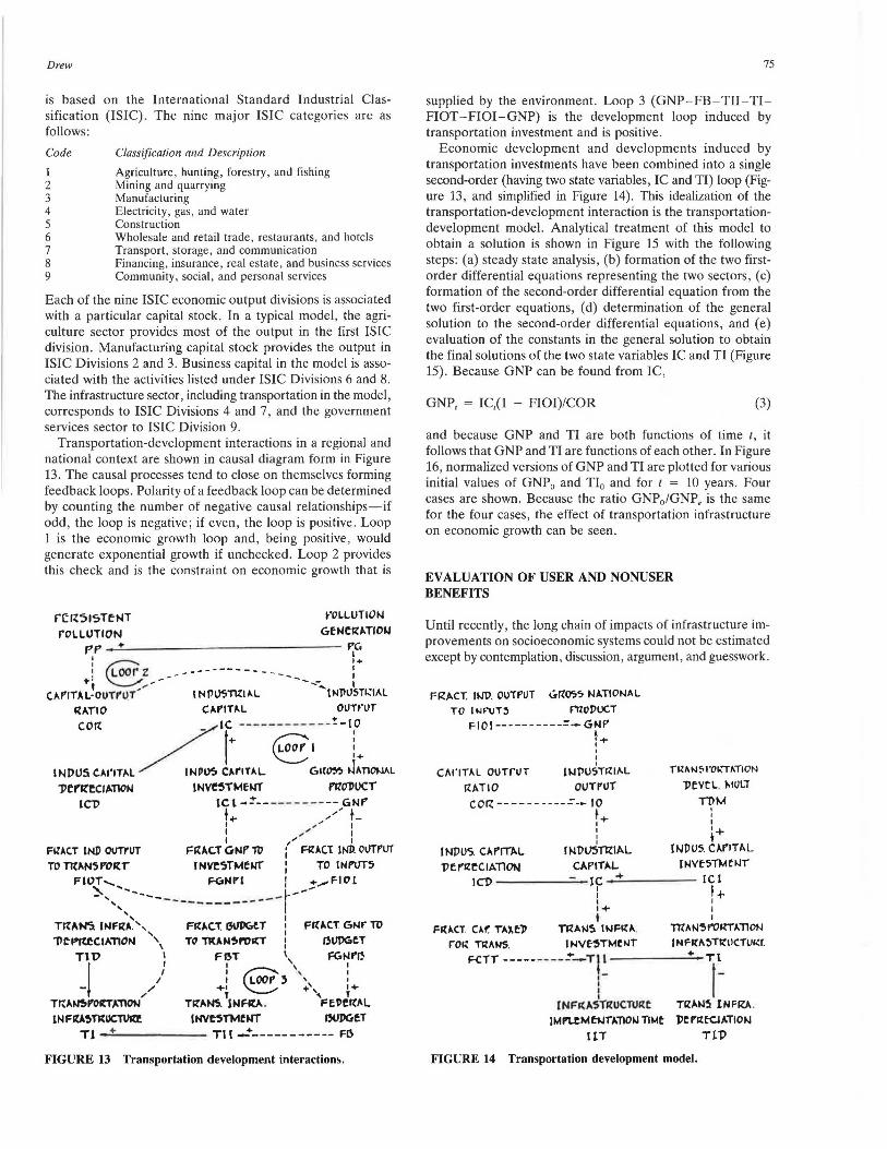
Each of the nine ISIC economic output divisions is associated with a particular capital stock. In a typical model, the agri­culture sector provides most of the output in the first ISIC division. Manufacturing capital stock provides the output in ISIC Divisions 2 and 3. Business capital in the model is asso­ciated with the activities listed under ISIC Divisions 6 and 8. The infrastructure sector, including transportation in the model, corresponds to ISIC Divisions 4 and 7, and the government services sector to ISIC Division 9.

Transportation-development interactions in a regional and national context are shown in causal diagram form in Figure 13. The causal processes tend to close on themselves forming feedback loops. Polarity of a feedback loop can be determined by counting the number of negative causal relationships-if odd, the loop is negative; if even, the loop is positive. Loop 1 is the economic growth loop and, being positive, would generate exponential growth if unchecked. Loop 2 provides this check and is the constraint on economic growth that is

re~515TtNT

roLLUTION

fOLLUTIOt.I GfNC~UIOIJ

PP + ~

l rloOr z ------------- -- -- !+ +t ~ .... ,- --- I O.F'ITAL·OUTl'l)T ' INPUSmt~L ... INJllJSTl.'.IAL

~ATIO CAF'ITAL oun·ur

COR /}-----e~- -'-li. lNPU!i C.M'ITAL / INll~ CArtTAL GI(~ ~ATIOW.L 1'frl(~Cl~TION lNV~Tt.1Em- PJtl11)UCT

lCl) lC l -~-- ------- -- GNf' ++ ,,.,.- L

FllAC.T lNl> OUTrllT TO mAN5f'OR:T

I ,"" I I ~ ' I I ,,,. I

Fll:AC.T GNP 'ft) I RAC.t 1NI>. OllTPUT tNVC~TMfwt" : TO lNf'UTS

FIOT, F<:oMl'l J +,....Fl 0 l ~' .. ____ - 1----

',, - ------- --- - -- I TrtANS INFR:A~', Frt1'C.T. G\IPGf.T I FttAC.T GNr TO

' I 1'C:Pft.CCl-'TICN \ TO TIUN~n:>ICT I ,,Vl)GCT Tl'D I FBT \

l I I '

I : r.;;:;;.'!J ',,, I

- /I +j ~ +"' ~+ Tl\A~rolCT,&.'TION T~,t.NS. lNFSV. . Ftl>ettt.L 1NF6~TR:UCT\lltt INV~TMfllT OOJ)GtT

Tl + Tl I_: __ _________ FB

FIGURE 13 Transportation development interactions.

75

supplied by the environment. Loop 3 (GNP-FB-Til-TI­FIOT-FIOI-GNP) is the development loop induced by transportation investment and is positive.

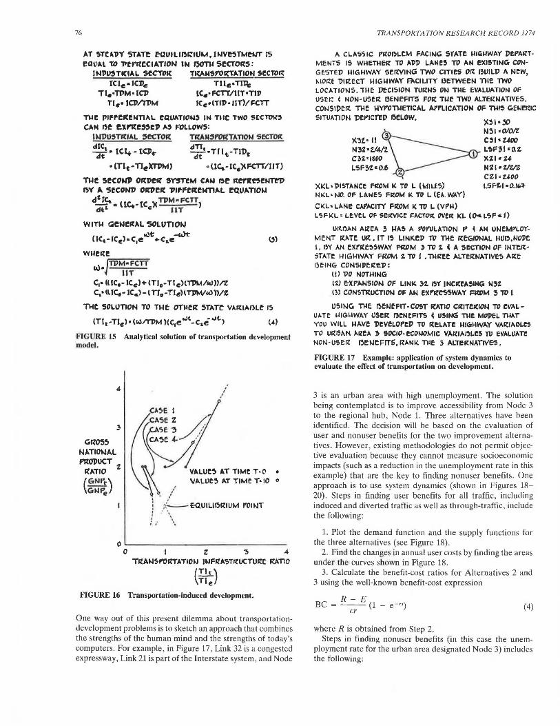
Economic development and developments induced by transportation investments have been combined into a single second-order (having two state variables, IC and TI) loop (Fig­ure 13, and simplified in Figure 14). This idealization of the transportation-development interaction is the transportation­development model. Analytical treatment of this model to obtain a solution is shown in Figure 15 with the following steps: (a) steady state analysis, (b) formation of the two first­order differential equations representing the two sectors, (c) formation of the second-order differential equation from the two first-order equations, (d) determination of the general solution to the second-order differential equations, and (e) evaluation of the constants in the general solution to obtain the final solutions of the two state variables IC and TI (Figure 15). Because GNP can be found from IC,

GNP, = IC,(1 - FIOI)/COR (3)

and because GNP and TI are both functions of time t, it follows that GNP and TI are functions of each other. In Figure 16, normalized versions of GNP and TI are plotted for various initial values of GNP0 and TI0 and for t = 10 years. Four cases are shown. Because the ratio GNP0 /GNP, is the same for the four cases, the effect of transportation infrastructure on economic growth can be seen.

EVALUATION OF USER AND NONUSER BENEFITS

Until recently, the long chain of impacts of infrastructure im­provements on socioeconomic systems could not be estimated except by contemplation, discussion, argument, and guesswork.

F~ACT. tt.ro. OUTPUT ~nos-; NATIONAL TO I Nf'UT ~ f'IWJ)UC.T

FIOl----------=-GNP l :-+-

Cfll'ITAL OUTrllT

RATIO

' I llJ~USTlllt\L

ounur ,..~,.N~roi..-n.T10N

1'eVtL. MULT

corz----------=-~ 10 ~M • -+' I I I

: ++ INPUS C>-f'ITAL twuu5m1AL lNDUS. CAPITAL l'CF'llCCIATlOlll CAPITAL (MVE-Sn.mJr

!CD -------le _ + _____ lC l : I+ I I 1+ I I I

TRAM~ l~FllA . ~AM~t'ORTAllON

ro" TllANS. INVE-:STMO.IT JNFKfl:>TKllCIUi.:r.

F<:TT --------- .:+°'- Tl 1------'-+..- Tl

I- I-I I

(NF'KASTIWCl\Jllt T~AM5 INFSV.. IM~MbJT"AllOtJ llMt J)tl'ltK:JATIOt.I

UT Tl1'

FIGURE 14 Transportation development model.

76

AT STCA1'Y ~TATt ~UILIDl:IUM. HIVE5TMf1JT IS eQt:AL TO "PfrRfCIATION IN DO™ StcTORS:

IN1'U,TKIAL seCTOK TKAMSl"OltTATION SfCTOR

ICle•ICDc Tle·TPM• ta>

Tie• ICl>./TIIM

Tlle•TI~ lCc• FCTT/I IT •T11) ICc•lTIP• llT)/FCTT

Tiie Plf,.Cftl!NTIAL eQUATION:I IN TllC TWO 5C:CTO~' CAN ~e Clt'lle,,ep .-.,, FOLLOWS:

1~1'U5TKIAL ,f'CTOR TRAN,f"OftTATIOM 5e<:TOI(

dTl, -·Tflt·TID~ dt

"'U'°'·IC.'XFCTT/JJT)

TMf secoNP Orl:l)tt SY'STCM CAN ~~ Ret'K~l!NTn>

BY A secoNl' ooesc PtrFerteMTIAL eal11.T10..i dtrc_ • UC.·tC .')( TPM,.FCTT) dt' e llT

WITM wewe"AL SOLUTION 143t -Wt'

(IC.·1Cel•C1e +C,e

wMeite w·J-=,,,,,,,..,...M.,... .. ""F""c""rr=

llT C1• lt IC.-ICc)+ tTl0 • Tte)(,,,,.1/w))/Z ~·l\JC,- IC.l-t TJ0 -TleHTPM/14)})/Z

THe SOLUTION TO TJ.U: OTMfR sr.t.n VA~l,t.DLf 15

(Tl tJC. -..it t•Tlel•(l.>ITl>M)lC,e -C~e ) (4)

FIGURE 15 Analytical solution of transportation development model.

4

G~055

NATIONAL PRODUCT

R1'TIO %

(GNl"r) GNPe

0 5E I CA':JfZA ..

~~:? / ~ -

' , .'

• Vl>.LlJC~ AT TIMC T• 10 o .

' ,

l . ;\.::__EQ.UILl0r{IL'M l'Ol!llT ' .. I '

f / \\

0'-------------- ----0 I Z ~ 4

T~Ai.JSl"OllTATIOIJ ltJF~A'I!Tlt'OCTUl<f ~TIO

I!!!.) \Tle

FIGURE 16 Transportation-induced development.

One way out of this prt:sent dilemma about transportation­development problems is to sketch an approach that combines the strengths of the human mind and the strengths of today's computers. For example, in Figure 17, Link 32 is a congested expressway, Link 21 is part of the Interstate system, and Node

TRANSPORTA TJON RESEARCH RECORD 1274

A CLA<;,51C l'IW~LCM FACltJG STATf: HIGHWAY J)f:f'AllT­MENTS I~ Wl-lfTMffC TO A'PJ> LANf5 TO AN E-XISTING CON­Gf:STEl> MIGMWAY SC~ING TWO CITICS O~ 5UIL1' A NCW, MO~f 1'1~fCT MIGMWAY F>.CILITY BfTWffN lllf lWO LOCATIONS. TMf: ]}f-Cl510N TUr<:NS ON TMf: EVALUATION OF user.: ~ NON-lJSfR: DfNCFITS FO~ TMf 'TWO ALTEIUJATIVfS. COl-ISIJ)f:~ TMf HYf'O™fTICAL Al'f'LICATION OF TMI~ C.Et.IC!l:IC SITUATION l>fPICTED BfLOW.

)C.~1·30

N~l •0/0/Z C~l•UOO

__ -/:',_ L~F:5t so.t Xtl • t4 Ni I • tltlZ CZl=UOO

XKL • l>l~TANCf FIWM I( TO L ( M1Lf5) L5fZ.l •0.1"1-NKL •NO. OF LANES FR:OM K TO L- (EA. WAY)

CKL•LANe CAf'ACITY FrtOM K TO L (VPM) LSFKL = LE:VfL OF- SEICVICf f::ACTOIC OVER: KL (0"5. L";f' I)

URr.>AN />.!ZEA 3 MAS A POl'ULATION P 4 AN Ui.lf:MPLOY­MeNT ~ATC lJR. IT I'; LINKC1> iO llff R:fGIONAL MlJO,NOPC I, ~.,. AN cxritf:55WAV FCWM ) TD 1 ( A SCCTION OF IMTeR:· -ST,t.TC MIGHWAY' FIWM t TO t • llf~Ef />.LTfll:NATIVE-5 Altf fjf:ING CONSIJ)f;~CJ:I:

ll) 1'0 NOTl41NG-l1} E'XP.A.NSION OF LINI'. n ~'( INCICeASING N'3Z m CON5TltUCTION OF AM fl<l'rt~SWAY FR.OM 3 lt' I

lJ51NG Tllf ~fl-If-FIT-COST ~TIO CR:tTfltlON TO fVAL-UJ. Tf l-llGl-IW,t.Y oseit 13fNCFITS ~ USI~ TMf MoPEL THAi YOU WILL MAVf; 'J)CVfLOl't1' TO IU.:LATf MIC:.MWAY V,t.l~IAOU"; TO u~~AN .a.izeA ~ 50C10-fCOt.IOMIC VArtl."1)LfS TO fVALU,t.TC NON-USE:!<: OetJfFrTS, ~ANI<. Tilf 3 ALTl!rl:t.IATIVES.

FIGURE 17 Example: application of system dynamics to evaluate the effect of transportation on development.

3 is an urban area with high unemployment. The solution being contemplated is to improve accessibility from Node 3 to the regional hub, Node 1. Three alternatives have been identified. The decision will be based on the evaluation of user and nonuser benefits for the two improvement alterna­tives. However, existing methodologies do not permit objec­tive evaluation because they cannot measure socioeconomic impacts (such as a reduction in the unemployment rate in this example) that are the key to finding nonuser benefits. One approach is to use system dynamics (shown in Figures 18-20). Steps in finding user benefits for all traffic, including induced and diverted traffic as well as through-traffic, include the following:

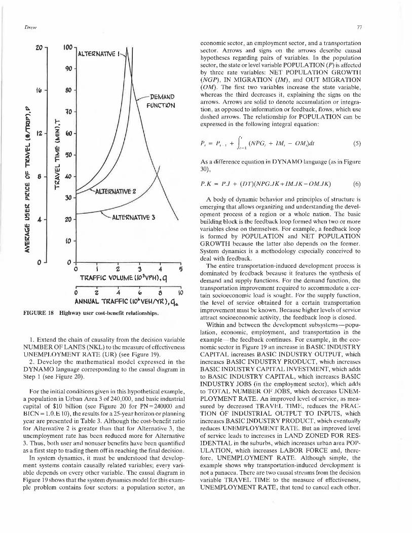
1. Plot the demand function and the supply functions for the three alternatives (see Figure 18).

2. Find the changes in annual user costs by finding the areas under the curves shown in Figure 18.

3. Calculate the benefit-cost ratios for Alternatives 2 and 3 using the well-known benefit-cost expression

R-E BC= -- (1 - e-")

er (4)

where R is obtained from Step 2. Steps in finding nonuser benefits (in this case the unem­

ployment rate for the urban area designated Node 3) includes the following:

Drew

to 100 Al TErlNATl\1€ I

90

l<o 80

~ 10 ,,...: ~

~ ~ ,....

12 z

"° • ~ -- --_J w ~ ~ '50

~ F ...J

LL UJ C) 8 ~ "'° Ul tll u I-

~ 30 t::l ILi Ill

ALTE'~NATIVf 3 :> .4. zo II.I

~ t:l 10 ~

0 0 0 I 2 3 4 '3

TRAFFIC VOLUME: uo>vrH),q

0 z 4 " 5 10 ~NNUAL TRAFFIC l 10" VE~/YR), C\~

FIGURE 18 Highway user cost-benefit relationships.

1. Extend the chain of causality from the decision variable NUMBER OF LANES (NKL) to the measure of effectiveness UNEMPLOYMENT RATE (UR) (see Figure 19).

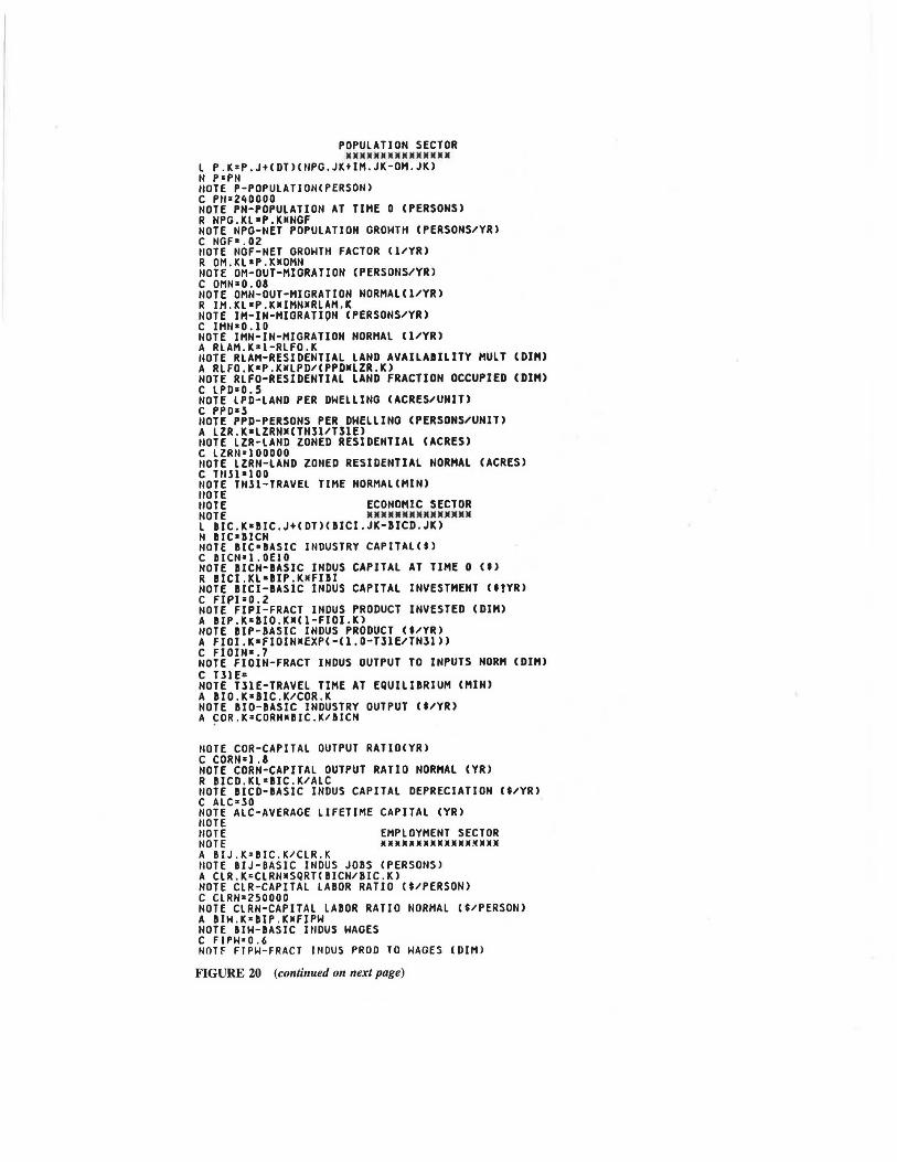
2. Develop the mathematical model expressed in the DYNAMO language corresponding to the causal diagram in Step 1 (see Figure 20).

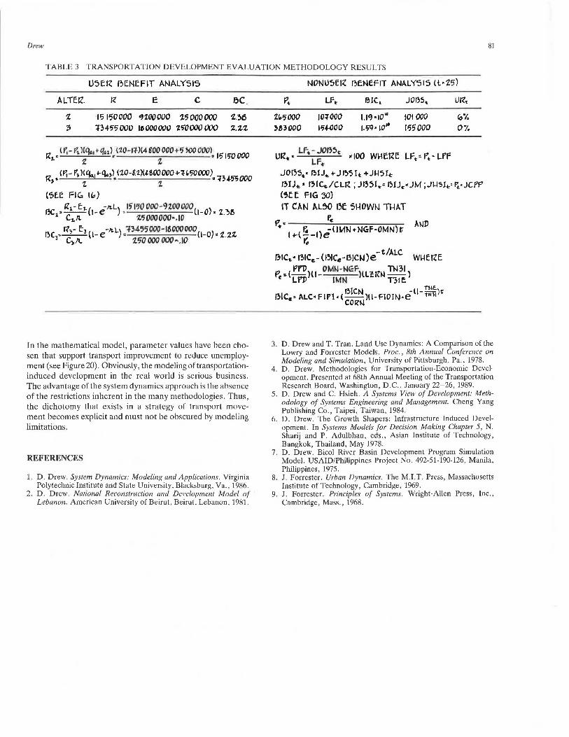
For the initial conditions given in this hypothetical example, a population in Urban Area 3 of 240,000, and basic industrial capital of $10 billion (see Figure 20 for PN = 240000 and BICN = 1.0.E 10), the results for a 25-year horizon or planning year are presented in Table 3. Although the cost-benefit ratio for Alternative 2 is greater than that for Alternative 3, the unemployment rate has been reduced more for Alternative 3. Thus, both user and nonuser benefits have been quantified as a first step to trading them off in reaching the final decision .

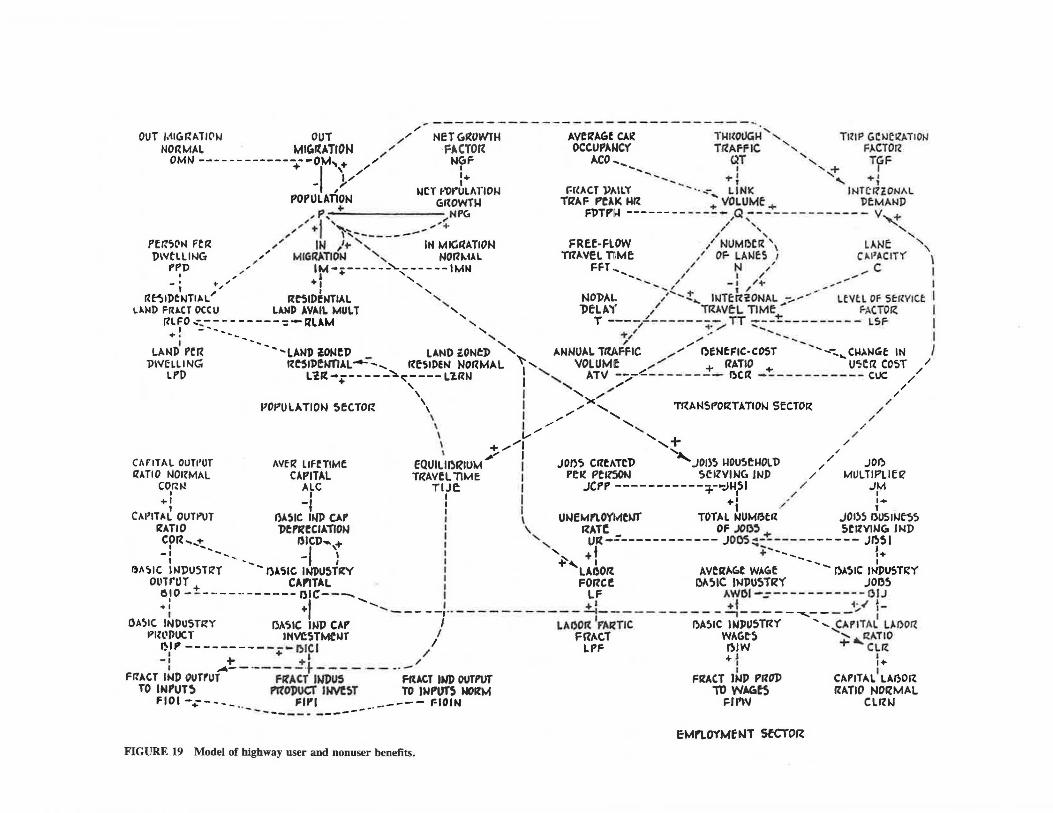
In system dynamics, it must be understood that develop­ment systems contain causally related variables; every vari­able depends on every other variable. The causal diagram in Figure 19 shows that the system dynamics model for this exam­ple problem contains four sectors: a population sector , an

77

economic sector, an employment sector, and a transportation sector. Arrows and signs on the arrows describe causal hypotheses regarding pairs of variables. In the population sector, the state or level variable POPULATION (P) is affected by three rate variables: NET POPULATION GROWTH (NGP), IN MIGRATION (IM), and OUT MIGRATION (OM). The first two variables increase the state variable, whereas the third decreases it, explaining the signs on the arrows. Arrows are solid to denote accumulation or integra­tion, as opposed to information or feedback , flows, which use dashed arrows . The relationship for POPULATION can be expressed in the following integral equation :

pl = P, _, + f I (NPGI + IM/ - OM,)dt r - 1

(5)

As a difference equation in DYNAMO language (as in Figure 30),

P.K = P.J + (DT)(NPG.JK+IM.JK-OM.JK) (6)

A body of dynamic behavior and principles of structure is emerging that allows organizing and understanding the devel­opment process of a region or a whole nation. The basic building block is the feedback loop formed when two or more variables close on themselves. For example, a feedback loop is formed by PO PU LA TION and NET POPULATION GROWTH because the latter also depends on the former. System dynamics is a methodology especially conceived to deal with feedback.

The entire transportation-induced development process is dominated by feedback because it features the synthesis of demand and supply functions. For the demand function, the transportation improvement required to accommodate a cer­tain socioeconomic load is sought . For the supply function, the level of service obtained for a certain transportation improvement must be known. Because higher levels of service attract socioeconomic activity , the feedback loop is closed.

Within and between the development subsystems-popu­lation, economic, employment, and transportation in the example-the feedback continues. For example, in the eco­nomic sector in Figure 19 an increase in BASIC INDUSTRY CAPITAL increases BASIC INDUSTRY OUTPUT, which increases BASIC INDUSTRY PRODUCT, which increases BASIC INDUSTRY CAPITAL INVESTMENT, which adds to BASIC INDUSTRY CAPITAL, which increases BASIC INDUSTRY JOBS (in the employment sector), which adds to TOTAL NUMBER OF JOBS, which decreases UNEM­PLOYMENT RATE. An improved level of service , as mea­sured by decreased TRAVEL TIME, reduces the FRAC­TION OF INDUSTRIAL OUTPUT TO INPUTS, which increases BASIC INDUSTRY PRODUCT, which eventually reduces UNEMPLOYMENT RA TE. But an improved level of service leads to increases in LAND ZONED FOR RES­IDENTIAL in the suburbs, which increases urban area POP­ULATION , which increases LABOR FORCE and, there­fore, UNEMPLOYMENT RATE. Although simple, the example shows why transportation-induced development is not a panacea . There are two causal streams from the decision variable TRAVEL TIME to the measure of effectiveness , UNEMPLOYMENT RATE, that tend to cancel each other.

,,-' ----------------- -------------. ....... OUT MIGr.l<TICllJ OUT ,,-"' NET GIWWTH AVe~AGf CA~ TMICOIJGM ' TlllP GC>Jl:~l<TIOIJ

NORMAL MIGrtATION ,,. ·FACTOR OCCUPAWCY TrtAFFIC ', F>.CTO~ OMN --------------~OM ,,-"' NGF A.CO... QT ', TGF

+ I .... ,+ ,,, • ... ... .. • ' + r I// I+ ........ '+'l ....... ,.. Tl

- I ......... ' ~ t

n/ wn 1-'0t•UllfflOl.J Fr(ACT l>J.ILY .... --... LINK '"'TCl7ZONJ\.L

POf'ULA ON GltOWTM TRJ.F PeAK Mrt VOLUME 'l>tMAND P + NPC. Fl>Tl'M -----------~- Q---•----------- V _,.,, I', ..... '~ ,' ', ~ ,, + ,.... _, ~ ' ' , ,, .. ______ " ' '

Pfr.<;ON FCR / IN /+ ', I,. MIGaATION FRff·FlOW / NUMDCR \ LANE: ', l)WC'llll-JG / MIGRATIOIJ ', NORMAL Tl'lAVEL TIMI: / OF- LAt.lf;'j 1 C_..l'ACIT'( \

l'PP ,' IM-------~------IMN FFT... / N / C I I ,," ' + ' ......... , / I / ,,.,,,,,,,..---

- • t- ,, +I ', ...... , / - t /.... ,' I 1 " I ' -.( f / ..,.. '

Rf")ll>CNTIAL' RC'!llDfNTIAL ............ NOl>AL / ... ,:t._ . IWTC:l'l?ONAL -:......... U\lt.l OF Stav1ct I L .. ND Fru.cr occu LA.NI> AVAIL MULT ' "J)fLAY / TR ... VtL TIMf... FACTO~ I

l'lLFO .. -.. ----------:-RLAM ', T ----~-------- TT---'!:--------- LSF- I I - .. .. .. ' ," -t; / ... -. ...

T• --- ' +, ,, · -- I . ... .... _ ' , ,,,,,,. '- ..... LM-11> f'CR .. --LAN]) lONCD _ LANO lONtl> '"" ANNUAL TRAFFIC ,," ~ENf:FIC·COST - ... -..... CM~NGt IN /

i>Wl:l.LING RC51l>CNTIAL--...... RfSU>EN NORMAL 'j' VOLUMt ,,,., + RATIO + U~C!l CCST / LPD LiR:-------":..,----Ll.RN -......., ATV--;,-~-------- !)CR------------ Cl.JC //

+ ' I ' ,,. / ' I ' ,,," /

110f'ULATION SfCTOR \ I ,,"X......_ 'T~ANSPORTATIO..i SECTOR // ' I ,,"' ' / \ I ,,, ......_ /

\ L.-" ....... , / I +,,"I ,+ / I ,, I "' ,.

CMITAL OUTl'UT /Wf~ LlffTIMf fQUlll~RIUM ""°' l JODS CllfAT~T> J01)5 1-tOUSCl-tOLT> // JO~ ~>.TIO NOllMAL CAPITAL TllAVfl 11ME I Pl!K PtllSON SfllVINC. JN.I> / MIJLTIPLIEI<'

COr.N ALC TIJe I JCPP -------------... JHSI / JM I I + I / I

.. I _, I +I /, I+

I ' I ' CAl'ITAL OUTl'\IT OASIC IJ.11> CAI' \ UNfMnOYMflJT TOTAL NUMGttt J01~5 DUSllJ~5 llATIO l>tl'JlfCIATION \. RATC OF .JOO)+ SCllVOJca IN])

COR ... '+' DIC?>.... ' UR:-=------------ JODS .. ------------ J~51 I .. _ I ,+ ' t ... _ j -· ............. _. - ' '="- + +"- ..... __ 1+ I -... I +, I -.. I

eA'llC llllt>U5T'1'1' ... OASIC INDU5TR!Y LADOrt AVCllAC:of WAG!: -. DASIC INl>UST~'f Ol1Trur + CAP'ITAL FORCf DASIC IWl>U5TllY JOD5

010 ----·---·------DIC--- LF AWOl-------------OIJ ·! •I ......... _____ --,··----------- ±.L _________ - ~--=---"' ____ .. .:..., 1-()A~1c. INt>UST~Y DA.SIC INI> CAP' I LAOOR

1PA!tTIC DASIC IN:PU5TR'f ""-.. CAl'ITAl L.ll>O~

Plll,l>lJCl' INVCSTMCNT / FRAtT WAGf'5 '+- .._t?ATIO ~IP' ----------- ... DICI LPF DIW CLI?

I + i / J I -1 + + / +. • .. I A-- ·-----+-------·- I I

Ff?ACT IMD O\mur FllACT INl>US FRAC.T INI> OUTPUT FllAC.T IN)) PROP CAPITAL LAr)OI~ TO tNruT~ l'rtOl>UCf INVC~T TO INPUT5 NORM iO WA6t5 RI.TIO NOllMAL

FIOI -+---- .. _ FIPI •. ------ FIOIN Fll'W CLIUJ ------- ------EMrLO'fMftJT SfCTOR

FIGURE 19 Model of highway user and nonuser benefits.

POPULATION SECTOR lllllllllllOOUllllllllllll

l P.K•P.JtCDT><NPG.JKtIH.JK-DM.JK) N P=PN llDTE P-PDPULATIDNCPERSDN> C Pt/•240000 NOTE PH-POPULATION AT TIHE 0 <PERSONS) R NPG.Kl•P.KllNGF NOTE NPG-NET POPULATION GROWTH <PERSONS/YR> C NGF•.02 NOTE HOF-NET GROWTH FACTOR Cl/YR) R OM.Kl•P.KllOMN NOTE OM-OUT-MIGRATION (PERSONS/YR> c OMN=o.oa NOTE OHN-OUT-MIGRATION NORMAL(llYR> R IH.KL•P.K•IMNllRLAH.K NOTE IH-IN-HIORATIQN <PERSONS/YR> C IMN•0.10 . NOTE IHN-IN-HJGRATIOH NORHAL CllYR> A RLAH . K•l-RLFO.K NOTE RLAM-RESIDENTIAL LAND AVAILABILITY HULT <DIH) A RLFO.K•P.K•LPDl(PPD•LZR.K> NOTE RLFO-RESIDEHTIAL LAND FRACTION OCCUPIED <DIM> C LPD•0.5 NOTE LPD-LANO PER DWELLING <ACRES/UNIT> C PPD•3 NOTE PPD-PERSONS PER DHELLINO <PERSONS/UNIT> A LZR.K•LZRN•<TN311T31E> llOTE LZR-LAND ZONED RESIDENTIAL <ACRES) C LZRN•lOOOOO NOTE LZRN-LAND ZONED RESIDENTIAL NORMAL (ACRES> C Ttl.H•lOO NOTE TN31-TRAVEL TIME NORHALCHIN) llDTE llDTE ECONOMIC SECTOR NOTE 111111111111111111111111111111 l BIC.K•BIC.J+(DT><BICl.JK-BICD.JK) N BIC•UCN NOTE BIC•BASIC INDUSTRY CAPITAL($) C lllCN•l . OElO NOTE BICN-BASIC INDUS CAPITAL AT TIME 0 Ct> R BICl.KL•BIP.K•FIBI NOTE BICl-BASIC INDUS CAPITAL INVESTMENT Ct?YR> c FIPl•0.2 NOTE FIPI-FRACT INDUS PRODUCT INVESTED (DIH> A BIP.K•BID.Kll(l-FIOI.K> NOTE BIP-BASIC INDUS PRODUCT CtlYR> A FIDl.K•FIDIN•EXP<-<l.O-T31EITN3l)) C FI DIN•. 7 NOTE FIDIN-FRACT INDUS OUTPUT TD INPUTS NDRH COIH> C TllE• NOTE T31E-TRAVEL TIME AT EQUILIBRIUM CHIN> A BIO.K•BIC.KICOR .K NOTE BIO-BASIC INDUSTRY OUTPUT Ct/YR> A COR.K=CORN•BIC.KIBJCN

NOTE COR-CAPITAL OUTPUT RATIO<YR> C CORN•l.8 NOTE CORN-CAPITAL OUTPUT RATIO NORMAL CYR> R BICD.KL=BIC.KIALC NOTE BICD-BASIC INDUS CAPITAL DEPRECIATION ($/YR> C ALC•30 NOTE ALC-AVERAGE LIFETIME CAPITAL CYR> llOTE llOTE EMPLOYMENT SECTOR NOTE 11111111111111111111111111~111111

A BIJ.K=BIC.KICLR.K NOTE BIJ-BASIC INDUS JOBS <PERSONS> A CLR.K•CLRNllSQRTCBICNIBIC.K) NOTE CLR-CAPITAL LABOR RATIO ($/PERSON> C CLRN:i:250DDO NOTE CLRN-CAPITAL LABOR RATIO NORMAL ($/PERSON> A BIH.K•DIP . K•FIPW NOTE BIW-DASIC INDUS WAGES C FIPH•0.6 NOTF FfPW-FRACT INDUS PROO TD HAGES !DIM>

FIGURE 20 (continued on next page)

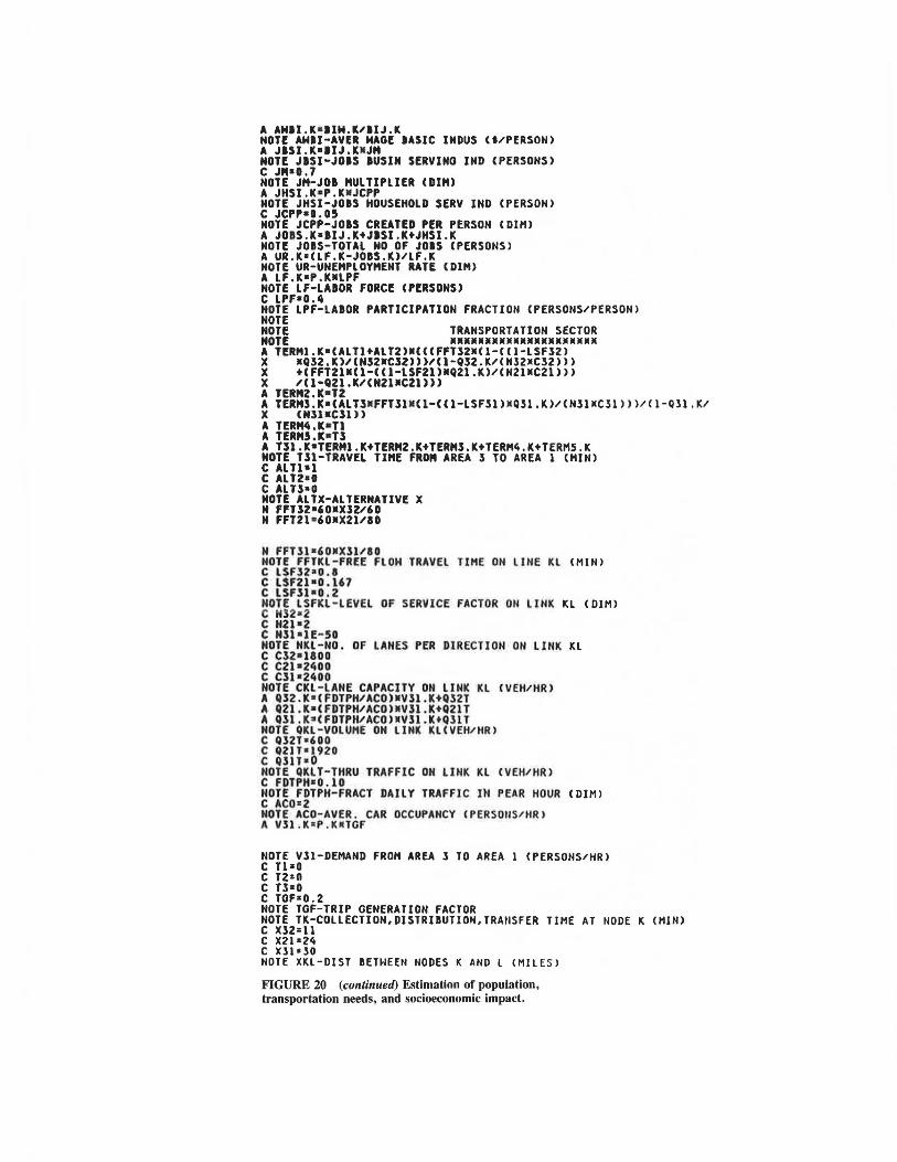
A ANIJ.K•IJN.K,llJ.K NOTE AMII-AVER MAGE IASIC INDUS <t,PERSON> A JISI.K•llJ.K•JM NOTE JISI-JOIS IUSIH SERVINO IND <PERSONS> C JM•0.7 NOTE JM-JOI MULTIPLIER <DIM> A JHSl.K•P.K•JCPP NOTE JHSI-JOIS HOUSEHOLD SERV IND <PERSON> C JCPP•0.05 NOTE JCPP-JOIS CREATED PER PERSON <DIH> A JOIS.K•IIJ.K+JISl.K+JHSI.K NOTE JOBS-TOTAL NO OF JOBS <PERSONS> A UR.K•CLF.K-JOIS.K>,LF.K NOTE UR-UNEMPLOYMENT RATE <DIM> A LF.K•P.K•LPF NOTE LF-LAIOR FORCE <PERSONS> C LPF•0.4 NOTE LPF-LAIOR PARTICIPATION FRACTION <PERSONS/PERSON> NOTE NOTE TRANSPORTATION SECTOR NOTE ••••••••••••••••••••• A TERMl.K•CALTl+ALT2>•<<<FFTS2•Cl-CC1-LSFS2> X •QS2.K>,CNS2•CS2>>>,<1-QS2.K,CN32•Cl2>>> X +CFFT2l•Cl-CC1-LSF21J•Q21.K>,CN21•C21>>> X 'Cl-Q21.K,CN21•C21>>> A TERM2.K•T2 A TERM.S.K•CALTS•FFT.Sl•Cl-CCl-LSFSl>•Qll.K>/(NSl•Cll>>>/Cl-Qll.K/ X <H.SIKC.SU > A TERM4.K•Tl A TERM5.K•T3 A T.Sl.K•TERM1.K+TERM2.K+TERM.S.K+TERM4.K+TERH5.K NOTE Tll-TRAVEL TI"E FRON AREA S TO AREA l CHIN> C ALTl•l C ALT2•0 (; ALT3•0 NOTE ALTX-ALTERNATIVE X N FFTl2•60•Xl2/60 N FFT21 •60•X21/IO

N FFTS1•60•X.Sl/80 NOTE FFTKL-FREE FLOH TRAVEL TIHE ON LINE Kl <MIN> C LSF32•0.8 C LSFZl•O .167 C LSFSl•0.2 NOTE LSFKl-LEVEl OF SERVICE FACTOR ON LINK KL <DIM> C Nl2 11 2 C H21•2 C H3l•lE-50 NOTE NKL-NO. OF LANES PER DIRECTION ON LINK KL C C32•1800 C C21•2400 C Cll•2400 NOTE CKL-LANE CAPACITY ON LINK Kl CVEH/HR> A QS2.K•CFDTPH/ACO>•VS1.K+Ql2T A Q21.K•CFDTPH/ACO>•VS1.K+Q21T A Qll.K•CFDTPH/ACO>•V.Sl.K+QSIT NOTE QKL-VOLUME ON LINK KLCVfH/HR> C Ql2T•600 c Q21T•l920 C Q.SlT•O NOTE QKLT-THRU TRAFFIC ON LINK Kl CVfH/HR> C FDTPH•0.10 NOTE FDTPH-FRACT DAILY TRAFFIC IN PEAR HOUR CDIH> C AC0•2 NOTE ACO-AVER. CAR OCCUPANCY IPERSOttS/HRl I\ Vll .K~P.KllTGF

NOTE V.Sl-DEHAND FROM AREA S TO AREA 1 <PERSONS/HR> c T1:10 c T2•0 C Tl=O C TOF•0.2 NOTE TGF-TRIP GENERATION FACTOR NOTE TK-COLLECTJON,DISTRIIUTIOH,TRAttSFER TIME AT ttODE K CHIN> C X.S2•11 C X21•24 C Xll•lO NOTE XKL-DIST BETHEEN NODES K AND l CHILES)

FIGURE 20 (continued) Estimation of population, transportation needs, and socioeconomic impact.

Drew 81

TABLE 3 TRANSPORTATION DEVELOPMENT EVALUATION METHODOLOGY RESULTS

U5EIZ BENEFIT ANALYSIS

ALTEIZ. E c BC .

1s 1;0000 "1200000 1i;oooooo 2.~e

l34-?7 ooo 18000000 -zr;oooo ooo :z.:z.2

In the mathematical model, parameter values have been cho­sen that support transport improvement to reduce unemploy­ment (see Figure 20). Obviously, the modeling of transportation­induced development in the real world is serious business. The advantage of the system dynamics approach is the absence of the restrictions inherent in the many methodologies. Thus, the dichotomy that exists in a strategy of transport move­ment becomes explicit and must not be obscured by modeling limitations.

REFERENCES

1. D. Drew. System Dynamics: Modeling and Applications. Virginia Polytechnic Institute and State University, Blacksburg, Va., 1986.

2. D. Drew. National Reconstruction and Development Model of Lebanon. American University of Beirut, Beirut, Lebanon, 1981.

NONU5EIZ r.>ENEFIT ANALY'515 (l•Z'5)

10=1000 1'14-000

I.IC) •10 11

1.r;q. 10"' 101000 1';5' 000

UIZ s LI\- JO~~c: "100 WHE.tZE LF. = I".~ LPF t LF., • •

JOB54:• ~1J4'.+Jl)5It+Ji.15J~

IO"I. Oi'.

13JJ4'. = ~ICt/CLIZ; Jl35l*= ~IJ.,•JM ;Jl-151.,· ft· JC PP ('ff FIG :30) IT CAN AL'O Be 5~0Wt-J TI-IAT

P.c Pc Al.JD I +-l !!__I) el lt.1N +- NGF-OMN) t'

ro BIC~· i;1ce-(131Ce-eJc..i)e-t/ALC Wi.!EtZE

P. ,. l l'l"D )U-0~11-1-NGrllLr!Zi.t Thl31) e LfJ) !MN T31f.

TIIE.

~I Cc. ALC• FI Pl<( BlCN )(I- FIOIN·e(l-nrn)t C0~1.J

3. D. Drew and T. Tran. Land Use Dynamics: A Comparison of the Lowry and Forrester Models. Proc., 8th Annual Conference on Modeling and Simulation, University of Pittsburgh, Pa., 1978.

4. D. Drew. Methodologies for Transportation-Economic Devel­opment. Presented at 68th Annual Meeting of the Transportation Research Board, Washington, D.C., January 22-26, 1989.

5. D. Drew and C. Hsieh. A Systems View of Development: Meth­odology of Systems Engineering and Management. Cheng Yang Publishing Co., Taipei, Taiwan, 1984.

6. D. Drew. The Growth Shapers: Infrastructure Induced Devel­opment. In Systems Models for Decision Making Chapter 5, N. Sharij and P. Adulbhan, eds., Asian Institute of Technology, Bangkok, Thailand, May 1978.

7. D. Drew. Bicol River Basin Development Program Simulation Model. USAID/Philippines Project No. 492-51-190-126, Manila, Philippines, 1975.

8. J. Forrester. Urban Dynamics. The M.I.T. Press, Massachusetts Institute of Technology, Cambridge, 1969.

9. J. Forrester. Principles of Systems. Wright-Allen Press, Inc., Cambridge, Mass., 1968.