Synthetic Storm Modeling for Millimeter Wave Band Mesh Networks

Synthetic Storm Modeling forMillimeter Wave Band Mesh Networks

Bharatwajan Raman

B.E., Electronics and Communication Engineering,Anna University, India, 2005

Submitted to the Department of Electrical Engineering andComputer Science and the Faculty of the Graduate School

of the University of Kansas in partial fulfillment ofthe requirements for the degree of Master of Science

Thesis Committee:

Dr. James P.G. Sterbenz: Chair

Dr. Alexander M. Wyglinski: Co-Chair

Dr. Victor S. Frost

Date Defended

c© 2008 Bharatwajan Raman

2008/06/11

The thesis committee for Bharatwajan Raman certifies

that this is the approved version of the following thesis:

Synthetic Storm Modeling for Millimeter Wave Band Mesh Networks

Committee:

Chair

Co-Chair

Date Approved

i

Abstract

In this thesis, a novel method of modeling the characteristics of a storm and

its effects on a millimeter wave band (70 – 90 GHz) mesh network is presented.

A storm system is generated using synthetic data; the movement of the system

through a network is simulated and attenuation on individual links is calculated

using existing models relating rain rate and attenuation. Finally, the collective

effect of attenuated links on network performance is analyzed. This model is

particularly useful in implementing predictive routing algorithms, as knowledge

of weather phenomenon is usually available several minutes in advance, which has

the potential to improve or eliminate losses due to routing reconvergence.

ii

Contents

Acceptance Page i

Abstract ii

List of Figures vi

List of Tables vii

1 Introduction 1

1.1 Weather Disruption in the Real World . . . . . . . . . . . . . . . 3

1.2 Research Contributions . . . . . . . . . . . . . . . . . . . . . . . . 4

1.2.1 Synthetic Storm Modeling . . . . . . . . . . . . . . . . . . 4

1.2.2 Simulation Model . . . . . . . . . . . . . . . . . . . . . . . 5

1.2.3 Link Modeling . . . . . . . . . . . . . . . . . . . . . . . . . 7

1.3 Thesis Organization . . . . . . . . . . . . . . . . . . . . . . . . . . 7

2 Background and Related Work 8

2.1 Background . . . . . . . . . . . . . . . . . . . . . . . . . . . . . . 8

2.1.1 Millimeter Wave Transmission Systems . . . . . . . . . . . 9

2.1.2 Losses in MWB Propagation . . . . . . . . . . . . . . . . . 13

2.2 Related Work . . . . . . . . . . . . . . . . . . . . . . . . . . . . . 20

2.2.1 Modeling Attenuation due to Rain . . . . . . . . . . . . . 20

2.2.2 Link Modeling . . . . . . . . . . . . . . . . . . . . . . . . . 24

2.2.3 Storm Modeling . . . . . . . . . . . . . . . . . . . . . . . . 25

3 Synthetic Storm Modeling 27

3.1 Geometric Modeling . . . . . . . . . . . . . . . . . . . . . . . . . 28

iii

3.1.1 Storm Geometry . . . . . . . . . . . . . . . . . . . . . . . 28

3.1.2 Storm Movement . . . . . . . . . . . . . . . . . . . . . . . 31

3.2 Link Attenuation . . . . . . . . . . . . . . . . . . . . . . . . . . . 32

3.2.1 Calculation of Fraction of Links Affected . . . . . . . . . . 33

3.2.2 Attenuation on Affected Links . . . . . . . . . . . . . . . . 37

4 Mesh Network Simulation 41

4.1 Simulation Model . . . . . . . . . . . . . . . . . . . . . . . . . . . 41

4.1.1 Storm Structure . . . . . . . . . . . . . . . . . . . . . . . . 42

4.1.2 Storm Patterns . . . . . . . . . . . . . . . . . . . . . . . . 42

4.2 Network Simulation and Parameters . . . . . . . . . . . . . . . . . 42

4.2.1 Network Topology and Characteristics . . . . . . . . . . . 43

4.2.2 Traffic . . . . . . . . . . . . . . . . . . . . . . . . . . . . . 43

4.2.3 Performance Evaluation . . . . . . . . . . . . . . . . . . . 44

4.3 Results and Analysis . . . . . . . . . . . . . . . . . . . . . . . . . 44

4.3.1 Case 1: Vertical Storm Pattern . . . . . . . . . . . . . . . 44

4.3.2 Case 2: Diagonal Storm Pattern . . . . . . . . . . . . . . . 48

4.3.3 Case 3: Diagonal Pattern with Larger Storm . . . . . . . . 50

5 Link Modeling 55

5.1 Markov Process . . . . . . . . . . . . . . . . . . . . . . . . . . . . 56

5.2 Measurement Setup . . . . . . . . . . . . . . . . . . . . . . . . . . 57

5.3 Three-State Markov Model . . . . . . . . . . . . . . . . . . . . . . 59

6 Conclusions and Future Work 65

6.1 Conclusions . . . . . . . . . . . . . . . . . . . . . . . . . . . . . . 66

6.2 Future Work . . . . . . . . . . . . . . . . . . . . . . . . . . . . . . 67

A ITU-R P.838-3 Coefficients 70

References 72

iv

List of Figures

1.1 Absorption by atmospheric elements [1, 2] . . . . . . . . . . . . . . 2

1.2 Absorption by atmospheric elements [2] . . . . . . . . . . . . . . . 3

1.3 Obtaining FER on each link from the storm model . . . . . . . . 6

2.1 Free space path loss vs. distance . . . . . . . . . . . . . . . . . . . 13

2.2 Gaseous absorption curves [2, 3] . . . . . . . . . . . . . . . . . . . 15

2.3 Frequency vs. attenuation . . . . . . . . . . . . . . . . . . . . . . 18

2.4 Rain rate vs. attenuation . . . . . . . . . . . . . . . . . . . . . . . 19

2.5 Crane rain zones in the US [2] . . . . . . . . . . . . . . . . . . . . 21

3.1 Elliptical modeling of storm . . . . . . . . . . . . . . . . . . . . . 29

3.2 Radar image with light and heavy rain zones . . . . . . . . . . . . 30

3.3 Elliptical modeling of radar images . . . . . . . . . . . . . . . . . 31

3.4 Storm movement generated in an 8×8 mesh . . . . . . . . . . . . 32

3.5 Storm movement in an arbitrary mesh with 6 nodes . . . . . . . . 33

3.6 Link entirely encompassed by the cell . . . . . . . . . . . . . . . . 35

3.7 Fraction of the link affected by the cell . . . . . . . . . . . . . . . 36

3.8 Link covered at one end by the cell . . . . . . . . . . . . . . . . . 36

3.9 FER vs. rain rate for a 1 mile link at 73.5 GHz . . . . . . . . . . 39

3.10 FER vs. rain rate for a 5 mile link at 73.5 GHz . . . . . . . . . . 40

4.1 Case 1: Topology of the mesh used in simulations . . . . . . . . . 43

4.2 Case 1: Storm moves along the edge of a network . . . . . . . . . 45

4.3 Case 1: Packets lost across affected links . . . . . . . . . . . . . . 46

4.4 Case 1: Throughput of all received bits . . . . . . . . . . . . . . . 48

4.5 Case 1: Throughput of all dropped bits . . . . . . . . . . . . . . . 48

4.6 Case 2: Storm moves diagonally across the network . . . . . . . . 49

v

4.7 Case 2: Throughput of all received bits . . . . . . . . . . . . . . 51

4.8 Case 2: Throughput of all dropped bits . . . . . . . . . . . . . . 51

4.9 Case 3: Storm moves diagonally across the network . . . . . . . . 52

4.10 Case 3: Throughput of all received bits . . . . . . . . . . . . . . 54

4.11 Case 3: Throughput of all dropped bits . . . . . . . . . . . . . . 54

5.1 MWB test topology . . . . . . . . . . . . . . . . . . . . . . . . . . 57

5.2 Three-state Markov model of link states . . . . . . . . . . . . . . 59

5.3 Quantization of link performance to three levels . . . . . . . . . . 60

6.1 Measured FER vs. FER derived from ITU-R P. 838-3 . . . . . . . 68

vi

List of Tables

2.1 Beamwidth at 1 km with 30 cm diameter antennas . . . . . . . . 10

2.2 Fresnel zone clearance . . . . . . . . . . . . . . . . . . . . . . . . 11

2.3 Attenuation at 99.99% availability for a 3 km link [4] . . . . . . . 23

4.1 Case 1: Simulation information . . . . . . . . . . . . . . . . . . . 47



5.1 24-hour state probabilities without FEC (Jun. 2007) . . . . . . . 61

5.2 24-hour TPM without FEC (Jun. 2007) . . . . . . . . . . . . . . 61

5.3 State probabilities with FEC (Jul. 2007–Feb. 2008) . . . . . . . . 61

5.4 TPM with FEC (Jul. 2007–Feb. 2008) . . . . . . . . . . . . . . . 62

5.5 State probabilities without FEC (Jul. 2007–Feb. 2008) . . . . . . 62

5.6 TPM without FEC (Jul. 2007 – Feb. 2008) . . . . . . . . . . . . 62

A.1 Coefficients for kH . . . . . . . . . . . . . . . . . . . . . . . . . . 70

A.2 Coefficients for kV . . . . . . . . . . . . . . . . . . . . . . . . . . . 70

A.3 Coefficients for αH . . . . . . . . . . . . . . . . . . . . . . . . . . 71

A.4 Coefficients for αV . . . . . . . . . . . . . . . . . . . . . . . . . . 71

vii

Chapter 1

Introduction

The advent of video sharing sites, IPTV (internet protocol television), mobile

video applications, and ubiquitous, highly affordable devices has ushered in an

era of millions of people using voice and data networks, fixed and mobile for new

applications. This trend is not likely to slow in the near future, and requires

increasing bandwidth. Optical fibers provide the necessary bandwidth, but, not

all carriers have access to affordable use of cables, and expansion is frequently

impractical because of issues such as deployment costs [5, 6] and governmental

regulations. In the wireless domain, the spectrum that is used by current tech-

nologies has been allocated by the Federal Communications Commission (FCC)

in the US, but none of these technologies provide bandwidth comparable to that

of optical fibers. The unlicensed 60 GHz band has been in use for some time now,

but suffers range limitations due to oxygen absorption and weather-related atten-

uation. The free space optical band (FSO) can support higher bandwidths but is

heavily attenuated by fog, smog, and other atmospheric impairments. Figures 1.1

and 1.2 show absorption due to atmospheric elements.

A lot of interest has been shown in the spectrum ranging from 70–95 GHz,

1

Figure 1.1. Absorption by atmospheric elements [1, 2]

referred to as millimeter wave band (MWB) after the FCC opened it for licensing.

The MWB is particularly attractive for a variety of reasons such as high band-

width, low interference, efficient frequency reuse, and light license regulations.

But, the paramount consideration in drafting link budgets at these frequencies

is attenuation due to hydrometeors (rain, snow, hail, dew). There have been

empirical models developed based on samples of rain measurements throughout

the world that provide reasonable values of long-term fade probabilities, but they

are highly specific to the area in which measurements were made and not useful

to represent short-term channel conditions.

2

Figure 1.2. Absorption by atmospheric elements [2]

1.1 Weather Disruption in the Real World

In the real world, an assortment of atmospheric factors is responsible for signal

degradation in MWB links with rain playing a major role. Higher values of rain

rate result in greater attenuation.

For determining the performance of MWB mesh networks, it is important to

understand the dynamics of weather phenomena and their effects on the links.

This is not a straightforward task because the attenuation on a link is due to the

collective effect of various factors such as rainfall rate, drop size, wind velocity, and

polarization of the rain drops. Therefore, it is not easy to build an analytical model

to capture weather effects on MWB transmissions. Furthermore, weather events

are local in scope and bursty in nature; therefore deriving a generic analytical

3

expression to measure spatial correlation of rain attenuation is impractical. An

impairment model is a more practical approach. While an empirical link model

at best can capture rain attenuation along a single link, a simulation model is

necessary to understand the effects of the weather event on the mesh network as

a whole. This work proposes a technique to model effects of a storm system on a

mesh network.

1.2 Research Contributions

The following are the major contributions of this thesis work:

• Develop a synthetic storm model with structure and trajectory which rep-

resents the characteristics of a real-world storm and model the effects of the

storm on a millimeter wave mesh network.

• Simulate the effects of rain attenuation on network performance using the

network simulator ns-2 [7].

• Formulate long-term statistics of rain attenuation using a three-state Markov

model. The model is built from actual measurements of frame error rates

on a physical link.

The following subsections introduce these contributions in more detail.

1.2.1 Synthetic Storm Modeling

A major portion of this work deals with modeling a storm system with multiple

rain cells, simulating its movement through a mesh network, and calculating the

attenuation on the links affected by the storm system passing above. The process

4

flow is detailed in Figure 1.3. This model can help simulate rain events and

calculate attenuation due to rain on each link at every instant. If fed with real

storm data, it can be used in real time to calculate and predict the attenuation

on each link and hence will aid in developing predictive routing strategies to route

around links affected by rain. The methodology is discussed in detail in Chapter 3.

1.2.2 Simulation Model

The effect of rain events on overall network performance is simulated using

the ns-2 simulation package. A mesh-network model is built, CBR (constant

bit rate) traffic is exchanged between arbitrary nodes, and loss on each link is

modified according to the movement of the storm. Performance parameters such

as throughput, delay, and number of packets dropped are monitored to evalu-

ate mesh-network performance. The details of the simulation are discussed in

Chapter 4.

5

synthetic storm model(system of ellipses)

effective attenuation in dB(i,j) = i×dj

bit error rateBER = f ((Eb/N0)rain_event)

frame error rateFER = 1− (1− BER)n

synthetic storm data( ai , bi, θi, hi, ki, v, Ri )

attenuation in dB/km (ITU-R)i = f(Ri)

fraction of link affected by the storm (dj) in km

received signal to noise ratio (per bit)(Eb/N0)rain_event = (Eb/N0)clear_sky − Γ(i,j)

network throughput and efficiency analysis

Figure 1.3. Obtaining FER on each link from the storm model

6

1.2.3 Link Modeling

A method to calculate long-term and short-term statistics of rain attenuation

is also developed in this thesis. A Markov model representing strength of con-

nectivity is constructed with three states: strong, weak, and disconnected. The

model’s state and state-transition probability values are obtained from measure-

ments on a real link operating at 73.5 Ghz within the millimeter wave band. With

this model, depending on the number of samples, we can obtain daily, monthly

or yearly rain attenuation statistics. A useful quantity is worst-month statistics

used by network planners to determine antenna gains on millimeter wave radios.

The formulation of the model is explained in detail in Chapter 5.

1.3 Thesis Organization

The rest of the thesis is organized as follows: Chapter 2 discusses the prop-

erties of MWB signals and their propagation characteristics, losses suffered at

MWB frequencies due to gaseous absorption, foliage, scattering and diffraction,

and research work published in literature pertaining to rain attenuation model-

ing, link modeling, and storm modeling. Chapters 3, 4, and 5 detail the major

contributions of this thesis. In Chapter 3, modeling of synthetic storms is pre-

sented. In Chapter 4, modeling of link behavior using a three-state Markov model

is presented. In Chapter 5, mesh-network performance evaluation using ns-2 sim-

ulations is discussed. Chapter 6 outlines the conclusions arrived at from this

research and future work that will improve this thesis and expand its scope.

7

Chapter 2

Background and Related Work

This chapter contains a background study on millimeter wave transmissions

and a discussion of realted work in the areas of rain attenuation modeling, storm

modeling, and link modeling.

This chapter is organized as follows: First, a background section details the

properties of MWB (millimeter wave band) systems such as frequency bands,

beamwidth, antenna, power requirements, and power spectral density and propa-

gation characteristics such as losses and fading. Then, related work is presented

that discusses works in literature that deal with rain attenuation and modeling

storm systems.

2.1 Background

MWB communication technology is fairly new with the FCC inviting licensing

bids as recently as 2003 in the US. Service rules for MWB were first specified

in 2003 [8] and later modified in 2004 and 2005 [9]. This section details the

characteristics of the MWB as well as losses in MWB links.

8

2.1.1 Millimeter Wave Transmission Systems

Transmission characteristics such as frequency range, beamwidth, antenna,

power requirements, and power spectral density limits are discussed in this section.

Knowledge of transmission characteristics is useful in designing nodes that are part

of the mesh network used to simulate the effects of rain on network performance.

2.1.1.1 Frequency Band and Assignments

The range of frequencies between 30 GHz and 300 GHz have wavelengths on

the order of millimeters. The MWB licensed by the FCC in the US consists of

frequencies in the bands 71–76 GHz, 81–86 GHz and 92–95 GHz. The 92–95

GHz band is further divided into three segments: 92.0–94.0 GHz and 94.1–95.0

GHz for government and non government users and 94.0–94.1 GHz for US Federal

Government use. Initially, the 71–76 GHz and 81–86 GHz bands were divided

into four unpaired segments of 1.25 GHz each with a loading requirement of 1

bit/second/hertz (bps/Hz) with no aggregation limits. This was modified later

to no segmentation and a loading requirement of 0.125 bps/Hz for ease of band

reallocation and use of simple, inexpensive modulation schemes like on-off keying

(OOK) or binary phase shift keying (BPSK) [9].

2.1.1.2 Beamwidth

Beamwidth is defined as the angle between the half-power points on the main

lobe. The half-power, or the 3 dB points are with respect to the peak power of

the main lobe. The beamwidth of a signal determines the density of the nodes

in a network. Links operating with smaller beamwidths allow more spatial reuse

permitting a greater number of nodes to be packed within a given geographi-

9

cal area compared to wider beamwidth links. Millimeter wave signals have very

narrow beamwidth sometimes referred to as pencil beam. Table 2.1 shows the

beamwidths of signals at different frequencies [10].

Table 2.1. Beamwidth at 1 km with 30 cm diameter antennas

Frequency [GHz] Beamwidth [degrees] Beamwidth [meters]

2.4 117◦ 1989

24 12◦ 204

60 4.7◦ 79.9

80 1.2◦ 20.4

It is seen that there is very little chance for interference if there is adequate

seperation between antennas, which is in tens of meters as seen in Table 2.1.

Higher diameter antennas reduce beamwidth, which enables a square mesh of

several nodes with directional antennas in 4 orthogonal directions. Tests have in-

dicated that it is possible to deploy up to 200 non interfering MWB antennas on

the roof of a single skyscraper [9]. Fresnel zone calculations indicate a clearance

of less than 10 meters from any obstruction needed for acceptable signal levels

at the receiver. Fresnel zones are concentric regions in which the path length of

the secondary waves differ by nλ/2 from that of the line of sight (LOS) com-

ponent, where n is the nth Fresnel zone and λ is the wavelength of the signal

in meters [11]. A λ/2 difference in path length will cause a phase shift of 180◦,

thus causing destructive interference between the secondary wave and the LOS

component. So, first Fresnel zone clearance is important to avoid interference.

All components with a path length difference of odd multiples of λ/2 will cause

destructive interference, but as n increases, the intensity of the secondary waves

decreases. Table 2.2 shows a list of first Fresnel zone radii midway for antennas

10

seperated by distance d.

Table 2.2. Fresnel zone clearance

Frequency [GHz] First Fresnel zone [m]

d = 1 km d = 5 km

2.4 5.59 12.5

24 1.77 3.95

60 1.12 2.5

70 1.04 2.31

80 0.97 2.17

The Fresnel zone radius at any point P in the middle of a link is given by:

Fn =

√nλd1d2

d1 + d2

(2.1)

where n is the nth Fresnel zone, Fn is the radius of the nth Fresnel zone in meters,

d1 is the distance of point P from one end of the link in km, d2 is the distance

of point P from the other end of the link in km, and λ is the wavelength of the

signal in meters.

The first Fresnel zone contains the strongest signals. These numbers show that

network planning will be relatively easy even in a dense urban environment. As

beam spreading is minimal, structures and foliage will not cause interference if a

line-of-sight path exists between the transmitter and receiver with a Fresnel first

zone clearance from obstructing structures.

11

2.1.1.3 Antenna and Power Requirements

The FCC specifies a minimum antenna gain of 43 dBi (forward gain of the

antenna compared to an isotropic antenna) and a half-power beamwidth of 1.2◦

for MWB links. Initial technical requirements specified a gain of 50 dBi and 0.6◦

half-power beamwidth. While larger beamwidths result in interference between

closely spaced antennas, very small beamwidths have their own share of problems.

A 0.6◦ half-power beamwidth and 50 dBi gain is possible only with two feet an-

tennas which are more expensive than one-foot antennas that have a half-power

beamwidth of 1.2◦. In most places, existing infrastructure is insufficient to de-

ploy bigger antennas; they need stronger towers thereby increasing deployment

costs [9]. Finally, a 0.6◦ beamwidth signal complicates tower siting and often re-

sults in signal loss by the receiver because of tower sway, which is not uncommon

in high-rise buildings. Error-angle fading (Section 2.1.2.5) is also pronounced at

smaller beamwidths. The cost reduction by using smaller antennas enables wider

deployment, thereby bridging the gap to buildings that are a couple of miles away

from a fiber point-of-presence (POP) but that cannot have fiber connections [5,9].

2.1.1.4 Power Spectral Density Limit

Power spectral density (PSD) is a measure of how power is distributed across

the frequencies in a particular frequency range. For example, given a range of 5

GHz and a transmit power limit of 7.5 W, it is possible to transmit the power

using all of the 5 GHz bandwidth or only a portion of it, say, 100 MHz. The

spectral properties of these two signals would be radically different. One of the

main deployment advantages of MWB links is frequency reusability. This is made

possible by the short range of wideband links. If no limit is imposed on power

12

spectral density, narrowband links can be used that will have a much longer range,

thereby causing interference and reducing frequency reuse. Therefore, a PSD limit

of 150 mW/100 MHz is enforced to make efficient use of the spectrum.

2.1.2 Losses in MWB Propagation

This section discusses losses due to various factors in MWB links. These

losses consist of free space path loss, attenuation due to atmospheric gases, foliage

loss, scattering and refractive effects in particulate matter, refractive effects and

scintillation.

2.1.2.1 Free Space Path Loss

1 2 3 4 5 6 7 8 9 10 11 12 13 14 15120

130

140

150

160

170

180

190

Distance [km]

Free

spa

ce p

ath

loss

[dB

]

60 GHz70 GHz80 GHz90 GHz

Figure 2.1. Free space path loss vs. distance

Free space path loss is the reduction in received signal strength with distance.

13

It is dependent on the frequency of the signal and the distance between the trans-

mitting and receiving antennas.

In clear-sky conditions, free space path loss is given by [2]:

LFSL = (4πR/λ)n (2.2)

where, LFSL is the free space path loss, R is the distance between transmit and

receive antennas in km, λ is the operating wavelength in meters, and n is the path

loss exponent. The path loss exponent is 2 in most cases.

Substituting n = 2 and rewriting in terms of frequency [f ],

LFSL [dB] = 92.4 + 20 log f + 20 logR (2.3)

Thus, the higher the frequency, the higher the path loss, for example, 129.5 dB for

71 GHz at 1 km and 131.2 GHz for 86 GHz at 1 km. Figure 2.1 shows free space

path loss vs. distance for various millimeter wave frequencies, obtained from

Equation 2.3. Given the fact that there are PSD limits and heavy path losses

over larger distances, it is not possible to have very long millimeter wave links,

and rain attenuation will further decrease the range of MWB links if availability

requirements have to be met. Rain attenuation is discussed in Subsection 2.1.2.6.

2.1.2.2 Attenuation due to Atmospheric Gases

The major contributors to gaseous attenuation in MWB signals are oxygen and

water vapor. Molecular interactions cause attenuation due to scattering and are

appreciably higher near the frequency of resonance of the molecules. Attenuation

14

Figure 2.2. Gaseous absorption curves [2, 3]

due to oxygen at ground level and a temperature of 15◦ is given by [12]:

αO[dB/km] =

[3.79× 10−7f +

0.265

(f − 63)2 + 1.59+

0.028

(f − 118)2 + 1.47

](f+198)2×10−3

(2.4)

for f > 63 GHz where f is the frequency of the signal.

Attenuation due to water vapor at sea level and at a temperature of 15◦ for f < 350

GHz and ρ < 12 g/m3 where ρ is the water vapor density given by [12]:

αw[dB/km] =

[0.050 + 0.0021ρ+

3.6

(f − 22.2)2 + 8.5+

10.6

(f − 183.3)2 + 9

+8.9

(f − 325.4)2 + 26.3

]f 2ρ× 10−4 (2.5)

15

Note that these formulae are applicable at ground level within a pressure range of

1013 ± 50 mbar, at a temperature of 15◦C. Other temperatures may be taken into

account by correction factors of −1%◦C−1 from 15◦C for dry air, and −0.6%◦C−1

from 15◦C for water vapor, valid over the range from −20◦C to +40◦C. [13]

Figure 2.2 shows the losses due to oxygen and water vapor absorption. These

plots were obtained from Equations 2.4 and 2.5, which are empirical formulae

obtained from measurements.

2.1.2.3 Foliage Loss

The loss caused by vegetative obstructions is called foliage loss and it causes

significant attenuation in millimeter wave frequencies. If there is foliage near the

first Fresnel zone, multipath effects degrade the signal to a great extent. For a

depth of less than 400 meters, the loss (L) is given by [2]:

L = 0.2f 0.3R0.6 (2.6)

where f is the frequency in MHz and R is the depth of foliage in meters (R <400).

The above relationship is applicable for frequencies ranging between 0.2 GHz and

95 GHz.

2.1.2.4 Scattering and Absorption in Particulate Matter

Particulate matter such as sand and dust particles have sizes comparable to the

wavelengths of millimeter wave signals. Hence, scattering is common when there

is a lot of dust in the air. Other key properties apart from size that govern the

extent of attenuation are shape, density, and dielectric properties of the particles.

16

The propagation constant a, is [14]

a = α + jβ (2.7)

where,

α = 3.431× 106fNr3 ε′′

(ε′ + 2)2 + ε′′2

β = 7.545× 106fNr3 (ε′ − 1)(ε′ + 2) + ε′′2

(ε′ + 2)2 + ε′′2

where, f is the frequency of the signal, N is the number of dust particles in unit

volume, r is the radius of the dust particle, ε′ and ε′′ are dielectric constants

measured from saline dust storms. A detailed discussion on particulate scattering

is found in [14] and [13].

2.1.2.5 Refractive Effects and Scintillation

Temperature and pressure variations result in different advective (horizontal)

and convective (vertical) velocities of various layers in the atmosphere. This results

in inhomegeneity of the atmosphere and thus, different sections of the atmosphere

have different refractive indices. Two important phenomena that arise out of

refractive effects are multipath fading and error-angle fading.

Multipath fading occurs when the receiver receives multiple copies of the same

signal, each delayed by a different amount. This phenomenon is not significant in

short path lengths, but should be accounted for when path lengths exceed three

km [15]. As the signal travels from one point to another, the spread beam passes

through various layers of the atmosphere with different refractive indices. When

the distance is greater, the beam-spreading is greater and the number of layers

17

traversed by the signal components becomes greater. Therefore, multipath effects

are greater at longer lengths.

Error-angle fading, or beam-whipping, happens when the displacement of the

beam from the center of the receiving antenna becomes so large that the receiver

completely misses the signal.

Scintillation is defined as the short-term variations of refractive index associ-

ated with air turbulence. A prediction method for calculating statistical properties

of signal fluctuations due to scintillation is presented in [16].

2.1.2.6 Rain Attenuation

Figure 2.3. Frequency vs. attenuation

Rain fading is the most dominant of all the factors contributing to atmo-

spheric attenuation. This is because the size of rain drops is comparable to the

18

wavelengths of MWB signals, which causes scattering of the signal. Attenuation

due to rain is dependent on the size of rain drops, rain rate, velocity, and polar-

ization of rain drops. Of these, rain rate is the principal factor that decides the

extent of attenuation. Very light rain affects link performance marginally, while

heavy rains can completely degrade link performance. Figure 2.3 shows the at-

tenuation due to rain at various millimeter wave frequencies, obtained using the

ITU-R P.838-3 curves (explained in Section 2.2.1.2). Figure 2.4 shows the atten-

uation due to rain in MWB. Link planners use measurements of rain rate in a

particular region and plots such as the one shown in Figure 2.3 to predict outages

due to rain. Attenuation data are not as readily available as rainfall data. So,

a relationship like this will be useful for predicting attenuation given the rainfall

statistics of a region. Empirical formulae have been developed based on measure-

0 10 20 30 40 50 60 70 80 90 1000

5

10

15

20

25

30

35

Rain rate [mm/h]

Atte

nuat

ion

[dB

/km

]

90 GHz

80 GHz

70 GHz

60 GHz

Figure 2.4. Rain rate vs. attenuation

19

ments of rainfall and attenuation. Two such models are the Crane model and the

ITU-R P. 838-3 model. These are explained in detail in the following sections.

2.2 Related Work

This section discusses work done in modeling rain attenuation, storm modeling,

and link modeling at millimeter wave frequencies.

2.2.1 Modeling Attenuation due to Rain

This section deals with the measurement of attenuation due to rain, channel

modeling in millimeter wave frequencies and network planning considerations in

literature.

The effects of rain on MWB transmissions have been studied for decades with

results published relating attenuation and rain rate. There are two approaches to

modeling attenuation due to rain: developing analytical models based on phys-

ical phenomena and building empirical models based on measurements. Due to

multiple atmospheric factors contributing to attenuation, it is difficult to develop

an analytical model based on the physics of the phenomena. On the other hand,

empirical models are more practical to develop and are reasonably accurate in

predicting the long-term effects of rain and other atmospheric phenomena on mil-

limeter wave transmissions [17], [18] and [4]. Two models widely used in designing

millimeter wave systems are the Crane model and the ITU-R P.838-3 model. Both

the models use“rain-zones”, or areas in which long term statistics of rain are cor-

related. Each zone corresponds to a standard set of coefficients that are used in

calculating attenuation due to rain. Figure 2.5 shows the Crane zones in the US.

These two methods are next discussed briefly, followed by millimeter wave

20

Figure 2.5. Crane rain zones in the US [2]

channel modeling research and storm modeling studies.

2.2.1.1 Crane Model

Robert. K. Crane developed the global (Crane) model for rain attenuation in

1980. It was based “entirely on geophysical observations of rain rate, rain struc-

ture, and the vertical variation of atmospheric temperature” [19]. Attenuation is

calculated from rain rates using [20]:

A(Rp, D) = αRβp

[euβd − 1

uβ− bβecβd

cβ+bβecβD

cβ

],

d 6 D 6 22.5 km

(2.8)

21

A(Rp, D) = αRβp

[euβD − 1

uβ

], 0 < D 6 d (2.9)

where A is the signal attenuation in dB, D is the rain affected path length, Rp is

the rain rate in mm/h, α, and β are numerical constants, and u, b, c, and d are

empirical constants defined as:

u =ln(becd)

d

b = 2.3R−0.17p

c = 0.026− 0.03 lnRp

d = 3.8− 0.6 lnRp.

In 1982, Crane proposed the two-component rain attenuation model based on “the

observations of volume cells and debris and an ad hoc procedure to account for

the spatial correlations for each component” [19]. It was revised in 1989 and is

called the revised Crane two-component model.

2.2.1.2 ITU-R P.838-3

The International Telecommunication Union (ITU) outlines a procedure to

calculate attenuation from rain rates in ITU-R P.838-3. According to the recom-

mendation, attenuation is given by [21]:

γR = kRα (2.10)

where γR is the attenuation in dB/km, R is the rain rate in mm/h, and k and

α are obtained from the following equations:

22

log 10k =4∑j=1

ajexp

[−(

log 10f − bjcj

)2]

+mk log 10f + ck (2.11)

α =5∑j=1

ajexp

[−(

log 10f − bjcj

)2]

+mα log 10f + cα (2.12)

where f is the frequency in GHz, k is either kH or kV , α is either αH or αV .

kH and αH are constants for horizontal polarization and kV and αV are constants

for vertical polarization. For linear and circular polariation, k and α are obtained

from the following equations:

k = [kH + kV + (kH − kV )cos2θcos2τ ]/2 (2.13)

and

α = [kHαH + kV αV + (kHαH − kV αV )cos2θcos2τ ]/2k (2.14)

where θ is the path elevation angle (θ = 0 for terrestrial paths) and τ is the

polarization tilt angle relative to the horizontal. Equations 2.11 and 2.12 were

developed from “curve-fitting to power-law coefficients derived from scattering

calculations” [21]. Table 2.3 compares the ITU and Crane models [4].

Table 2.3. Attenuation at 99.99% availability for a 3 km link [4]

ITU Zone/Crane Zone Units E/F D/C K/D2 N/E

Rain rate ITU/Crane mm/hr 22/22 19/29 42/47 95/91

ITU-R 530 dB 10.8 14.3 22.3 39.2

Crane global dB 13.2 17.2 25.7 45.9

Crane 2-component(TC) dB 13.6 18.4 28.8 52.0

Crane revised TC dB 12.4 20.0 26.9 51.3

23

It is seen from Table 2.3 that the Crane models are a little pessimistic relative

to the ITU model in that they suggest higher attenuation for the same value of

rain rate. The ITU model is used in this work for calculating attenuation due to

rain, since it is an international standard. Furthermore, manufacturers of MWB

equipment use the ITU model to design their links [22] .

2.2.2 Link Modeling

In this section, background that deals with link modeling in the millimeter

wave range and modeling of storm structures is presented.

A number of models have been described in literature about modeling links

affected by rain. These are either variants of the Crane/ITU model, or Markov

models built from measurement of rain and attenuation over time, or a combina-

tion of both.

Hendrantoro et al. [23] propose a multivariate autoregressive model for rain

attenuation and simulate it on two short links operating at 30 GHz. An autoregres-

sive model of rain attenuation is built using spatial and temporal measurements

of rainfall and attenuation. This model can be used to simulate rain events on a

network with short links that show significant correlation in the rain rates they

see. The spatio-temporal characteristics of rainfall must be known at both sites.

This model is highly location specific like most others.

Dissanayake et al. [24] discuss a method to quantify the combined effect of

various atmospheric phenomena on Ka-band links. Rain attenuation, cloud at-

tenuation, gaseous absorption, melting layer attenuation, and refractive effects are

combined to give a single value of attenuation.

Utsunomiya and Sekine [25] discuss attenuation at millimeter and sub millime-

24

ter wavelengths. They compare attenuation due to rain using several drop size

distributions and declare that a Weibull distribution yields best results.

Alasseur et al. [26] discuss a couple of methods to model rain-rate time-series

for attenuation calculations. Both methods employ heirarchical Markov chains:

the outer chain deciding if there is rain or not (duration of rain events) and the

inner chain deciding the intensity of the rain if present.

2.2.3 Storm Modeling

Montopoli et al. [27] characterize the shape of rain storms using C-band radar

data. They model horizontal profiles of rain cells using three analytical models

and measurements from radar.

Fontan et. al. [28] propose a technique to convert rain-rate series to attenuation

series using a synthetic storm technique. They evaluate their technique on an

event-by-event basis using a 40 GHz satellite link. Their model involves simulating

rain events of two types: quasi-flat and spiky. The former is a longer event and

has moderate rainfall associated with it. The latter is short but is associated with

heavy rainfall.

Daru et al. [29] investigate the space and time correlation of rain attenua-

tion based on measurements made using a network that has star topology. They

present measurements taken from links in Hungary and a correlation analysis of

rain attenuation across multiple links within a geographical area. Spatial correla-

tion as a function of angular seperation between the links is plotted. This work

quantifies the space and time correlation of rain attenuation based on measure-

ments, but does not propose techniques to simulate the effects of rain.

Riva [30] reviews state-of-the-art research in the field of spatial distribution of

25

propagation parameters affecting millimeter wave band frequencies. He character-

izes properties of rain cells like shape, peak intensity, dimension, and movement

direction and speed. Rain cells are elliptically modeled and cell diameter distri-

bution of oceanic and land rain cells is presented.

Most of these papers discuss means to obtain time-series values of attenuation

given the rain-rate statistics of a region using a reference model such as the Crane

model or the ITU-R model. Very few discuss the spatial characterization of storms

and how to extract spatial correlation of rain attenuation given the geometry of

the storm. This thesis proposes a method to calculate attenuation due to rain

on links given the structures and positions of storm cells. Though it does not

provide a closed form expression for spatial correlation, the results can be used

to simulate the effects of rain on a mesh network or in dynamic routing schemes

where knowledge of attenuation is required in real time.

26

Chapter 3

Synthetic Storm Modeling

This chapter deals with synthetic storm modeling, which involves character-

izing the properties of a real-world storm to make it suitable for use in network

simulations. This involves defining the structure of the storm including the cells

within the storm, as well as modeling the movement of the storm system. It also

involves quantifying the effects of the storm system in terms of FER (frame error

rate).

This chapter is organized as follows: A geometric model of the storm sys-

tem is built (Section 3.1.1), its movement through the fixed wireless network is

simulated (Section 3.1.2), length (l) in km of the affected links is computed (Sec-

tion 3.2.1), and attenuation (γ) in dB/km is calculated by using the equations

outlined in Section 2.2.1.2 (Section 3.2.2). The product of γ and l gives the at-

tenuation across any link at any time t.

The chief assumption in calculating attenuation along a link is that the LOS

component of the beam is a straight line. This is a valid assumption given the

fact that the center of the beam has the strongest signal component and with

a beamwidth of 1.2◦, the signal components farthest away from the center are

27

the weakest. So, for the purpose of attenuation calculations, the beam can be

assumed to be a straight line. In other words, only the LOS component is taken

into consideration, neglecting the effect of secondary waves.

3.1 Geometric Modeling

This section characterizes storm properties such as shape and trajectory. Sec-

tion 3.1.1 describes the structure and composition of the storm. Section 3.1.2

discusses the trajectory of the storm system.

3.1.1 Storm Geometry

The structure of a storm cell can be best approximated by an ellipsoid [27,

31, 32] whose two-dimensional footprint is an ellipse. Figure 3.1 shows an ellipse

labelled with the model parameters. A two-level heirarchical model is used in

which the cells are inner ellipses of greater rain intensity and the system is the

outer ellipse of lesser intensity. The cells are non overlapping and completely

contained within the system. The storm with n ellipses is defined as:

C = {(ai, bi, θi), hi,t, ki,t, Ri,v} (3.1)

where ai is the semimajor axis of ellipse i, bi is the semiminor axis of ellipse i, hi,t

is the x coordinate of the center of ellipse i at time t, ki,t is the y coordinate of

the center of ellipse i at time t, θi is the angle in radians the major axis of ellipse

i makes with the positive x-axis, Ri is the rain rate associated with ellipse i in

mm/h, and v is the velocity of the storm system in km/h.

Using the standard equation for an ellipse, each ellipse in the storm system is

28

aibi

θi

h(i,t),k(i,t)

Figure 3.1. Elliptical modeling of storm

represented by:

((x− hi,t) cos θi + (y − ki,t) sin θi)2

a2i

+((y − ki,t) cos θi − (x− hi,t) sin θi)

2

b2i= 1

(3.2)

Equation 3.2 is obtained by making the following transformations:

x′ = x− hi,t; y′ = y − ki,t

x′′ = x′ cos θi + y′ sin θi; y′′ = y′ cos θi − x′ sin θi

29

to the equation of an ellipse centered at (0,0):

x2

a2+y2

b2= 1

Figure 3.2. Radar image with light and heavy rain zones

Figure 3.2 shows an image of a storm system that shows cells with varying rain

intensities. The red portions (dark in the center of the figure) indicate presence

of heavy rain and the yellow (light) portions have lighter rain. Figure 3.3 is a

very rough approximation of the radar image with ellipses replacing the red and

yellow zones. Ri is the rain rate associated with the inner ellipses and RS is the

rain rate associated with the larger outer ellipse. RS < Ri ∀ i.

30

3

`

2

1

4

S

Figure 3.3. Elliptical modeling of radar images

3.1.2 Storm Movement

The system of ellipses is assumed to move together, in particular, the x and

y coordinate offsets of the centers of the cells within the system remain the same

over time. Hence, the trajectory of the system is the trajectory of the collection

of ellipses. The trajectory of the system is defined by a quadratic equation of the

form:

Ax2 +By2 + Cx+Dk + E = 0 (3.3)

A quadratic equation in x and y can be used to represent a conic-section curve or

a straight line, depending on the values of the coefficients of x and y. The center

31

of the system (ht,kt) at any instant t is obtained from the solutions to Equation

3.3. (ht ± ∆xi,kt ± ∆yi) gives the center of cell i where ∆xi is the x coordinate

offset from ht and ∆yi is the y coordinate offset from kt.

Figure 3.4 shows the movement of a storm across an 8×8 square mesh network

and Figure 3.5 shows the movement of a storm across an arbitrary mesh network

with 6 nodes.

5 10 15 20 25 30 35 40

5

10

15

20

25

30

35

40

0 1 2 3 4 5 6 7

8 9 10 11 12 13 14 15

16 17 18 19 20 21 22 23

24 25 26 27 28 29 30 31

32 33 34 35 36 37 38 39

40 41 42 43 44 45 46 47

48 49 50 51 52 53 54 55

56 57 58 59 60 61 62 63

Figure 3.4. Storm movement generated in an 8×8 mesh

3.2 Link Attenuation

From the storm structure and trajectory, the position of the storm ellipses at

every instant t is known. The coordinates of the nodes are specified and the lines

32

−5 0 5 10 15 20 25 300

5

10

15

20

25

30

0

1

2

3

4

5

Figure 3.5. Storm movement in an arbitrary mesh with 6 nodes

between them represent the links. The question of what is the attenuation due

to rain on the link is reduced to the problem of finding the points of intersection

of the link on the ellipse and calculating how much attenuation is suffered by

that section of the link intersecting a cell. This section explains the calculation of

portions of the links affected, followed by attenuation calculations.

3.2.1 Calculation of Fraction of Links Affected

Due to the “pencil beam” characteristics of millimeter waves, it is assumed

that the beam is a straight line for the purpose of computation of portions of

33

links affected by rain. The next step is to determine whether each link is under a

storm cell and to compute the intersecting portion. For this, the equation of the

link is determined from the end points of the link:

y − y1

y2 − y1

=x− x1

y2 − y1

(3.4)

where the tuples (x1, y1) and (x2, y2) are the coordinates of the end points of the

link.

Each storm cell has its own equation presented already in 3.1,

((x− hi,t) cos θi + (y − ki,t) sin θi)2

a2i

+((y − ki,t) cos θi − (x− hi,t) sin θi)

2

b2i= 1

(3.5)

Equations 3.4 and 3.5 are solved and solutions are obtained for either x or y which

could be one of the following three cases:

1. imaginary roots – no intersection

2. real and equal roots – link tangential to cell

3. real and unequal roots – link and cell intersect

It should be noted that a line segment itself is not defined by an equation, but

it is the line containing the segment that is. Hence, having affirmed that there is

an intersection between the ellipse and the link if it were infinitely long, the next

step is to see if it actually affects the link of finite length. If the line is tangential,

the length of the link affected by the storm, and hence the attenuation is zero. For

the case where the roots are real, the following three cases are possible depending

on the dimensions of the ellipse and the length of the link:

34

1. the link is completely encompassed by the cell (Figure 3.6)

2. the cell covers a portion of the link on either side (Figure 3.7)

3. the cell is across the link (Figure 3.8)

If the end points of the link are A and B and the end points of the chord along

the link on the ellipse are C and D, by comparing the distances between these

points, the position of the cell footprint with respect to the link can be found.

For example, if the link were to be completely encompassed by the cell as shown

in Figure 3.6, then CA + AD = CD and CB + BD = CD. The dashed line

represents the link and the dotted line is the line containing the link. These

C

D

A

B

Figure 3.6. Link entirely encompassed by the cell

conditions do not hold for any other positions of A,B,C, and D except in the case

that C and D are the same point, in which case, the cell is tangential to the link.

Figures 3.7 and 3.8 show the other two cases.

35

C

D

A

B

Figure 3.7. Fraction of the link affected by the cell

D

A

B

C

Figure 3.8. Link covered at one end by the cell

36

By looking at all intersection possibilities for each link and each storm cell, we

can determine which links are affected at a particular position of the storm and

how much those links are affected. From this, the cumulative attenuation on each

link is calculated. This translates into a bit error rate value that is then input

into ns-2 network simulations, as described in Chapter 4.

3.2.2 Attenuation on Affected Links

A key problem consists of calculating the attenuation of a link given that it

is intersected by a storm cell. Given the rain rate associated with a cell and the

frequency of operation of the transceivers, attenuation in dB/km can be calculated

as outlined in 2.2.1.2. If there are m links, the effective attenuation along link i

at any time t is given by

Γi(t) = γS,idS,i +n∑j=1

γj,idj,i −n∑j=1

γS,idj,i (3.6)

where, Γi(t) [dB] is the effective attenuation due to rain along link i at time t,

γS,i [dB] is the attenuation due to the bigger ellipse on link i at time t, dS,i [km] is

the length of link i affected by the big ellipse at time t, γj,i [dB] is the attenuation

due to cell j on link i at time t, dj,i [km] is the length of link i affected by cell j

at time t, n is the number of cells in the storm system, and i = {1 to m}.

From the attenuation values, received energy (per bit) to noise ratio is calcu-

lated using:

(EbN0

)i,rain−event

=

(EbN0

)i,blue−sky

− Γi (3.7)

where(Eb

N0

)i,rain−event

is the energy (per bit) to noise ratio on link i during a

37

rain event and(Eb

N0

)i,blue−sky

is the energy (per bit) to noise ratio on link i during

clear sky conditions.

Then, bit error rate (BER) is calculated from Eb/N0 using:

BER = q

(√(EbN0

)i,rain−event

)(3.8)

The FER (frame error rate) is obtained from the BER using the approxima-

tion [33]:

FER = (1− (1− BER)n) (3.9)

where n is the number of bits per frame transmitted. Equation 3.9 assumes that

the errors are independent and identically distributed. Typically, BER or FER

requirements for the normal operation of a link are specified for link budgeting

purposes. BER for the on-off keying (OOK) modulation scheme used commonly

in MWB radios is defined as:

BER = q

(√(EbN0

)blue−sky

)(3.10)

Rearranging the terms in Equation 3.10, received Eb/N0 in dB given BER for

normal operation in blue sky conditions is obtained:

(EbN0

)blue−sky

= 20× log q−1(BER) (3.11)

If the specified BER requirement is 10−10, the corresponding blue sky Eb/N0 is 36

dB.

Figure 3.9 shows the relationship between FER and rain rate for a one mile (1.6

km) long link. The relationship is based on the received Eb/N0, length of the link,

38

and the number of bits per frame transmitted. Figure 3.10 depicts FER vs. rain

rate for a five mile (eight km) long link that is used to formulate the Markov

model explained in Chapter 5. It is seen that the longer the link, the more severe

the attenuation.

0 5 10 15 20 2510

−14

10−12

10−10

10−8

10−6

10−4

10−2

100

Rain Rate [mm/h]

Fram

e E

rror

Rat

io

Figure 3.9. FER vs. rain rate for a 1 mile link at 73.5 GHz

39

0 0.5 1 1.5 2 2.510

−12

10−10

10−8

10−6

10−4

10−2

100

Rain Rate [mm/h]

Fram

e E

rror

Rat

io

Figure 3.10. FER vs. rain rate for a 5 mile link at 73.5 GHz

40

Chapter 4

Mesh Network Simulation

Chapter 3 explains a method to quantify the spatio-temporal effects of rain on

MWB links. To be practically applicable, it must work in tandem with a simula-

tion to obtain the consequences of a weather event on network performance. This

is done using the ns-2 simulation package [7]. The results of the loss calculations

detailed in Section 3.1 are input into a mesh-network simulation to obtain results

of the interaction of the weather event with the network.

This chapter is organized as follows: the storm model is described in Sec-

tion 4.1. Section 4.2 describes the network model and simulation parameters.

Finally, Section 4.3 presents and analyzes the results of the simulations.

4.1 Simulation Model

Synthetic storms are generated using the methodology explained in Section

3.1 and trace files are produced which are then input into ns-2. The two-level

heirarchical storm model is used. The parameters of the storm are chosen such

that the smaller ellipses are completely contained within the bigger ellipse and

41

the rain rates associated with the smaller ellipses are greater than the rain rate

of the bigger ellipse. Three different cases with varying ellipse geometries and

trajectories are simulated from which throughput and carried load are obtained.

4.1.1 Storm Structure

For the first two simulation cases, the outer ellipse has a major-axis diameter

of 30 km and minor-axis diameter of 10 km, the inner ellipses have major-axis

diameters of seven km, minor-axis diameters of three km and have centers that

are slightly offset from the center of the outer ellipse so that they do not intersect

one another or the bigger ellipse. For the third case, the outer ellipse has a major-

axis diameter of 30 km and minor-axis diameter of 20 km, inner ellipses have

major-axis diameters of nine km and minor-axis diameters of five km. In all the

cases, the rain rate of the bigger ellipse is a light two mm/h and the rain rate of

the smaller ellipse is a heavy 10 mm/h.

4.1.2 Storm Patterns

Two different storm patterns are generated and their effects are simulated.

The first one passes through an edge of the square mesh while the second passes

along the principal diagonal of the mesh. Figures 4.2 and 4.6 show the patterns

used in the simulation.

4.2 Network Simulation and Parameters

This section discusses the simulation setup in ns-2: topology, node properties,

link properties, and traffic.

42

4.2.1 Network Topology and Characteristics

A 4 × 4 mesh network is used for the simulation. The network is shown in

Figure 4.1. Each link in the network is modeled as a wired link since this best

represents fixed point-to-point wireless links in ns-2. Each link has a bandwidth

of 10 Mb/s and has a delay of 30 µs based on the speed-of-light delay at a distance

of 10 km. Each node also has a droptail queue.

Figure 4.1. Case 1: Topology of the mesh used in simulations

4.2.2 Traffic

The nodes are set up in such a way that every node sends and receives data.

This makes the traffic across the network reasonably uniform. Each source sends

constant bit rate (CBR) traffic over UDP (user datagram protocol [34]) at 0.8

43

Mb/s. Source destination pairs are randomly chosen. Therefore, the total traffic

on the network is 16× 0.8 = 12.8 Mb/s. Though the capacity of an MWB link is

close to one Gb/s, the traffic and the bandwidth are scaled down to permit faster

running simulations. This is justified, as we are computing a ratio of recieved

packets to sent packets and the relationship is maintained even when the traffic

and link rates are scaled down.

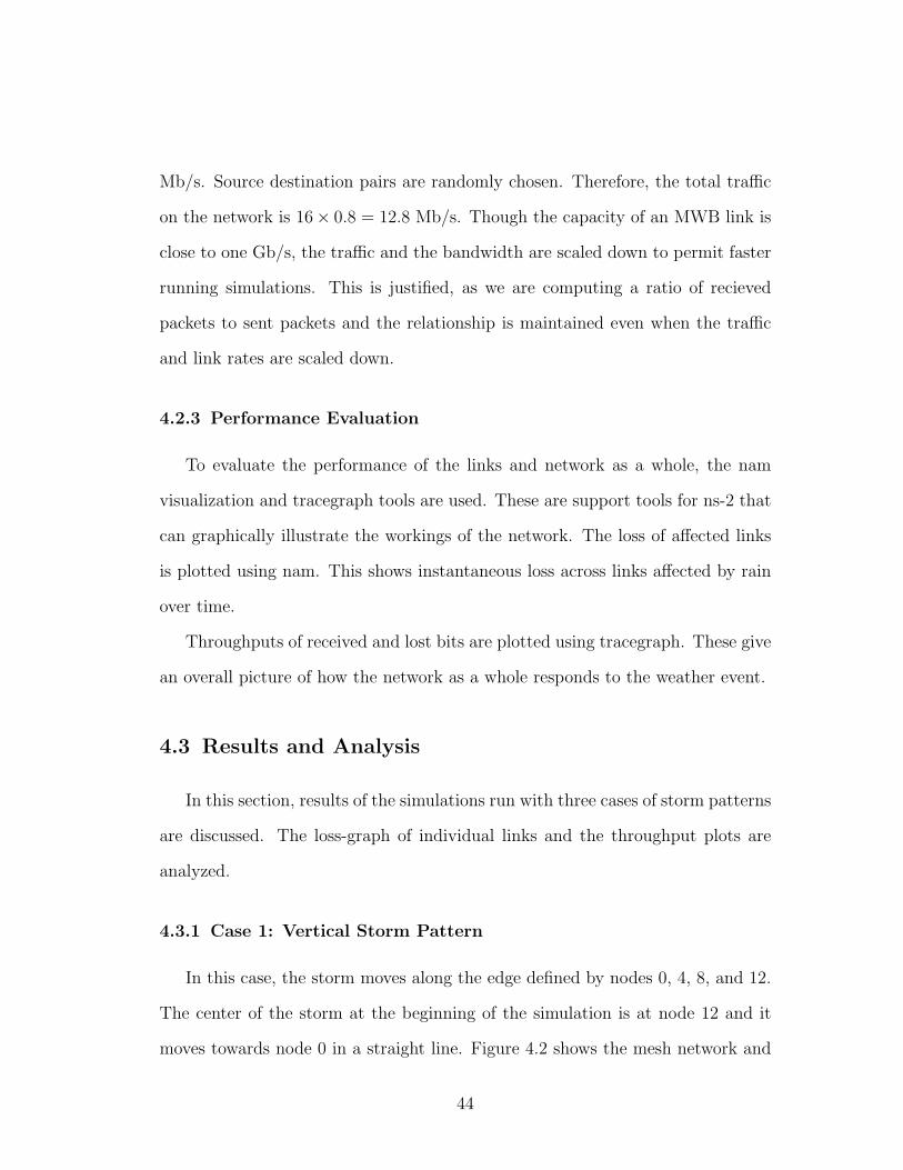
4.2.3 Performance Evaluation

To evaluate the performance of the links and network as a whole, the nam

visualization and tracegraph tools are used. These are support tools for ns-2 that

can graphically illustrate the workings of the network. The loss of affected links

is plotted using nam. This shows instantaneous loss across links affected by rain

over time.

Throughputs of received and lost bits are plotted using tracegraph. These give

an overall picture of how the network as a whole responds to the weather event.

4.3 Results and Analysis

In this section, results of the simulations run with three cases of storm patterns

are discussed. The loss-graph of individual links and the throughput plots are

analyzed.

4.3.1 Case 1: Vertical Storm Pattern

In this case, the storm moves along the edge defined by nodes 0, 4, 8, and 12.

The center of the storm at the beginning of the simulation is at node 12 and it

moves towards node 0 in a straight line. Figure 4.2 shows the mesh network and

44

the structure and trajectory of the storm for Case 1. Each position of the storm is

one second apart and the duration of the simulation is approximately 60 seconds.

Figure 4.2. Case 1: Storm moves along the edge of a network

Figure 4.3 shows the loss on the affected links, in particular between nodes 12

and 13, 8 and 12, 9 and 8, 8 and 4, 4 and 5, 0 and 4, and 0 and 1.

45

Figure 4.3. Case 1: Packets lost across affected links

The storm enters at node 12 and gradually moves to node 0. The orientation

of the inner ellipse is such that it cuts the horizontal links at regular intervals.

The vertical edge-links are not affected by the inner ellipses and therefore are

under the influence of only the bigger ellipse. As the storm moves in a straight

line perpendicular to the x-axis, there is a pattern of losses across links which is

clearly seen in Figure 4.3. The link composed of node pair (12,13) gets affected at

the beginning of the simulation as the inner ellipse is centered in the middle of the

link. The loss on it gradually decreases and finally becomes zero when the storm

system has completely passed. The horizontal links (12,13), (8,9), (4,5), and (0,1)

show an identical pattern while the vertical links (12,8) (8,4) (12,8) show another

pattern albeit identical.

As the storm pattern is regular and most parts of the network are not affected

by the storm, the degradation in throughput is of the order of five per cent. From

the tracegraph utility, we obtain the number of packets sent (Ns) and the number

of packets dropped (Nd). Using this, the carried load of the network (η) can be

calculated as:

η =Ns −Nd

Nd

× 100% (4.1)

46

For this case, Ns = 171,288 and Nd = 7,728 resulting in a carried load value

of η = 95.488%. The average throughput is 11.8 Mb/s compared to 12.8 Mb/s

for the ideal case.

Table 4.1. Case 1: Simulation information

Simulation length in seconds: 55.19715

Number of nodes: 16

Number of sending nodes: 16

Number of receiving nodes: 16

Number of generated packets: 176640

Number of sent packets: 171288

Number of forwarded packets: 301392

Number of dropped packets: 7728

Number of lost packets: 2376

Minimal packet size: 500

Maximal packet size: 500

Average packet size: 500

Number of sent bytes: 85644000

Number of forwarded bytes: 150696000

Number of dropped bytes: 3864000

Packets dropping nodes: 0 4 6 12

Table 4.1 shows the details of the simulation for Case 1. Figure 4.4 shows the

throughput of all the bits received by all the nodes in the network. It is seen that

there is a pattern in the total traffic through the network. Figure 4.5 shows the

throughput of all the dropped bits in the network.

47

Figure 4.4. Case 1: Throughput of all received bits

Figure 4.5. Case 1: Throughput of all dropped bits

4.3.2 Case 2: Diagonal Storm Pattern

In this case, the storm starts at node 12 and moves along the principal diagonal

to reach node 3 at the end of the simulation. The orientation of the storm cells is48

45◦ with respect to the positive x-axis.

Figure 4.6. Case 2: Storm moves diagonally across the network

Table 4.2 shows the simulation information for Case 2. In this case, Ns =

145,413 and Nd = 15,946, resulting in a carried load value of η = 89.903% which is

worse than the first case. This is intuitive because the second storm simultaneously

affects more links than the first storm. The average throughput is 10.97 Mbps

compared to 12.8 Mbps for the ideal network.

Figure 4.7 shows the throughput of all the received bits and Figure 4.8 shows

49



Number of nodes: 16














Packets dropping nodes: 2 5 6 8 9 10 12 13

all the dropped bits. These plots are not as intuitive as the ones for the first case

because the storm is moving diagonally and the individual cells are aligned at 45◦

from the positive x-axis.

4.3.3 Case 3: Diagonal Pattern with Larger Storm

In this case, the second storm pattern is used in which the storm starts centered

at node 12 and moves along the principal diagonal to reach node 0, but the ellipse

parameters are changed. The bigger ellipse has a larger major-axis diameter of

30 km and minor axis diameter of 20 km. The inner ellipses each have major-axis

50



diameters of nine km and minor axis diameters of five km. Figure 4.9 shows the

movement of this storm across the 4× 4 mesh. As the storm covers more links at

51

0 1 2 3

4 5 6 7

8 9 10 11

12 13 14 15

61

0 1 2 3

4 5 6 7

8 9 10 11

12 13 14 15

0 1 2 3

4 5 6 7

8 9 10 11

12 13 14 15

0 1 2 3

4 5 6 7

8 9 10 11

12 13 14 15

0 1 2 3

4 5 6 7

8 9 10 11

12 13 14 15

0 1 2 3

4 5 6 7

8 9 10 11

12 13 14 15

0 1 2 3

4 5 6 7

8 9 10 11

12 13 14 15

0 1 2 3

4 5 6 7

8 9 10 11

12 13 14 15

0 1 2 3

4 5 6 7

8 9 10 11

12 13 14 15

0 1 2 3

4 5 6 7

8 9 10 11

12 13 14 15

0 1 2 3

4 5 6 7

8 9 10 11

12 13 14 15

0 1 2 3

4 5 6 7

8 9 10 11

12 13 14 15

0 1 2 3

4 5 6 7

8 9 10 11

12 13 14 15

0 1 2 3

4 5 6 7

8 9 10 11

12 13 14 15

0 1 2 3

4 5 6 7

8 9 10 11

12 13 14 15

0 1 2 3

4 5 6 7

8 9 10 11

12 13 14 15

0 1 2 3

4 5 6 7

8 9 10 11

12 13 14 15

0 1 2 3

4 5 6 7

8 9 10 11

12 13 14 15

0 1 2 3

4 5 6 7

8 9 10 11

12 13 14 15

0 1 2 3

4 5 6 7

8 9 10 11

12 13 14 15

0 1 2 3

4 5 6 7

8 9 10 11

12 13 14 15

0 1 2 3

4 5 6 7

8 9 10 11

12 13 14 15

0 1 2 3

4 5 6 7

8 9 10 11

12 13 14 15

0 1 2 3

4 5 6 7

8 9 10 11

12 13 14 15

0 1 2 3

4 5 6 7

8 9 10 11

12 13 14 15

0 1 2 3

4 5 6 7

8 9 10 11

12 13 14 15

0 1 2 3

4 5 6 7

8 9 10 11

12 13 14 15

0 1 2 3

4 5 6 7

8 9 10 11

12 13 14 15

0 1 2 3

4 5 6 7

8 9 10 11

12 13 14 15

0 1 2 3

4 5 6 7

8 9 10 11

12 13 14 15

0 1 2 3

4 5 6 7

8 9 10 11

12 13 14 15

0 1 2 3

4 5 6 7

8 9 10 11

12 13 14 15

0 1 2 3

4 5 6 7

8 9 10 11

12 13 14 15

0 1 2 3

4 5 6 7

8 9 10 11

12 13 14 15

0 1 2 3

4 5 6 7

8 9 10 11

12 13 14 15

0 1 2 3

4 5 6 7

8 9 10 11

12 13 14 15

0 1 2 3

4 5 6 7

8 9 10 11

12 13 14 15

0 1 2 3

4 5 6 7

8 9 10 11

12 13 14 15

0 1 2 3

4 5 6 7

8 9 10 11

12 13 14 15

0 1 2 3

4 5 6 7

8 9 10 11

12 13 14 15

0 1 2 3

4 5 6 7

8 9 10 11

12 13 14 15

0 1 2 3

4 5 6 7

8 9 10 11

12 13 14 15

0 1 2 3

4 5 6 7

8 9 10 11

12 13 14 15

0 1 2 3

4 5 6 7

8 9 10 11

12 13 14 15

0 1 2 3

4 5 6 7

8 9 10 11

12 13 14 15

0 1 2 3

4 5 6 7

8 9 10 11

12 13 14 15

0 1 2 3

4 5 6 7

8 9 10 11

12 13 14 15

0 1 2 3

4 5 6 7

8 9 10 11

12 13 14 15

0 1 2 3

4 5 6 7

8 9 10 11

12 13 14 15

0 1 2 3

4 5 6 7

8 9 10 11

12 13 14 15

0 1 2 3

4 5 6 7

8 9 10 11

12 13 14 15

0 1 2 3

4 5 6 7

8 9 10 11

12 13 14 15

0 1 2 3

4 5 6 7

8 9 10 11

12 13 14 15

0 1 2 3

4 5 6 7

8 9 10 11

12 13 14 15

0 1 2 3

4 5 6 7

8 9 10 11

12 13 14 15

0 1 2 3

4 5 6 7

8 9 10 11

12 13 14 15

0 1 2 3

4 5 6 7

8 9 10 11

12 13 14 15

0 1 2 3

4 5 6 7

8 9 10 11

12 13 14 15

0 1 2 3

4 5 6 7

8 9 10 11

12 13 14 15

0 1 2 3

4 5 6 7

8 9 10 11

12 13 14 15

0 1 2 3

4 5 6 7

8 9 10 11

12 13 14 15

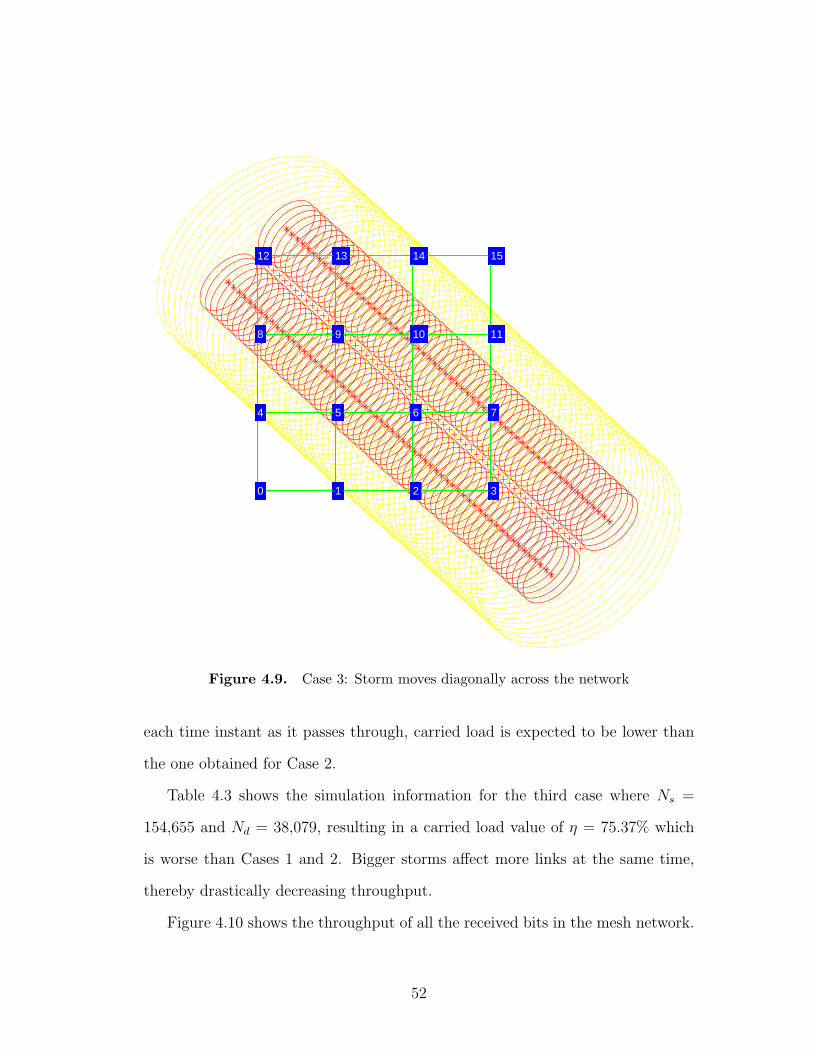
Figure 4.9. Case 3: Storm moves diagonally across the network

each time instant as it passes through, carried load is expected to be lower than

the one obtained for Case 2.

Table 4.3 shows the simulation information for the third case where Ns =

154,655 and Nd = 38,079, resulting in a carried load value of η = 75.37% which

is worse than Cases 1 and 2. Bigger storms affect more links at the same time,

thereby drastically decreasing throughput.

Figure 4.10 shows the throughput of all the received bits in the mesh network.

52



Number of nodes: 16














Packets dropping nodes: 1 2 4 5 6 8 9 10 12 13

The average throughput is 8.76 Mbps compared to the ideal case of 12.8 Mbps.

Figure 4.11 shows the throughput of all the dropped bits for Case 3.

It is seen that even mild rain rates of two mm/h and heavier rain rates of

10 mm/h cause a 10% drop in throughput. Bigger and more intense storms can

deteriorate links to the extent of causing complete link outage.

53



54

Chapter 5

Link Modeling

Long-term statistics of rain attenuation are useful for planning link budgets

and determining the automatic gain control (AGC) in MWB transceivers [35,36].

Links are often designed with a knowledge of rain-rate statistics by performing

a rain-rate time-series to attenuation time-series conversion [28]. But, when a

test link is available, the approximation from rain rate to attenuation becomes

needless. A model can be constructed with attenuation measurements obtained

directly from the transceivers on the link. In this thesis, one such model is pre-

sented.

We propose a three-state Markov model of a link based on FER measurements.

The three states, strong, weak and disconnected, each represent a particular range

of values of FER. Measured values of FER are categorized into strongly connected,

weakly connected or disconnected, based on the thresholds set for each state. A

Markov model is then formulated, either for a specific time period such as a stormy

day, or for the lifetime of the link. This is discussed in detail in Section 5.3.

This chapter is organized as follows: Markov processes are explained in Sec-

tion 5.1, the measurement setup is explained in Section 5.2, and the three-state

55

model is presented in Section 5.3.

5.1 Markov Process

A Markov process is a particular type of stochastic process in which knowledge

of the present state is necessary and sufficient to describe the future state. In other

words, the future states are independent of the past states and are dependent only

on the present state, referred to as memoryless.

Each state represents a random variable Xi = {X1,X2,X3. . .Xn} where n

denotes the number of states and Xi. . .Xn are random variables with the following

property:

P{Xi = x/Xi−1. . .X1} = P{Xi = x/Xi−1} 1 ≤ i ≤ n (5.1)

The probability of the system to be in a particular state is the state probability,

and the probability of the system to go from one state to another is the state-

transition probability. Markov processes are widely used in a variety of applications

including building models for weather prediction. In this case, a simple two-state

link is considered where the states are strong and disconnected. The transition

probability matrix (TPM) for the two-state link is:

P =

p11 p12

p21 p22

=

0.7 0.3

0.6 0.4

(5.2)

where, p11 is the probability that the current state of the link is strong given it

was strong in the previous time instant, p12 is the probability that the current

state of the link is weak given it was strong in the previous time instant, p21 is

56

the probability that the current state of the link is strong given it was weak in the

previous time instant, and p22 is the probability that the current state of the link

is weak given it was weak in the previous time instant. The following is a very

important property of the TPM:

n∑j=1

pij = 1 ∀ i ∈ {1....n} (5.3)

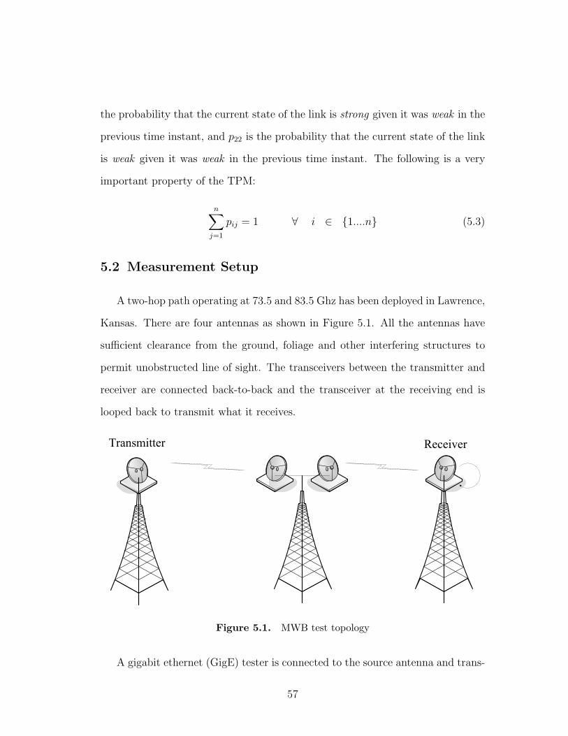
5.2 Measurement Setup

A two-hop path operating at 73.5 and 83.5 Ghz has been deployed in Lawrence,

Kansas. There are four antennas as shown in Figure 5.1. All the antennas have

sufficient clearance from the ground, foliage and other interfering structures to

permit unobstructed line of sight. The transceivers between the transmitter and

receiver are connected back-to-back and the transceiver at the receiving end is

looped back to transmit what it receives.

Figure 5.1. MWB test topology

A gigabit ethernet (GigE) tester is connected to the source antenna and trans-

57

mits 512-byte packets in 30-second intervals at roughly one Gb/s. The GigE tester

records parameters such as number of transmitted packets, number of dropped

packets, latency, and standard deviation of the latency. FER (frame error ratio)

is calculated from the knowledge of transmitted and dropped packets and the link

is categorized into the strong/weak/disconnected states based on certain threshold

values for every time interval. If Ns is the number of packets sent and Nd is the

number of packets dropped, then FER is given by:

FER =

(Nd

Ns

)(5.4)

and the thresholds are defined as follows:

• strongly connected if FER < Ts

• weakly connected if Ts ≤ FER ≤ Td

• disconnected if FER > Td

where Ts is the threshold for strongly connected and Td is the threshold for dis-

connected.

From this, a Markov model is constructed and state and state-transition prob-

abilities are calculated. These numbers can be calculated on any time frame of

choice. The most useful ones include monthly figures for analyzing worst-month

statistics and days that had significant rainfall, both of which help in planning

link budgets for a particular geographical area, as weather phenomena are local

in nature.

58

p21

p12 p31

p33 p22

p11

p13

p23

p32

1

2 3

1 - Strongly Connected2 - Weakly Connected3 - Disconnected

SC

WC DC

Figure 5.2. Three-state Markov model of link states

5.3 Three-State Markov Model

If we quantize the performance of the link to three states: strong, weak, and

disconnected, then the Markov model in Figure 5.2 represents the system. States

one, two, and three correspond to the states strong, weak, and disconnected re-

spectively and pij represents the transition probability from state i to state j and

is defined as:

pij = P{Xt+1 = j/Xt = i} (5.5)

59

0 200 400 600 800 1000 1200 1400 1600 1800 200010

−7

10−6

10−5

10−4

10−3

10−2

10−1

100

Sample number (taken approximately every 30 seconds)

Fram

e er

ror

ratio

Strong

Weak

Disconnected

Figure 5.3. Quantization of link performance to three levels

where X is the random variable used to represent the state of the link and

i, j ∈ {1, 2, 3}. For example, for the case shown in Figure 5.3, the thresholds set

are:

• strongly connected if FER < 10−6

• weakly connected if 10−6 ≤ FER ≤ 10−2

• disconnected if FER > 10−2

Table 5.1 shows the state probabilities for the strong, weak, and disconnected

states and Table 5.2 shows the transition probabilities between the three states

for FER measured over a rainy 24-hour period in June 2007. The thresholds

used to calculate the probability values are specified. It is seen that changing the

thresholds changes the transition probability values. If the availability required is

60

Table 5.1. 24-hour state probabilities without FEC (Jun. 2007)

State Probability

Strong 0.2159

Weak 0.7614

Disconnected 0.0225

Table 5.2. 24-hour TPM without FEC (Jun. 2007)

State Strong Weak Disconnected

Strong 0.9846 0.0127 0.0025

Weak 0.0036 0.9905 0.0057

Disconnected 0.0487 0.1707 0.7804

high, stricter bounds for strong, weak, and disconnected states can be established.

These probability values will then show how long the link stays in a particular

state and how often it transitions into other states. In the past, monthly and

yearly statistics were typically used in formulating link budgets. But from the

measurement results, it is seen that the availability requirements are not met (For

carrier grade, it is usually 99.9% to 99.999% or higher.). In this case, the statistics

of a rainy day may be very important to meet availability requirements.

Table 5.3. State probabilities with FEC (Jul. 2007–Feb. 2008)

State Probability

Strong 0.9469

Weak 0.0255

Disconnected 0.0275

61

Table 5.4. TPM with FEC (Jul. 2007–Feb. 2008)


Strong 0.9869 0.0124 0.0005

Weak 0.4666 0.4965 0.0368

Disconnected 0.0162 0.0383 0.9454

Table 5.3 and Table 5.4 show the state probabilities and state-transition prob-

abilities for FER measurements made on a set of transceivers with forward error

correction (FEC) between July 2007 and February 2008. Table 5.5 and Table 5.6

show the state and state-transition probabilities for FER measured on transceivers

without FEC over the same time period. It is seen that the strong state proba-

bility is much higher with FEC. The transceivers with FEC use a Reed Solomon

204/188 FEC. In both cases, the links do not perform ARQ (automatic repeat

request); this is the current practice in commercial MWB equipment.

Table 5.5. State probabilities without FEC (Jul. 2007–Feb. 2008)

State Probability

Strong 0.3864

Weak 0.5303

Disconnected 0.0833

Table 5.6. TPM without FEC (Jul. 2007 – Feb. 2008)


Strong 0.9364 0.0633 0.0003

Weak 0.0461 0.9490 0.0049

Disconnected 0.0015 0.0310 0.9675

62

Steady state values of models like the one described here can be used to gen-

erate rain-attenuation time-series [28, 37, 38]. Simulation of rain-rate time-series

from the state and state-transition probabilities depends on the duration of atten-

uation measurement. To simulate isolated rain events or stormy days, the values in

Tables 5.1 and 5.2 can be used. In the past, if statistics were required for planning

link budgets, worst-month statistics or measurements taken over a longer dura-

tion were used. In this case, data is available over eight months, which is used

to reasonably predict the availability of the link. These models can be trained by

including more data in the calculations. In general, the availability of a link is

better when the entire year is taken into account compared to rainy months, but

that is not useful in designing links that meet availability requirements. Designing

a link with the availability numbers obtained from yearly statistics might cause

complete outage of the link during the rainy months. Therefore, the month in

which availability is the worst is chosen and the links and network are planned

accordingly. Using maximum transmit power, gain of the antennas, and narrow

band signals does not help because the network is made of multiple links and all

these will lead to interference. The transmission parameters of the transceivers

are changed in some cases and in others, multi-hop paths are used instead of one

long link. Multi-hop paths may not be an efficient solution always because of cost

factors.

The weak and disconnected state probabilities can help adjust design param-

eters to increase the availability of the link and the network. If a link is in the

weak state for a significant portion of the time (50% in the transceivers without

FEC), changing design parameters might result in better availability results. It

should be noted that all design decisions must comply with the criteria specified

63

by the FCC presented in Section 2.1.1.

The availability of the transceivers with FEC is ∼94% whereas that of the

transceivers without FEC is ∼38%. Though their specifications are different (The

transceivers without FEC use two-foot diameter antennas and the ones with FEC

use one-foot diameter antennas and they operate at frequencies one GHz apart.),

the comparison is not unfair because they are commercial equipment with similar

availability specifications. The availability calculated from FER measurements is

significantly different. One of the major causes of this, apart from rain, might

be the fact that the transceiver without FEC has a two-foot diameter antenna

and a beamwidth of 0.6◦ and therefore will be affected more by error-angle fading

and signal loss due to tower sway. Adding Reed-Solomon 204/188 FEC on this

transceiver might make the comparison fairer.

64

Chapter 6

Conclusions and Future Work

Attenuation due to rain is a serious issue in MWB links. If a metropolitan mesh

network or a backhaul network is built using MWB links, weather effects have to be

considered while planning the link budget as they significantly impact availability

figures. Long-term statistics help plan link budgets, but are hardly useful on an

event-by-event basis. In the event of rain, network throughput and carried load

can be severely affected as shown in Chapter 4. Knowledge of the spatio-temporal

effects of rain on the links in a mesh network is required to calculate throughput

and efficiency reduction or to implement intelligent routing schemes. This thesis

work has presented a method to model the spatio-temporal effects of rain on a

mesh network and evaluate network performance in the event of rain and other

atmospheric impairments.

To reiterate, the contributions of this research work are:

• Developed a synthetic storm model with structure and trajectory, which

represents the characteristics of a real-world storm, and modeled the effects

of the storm on an MWB mesh network.

65

• Simulated the effects of rain attenuation on network performance using ns-2.

• Formulated long-term statistics of rain attenuation using a three-state Markov

model. The model is built from actual measurements of frame error rates

on a physical link.

In this chapter, conclusions inferred from this work and future enhancements that

will improve this work are presented.

6.1 Conclusions

The mass deployment of MWB links depends a lot on our understanding of the

effects of atmospheric impairments such as rain on MWB transmissions. Though

empirical models prove satisfactory for initial assesment, they are not sufficient

for network planning and link budgeting.

This work provides a means of incorporating spatio-temporal effects of rain in a

MWB mesh network and a mathematical model derived from actual measurements

that provides long-term statistics of the MWB link.

It is seen that approximating the structure of storm cells to ellipses and asso-

ciating a rain rate to each ellipse according to the intensity of the cell, provides a

reasonable method of calculating attenuation across multiple links in a mesh net-

work during a rain event. The movement of the rain cells is also captured, which

ensures that each link captures different rain rates at different times, similar to a

real life scenario.

The ns-2 simulations prove that a rain event with typical intensity can lead to

link outage, therefore, static routing is not sufficient to meet the required avail-

ability and reliability standards. Dynamic routing or predictive routing schemes

66

must be employed if availability in excess of 99% is desired.

The state probability matrices obtained from measurements show that the link

is weak for a significant fraction of time. It is possible to move the link to the

strong state by modifying parameters such as bandwidth of the link, transmit

power, gain of the transmitting and receiving antennas, and modulation schemes.

From the state-transition probability matrices, it is seen that it is not unlikely for

the link to transition between extreme states.

6.2 Future Work

The basic premise of this research work is that storm cells are elliptical in

nature with the smaller ellipses non overlapping and completely contained within

the bigger ellipse.

The trajectory of the storm is the locus of the center of the system. The cells

move relative to the center of the system and do not have trajectories of their

own. This is not the case in real life as the cells and their front typically have

different trajectories.

The storm is modeled as one big ellipse with several smaller ellipses contained

within it. It is possible to have storm systems with more than one big ellipse.

The ITU model relating attenuation and rain rate is used in this work. Instead,

a relationship curve can be plotted with the results of measurements of rain and

FER on the physical link setup. From the curve, a table lookup can be done to give

a particular value of attenution/FER for a given value of rain rate that is readily

available from radar data and rain gauges. This would be more accurate than the

ITU model for the region in which the measurements are made. But measurements

over a long period of time and a wide range of rain-rate values would be required

67

to do this. Figure 6.1 shows a preliminary plot of FER measured and derived

from the ITU-R P.838-3 recommendation.

Figure 6.1. Measured FER vs. FER derived from ITU-R P. 838-3

All nodes in the network are set to transmit and receive at the same frequency.

Though this assumption is reasonable considering the properties of MWB trans-

missions in the real world, transceivers will operate at different bands within the

MWB. For more accurate results, this must be considered.

In a mesh network operating at MWB, intelligent routing schemes could be

devised to circumvent the problems caused by rain attenuation and make efficient

use of the links in the network. Exploring different routing schemes to find optimal

68

solutions is an excellent problem that needs to be addressed.

The Markov model built to measure long-term probabilities of attenuation uses

3 states: strong, weak, and disconnected. The number of states can be increased

and the thresholds can be modified to obtain better resolution if needed.

69

Appendix A

ITU-R P.838-3 Coefficients

Table A.1. Coefficients for kH

j aj bj cj mk ck

1 -5.33980 -0.10008 1.13098

-0.18961 0.711472 -0.35351 1.26970 0.45400

3 -0.23789 0.86036 0.15354

4 -0.94158 0.64552 0.16817

Table A.2. Coefficients for kV

j aj bj cj mk ck

1 -3.80595 0.56934 0.81061

-0.16398 0.632972 3.44965 -0.22911 0.51059

3 -0.39902 0.73042 0.11899

4 0.50167 1.07319 0.27195

70

Table A.3. Coefficients for αH

j aj bj cj mα cα

1 -0.14318 1.82442 -0.55187

0.67849 -1.95537

2 0.29591 0.77564 0.19822

3 0.32177 0.63773 0.13164

4 -5.37610 -0.96230 1.47828

5 16.1721 -3.29980 3.43990

Table A.4. Coefficients for αV

j aj bj cj mα cα

1 -0.07771 2.33840 -0.76284

-0.053739 0.83433

2 0.56727 0.95545 0.54039

3 -0.20238 1.14520 0.26809

4 -48.2991 0.791669 0.116226

5 48.5833 0.791459 0.116479

71

References

[1] GigaBeam Corporation. New Spectrum Bands Enable GigaBeam’s WiFiber

Revolution. [Online]. Available: http://www.gigabeam.com/technology.cfm

[2] FCC, “Millimeter Wave Propagation: Spectrum Management Implications,”

Bulletin Number 70, 1997.

[3] Mike Willis. Absorption by Atmospheric Gases. [Online]. Available:

{http://www.mike-willis.com/Tutorial/gases.htm}

[4] W. Myers, “Comparison of Propagation Models,” IEEE P802.16 Broadband

Wireless Access Working Group, 1999. [Online]. Available: {http:

//www.ieee802.org/16/tg2\ orig/contrib/80216cc-99\ 13.pdf}

[5] Cisco Systems Inc. (May 16,2003) 02-146 ExParte FCC WTB. [Online].

Available: {http://www.gigabeam.com/FCC\ Information/Cisco\ FCC\

ExParte\ Filing\ May\ 16\ 2003.pdf}

[6] D. Lockie, “Upper Millimeter-wave History, Technology and Applications

for Gigabit Class Communications Service,” IEEE 802 LMSC Plenary

Session, 2002. [Online]. Available: {http://www.ieee802.org/802\ tutorials/

march02/T80216-02\ 02b.pdf}

72

[7] Information Sciences Institute, “NS-2 Network Simulator,” Software

Package, 2003. [Online]. Available: {http://www.isi.edu/nsnam/ns/}

[8] “Allocations and Service Rules for the 71-76 GHz, 81-86 GHz and 92-95 GHz

Bands,” Memorandum and Opinion Order (FCC 03–248), 2003.

[9] “Allocations and Service Rules for the 71-76 GHz, 81-86 GHz and 92-95 GHz

Bands,” Memorandum and Opinion Order (FCC 05–45), 2005.

[10] R. A. Nelson. Antennas. [Online]. Available: {http://www.aticourses.com/

antennas\ tutorial.htm}

[11] T. S. Rappaport, Wireless Communications: Principles and Practice. Pear-

son Education Inc., 2004, pp. 126–128.

[12] Comite Consultatif International pour la Radio, “Propagation in Non-ionized

Media,” in Recommendations and Reports of the CCIR,Vol. V, 1990.

[13] G. Brussard and P. Watson, Atmospheric Modelling and Millimeter Wave

Propagation. Chapman and Hall, London, 1995.

[14] Y.Yan, “Microwave Propagation in Saline Dust Storms,” International Jour-

nal of Infrared and Millimeter Waves, vol. 25 No. 8, pp. 1337–1243, 2004.

[15] T. Garlington, “Millimeter E-Band Radio,” US Army Information Systems

Engineering Command, 2006. [Online]. Available: {http://www.hqisec.army.

mil/isec/publications/Millimeter\ Wave\ E-Band\ Radio\ May06.pdf}

[16] “Effects of Tropospheric Refraction on Radiowave Propagation,” in CCIR

Report 718-2, vol. 5, 1986.

73

[17] G. S. Feldhake and L. Ailes-Sengers, “Comparison of Multiple Rain Attenu-

ation Models with Three Years of Ka Band Propagation Data Concurrently

Taken at Eight Different Locations,” Online Journal of Space Communica-

tion, vol. 2, 2002.

[18] C. E. Mayer and B. E. Jaeger, “Rain Attenuation Model Comparison and

Validation,” Online Journal of Space Communication, vol. 2, 2002.

[19] R. K.Crane, Electromagnetic Wave Popagation Through Rain. John Wiley

& Sons Inc., 1996, pp. 139–184.

[20] R. K. Crane, “Prediction of Attenuation by Rain,” IEEE Transactions on

Communications, vol. 28, pp. 1717–1733, 1980.

[21] “Specific Attenuation Model for Rain for use in Prediction Methods,” Rec-

ommendation ITU-R P.838-3, 1992–1999–2003–2005.

[22] Bridgewave Communications. Extended-Range Wireless Gigabit Ethernet

Link Model GE60X. [Online]. Available: {http://www.commconnect.com/

documents/GE60X\ Datasheet.pdf}

[23] G. Hendrantoro, Indrabayu, T. Suryani, and A. Mauludiyanto, “A Multi-

variate Autoregressive Model of Rain Attenuation on Multiple Short Radio

Links,” IEEE Antennas and Wireless Propagation Letters, vol. 5, pp. 54–57,

2006.

[24] A. Dissanayake, J. Allnutt, and F. Haidara, “A Prediction Model that Com-

bines Rain Attenuation and Other Propagation Impairments along Earth-

Satellite Paths,” Online Journal of Space Communication, 2002.

74

[25] T. Utsunomiya and M. Sekine, “Rain Attenuation at Millimeter and Sub-

millimeter Wavelengths,” International Journal of Infrared and Millimeter

Waves, vol. 26, no. 6, pp. 905–920, 2005.

[26] C. Alasseur, A. Nunez, F. Fontan, L. Husson, U.-C. Fiebig, and P. Marino,

“Two approaches for effective modelling of rain-rate time-series for radiocom-

munication system simulations,” Space Communications, vol. 20, no. 1–2, pp.

69–83, 2005.

[27] M. Montopoli, F. S. Marzano, G. Vulpiani1, A. Fornasiero, P. P. Alberoni,

L. Ferraris, and N. Rebora, “Spatial Characterization of Raincell Horizontal

Profiles from C-band Radar Measurements at Mid-latitude,” Advances in

GeoSciences, vol. 7, pp. 285–292, 2006.

[28] F. Fontan, A.Nunez, A. Valcarce, and U.C.Fiebig, “Converting Simulated

Rain-rate Series into Attenuation Series Using the Synthetic Storm Tech-

nique,” in 3rd International Workshop on Propagation Impairment Mitiga-

tion for Millimeter Wave Radio Systems, 2005.

[29] A.Daru, Z. Kormanyos, and J.Bito, “Space and Time Correlation of Rain

Attenuation in Millimeter Wave Feeder Network,” in COST Action 280 1st

International Workshop, July 2002.

[30] C. Riva, “Spatial Characteristics of Propagation Parameters: A Review,” in

COST Action 280 1st International Workshop, July 2002.

[31] G. C. Pomraning, “Transport Theory in Discrete Stochastic Mixtures,” in

Advances in Nuclear Science and Technology, vol. 24. Springer US, 1996,

pp. 47–93.

75

[32] B. Su and G. C. Pomraning, “A Stochastic Description of a Broken Cloud

Field,” Journal of Atmospheric Sciences, vol. 51, pp. 1969–1977, 1993.

[33] A. Kassler, M. Castro, and P. Dely, “VoIP Packet Aggregation based on

Link Quality Metric for Multihop Wireless Mesh Networks,” in Cost 290 6th

MCM, 2007.

[34] J. Postel, “User Datagram Protocol,” in RFC 768, 1980.

[35] M. R. Islam, “Frequency Scaling Technique for Rain Attenuation Prediction

on Terrestrial Microwave Links in Tropical Climate,” in ICECE 2002, De-

cember,2002, pp. 372–375.

[36] K. S. Paulson and J. W. F. Goddard, “Report on Link Reliability

Project: Winchester and Thorne Hill,” Project Report D36-5, July,2002.

[Online]. Available: http://www.ofcom.org.uk/static/archive/ra/topics/

research/rcru/project36/WinchThornD36-5.pdf

[37] M. van de Kamp, “Rain Attenuation as a Markov Process: The Meaning of

Two Samples,” in COST Action 280 1st International Workshop, July 2002.

[38] P. Hou, J. Zhuang, and G. Zhang, “A Rain Fading Simulation Model for

Broadband Wireless Access Channels in Millimeter Wavebands,” 51st Vehic-

ular Technology Conference, pp. 2559–2563, 2000.

76

Documents

Synthetic Storm Modeling for Millimeter Wave Band Mesh Networks