57Synchrophasors: Definition, Measurement, and Application

1. Abstract

The concept of using phasors to describe power system operating quantities dates back to 1893 and Charles Proteus Steinmetz’s paper on mathematical techniques for analyzing AC networks1. More recently, Steinmetz’s technique of phasor calculation has evolved into the calculation of real-time phasor measurements synchronized to an absolute time reference.

Although phasors have been clearly understood for over 100 years, the detailed definition of a time-synchronized phasor has only recently been codified in the IEEE 1344 and the soon-to-be voted IEEE C37.118 Synchrophasor for Power Systems standards. This paper will review the concept of a phasor and examine the proposed IEEE standard as to “how” a synchronized phasor is to be defined, time stamped, and communicated.

The paper will then examine the issues of implementing such measurements in the face of off-nominal frequency components, timing errors, sensor errors, and system harmonics. Simulations of various system transients and their phasor responses will be presented. Finally, this paper will review the application of synchrophasors to observe power system dynamic phenomena and how they will be used in the real-time control of the power system. Examples of system disturbances will also be presented.

2. Introduction

As the electric power grid continues to expand and as transmission lines are pushed to their operating limits, the dynamic operation of the power system has become more of a concern and has become more difficult to accurately model. In addition, the ability to effect real-time system control is developing into the need to prevent wide scale cascading outages.

For decades, control centers have estimated the “state” of the power system (the positive sequence voltage and angle at each network node) from measurements of the power flows through the power grid. It is very desirable to be able to “measure” the system state directly and/or augment existing estimators with additional information.

Alternating Current (AC) quantities have been analyzed for over 100 years using a construct developed by Charles Proteus Steinmetz in 1893, known as a “phasor.” On the power system, phasors were used for analyzing AC quantities assuming a constant frequency. A relatively new variant of this technique

that synchronizes the calculation of a phasor to absolute time has been developed2, known as “synchronized phasor measurement” or “synchrophasors.” In order to uniformly create and disseminate these synchronized measurements, several aspects of phasor creation had to be codified3. The following spells out the definitions and requirements that have been established for the creation of synchronized phasor measurements.

3. Synchrophasor Definition

An AC waveform can be mathematically represented by the equation:

Note that the synchrophasor is referenced to the cosine function. In a phasor notation, this waveform is typically represented as:

Since in the synchrophasor definition, correlation with the equivalent RMS quantity is desired, a scale factor of 1/ 2 must be applied to the magnitude which results in the phasor representation as:

Adding in the absolute time mark, a synchrophasor is defined as the magnitude and angle of a cosine signal as referenced to an absolute point in time as shown in Figure 1.

In Figure 1, time strobes are shown as UTC Time Reference 1 and UTC Time Reference 2. At the instant that UTC Time Reference 1 occurs, there is an angle shown as “+q” and, assuming a steady-state sinusoid (i.e. – constant frequency), there is a magnitude of the waveform of X1. Similarly, at UTC Time Reference 2, an angle, with respect to the cosine wave, of “-q” is measured along with a magnitude or X2. The measured angle is required to be reported in the range of ± p. It should be emphasized that the

Synchrophasors:Definition, Measurement, and Application

Mark AdamiakGE Multilin

King of Prussia, PA

William PremerlaniGE Global Research

Niskayuna, NY

Dr. Bogdan KasztennyGE Multilin

Markham, Ontario

58 Synchrophasors: Definition, Measurement, and Application

synchrophasor standard focuses on steady-state signals, that is, signals wherein the frequency of the waveform is constant over the period of measurement.

In the real world, the power system seldom operates at exactly the nominal frequency. As such, the calculation of the phase angle, q, needs to take into account the actual frequency of the system at the time of measurement. For example, if the nominal frequency is 59.5Hz on a 60Hz system, the period of the waveform is 16.694ms instead of 16.666ms – a difference of 0.167%.

The captured phasors are to be time-tagged based on the time of the UTC Time Reference. The Time Stamp is an 8-byte message consisting a 4 byte “Second Of Century – SOC”, a 3-byte Fraction of Second and a 1-byte Time Quality indicator. The SOC time-tag counts the number of seconds that have occurred since January 1, 1970 as an unsigned 32-bit Integer. With 32 bits, the SOC counter is good for 136 years or until the year 2106.

With 3-bytes for the Fraction Of Second, one second can be broken down into 16,777,216 counts or about 59.6 nsec/count. If such resolution is not desired, the proposed standard (C37.118) allows for a user-definable base over which the count will wrap (e.g. – a base of 1,000,000 would tag a phasor to the nearest microsecond).

Finally, the Time Quality byte contains information about the status and relative accuracy of the source clock as well as an indication of pending leap seconds and their direction (plus or minus). Note that leap seconds (plus or minus) are not included in the 4-byte Second Of Century count.

4. Synchronized Phasor Reporting

The IEEE C37.118 pending revision of the IEEE 1344 Synchrophasor standard proposes to standardize several reporting rates and reporting intervals of synchrophasor reporting. Specifically, the proposed required reporting rates are shown in Table 1. A given reporting rate must evenly divide

a one second interval into the specified number of sub-intervals. This is illustrated in Figure 2 where the reporting rate is selected at 60 phasors per second (beyond the maximum required value which is allowed by the proposed new standard). The first reporting interval is to be at the Top of Second that is noted as reporting interval “0” in the Figure.

The Fraction of Second for this reporting interval must be zero. The next reporting interval in the Figure, labeled T0, must be reported1/60 of a second after Top of Second – with the Fraction of Second reporting 279,620 counts on a base of 16,777,216.

5. Performance Criteria

The measurement of a synchrophasor must maintain phase and magnitude accuracy over a range of operating conditions. Accuracy for the synchrophasor is measured by a value termed the “Total Vector Error” or TVE. TVE is defined as the square root of the difference squared between the real and imaginary parts of the theoretical actual phasor and the estimated phasor – ratioed to the magnitude of the theoretical phasor and presented as a percentage (equation 2).

In the most demanding level of operation (Level 1), the proposed synchrophasor standard specifies the a Phasor Measurement Unit (PMU) that must maintain less than a 1% TVE under conditions of ±5 Hz of off-nominal frequency, 10% Total Harmonic Distortion, and 10% out-of-band influence signal distortion. The next section examines the issues that result from implementation of the phasor measurement using the classical Discrete Fourier Transform.

System Frequency: 50 Hz 60Hz

Reporting Rates: 10 25 10 12 15 20 30

Fig 1.Synchrophasor Definition

Fig 2.Synchronized Reporting Intervals

Table 1.Synchrophasor Reporting Rates

59Synchrophasors: Definition, Measurement, and Application

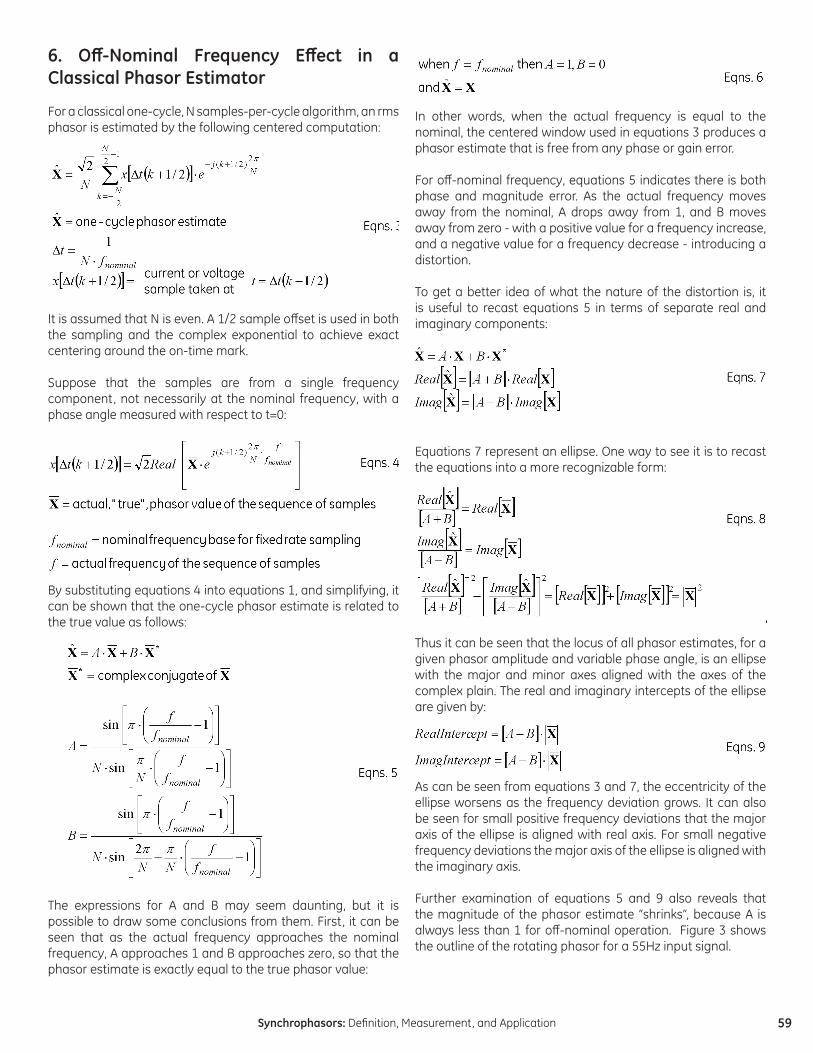
6. Off-Nominal Frequency Effect in a Classical Phasor Estimator

For a classical one-cycle, N samples-per-cycle algorithm, an rms phasor is estimated by the following centered computation:

It is assumed that N is even. A 1/2 sample offset is used in both the sampling and the complex exponential to achieve exact centering around the on-time mark.

Suppose that the samples are from a single frequency component, not necessarily at the nominal frequency, with a phase angle measured with respect to t=0:

By substituting equations 4 into equations 1, and simplifying, it can be shown that the one-cycle phasor estimate is related to the true value as follows:

The expressions for A and B may seem daunting, but it is possible to draw some conclusions from them. First, it can be seen that as the actual frequency approaches the nominal frequency, A approaches 1 and B approaches zero, so that the phasor estimate is exactly equal to the true phasor value:

In other words, when the actual frequency is equal to the nominal, the centered window used in equations 3 produces a phasor estimate that is free from any phase or gain error.

For off-nominal frequency, equations 5 indicates there is both phase and magnitude error. As the actual frequency moves away from the nominal, A drops away from 1, and B moves away from zero - with a positive value for a frequency increase, and a negative value for a frequency decrease - introducing a distortion.

To get a better idea of what the nature of the distortion is, it is useful to recast equations 5 in terms of separate real and imaginary components:

Equations 7 represent an ellipse. One way to see it is to recast the equations into a more recognizable form:

Thus it can be seen that the locus of all phasor estimates, for a given phasor amplitude and variable phase angle, is an ellipse with the major and minor axes aligned with the axes of the complex plain. The real and imaginary intercepts of the ellipse are given by:

As can be seen from equations 3 and 7, the eccentricity of the ellipse worsens as the frequency deviation grows. It can also be seen for small positive frequency deviations that the major axis of the ellipse is aligned with real axis. For small negative frequency deviations the major axis of the ellipse is aligned with the imaginary axis.

Further examination of equations 5 and 9 also reveals that the magnitude of the phasor estimate “shrinks”, because A is always less than 1 for off-nominal operation. Figure 3 shows the outline of the rotating phasor for a 55Hz input signal.

60 Synchrophasors: Definition, Measurement, and Application

7. Out-of-Band interfering signals

Out-of-band signals are those signals occurring on the power system that typically fall in the 0 to 60 Hz range, but specifically those signals that will be aliased if the reporting phasor data rate is too slow for the phenomena being observed. For example, a typical power system swing will operate in the 1 to 3 Hz range.

In order to “observe” a 3 Hz signal, the phasor reporting rate must be greater than twice the 3 Hz swing frequency or 10 phasors per second (the lowest proposed standard rate). More specifically, if there is an interfering signal of 10 Hz with 10% magnitude modulation on the AC waveform (see Figures 4A and 4B for examples) and the reporting rate on the PMU is still set for 10 phasors/second, the proposed standard specifies that influence from the interfering signal shall not raise the TVE above the 1% level.

8. System Architecture

As the implementation of phasor measurement proliferates around the world, there are a number of architectural considerations that need to be addressed. First is physical location. It should be noted that, given PMUs with synchronized current measurement capability, complete observability could be obtained by locating PMUs at alternate nodes in the power system grid.

Current flows from a substation could be used to estimate the voltage at remote stations by calculating the I1*Z1 voltage drop along the line. In general, it is expected that these values will be correlated through a process equivalent to existing state estimators – only 20 times faster.

The next architectural issues to address are those of communications channels and bandwidth. Bandwidth is driven by the user’s appetite for data. For example, choosing a phasor reporting rate of 60 phasors/sec for a voltage, 5 currents, 5 Watt measurements, 5 Var measurements, frequency, and rate of change of frequency – all reporting as floating point

values – will require a bandwidth of 64,000 bps. On the other hand, a data reporting rate of 12 phasors/second for 1 voltage, 5 currents, and frequency – reported in 16 bit integer format – can be accommodated over a 4800 bps channel.

In making the choice of channel bandwidth, both present and future requirements should be considered. In particular, the possibility of future closed loop control should be considered in as much as the speed of this control is a function of the available bandwidth.

Fig 3.Classic Fourier Response for 55Hz Input

Fig 4A.10 Hz Multiplicative Interfering Signal

Fig 4B.10 Hz Additive Interfering Signal

61Synchrophasors: Definition, Measurement, and Application

The next architectural choice is that of a physical communication channel. This choice is driven by several functional requirements, namely:

• Bandwidth required• System availability requirements• Data availability (i.e. – how many lost packets are tolerable)• End-user data distribution

These requirements drive a topological architecture as shown in Figure 5.

In this architecture, there are several data paths shown each of which will require a different data pipe size and characteristic, and there are multiple collection and decision levels that address different operational constraints – the most important being that of speed of response in the case where closed-loop control is involved.

The first line data path is the one from the PMU to a first level Phasor Data Concentrator (PDC) where the data is received and sorted by time-tag from multiple PMUs. Choices for this link include serial data operating with data rates from 9600 bps to 57,600 bps and Ethernet operating at either 10 or 100 MB. Note

that the Synchrophasor standard specifies the data format for the PMU to PDC data link. In many cases, communication redundancy may be required or multiple consumers of data may exist.If serial data links are used, either multiple output ports from the PMU must be supported or a multi-drop serial link must be employed. When supporting multiple consumers through Ethernet, either multiple connections must be supported by the PMU or the PMU can support multicast data transmission.

A particularly useful Ethernet construct that facilitates point-to-multi-point communications is that of the Virtual LAN or VLAN. The VLAN construct adds a 12 bit VLAN identifier to every Ethernet data packet. Ethernet switches that support VLAN can read the VLAN tag and switch the data packet to all ports connected on the same VLAN. Since the switching is done at the data link layer, there is a minimum time delay in switching this data through a network.

Data sharing between PDCs at the same hierarchical level, as well as aggregation PDCs at higher levels, will be required. It is expected, however, that data exchange between PDCs will take place at lower data rates of about 10 synchrophasors/second. Although the data rate is 6 times slower (60 vs. 10 phasors per second), aggregated data streams may contain data from 16 to 32 PMUs. For these aggregated data streams, communication transports such as T1, SONET, and Ethernet should be considered.

One other area to address architecturally is that of data exchange between the PDC and the application software. Inasmuch as the application SW will most likely be multi-vendor, architectural guidelines suggest that a standard generic interface would best serve the industry. The recently released IntelliGrid Architecture4 addresses this issue and recommends the Generic Interface Definition (GID) High Speed Data Access interface for this application. In a practical implementation, this is implemented via the OLE for Process Control standard (OPC). An implementation of this PDC architecture is shown in Figure 6.

Fig 6.Phasor Data Concentrator Architecture

Fig 5.Synchrophasors Data Collection Topology

62 Synchrophasors: Definition, Measurement, and Application

9. Applications

The utility industry has taken a 2-phase approach to the development of applications in the synchrophasor domain. Phase 1 (where most of the world is presently operating) is a data visualization stage / problem identification phase. Visualization tools have been developed that look at dynamic power flow, dynamic phase angle separation, and real-time frequency as well as rate of change of frequency displays. Figure 7 is an example of a real-time plot of the voltage phasor. The contour of the surface indicates instantaneous voltage magnitude and the color indicates phase angle with respect to a user-chosen reference angle. At a glance, any depression indicates a Var sync and the color variation (blue to red) indicates instantaneous power flow. In a control room, this graphic could be animated to show undulations in real time due to power swings.

Other visualization tools that have been developed include a synchroscope view of all the phase angles, frequency and rate of change of frequency plots, oscillation frequency and damping coefficient plots, and general power flow plots.

Phase 2 involves development of a phasor based closed loop control system (Figure 8). In such a system, aggregated measurements from one or more PDCs is passed to a “decision algorithm” that computes, in real-time, a control strategy and issues the appropriate outputs to the controllable devices located around the system. Control speeds will need to vary, based on the severity of the disturbance. If a potentially unstable power swing is detected, the controller has between ¼ and ½ second to compute and initiate a control action.

On the other hand, if the function being implemented is a system-wide automatic Voltage control algorithm, then a control in the multiple-second range is quite adequate. Other potential control algorithms include inter-area oscillation damping, enhanced power system stabilization, automatic voltage regulation, out-of-step tripping and blocking, and voltage collapse detection and mitigation.

Fig 7.Wide Area Voltage View Example

Fig 8.Closed Loop Power System Control

10. Conclusions

The technology and necessary standards for the measurement and communication of synchronized phasor measurements are becoming available across a range of operating platforms. The need of, and potential applications for, this technology are evolving in parallel; the technology will be called upon to maintain stable operation of the electric power grid of the future.

11. References

[1] Complex Quantities and their use in Electrical Engineering; Charles Proteus Steinmetz; Proceedings of the International Electrical Congress, Chicago, IL; AIEE Proceedings, 1893; pp 33-74.

[2] A New Measurement Technique for Tracking Voltage Phasor, Local System Frequency, and Rate of Change of Frequency; A. Phadke, J. Thorp, M. Adamiak; IEEE Trans. vol. PAS-102 no. 5, May 1983, pp 1025-1038

[3] IEEE Standard for Synchrophasors for Power Systems; IEEE 1344 – 1995.

[4] IntelliGrid Architecture (formerly the Integrated Energy and Communication System Architecture; www.e2i.org.