ARTICLE OPEN

Synchronization and causality across time scales in El NiñoSouthern OscillationNikola Jajcay 1,2, Sergey Kravtsov 3,4, George Sugihara5, Anastasios A. Tsonis3,6 and Milan Paluš 1

Statistical inference of causal interactions and synchronization between dynamical phenomena evolving on different temporalscales is of vital importance for better understanding and prediction of natural complex systems such as the Earth’s climate. Thisarticle introduces and applies information theory diagnostics to phase and amplitude time series of different oscillatorycomponents of observed data that characterizes El Niño/Southern Oscillation. A suite of significant interactions between processesoperating on different time scales is detected and shown to be important for emergence of extreme events. The mechanisms ofthese nonlinear interactions are further studied in conceptual low-order and state-of-the-art dynamical, as well as statistical climatemodels. Observed and simulated interactions exhibit substantial discrepancies, whose understanding may be the key to animproved prediction of ENSO. Moreover, the statistical framework applied here is suitable for inference of cross-scale interactions inhuman brain dynamics and other complex systems.

npj Climate and Atmospheric Science (2018) 1:33 ; doi:10.1038/s41612-018-0043-7

INTRODUCTIONA better understanding of dynamics in complex systems, such asthe Earth’s climate or human brain, is one of the key challenges forcontemporary science and society. A large amount of experi-mental data requires new mathematical and computationalapproaches. Natural complex systems vary on many temporaland spatial scales, often exhibiting recurring patterns and quasi-oscillatory phenomena. Data-driven approaches to detection andrecognition of relationships between subsystems in complexsystems have recently become an area of active study in a rangeof scientific fields. For example, thinking about the climate systemas of a complex network of interacting subsystems1 presents anew paradigm that brings out new data analysis methods helpingto detect, describe and predict atmospheric phenomena.2 Acrucial step in constructing climate networks is the inference ofnetwork links between climate subsystems.3 Directed causal linksdetermine which subsystems influence other subsystems, andtheir identification would thus uncover the drivers of atmosphericphenomena. A succinct formalized description of causal relation-ships and synchronizations in complex systems could significantlyimprove our understanding of such systems, which would in turnpromote the development of better schemes to predict theirevolution. Here, we investigate complex, multiple time-scaleinteractions in the El Niño/Southern Oscillation system in theequatorial Pacific.El Niño/Southern Oscillation (ENSO hereafter) is a well known

coupled ocean–atmosphere phenomenon, which manifests as aquasi-periodic fluctuation in sea-surface temperature (El Niño) andair pressure of the overlying atmosphere (Southern Oscillation)across the equatorial Pacific Ocean. It is comprised of two phases,

with the warm phase, known as El Niño, being accompanied by ahigh surface pressure, and the cool phase, La Niña, beingaccompanied by a low surface pressure in the tropical westernPacific. Although the exact causes for initiating warm or cool ENSOevents are not fully understood, the two components of ENSO—sea-surface temperature and atmospheric pressure—are stronglyrelated. ENSO is one of the dominant contributors to the world’sinterannual climate variability.4 Furthermore, strong ENSO eventsexert a large influence on the global atmospheric circulation5 viaassociated teleconnections,6 thus leading to significant socio-economic impacts. An important aspect of ENSO extreme events isthat their positive phase, El Niño, exhibits larger magnitude thantheir negative phase, La Niña.7,8 This suggests that, at least tosome extent, ENSO dynamics involve nonlinear processes.4,9

ENSO events occur irregularly, with a 2–7 year span betweenthem, but have a well defined spatial pattern and seasonaldependence, with the start of development in boreal summer anda peak in boreal winter.10 The individual events generally evolveon a time scale of about two years.5,11 The mechanisms for thisbiennial variability of ENSO are not fully understood either,although it was previously suggested that it is due to year-to-yearalternations between “weak” and “strong” annual cycles in theIndian ocean and western Pacific sector,12 with possible globalrepercussions.13 While the total energy associated with thebiennial component of ENSO signal is not that large comparedwith the background variability, advanced spectral analyses ofvarious ENSO indices14 do identify distinctive quasi-quadriennialand quasi-biennial signals in the equatorial Pacific. In summary,ENSO is known to centrally involve processes on three distincttime scales, namely the ones associated with the annual cycle

Received: 13 February 2018 Revised: 7 August 2018 Accepted: 14 August 2018

1Department of Complex Systems, Institute of Computer Science, Czech Academy of Sciences, Pod Vodárenskou věží 271/2, 182 07 Prague 8, Czech Republic; 2Department ofAtmospheric Physics, Faculty of Mathematics and Physics, Charles University, V Holešovičkách 747/2, 180 00 Prague 8, Czech Republic; 3Department of Mathematical Sciences,Atmospheric Sciences Group, University of Wisconsin-Milwaukee, 3200 N Cramer Street, Milwaukee, WI 53211, USA; 4P. P. Shirshov Institute of Oceanology, Russian Academy ofSciences, Nakhimovskiy Prospekt 36, Moscow 117218, Russia; 5Scripps Institution of Oceanography, University of California San Diego, 8622 Kennel Way, La Jolla, CA 92037, USAand 6Hydrologic Research Center, 11440 West Bernardo Court Suite 375, San Diego, CA 92127, USACorrespondence: Milan Paluš (mp@cs.cas.cz)

www.nature.com/npjclimatsci

Published in partnership with CECCR at King Abdulaziz University

(AC), quasi-biennial (QB) processes, and low-frequency (LF)interannual processes.15–17

Statistical inference of causal relationships within climate datahas recently become an area of active research.18–21 Typically, acausal relation is sought between pairs of different variables ordifferent modes of atmospheric variability. By contrast, Paluš22,23

suggested an approach—which we will follow in the presentstudy—to examine the complexity of climatic interactions byidentifying causal relations between processes operating ondifferent time scales within a single climatic time series. In thisstudy, we apply this technique (see Methods) to discern multi-scale interactions and causality in ENSO, as represented by theNINO3.4 index (spatial average of sea-surface temperatures over abox of 5°S–5°N and 170°–120°W), in observations and climatemodel simulations. Our results uncover intricate causal relation-ships between AC, QB, and LF components of ENSO, and point toa much larger than previously implied role of QB variability inENSO dynamics.

RESULTSInteractions in the observed ENSOWe examined synchronization and causal interactions in theNINO3.4 time series for the quasi-oscillatory modes with periodsranging from 5 to 96 months. We are looking for the observedinteractions characterized by causality estimate exceeding the95th percentile of the distribution of this quantity for thesurrogate data samples (Fig. 1), where the surrogate time serieswere generated using a Monte Carlo method,24 yielding synthetictime series with the same spectrum, but void of any cross-scaleinteractions (see Methods for further details).There are three pairs of modes that exhibit phase synchroniza-

tion (a process by which two or more cyclic signals tend tooscillate with a repeating sequence of relative phase angles) (Fig.1a). The quasi-biennial (QB) modes (periods of 1.8–2.1 year), whichtend to peak in winter (not shown), are indeed synchronized withthe annual cycle (AC) as well as with the so-called combinationtones (CT; periods approximately 9 and 14 months). Thecombination tones result from the interaction of AC with low-frequency (LF) ENSO modes of periods 4–6 yr (see, for example,Stein et al.25 or Stuecker et al.26). Furthermore, the AC and CTmodes with periods of 8–9 months are themselves phase locked.Finally, the LF modes with periods 5–6 yr and QB modes with

periods 2–3 year also exhibit phase synchronization. These resultsreconfirm an important role of the annual cycle in ENSO dynamics,with strong ENSO events peaking in boreal winter,10,27 and pointto the link between QB and LF modes, which may be responsiblefor extreme ENSO events14–16 (see below); thus, our synchroniza-tion analysis brings out known ENSO properties consistent withprevious research.On the other hand, the phase–phase causality diagnostics (Fig.

1b) provides an additional—this time new—information thatcomplements the phase synchronization results and addresses thecauses of these synchronizations by elucidating importantdirected connections between the LF, QB, and AC/CT ENSOmodes. This analysis identifies a member of the pair of modes(time series) that is a skillful precursor of the other member inpredictive context. For example, the phase of LF modes affectsthat of the AC/CT modes, which means that the “shape” of theannual cycle depends on whether the LF mode (periods of4–6 year) is in its extreme warm or extreme cold phase.Furthermore, the phase of the AC mode is a skillful precursor for

the phase of QB modes with the periods of 1.8–2.1 year, while thephase of QB modes with the periods of 2–3-year dictates in partthe phase of the CT modes (periods of 12–16 months).The only pronounced phase–amplitude causality link (Fig. 1c) is

the one between the phase of the LF ENSO mode (periods of5–6 year) and the amplitude of QB modes (periods of 1.8–2.1 year).Our analysis thus identifies the three fundamental time scales in

ENSO dynamics—AC, QB, and LF—consistent with previouswork,15–17 but offers further details on the interaction betweenthese modes. Some of the interactions we identified rigorouslyhere have been previously theorized to exist, but, to the best ofour knowledge, were never detected in a data-driven way. Basedon our results, it is natural to consider the AC and CT processes incombination to define the quasi-annual (QA) variability. The QBmodes can be divided into two—‘‘faster’’ and ‘‘slower’’—sub-ranges, with the periods of 1.8–2.1 year and 2–3 year, respectively.Similarly, the LF processes can be divided into the ones associatedwith 4–5-year and 5–6-year periods.We observe a pronounced connection between the (phase of)

the slower LF mode and both the phase and amplitude of thefaster QB mode. In particular, the slower LF mode affects thephase of the QA mode, and, therefore—indirectly—the phase ofthe faster QB mode, which tends to be affected by and phase-synchronized with the QA mode; the slow LF mode also directlyaffects the amplitude of the faster QB mode. The connections

a b c

Fig. 1 Cross-scale phase synchronization (a), phase–phase causality (b), and phase–amplitude causality (c) in the observed NINO3.4 timeseries. The phase synchronization is a symmetrical relation, hence the plot is symmetric, while causality plots are shown with the period of thedriver (master) time series on the x-axis and driven (slave) time series on the y-axis. Shown are (positive) significance-level deviations from the95th percentile of the k-nearest neighbor estimates of (conditional) mutual information, tested using 500 Fourier transform surrogates (seeMethods)

Synchronization and causality across time scales in El Niño. . .N Jajcay et al.

2

npj Climate and Atmospheric Science (2018) 33 Published in partnership with CECCR at King Abdulaziz University

1234567890():,;

between the phase of slow LF mode and the phase of QA modeimportant in the causal sequence above are both direct andindirect. In the latter indirect case, the connection works throughthe phase synchronization between the slow LF mode and theslow QB mode and subsequent causal effect of the latter on thephase of the QA mode. The faster LF modes add to the picture byalso affecting the phase of the QA mode, and, therefore, indirectly,the phase of the faster QB mode.

Consequences of causal connectionsOne of the main findings of our study is the apparent importance,in ENSO dynamics, of the LF phase→QA phase→QB phasecausal linkages, as well as LF phase→QB amplitude causallinkages. To illustrate these causal connections further, we utilizedan approach of conditional composites, in which we first identifiedthree distinct phases (by dividing the span between maximumand minimum values into three bins) of the low-frequency (LF)ENSO component: LF−, LF0 and LF+; and subsequently computedthe composites (mean values) of any variable of interest over thedata points associated with these three phases.Figure 2 visualizes the response of the AC frequency to changes

in the phase of the LF ENSO variability, thus illustrating the LFphase→QA phase causal linkage. Here, we composited theinstantaneous frequencies of the annual cycle computed as theslope of the continuous 12-month-long snippets of the AC-phasetime series via the robust regression. These results are presentedin the form of histograms and suggest that the positive phase ofthe LF cycle speeds up the annual cycle (thus shortens its periodand increases its frequency), while the negative period of LF cyclecauses the AC period to become longer than a year. Notsurprisingly, the annual cycles associated with neutral LF0conditions, as well as climatological annual cycles, have theaverage period of exactly 1 year.In fact, not only the effective frequency, but also the entire

shape of the annual cycle changes depending on the phase of theLF ENSO mode. Figure 3 shows conditional composites of the

annual cycle associated with the LF−, LF0, and LF+ phases of thelow-frequency ENSO cycle; these composites were computed byaveraging the raw NINO3.4 data associated with a given phase ofLF variability for each month. The neutral LF conditionscorrespond with the seasonal cycle of NINO3.4 temperatures thatis close to climatological seasonal cycle. The latter cycle is notpurely harmonic, and is characterized by relatively fast warmingbetween January and May and a slower cooling afterwards. Theannual cycle conditioned on LF− phase has the same generalcharacter, but is on average colder than the climatological AC. Theannual cycle associated with the LF+ phase of interannual ENSOsignal is, of course, warmer on average due to El Niño-typeconditions, but also has a very different, more harmonic shape,with September-through-December warming absent from the LF−, LF0, and climatological annual cycles. Also shown in Fig. 3 arethe NINO3.4 time series during two extreme El Niño events(namely, 1982/83 and 1997/98 events). Note how a very strongbiennial ENSO signal during those years completely masks anyvisible AC variability that may be present in the NINO3.4 timeseries at that time. An episodic character of such pronouncedbiennial extreme events makes it difficult to associate the QBENSO variability with alterations between weak and strong annualcycles, as was suggested previously.12 We argued that suchextreme ENSO events arise due to synchronization between asuite of different QB modes, which are individually characterizedby a relatively small variance.We hypothesize here that these ‘‘internal’’ QB synchronizations

arise due to causal interactions represented by the QA phase→QB phase causal linkage identified by our conditional mutualinformation analysis. This linkage is further illustrated, albeitindirectly, in Fig. S2 in the Supplementary Material, which showsthat the composite annual cycles associated with QB–, QB0, andQB+ phases of QB variability closely match those associated withLF−, LF0, and LF+ phases, respectively, consistent with LFphase→QA phase→QB phase-directed connections.

Fig. 2 Histograms of instantaneous frequencies of the NINO3.4 annual cycle. Top: unconditioned (using all data); bottom: histogramsconditioned on the phase of the low-frequency (LF) ENSO mode. The black horizontal line marks exactly 1 year period, and also given arerespective means ± one standard deviation of instantaneous frequencies for all four panels

Synchronization and causality across time scales in El Niño. . .N Jajcay et al.

3

Published in partnership with CECCR at King Abdulaziz University npj Climate and Atmospheric Science (2018) 33

Moreover, Fig. S3 in the Supplementary Material identifies cleargrowth in the amplitude of the BC and QB variability as the low-frequency phase changes from La Niña (LF−) to El Niño (LF+)conditions, consistent with the LF phase→QB amplitude causalinteraction. On the other hand, the changes in the amplitude ofAC conditioned on the LF phases are non-monotonic andsomewhat less pronounced compared to those in BC and QBamplitudes.The interactions identified above are instrumental in setting up

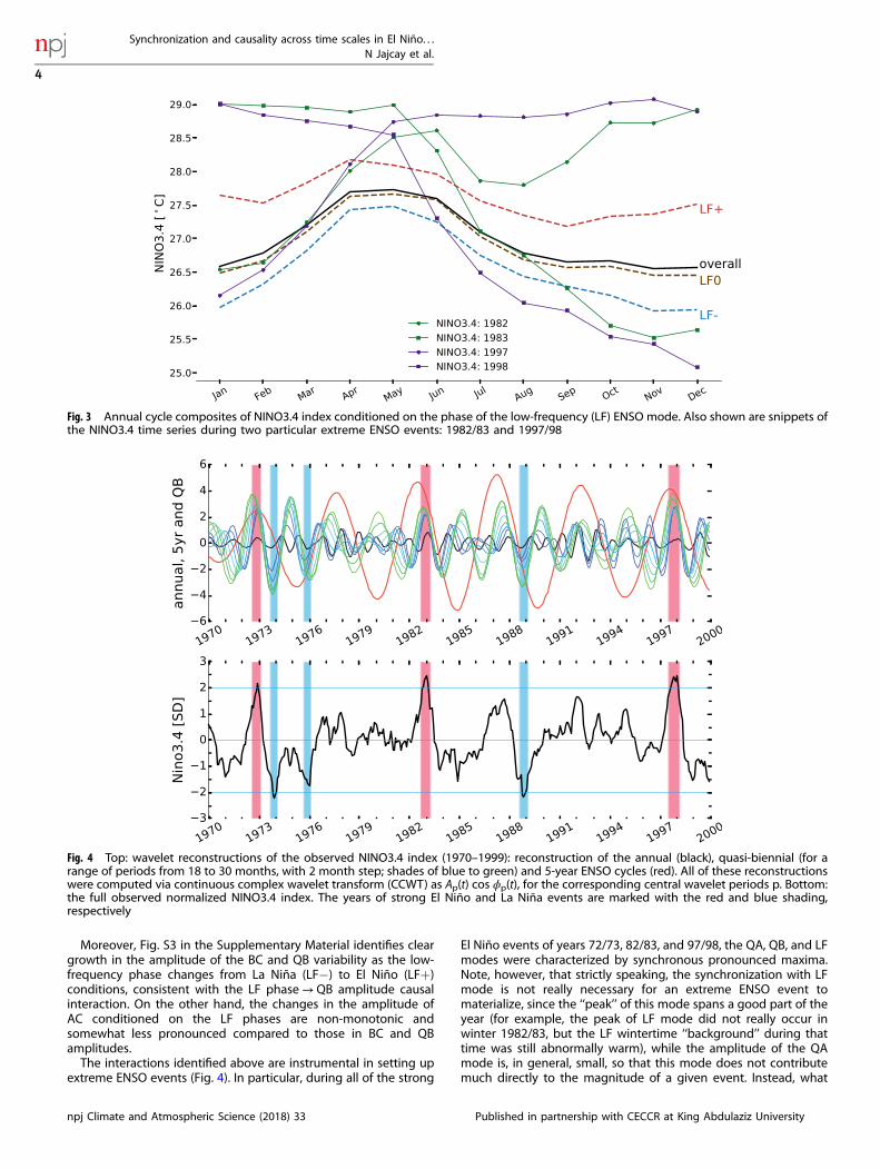
extreme ENSO events (Fig. 4). In particular, during all of the strong

El Niño events of years 72/73, 82/83, and 97/98, the QA, QB, and LFmodes were characterized by synchronous pronounced maxima.Note, however, that strictly speaking, the synchronization with LFmode is not really necessary for an extreme ENSO event tomaterialize, since the ‘‘peak’’ of this mode spans a good part of theyear (for example, the peak of LF mode did not really occur inwinter 1982/83, but the LF wintertime ‘‘background’’ during thattime was still abnormally warm), while the amplitude of the QAmode is, in general, small, so that this mode does not contributemuch directly to the magnitude of a given event. Instead, what

Fig. 3 Annual cycle composites of NINO3.4 index conditioned on the phase of the low-frequency (LF) ENSO mode. Also shown are snippets ofthe NINO3.4 time series during two particular extreme ENSO events: 1982/83 and 1997/98

Fig. 4 Top: wavelet reconstructions of the observed NINO3.4 index (1970–1999): reconstruction of the annual (black), quasi-biennial (for arange of periods from 18 to 30 months, with 2 month step; shades of blue to green) and 5-year ENSO cycles (red). All of these reconstructionswere computed via continuous complex wavelet transform (CCWT) as Ap(t) cos ϕp(t), for the corresponding central wavelet periods p. Bottom:the full observed normalized NINO3.4 index. The years of strong El Niño and La Niña events are marked with the red and blue shading,respectively

Synchronization and causality across time scales in El Niño. . .N Jajcay et al.

4

npj Climate and Atmospheric Science (2018) 33 Published in partnership with CECCR at King Abdulaziz University

appears to be essential for an extreme ENSO to occur is thesynchronization of multiple QB modes with each other. We believethat this ‘‘internal’’ QB synchronization is what has been picked upby our conditional mutual information analysis in the form ofLF→QA→QB phase connections and also LF phase→QBamplitude connections (since synchronization of phases ofdifferent QB modes should automatically result in a large-amplitude event.) By contrast, during a moderate El Niño of 87/88, the LF, QB, and QA modes exhibited phase shifts, with lower-frequency modes leading the higher-frequency modes (inparticular a suite of QB modes) instead of being ‘‘stacked’’ ontop of one another, thus limiting the magnitude of this event.Notably, strong La Niña events do not seem to be associated withthe minimum of the LF mode, but instead occur during near-neutral LF conditions when the minima of the QA modes and theminima of the whole range of QB modes synchronize. Thus, inboth El Niño and La Niña cases, the behavior of the QB modes hasa vital control on the magnitude of the ENSO events.

Interactions in CMIP5 modelsThe Coupled Model Intercomparison Project Phase 5 (CMIP5)28 is aframework for coordinated climate change experiments providingglobal circulation model (GCM) outputs from various modelinggroups. We analyzed time series of the sea-surface temperatureobtained from the individual runs of CMIP5 models and comparedthe simulated NINO3.4 characteristics with the observed char-acteristics (Fig. 5). To start with, we measured the similaritybetween the observed and simulated wavelet spectra29 usingroot-mean-square distance and Pearson correlation coefficient,with zero distance and unit correlation coefficient indicating theperfect match. The ensemble-mean values of these two measuresfor individual CMIP5 models are shown in the first two columns ofFig. 5. The models exhibit great variations in their ability to matchthe observed NINO3.4 spectra, with correlation coefficientsranging from 0.2 to 0.8 and rms distances from 30 to 120;furthermore, there are also substantial sampling variations in theNINO3.4 spectra from multiple runs of a single model (not shown).This means that the ENSO tends to exhibit different epochs ofsampling variability in models, in which its strength, spectrum andother properties may vary significantly.30

Similarly to the wavelet spectra, the synchronization andcausality maps (see examples in Fig. 6 analogous to the observedmaps of Fig. 1), vary considerably from model to model (Fig. 5,right columns), as well as between individual runs of a singlemodel (see Supplementary Excel Table). We compared theobserved and simulated maps using, once again, the standardPearson correlation coefficient, as well as the so-called AdjustedRand Index (ARI), which is especially well suited to measure thesimilarity of clustered data.31 Both measures were computed forthe pairs of interaction maps (observation vs. individual simula-tion) filled with ones or zeros depending on whether thesignificant interaction between the processes of different timescales was identified or not (so the colored areas of maps in Figs. 1and 6 would be filled with ones, and white areas—with zeros);hereafter, we will call the maps so constructed the thresholdedbinary maps.The above similarity measures averaged over the ensembles of

individual model simulations (Fig. 5, right columns) are in factfairly low. For phase synchronization, the highest similarity wasdetected in the CanESM2 model, at the 0.24 level. The phasesynchronization map for the best run of the CanESM2 model (Fig.6a) indicates synchronization between the processes with thesame time scales as in the observed data (Fig. 1a), that is, betweenthe LF, QB, and AC/CT modes. This, however, is more of anexception than a rule, as the time scales of significant phasesynchronization in most of the runs do not match the observedtime scales.

The similarity levels between phase–phase causality maps fromobservations and model simulations are about the same as forphase synchronization maps, with maximum ensemble-meancorrelation of 0.23 obtained for the CCSM4 model. The causalitymap for the best run of this model (Fig. 6b) is correlated with theobserved map (Fig. 1b) at the 0.41 level, and captures correctly theobserved LF–QA, LF–QB, and QA–QB connections. Note that thebest matches to the observed maps in terms of phasesynchronization and phase–phase causality come from individualsimulations of different models, meaning that neither model runwas able to capture the entirety of the observed interactions.Finally, no model was able to capture the observedphase–amplitude causal connection between the LF and QBmodes (Fig. 1c). The highest ensemble-mean correlation betweenthe observed and simulated maps is only 0.03 (MRI-CGCM3), withthe highest correlation of 0.1 for one of the CSIRO-mk360simulations (the corresponding causality map is shown in Fig.6c). The phase-synchronization and phase–phase causality mapsfor the latter run are, however, inferior to those from other modelsin terms of their similarity to the observed maps (not shown).To summarize, the CMIP5 models exhibit great sampling

variations in the simulated ENSO characteristics. Some of thesimulations do exhibit certain aspects of interactions between theprocesses of different time scales, which match the observedinteractions. However, no single simulation is able to reproducethe entire sequence of causal connections inferred from theobserved data.

Fig. 5 Measures of similarity between various characteristics of theobserved and CMIP5 simulated NINO3.4 time series. Shown areensemble averages of these characteristics over multiple runs ofindividual models (see the model acronyms on the left). The first twocolumns compare the observed and simulated wavelet spectra,using the root-mean-square (rms) distance and Pearson correlation,both computed in the frequency space. Next three pairs of columnsdisplay measures of similarity between the observed and simulatedinteraction maps analogous to the observed maps of Fig. 1, namelythe phase synchronization, phase–phase causality andphase–amplitude causality maps. Each pair presents two distinctsimilarity measures: the Pearson correlation (corr) in the phase spaceof the corresponding map, as well as the Adjusted Rand Index (ARI;see text)

Synchronization and causality across time scales in El Niño. . .N Jajcay et al.

5

Published in partnership with CECCR at King Abdulaziz University npj Climate and Atmospheric Science (2018) 33

Interactions in conceptual and statistical modelsThe same interactions were also sought in a conceptual, low-dimensional dynamical model (parametric recharge oscillator:PRO25), as well as in the empirical stochastic (EMR) model of Pacificsea-surface temperatures due to Kondrashov et al.,32 which wereboth used to produce synthetic NINO3.4 time series. The resultsfor both models are presented in the Supplementary Material. In anutshell, the PRO dynamical model fails to reproduce any of theobserved causal interactions (Supplementary Figs. S4 and S5),whereas the EMR statistical model does offer promising results,especially with regards to reproducing the observed LF→QA→QB phase causality (Supplementary Fig. S6). Some of the initialanalyses suggest that the QB modes in the EMR model areinherently present in the algebraic structure of this model’sdeterministic propagator, but are strongly influenced by thefeedbacks that involve state-dependent (multiplicative) noise(Supplementary Fig. S7).

DISCUSSIONIn this study, we examined causal interactions between differentoscillatory modes comprising ENSO variability, using the tools ofinformation theory.22,23 These tools enabled us to uncover anintricate network of interactions underlying the observed ENSOvariability. In particular, we showed that the (phase of) low-frequency (LF), interannual ENSO mode directly affects theamplitude of QB variability. It also indirectly affects the phase ofQB variability, via the intermediate causal connection with thephase of the annual cycle (AC) and its combination tones (CT)associated with the LF mode.33 The AC/CT modes combinedconstitute the quasi-annual (QA) variability (changes in the shapeof the annual cycle). The above LF→QA→QB phase interactionsand LF phase→QB amplitude interactions result in intermittentsynchronizations among different QB modes that occur preferen-tially during certain phases of the LF mode, thus leading toextreme (biennial) ENSO events (Fig. 4). This allows multiple QBmodes, which are normally de-synchronized and are thusassociated with small overall energy, to occasionally produce asignal with the amplitude exceeding those of QA and LF cycles.One of the key messages from our work is to suggest a muchmore important role of the quasi-biennial (QB) modes in ENSOdynamics than, perhaps, thought previously.The three important time scales—QA, QB, and LF—detected by

our independent analysis of ENSO interactions have beenidentified in previous studies as well.15–17 Our results onsynchronization of QB and QA modes are also consistent withprevious work.25,34 However, the novelty of our work, aside from

applying an original methodology to analyze climate data, is inobtaining a new compact description of the causal interactionsinstrumental in ENSO dynamics. The causal connection betweenthe phase of the LF variability and that of the QA variability—thatis, changes in the shape of the annual cycle depending on thestate of the LF ENSO mode—is conceptually similar to the effect oflow-frequency component of North Atlantic Oscillation variabilityon the annual cycle of surface temperature over Europe.35 Amechanistic explanation of the QA→QB phase causality remainselusive, with possible hints from empirical modeling (see below).A growing number of studies identified and analyzed decadal

and longer time scale variability in ENSO.36–42 A major theme inthe studies of decadal ENSO variability is the existence of distinctepochs exhibiting a different character (frequencies, magnitudes,teleconnections) of ENSO and, presumably, distinct dynamicalmechanisms underlying the ENSO variability30,41–45 during theseepochs. It seem likely, therefore, that these dynamics could alterdominant causal interactions in the ENSO system, leading todecadal variations in its cross-scale coupling. In the present work,however, we had to restrict the range of the time scalesconsidered to sub-decadal variability due to a limited length(120 years) of the available ENSO time series, which precludesrobust detection of causal connections on decadal and longertime scales.The observed ENSO interactions are poorly represented in the

historical simulations of CMIP5 climate models, which exhibit largesampling variations in ENSO spectra and causality maps, bothfrom model to model and among different runs of a single model.Some of the model simulations match time scales or selectcausality characteristics of the observed ENSO variability, but nosingle simulation is able to reproduce the full picture of theobserved interactions. The ENSO variability in long pre-industrialcontrol runs of CMIP5-type models is known to exhibit multi-decadal epochs characterized by different ENSO behavior.30

Hence, there is still a possibility that the models possess correctENSO dynamics, but the sample of 89 twentieth-century simula-tions considered here was simply not large enough to generatethe ENSO epoch that would match the observed epoch. Analysesof long pre-industrial runs are needed in order to address thisissue. However, the experiments with an empirical stochasticENSO model of Kondrashov et al.32 suggest that the chances ofreproducing the observed ENSO behavior in ensemble simulationsof the twentieth century climate are much higher than the CMIP5ensemble results. This implies that CMIP5 models do indeedmisrepresent ENSO dynamics. The same conclusion holds for theconceptual parametric recharge oscillator model of Stein et al.,25

which also fails to capture the observed cross-scale causal

a b c

Fig. 6 The same as in Fig. 1, but for the individual simulations of CMIP5 models that best match the observed structures: phasesynchronization in CanESM model (a); phase–phase causality in CCSM4 model (b); and phase–amplitude causality in CSIRO-mk360 model (c)

Synchronization and causality across time scales in El Niño. . .N Jajcay et al.

6

npj Climate and Atmospheric Science (2018) 33 Published in partnership with CECCR at King Abdulaziz University

relationships in ENSO. By contrast, the success of the empiricalENSO model in reproducing the essential phase interactionsamong LF, QA, and QB modes allows one to address, in amechanistic fashion, the dynamics of these interactions, withinitial indications pointing to the importance of both deterministicdynamics and state-dependent (multiplicative) noise in controllingthe QB variability.Thus, neither conceptual nor state-of-the-art dynamical climate

models studied here were able to mimic the structure of theobserved ENSO interactions, while the empirical models consid-ered did quite a bit better. Understanding the discrepanciesbetween the observed interactions and the interactions simulatedby the dynamical models—especially with respect to their abilityto model the QB modes—may be the key to an improved ENSOprediction. On a broader scale, the framework we used here isapplicable to analyzing phenomena across a wide range ofdisciplines—for example, in neuroscience, where cross-frequencyphase–amplitude coupling has recently been observed in electro-physiological signals reflecting the brain dynamics. This cross-frequency coupling enriches the cooperative behavior of neuronalnetworks and apparently plays an important functional role inneuronal computation, communication, and learning.46

METHODSWe analyzed monthly NINO3.4 sea-surface temperature data47 with thetemporal span of 1900–2010, as well as the simulated NINO3.4 time seriesextracted from 89 historic simulations of 15 different global climate models(see Table S1 in Supplementary Material) participating in the CMIP5intercomparison project.28 Both observed and modeled NINO3.4 timeseries were centered to zero mean before entering the analysis.Following Paluš,22,23 we studied interactions between the processes

dominated by different time scales using the phase dynamics approach.48

In particular, we first applied, to the NINO3.4 time series, the complexcontinuous wavelet transform (CCWT) with Morlet mother wavelet29 andobtained time-dependent complex wavelet coefficients ψp(t) for a givencentral period p, from which we extracted the instantaneous phase, ϕp(t),and amplitude, Ap(t), time series. Subsequently, we computed the(conditional) mutual information I49 and applied a randomizationprocedure24 to establish a statistical significance of the results. Themethods are in detail described in the Supplementary Material. TheSupplementary Material moreover discusses possible artefacts of ourmethod and their control and robustness analyses of our results.

DATA AVAILABILITYAll data used in this study are publicly available at the respective sites listed in thereferences. All scripts used in this study are written in Python and are publiclyavailable at the github.com profile of N.J. at https://github.com/jajcayn/enso_cmi.

ACKNOWLEDGEMENTSWe acknowledge the World Climate Research Program’s Working Group on CoupledModeling, which is responsible for CMIP, and we thank the climate modeling groupsfor producing and making available their model output. The U.S. Department ofEnergy’s Program for Climate Model Diagnosis and Intercomparison providescoordinating support for CMIP project and led development of software infra-structure in partnership with the Global Organization for Earth System SciencePortals. Lastly, we would like to thank two anonymous reviewers whose insightfulcomments and questions helped us to strengthen and clarify the manuscript. Thisstudy was supported by the Ministry of Education, Youth and Sports of the CzechRepublic within the Program KONTAKT II, project LH14001 (N.J. and M.P.), by NSFgrants OCE-1243158 (S.K.), AGS-1408897 (S.K. and A.A.T.), DBI-1667584 and DEB-1655203 (G.S.), as well as by the Ministry of Education and Science of the RussianFederation (project #14.W03.31.0006) and Russian Science Foundation (project #14-50-00095) (S.K.), and finally with Lenfest Ocean Program grant 00028335 (G.S.) andDoD–Strategic Environmental Research and Development Program 15 RC-2509 (G.S.).

AUTHOR CONTRIBUTIONSN.J. and M.P. designed the study, N.J. and S.K. prepared the data and carried out theanalysis, S.K. provided the empirical model, N.J. and S.K. prepared the manuscript. Allauthors discussed the results and contributed to editing the manuscript. A.A.T. andM.P. supervised the study.

ADDITIONAL INFORMATIONSupplementary information accompanies the paper on the npj Climate andAtmospheric Science website (https://doi.org/10.1038/s41612-018-0043-7).

Competing interests: The authors declare no competing interests.

Publisher's note: Springer Nature remains neutral with regard to jurisdictional claimsin published maps and institutional affiliations.

REFERENCES1. Tsonis, A. A. & Roebber, P. J. The architecture of the climate network. Phys. A 333,

497–504 (2004).2. Havlin, S. et al. Challenges in network science: Applications to infrastructures,

climate, social systems and economics. Eur. Phys. J. Spec. Top. 214, 273–293(2012).

3. Paluš, M., Hartman, D., Hlinka, J. & Vejmelka, M. Discerning connectivity fromdynamics in climate networks. Nonlinear Proc. Geoph. 18, 751–763 (2011).

4. Neelin, J. D. et al. ENSO theory. J. Geophys. Res. Oceans 103, 14261–14290 (1998).5. Trenberth, K. E. et al. Progress during TOGA in understanding and modeling

global teleconnections associated with tropical sea surface temperatures. J.Geophys. Res. Oceans 103, 14291–14324 (1998).

6. Alexander, M. A. et al. The atmospheric bridge: The inuence of ENSO tele-connections on air-sea interaction over the global oceans. J. Clim. 15, 2205–2231(2002).

7. Burgers, G. & Stephenson, D. B. The normality of El Niño. Geophys. Res. Lett. 26,1027–1039 (1999).

8. Sardeshmukh, P. D., Compo, G. P. & Penland, C. Changes of probability associatedwith El Nino. J. Clim. 13, 4268–4286 (2000).

9. Ghil, M. & Robertson, A. W. Solving problems with GCMs: General circulationmodels and their role in the climate modeling hierarchy. Int. Geophys. 70,285–325 (2001).

10. Larkin, N. K. & Harrison, D. E. ENSO warm (El Niño) and cold (La Niña) event lifecycles: Ocean surface anomaly patterns, their symmetries, asymmetries, andimplications. J. Clim. 15, 1118–1140 (2002).

11. Barnett, T. P. Variations in near-global sea level pressure: Another view. J. Clim. 1,225–230 (1988).

12. Meehl, G. A. The annual cycle and interannual variability in the tropical Pacificand Indian Ocean regions. Mon. Weather Rev. 115, 27–50 (1987).

13. Lau, K. -M. & Sheu, P. J. Annual cycle, quasi-biennial oscillation, and southernoscillation in global precipitation. J. Geophys. Res. Atmos 93, 10975–10988 (1988).

14. Jiang, N., Neelin, J. D. & Ghil, M. Quasi-quadrennial and quasi-biennial variabilityin the equatorial Pacific. Clim. Dynam. 12, 101–112 (1995).

15. Barnett, T. P. The interaction of multiple time scales in the tropical climate system.J. Clim. 4, 269–285 (1991).

16. Kim, K. -Y. Investigation of ENSO variability using cyclostationary EOFs ofobservational data. Meteorol. Atmos. Phys. 81, 149–168 (2002).

17. Yeo, S. -R. & Kim, K. -Y. Global warming, low-frequency variability, and biennialoscillation: an attempt to understand the physical mechanisms driving majorENSO events. Clim. Dynam. 43, 771–786 (2014).

18. Ebert-Uphoff, I. & Deng, Y. Causal discovery for climate research using graphicalmodels. J. Clim. 25, 5648–5665 (2012).

19. Runge, J. et al. Identifying causal gateways and mediators in complex spatio-temporal systems. Nat. Comm. 6, 8502 (2015).

20. van Nes, E. H. et al. Causal feedbacks in climate change. Nat. Clim. Change 5,445–448 (2015).

21. Hannart, A., Pearl, J., Otto, F. E. L., Naveau, P. & Ghil, M. Causal counterfactualtheory for the attribution of weather and climate-related events. B. Am. Meteorol.Soc. 97, 99–110 (2016).

22. Paluš, M. Multiscale atmospheric dynamics: cross-frequency phase-amplitudecoupling in the air temperature. Phys. Rev. Lett. 112, 078702 (2014).

23. Paluš, M. Cross-scale interactions and information transfer. Entropy 16,5263–5289 (2014).

24. Paluš, M. From nonlinearity to causality: statistical testing and inference of phy-sical mechanisms underlying complex dynamics. Conte. Phys. 48, 307–348 (2007).

25. Stein, K., Timmermann, A., Schneider, N., Jin, F. -F. & Stuecker, M. F. ENSO seasonalsynchronization theory. J. Clim. 27, 5285–5310 (2014).

Synchronization and causality across time scales in El Niño. . .N Jajcay et al.

7

Published in partnership with CECCR at King Abdulaziz University npj Climate and Atmospheric Science (2018) 33

26. Stuecker, M. F., Timmermann, A., Jin, F.-F., McGregor, S. & Ren, H. -L. A combi-nation mode of the annual cycle and the El Niño/Southern Oscillation. Nat.Geosci. 6, 540–544 (2013).

27. Torrence, C. & Webster, P. J. The annual cycle of persistence in the El Niño/Southern Oscillation. Q. J. Roy. Meteor. Soc. 124, 1985–2004 (1998).

28. Taylor, K. E., Stouffer, R. J. & Meehl, G. A. An overview of CMIP5 and the experi-ment design. B. Am. Meteorol. Soc. 93, 485 (2012).

29. Torrence, C. & Compo, G. P. A practical guide to wavelet analysis. B. Am. Meteorol.Soc. 79, 61–78 (1998).

30. Wittenberg, A. T. Are historical records sufficient to constrain ENSO simulations?Geophys. Res. Lett. 36(12), L12702 (2009).

31. Hubert, L. & Arabie, P. Comparing partitions. J. Classif. 2, 193–218 (1985).32. Kondrashov, D., Kravtsov, S., Robertson, A. W. & Ghil, M. A hierarchy of data based

ENSO models. J. Clim. 18, 4425–4444 (2005).33. Stuecker, M. F., Jin, F. -F., Timmermann, A. & McGregor, S. Combination Mode

Dynamics of the Anomalous Northwest Pacific Anticyclone. J. Clim. 28,1093–1111 (2015).

34. Rasmusson, E. M., Wang, X. & Ropelewski, C. F. The biennial component of ENSOvariability. J. Mar. Syst. 1, 71–96 (1990).

35. Palus, M., Novotn, D. & Tichavsky, P. Shifts of seasons at the European midlatitudes: Natural fluctuations correlated with the North Atlantic Oscillation.Geophys. Res. Lett. 32, L12805 (2005).

36. Latif, M., Kleeman, R. & Eckert, C. Greenhouse warming, decadal variability, or ElNiño? An attempt to understand the anomalous 1990s. J. Clim. 10, 2221–2239(1997).

37. Gershunov, A. & Barnett, T. P. Interdecadal modulation of ENSO teleconnections.Bull. Am. Meteorol. Soc. 79, 2715–2725 (1998).

38. Wang, X., Wang, D. & Zhou, W. Decadal variability of twentieth-century El Niñoand La Niña occurrence from observations and IPCC AR4 coupled models. Geo-phys. Res. Lett. 36, L11701 (2009).

39. Okumura, Y. M., Sun, T. & Wu, X. Asymmetric modulation of El Niño and La Niñaand the linkage to tropical Pacific decadal variability. J. Clim. 30, 4705–4733(2017).

40. Duan, W. & Mu, M. Investigating decadal variability of El Niño-Southern Oscilla-tion asymmetry by conditional nonlinear optimal perturbation. J. Geophys. Res.Oceans 111, C07015 (2006).

41. Sullivan, A. et al. Robust contribution of decadal anomalies to the frequency ofcentral-Pacific El Niño. Sci. Rep. 6, 38540 (2016).

42. Ruprich-Robert, Y. et al. Assessing the climate impacts of the observed Atlanticmulti decadal variability using the GFDL CM2. 1 and NCAR CESM1 global coupledmodels. J. Clim. 30, 2785–2810 (2017).

43. Vecchi, G. A. & Wittenberg, A. T. El Niño and our future climate: where do westand?. Wires.: Clim. Change 1, 260–270 (2010).

44. Moy, C. M., Seltzer, G. O., Rodbell, D. T. & Anderson, D. M. Variability of El Niño/Southern Oscillation activity at millennial timescales during the Holocene epoch.Nature 420, 162 (2002).

45. Chen, C., Cane, M. A., Wittenberg, A. T. & Chen, D. ENSO in the CMIP5 simulations:life cycles, diversity, and responses to climate change. J. Clim. 30, 775–801 (2017).

46. Canolty, R. T. & Knight, R. T. The functional role of cross-frequency coupling.Trends Cogn. Sci. 14, 506–515 (2010).

47. Rayner, N. A. et al. Global analyses of sea surface temperature, sea ice, and nightmarine air temperature since the late nineteenth century. J. Geophys. Res. Atmos.108, 4407 (2003). Data retrieved from https://www.esrl.noaa.gov/psd/gcos_wgsp/Timeseries/Data/nino34.long.data.

48. Pikovsky, A., Rosenblum, M. & Kurths, J. Synchronization: A UniversalConcept in Nonlinear Sciences, Vol. 12 (Cambridge University Press, Cambridge,UK, 2003).

49. Paluš, M. & Vejmelka, M. Directionality of coupling from bivariate time series:How to avoid false causalities and missed connections. Phys. Rev. E 75, 056211(2007).

Open Access This article is licensed under a Creative CommonsAttribution 4.0 International License, which permits use, sharing,

adaptation, distribution and reproduction in anymedium or format, as long as you giveappropriate credit to the original author(s) and the source, provide a link to the CreativeCommons license, and indicate if changes were made. The images or other third partymaterial in this article are included in the article’s Creative Commons license, unlessindicated otherwise in a credit line to the material. If material is not included in thearticle’s Creative Commons license and your intended use is not permitted by statutoryregulation or exceeds the permitted use, you will need to obtain permission directlyfrom the copyright holder. To view a copy of this license, visit http://creativecommons.org/licenses/by/4.0/.

© The Author(s) 2018

Synchronization and causality across time scales in El Niño. . .N Jajcay et al.

8

npj Climate and Atmospheric Science (2018) 33 Published in partnership with CECCR at King Abdulaziz University