rspa.royalsocietypublishing.org

ResearchCite this article: Xie H-B, Guo T, Sivakumar B,Wee-Chung Liew A, Dokos S. 2014 Symplecticgeometry spectrum analysis of nonlinear timeseries. Proc. R. Soc. A 470: 20140409.http://dx.doi.org/10.1098/rspa.2014.0409

Received: 22 May 2014Accepted: 10 July 2014

Subject Areas:Chaos theory

Keywords:symplectic geometry spectrum analysis,chaotic time series, attractorreconstruction, prediction

Author for correspondence:Hong-Bo Xiee-mail: xiehb@sjtu.org

Symplectic geometryspectrum analysis of nonlineartime seriesHong-Bo Xie1, Tianruo Guo1, Bellie Sivakumar2,3,

Alan Wee-Chung Liew4 and Socrates Dokos1

1Graduate School of Biomedical Engineering, and 2School of Civiland Environmental Engineering, The University of New SouthWales, Sydney, New South Wales 2052, Australia3Department of Land, Air and Water Resources, University ofCalifornia, Davis, CA 95616, USA4School of Information and Communication Technology, GriffithUniversity, Gold Coast, Queensland 4222, Australia

Various time-series decomposition techniques, includ-ing wavelet transform, singular spectrum analysis,empirical mode decomposition and independentcomponent analysis, have been developed for non-linear dynamic system analysis. In this paper, wedescribe a symplectic geometry spectrum analysis(SGSA) method to decompose a time series into aset of independent additive components. SGSA isperformed in four steps: embedding, symplecticQR decomposition, grouping and diagonal aver-aging. The obtained components can be used forde-noising, prediction, control and synchronization.We demonstrate the effectiveness of SGSA inreconstructing and predicting two noisy benchmarknonlinear dynamic systems: the Lorenz and Mackey-Glass attractors. Examples of prediction of adecadal average sunspot number time series anda mechanomyographic signal recorded from humanskeletal muscle further demonstrate the applicabilityof the SGSA method in real-life applications.

1. IntroductionDynamic behaviour of real-world systems can berepresented by measurements along the temporaldimension, i.e. a time series. Such time series are typicallycollected over long periods of time and are usually asource of a large number of interesting behaviours that

2014 The Author(s) Published by the Royal Society. All rights reserved.

on June 14, 2018http://rspa.royalsocietypublishing.org/Downloaded from

2

rspa.royalsocietypublishing.orgProc.R.Soc.A470:20140409

...................................................

the system may have undergone in the past or evolve into in future. The general objectiveof time-series analysis is to obtain the most essential information regarding the evolutionbehaviours of a dynamic system [1–3]. Decomposition of a time series into a set of components isparticularly useful for such purposes, because reconstruction, prediction, phase synchronizationand control of nonlinear dynamic systems can be readily conducted using these components.Over the past few decades, several time-series decomposition methods have been reported andsuccessfully applied to many problems in nonlinear dynamics, including wavelet transform,independent component analysis (ICA), empirical mode decomposition (EMD) and singularspectrum analysis (SSA).

The wavelet transform decomposes a time series into components in various frequency sub-bands or scales with various resolutions [4]. It provides a framework for studying how frequencycontent changes with time and, consequently, for detection and localization of short-durationphenomena in a dynamic system [5–8]. Chandre et al. [5] described a wavelet-based method toextract the ridges in the time–frequency landscape of a trajectory for analysing the phase spacestructures of Hamiltonian systems. In particular, the method is able to detect resonance trappingsand transitions and allows for characterization of the notion of weak and strong chaos. Ozkurt &Savaci [6,8] further applied the wavelet ridges to reconstruct the spiral and double-scroll attractorsof Chua’s circuit in phase space by time delay embedding. Han et al. [7] developed a wavelet softthreshold technique to smooth the noisy chaotic time series generated by a Lorenz system aswell as the observed annual runoff from the Yellow River. Essentially, wavelet analysis is stillconvolutional, and the ‘mother’ wavelet is phenomenon dependent [4]. The lack of orthogonalityand the limitation of finite length for some of the most commonly used ‘mother’ wavelets cancause unwanted leakage between the different frequency modes [4,9].

ICA is an alternative linear decomposition-based method, deriving spatial filters to factorizeobserved time series into a sum of temporally independent and spatially fixed components [10].ICA is a computationally efficient blind source separation technique, widely used in many fieldsof nonlinear analysis. Shang & Shyu [11] successfully extracted a chaotic Duffing oscillator from anoisy Gaussian environment by using a modified ICA. Chen et al. [12] presented a similar work toextract real chaotic signals from a noisy source. They further developed a new scheme to combinetheir improved ICA design with state feedback control to achieve chaos synchronization. Asano &Nakao [13] used ICA components to analyse the complex dynamics of two types of spatio-temporal chaos. For diffusively coupled complex Ginzburg–Landau oscillators, which exhibitsmooth amplitude patterns, ICA was able to extract localized one-humped basis vectors reflectingthe characteristic hole structures of the system. In addition, for non-locally coupled complexGinzburg–Landau oscillators with fractal amplitude patterns, ICA was able to extract localizedbasis vectors with characteristic gap structures. ICA assumes a linear stationary mixing model inwhich the mixing matrix consists of a set of constants independent of the changing structure of thedata over time. However, for many nonlinear systems, this is only true from certain observationpoints or for very short lengths of time [14].

EMD is an emerging novel signal analysis technique able to decompose any time series intoa set of spectrally independent oscillatory modes, known as intrinsic-mode functions. Comparedwith wavelets, EMD has the inherent advantage that the basic decomposition functions aredetermined by the properties of the data itself. That is, EMD decomposes a signal in a naturalway without prior knowledge of the signal of interest embedded in the data series [4,15]. Severalrecent studies have demonstrated that EMD is particularly useful in phase synchronizationanalysis of complex oscillators with several spectral components as well as for non-stationaryoscillator prediction [16–19]. Unfortunately, the EMD lacks a firm theoretical framework andsuffers from drawbacks, such as extrema locations, extrema interpolation, end effects and siftingstopping criterion [20]. Although some studies have attempted to alleviate the aforementionedproblems, the theoretical basis of EMD still needs to be reinforced to achieve more precise andreliable results.

Distinct from the above techniques, SSA uses singular value decomposition (SVD) to reshapea time series into a sum of independent and interpretable components, such as a slowly

on June 14, 2018http://rspa.royalsocietypublishing.org/Downloaded from

3

rspa.royalsocietypublishing.orgProc.R.Soc.A470:20140409

...................................................

varying trend, oscillatory components and noise [3]. It is now a popular tool for detectingtrends in different resolutions, smoothing, extracting seasonality components, finding structurein short time series, detecting chaos, determining noise level (NL) and testing causality [3,21–23].However, SSA is based on SVD, which is by nature a linear technique. Several studies haveindicated that it can lead to misleading results when nonlinear structures are analysed [24–26].

Distinct from Euclidean geometry, symplectic geometry is even-dimensional, dependent ona bilinear antisymmetric non-singular cross product—the symplectic cross product. Symplecticgeometry originated from and is widely used in the study of Hamiltonian dynamic systems[26–30]. It has been rapidly expanded to describe singular differential equations, partialdifferential equations and other dynamic systems [31]. Its applications have expanded fromclassical mechanics to control theory, geometrical optics, thermodynamics, electromagnetic fields,quantum systems and biomechanics. It can also be used to characterize dissipative dynamicalsystems [32,33]. For example, Ivancevic [32] presented a symplectic geometry approach for use indissipative biological systems of human motion.

Several studies have shown that symplectic geometry-based methods are superior to SVD-based techniques in the detection of chaos [26,27], estimation of the embedding dimensionof a nonlinear dynamic system [29] and de-noising nonlinear systems [30]. In this paper, wepresent a method, termed symplectic geometry spectrum analysis (SGSA), which is parallel towavelets, EMD, ICA and SSA, to decompose a time series into the sum of a small number ofindependent and interpretable components. The idea of SGSA originated from the applicationof symplectic geometry to resolve the eigenvalue problem for optimal control [34–36]. The keydifference between SGSA and the former approaches is that SGSA is based on a symplecticQR decomposition in symplectic space. The derived components can be used to resolve manyproblems, such as de-noising, reconstruction of an attractor, nonlinear prediction, extraction ofseasonality components and detection of change-points. In order to illustrate its applicability,we apply SGSA to reconstruct Lorenz and Mackey-Glass attractors from their noisy series, aswell as to assess the prediction performance of SGSA on them. We further predict the decadalaverage sunspot data and a mechanomyographic (MMG) signal collected from human skeletalmuscle by SGSA to test its effectiveness for real systems. Compared with an improved local linearapproximation (ILLA) method, lower normalized mean square error (NMSE) values obtainedfrom SGSA indicate its potential value for practical application in different fields.

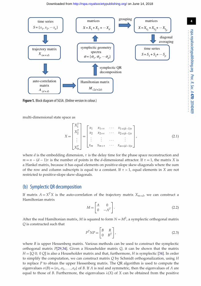
2. Symplectic geometry spectrum analysisThe SGSA method first builds a trajectory matrix from the original time series in a processcalled embedding. This matrix consists of vectors obtained by means of a sliding windowthat traverses the series. The trajectory matrix is transformed into a symmetric form and theninto a Hamiltonian matrix in symplectic space. The Hamiltonian matrix is further subjectedto a symplectic QR decomposition to obtain its eigenvalues and eigenvectors. Each of theseeigenvectors can be transformed into a reconstructed time series, collectively termed symplecticreconstructed components (SRC). The sum of all these SRC is equal to the original time series.Any eigenvectors which negligibly contribute to the norm of the original matrix can be neglected.In order to approximate the original time series, a diagonal averaging technique is applied toevery symplectic principal component matrix. Figure 1 summarizes the block diagram of SGSAtechnique, and the above description may be expressed in formal terms as follows.

(a) EmbeddingConsider a real-valued non-zero time series S = x1, x2, . . . , xn, where n is the number of samples.Takens’ embedding theorem states that a topologically equivalent representation of the originalmulti-dimensional system behaviour can be reconstructed from the one-dimensional signalby means of the method of delay. That is, the original time series can be mapped into a

on June 14, 2018http://rspa.royalsocietypublishing.org/Downloaded from

4

rspa.royalsocietypublishing.orgProc.R.Soc.A470:20140409

...................................................

time series

time seriestrajectory matrix

auto-correlationmatrix

Hamiltonian matrix

matrices

symplectic geometryspectra

matricesgrouping

diagonalaveraging

symplectic QRdecomposition

S = {x1, x2, ... xn}

S = S1 + S2+ ... Sps = {s1, s2, ... sd}

X = X1 + X2 + ... Xd

X (m × d)

A (d × d)M (2d ×2d)

X = XI1+ XI2

+ ... XIp

Figure 1. Block diagram of SGSA. (Online version in colour.)

multi-dimensional state space as

X =

⎡⎢⎢⎢⎢⎢⎢⎣

XT1

XT2

...

XTm

⎤⎥⎥⎥⎥⎥⎥⎦

=

⎡⎢⎢⎢⎢⎣

x1 x1+τ · · · x1+(d−1)τx2 x2+τ · · · x2+(d−1)τ...

... · · ·...

xm xm+τ · · · xm+(d−1)τ

⎤⎥⎥⎥⎥⎦ , (2.1)

where d is the embedding dimension, τ is the delay time for the phase space reconstruction andm = n − (d − 1)τ is the number of points in the d-dimensional attractor. If τ = 1, the matrix X isa Hankel matrix, because it has equal elements on positive-slope skew-diagonals where the sumof the row and column subscripts is equal to a constant. If τ > 1, equal elements in X are notrestricted to positive-slope skew-diagonals.

(b) Symplectic QR decompositionIf matrix A = XTX is the auto-correlation of the trajectory matrix Xm×d, we can construct aHamiltonian matrix

M =[

A 00 −AT

]. (2.2)

After the real Hamiltonian matrix, M is squared to form N = M2, a symplectic orthogonal matrixQ is constructed such that

PTNP =[

B R0 BT

], (2.3)

where B is upper Hessenberg matrix. Various methods can be used to construct the symplecticorthogonal matrix P[29,34]. Given a Householder matrix Q, it can be shown that the matrixH = [Q 0; 0 Q] is also a Householder matrix and that, furthermore, H is symplectic [34]. In orderto simplify the computation, we can construct matrix Q by Schmidt orthogonalization, using Hto replace P to obtain the upper Hessenberg matrix. The QR algorithm is used to compute theeigenvalues σ (B) = {σ1, σ2, . . . , σd} of B. If A is real and symmetric, then the eigenvalues of A areequal to those of B. Furthermore, the eigenvalues λ(X) of X can be obtained from the positive

on June 14, 2018http://rspa.royalsocietypublishing.org/Downloaded from

5

rspa.royalsocietypublishing.orgProc.R.Soc.A470:20140409

...................................................

square roots of σ (B) as

λj = √σj, j = 1, 2, . . . , d, (2.4)

with eigenvalues sorted in descending order

σ1 > σ2 > · · · > σd. (2.5)

The distribution of σj is the symplectic geometry spectra of A with relevant symplecticorthonormal bases. Low values of σj are often related to the noise component in the data. Thecorresponding matrix Q represents the symplectic eigenvectors of A, such that the ith column ofQ (Qi) is equal to the ith eigenvector of A. The transformed coefficients matrix S is then formedsuch that the ith row, Si, is given by

Si = QTi X (i = 1, 2, . . . , d). (2.6)

We then obtain the corresponding reconstructed matrix

Xi = QiSi (i = 1, 2, . . . , d). (2.7)

The trajectory matrix can be written as

X = X1 + X2 + · · · + Xd. (2.8)

(c) GroupingThe purpose of this step is to identify components with different periods as well as the noise.The grouping procedure splits the set of indices (i = 1, 2, . . . , d) into p disjoint subsets I1, I2, . . . , Ip,so that the elementary matrix in equation (2.8) is regrouped into p groups. Let I = {i1, i2, . . . , il},then the resultant matrix corresponding to the group I is defined as XI = Xi1 + Xi2 + · · · + Xil . Thepartition of the set {1, 2, . . . , d} into disjoint subsets I1, I, . . . , Ip corresponds to the new expansion

X = XI1 + XI2 + · · · + XIp . (2.9)

(d) Diagonal averagingThe final step of SGSA is the transformation of each regrouped matrix in equation (2.9) into anew series with the same length n. The aim of diagonal averaging is to generate reconstructedelements of each resultant matrix by averaging over positive-slope skew diagonal groupings.The new element has the same position as the corresponding elements in the original series. Forτ > 1, the diagonal averaging can be carried out using the following algorithm. Consider matrixYm×d with elements yij, 1 ≤ i ≤ m, 1 ≤ j ≤ d. Let d∗ = min(m, d), m∗ = max(m, d) and n = m + (d −1)τ . Let y∗

ij = yij if m < d and y∗ij = yji otherwise. Diagonal averaging transfers matrix Y to a series

y1, y2, . . . , yn according to the following:

yk =

⎧⎪⎪⎪⎪⎪⎪⎪⎪⎪⎪⎪⎪⎪⎨⎪⎪⎪⎪⎪⎪⎪⎪⎪⎪⎪⎪⎪⎩

1k

k∑p=1

y∗p,k−p+1 for 1 ≤ k < d∗

1d∗

d∗∑p=1

y∗p,k−p+1 for d∗ ≤ k ≤ m∗

1n − k + 1

n−m∗+1∑p=k−m∗+1

y∗p,k−p+1 for m∗ < k ≤ n.

(2.10)

Equation (2.10) corresponds to the averaging of the matrix elements over the ‘diagonals’ i + j =k + 1. Such diagonal averaging, applied to any sub-matrix in equation (2.9), generates an n-length

on June 14, 2018http://rspa.royalsocietypublishing.org/Downloaded from

6

rspa.royalsocietypublishing.orgProc.R.Soc.A470:20140409

...................................................

time series, and thus the original series S is decomposed into a sum of p series

S = S1 + S2 + · · · + Sp. (2.11)

For the case τ > 1, we can insert a d∗ × (τ − 1) zero matrix into every two adjacent columns ofYd∗×m∗ to form a new matrix

Y′ =

∣∣∣∣∣∣∣∣∣∣

y11 0 · · · 0 y12 0 · · · 0 y13 · · · y1m∗y21 0 · · · 0 y22 0 · · · 0 y23 · · · y2m∗

... 0 · · · 0... 0 · · · 0

... · · ·...

yd∗1 0 · · · 0 yd∗2 0 · · · 0 yd∗3 · · · yd∗m∗

∣∣∣∣∣∣∣∣∣∣. (2.12)

The diagonal averaging formula (equation (2.10)) is then applied to the new matrix Y′ togenerate the time series. However, the number of elements belonging to every d∗ × (τ − 1) zeromatrix should be subtracted from the total number of diagonal elements when carrying outthe averaging.

With proper choices of d and the sets I1, I2, . . . , Ip, these SRC can be associated with the trend,oscillations or noise of the original time series. If grouping is skipped, the trajectory matrix can bedecomposed into d SRCs.

3. Symplectic geometry spectrum analysis applied to synthetic chaotic dataState space reconstruction and prediction of chaotic time series are two fundamental andimportant problems in chaotic dynamics. To demonstrate the usefulness of the proposed SGSAmethod, we apply it to reconstruct and predict two benchmark chaotic systems embedded innoise: the Lorenz system and the Mackey-Glass system.

The Lorenz system is defined by the following three-state nonlinear ordinary differentialequations:

dxdt

= σ (y − x), (3.1)

dydt

= −xz + rx − y (3.2)

anddzdt

= xy − bz, (3.3)

with parameter values σ = 10, b = 8/3 and r = 28.The Mackey-Glass system is given by the delay differential equation

dxdt

= −bx(t) + ax(t − τ0)1 + xc(t − τ0)

, (3.4)

where a = 0.2, b = 0.1, c = 10 and τ0 = 17.We use fourth-order explicit and implicit Runge–Kutta numerical integration algorithms for

the Lorenz and Glass-Mackey systems, respectively, to simulate the original noise-free timeseries. The integration step for the Lorenz and Mackey-Glass equations were set to 0.02 and 0.5,respectively. The first 5000 points are discarded to eliminate initial transients.

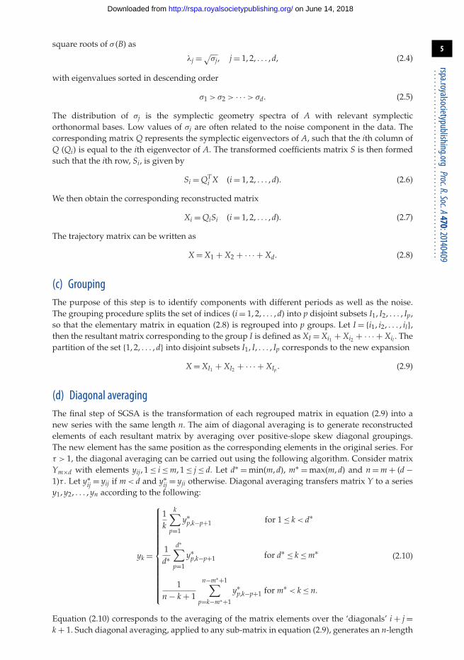
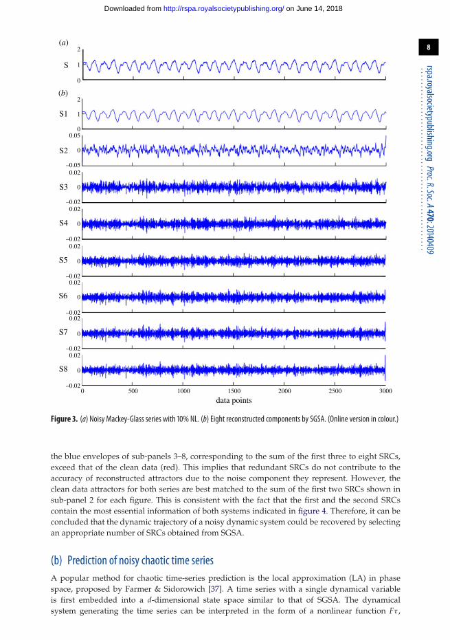
(a) Reconstruction of noisy chaotic attractorsThe embedding dimension for both systems is set to eight. Noise is then superimposed onto thetime series through the addition of independent and identically distributed (i.i.d.) Gaussian whitenoise with various NLs. Figures 2 and 3 illustrate the SGSA decomposition results for the noisyLorenz and Mackey-Glass series, respectively, with 10% NL. The top panel of both figures showsthe original noisy data, whereas the lower panels illustrate the eight reconstructed componentsby SGSA. The first SRC, showing the main trend, is similar to the original series. Compared withthis, the amplitudes of the remaining SRCs are much lower. A simple Fourier transform could

on June 14, 2018http://rspa.royalsocietypublishing.org/Downloaded from

7

rspa.royalsocietypublishing.orgProc.R.Soc.A470:20140409

...................................................

–1

0

1

–0.5

0

0.5

–0.5

0

0.5

–0.5

0

0.5

–0.5

0

0.5

–0.5

0

0.5

0 500 1000 1500 2000 2500 3000–0.5

0

0.5

–20

0

20

–20

0

20

S1

S2

S3

S4

S5

S6

S7

S8

S

(a)

(b)

data points

Figure 2. (a) x component of noisy Lorenz series with 10% NL. (b) Eight reconstructed components by SGSA. (Online version incolour.)

indicate the different frequency band distributions of each SRC. These results demonstrate thatSGSA can reliably extract various sub-band components from the original series, highlightingits ability in various applications, including time-series de-noising, compression, prediction andtrend detection.

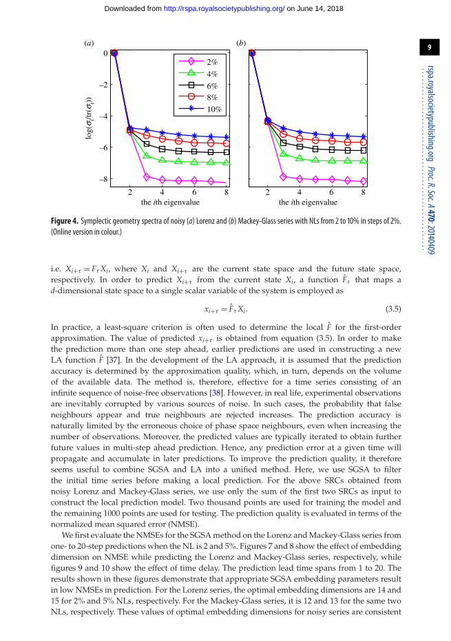
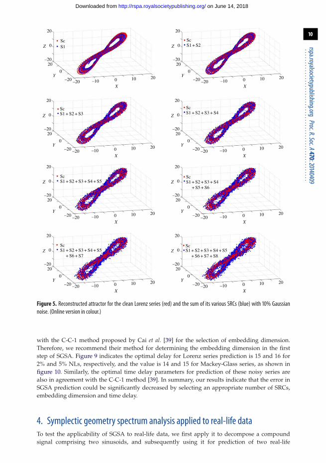
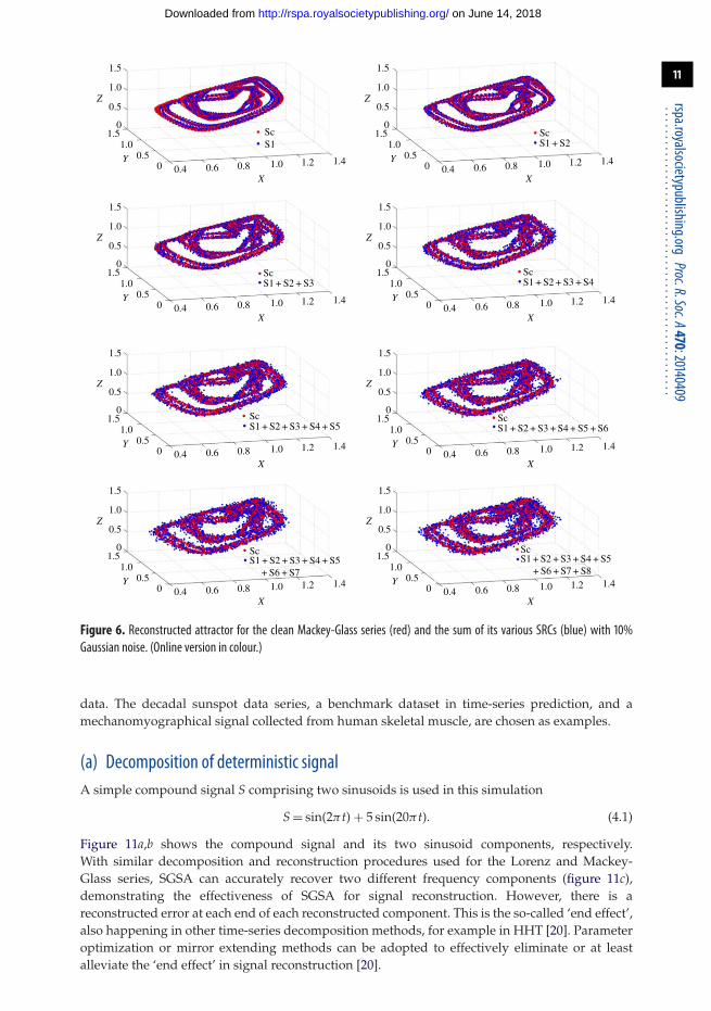
Figure 4 illustrates the symplectic geometry spectrum of the same Lorenz and Mackey-Glassseries but with various NLs ranging from 2 to 10% in steps of 2%. Although the NLs are different,the first two SRCs of both dynamic systems are almost the same for each series. We can, therefore,deduce that the first and the second SRCs contain the most information on this system. Figures 5and 6, respectively, show the reconstructed attractors of the clean Lorenz and Mackey-Glass series(red), along with that constructed from the sum of various SRCs under 10% NL (blue), in whichthe first sub-panel shows the attractor of the first SRC, until the eighth sub-panel which showsthe attractor of the sum of all SRCs. From visual inspection, the clean attractor’s envelope (red)exceeds that of the first SRC (blue) in the first sub-panel of both figures, indicating an informationloss for using only the first SRC to reconstruct the noisy attractor. However, we also observe that

on June 14, 2018http://rspa.royalsocietypublishing.org/Downloaded from

8

rspa.royalsocietypublishing.orgProc.R.Soc.A470:20140409

...................................................

–0.05

0

0.05

–0.02

0

0.02

–0.02

0

0.02

–0.02

0

0.02

–0.02

0

0.02

–0.02

0

0.02

0 500 1000 1500 2000 2500 3000–0.02

0

0.02

0

1

2

0

1

2

S1

S2

S3

S4

S5

S6

S7

S8

S

(a)

(b)

data points

Figure 3. (a) Noisy Mackey-Glass series with 10% NL. (b) Eight reconstructed components by SGSA. (Online version in colour.)

the blue envelopes of sub-panels 3–8, corresponding to the sum of the first three to eight SRCs,exceed that of the clean data (red). This implies that redundant SRCs do not contribute to theaccuracy of reconstructed attractors due to the noise component they represent. However, theclean data attractors for both series are best matched to the sum of the first two SRCs shown insub-panel 2 for each figure. This is consistent with the fact that the first and the second SRCscontain the most essential information of both systems indicated in figure 4. Therefore, it can beconcluded that the dynamic trajectory of a noisy dynamic system could be recovered by selectingan appropriate number of SRCs obtained from SGSA.

(b) Prediction of noisy chaotic time seriesA popular method for chaotic time-series prediction is the local approximation (LA) in phasespace, proposed by Farmer & Sidorowich [37]. A time series with a single dynamical variableis first embedded into a d-dimensional state space similar to that of SGSA. The dynamicalsystem generating the time series can be interpreted in the form of a nonlinear function Fτ ,

on June 14, 2018http://rspa.royalsocietypublishing.org/Downloaded from

9

rspa.royalsocietypublishing.orgProc.R.Soc.A470:20140409

...................................................

2 4 6 8

–8

–6

–4

–2

0

log(

s i/tr(

s i))

2 4 6 8the ith eigenvaluethe ith eigenvalue

2%

4%

6%8%

10%

(a) (b)

Figure 4. Symplectic geometry spectra of noisy (a) Lorenz and (b) Mackey-Glass series with NLs from 2 to 10% in steps of 2%.(Online version in colour.)

i.e. Xi+τ = Fτ Xi, where Xi and Xi+τ are the current state space and the future state space,respectively. In order to predict Xi+τ from the current state Xi, a function F̂τ that maps ad-dimensional state space to a single scalar variable of the system is employed as

xi+τ = F̂τ Xi. (3.5)

In practice, a least-square criterion is often used to determine the local F̂ for the first-orderapproximation. The value of predicted xi+τ is obtained from equation (3.5). In order to makethe prediction more than one step ahead, earlier predictions are used in constructing a newLA function F̂ [37]. In the development of the LA approach, it is assumed that the predictionaccuracy is determined by the approximation quality, which, in turn, depends on the volumeof the available data. The method is, therefore, effective for a time series consisting of aninfinite sequence of noise-free observations [38]. However, in real life, experimental observationsare inevitably corrupted by various sources of noise. In such cases, the probability that falseneighbours appear and true neighbours are rejected increases. The prediction accuracy isnaturally limited by the erroneous choice of phase space neighbours, even when increasing thenumber of observations. Moreover, the predicted values are typically iterated to obtain furtherfuture values in multi-step ahead prediction. Hence, any prediction error at a given time willpropagate and accumulate in later predictions. To improve the prediction quality, it thereforeseems useful to combine SGSA and LA into a unified method. Here, we use SGSA to filterthe initial time series before making a local prediction. For the above SRCs obtained fromnoisy Lorenz and Mackey-Glass series, we use only the sum of the first two SRCs as input toconstruct the local prediction model. Two thousand points are used for training the model andthe remaining 1000 points are used for testing. The prediction quality is evaluated in terms of thenormalized mean squared error (NMSE).

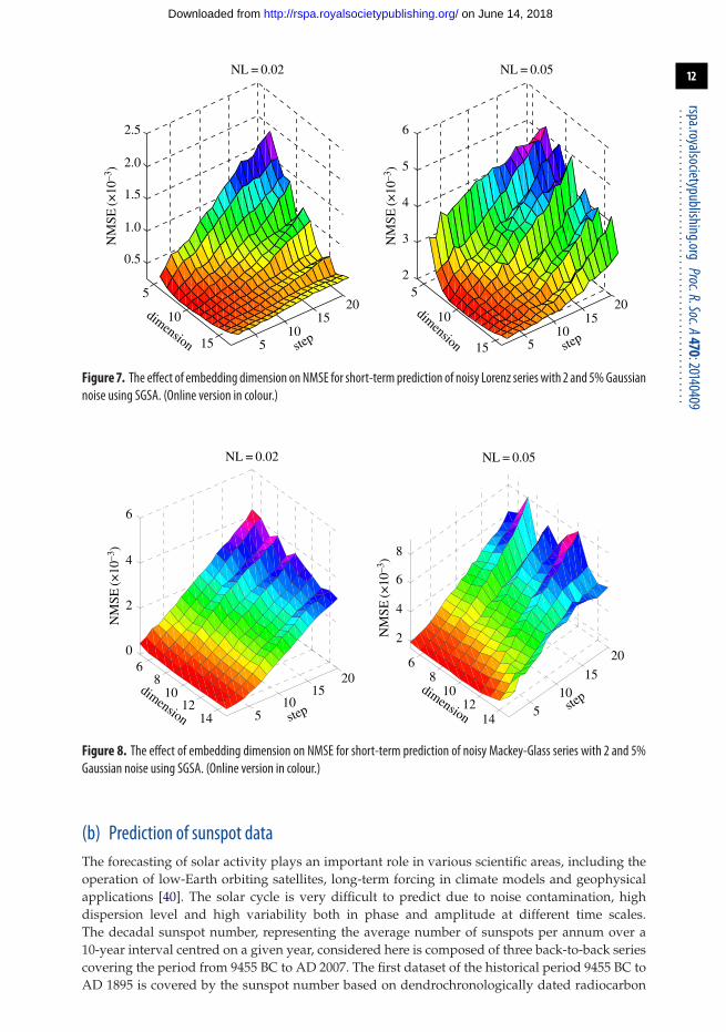
We first evaluate the NMSEs for the SGSA method on the Lorenz and Mackey-Glass series fromone- to 20-step predictions when the NL is 2 and 5%. Figures 7 and 8 show the effect of embeddingdimension on NMSE while predicting the Lorenz and Mackey-Glass series, respectively, whilefigures 9 and 10 show the effect of time delay. The prediction lead time spans from 1 to 20. Theresults shown in these figures demonstrate that appropriate SGSA embedding parameters resultin low NMSEs in prediction. For the Lorenz series, the optimal embedding dimensions are 14 and15 for 2% and 5% NLs, respectively. For the Mackey-Glass series, it is 12 and 13 for the same twoNLs, respectively. These values of optimal embedding dimensions for noisy series are consistent

on June 14, 2018http://rspa.royalsocietypublishing.org/Downloaded from

10

rspa.royalsocietypublishing.orgProc.R.Soc.A470:20140409

...................................................

20

20–20

–20 –20 –10

ScS1

0 10 20

0

0Y

X

Z

20

20–20

–20 –20 –10

ScS1 + S2

0 10 20

0

0Y

X

Z

20

20–20

–20 –20 –10

ScS1 + S2 + S3

0 10 20

0

0Y

X

Z

20

20–20

–20 –20 –10

ScS1 + S2 + S3 + S4

0 10 20

0

0Y

X

Z

20

20–20

–20 –20 –10

ScS1 + S2 + S3 + S4 + S5

0 10 20

0

0Y

X

Z

20

20–20

–20 –20 –10

ScS1 + S2 + S3 + S4 + S5 + S6

0 10 20

0

0Y

X

Z

20

20–20

–20 –20 –10

ScS1 + S2 + S3 + S4 + S5

+ S6 + S7S1 + S2 + S3 + S4 + S5

+ S6 + S7 + S8

0 10 20

0

0Y

X

Z

20

20–20

–20 –20 –10

Sc

0 10 20

0

0Y

X

Z

Figure 5. Reconstructed attractor for the clean Lorenz series (red) and the sum of its various SRCs (blue) with 10% Gaussiannoise. (Online version in colour.)

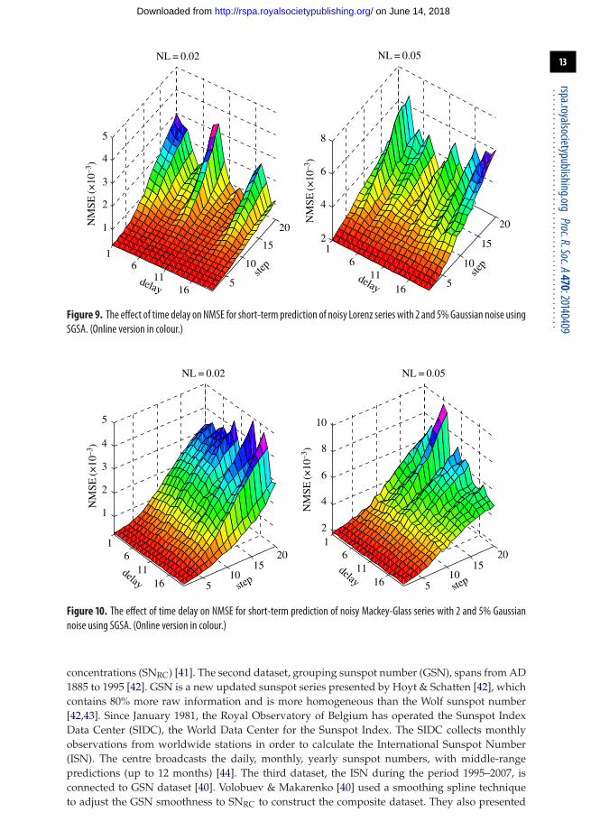
with the C-C-1 method proposed by Cai et al. [39] for the selection of embedding dimension.Therefore, we recommend their method for determining the embedding dimension in the firststep of SGSA. Figure 9 indicates the optimal delay for Lorenz series prediction is 15 and 16 for2% and 5% NLs, respectively, and the value is 14 and 15 for Mackey-Glass series, as shown infigure 10. Similarly, the optimal time delay parameters for prediction of these noisy series arealso in agreement with the C-C-1 method [39]. In summary, our results indicate that the error inSGSA prediction could be significantly decreased by selecting an appropriate number of SRCs,embedding dimension and time delay.

4. Symplectic geometry spectrum analysis applied to real-life dataTo test the applicability of SGSA to real-life data, we first apply it to decompose a compoundsignal comprising two sinusoids, and subsequently using it for prediction of two real-life

on June 14, 2018http://rspa.royalsocietypublishing.org/Downloaded from

11

rspa.royalsocietypublishing.orgProc.R.Soc.A470:20140409

...................................................

1.5

ScS1

1.5

0.5

0.50.4

X

Y

Z

0.6 0.8 1.0 1.2 1.4

0

1.0

1.0

0

1.5

ScS1 + S2

1.5

0.5

0.50.4

X

Y

Z

0.6 0.8 1.0 1.2 1.4

0

1.0

1.0

0

1.5

ScS1 + S2 + S3

1.5

0.5

0.50.4

X

Y

Z

0.6 0.8 1.0 1.2 1.4

0

1.0

1.0

0

1.5

ScS1 + S2 + S3 + S4

1.5

0.5

0.50.4

X

Y

Z

0.6 0.8 1.0 1.2 1.4

0

1.0

1.0

0

1.5

ScS1 + S2 + S3 + S4 + S5

1.5

0.5

0.50.4

X

Y

Z

0.6 0.8 1.0 1.2 1.4

0

1.0

1.0

0

1.5

ScS1 + S2 + S3 + S4 + S5 + S6

1.5

0.5

0.50.4

X

Y

Z

0.6 0.8 1.0 1.2 1.4

0

1.0

1.0

0

1.5

ScS1 + S2 + S3 + S4 + S5

+ S6 + S7

ScS1 + S2 + S3 + S4 + S5

+ S6 + S7 + S8

1.5

0.5

0.50.4

X

Y

Z

0.6 0.8 1.0 1.2 1.4

0

1.0

1.0

0

1.5

1.5

0.5

0.50.4

X

Y

Z

0.6 0.8 1.0 1.2 1.4

0

1.0

1.0

0

Figure 6. Reconstructed attractor for the clean Mackey-Glass series (red) and the sum of its various SRCs (blue) with 10%Gaussian noise. (Online version in colour.)

data. The decadal sunspot data series, a benchmark dataset in time-series prediction, and amechanomyographical signal collected from human skeletal muscle, are chosen as examples.

(a) Decomposition of deterministic signalA simple compound signal S comprising two sinusoids is used in this simulation

S = sin(2π t) + 5 sin(20π t). (4.1)

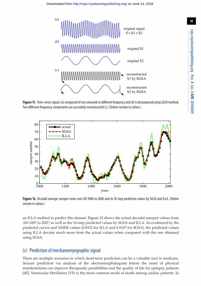
Figure 11a,b shows the compound signal and its two sinusoid components, respectively.With similar decomposition and reconstruction procedures used for the Lorenz and Mackey-Glass series, SGSA can accurately recover two different frequency components (figure 11c),demonstrating the effectiveness of SGSA for signal reconstruction. However, there is areconstructed error at each end of each reconstructed component. This is the so-called ‘end effect’,also happening in other time-series decomposition methods, for example in HHT [20]. Parameteroptimization or mirror extending methods can be adopted to effectively eliminate or at leastalleviate the ‘end effect’ in signal reconstruction [20].

on June 14, 2018http://rspa.royalsocietypublishing.org/Downloaded from

12

rspa.royalsocietypublishing.orgProc.R.Soc.A470:20140409

...................................................

510

1520

15

10

5

0.5

1.0

1.5

2.0

2.5

step

NL = 0.02

dimension

NM

SE(×

10–3

)

510

1520

15

10

52

3

4

5

6

step

NL = 0.05

dimension

NM

SE(×

10–3

)Figure 7. The effect of embedding dimension on NMSE for short-term prediction of noisy Lorenz series with 2 and 5%Gaussiannoise using SGSA. (Online version in colour.)

510

1520

1412

108

60

2

4

6

step

NL = 0.02

dimension

NM

SE(×

10–3

)

510

15

20

1412

108

6

2

4

6

8

step

NL = 0.05

dimension

NM

SE(×

10–3

)

Figure 8. The effect of embedding dimension on NMSE for short-term prediction of noisy Mackey-Glass series with 2 and 5%Gaussian noise using SGSA. (Online version in colour.)

(b) Prediction of sunspot dataThe forecasting of solar activity plays an important role in various scientific areas, including theoperation of low-Earth orbiting satellites, long-term forcing in climate models and geophysicalapplications [40]. The solar cycle is very difficult to predict due to noise contamination, highdispersion level and high variability both in phase and amplitude at different time scales.The decadal sunspot number, representing the average number of sunspots per annum over a10-year interval centred on a given year, considered here is composed of three back-to-back seriescovering the period from 9455 BC to AD 2007. The first dataset of the historical period 9455 BC toAD 1895 is covered by the sunspot number based on dendrochronologically dated radiocarbon

on June 14, 2018http://rspa.royalsocietypublishing.org/Downloaded from

13

rspa.royalsocietypublishing.orgProc.R.Soc.A470:20140409

...................................................

5

10

15

20

1611

61

1

2

3

4

5

step

NL = 0.02

delay

NM

SE(×

10–3

)

5

10

15

20

1611

61

2

4

6

8

step

NL = 0.05

delay

NM

SE(×

10–3

)Figure 9. The effect of time delay on NMSE for short-term prediction of noisy Lorenz series with 2 and 5%Gaussian noise usingSGSA. (Online version in colour.)

510

1520

1611

61

1

2

3

4

5

step

NL = 0.02

delay

NM

SE(×

10–3

)

510

1520

1611

612

4

6

8

10

step

NL = 0.05

delay

NM

SE(×

10–3

)

Figure 10. The effect of time delay on NMSE for short-term prediction of noisy Mackey-Glass series with 2 and 5% Gaussiannoise using SGSA. (Online version in colour.)

concentrations (SNRC) [41]. The second dataset, grouping sunspot number (GSN), spans from AD1885 to 1995 [42]. GSN is a new updated sunspot series presented by Hoyt & Schatten [42], whichcontains 80% more raw information and is more homogeneous than the Wolf sunspot number[42,43]. Since January 1981, the Royal Observatory of Belgium has operated the Sunspot IndexData Center (SIDC), the World Data Center for the Sunspot Index. The SIDC collects monthlyobservations from worldwide stations in order to calculate the International Sunspot Number(ISN). The centre broadcasts the daily, monthly, yearly sunspot numbers, with middle-rangepredictions (up to 12 months) [44]. The third dataset, the ISN during the period 1995–2007, isconnected to GSN dataset [40]. Volobuev & Makarenko [40] used a smoothing spline techniqueto adjust the GSN smoothness to SNRC to construct the composite dataset. They also presented

on June 14, 2018http://rspa.royalsocietypublishing.org/Downloaded from

14

rspa.royalsocietypublishing.orgProc.R.Soc.A470:20140409

...................................................

original signalS = S1 + S2

reconstructedS1 by SGSA

reconstructedS2 by SGSA

original S1

(a)

(b)

(c)

original S2

Figure 11. Time-series signal: (a) composed of two sinusoids in different frequency and (b) is decomposed using SGSAmethod.Two different frequency components are accurately reconstructed (c). (Online version in colour.)

1000 1200 1400 1600 1800 20000

10

20

30

40

50

60

70

80

suns

pot n

umbe

r

years

actualSGSAILLA

Figure 12. Decadal average sunspot series over AD 1000 to 2000 and its 10-step prediction values by SGSA and ILLA. (Onlineversion in colour.)

an ILLA method to predict this dataset. Figure 12 shows the actual decadal sunspot values fromAD 1007 to 2007, as well as the 10-step predicted values by SGSA and ILLA. As evidenced by thepredicted curves and NMSE values (0.0332 for ILLA and 0.0107 for SGSA), the predicted valuesusing ILLA deviate much more from the actual values when compared with the one obtainedusing SGSA.

(c) Prediction of mechanomyographic signalThere are multiple scenarios in which short-term prediction can be a valuable tool in medicine.Seizure prediction via analysis of the electroencephalogram before the onset of physicalmanifestations can improve therapeutic possibilities and the quality of life for epilepsy patients[45]. Ventricular fibrillation (VF) is the most common mode of death among cardiac patients. In

on June 14, 2018http://rspa.royalsocietypublishing.org/Downloaded from

15

rspa.royalsocietypublishing.orgProc.R.Soc.A470:20140409

...................................................

0 50 100 150 200 250 300 350 400 450 500–3

–2

–1

0

1

2

3

data point

MM

G a

mpl

itude

actualSGSAILLA

Figure 13. A 500-point MMG segment and its 32-step prediction by SGSA and ILLA. The MMG data are at a sample rate of1000 Hz. (Online version in colour.)

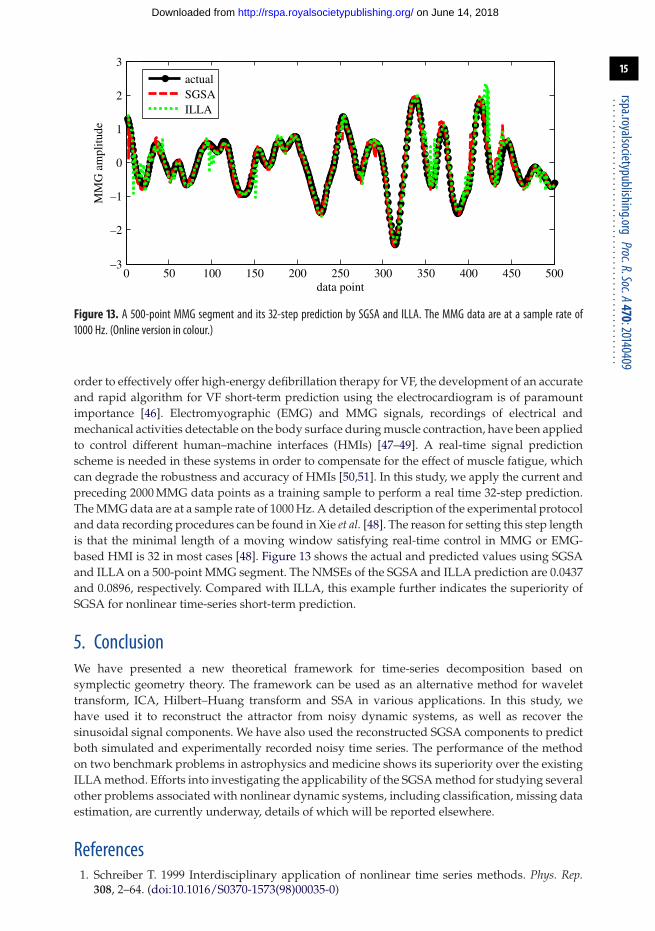
order to effectively offer high-energy defibrillation therapy for VF, the development of an accurateand rapid algorithm for VF short-term prediction using the electrocardiogram is of paramountimportance [46]. Electromyographic (EMG) and MMG signals, recordings of electrical andmechanical activities detectable on the body surface during muscle contraction, have been appliedto control different human–machine interfaces (HMIs) [47–49]. A real-time signal predictionscheme is needed in these systems in order to compensate for the effect of muscle fatigue, whichcan degrade the robustness and accuracy of HMIs [50,51]. In this study, we apply the current andpreceding 2000 MMG data points as a training sample to perform a real time 32-step prediction.The MMG data are at a sample rate of 1000 Hz. A detailed description of the experimental protocoland data recording procedures can be found in Xie et al. [48]. The reason for setting this step lengthis that the minimal length of a moving window satisfying real-time control in MMG or EMG-based HMI is 32 in most cases [48]. Figure 13 shows the actual and predicted values using SGSAand ILLA on a 500-point MMG segment. The NMSEs of the SGSA and ILLA prediction are 0.0437and 0.0896, respectively. Compared with ILLA, this example further indicates the superiority ofSGSA for nonlinear time-series short-term prediction.

5. ConclusionWe have presented a new theoretical framework for time-series decomposition based onsymplectic geometry theory. The framework can be used as an alternative method for wavelettransform, ICA, Hilbert–Huang transform and SSA in various applications. In this study, wehave used it to reconstruct the attractor from noisy dynamic systems, as well as recover thesinusoidal signal components. We have also used the reconstructed SGSA components to predictboth simulated and experimentally recorded noisy time series. The performance of the methodon two benchmark problems in astrophysics and medicine shows its superiority over the existingILLA method. Efforts into investigating the applicability of the SGSA method for studying severalother problems associated with nonlinear dynamic systems, including classification, missing dataestimation, are currently underway, details of which will be reported elsewhere.

References1. Schreiber T. 1999 Interdisciplinary application of nonlinear time series methods. Phys. Rep.

308, 2–64. (doi:10.1016/S0370-1573(98)00035-0)

on June 14, 2018http://rspa.royalsocietypublishing.org/Downloaded from

16

rspa.royalsocietypublishing.orgProc.R.Soc.A470:20140409

...................................................

2. Kantz H, Schreiber T. 2004 Nonlinear time series analysis, 2nd edn. Cambridge, UK: CambridgeUniversity Press.

3. Golyandina N, Zhigljavsky A. 2013 Singular spectrum analysis for time series. London, UK:Springer.

4. Xie HB, Wang ZZ. 2006 Mean frequency derived via Hilbert–Huang transform withapplication to fatigue EMG signal analysis. Comput. Methods Prog. Biomed. 82, 114–120. (doi:10.1016/j.cmpb.2006.02.009)

5. Chandre C, Wiggins S, Uzer T. 2003 Time-frequency analysis of chaotic systems. Phys. D 181,171–196. (doi:10.1016/S0167-2789(03)00117-9)

6. Ozkurt N, Savaci FA. 2006 Reconstruction of nonstationary signals along the wavelet ridges.Int. J. Bifurcation Chaos 16, 191–198. (doi:10.1142/S021812740601471x)

7. Han M, Liu YH, Xi JH, Guo W. 2007 Noise smoothing for nonlinear time series using waveletsoft threshold. IEEE Signal Process. Lett. 14, 62–65. (doi:10.1109/Lsp.2006.881518)

8. Ozkurt N, Savaci FA. 2005 Determination of wavelet ridges of nonstationary signalsby singular value decomposition. IEEE Trans. Circuits II. 52, 480–485. (doi:10.1109/Tcsii.2005.849041)

9. Peng ZK, Jackson MR, Rongong JA, Chu FL, Parkin RM. 2009 On the energy leakageof discrete wavelet transform. Mech. Syst. Signal. Process. 23, 330–343. (doi:10.1016/j.ymssp.2008.05.014)

10. Hyvarinen A. 1999 Fast and robust fixed-point algorithms for independent componentanalysis. IEEE Trans. Neural Netw. 10, 626–634. (doi:10.1109/72.761722)

11. Shang LJ, Shyu KK. 2009 A method for extracting chaotic signal from noisy environment.Chaos Solitons Fractals 42, 1120–1125. (doi:10.1016/j.chaos.2009.03.010)

12. Chen KY, Tung PC, Lin SL, Tsai MT. 2011 Chaos synchronization in the presence of noise. Int.J. Mod. Phys. C 22, 1409–1418. (doi:10.1142/S0129183111017007)

13. Asano H, Nakao H. 2005 Independent component analysis of spatiotemporal chaos. J. Phys.Soc. Jpn 74, 1661–1665. (doi:10.1143/Jpsj.74.1661)

14. Everson R, Roberts S. 2000 Blind source separation for non-stationary mixing. J. VLSI SignalProcess. S. 26, 15–23. (doi:10.1023/A:1008183014430)

15. Huang NE, Shen Z, Long SR, Wu MC, Shih HH, Zheng Q, Yen N-C, Tung CC, Liu HH.1998 The empirical mode decomposition and the Hilbert spectrum for nonlinear and non-stationary time series analysis. Proc. R. Soc. Lond. A 454, 903–995. (doi:10.1098/rspa.1998.0193)

16. Chavez M, Adam C, Navarro V, Boccaletti S, Martinerie J. 2005 On the intrinsic timescales involved in synchronization: a data-driven approach. Chaos 15, 023904. (doi:10.1063/1.1938467)

17. Goska A, Krawiecki A. 2006 Analysis of phase synchronization of coupled chaoticoscillators with empirical mode decomposition. Phys. Rev. E 74, 046217. (doi:10.1103/Physreve.74.046217)

18. Manchanda K, Ramaswamy R. 2011 Order parameter for the transition from strong to weakgeneralized synchrony from empirical mode decomposition analysis. Phys. Rev. E 83, 066201.(doi:10.1103/Physreve.83.066201)

19. Lee T, Ouarda TBMJ. 2011 Prediction of climate nonstationary oscillation processeswith empirical mode decomposition. J. Geophys. Res. Atmos. 116, D06107. (doi:10.1029/2010jd015142)

20. Rato RT, Ortigueira MD, Batista AG. 2008 On the HHT its problems, and some solutions.Mech. Syst. Signal. Process. 22, 1374–1394. (doi:10.1016/j.ymssp.2007.11.028)

21. Vautard R, Yiou P, Ghil M. 1992 Singular-spectrum analysis: a toolkit for short, noisy chaoticsignals. Phys. D 58, 95–126. (doi:10.1016/0167-2789(92)90103-T)

22. Istomin IA, Kotlyarov OL, Loskutov AY. 2005 The problem of processing time series:extending possibilities of the local approximation method using singular spectrum analysis.Theor. Math. Phys. 142, 128–137. (doi:10.1007/s11232-005-0077-y)

23. Wu CL, Chau KW. 2011 Rainfall-runoff modeling using artificial neural network coupled withsingular spectrum analysis. J. Hydrol. 399, 394–409. (doi:10.1016/j.jhydrol.2011.01.017)

24. Palus M, Dvorak I. 1992 Singular-value decomposition in attractor reconstruction: pitfalls andprecautions. Phys. D 55, 221–234. (doi:10.1016/0167-2789(92)90198-V)

25. Bhattacharya J, Kanjilal PP. 1999 On the detection of determinism in a time series. Phys. D 132,100–110. (doi:10.1016/S0167-2789(99)00033-0)

26. Xie HB, Wang ZZ, Huang H. 2005 Identification determinism in time series based onsymplectic geometry spectra. Phys. Lett. A 342, 156–161. (doi:10.1016/j.physleta.2005.05.035)

on June 14, 2018http://rspa.royalsocietypublishing.org/Downloaded from

17

rspa.royalsocietypublishing.orgProc.R.Soc.A470:20140409

...................................................

27. Xie HB, Dokos S. 2013 A hybrid symplectic principal component analysis and centraltendency measure method for detection of determinism in noisy time series with applicationto mechanomyography. Chaos 23, 023131. (doi:10.1063/1.4812287)

28. Xie HB, Dokos S. 2013 A symplectic geometry-based method for nonlinear time seriesdecomposition and prediction. Appl. Phys. Lett. 103, 054103. (doi:10.1063/1.4817181)

29. Lei M, Wang ZH, Feng ZJ. 2002 A method of embedding dimension estimation based onsymplectic geometry. Phys. Lett. A 303, 179–189. (doi:10.1016/S0375-9601(02)01164-7)

30. Lei M, Meng G. 2011 Symplectic principal component analysis: a new method for time seriesanalysis. Math. Probl. Eng. 2011, 793429. (doi:10.1155/2011/793429)

31. Gracia X, Munoz-Lecanda MC, Roman-Roy N. 2004 On some aspects of the geometry ofdifferential equations in physics. Int. J. Geom. Methods Mod. Phys. 1, 265–284. (doi:10.1142/S0219887804000150)

32. Ivancevic V. 2004 Symplectic rotational geometry in human biomechanics. SIAM Rev. 46,455–474. (doi:10.1137/S003614450341313x)

33. Ramirez H, Maschke B, Sbarbaro D. 2013 Modelling and control of multi-energy systems:an irreversible port-hamiltonian approach. Eur. J. Control 19, 513–520. (doi:10.1016/j.ejcon.2013.09.009)

34. Vanloan C. 1984 A symplectic method for approximating all the eigenvalues of a hamiltonianmatrix. Linear Algebra Appl. 61, 233–251. (doi:10.1016/0024-3795(84)90034-X)

35. Wu ZG, Mesbahi M. 2012 Symplectic transformation based analytical and numerical methodsfor linear quadratic control with hard terminal constraints. SIAM J. Control Optim. 50, 652–671.(doi:10.1137/090762853)

36. Chyba M, Hairer E, Vilmart G. 2009 The role of symplectic integrators in optimal control.Optim. Control Appl. Methods 30, 367–382. (doi:10.1002/Oca.855)

37. Farmer JD, Sidorowich JJ. 1987 Predicting chaotic time-series. Phys. Rev. Lett. 59, 845–848.(doi:10.1103/PhysRevLett.59.845)

38. Lim TP, Puthusserypady S. 2007 Chaotic time series prediction and additive white Gaussiannoise. Phys. Lett. A 365, 309–314. (doi:10.1016/j.physleta.2007.01.027)

39. Cai WD, Qin YQ, Yang BR. 2008 Determination of phase-space reconstruction parameters ofchaotic time series. Kybernetika 44, 557–570.

40. Volobuev DM, Makarenko NG. 2008 Forecast of the decadal average sunspot number. SolarPhys. 249, 121–133. (doi:10.1007/s11207-008-9167-y)

41. Solanki SK, Usoskin IG, Kromer B, Schussler M, Beer J. 2004 Unusual activity of thesun during recent decades compared to the previous 11,000 years. Nature 431, 1084–1087.(doi:10.1038/Nature02995)

42. Hoyt DV, Schatten KH. 1998 Group sunspot numbers: a new solar activity reconstruction.Solar Phys. 181, 491–512. (doi:10.1023/A:1005056326158)

43. Usoskin IG, Kovaltsov GA. 2004 Long-term solar activity: direct and indirect study. Solar Phys.224, 37–47. (doi:10.1007/s11207-005-3997-7)

44. Vanlommel P, Cugnon P, Van der Linden RAM, Berghmans D, Clette F. 2004 The SIDC: worlddata center for the sunspot index. Solar Phys. 224, 113–120. (doi:10.1007/s11207-005-6504-2)

45. Mormann F, Andrzejak RG, Elger CE, Lehnertz K. 2007 Seizure prediction: the long andwinding road. Brain 130, 314–333. (doi:10.1093/Brain/Awl241)

46. Huang H, Xie HB, Wang ZZ. 2005 The analysis of vf and vt with wavelet-based tsallisinformation measure. Phys. Lett. A 336, 180–187. (doi:10.1016/j.physleta.2004.12.090)

47. Orizio C. 1993 Muscle sound: bases for the introduction of a mechanomyographic signal inmuscle studies. Crit. Rev. Biomed. Eng. 21, 201–243.

48. Xie HB, Zheng YP, Guo JY. 2009 Classification of the mechanomyogram signal using a waveletpacket transform and singular value decomposition for multifunction prosthesis control.Physiol. Meas. 30, 441–457. (doi:10.1088/0967-3334/30/5/002)

49. Alves N, Chau T. 2010 Uncovering patterns of forearm muscle activity using multi-channelmechanomyography. J. Electromyogr. Kinesiol. 20, 777–786. (doi:10.1016/j.jelekin.2009.09.003)

50. Winslow J, Jacobs PL, Tepavac D. 2003 Fatigue compensation during FES using surface EMG.J Electromyogr Kinesiol. 13, 555–568. (doi:10.1016/S1050-6411(03)00055-5)

51. Park EJ, Meek SG. 1993 Fatigue compensation of the electromyographic signal for prostheticcontrol and force estimation. IEEE Trans. Biomed. Eng. 40, 1019–1023. (doi:10.1109/10.247800)

on June 14, 2018http://rspa.royalsocietypublishing.org/Downloaded from