Embed Size (px)
Citation preview
Commun. Comput. Phys.doi: 10.4208/cicp.311012.191113a
Vol. 16, No. 1, pp. 169-200July 2014
High-Order Symplectic Schemes for Stochastic
Hamiltonian Systems
Jian Deng1,∗, Cristina Anton2 and Yau Shu Wong1
1 Department of Mathematical and Statistical Sciences, University of Alberta,Edmonton, AB T6G 2G1, Canada.2 Department of Mathematics and Statistics, Grant MacEwan University,Edmonton, AB T5J 4S2, Canada.
Received 31 October 2012; Accepted (in revised version) 19 November 2013
Available online 10 April 2014
Abstract. The construction of symplectic numerical schemes for stochastic Hamilto-nian systems is studied. An approach based on generating functions method is pro-posed to generate the stochastic symplectic integration of any desired order. In generalthe proposed symplectic schemes are fully implicit, and they become computationallyexpensive for mean square orders greater than two. However, for stochastic Hamil-tonian systems preserving Hamiltonian functions, the high-order symplectic methodshave simpler forms than the explicit Taylor expansion schemes. A theoretical analysisof the convergence and numerical simulations are reported for several symplectic inte-grators. The numerical case studies confirm that the symplectic methods are efficientcomputational tools for long-term simulations.
AMS subject classifications: 60H10, 65C30, 65P10
Key words: Stochastic Hamiltonian systems, symplectic integration, mean-square convergence,high-order schemes.
1 Introduction
The symplectic integration covers a special type of numerical methods which are capa-ble of preserving the symplecticity properties of the Hamiltonian system. The pioneeringwork on the symplectic integration is due to de Vogelaere [1], Ruth [2] and Kang Feng [3].Symplectic methods have been applied successfully to deterministic Hamiltonian sys-tems, and numerical simulations consistently show that the most important feature ofthis approach is that the accuracy of the computed solution is guaranteed even for long
∗Corresponding author. Email addresses: [email protected] (J. Deng), [email protected] (C. Anton),[email protected] (Y. S. Wong)
http://www.global-sci.com/ 169 c©2014 Global-Science Press
170 J. Deng, C. Anton and Y. S. Wong / Commun. Comput. Phys., 16 (2014), pp. 169-200
term computation [4, 5]. In this paper, we study the symplectic numerical integration forstochastic Hamiltonian systems, and propose an approach to generate symplectic numer-ical schemes of any desired order.
Consider the stochastic differential equations (SDEs) in the sense of the Stratonovich:
dPi =−∂H(0)(P,Q)
∂Qidt−
m
∑r=1
∂H(r)(P,Q)
∂Qi◦dwr
t , P(t0)= p, (1.1a)
dQi =∂H(0)(P,Q)
∂Pidt+
m
∑r=1
∂H(r)(P,Q)
∂Pi◦dwr
t , Q(t0)=q, (1.1b)
where P, Q, p, q are n-dimensional vectors with components Pi, Qi, pi, qi, i=1,··· ,n andwr
t , r=1,··· ,m are independent standard Wiener Processes. The SDEs (1.1) are called theStochastic Hamiltonian System (SHS) (see [6]). The SHS (1.1) includes both Hamiltoniansystems with additive or multiplicative noise.
A non-autonomous SHS is given by time-dependent Hamiltonian functionsH(r)(t,P,Q), r = 0,··· ,m. However, it can be rewritten as an autonomous SHS by intro-ducing new variables ek and fk. Let
d fr =dt, der =−∂H(r)(t,P,Q)
∂t◦dwr
t , (where dw0t :=dt),
with the initial condition er(t0) = −H(r)(t0,p,q) and fr(t0) = t0, r = 0,··· ,m. Then thenew Hamiltonian functions H(r)(P,Q) = H(r)( fr,P,Q), r = 1,··· ,m, and H(0)(P,Q) =H(0)( fr,P,Q)+e0+···+em, define an autonomous SHS with P=(PT,e0,··· ,em)T and Q=(QT, f0,··· , fm)T. Hence, in this study, we will only investigate the autonomous case asgiven in (1.1).
There are growing interests and efforts on the theoretical study and computationalimplementation of numerical methods for SHS [6, 8–11]. Milstein et al. [6, 8] introducedthe symplectic numerical schemes to SHS, and demonstrated the superiority of the sym-plectic methods for long time computation. Although they proposed symplectic schemesof orders two or three for special types of SHS, for the general SHS with multiplicativenoise given in (1.1), they construct only symplectic schemes of mean square order 0.5.In this paper we apply an approach based on generating functions and we constructsymplectic schemes of arbitrary high mean square order. Hong et al. [9] developed apredictor-corrector scheme for a linear SDE with an additive noise, a simple case of SHS.In [11], Wang et al. proposed the variational integrators to construct the stochastic sym-plectic schemes.
The generating functions associated with the SHS (1.1) were rigorously introducedin [15]. Recently, Wang et al. [12–14] proposed generating functions methods to con-struct symplectic schemes for SHS. But, in those papers, only the product of one-foldStratonovich integrals is considered, so their approach cannot be used to construct
J. Deng, C. Anton and Y. S. Wong / Commun. Comput. Phys., 16 (2014), pp. 169-200 171
stochastic symplectic scheme higher than order 1.5. In this paper, the product of mul-tiple Stratonovich integrals (Property 3.1) is studied, such that the generating functionscan be used to construct symplectic schemes of arbitrary order.
We follow the rigorous approach presented in [15], and employ the properties of mul-tiple stochastic integrals to derive a recursive formula for determining the coefficientsof the generating function. Theoretically, this formula allow us to construct stochasticsymplectic schemes of arbitrary high order with corresponding conditions on the Hamil-tonian functions. Hence, the major contribution of the work reported here is to presenta way for finding the coefficients of the generating functions such that the generatingfunction method could be used to construct stochastic symplectic schemes of any order.Since the computation complexity increases with the order of the numerical schemes, wemainly focus on the symplectic schemes with mean square order 1 for which we alsopresent the convergence analysis. Moreover, for special types of SHSs, such as SHSs withadditive noise, SHSs with separable Hamiltonians, or SHS preserving the Hamiltonianfunctions, we construct computationally attractive symplectic schemes of mean squareorder 2. The study of high order stochastic symplectic scheme for the general SHS (1.1)helps to construct high order Runge-Kutta type schemes that avoid higher order deriva-tives.
The paper is organized as follow. In the beginning, we present the theory of gen-erating functions and Hamiltonian-Jacobi partial differential equations in the stochasticsetting. The construction of the symplectic schemes based on approximating of the so-lution of the corresponding Hamilton-Jacobi stochastic partial differential equations ispresented in Section 3. In Section 4, we construct higher order symplectic schemes, andin Section 5 we study the convergence of these schemes. Symplectic schemes for specialtypes of SHSs are included in Section 6. Numerical simulations illustrating the perfor-mance of the proposed methods are reported in Section 7.
2 Generating function and Stochastic Hamilton-Jacobi partial
differential equation
The generating function applied to the deterministic Hamiltonian system has been wellstudied. However, the extension to stochastic cases is a challenging task.
We denote the solution of the SHS (1.1) by
X(t;t0,x0;ω)=(
PT(t;t0,p,q;ω),QT(t;t0,p,q;ω))T
,
where t0≤ t≤ t0+T, and ω is an elementary event. It is known that if H(j), j=0,··· ,m, aresufficiently smooth, then X(t;t0,x0;ω) is a phase flow (diffeomorphism) for almost anyω (see [7]). To simplify the notation, we will remove any mentioning of the dependenceon ω unless it is absolutely necessary to avoid confusions, and we make the conventionto understand that all the equations involving the solution of the SHS (1.1) are true foralmost any ω.
172 J. Deng, C. Anton and Y. S. Wong / Commun. Comput. Phys., 16 (2014), pp. 169-200
In differential geometry, the differential 1-form of a function f :R2n →R on ξ∈R2n isdefined as:
d f (ξ) :=2n
∑i=1
∂ f
∂ziξi. (2.1)
The exterior product d f ∧dg of ξ,η ∈ R2n is given by d f ∧dg(ξ,η) = d f (ξ)dg(η)−d f (η)dg(ξ), and represents the oriented area of the image of the parallelogram with sidesd f (ξ) and dg(η) on the d f (ξ), dg(η)-plane.
The stochastic flow (p,q)→ (P,Q) of the SHS (1.1) preserves the symplectic structure(Theorem 2.1 in [6]) as follows:
dP∧dQ=dp∧dq, (2.2)
i.e., the sum over the oriented areas of its projections onto the two dimensional plane(pi,qi) is invariant. Here we consider the differential 2-form
dp∧dq=dp1∧dq1+···+dpn∧dqn, (2.3)
and the differentiation in (1.1) and (2.2) have different meanings: in (1.1) p, q are fixedparameters and differentiation is done with respect to time t, while in (2.2) differentiationis carried out with respect to the initial data p, q. We say that a method based on the onestep approximation P=P(t+h;t,p,q), Q=Q(t+h;t,p,q) preserves the symplectic structureif
dP∧dQ=dp∧dq. (2.4)
The previous definition of symplecticity can be extended to general random maps. Arandom map ϕ(ω,x) is a map with the property that for any fixed x ∈R2n, ϕ(·,x) is arandom variable. We denote ϕω(·)= ϕ(ω,·). According to (2.2) a random differentiablemap ϕω : (p,q)→ (P,Q) is symplectic if and only if dP∧dQ = dp∧dq a.s. We can easilyprove the following equivalent property.
Proposition 2.1. A differentiable random map ϕω : U →R2n (where U ⊂R2n is an open
set) is symplectic if and only if the Jacobian matrix ϕ′ω satisfies
ϕ′(p,q)T Jϕ′(p,q)= J with J=
[
0 I−I 0
]
, (2.5)
for almost any ω and any p,q∈Rn , (p,q)T∈U, where I is the identity matrix of dimensionn.
In the deterministic case, generating functions are powerful tools to study symplectictransformations. The next lemma introduces the generating functions Sω, Si
ω, i=1,2,3 inthe stochastic case.
Lemma 2.1. Let ϕω : (p,q)→ (P,Q) be a smooth random map from R2n to R2n. Then ϕω is
symplectic if any of the following statements is true:
J. Deng, C. Anton and Y. S. Wong / Commun. Comput. Phys., 16 (2014), pp. 169-200 173
1. There exists locally a smooth random map Sω from R2n to R2n such that ∂(Sω)/∂q∂Q is
invertible a.s. and we have
Pi=∂S
∂Qi(q,Q), pi =− ∂S
∂qi(q,Q), i=1,··· ,n. (2.6)
2. There exists locally a smooth random map S1ω fromR2n toR2n such that ∂(PTq+S1
ω)/∂P∂qis invertible a.s. and we have
pi =Pi+∂S1
ω
∂qi(P,q), Qi =qi+
∂S1ω
∂Pi(P,q), i=1,··· ,n. (2.7)
3. There exists locally a smooth random map S2ω from R
2n to R2n such that ∂(pTQ+S2
ω)/∂p∂Q is invertible a.s. and we have
qi =Qi+∂S2
ω
∂pi(p,Q), Pi= pi+
∂S2ω
∂Qi(p,Q), i=1,··· ,n. (2.8)
4. There exists locally a smooth random map S3ω from R
2n to R2n such that ∂((P+p)T(Q−q)−2S3
ω)/∂Y∂y is invertible a.s. and we have
Y=y− J∇S3ω((y+Y)/2), (2.9)
where Y=(PT,QT)T, y=(pT ,qT)T.
Proof. The proof can be completed easily by adapting the proof of Theorem 3.1 in [8].
The previous lemma gives us a powerful tool to analyze the symplectic structure andto construct symplectic methods. For instance, for the SHS (1.1), if in the relation (2.7) welet
S1ω =hH(0)(P,q)+
h
2
m
∑r=1
n
∑j=1
∂H(r)
∂qj(P,q)
∂H(r)
∂Pj(P,q)+
m
∑r=1
√hξr H(r)(P,q), (2.10)
where h is the time step and ξr are independent bounded random variables such thatE(ξr−ξ)2 ≤ h, with ξ ∼ N(0,1), then we obtain the symplectic Euler scheme proposedby Milstein et al. [6, 8]. Lemma 2.1 guarantees that the numerical scheme is symplectic.Moreover the implicit midpoint scheme in [8] is obtained by setting
S3ω =hH(0)((y+Y)/2)+
m
∑r=1
√hξr H(r)((y+Y)/2) (2.11)
in relation (2.9).We introduce the stochastic Hamilton-Jacobi partial differential equation (HJ PDE)
associated with the SHS (1.1) following the rigorous approach from [15]. We want toconsider the effect of time in the generating function Sω, so let Sω(x,t) be a family of real
174 J. Deng, C. Anton and Y. S. Wong / Commun. Comput. Phys., 16 (2014), pp. 169-200
valued processes with parameters x∈R2n. We can regard it as random field with doubleparameters x and t. If Sω(x,t) is a C∞ function of x for almost all ω for any t, we canregard Sω(x,t) as a C∞ value process [7].
Let assume that the Hamiltonian function H(r) for r=0,··· ,m in (1.1) belong to C∞. Inaddition, we also suppose that:
m
∑r=0
(|∇pH(r)(P,Q)−∇pH(r)(p,q)|+|∇q H(r)(P,Q)−∇qH(r)(p,q)|)
≤L1(|P−p|+|Q−q|) (2.12)
andm
∑r=0
(|∇pH(r)(p,q)|+|∇q H(r)(p,q)|)≤ L2(1+|p|+|q|). (2.13)
So the Lipschitz condition (2.12) and linear growth bound (2.13) guarantees the localexistence and uniqueness of the solution (P(t,ω)T,Q(t,ω)T)T of the SHS (1.1). Moreover,
it is known that X(t;t0,x0;ω)=(
PT(t;t0,p,q;ω), QT(t;t0,p,q;ω))T
, where t0 ≤ t≤ t0+T isa diffeomorphism a.s. [7]. Thus the generating function, which is a random mapping,becomes a stochastic process S(q,Q,t,ω), and through Eq. (2.6), this stochastic processgenerates the symplectic map (p,q)→ (P(t,ω),Q(t,ω)) of the flow of the SHS.
For the sake of simplification, let us keep the notation Sω for the stochastic processS(q,Q,t,ω). The generating function Sω is connected with the SHS (1.1) by the Hamilton-Jacobi partial differential equation (HJ PDE) (see Theorem 6.14 in [15]):
dSω =−H(0)( ∂Sω
∂Q1,··· , ∂Sω
∂Qn,Q1,··· ,Qn
)
dt
−m
∑r=1
H(r)( ∂Sω
∂Q1,··· , ∂Sω
∂Qn,Q1,··· ,Qn
)
◦dwrt , (2.14)
with the initial condition Sω(q,Q,0) = j(q,Q), where j is a C∞ function. Starting fromthe flow X(t;t0,x0;ω) of the SHS (1.1) and using the method of characteristics, in Theo-rem 6.14 and its corollary in [15] it is shown that for any initial point x0 there exists astopping time τ > t0 a.s and a local solution Sω(q,Q,t), t0 ≤ t< τ of (2.14) for which wehave the equations given in (2.6). Moreover, almost sure the flow X(t;t0,x0;ω) is a lo-cal Stratonovich semi-martingale, and Sω(q,Q,t), ∂Sω(q,Q,t)/∂Q and ∂Sω(q,Q,t)/∂q arelocal Stratonovich semi-martingale, continuous on (q,Q,t), and C∞ value processes (seealso Theorem 6.1.5 in [7]).
Theorem 2.1. Let Sω(q,Q,t) be a local solution of the HJ PDE (2.14) with initial values satisfy-ing
∂j
∂qi(q,q)+
∂j
∂Qi(q,q)=0, i=1,··· ,n,
J. Deng, C. Anton and Y. S. Wong / Commun. Comput. Phys., 16 (2014), pp. 169-200 175
and such that almost sure Sω(q,Q,t), ∂Sω(q,Q,t)/∂Q and ∂Sω(q,Q,t)/∂q are localStratonovich semi-martingale, continuous on (q,Q,t), and C∞ value processes. If there existsa stopping time τ′
> t0 a.s. such that the matrix (∂2(Sω)/∂q∂Q) is a.s. invertible for t0 ≤ t<τ′ ,then the map (p,q)→(P(t,ω),Q(t,ω)), t0≤ t<τ′, defined by (2.6) is the flow of the SHS (1.1).
Proof. The mapping (p,q)→ (Pω,Qω) is well defined by (2.6) because of the invertibilityof the matrix (∂2(Sω)/∂q∂Q) for t0≤ t<τ′, and the implicit function theorem.
Differentiation of the second equation of (2.6) (see Theorem 3.3.2 in [7]) yields
d( ∂Sω
∂qi
)
+n
∑j=1
∂2Sω
∂qi∂QjdQj =0. (2.15)
Recalling that Sω is the solution of the stochastic HJ PDE (2.14), the following equa-tion holds by differentiating (2.14) with respect to qi (see the Corollary of Theorem 6.14in [15]).
d(∂Sω
∂qi
)
+n
∑j=1
∂H(0)
∂Pj
∂2Sω
∂qi∂Qjdt+
m
∑r=1
n
∑j=1
∂H(r)
∂Pj
∂2Sω
∂qi∂Qj◦dwr
t =0. (2.16)
Comparing Eqs. (2.15) and (2.16) and using the invertibility of the matrix (∂2Sω/∂qi∂Qj),we have the second equation of (1.1).
The first equation of (1.1) can be obtained using a similar procedure as reportedabove, i.e., by differentiating the first relation of (2.6) and the HJ PDE with respectto Qi, then subtracting the obtained equations. Also the initial values guarantee that(P(t0,ω),Q(t0,ω))=(p,q).
The HJ PDEs for the coordinate transformations (2) and (4) in Lemma 2.1 can be ex-pressed as
S1ω(t,P,q)=
∫ t
t0
H(0)(P,q+∇PS1ω(s,P,q))ds
+∫ t
t0
m
∑r=1
H(r)(P,q+∇PS1ω(s,P,q))◦dwr
s , (2.17a)
S3ω(t,w)=
∫ t
t0
H(0)(
w+1
2J−1∇S3
ω(s,w))
ds
+∫ t
t0
m
∑r=1
H(r)(
w+1
2J−1∇S3
ω(s,w))
◦dwrs, (2.17b)
where w∈R2n, and we consider S1ω|t=t0 =0 and S3
ω|t=t0 =0. It is straightforward to obtainthe HJ PDE for the generating function (3) in Lemma 2.1, as it is just the adjoint case of(2).
176 J. Deng, C. Anton and Y. S. Wong / Commun. Comput. Phys., 16 (2014), pp. 169-200
3 Constructing high-order symplectic schemes
For deterministic problems, the construction of high-order symplectic schemes via gen-erating functions was first proposed by Kang Feng et al. [3, 17]. The key idea is to obtainan approximation of the solution of the HJ PDE, and then to construct the symplecticnumerical scheme through the relations (2.7)-(2.9).
Following this idea, we now seek an expansion which reflects the stochastic proper-ties of the generating function. Due to the Ito representation theorem, the relation be-tween the Ito integral, the Stratonovich integral and the stochastic Taylor-Stratonovichexpansion, it is reasonable to assume that the generating function can be expressed bythe following expansion locally:
S1(P,q,t,θ(t)ω)=G1(0)(P,q)J(0)+G1
(1)(P,q)J(1)+G1(0,1)(P,q)J(0,1)+···=∑
α
G1α Jα, (3.1)
where α=(j1, j2,··· , jl), ji ∈{0,1,··· ,m}, i=1,··· ,l is a multi-index of length l, and Jα is themultiple Stratonovich integral
Jα =∫ t
0
∫ sl
0···∫ s2
0◦dw
j1s1···◦dw
jl−1sl−1
◦dwjlsl
. (3.2)
For convenience, ds is denoted by dw0s . Similarly, the multiple Ito stochastic integral Iα is
given by
Iα=∫ t
0
∫ sl
0···∫ s2
0dw
j1s1···dw
jl−1sl−1
dwjlsl
. (3.3)
3.1 Properties of multiple stochastic integrals
To prepare for the derivation of the symplectic numerical schemes, we discuss someproperties of the multiple stochastic integrals. First, we define some operations for multi-indexes.
If the multi-index α = (j1, j2,··· , jl) with l > 1 then α−= (j1, j2,··· , jl−1), i.e., the lastcomponent is deleted. For instance, (1,3,0)− = (1,3). For any two multi-indexesα = (j1, j2,··· , jl) and α′ = (j′1, j′2,··· , j′l′), we define the concatenation operation ∗ asα∗α′ = (j1, j2,··· , jl , j′1, j′2,··· , j′l′). For example, (1,3,0)∗(1,4) = (1,3,0,1,4). The concate-nation of a collection Λ of multi-indexes with the multi-index α gives the collectionformed by concatenating each element of the collection Λ with the multi-index α, i.e.,Λ∗α= {α′∗α|α′ ∈Λ}. For example, if Λ= {(1,1),(0,1,2),(1,1)} and α=(0), then Λ∗α={(1,1,0),(0,1,2,0),(1,1,0)}.
Proposition 3.1. For
Jα Jα′ = ∑β∈Λα,α′
Jβ, (3.4)
J. Deng, C. Anton and Y. S. Wong / Commun. Comput. Phys., 16 (2014), pp. 169-200 177
where α = (j1, j2,··· , jl), α′ = (j′1, j′2,··· , j′l′) and Λα,α′ is the collection of multi-indexes de-pending on α and α′, and given by the following recurrence relation:
Λα,α′ =
{(j1, j′1),(j′1, j1)}, if l=1 and l′=1,
{Λ(j1),α′−∗(j′l′),α′∗(jl)}, if l=1 and l′ 6=1,
{Λα−,(j′1)∗(jl),α∗(j′l)}, if l 6=1 and l′=1,
{Λα−,α′∗(jl),Λα,α′−∗(j′l′)}, if l 6=1 and l′ 6=1.
(3.5)
Proof. Let consider two stochastic processes
X1t =
∫ t
0b1(Xs)◦dw
jls and X2
t =∫ t
0b2(Xs)◦dw
j′l′
s . (3.6)
Then, for the Stratonovich integrals, we have
X1t X2
t =∫ t
0X2
s b1(Xs)◦dwjls +
∫ t
0X1
s b2(Xs)◦dwj′l′
s . (3.7)
If l > 1 and l′> 1, let b1(Xs)= Jα− and b2(Xs)= J′α′−, such that X1t = Jα and X2
t = Jα′ . Theproduct rule (3.7) of the stochastic integrals yields
Jα Jα′ =∫ t
0Jα′ Jα−◦dw
jls +
∫ t
0Jα Jα′−◦dw
j′l′
s . (3.8)
This implies the fourth relation in (3.5).
If l = 1 (or l′= 1), the second (or third) relation in the recurrence (3.5) is obtained forb1(Xs)=1 and b2(Xs)= J′α′− (or b1(Xs)= Jα− and b2(Xs)=1). For the first relation, we takeb1(Xs)=1 and b2(Xs)=1.
For instance, since
Λ(2,0),(0,1)={Λ(2),(0,1)∗(0),Λ(2,0),(0)∗(1)}={{Λ(2),(0)∗(1),(0,1,2)}∗(0)},{Λ(2),(0)∗(0),(2,0,0)}∗(1)}={{(2,0,1),(0,2,1),(0,1,2)}∗(0),{(0,2,0),(2,0,0),(2,0,0)}∗(1)}={(2,0,1,0),(0,2,1,0),(0,1,2,0),(0,2,0,1),(2,0,0,1),(2,0,0,1)}, (3.9)
then we have J(2,0) J(0,1)= J(2,0,1,0)+ J(0,2,1,0)+ J(0,1,2,0)+ J(0,2,0,1)+2J(2,0,0,1).
Remark 3.1. From the recurrence (3.5), we can see that Λα,α′ = Λα′,α, and the length ofthe multi indexes in Λα,α′ is the summation of the lengths of α and α′, i.e., if β ∈ Λα,α′ ,then l(β)= l(α)+l(α′). This will be used to determine the coefficients of the generatingfunction in the next subsection.
178 J. Deng, C. Anton and Y. S. Wong / Commun. Comput. Phys., 16 (2014), pp. 169-200
Corollary 3.1. For α=(j1, j2,··· , jl),
wjt Jα=
l
∑i=0
J(j1 ,···,ji ,j,ji+1,···,jl). (3.10)
Proof. The proof follows by repeatedly applying the second recurrence of (3.5).
Similarly, we can show that the multiplication of a finite sequence of multiple-indexescan be expressed by the following summation:
n
∏i=1
Jαi= ∑
β∈Λα1,···,αn
Jβ, (3.11)
where the collection Λα1,···,αn can be defined recursively by Λα1,···,αn = {Λβ,αn|β ∈
Λα1,···,αn−1}, n≥ 3. For example, Λ(1),(0),(0)= {Λβ,(0)|β∈Λ(1),(0)}= {Λ(0,1),(0),Λ(1,0),(0)}=
{(0,0,1),(0,0,1),(0,1,0),(1,0,0),(0,1,0),(1,0,0)}. Thus J(1) J2(0)=2J(0,0,1)+2J(1,0,0)+2J0,1,0).
In addition to the recurrence relation (3.5), we also propose an explicit way to cal-culate the collection Λα,α′ . First, for any multi-index α=(j1, j2,··· , jl) with no duplicatedelements (i.e., jm 6= jn if m 6= n, m,n= 1,··· ,l), we define the set R(α) to be the empty setR(α)=Φ if l = 1 and R(α)= {(jm, jn)|m< n,m,n= 1,··· ,l} if l ≥ 2. R(α) defines a partialorder on the set formed with the numbers included in the multi-index α, defined by i≺ jif and only if (i, j)∈R(α). We suppose that there are no duplicated elements in or betweenthe multi-indexes α=(j1, j2,··· , jl) and α′=(j′1, j′2,··· , j′l′).Lemma 3.1. If there is no duplicated elements in or between the multi-indexes α=(j1, j2,··· , jl)and α′=(j′1, j′2,··· , j′l′), then
Λα,α′ ={β∈M|l(β)= l(α)+l(α′),R(α)∪R(α′)⊆R(β)
and β has no duplicated elements}, (3.12)
where M={( j1, j2,··· , jl+l′)| ji ∈{j1, j2,··· , jl, j′1, j′2,··· , j′l′}, i=1,··· ,l+l′}.
Proof. Let denote Λ′α,α′ = {β ∈M|l(β) = l(α)+l(α′), R(α)∪R(α′) ⊆ R(β) and β has no
duplicated elements }. Since there are no duplicated elements in β and l(β)= l(α)+l(α′),each element of {j1, j2,··· , jl, j′1, j′2,··· , j′l′} must appear in β only once.
We prove that Λα,α′ =Λ′α,α′ by induction on l(α)+l(α′). If l(α)+l(α′)=2, then l(α)=
l(α′)= 1 and R(α)=R(α′)=Φ. Hence R(β) contains any pair with distinct componentsfrom M={( j1, j2)| j1, j2∈{j1, j′1}}, so Λ′
α,α′={(j1, j′1),(j′1, j1)}, and from the first equation inthe recurrence (3.5), Λ′
α,α′ =Λα,α′ .We suppose that Λα,α′ =Λ′
α,α′ for any multi-indexes α and α′ such that l(α)+l(α′)< kand we prove that Λα,α′ =Λ′
α,α′ for any multi-indexes α and α′ with l(α)+l(α′)= k.
First, we now prove that Λ′α,α′ ⊆Λα,α′. For any element β= { j1, j2,··· , jk} in Λ′
α,α′ , be-cause jl is the largest element with respect to the partial order defined by R(α), and j′l′ is
the largest element with respect to the partial order defined by R(α′), then jk can only bejl or j′l′ . This leads to the following cases:
J. Deng, C. Anton and Y. S. Wong / Commun. Comput. Phys., 16 (2014), pp. 169-200 179
1. If jk = jl and l=1, then β=α′∗ j1 ∈Λα,α′ , by the second equation in recurrence (3.5).
2. If jk = jl and l > 1, then β−∈Λ′α−,α′ =Λα−,α′ by the induction assumption because
l(α−)+l(α′)=k−1<k. Hence β=β−∗(jl)∈Λα−,α′∗(jl), and from the fourth equationin recurrence (3.5) we get β∈Λα,α′ .
3. If jk = jl′ and l′=1, then β=α∗ j′1 ∈Λα,α′ , by the third equation in recurrence (3.5).
4. If jk = jl′ and l′>1, then β−∈Λ′α,α′−=Λα,α′−. Hence β= β−∗(j′l )∈Λα,α′−∗(j′l), and
from the fourth equation in recurrence (3.5) we get β∈Λα,α′ .
Similarly, using the recurrence (3.5), we can prove that Λα,α′⊆Λ′α,α′ . Thus Λα,α′=Λ′
α,α′
and the lemma is proved.
The lemma can be easily extended to determine the collection Λα1,···,αn .
Lemma 3.2. If there are no duplicated elements in or between any of the multi-indexes α =
(j(1)1 , j
(1)2 ,··· , j(1)l1
), ··· , αn =(j(n)1 , j
(n)2 ,··· , j(n)ln
), then
Λα1,···,αn ={
β∈M|l(β)=n
∑k=1
l(αk)and ∪nk=1 R(αk)⊆R(β)
and there are no duplicated elements in β}
, (3.13)
where M={
( j1, j2,··· , jl)| ji∈{j(1)1 , j
(1)2 ,··· , j(1)l1
,··· , j(n)1 , j(n)2 ,··· , j(n)ln
}, i=1,··· , l, l= l1+···+ln
}
.
To extend the previous two lemmas to multi-indexes with duplicated ele-ments, we just need to assign a different subscript to each duplicated element,for example, Λ(2,0),(0,1) = Λ(2,01),(02,1) = {(2,02,1,01),(02,2,1,01),(01,1,2,02),(02,2,01,1),(2,01,02,1),(2,02,01,1)}.
3.2 Higher order symplectic scheme
Inserting (3.1) into the HJ PDE (2.17a), and using the proposition (3.1), we get
S1ω =
∫ t
0H(0)
(
P,q+∑α
∂G1α
∂PJα
)
ds+m
∑r=1
∫ t
0H(r)
(
P,q+∑α
∂G1α
∂PJα
)
◦dwrs
=m
∑r=0
∫ t
0H(r)
(
P,q+∑α
∂G1α
∂PJα
)
◦dwrs
=m
∑r=0
∫ t
0
∞
∑i=0
1
i!
n
∑k1,···,ki=1
∂iH(r)
∂qk1···∂qki
(
∑α
∂G1α
∂PJα
)
k1
···(
∑α
∂G1α
∂PJα
)
ki
◦dwrs
=m
∑r=0
∞
∑i=0
1
i!
n
∑k1,···,ki=1
∂iH(r)
∂qk1···∂qki
∑α1,···,αi
∂G1α1
∂Pk1
··· ∂G1αi
∂Pki
∫ t
0
i
∏k=1
Jαk◦dwr
s
180 J. Deng, C. Anton and Y. S. Wong / Commun. Comput. Phys., 16 (2014), pp. 169-200
=m
∑r=0
∞
∑i=0
1
i!
n
∑k1,···,ki=1
∂iH(r)
∂qk1···∂qki
∑α1,···,αi
∂G1α1
∂Pk1
··· ∂G1αi
∂Pki
∑β∈Λα1,···αi
Jβ∗(r)
=m
∑r=0
∞
∑i=0
n
∑k1,···,ki=1
∑α1,···,αi
∑β∈Λα1,···αi
1
i!
∂iH(r)
∂qk1···∂qki
∂G1α1
∂Pk1
··· ∂G1αi
∂Pki
Jβ∗(r), (3.14)
where (∑α ∂G1αi
/∂P)kiis the ki-th component of the column vector ∑α ∂G1
αi/∂P. Equating
the coefficients of Jα in (3.1) and (3.14), we get the recurrence formula for determining G1α.
For instance, for the SHS (1.1) with m=1, we have
G1(0)=H(0), G1
(1)=H(1). (3.15)
To find G1(0,0), since l((0,0)) =2 we only need to consider the values i=1, α=(0) and r=0,
so that
G1(0,0)=
n
∑k=1
∂H(0)
∂qk
∂G1(0)
∂Pk=
n
∑k=1
∂H(0)
∂qk
∂H(0)
∂Pk. (3.16)
Similarly, using i=1, α=(1) and r=0 for G1(1,0), i=1, α=(0) and r=1 for G1
(0,1), and i=1,
α=(1) and r=1 for G1(1,1), we obtain
G1(1,1)=
n
∑k=1
∂H(1)
∂qk
∂H(1)
∂Pk, G1
(1,0)=n
∑k=1
∂H(0)
∂qk
∂H(1)
∂Pk, G1
(0,1)=n
∑k=1
∂H(1)
∂qk
∂H(0)
∂Pk. (3.17)
Because l((0,0,0))=3, the cases i=1, α=(0,0), r=0 and i=2, α1=(0), α2=(0), r=0 bothcontribute to the coefficient of J(0,0,0):
G1(0,0,0)
=n
∑k1=1
∂H(0)
∂qk1
∂G1(0,0)
∂Pk1
+n
∑k1,k2=1
1
2
∂2H(0)
∂qk1∂qk2
2∂G1
(0)
∂Pk1
∂G1(0)
∂Pk2
=n
∑k1,k2=1
( ∂2H(0)
∂qk1∂qk2
∂H(0)
∂Pk1
∂H(0)
∂Pk2
+∂H(0)
∂qk1
∂H(0)
∂Pk2
∂2H(0)
∂qk2∂Pk1
+∂H(0)
∂qk1
∂H(0)
∂qk2
∂2H(0)
∂Pk1∂Pk2
)
. (3.18)
Similarly,
G1(1,1,1)=
n
∑k1,k2=1
( ∂2H(1)
∂qk1∂qk2
∂H(1)
∂Pk1
∂H(1)
∂Pk2
+∂H(1)
∂qk1
∂H(1)
∂Pk2
∂2H(1)
∂qk2∂Pk1
+∂H(1)
∂qk1
∂H(1)
∂qk2
∂2H(1)
∂Pk1∂Pk2
)
, (3.19a)
G1(1,1,0)=
n
∑k1,k2=1
( ∂2H(0)
∂qk1∂qk2
∂H(1)
∂Pk1
∂H(1)
∂Pk2
+∂H(0)
∂qk1
∂H(1)
∂Pk2
∂2H(1)
∂qk2∂Pk1
+∂H(0)
∂qk1
∂H(1)
∂qk2
∂2H(1)
∂Pk1∂Pk2
)
, (3.19b)
G1(1,0,1)=
n
∑k1,k2=1
( ∂2H(1)
∂qk1∂qk2
∂H(0)
∂Pk1
∂H(1)
∂Pk2
+∂H(1)
∂qk1
∂H(1)
∂Pk2
∂2H(0)
∂qk2∂Pk1
+∂H(1)
∂qk1
∂H(0)
∂qk2
∂2H(1)
∂Pk1∂Pk2
)
, (3.19c)
G1(0,1,1)=
n
∑k1,k2=1
( ∂2H(1)
∂qk1∂qk2
∂H(1)
∂Pk1
∂H(0)
∂Pk2
+∂H(1)
∂qk1
∂H(0)
∂Pk2
∂2H(1)
∂qk2∂Pk1
+∂H(1)
∂qk1
∂H(1)
∂qk2
∂2H(0)
∂Pk1∂Pk2
)
. (3.19d)
J. Deng, C. Anton and Y. S. Wong / Commun. Comput. Phys., 16 (2014), pp. 169-200 181
For m≥1, we apply Lemma 3.2 to obtain a recurrence formula for G1α. If α=(r), r=1,··· ,m
then G1α=H(r). If α=(i1,··· ,il−1,r), l>1, i1,··· ,il−1, r=1,··· ,m has no duplicates then
G1α=
l(α)−1
∑i=1
1
i!
n
∑k1,···,ki=1
∂iH(r)
∂qk1···∂qki
∑l(α1)+···+l(αi)=l(α)−1R(α1)∪···∪R(αi)⊆R(α−)
∂G1α1
∂Pk1
··· ∂G1αi
∂Pki
. (3.20)
If the multi-index α contains any duplicates, then we apply formula (3.20) after associat-ing different subscripts to the repeating numbers.
We can use the same approach, for the HJPDE (2.17b). For example, for the SHS (1.1)with m=1, for S3
ω we get
G3(0)=H(0), G3
(1)=H(1), G3(0,0)=0, G3
(1,1)=0, (3.21a)
G3(1,0)=
1
2(∇H(0))T J−1∇H(1), G3
(0,1)=1
2(∇H(1))T J−1∇H(0), (3.21b)
G3(0,0,0)=
1
4(J−1∇H(0))T∇2H(0)(J−1∇H(0)),··· . (3.21c)
Using (2.7) and a truncated series for S1ω, or using (2.9) and a truncated series for S3
ω,we obtain various symplectic schemes for the SHS (1.1). In this paper we study only thestrong schemes, but a similar approach can be applied to construct the weak schemes,and it will be reported in a different paper [18]. Let define Aγ = {α : l(α)+n(α)≤ 2γ}and Bγ = {α : l(α)+n(α)≤2γ or l(α)=n(α)=γ+0.5}, where n(α) is the number of zerocomponents of the multi-index α (e.g., n((0,0,1))=2).
The implicit midpoint scheme in [6] is the numerical scheme of order 1 obtained from(2.9) using the truncated series S3
ω ≈∑α∈A1G3
α Jα =∑mr=1 G3
(r)J(r) (see also Eq. (2.11) where
bounded random variables are used to approximate J(r) because the scheme is implicit).A first order symplectic implicit scheme is also obtained if we truncate the Stratonovichexpansion for S1
ω according to A1:
S1ω ≈G1
(0) J(0)+m
∑r=1
(
G1(r) J(r)+G1
(r,r)J(r,r)
)
+m
∑i,j=1,i 6=j
G1(i,j) J(i,j). (3.22)
In the next section, we study the convergence and we prove the first order mean squareconvergence for the scheme based on the generating function given in (3.22).
To obtain the symplectic Euler scheme of order 0.5 in [8], we use the relation of the Itostochastic multiple integrals and the Stratonovich stochastic multiple integrals (see [19]),and we replace in the expansion (3.1) of S1
ω each Stratonovich integral in terms of Itointegrals Iα. We truncate the series by keeping only terms corresponding to Ito integralsIα with α∈B0.5, and for m=1 we have
S1ω ≈G1
(1) I(1)+(
G1(0)+
1
2G1(1,1)
)
I(0). (3.23)
182 J. Deng, C. Anton and Y. S. Wong / Commun. Comput. Phys., 16 (2014), pp. 169-200
We notice that the generating function in (2.10) was obtained from the previous equation,using (3.15)-(3.16) and bounded random variables to approximate I(1).
For the 1.5 order scheme, we truncate according to B1.5, so, for m=1 we get :
S1ω ≈G1
(1) I(1)+(
G1(0)+
1
2G1(1,1)
)
I(0)+(
G1(0,1)+
1
2G1(1,1,1)
)
I(0,1)+(
G1(1,0)+
1
2G1(1,1,1)
)
I(1,0)+G1(1,1) I(1,1)+
(
G1(0,0)+
1
2(G1
(0,1,1)+G1(1,1,0))+
1
4G1(1,1,1,1)
)
I(0,0). (3.24)
The formulas for the coefficients G1α included in (3.24) are given in (3.15)-(3.19), and the Ito
integrals I(0,1), I(1,0), and I(1,1) should be approximated using bounded random variables(see [8, 19]).
Remark 3.2. If we consider the deterministic cases, i.e., m=0, then Jα=tn/n! with l(α)=n.The coefficients (3.16)-(3.18) and (3.21) of the approximations of the generating functionproposed in this paper, are consistent with those of Type (II) and Type (III) generatingfunctions in [17]. In other words, the proposed construction of the stochastic symplecticnumerical schemes via generating function is an extension of the methods introduced byKang Feng [17].
4 Convergence analysis
In this section, we study the convergence of the first order symplectic implicit schemeconstructed using the generating function given in (3.22). As we have mentioned early,since this is an implicit scheme we need to use bounded random variables. To keep thenotation simple, we consider the SHS (1.1) with n=1 and m=1, but the same approachcan be easily extended to the general case. Also for notation convenience, ∂H/∂p and∂H/∂q are denoted as Hp and Hq, respectively.
As in [8], for the proposed implicit schemes with time step h < 1, we replace therandom variable ξ∼N(0,1) with the bounded random variables ξh:
ξh =
−Ah, if ξ<−Ah,
ξ, if |ξ|≤Ah,
Ah, if ξ>Ah,
(4.1)
where Ah=2√
|lnh|. From [8], we know that
E(ξ−ξh)2≤h2, (4.2a)
0≤E(ξ2−ξ2h)≤
(
1+4√
|lnh|)
h2 ≤5h3/2. (4.2b)
J. Deng, C. Anton and Y. S. Wong / Commun. Comput. Phys., 16 (2014), pp. 169-200 183
Carrying out similar calculations, we get
E(ξ2−ξ2h)
2=2√2π
∫ ∞
Ah
(x2−A2h)
2e−x2/2dx=2√2π
∫ ∞
0(y2+2Ahy)2, (4.3a)
e−(y+Ah)
2
2 dy≤ 2e−A2
h2√
2π
∫ ∞
0(y2+2Ahy)2e−
y2
2 dy= e−A2
h2
(
3+4A2h+
8Ah√2π
)
≤27h. (4.3b)
From (4.1), for any non-negative integer k, we can easily verify
E(ξ2k+1h )=E(ξ2k+1)=0, E(|ξh|k)≤E(|ξ|k)<∞. (4.4)
Using (2.7) and (3.22), for the SHS (1.1) with n=1 and m=1, we construct an implicitsymplectic scheme corresponding to the following one step approximation:
P= p−(H(0)q (P,q)J(0)+H
(1)q (P,q)Jh
(1)+(H(1)p (P,q)H
(1)q (P,q))q Jh
(1,1)), (4.5a)
Q=q+(H(0)p (P,q)J(0)+H
(1)p (P,q)Jh
(1)+(H(1)p (P,q)H
(1)q (P,q))p Jh
(1,1)), (4.5b)
where J(0)=h, Jh(1)=
√hξh and Jh
(1,1)= ξ2h/2.
We suppose that the Hamiltonian functions H(0) and H(1) and their partial derivativesup to order four are continuous, and the following inequalities hold for some positiveconstants Li, i=1,··· ,5,
1
∑r=0
(|H(r)p (P,Q)−H
(r)p (p,q)|+|H(r)
q (P,Q)−H(r)q (p,q)|)≤ L1(|P−p|+|Q−q|), (4.6a)
1
∑r=0
(|H(r)p (p,q)|+|H(r)
q (p,q)|)≤ L2(1+|p|+|q|), (4.6b)
1
∑r=0
(|H(r)pp (p,q)|+|H(r)
pq (p,q)|+|H(r)qq (p,q)|)≤ L3, (4.6c)
1
∑r=0
(|H(r)ppq(p,q)|+|H(r)
pqq(p,q)|+|H(r)ppp(p,q)|)≤ L4
1+|p|+|q| , (4.6d)
|H(1)pppq(p,q)|+|H(1)
ppqq(p,q)|+|H(1)pppp(p,q)|≤ L5
(1+|p|+|q|)2, (4.6e)
(|(H(1)p H
(1)q )p(P,Q)−(H
(1)p H
(1)q )p(p,q)|+|(H
(1)p H
(1)q )q(P,Q)
−(H(1)p H
(1)q )q(p,q)|)≤ L1(|P−p|+|Q−q|). (4.6f)
The first equation in (4.5) is implicit, so in the following lemma we show that the scheme(4.5) is well-defined.
184 J. Deng, C. Anton and Y. S. Wong / Commun. Comput. Phys., 16 (2014), pp. 169-200
Lemma 4.1. There exists constants K0>0 and h0>0, such that for any h<h0 the first equationin (4.5) has a unique solution P which satisfies
|P−p|≤K0(1+|p|+|q|)(
|ξh|√
h+h+1
2ξ2
hh)
, k=1,2,··· . (4.7)
Proof. The proof can be completed similarly with the proof of Lemma 2.4 in [8], using theAssumptions (4.6a)-(4.6f) and the contraction principle.
Corollary 4.1. There exists constants K>0 and h0 >0, such that for any h<h0, we have
E(|P−p|i+|Q−q|i)≤K(1+|p|+|q|)ihi2 , i=1,2,··· . (4.8)
To prove the first order mean square convergence for the scheme based on the onestep approximation (4.5), we apply the following general result (Theorem 1.1 in [20]):
Theorem 4.1. Let Xt,x(t+h) be a one step approximation for the solution Xt,x(t+h) of the SHS(1.1). If for arbitrary t0≤ t≤ t0+T−h, x∈R2n the following inequalities hold:
∣
∣E(Xt,x(t+h)−Xt,x(t+h))∣
∣≤K(1+|x|2)1/2hp1 , (4.9a)[
E|Xt,x(t+h)−Xt,x(t+h)|2]1/2≤K(1+|x|2)1/2hp2 , (4.9b)
with p2≥1/2 and p1≥p2+1/2, then the mean square order of accuracy of the method constructedusing the one step approximation Xt,x(t+h) is p2−1/2.
Before proving the main convergence theorem, we include some preliminary resultsin the following lemma.
Lemma 4.2. There exists constants K1,K2,K3>0 and h0 >0, such that for any h<h0, we have
|E(P−p)|+|E(Q−q)|≤K1(1+|p|+|q|)h, (4.10a)
|E((P−p)Jh(11))|+|E((Q−q)Jh
(11))|≤K2(1+|p|+|q|)h2 , (4.10b)
|E((P−p)2 Jh(1))|+|E((Q−q)2 Jh
(1))|≤K3(1+|p|+|q|)2h5/2. (4.10c)
Proof. For r=0,1, z= p or q, and with sufficiently small h, from (4.6b) and (4.7), we have
|H(r)z (P,q)|≤|H(r)
z (P,q)−H(r)z (p,q)|+|H(r)
z (p,q)|≤ L1|P−p|+|H(r)z (p,q)|
≤(1+|p|+|q|)(
K|ξh|√
h+Kh+K1
2ξ2
hh+L3
)
. (4.11)
Hence, using (4.4) we show that there exists constants KCi>0, i=1,2,··· , such that
E|H(r)z (P,q)|i ≤KCi(1+|p|+|q|)i , i=1,2,··· . (4.12)
J. Deng, C. Anton and Y. S. Wong / Commun. Comput. Phys., 16 (2014), pp. 169-200 185
Using the Taylor expansion, we rewrite the first relation of (4.5) as P−p=−H(1)q (p,q)Jh
(1)+
R1 with R1=−H(0)q (P,q)J(0)−H
(1)qp ( p1,q)(P−p)Jh
(1)−(H(1)p (P,q)H
(1)q (P,q))q Jh
(1,1), where p1
is between p and P. Hence, using the Cauchy-Schwarz inequality, (4.6b), (4.6c), (4.8), and(4.12) imply that there is a constant K1>0, such that
|E(R1)|≤E|R1|≤E|H(0)q (P,q)|J(0)+L3
√
E|P−p|2√
E|Jh(1)
|2
+(
√
E|H(1)q (P,q)|2+
√
E|H(1)p (P,q)|2
)
L3
√
E|Jh(11)
|2
≤K1
2(1+|p|+|q|)h. (4.13)
Moreover, since we have
R21≤2
(
(H(0)q (P,q))2(J(0))
2+(H(1)qp ( p1,q))2(P−p)2(Jh
(1))2
+(
(H(1)p (P,q))2(H
(1)qq (P,q))2+(H
(1)pq (P,q))2(H
(1)q (P,q))2
)
(Jh(1,1))
2)
, (4.14)
proceeding similarly we can show that there exists constants K2>0 and K′3>0, such that
E(R21)≤
1
3K2
2(1+|p|+|q|)2h2, |E(R21 Jh
(1))|≤K′3(1+|p|+|q|)2h5/2, (4.15a)
E(R21(Jh
(1))2)≤K′
3(1+|p|+|q|)2h3. (4.15b)
Using the Cauchy-Schwarz inequality, (4.13), (4.15a) and (4.4) imply that there exists aconstant K3>0 such that:
|E(P−p)|≤∣
∣
∣H
(1)q (p,q)E(Jh
(1))∣
∣
∣+|E(R1)|≤
K1
2(1+|p|+|q|)h, (4.16a)
|E((P−p)Jh(11))|≤
∣
∣
∣H
(1)q (p,q)E(Jh
(1) Jh(11))
∣
∣
∣+|E(R1 Jh
(11))|≤√
E(R21)E|Jh
(11)|2
≤ K2
2(1+|p|+|q|)h2 , (4.16b)
|E((P−p)2 Jh(1))|≤ (H
(1)q (p,q))2
∣
∣E((Jh(1))
3)∣
∣+|E(R21 Jh
(1))|+2∣
∣
∣H
(1)q (p,q)E(R1(Jh
(1))2)∣
∣
∣
≤K′3(1+|p|+|q|)2h5/2+2
∣
∣H(1)q (p,q)
∣
∣
√
E(R21)E|Jh
(1)|4≤ K3
2(1+|p|+|q|)2h5/2. (4.16c)
Similarly,
|E(Q−q)|≤ K1
2(1+|p|+|q|)h,
|E((Q−q)Jh(11))|≤
K2
2(1+|p|+|q|)h2 ,
and
|E((Q−q)2 Jh(1))|≤
K3
2(1+|p|+|q|)2h5/2,
186 J. Deng, C. Anton and Y. S. Wong / Commun. Comput. Phys., 16 (2014), pp. 169-200
so (4.10a)-(4.10c) are proved.
Remark 4.1. Notice that for h sufficiently small, using Taylor expansions, inequalities(4.6b)-(4.6d), (4.8) and the characterization of the moments in (4.4), we can also show thatthere exist a constant K4>0, such that
|E(R1 Jh(1))|≤
∣
∣
∣E(
(
H(0)q (p,q)J(0)+(H
(1)p H
(1)q )q(p,q)J(1,1)
)
Jh(1)
)∣
∣
∣
+E∣
∣
∣Jh(1)H
(0)pq ( p0,q)J(0)(P−p)
∣
∣
∣+E∣
∣
∣Jh(1)(H
(1)p H
(1)q )pq( p11,q))Jh
(1,1)(P−p)∣
∣
∣
+∣
∣
∣E(
Jh(1)H
(1)pq ( p1,q)Jh
(1)(P−p))∣
∣
∣
≤L3K(1+|p|+|q|)h2+(3L4L2+L23)(1+|p|+|q|)h2
+2|H(1)pq (p,q)‖E(Jh
(11)(P−p))|+E|Jh(1)H
(1)ppq( ˆp1,q)Jh
(1)( p1−p)(P−p)|≤L3K(1+|p|+|q|)h2+(3L4L2+L2
3)(1+|p|+|q|)h2+2K2L3(1+|p|+|q|)h2
+L4(1+|p|+|q|)h2
≤K4(1+|p|+|q|)h2 , (4.17)
where p0, p1 and p11 are values between P and p and ˆp1 is a value between p1 and p.Here we have also used 2Jh
(11)=(Jh(1))
2 and the fact that for sufficiently small h, Lemma
4.1 implies that there exists positive constants C1 and C2 such that
1+|p|+|q|≤1+|P−p|+|p|+|q|≤C1(1+|p|+|q|), (4.18a)
1
1+|p|+|q| ≤1
1+|p|−|p−p|+|q| ≤1
1+|p|−|P−p|+|q| ≤C2
1+|p|+|q| , (4.18b)
for any p between P and p.
Theorem 4.2. If the conditions (4.6a)-(4.6d) are satisfied, the scheme (4.5) converges with themean square order 1.
Proof. Applying Taylor expansions for the first part of the one step approximation (4.5),we have
P−p=−H(0)q (p,q)J(0)−H
(1)q (p,q)Jh
(1)−(H(1)p H
(1)q )q(p,q)Jh
(1,1)
−H(0)pq (p,q)J(0)(P−p)−(H
(1)p H
(1)q )pq(p,q)Jh
(1,1)(P−p)
−H(1)pq (p,q)(P−p)Jh
(1)−1
2H
(0)ppq( p00,q)(P−p)2 Jh
(0)
− 1
2H
(1)ppq(p,q)(P−p)2 Jh
(1)−1
2(H
(1)p H
(1)q )ppq( p011,q)(P−p)2 Jh
(11)
− 1
6H
(1)pppq( p01,q)(P−p)3 Jh
(1)
J. Deng, C. Anton and Y. S. Wong / Commun. Comput. Phys., 16 (2014), pp. 169-200 187
=−H(0)q (p,q)J(0)−H
(1)q (p,q)Jh
(1)−(H(1)p (p,q)H
(1)q (p,q))q Jh
(1,1)
−H(1)pq (p,q)(P−p)Jh
(1)+R2, (4.19)
where p00, p01 and p011 are values between P and p. Since
R22≤2(H
(0)pq (p,q))2(J(0))
2(P−p)2+2(
(H(1)p H
(1)q )pq(p,q)
)2(Jh
(1,1))2(P−p)2
+1
2
(
H(0)ppq( p00,q)
)2(P−p)4(Jh
(0))2+
1
2
(
H(1)ppq(p,q)
)2(P−p)4(Jh
(1))2
+1
2
(
(H(1)p H
(1)q )ppq( p011,q)
)2(P−p)4(Jh
(11))2
+1
18
(
H(1)pppq( p01,q)
)2(P−p)6(Jh
(1))2, (4.20)
the Assumptions (4.6b)-(4.6e), Cauchy-Schwarz inequality, inequalities (4.8), Lemma 4.2,and the characterization of the moments in (4.4) implies that for h sufficiently small thereexists a positive constant K6, such that
|E(R2)|≤K6(1+|p|+|q|)h2 , E|R2|2≤K6(1+|p|+|q|)2h3. (4.21)
Substituting P−p=H1q (p,q)Jh
(1)+R1, where R1 is defined in the proof of Lemma 4.2, into
H(1)pq (p,q)(P−p)Jh
(1) , we obtain
P−p=−H(0)q (p,q)J(0)−H
(1)q (p,q)Jh
(1)−(H(1)p (p,q)H
(1)q (p,q))q Jh
(1,1)
−H(1)pq (p,q)H1
q (p,q)(Jh(1))
2−H(1)pq (p,q)Jh
(1)R1+R2. (4.22)
It is easy to verify that assumption (4.6b) and inequalities (4.15b), (4.17) and (4.21) implythat there exists a positive constant K7, such that
∣
∣E(H(1)pq (p,q)Jh
(1)R1−R2)∣
∣≤K7(1+|p|+|q|)h2 , (4.23a)
E(
H(1)pq (p,q)Jh
(1)R1−R2
)2≤K7(1+|p|+|q|)2h3. (4.23b)
Recall that the Milstein scheme [19] for the stochastic Hamiltonian system (1.1) satisfyingconditions (4.6a)-(4.6e) has the mean square order 1 and satisfies the inequalities (4.9a)-(4.9b) with p1 = 2, p2 = 1.5. The one step approximation corresponding to the Milsteinscheme is given by
P= p−H(0)q (p,q)J(0)−H
(1)q (p,q)J(1)
+(H(1)pq (p,q)H
(1)q (p,q)−H
(1)qq (p,q)H
(1)p (p,q))J(1,1), (4.24a)
Q=q+H(0)p (p,q)J(0)+H
(1)p (p,q)J(1)
+(H(1)pq (p,q)H
(1)p (p,q)−H
(1)pp (p,q)H
(1)q (p,q))J(1,1). (4.24b)
188 J. Deng, C. Anton and Y. S. Wong / Commun. Comput. Phys., 16 (2014), pp. 169-200
Comparing the one step approximation corresponding to the Milstein scheme with (4.5),we obtain
P− P=H(1)q (p,q)(J(1)− Jh
(1))+(H(1)pq (p,q)H
(1)q (p,q)−H
(1)qq (p,q)H
(1)p (p,q))(J(1,1)− Jh
(1,1))
−H(1)pq (p,q)Jh
(1)R1+R2. (4.25)
Thus, from (4.2a)-(4.2a), assumptions (4.6b), (4.6c) and (4.23a), (4.23b), we get
E(P− P)2≤ (1+|p|+|q|)2h3(
2L22+54L2
3L22+K7
)
, (4.26a)
|E(P− P)|≤ (1+|p|+|q|)h2(
L3L2h12 +K7
)
. (4.26b)
The proof for the Q−Q follows similarly by repeating the same procedure for the secondrelation of (4.5), so the scheme corresponding to the one step approximation (4.5) satisfiesthe inequalities (4.9a)-(4.9b) with p1=2, p2=1.5.
Remark 4.2. Using the same approach, we were able to prove that the symplecticschemes based on truncations of S1
ω or S3ω for multi-indexes α∈Bk or α∈Ak have mean
square order k, for k= 1,1.5,2. Higher order schemes include Ito multiple stochastic in-tegrals Iα with multi-indexes α∈Bk or Stratonovich multiple stochastic integrals Jα withmulti-indexes α∈Ak, for which is computationally expensive to simulate bounded ap-proximations when k>2.
5 Symplectic schemes for special types of stochastic
Hamiltonian systems
As mentioned in Section 3.2, the idea of construction of stochastic symplectic schemes ofmean square order k is to substitute the truncation of S1
ω or S3ω with multi-indexes α∈Bk
for k=1,2,··· or α∈Ak for k=0.5,1.5,··· , into (2.7) or (2.9).Take S1
ω with k=1.5 on the SHS with one noise, m=1, for instances, the truncation ofS1
ω with k=1.5 is presented as
S1ω =G1
(0) I(0)+G1(1) I(1)+G1
(1,1) I(1,1)+G1(1,1,1) I(1,1,1)+G1
(1,0) I(1,0)+G1(0,1) I(0,1)
+
(
G1(0,0)+
G1(0,1,1)
2+
G1(1,1,0)
2+
G1(1,1,1,1)
4
)
I(0,0), (5.1)
where
I(0)=h, I(1)=√
hξh, I(1,1)=hξ2
h
2,
I(1,1,1)=(√
hξh)3
6, Ih
(1,0)=h
32
2
(
ξh+ηh√
3
)
, I(0,1)= ξhh32 − I(1,0),
J. Deng, C. Anton and Y. S. Wong / Commun. Comput. Phys., 16 (2014), pp. 169-200 189
and
I(0,0)=h2
2.
Here ξh and ηh are independent bounded Gaussian random variables given by (4.1). It isnoticed that the transformation of multiple Ito integrals and multiple Stratonovich inte-grals,
I(0,0)= J(0,0)+1
2J(0,1,1)+
1
2J(1,1,0)+
1
4J(1,1,1,1),
are used (see [19] and [18] for more details). Then the stochastic S1ω scheme of mean
square order 1.5 is obtained by substituting (5.1) into (2.7).
In this framework, the construction of the stochastic symplectic schemes is reducedto the calculation of G1
α or G3α. Three special types of SHSs will be considered in the
following subsection.
5.1 SHS with additive noise
First, we consider the special case of SHS with additive noise
dPi =−∂H(0)(P,Q)
∂Qidt−
m
∑r=1
σr◦dwrt , P(t0)= p, (5.2a)
dQi =∂H(0)(P,Q)
∂Pidt+
m
∑r=1
τr◦dwrt , Q(t0)=q, (5.2b)
where i=1,··· ,n. Notice that H(r)=∑ni=1(Piτr+Qiσr), where σr and τr are constants.
To calculate the coefficients of S1ω, we replace in (3.20) and get,
G1(0,0)=
n
∑k=1
∂H(0)
∂qk
∂H(0)
∂Pk, G1
(r1,0)=τr1
n
∑k=1
∂H(0)
∂qk, G1
(0,r1)=σr1
n
∑k=1
∂H(0)
∂Pk, (5.3a)
G1(r1,r2)
=σr2 τr1, G1
(0,r1,r2)=σr2 σr1
n
∑k1,k2=1
∂2H(0)
∂Pk1∂Pk2
, (5.3b)
G1(r1,0,r2)
=σr2 τr1
n
∑k1,k2=1
∂2H(0)
∂qk1∂Pk2
, G1(r1,r2,0)=τr2 τr1
n
∑k1,k2=1
∂2H(0)
∂qk1∂qk2
, (5.3c)
G1(r1,r2,r3)
=0, G1(r1,r2,r3,r4)
=0, (5.3d)
where 1≤ r1,··· ,r4 ≤m. The 1.5 order schemes are obtained by truncating the generatingfunctions to multi-indexes α∈B1.5. Using the approximation of S1
ω given in Eq. (3.24), we
190 J. Deng, C. Anton and Y. S. Wong / Commun. Comput. Phys., 16 (2014), pp. 169-200
have the following symplectic implicit scheme of mean square order 1.5:
Pi(k+1)=Pi(k)−∂H(0)
∂Qih−
m
∑r=1
(
σr
√hξ
(r)hk +
∂G1(0,r)
∂QiIh(0,r)+
∂G1(r,0)
∂QiIh(r,0)
+1
4
(
2∂G1
(0,0)
∂Qi+
∂G1(0,r,r)
∂Qi+
∂G1(r,r,0)
∂Qi
)
h2
)
, (5.4a)
Qi(k+1)=Qi(k)+∂H(0)
∂Pih+
m
∑r=1
(
τr
√hξ
(r)hk +
∂G1(0,r)
∂PiIh(0,r)+
∂G1(r,0)
∂PiIh(r,0)
+1
4
(
2∂G1
(0,0)
∂Pi+
∂G1(0,r,r)
∂Pi+
∂G1(r,r,0)
∂Pi
)
h2
)
, (5.4b)
where i=1,··· ,n and all the functions have (P(k+1),Q(k)) as their arguments. Here
Ih(r,0)=
h32
2
(
ξ(r)hk +
η(r)hk√3
)
and Ih(0,r)= ξ
(r)hk h
32 − Ih
(r,0),
where at each time step k, ξ(r)hk and η
(r)hk are independent bounded random variables as
given in (4.1).Analogously, for S3
ω, we obtain,
G3(0,0)=0, G3
(r1,r2)=0, G3
(r1,0)=−G3(0,r1)
=1
2TT
r ∇H(0), (5.5a)
G3(r1,r2,r3)
=0, G3(r1,r2,0)=G3
(0,r1,r2)=−G3
(r1,0,r2)=
1
4TT
r1∇2H(0)Tr2 , (5.5b)
G3(r1,r2,r3,r4)
=0, (5.5c)
where Tr=J−1∇H(r)=(−σr ,··· ,−σr,τr,··· ,τr)T and 1≤r1,···r4≤m. The following 1.5 orderscheme is derived based on the truncation of S3
ω according to multi-indexes α∈B1.5:
Yk+1=Yk+ J−1∇H(0)(Yk+ 12)h+
m
∑r=1
(
Trξ(r)hk + J−1∇G3
(r,0)(Yk+ 12)( Ih
(r,0)− Ih(0,r))
+ J−1∇G3(r,r,0)(Yk+ 1
2)
h2
2
)
, (5.6)
where for each time step k, we have Yk = (PTk ,QT
k )T and the arguments are everywhere
Yk+1/2=(Yk+1+Yk)/2. The random variables Ih(r,0), Ih
(0,r), ξ(r)hk and η
(r)hk are the same as for
(5.4).Notice that the 1.5 symplectic methods (5.4) and (5.6) are implicit. These methods
have a similar computational complexity as the 1.5 symplectic implicit Runge-Kuttamethod proposed in [6].
J. Deng, C. Anton and Y. S. Wong / Commun. Comput. Phys., 16 (2014), pp. 169-200 191
5.2 Separable SHS
Let consider the general autonomous SHS (1.1) with separable Hamiltonian functionssuch that
H(0)(P,Q)=V0(P)+U0(Q), H(r)(P,Q)=Ur(Q), r=1,··· ,m. (5.7)
In this case, the coefficients of S1ω become:
G1(r1,r2)
=0, G1(r1,0)=0, G1
(0,r1)=n
∑k=1
∂U(r1)
∂qk
∂V(0)
∂Pk, (5.8a)
G1(0,0)=
n
∑k=1
∂U(0)
∂qk
∂V(0)
∂Pk, G1
(r1,r2,r3)=G1
(r1,r2,0)=G1(r1,0,r2)
=0, (5.8b)
G1(0,r1,r2)
=n
∑k1 ,k2=1
∂U(r2)
∂qk1
∂U(r1)
∂qk2
∂2V(0)
∂Pk1∂Pk2
, G1(r1,r2,r3)
=0, G1(r1,r2,r3,r4)
=0, (5.8c)
where 1≤ r1,··· ,r4≤m.The following symplectic first order scheme based on S1
ω is explicit, and it is differentfrom the two explicit symplectic first mean square order partitioned Runge-Kutta meth-ods presented in [8]:
Pi(k+1)=Pi(k)−∂U(0)
∂Qi(Q(k))h−
m
∑r=1
∂U(r)
∂Qi(Q(k))
√hξ
(r)hk , (5.9a)
Qi(k+1)=Qi(k)+∂V(0)
∂Pi(P(k+1))h, (5.9b)
where i = 1,··· ,n. An explicit 1.5 mean square order partitioned Runge-Kutta methodwas reported in [8].However, when the order increases to 1.5 or higher, the symplecticschemes based on the generating function S1
ω are implicit. The 1.5 order scheme is pro-vided below:
Pi(k+1)=Pi(k)−∂U(0)
∂Qi(Q(k))h−
m
∑r=1
(
∂U(r)
∂Qi(Q(k))
√hξ
(r)hk +
∂G1(0,r)
∂Qi(P(k+1),Q(k)) Ih
(0,r)
+1
4
(
2∂G1
(0,0)
∂Qi(P(k+1),Q(k))+
∂G1(0,r,r)
∂Qi(P(k+1),Q(k))
)
h2
)
, (5.10a)
Qi(k+1)=Qi(k)+∂V(0)
∂Pi(P(k+1))h+
m
∑r=1
(
∂G1(0,r)
∂Pi(P(k+1),Q(k)) Ih
(0,r)
+1
4
(
2∂G1
(0,0)
∂Pi(P(k+1),Q(k))+
∂G1(0,r,r)
∂Pi(P(k+1),Q(k))
)
h2
)
, (5.10b)
where i=1,··· ,n and the random variables are generated following the same procedureas for (5.4).
192 J. Deng, C. Anton and Y. S. Wong / Commun. Comput. Phys., 16 (2014), pp. 169-200
5.3 SHS preserving Hamiltonian functions
Unlike the deterministic cases, in general the SHSs no longer preserve with respect totime the Hamiltonian functions Hi, i=0,··· ,n, even when the SHS is autonomous. How-ever, using the chain rule of the Stratonovich stochastic integration, it is easy to verify forthe Hamiltonian system (1.1) that the Hamiltonian functions H(i), i= 0,··· ,m are invari-ant (i.e., dH(i)= 0), if and only if {H(i),H(j)}= 0 for any i, j= 0,··· ,m, where the Poissonbracket is defined as
{H(i),H(j)}=n
∑k=1
(∂H(j)
∂Qk
∂H(i)
∂Pk− ∂H(i)
∂Qk
∂H(j)
∂Pk
)
.
For systems preserving the Hamiltonian functions, the coefficients G1α of S1
ω are invariantunder the permutations on α, when l(α)=2 because for any r1,r2=0,··· ,m, we have
G1(r1,r2)
=G1(r2,r1)
=n
∑k=1
∂H(r1)
∂qk
∂H(r2)
∂Pk. (5.11)
Moreover, for l(α)= 3, from the formula (3.20) we easily see that G1(r1,r2,r3)
=G1(r2,r1,r3)
for
any r1,r2,r3=0,··· ,m. Also, since for any k1,k2=1,··· ,n and any r1,r2=0,··· ,m, we have
∂
∂qk2
( n
∑k1=1
∂H(r2)
∂qk1
∂H(r3)
∂Pk1
)
=∂
∂qk2
( n
∑k1=1
∂H(r3)
∂qk1
∂H(r2)
∂Pk1
)
, (5.12)
a simple calculation confirms that G1(r1,r2,r3)
=G1(r1,r3,r2)
. Hence, G1α is also invariant under
the permutation on α when l(α)=3.These properties are helpful not only to reduce the calculations for G1
α, but the needof using approximation of high-order stochastic multiple integrals in the symplecticschemes based on the generating function S1
ω is also avoided. For instance, when m=1,we have the following symplectic second order scheme:
Pi(k+1)=Pi(k)−( ∂G1
(0)
∂Qih+
∂G1(1)
∂Qi
√hξh+
∂G1(0,0)
∂Qi
h2
2+
∂G1(1,1)
∂Qi
hξ2h
2+
∂G1(1,0)
∂Qiξhh
32
+∂G1
(1,1,1)
∂Qi
h32 ξ3
h
6+
∂G1(1,1,0)
∂Qi
ξ2hh2
2+
∂G1(1,1,1,1)
∂Qi
h2ξ4h
24
)
, (5.13a)
Qk+1=Qk+
(∂G1(0)
∂Pih+
∂G1(1)
∂Pi
√hξh+
∂G1(0,0)
∂Pi
h2
2+
∂G1(1,1)
∂Pi
hξ2h
2+
∂G1(1,0)
∂Piξhh
32
+∂G1
(1,1,1)
∂Pi
h32 ξ3
h
6+
∂G1(1,1,0)
∂Pi
ξ2hh2
2+
∂G1(1,1,1,1)
∂Pi
h2ξ4h
24
)
, (5.13b)
where everywhere the arguments are (Pk+1,Qk), and we have used J(0,1)+ J(1,0)= J(1) J(0)and J(0,1,1)+ J(1,0,1)+ J(1,1,0)= J(1,1) J(0) (see the Corollary 3.1).
J. Deng, C. Anton and Y. S. Wong / Commun. Comput. Phys., 16 (2014), pp. 169-200 193
For the coefficients of S3ω, {H(r1),H(r2)}=0 for any 0≤r1,r2≤m implies that G3
(r1,r2)=0
and G3(r1,r2,r3,r4)
= 0, r1,r2,r3,r4 = 1,··· ,m. Moreover, a simple calculation shows that G3α
is also invariant under the permutation on α, when l(α) = 3. Hence the second ordermidpoint symplectic scheme when m=1 is given by
Yk+1=Yk+ J−1∇G3(0)(Yk+ 1
2)h+ J−1∇G3
(1)(Yk+ 12)√
hξh
+ J−1∇G3(1,1,1)(Yk+ 1
2)
h32 ξ3
h
6+ J−1∇G3
(1,1,0)(Yk+ 12)
ξ2hh2
2, (5.14)
where Yk+1/2=(Yk+1+Yk)/2.It can be verified that G3
α and G1α is invariant under the permutation on α for any l(α)
(see [21]), and this property makes the higher order symplectic schemes computationallyattractive for the SHS preserving Hamiltonian functions.
6 Numerical simulations and conclusions
To validate the high-order symplectic schemes proposed in this study, and to compare theperformance with the lower order schemes, we consider three test cases. The cases havebeen used as the test examples in [6, 8, 9], and the last example is a nonlinear problemwhich is often used for testing numerical algorithms for stochastic computations [8].
6.1 SHS with additive noise
We now consider the following SHS with additive noise:
dP=Qdt+σdw1t , P(0)= p, (6.1a)
dQ=−Pdt+γdw2t , Q(0)=q, (6.1b)
where σ and γ are constant.The exact solution can be expressed in the following form using the equal-distance
time discretization 0= t0 < t1 < ···< tN =T, where the time-step h (h= tk+1−tk) is a smallpositive number:
X(tk+1)=FX(tk)+uk, X(0)=X0, k=0,1,··· ,N−1, (6.2)
where
X(tk)=
[
P(tk)Q(tk)
]
, X0=
[
pq
]
, F=
[
cosh sinh−sinh cosh
]
, (6.3a)
uk=
σ∫ tk+1
tk
cos(tk+1−s)dw1s +γ
∫ tk+1
tk
sin(tk+1−s)dw2s
−σ∫ tk+1
tk
sin(tk+1−s)dw1s +γ
∫ tk+1
tk
cos(tk+1−s)dw2s
. (6.3b)
194 J. Deng, C. Anton and Y. S. Wong / Commun. Comput. Phys., 16 (2014), pp. 169-200
The mean square order two symplectic scheme based on a truncation of S1ω according to
multi-indexes α∈A2 is given by
1+h2
20
h 1
Xk+1=
1 h
0 1+h2
2
Xk+
[
σJ(1)+γJ(2,0)
γJ(2)+σJ(0,1)
]
. (6.4)
We have the following proposition about the long time error of the symplectic secondorder scheme.
Proposition 6.1. If T and h are positive values such that Th2 and h are sufficiently small,and E|X0|2 is finite, then the mean square error is bounded by
√
E|X(tk)−Xk|2≤K(√
Th2+√
T3h4), k=1,2,··· ,N. (6.5)
Proof. As in the proof of Propositions 6.1 in [6], we can show that if T and h are positivevalues such that Th2 and h are sufficiently small, then for k = 0,1,··· ,N, T = Nh, thereexists a constant K1 such that the following inequality holds:
‖Hk−Fk‖≤K1(h3+Th2), H=
1+h2
20
h 1
−1
1 h
0 1+h2
2
. (6.6)
The proof then follows from the previous inequality, proceeding as in the proof of Propo-sitions 6.2 in [6].
The corresponding error for the first-order scheme proposed in [6] is given byO(T1/2h+T3/2h2). Clearly, a better performance is expected using the second-orderscheme.
In numerical simulations, to guarantee that the exact solution, Euler scheme, first-order and second-order schemes have the same sample paths, eight independent stan-dard normal distributed random variables, ξ1,k, ξ2,k, η1,k, η2,k, ζ1,k, ζ2,k, ε1,k, ε2,k are usedat every time step k. The random variables in (6.3) and (6.4) are evaluated as:
J(i)=√
hξ1,k,∫ tk+1
tk
cos(tk+1−s)dwis =
sinh√h
ξi,k+a1ηi,k, (6.7a)
∫ tk+1
tk
sin(tk+1−s)dwis =
2√h
sin2 h
2ξi,k+a2ηi,k+a3ζi,k, (6.7b)
J(0,i)=h
32
2ξi,k+a4ηi,k+a5ζi,k+a6ε i,k, J(i,0)=hJ(i)− J(0,i), i=1,2, (6.7c)
J. Deng, C. Anton and Y. S. Wong / Commun. Comput. Phys., 16 (2014), pp. 169-200 195
100 102 104 106 108 110 112 114 116 118 120−6
−4
−2
0
2
4
6
t
P
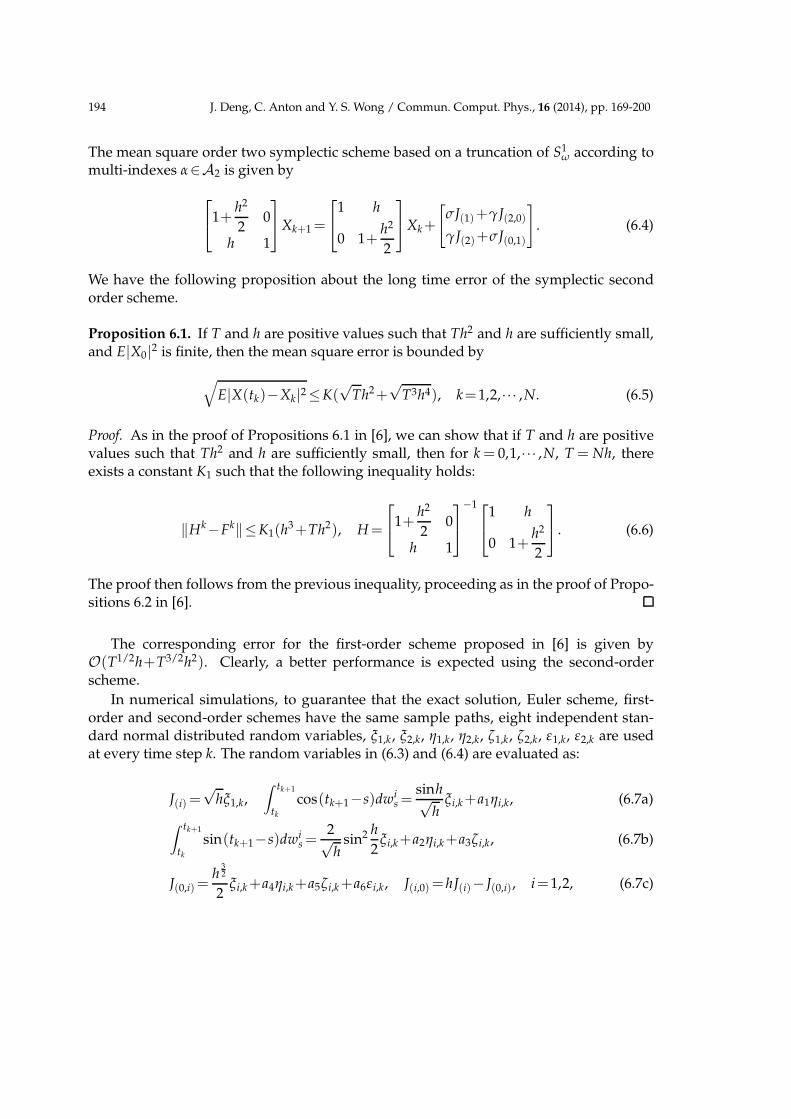
Figure 1: A sample trajectory of the solution to (6.1) for σ= 0, τ= 1, p= 1 and q= 0: exact solution (solid
line), S1ω second order scheme with time step h=2−6 (circle). The circle of different scheme are plotted once
per 10 steps.
−11.5 −11 −10.5 −10 −9.5 −9 −8.5 −8 −7.5 −7 −6.5
−14
−12
−10
−8
−6
−4
−2
log2(h)
log 2(E
rror
)
Order 1.0 sympletic schemeOrder 1.0 reference lineOrder 2.0 sympletic schemeOrder 2.0 reference line
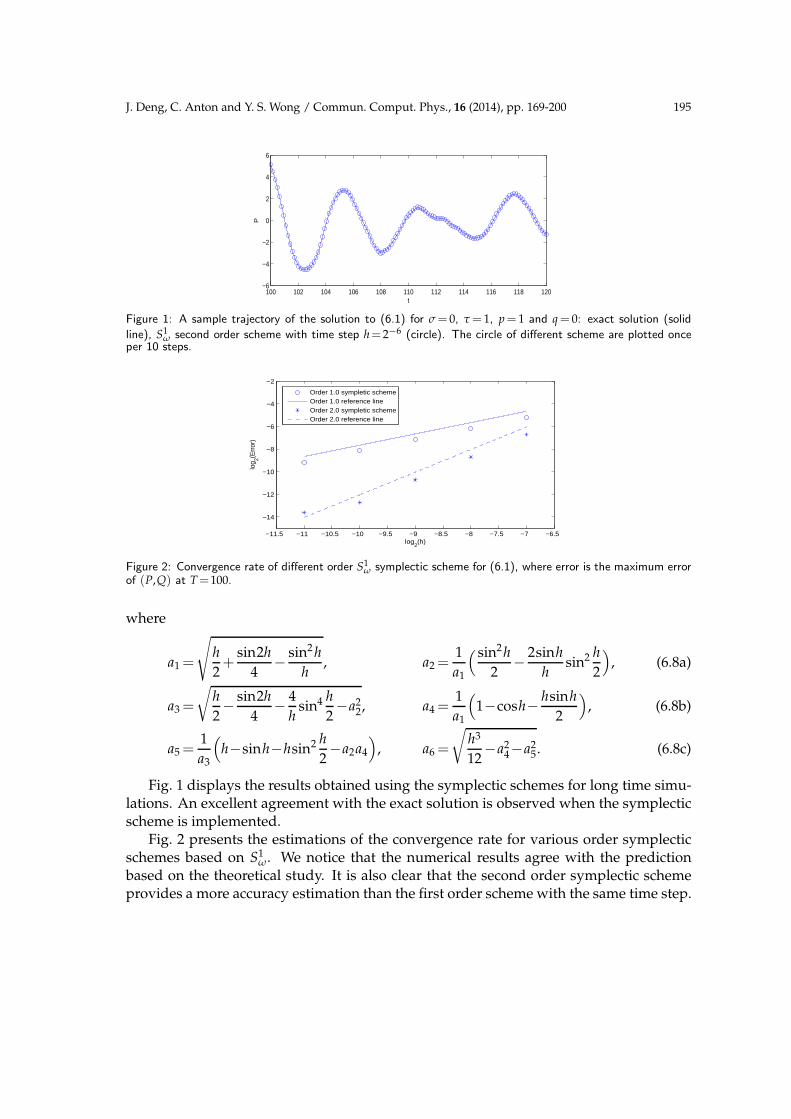
Figure 2: Convergence rate of different order S1ω symplectic scheme for (6.1), where error is the maximum error
of (P,Q) at T=100.
where
a1 =
√
h
2+
sin2h
4− sin2 h
h, a2 =
1
a1
( sin2h
2− 2sinh
hsin2 h
2
)
, (6.8a)
a3 =
√
h
2− sin2h
4− 4
hsin4 h
2−a2
2, a4 =1
a1
(
1−cosh− hsinh
2
)
, (6.8b)
a5 =1
a3
(
h−sinh−hsin2 h
2−a2a4
)
, a6 =
√
h3
12−a2
4−a25. (6.8c)
Fig. 1 displays the results obtained using the symplectic schemes for long time simu-lations. An excellent agreement with the exact solution is observed when the symplecticscheme is implemented.
Fig. 2 presents the estimations of the convergence rate for various order symplecticschemes based on S1
ω. We notice that the numerical results agree with the predictionbased on the theoretical study. It is also clear that the second order symplectic schemeprovides a more accuracy estimation than the first order scheme with the same time step.
196 J. Deng, C. Anton and Y. S. Wong / Commun. Comput. Phys., 16 (2014), pp. 169-200
6.2 Kubo oscillator
In [8], the following SDEs (the Kubo oscillator) in the sense of Stratonovich are used todemonstrate the advantage of the stochastic symplectic scheme for long time computa-tion.
dP=−aQdt−σQ◦dwt , P(0)= p, (6.9a)
dQ= aPdt+σP◦dwt , Q(0)=q, (6.9b)
where a and σ are constants.As illustrated in [8], the Hamiltonian functions
H(0)(P(t),Q(t))= aP(t)2+Q(t)2
2and H(1)(P(t),Q(t))=σ
P(t)2+Q(t)2
2
are preserved under the phase flow of the systems. This means that the phase trajectoryof (6.9) lies on the circle with the center at the origin and the radius
√
p2+q2.Here, we consider the explicit Milstein first order scheme given in (4.24), and five
stochastic symplectic schemes: the mean square 0.5, first and second order schemes basedon S1
ω, and the mean square first- and second-order schemes based on S3ω. The coefficients
G1α of S1
ω for the system (6.9) are given by:
G1(0)=
a
2(p2+q2), G1
(1)=σ
2(p2+q2), G1
(0,0)= a2 pq, G1(1,1)=σ2 pq, (6.10a)
G1(1,0)=G1
(0,1)= aσpq, G1(0,0,0)= a3(p2+q2), G1
(1,1,1)=σ3(p2+q2), (6.10b)
G1(1,1,0)=G1
(1,0,1)=G1(0,1,1)= aσ2(p2+q2), G1
(1,1,1,1)=5σ4 pq. (6.10c)
The various order symplectic schemes are obtained by truncating the generating functionS1
ω appropriately (see (5.14)) for the second order scheme).For S3
ω, G3α for SHSs preserving Hamiltonian functions is zero when l(α)=2,4. Thus
G3(0)=
a
2(p2+q2), G3
(1)=σ
2(p2+q2), G3
(0,0,0)=a3
4(p2+q2), (6.11a)
G3(1,1,1)=
σ3
4(p2+q2), G3
(1,1,0)=G3(1,0,1)=G3
(0,1,1)
aσ2
4(p2+q2). (6.11b)
The first-order midpoint scheme was already applied in [8] for the system (6.9) to illus-trate the superior performance on the long time intervals compared to the non-symplecticschemes. The second-order midpoint scheme is given in (5.14).
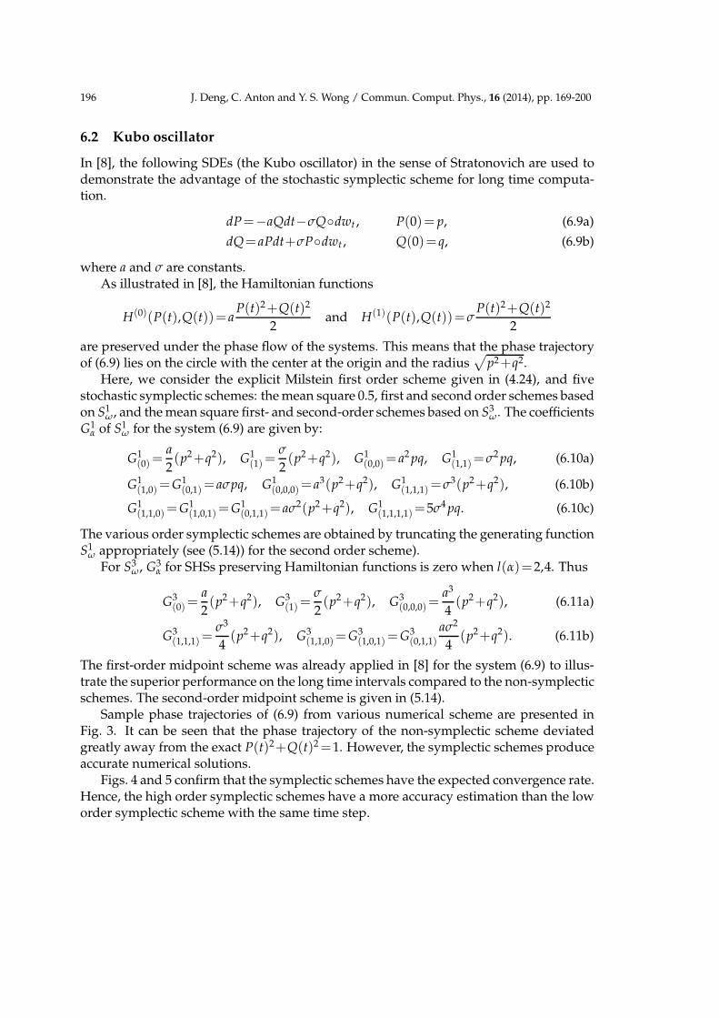
Sample phase trajectories of (6.9) from various numerical scheme are presented inFig. 3. It can be seen that the phase trajectory of the non-symplectic scheme deviatedgreatly away from the exact P(t)2+Q(t)2=1. However, the symplectic schemes produceaccurate numerical solutions.
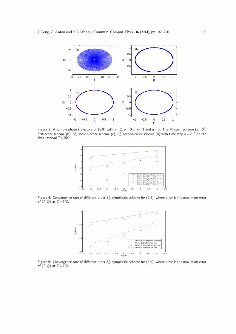
Figs. 4 and 5 confirm that the symplectic schemes have the expected convergence rate.Hence, the high order symplectic schemes have a more accuracy estimation than the loworder symplectic scheme with the same time step.
J. Deng, C. Anton and Y. S. Wong / Commun. Comput. Phys., 16 (2014), pp. 169-200 197
−30 −20 −10 0 10 20 30
−20
0
20
P
Q
−1 −0.5 0 0.5 1
−1
−0.5
0
0.5
1
P
Q−1 −0.5 0 0.5 1
−1
−0.5
0
0.5
1
P
Q
−1 −0.5 0 0.5 1
−1
−0.5
0
0.5
1
PQ
(a) (b)
(c) (d)
Figure 3: A sample phase trajectory of (6.9) with a=2, σ=0.3, p=1 and q=0: The Milstein scheme (a); S1ω
first-order scheme (b); S1ω second-order scheme (c); S3
ω second-order scheme (d) with time step h=2−8 on thetime interval T≤200.
−12.5 −12 −11.5 −11 −10.5 −10 −9.5 −9 −8.5 −8 −7.5
−16
−14
−12
−10
−8
−6
−4
log2(h)
log2(E
rror)
Order 0.5 sympletic schemeOrder 0.5 reference lineOrder 1.0 sympletic schemeOrder 1.0 reference lineOrder 2.0 sympletic schemeOrder 2.0 reference line
Figure 4: Convergence rate of different order S1ω symplectic scheme for (6.9), where error is the maximum error
of (P,Q) at T=100.
−12.5 −12 −11.5 −11 −10.5 −10 −9.5 −9 −8.5 −8 −7.5−20
−15
−10
−5
log2(h)
log 2(E
rror)
Order 1.0 sympletic schemeOrder 1.0 reference lineOrder 2.0 sympletic schemeOrder 2.0 reference line
Figure 5: Convergence rate of different order S3ω symplectic scheme for (6.9), where error is the maximum error
of (P,Q) at T=100.
198 J. Deng, C. Anton and Y. S. Wong / Commun. Comput. Phys., 16 (2014), pp. 169-200
2.8 3 3.2 3.4 3.6 3.8 4 4.2 4.4 4.6−4.5
−4
−3.5
−3
−2.5
−2
−1.5
−1
−0.5
0
0.5
log10
(computational time) (s)
log 10
(err
or)
Milstein Symplectic Order 0.5Symplectic Order 1.0Symplectic Order 2.0
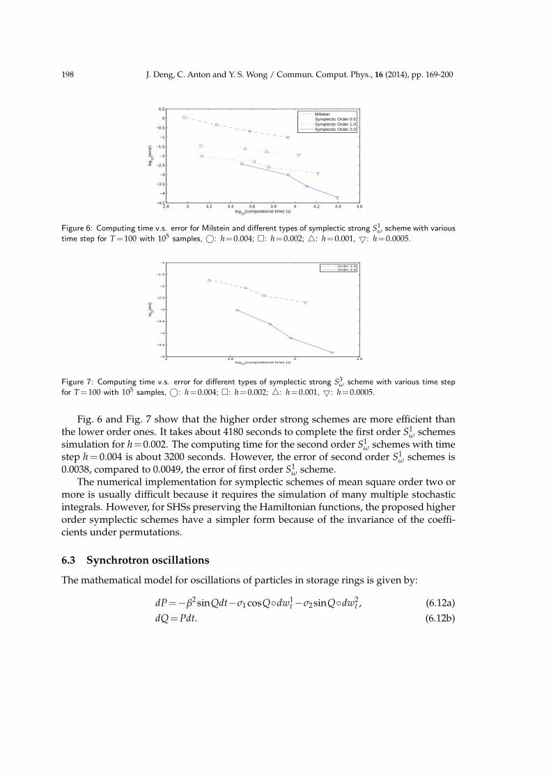
Figure 6: Computing time v.s. error for Milstein and different types of symplectic strong S1ω scheme with various
time step for T=100 with 105 samples, ©: h=0.004; �: h=0.002; △: h=0.001, ▽: h=0.0005.
3 3.5 4 4.5−5
−4.5
−4
−3.5
−3
−2.5
−2
−1.5
−1
log10
(computational time) (s)
log10
(error
)
Order 1.0Order 2.0
Figure 7: Computing time v.s. error for different types of symplectic strong S3ω scheme with various time step
for T=100 with 105 samples, ©: h=0.004; �: h=0.002; △: h=0.001, ▽: h=0.0005.
Fig. 6 and Fig. 7 show that the higher order strong schemes are more efficient thanthe lower order ones. It takes about 4180 seconds to complete the first order S1
ω schemessimulation for h=0.002. The computing time for the second order S1
ω schemes with timestep h= 0.004 is about 3200 seconds. However, the error of second order S1
ω schemes is0.0038, compared to 0.0049, the error of first order S1
ω scheme.The numerical implementation for symplectic schemes of mean square order two or
more is usually difficult because it requires the simulation of many multiple stochasticintegrals. However, for SHSs preserving the Hamiltonian functions, the proposed higherorder symplectic schemes have a simpler form because of the invariance of the coeffi-cients under permutations.
6.3 Synchrotron oscillations
The mathematical model for oscillations of particles in storage rings is given by:
dP=−β2sinQdt−σ1 cosQ◦dw1t −σ2sinQ◦dw2
t , (6.12a)
dQ=Pdt. (6.12b)
J. Deng, C. Anton and Y. S. Wong / Commun. Comput. Phys., 16 (2014), pp. 169-200 199
0 10 20 30 40 50 60 70 80 90 100−1.5
−1
−0.5
0
0.5
1
1.5
2
t
P
Sω1 1.5 order scheme
Sω1 1.0 order scheme
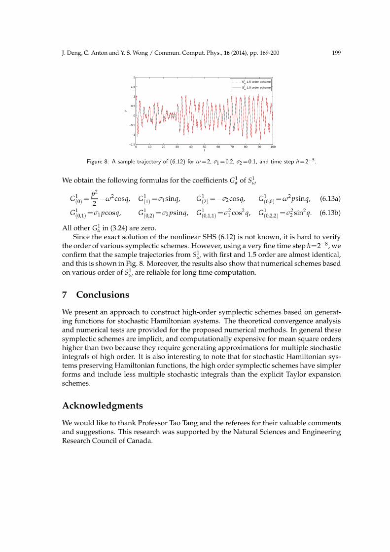
Figure 8: A sample trajectory of (6.12) for ω=2, σ1 =0.2, σ2=0.1, and time step h=2−5.
We obtain the following formulas for the coefficients G1α of S1
ω
G1(0)=
p2
2−ω2cosq, G1
(1)=σ1sinq, G1(2)=−σ2cosq, G1
(0,0)=ω2psinq, (6.13a)
G1(0,1)=σ1 pcosq, G1
(0,2)=σ2 psinq, G1(0,1,1)=σ2
1 cos2 q, G1(0,2,2)=σ2
2 sin2q. (6.13b)
All other G1α in (3.24) are zero.
Since the exact solution of the nonlinear SHS (6.12) is not known, it is hard to verifythe order of various symplectic schemes. However, using a very fine time step h=2−8, weconfirm that the sample trajectories from S1
ω with first and 1.5 order are almost identical,and this is shown in Fig. 8. Moreover, the results also show that numerical schemes basedon various order of S1
ω are reliable for long time computation.
7 Conclusions
We present an approach to construct high-order symplectic schemes based on generat-ing functions for stochastic Hamiltonian systems. The theoretical convergence analysisand numerical tests are provided for the proposed numerical methods. In general thesesymplectic schemes are implicit, and computationally expensive for mean square ordershigher than two because they require generating approximations for multiple stochasticintegrals of high order. It is also interesting to note that for stochastic Hamiltonian sys-tems preserving Hamiltonian functions, the high order symplectic schemes have simplerforms and include less multiple stochastic integrals than the explicit Taylor expansionschemes.
Acknowledgments
We would like to thank Professor Tao Tang and the referees for their valuable commentsand suggestions. This research was supported by the Natural Sciences and EngineeringResearch Council of Canada.
200 J. Deng, C. Anton and Y. S. Wong / Commun. Comput. Phys., 16 (2014), pp. 169-200
References
[1] R. de Vogelaere, Methods of integration which preserve the contact transformation propertyof the hamiltonian equations, Tech. Rep., Report No. 4, Dept. Math., Univ. of Notre Dame,Notre Dame, Ind., (1956).
[2] R. Ruth, A canonical integration technique, IEEE Trans. Nuclear Sci., 30 (1983), 2669–2671.[3] K. Feng, On difference schemes and symplectic geometry, in: Proceedings of the 5-th Intern,
Symposium on Differential Geometry & Differential Equations, Beijing, China, 1985, 42–58.[4] X. Liu, Y. Qi, J. He and P. Ding, Recent progress in symplectic algorithms for use in quantum
systems, Commun. Comput. Phys., 2(1) (2007), 1–53.[5] J. Hong, S. Jiang, C. Li and H. Liu, Explicit multi-symplectic methods for Hamiltonian wave
equations, Commun. Comput. Phys., 2 (2007), 662–683.[6] G. N. Milstein, M. V. Tretyakov and Y. M. Repin, Symplectic integration of hamiltonian sys-
tems with additive noise, SIAM J. Numer. Anal., 39 (2002), 2066–2088.[7] H. Kunita, Stochastic Flows and Stochastic Differential Equations, Cambridge University
Press, 1990.[8] G. N. Milstein, M. V. Tretyakov and Y. M. Repin, Numerical methods for stochastic systems
preserving symplectic structure, SIAM J. Numer. Anal., 40 (2002), 1583–1604.[9] J. Hong, R. Scherer and L. Wang, Predictorcorrector methods for a linear stochastic oscillator
with additive noise, Math. Comput. Model., 46(5-6) (2007), 738–764.[10] A. Melbo and D. Higham, Numerical simulation of a linear stochastic oscillator with addi-
tive noise, Appl. Numer. Math., 51(1) (2004), 89–99.[11] L. Wang, J. Hong, R. Scherer and F. Bai, Dynamics and variational integrators of stochastic
Hamiltonian systems, Int. J. Numer. Anal. Model., 6(4) (2009), 586–602.[12] J. Hong, L. Wang and R. Scherer, Simulation of stochastic Hamiltonian systems via generat-
ing functions, in: Proceedings IEEE 2011 4th ICCSIT, 2011.[13] J. Hong, L. Wang and R. Scherer, Symplectic numerical methods for a linear stochastic oscil-
lator with two additive noises, in: Proceedings of the World Congress on Engineering, Vol.I, London, U.K., 2011.
[14] L. Wang. Variational integrators and generating functions for stochastic Hamiltonian sys-tems, KIT Scientific Publishing, University of Karlsruhe, Germany, 2007, Dissertation,www.ksp.kit.edu.
[15] J.-M. Bismut and Mecanique Aleatoire, Lecture Notes in Mathematics, Vol. 866, Springer-Verlag, Berlin-Heidelberg-New York, 1981.
[16] E. Hairer, Geometric Numerical Integration: Structure-Preserving Algorithms for OrdinaryDifferential Equations, Springer, Berlin, New York, 2006.
[17] K. Feng, H. Wu, M. Qin and D. Wang, Construction of canonical difference schemes forHamiltonian formalism via generating functions, J. Comput. Math., 7 (1989), 71–96.
[18] C. Anton, J. Deng and Y. S. Wong, Weak symplectic schemes for stochastic Hamiltonianequations, Electronic Transactions on Numerical Analysis, to appear.
[19] P. Kloeden and E. Platen, Numerical Solutions of Stochastic Differential Equations, Springer-Verlag, Berlin, 1992.
[20] G. N. Milstein, Numerical Integration of Stochastic Differential Equations, Kluwer Aca-demic Publishers, Dordrecht, Boston, 1995.
[21] C. Anton, Y. S. Wong and J. Deng, Symplectic schemes for stochastic Hamiltonian systemspreserving Hamiltonian functions, Int. J. Numer. Anal. Model., 11(3) (2014), 427–451.