SYMMETRICAL OPTIMUM BASED PI CONTROL REDESIGN · SYMMETRICAL OPTIMUM BASED PI CONTROL REDESIGN ... (Voda and Landau, ... Anais do XX Congresso Brasileiro de Automática

SYMMETRICAL OPTIMUM BASED PI CONTROL REDESIGN

Andre L. S. Barbosa∗ George Acioli Junior∗ Pericles R. Barros∗

∗Departamento de Engenharia EletricaUniversidade Federal de Campina Grande

Campina Grande, Paraıba, Brasil

Email: [email protected] [email protected]

[email protected]

Abstract— In this paper a proposal for redesign PI controllers with Symmetrical Optimum (SO) based designis presented. The method, introduced by the authors and called Modified Symmetrical Optimum (MSO), uses anintegration plus first-order model, identified from two frequency points obtained from combined relay experiment.The proposal for the identification of the used model is also presented. The MSO idea is to apply a parameterizedSO method to get a controller with stability and robustness aspects. The results analysis is performed bysimulation examples.

Keywords— Controller design, Stability analysis, PI Controllers, System identification, Relay experiment.

Resumo— Neste trabalho, e apresentada uma proposta de reprojeto para controladores PI baseada em controleOtimo Simetrico (SO). O metodo, introduzido pelos autores e chamado de Otimo Simetrico Modificado (MSO),utiliza um modelo de primeira ordem mais um integrador, identificado a partir de dois pontos em frequenciaobtidos com um experimento combinado do rele. A proposta para a identificacao deste modelo utilizado tambeme apresentada. A ideia do MSO e aplicar o SO com uma parametrizacao para se conseguir um controlador comaspectos relacionados a estabilidade e robustez do sistema. A analise dos resultados e realizada por meio deexemplos de simulacoes.

Palavras-chave— Projeto de controladores, Analise de estabilidade, Controladores PI, Identificacao de siste-mas, Experimento do rele.

1 Introduction

The PID controller is the most common solutionto practical control problems. This can be at-tributed to its robust performance and simplicityto get the tuning parameters. Depending on thedynamics of the process and the way that the con-troller is being applied, the task to get the threecontroller parameters can not be so simple. Fur-thermore, it is necessary to choose among the var-ious existing tuning techniques to obtain the de-sired performance. In the industrial environment,in most cases, there is not much information aboutthe dynamics of the process, which can complicatethe control design. To perform an experiment toget the plant by mathematical models becomes analternative to adjust the parameters of control de-sign.

Among the contributions in tuning PID con-trollers, (Ziegler and Nichols, 1942) is the majorreference. Over time, several modifications to theoriginal experiment appeared in order to improvedifferent aspects of the project. (Astrom and Hag-glund, 1984) have presented the tuning of PI andPID controllers based on the identification of thefrequency response to obtain the gain and phasemargins of the process plant. The relay experi-ment was modified later in (Leva, 1993) with theintroduction of a variable delay in the loop in orderto obtain different information of the frequency re-sponse of the process.

From the viewpoint of PID tuning, other stud-ies are rather quoted in the literature. (Kessler,

1958) has presented the concept of SymmetricalOptimum Method (SO). In this context, the pro-cess is reduced to a model that assumes integra-tors plus fast dynamics (small time constants anddelays) captured by a single parameter to resultin a slope with −20dB/dec in the bode plot infrequency response close to crossover frequency.With the simplicity of the method, (Voda andLandau, 1995) have showed a SO expansion witha calibration method called PID controller tuningrules KLV (Kessler-Landau-Voda). The method,combined with the relay experiments, has the ad-vantage of robustness in many respects in the fre-quency domain. The controller can be adjustedby simple tuning rules with guaranteed stabil-ity and robustness from information obtained inthe frequency −135◦. Still with the SO, thereare recent studies. (Preitl and Precup, 1999)and (Preitl et al., 2011) have implemented exten-sions and parameterization of the original method.(Papadopoulos et al., 2011) with extension in(Papadopoulos et al., 2012) have showed the prin-ciples of their application that aims to tune PIDcontroller for the final output of the closed loopsystem results in the elimination of higher-order,position, velocity and acceleration errors and oth-ers control strategies.

This paper treats the use of SO for tuning PIcontrollers, aiming to obtain a stable controllerfor several classes of processes. The paper is or-ganized as follows: in Section 2 the problem isformulated; a brief summary of SO is presented

Anais do XX Congresso Brasileiro de Automática Belo Horizonte, MG, 20 a 24 de Setembro de 2014

1143

in Section 3; in Section 4 is shown the identifi-cation procedure and controller tuning, the sta-bility analysis of the standard method and theproposed redesign to obtain a stable controller isshown in Section 5; in Section 6 is presented themodified SO PI controller; simulation and exam-ples are shown in Section 7.

2 The Problem Statement

Consider the process G(s) with unknown dy-namic. The process model transfer function G(s)is represented by the following model

G(s) =K

′

s(TΣs+ 1), (1)

where the gain K′ and time constant TΣ are esti-

mated parameters. The PI controller used is givenby

C(s) = Kp

(

1 +1

Tis

)

. (2)

Assume that the PI controller C (s) was de-signed using the estimated model G(s) and the SObased design. For processes which such a modelG(s) is not a good approximation, the robustnessproperties of the SO can be lost.

The problem statement is: given a processG(s), important information about the processcan be obtained using relay experiments, includingthe process model G(s). Using these information,the designed SO controller based on the modelG(s) is evaluated using the experimental data andmodified SO based controller is suggested.

3 The Symmetrical Optimum Design

In the method introduced by (Kessler, 1958), theprocess to be controlled is considered as follows:

G(s) =K

(TΣs+ 1)m∏

k=1

(Tks+ 1), (3)

where Tk are the plant’s dominant time constants,TΣ represents the sum of all the process parasiticstime constants (fast time constants plus delay).For PI and PID controllers, m = 1 and m = 2respectively.

Consider Tk ≫ TΣ. In the region close tothe crossover frequency of the system, an ap-proximated model can be obtained by a cascadeof pure integrators (1/(1 + sTk) ≈ 1/sTk) for(ω ≈ 1/(2TΣ)).

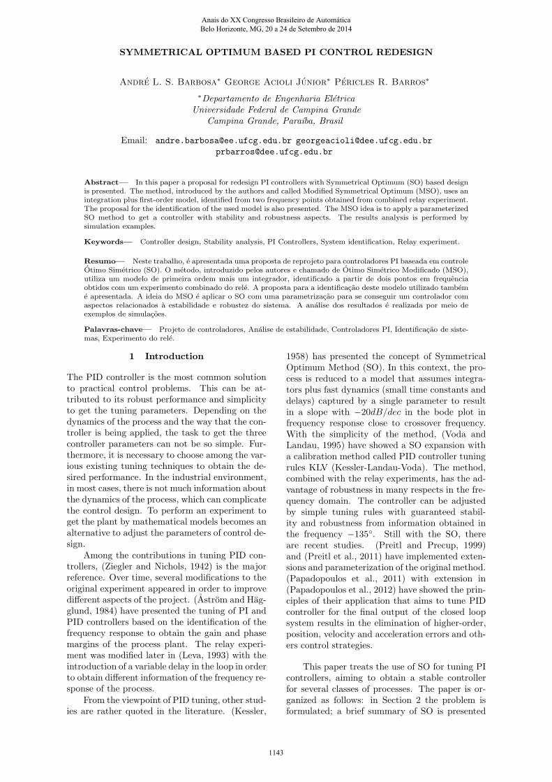
This technique has the advantage of robust-ness in various aspects (phase margin, gain mar-gin, sensitivity and processes dynamics). In Fig. 1is illustrated the Bode Diagram of the open looptransfer function for SO method. When captur-ing all the fast dynamics of the system in a single

pole, as described in (3), this pole is used as a lim-iting factor for the crossover frequency resultingin a closed loop with a certain stability margin.More information about SO see (Kessler, 1958)and (Voda and Landau, 1995).

L

Figure 1: Bode Diagram with SO based design forPI (m = 1) and PID (m = 2) controllers

For PI controllers, the model used is

G(s) =K

T1s(TΣs+ 1)(4)

and the parallel PI tuning rules are Kp =12 (

T1

K)( 1

TΣ) and Ti = 4TΣ.

In the next Section it will be discussed how toexperimentally obtain such a model.

4 Model Identification

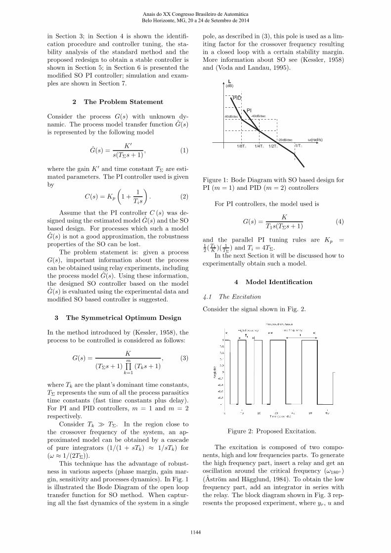
4.1 The Excitation

Consider the signal shown in Fig. 2.

Figure 2: Proposed Excitation.

The excitation is composed of two compo-nents, high and low frequencies parts. To generatethe high frequency part, insert a relay and get anoscillation around the critical frequency (ω180◦)

(Astrom and Hagglund, 1984). To obtain the lowfrequency part, add an integrator in series withthe relay. The block diagram shown in Fig. 3 rep-resents the proposed experiment, where yr, u and


1144

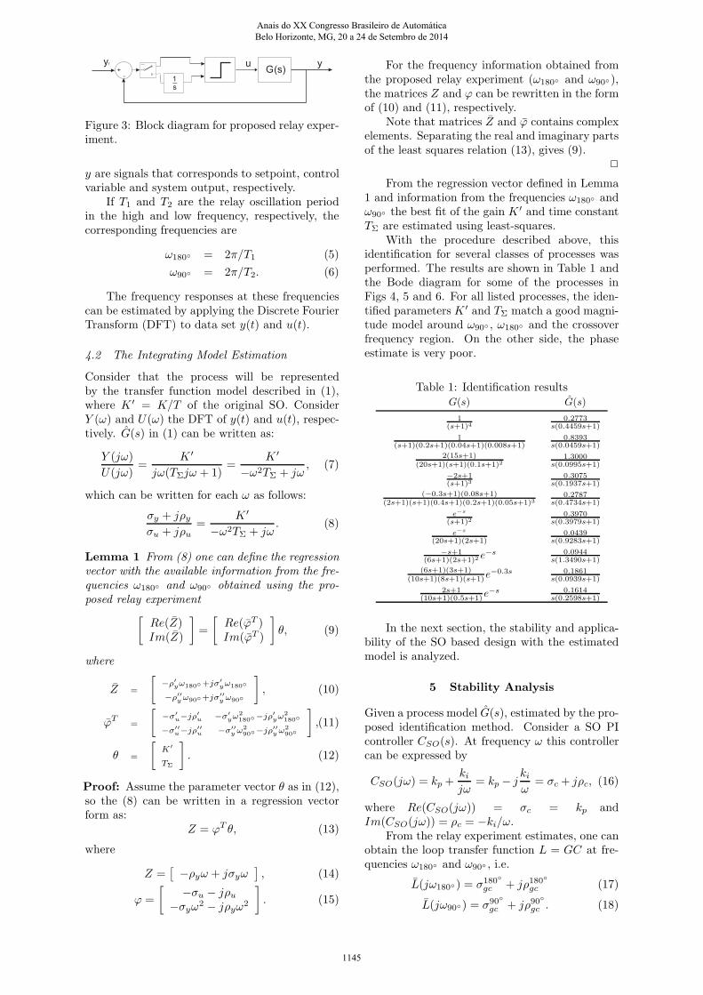
Figure 3: Block diagram for proposed relay exper-iment.

y are signals that corresponds to setpoint, controlvariable and system output, respectively.

If T1 and T2 are the relay oscillation periodin the high and low frequency, respectively, thecorresponding frequencies are

ω180◦ = 2π/T1 (5)

ω90◦ = 2π/T2. (6)

The frequency responses at these frequenciescan be estimated by applying the Discrete FourierTransform (DFT) to data set y(t) and u(t).

4.2 The Integrating Model Estimation

Consider that the process will be representedby the transfer function model described in (1),where K

′ = K/T of the original SO. ConsiderY (ω) and U(ω) the DFT of y(t) and u(t), respec-tively. G(s) in (1) can be written as:

Y (jω)

U(jω)=

K′

jω(TΣjω + 1)=

K′

−ω2TΣ + jω

, (7)

which can be written for each ω as follows:

σy + jρy

σu + jρu

=K

′

−ω2TΣ + jω

. (8)

Lemma 1 From (8) one can define the regressionvector with the available information from the fre-quencies ω180◦ and ω90◦ obtained using the pro-posed relay experiment

[

Re(Z)Im(Z)

]

=

[

Re(ϕT )Im(ϕT )

]

θ, (9)

where

Z =

[

−ρ′

yω180◦+jσ′

yω180◦

−ρ′′

yω90◦+jσ′′

yω90◦

]

, (10)

ϕT

=

[

−σ′

u−jρ′

u−σ′

yω2

180◦−jρ′

yω2

180◦

−σ′′

u−jρ′′

u−σ′′

yω2

90◦−jρ′′

yω2

90◦

]

,(11)

θ =

[

K′

TΣ

]

. (12)

Proof: Assume the parameter vector θ as in (12),so the (8) can be written in a regression vectorform as:

Z = ϕTθ, (13)

where

Z =[

−ρyω + jσyω

]

, (14)

ϕ =

[

−σu − jρu

−σyω2− jρyω

2

]

. (15)

For the frequency information obtained fromthe proposed relay experiment (ω180◦ and ω90◦),the matrices Z and ϕ can be rewritten in the formof (10) and (11), respectively.

Note that matrices Z and ϕ contains complexelements. Separating the real and imaginary partsof the least squares relation (13), gives (9).

✷

From the regression vector defined in Lemma1 and information from the frequencies ω180◦ andω90◦ the best fit of the gain K

′ and time constantTΣ are estimated using least-squares.

With the procedure described above, thisidentification for several classes of processes wasperformed. The results are shown in Table 1 andthe Bode diagram for some of the processes inFigs 4, 5 and 6. For all listed processes, the iden-tified parameters K ′ and TΣ match a good magni-tude model around ω90◦ , ω180◦ and the crossoverfrequency region. On the other side, the phaseestimate is very poor.

Table 1: Identification resultsG(s) G(s)

1(s+1)4

0.2773s(0.4459s+1)

1(s+1)(0.2s+1)(0.04s+1)(0.008s+1)

0.8393s(0.0459s+1)

2(15s+1)(20s+1)(s+1)(0.1s+1)2

1.3000s(0.0995s+1)

−2s+1(s+1)3

0.3075s(0.1937s+1)

(−0.3s+1)(0.08s+1)(2s+1)(s+1)(0.4s+1)(0.2s+1)(0.05s+1)3

0.2787s(0.4734s+1)

e−s

(s+1)20.3970

s(0.3979s+1)

e−s

(20s+1)(2s+1)0.0439

s(0.9283s+1)

−s+1(6s+1)(2s+1)2 e

−s 0.0944s(1.3490s+1)

(6s+1)(3s+1)(10s+1)(8s+1)(s+1)e

−0.3s 0.1861s(0.0939s+1)

2s+1(10s+1)(0.5s+1)e

−s 0.1614s(0.2598s+1)

In the next section, the stability and applica-bility of the SO based design with the estimatedmodel is analyzed.

5 Stability Analysis

Given a process model G(s), estimated by the pro-posed identification method. Consider a SO PIcontroller CSO(s). At frequency ω this controllercan be expressed by

CSO(jω) = kp +ki

jω

= kp − j

ki

ω

= σc + jρc, (16)

where Re(CSO(jω)) = σc = kp andIm(CSO(jω)) = ρc = −ki/ω.

From the relay experiment estimates, one canobtain the loop transfer function L = GC at fre-quencies ω180◦ and ω90◦ , i.e.

L(jω180◦) = σ180◦

gc + jρ180◦

gc (17)

L(jω90◦) = σ90◦

gc + jρ90◦

gc . (18)


1145

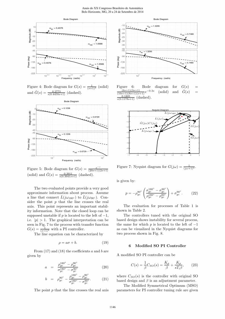
Figure 4: Bode diagram for G(s) = 1(s+1)4 (solid)

and G(s) = 0.2773s(0.4459s+1) (dashed).

Figure 5: Bode diagram for G(s) = e−s

(20s+1)(2s+1)

(solid) and G(s) = 0.3911s(0.3941s+1) (dashed).

The two evaluated points provide a very goodapproximate information about process. Assumea line that connect L(jω180◦) to L(jω90◦). Con-sider the point p that the line crosses the realaxis. This point represents an important stabil-ity information. Note that the closed loop can besupposed unstable if p is located to the left of −1,i.e. |p| > 1. The graphical interpretation can beseen in Fig. 7 to the process with transfer functionG(s) = 1

(s+1)4 with a PI controller.

The line equation can be characterized by

ρ = aσ + b. (19)

From (17) and (18) the coefficients a and b aregiven by

a =ρ180◦

gc − ρ90◦

gc

σ180◦gc − σ

90◦gc

(20)

b = ρ90◦

gc −

ρ180◦

gc − ρ90◦

gc

σ180◦gc − σ

90◦gc

. (21)

The point p that the line crosses the real axis

Figure 6: Bode diagram for G(s) =(6s+1)(3s+1)

(10s+1)(8s+1)(s+1)e−0.3s (solid) and G(s) =

0.1805s(0.1178s+1) (dashed).

Nyquist Diagram

−7 −6 −5 −4 −3 −2 −1 0 1−7

−6

−5

−4

−3

−2

−1

0

1

G(jω)C(jω)

L(jω180◦ )

L(jω90◦ )

L(jω) p

G(jω)

G(jω)

Figure 7: Nyquist diagram for G(jω) = 1(jω+1)4 .

is given by:

p = −ρ90◦

gc

(

σ180◦

gc − σ90◦

gc

ρ180◦gc − ρ

90◦gc

)

+ σ90◦

gc . (22)

The evaluation for processes of Table 1 isshown in Table 2.

The controllers tuned with the original SObased design shows instability for several process,the same for which p is located to the left of −1as can be visualized in the Nyquist diagrams fortwo process shown in Fig. 8.

6 Modified SO PI Controller

A modified SO PI controller can be

C(s) =1

β

CSO(s) =Kp

β

+Kp

sTiβ, (23)

where CSO(s) is the controller with original SObased design and β is an adjustment parameter.

The Modified Symmetrical Optimum (MSO)parameters for PI controller tuning rule are given


1146

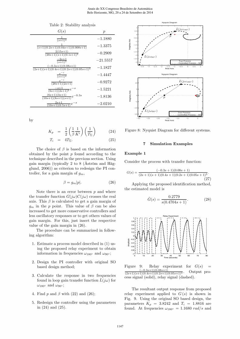
Table 2: Stability analysis

G(s) p

1(s+1)4 −1.1880

1(s+1)(0.2s+1)(0.04s+1)(0.008s+1) −1.3375

2(15s+1)(20s+1)(s+1)(0.1s+1)2 −0.2909

−2s+1(s+1)3 −21.5557

(−0.3s+1)(0.08s+1)(2s+1)(s+1)(0.4s+1)(0.2s+1)(0.05s+1)3 −1.1827

e−s

(s+1)2 −1.4447

e−s

(20s+1)(2s+1) −0.9272

−s+1(6s+1)(2s+1)2 e

−s−1.5221

(6s+1)(3s+1)(10s+1)(8s+1)(s+1)e

−0.3s−1.8136

2s+1(10s+1)(0.5s+1)e

−s−2.0210

by

Kp =1

2

(

1

β

1

K′

)(

1

TΣ

)

(24)

Ti = 4TΣ. (25)

The choice of β is based on the informationobtained by the point p found according to thetechnique described in the previous section. Usinggain margin (typically 2 to 8 (Astrom and Hag-glund, 2006)) as criterion to redesign the PI con-troller, for a gain margin of gm,

β = gm|p|. (26)

Note there is an error between p and wherethe transfer function G(jω)C(jω) crosses the realaxis. This β is calculated to get a gain margin ofgm in the p point. This value of β can be alsoincreased to get more conservative controllers andless oscillatory responses or to get others values ofgain margin. For this, just insert the respectivevalue of the gain margin in (26).

The procedure can be summarized in follow-ing algorithm:

1. Estimate a process model described in (1) us-ing the proposed relay experiment to obtaininformation in frequencies ω180◦ and ω90◦ ;

2. Design the PI controller with original SObased design method;

3. Calculate the response in two frequenciesfound in loop gain transfer function L(jω) forω180◦ and ω90◦ ;

4. Find p and β with (22) and (26);

5. Redesign the controller using the parametersin (24) and (25).

Nyquist Diagram

Real Axis

Imag

inar

y Ax

is

−3.5 −3 −2.5 −2 −1.5 −1 −0.5 0 0.5 1

−4

−3.5

−3

−2.5

−2

−1.5

−1

−0.5

0

0.5

1

True ProcessControlled Process − SO

L(jω180◦)

L(jω90◦)

p

Nyquist Diagram

Real Axis

Imag

inar

y Ax

is

−30 −25 −20 −15 −10 −5 0

−15

−10

−5

0

5

10

True ProcessControlled Process − SO

p

L(jω90◦)

L(jω180◦)

Figure 8: Nyquist Diagram for different systems.

7 Simulation Examples

Example 1

Consider the process with transfer function:

G(s) =(−0.3s+ 1)(0.08s + 1)

(2s+ 1)(s + 1)(0.4s+ 1)(0.2s+ 1)(0.05s + 1)3.

(27)

Applying the proposed identification method,the estimated model is

G(s) =0.2779

s(0.4704s+ 1). (28)

Figure 9: Relay experiment for G(s) =(−0.3s+1)(0.08s+1)

(2s+1)(s+1)(0.4s+1)(0.2s+1)(0.05s+1)3 . Output pro-

cess signal (solid), relay signal (dashed).

The resultant output response from proposedrelay experiment applied to G (s) is shown inFig. 9. Using the original SO based design, theparameters Kp = 3.8242 and Ti = 1.8816 arefound. At frequencies ω180◦ = 1.1680 rad/s and


1147

ω90◦ = 0.4323 rad/s, L(jω) can be found:

L(jω180◦) = −0.8942 + j0.4129 (29)

L(jω90◦) = −3.1704− j2.7224. (30)

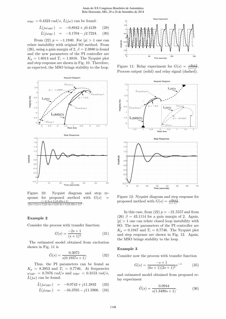
From (22) p = −1.1940. For |p| > 1 one canrelate instability with original SO method. From(26), using a gain margin of 2, β = 2.3880 is foundand the new parameters of the PI controller areKp = 1.6014 and Ti = 1.8816. The Nyquist plotand step response are shown in Fig. 10. Therefore,as expected, the MSO brings stability to the loop.

L(MSO)

L(SO)

Figure 10: Nyquist diagram and step re-sponse for proposed method with G(s) =

(−0.3s+1)(0.08s+1)(2s+1)(s+1)(0.4s+1)(0.2s+1)(0.05s+1)3 .

Example 2

Consider the process with transfer function:

G(s) =−2s+ 1

(s+ 1)3(31)

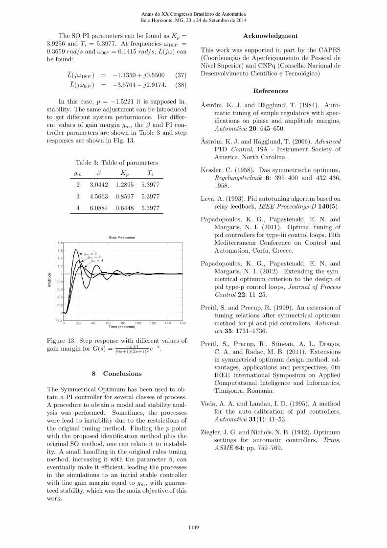
The estimated model obtained from excitationshown in Fig. 11 is

G(s) =0.3075

s(0.1937s+ 1). (32)

Thus, the PI parameters can be found asKp = 8.3953 and Ti = 0.7746. At frequenciesω180◦ = 0.7876 rad/s and ω90◦ = 0.3153 rad/s,L(jω) can be found:

L(jω180◦) = −9.0742 + j11.2833 (33)

L(jω90◦) = −34.3765− j11.5900. (34)

Figure 11: Relay experiment for G(s) = −2s+1(s+1)3 .

Process output (solid) and relay signal (dashed).

L(MSO)

L(SO)

L(SO)

Figure 12: Nyquist diagram and step response forproposed method with G(s) = −2s+1

(s+1)3 .

In this case, from (22) p = −21.5557 and from(26) β = 43.1114 for a gain margin of 2. Again,|p| > 1 one can relate closed loop instability withSO. The new parameters of the PI controller areKp = 0.1947 and Ti = 0.7746. The Nyquist plotand step response are shown in Fig. 12. Again,the MSO brings stability to the loop.

Example 3

Consider now the process with transfer function

G(s) =−s+ 1

(6s+ 1)(2s+ 1)2e−s (35)

and estimated model obtained from proposed re-lay experiment

G(s) =0.0944

s(1.3490s+ 1). (36)


1148

The SO PI parameters can be found as Kp =3.9256 and Ti = 5.3977. At frequencies ω180◦ =0.3659 rad/s and ω90◦ = 0.1415 rad/s, L(jω) canbe found:

L(jω180◦) = −1.1350 + j0.5500 (37)

L(jω90◦) = −3.5764− j2.9174. (38)

In this case, p = −1.5221 it is supposed in-stability. The same adjustment can be introducedto get different system performance. For differ-ent values of gain margin gm, the β and PI con-troller parameters are shown in Table 3 and stepresponses are shown in Fig. 13.

Table 3: Table of parameters

gm β Kp Ti

2 3.0442 1.2895 5.3977

3 4.5663 0.8597 5.3977

4 6.0884 0.6448 5.3977

Figure 13: Step response with different values ofgain margin for G(s) = −s+1

(6s+1)(2s+1)2 e−s.

8 Conclusions

The Symmetrical Optimum has been used to ob-tain a PI controller for several classes of process.A procedure to obtain a model and stability anal-ysis was performed. Sometimes, the processeswere lead to instability due to the restrictions ofthe original tuning method. Finding the p pointwith the proposed identification method plus theoriginal SO method, one can relate it to instabil-ity. A small handling in the original rules tuningmethod, increasing it with the parameter β, caneventually make it efficient, leading the processesin the simulations to an initial stable controllerwith line gain margin equal to gm, with guaran-teed stability, which was the main objective of thiswork.

Acknowledgment

This work was supported in part by the CAPES(Coordenacao de Aperfeicoamento de Pessoal deNıvel Superior) and CNPq (Conselho Nacional deDesenvolvimento Cientıfico e Tecnologico)

References

Astrom, K. J. and Hagglund, T. (1984). Auto-matic tuning of simple regulators with spec-ifications on phase and amplitude margins,Automatica 20: 645–650.

Astrom, K. J. and Hagglund, T. (2006). AdvancedPID Control, ISA - Instrument Society ofAmerica, North Carolina.

Kessler, C. (1958). Das symmetrische optimum,Regelungstechnik 6: 395–400 and 432–436,1958.

Leva, A. (1993). Pid autotuning algoritm based onrelay feedback, IEEE Proceedings-D 140(5).

Papadopoulos, K. G., Papastenaki, E. N. andMargaris, N. I. (2011). Optimal tuning ofpid controllers for type-iii control loops, 19thMediterranean Conference on Control andAutomation, Corfu, Greece.

Papadopoulos, K. G., Papastenaki, E. N. andMargaris, N. I. (2012). Extending the sym-metrical optimum criterion to the design ofpid type-p control loops, Journal of ProcessControl 22: 11–25.

Preitl, S. and Precup, R. (1999). An extension oftuning relations after symmetrical optimummethod for pi and pid controllers, Automat-ica 35: 1731–1736.

Preitl, S., Precup, R., Stınean, A. I., Dragos,C. A. and Radac, M. B. (2011). Extensionsin symmetrical optimum design method. ad-vantages, applications and perspectives, 6thIEEE International Symposium on AppliedComputational Inteligence and Informatics,Timisoara, Romania.

Voda, A. A. and Landau, I. D. (1995). A methodfor the auto-calibration of pid controllers,Automatica 31(1): 41–53.

Ziegler, J. G. and Nichols, N. B. (1942). Optimumsettings for automatic controllers, Trans.ASME 64: pp. 759–769.


1149

Documents

SYMMETRICAL OPTIMUM BASED PI CONTROL REDESIGN · SYMMETRICAL OPTIMUM BASED PI CONTROL REDESIGN ... (Voda and Landau, ... Anais do XX Congresso Brasileiro de Automática