SYMMETRIC SARKISOV LINKS OF FANO THREEFOLDS

SYMMETRIC SARKISOV LINKS OF FANO THREEFOLDS

by

Joseph W. Cutrone

A dissertation submitted to The Johns Hopkins University in conformity with the

requirements for the degree of Doctor of Philosophy.

Baltimore, Maryland

April, 2011

c©Joseph Cutrone 2011

All rights reserved

Abstract

In this thesis, examples of type II Sarkisov links between complex projective Fano

threefolds with Picard number one are provided. To show examples of these links, I

study smooth weak Fano threefolds with Picard number two whose pluri-anticanonical

morphism contracts only a finite number of curves. I focus only on the case when the

Mori extremal contraction of the smooth weak Fano is divisorial and of the same type

both before and after a flop. The numerical classification of these particular types of

smooth weak Fano threefolds with Picard number two is completed and the existence

of some numerical cases is proven.

Readers: Dr. V. Shokurov (Advisor), Dr. S. Zucker, Dr. T. Ono, Dr. P.

Maksimovic, and Dr. C. Herman.

ii

Acknowledgments

I would first like to express my deep gratitude to my advisor, Dr. V.V. Shokurov, for

years of patient guidance.

I would like to especially thank my collaborator, my teacher, and my friend, Nick

Marshburn. I hope I can be as great a math teacher to others as you were to me. May

you buy an adaptor before plugging in a fan in Russia.

I would also like to extend heartfelt thanks to the many graduate students and faculty

at Johns Hopkins who have assisted in ways both large and small throughout this

process: Morris Hunt, Sabrina Raymond, Dr. R. Brown, Dr. J. Kong, Mike Limarzi,

Caleb Hussey, Longzhi Lin, Sinan Artiturk, Steve Kleene, Brian MacDonald, Siddique

Khan, and many others.

I dedicate this dissertation to my family: Mom, Dad, Andrew and Liz. I also dedicate

this dissertation to Anna and Spunkers. Thank you all for your constant love, support,

and cookies.

This thesis was partially supported by NSF grants DMS-0701465 and DMS-1001427.

iii

Contents

Abstract ii

Acknowledgments iii

1 Introduction 1

1.1 Introduction . . . . . . . . . . . . . . . . . . . . . . . . . . . . . . . . . 1

1.2 Definitions and Preliminaries . . . . . . . . . . . . . . . . . . . . . . . . 4

1.3 Prior Results and Background Information . . . . . . . . . . . . . . . . 8

1.4 Assumptions . . . . . . . . . . . . . . . . . . . . . . . . . . . . . . . . . 11

2 Relation to Mori Minimal Model Program 14

2.1 Dimension Three Sarkisov Links . . . . . . . . . . . . . . . . . . . . . . 15

2.1.1 Definition . . . . . . . . . . . . . . . . . . . . . . . . . . . . . . 15

3 E1-E1 Case 17

3.1 Equations and Bounds . . . . . . . . . . . . . . . . . . . . . . . . . . . 17

3.2 Numerical Checks . . . . . . . . . . . . . . . . . . . . . . . . . . . . . . 24

3.3 Elimination of Cases . . . . . . . . . . . . . . . . . . . . . . . . . . . . 26

3.4 Geometric Realization of Cases . . . . . . . . . . . . . . . . . . . . . . 29

4 Non E1-E1 Cases 32

iv

4.1 Numerical Classification . . . . . . . . . . . . . . . . . . . . . . . . . . 32

4.2 Existence of Cases . . . . . . . . . . . . . . . . . . . . . . . . . . . . . 35

5 Tables 37

5.1 E1 - E1 . . . . . . . . . . . . . . . . . . . . . . . . . . . . . . . . . . . 37

5.2 E2 - E2 . . . . . . . . . . . . . . . . . . . . . . . . . . . . . . . . . . . 41

5.3 E3/4 - E3/4 . . . . . . . . . . . . . . . . . . . . . . . . . . . . . . . . . 42

5.4 E5 - E5 . . . . . . . . . . . . . . . . . . . . . . . . . . . . . . . . . . . 43

Appendix: Algorithm Source Code 44

Bibliography 53

Vitae 56

v

Chapter 1

Introduction

1.1 Introduction

The study and classification of weak Fano threefolds is important in the framework

of the Mori minimal model program as well as a branch of algebraic geometry called

Sarkisov theory.

Starting with a Q-factorial variety Y with at most terminal singularities, the end

result of running the Mori minimal model program on Y is either a minimal model or

a Mori fibration. If the canonical divisor KY is nef then Y is defined to be a minimal

model. A Mori fibration (equivalently, a Mori fiber space) is defined as a contraction

φ : Y → S, where S is a normal projective variety such that the relative Picard number

ρ(Y/S) = 1, dim Y > dim S, and −KY is φ-ample. These latter varieties will be our

primary objects of study.

Given a birational map between two threefold Mori fiber spaces, it is natural to ask

whether this map decomposes as a composition of elementary birational morphisms.

Kawamata has shown that any birational map between minimal models of a threefold

decomposes as a finite sequence of flops ([Ka08]). This result is true for higher dimen-

1

sional minimal models as well ([ShC10]). In [Sar89], Sarkisov introduced elementary

links (certain birational maps) between Mori fiber spaces and in [Cor95] Corti proved

that any birational map between threefold Mori fiber spaces is a composition of these

elementary links. In addition, Corti showed that there are only four kinds of links

that can exist, thus completing the Sarkisov program in dimension three. They are

appropriately called links of type I, II, III and IV.

Any Sarkisov link has a central variety. If the link contains a flop, both varieties on

either side of the flop are central varieties. If the link does not contain a flop, the central

variety is unique. Fixing a central variety, there are a series of small modifications (a

flop and flips in both directions) which preserve terminal singularities and Q-factorality,

followed by divisorial or fibered contractions. Sarkisov links will be further explained

in Section 2.1.

I study the particular situation when the central varieties in Sarkisov links are

smooth weak Fano threefolds. For a link whose central variety is a smooth weak Fano

threefold, the composition of small modifications does not include flips, so only a flop

needs to be considered. The primary links of interest in this thesis are those of type II

with central variety a smooth weak Fano threefold. I study the type II links that occur

specifically when the Mori contraction of a smooth weak Fano threefold is divisorial

both before and after a flop. The image of the divisorial contraction is then a Fano

threefold, the contraction of which to a point is a Mori fibration. These are very specific

examples of what are more generally known as global links.

In dimension two, the possible links between two Mori fibrations are well known and

the Sarkisov program leads to a new proof of the classic Castelnuovo-Noether theorem.

This theorem states that the Cremona group (the group of birational self-maps of

P2) is generated by the projective transformations together with a fixed quadratic

transformation. It is hoped that in higher dimensions the Sarkisov program can be

2

used to classify birational self-maps of Pn or other Mori fibrations.

The Sarkisov program is expected to provide a powerful tool to study the birational

structure of varieties with Kodaira dimension -∞. In particular, it helps study the

rationality of certain threefolds. For example, the dimension three Sarkisov Program

provides an alternate proof of the classic result of Iskovskikh and Manin that the

smooth quartic threefold X4 ⊂ P4 is not rational [Mat10].

The study of weak Fano varieties leads to new examples of Sarkisov links. In this

thesis, I study links of type II. The study of weak Fano threefolds also provides new

examples of Q-Fano varieties, which arise after an E3, E4 or E5 contraction (defined

in the next section). The properties and classification of Q-Fano varieties, especially

in dimension three, are the subject of current research of many prominent algebraic

geometers.

It is important to distinguish between numerical classification and geometric clas-

sification, two notions used throughout this paper. Using relations among intersection

numbers, the numerical classification of smooth weak Fano threefolds with Picard num-

ber two is completed. Numerical classification is just the listing of solutions to a system

of Diophantine equations formed from the relations among intersection numbers that

any smooth weak Fano threefold must satisfy. The arguments used are algebraic in

nature and a finite list of all possible combinations can be found in the Tables section of

this thesis, [JPR05], [JPR07], and [CM10]. However, not every solution of the system

of equations corresponds to an example of a weak Fano threefold. What remains open

is the more delicate problem of showing that these numerical cases exhibit a geometric

realization. All authors of the aforementioned papers, including myself, have shown

the existence of many cases; however, open cases still remain.

Numerical classification can be summarized as follows: if a smooth weak Fano

threefold exists, then it must appear on the list. Only when it is shown that there does

3

or does not exist a weak Fano with the given numerical invariants will the geometric

classification finally be complete. It is this area that I hope to include in my future

research.

1.2 Definitions and Preliminaries

In this section, we recall some definitions and fix our notation which will be used

throughout this thesis. All standard definitions follow from [Ha77].

By a variety X, we always mean a normal projective variety over the field of com-

plex numbers C. The variety X is assumed to be irreducible and nonsingular unless

otherwise stated. A prime divisor on X is a closed subvariety of codimension one. A

(Weil) divisor is an element of the free abelian group Div(X) generated by the prime

divisors. We write a divisor D as a finite formal sum D =∑N

i=1 niYi, where ni ∈ Z

and the Yi are prime divisors. The finite union⋃Yi is called the support of the divisor

D. The free Z-module generated by the irreducible curves on X is denoted by Z1(X).

Then there is a bilinear intersection form Div(X) × Z1(X) → Z, where intersection

is denoted by D.C, such that if a prime divisor D and an irreducible curve C are in

general position (i.e. C is not contained in the support of D), then D.C is the number

of points of intersection of D and C counted with multiplicities. Two divisors D1 and

D2 are numerically equivalent if D1.C ≡ D2.C for any curve C. The group of divisors

modulo numerical equivalence on a variety X is the Picard group, denoted Pic(X).

The rank of the Picard group is called the Picard number and is denoted by ρ(X).

The canonical divisor KX of X is the Weil divisor of zeros and poles of a rational

4

differential form of highest degree. Let OX(D) be the associated sheaf of the divisor

D and let hi(X,OX(D)), or hi(D) for short, denote the dimension as a vector space

over C of H i(X,OX(D)). The complete linear system determined by D is denoted by

|D|, where |D| = {D′ |D′ ∼ D,D′ ≥ 0}, where ∼ denotes linear equivalence. The

associated rational map is denoted ϕ|D| : X 99K X ′ ⊂ Ph0(D)−1, and is defined as

ϕ|D|(P ) 7→ (f1(P ) : . . . : fh0(D)(P )) for some basis f1, . . . , fh0(D) of H0(X,OX(D)).

The divisor D is very ample if ϕ|D| is an isomorphism and ample if nD is very ample

for some n > 0. The set of numerical equivalence classes of curves is denoted N1(X).

The closure of the cone spanned by effective curves in N1(X) is called the Mori cone

and is denoted NE(X).

A morphism π : X → Y is called a contraction if the induced sheaf morphism

OY → π∗OX is an isomorphism. A contraction is called KX-trivial (resp. KX-negative)

if KX .C = 0 (resp. KX .C < 0) for all curves C contracted by π. A contraction π is

called a Mori extremal contraction if π contracts a single KX-negative extremal ray R

of the Mori cone NE(X). That is, a curve C is contracted if and only if the numerical

class of C in N1(X) lies in R.

A flip of a small extremal contraction f : X → Z of a threefold X is a diagram

(1.1) Xg //_______

f ��@@@

@@@@

@ X+

f+}}||||||||

Z

where g is a small birational morphism and an isomorphism outside the exceptional

locus of f such that KX+ is positive against the finitely many curves contracted by f+.

A related birational construction to the flip is the flop. A flop is a diagram as above

with f and f+ both KX-trivial morphisms.

A variety X is said to be Fano if its anti-canonical divisor −KX is ample. These

5

varieties are named after the Italian geometer Gino Fano who first studied varieties

with this property. The classification of smooth Fano varieties in low dimensions is

known.

In dimension one, Fano varieties are just the rational curves, i.e. those curves C

with genus g = 0.

In dimension two, these are the well studied del Pezzo surfaces, and up to isomor-

phism, all are either P2 blown-up at at most 8 points or P1 × P1.

Dimension three Fano varieties, or Fano threefolds, were classified in the smooth

case by Fano, Iskovskikh, Shokurov, Mori, and Mukai. A complete list can be found

in the appendix of [IP99]. The classification of smooth Fano threefolds was completed

in stages, with Iskovskikh and Shokurov first classifying those with Picard number

one and then Mori and Mukai finishing the classification for those Fano varieties with

higher Picard number.

Relaxing the above definition for a variety to be Fano, one says that X is weak

Fano, or almost Fano, if its anticanonical divisor −KX is both nef and big, but not

necessarily ample. A divisor D is said to be nef if D.C ≥ 0 for every irreducible curve

C ⊂ X. This now standard terminology originated from Miles Reid and stands for

“numerically eventually free.” A divisor D on an irreducible projective variety X is said

to be big if the Kodaira dimension of D, denoted by κ(D), is equal to the dimension

of X. For an n dimensional smooth complex projective variety X with a nef divisor

D, this is equivalent to saying that the self-intersection number Dn is strictly positive.

This is also equivalent to saying that the global sections of nD define a birational map

of X for n � 0, or that h0(nD) = const · ndim X for n � 0. On a weak Fano variety

X, since −KX is assumed to be nef but not necessarily ample, there can be curves C

such that −KX .C = 0, and these curves are said to be K-trivial.

The classification of smooth weak Fano varieties in low dimensions is known:

6

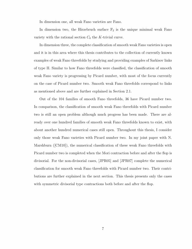
In dimension one, all weak Fano varieties are Fano.

In dimension two, the Hirzebruch surface F2 is the unique minimal weak Fano

variety with the rational section C0 the K-trivial curve.

In dimension three, the complete classification of smooth weak Fano varieties is open

and it is in this area where this thesis contributes to the collection of currently known

examples of weak Fano threefolds by studying and providing examples of Sarkisov links

of type II. Similar to how Fano threefolds were classified, the classification of smooth

weak Fano variety is progressing by Picard number, with most of the focus currently

on the case of Picard number two. Smooth weak Fano threefolds correspond to links

as mentioned above and are further explained in Section 2.1.

Out of the 104 families of smooth Fano threefolds, 36 have Picard number two.

In comparison, the classification of smooth weak Fano threefolds with Picard number

two is still an open problem although much progress has been made. There are al-

ready over one hundred families of smooth weak Fano threefolds known to exist, with

about another hundred numerical cases still open. Throughout this thesis, I consider

only those weak Fano varieties with Picard number two. In my joint paper with N.

Marshburn ([CM10]), the numerical classification of these weak Fano threefolds with

Picard number two is completed when the Mori contraction before and after the flop is

divisorial. For the non-divisorial cases, [JPR05] and [JPR07] complete the numerical

classification for smooth weak Fano threefolds with Picard number two. Their contri-

butions are further explained in the next section. This thesis presents only the cases

with symmetric divisorial type contractions both before and after the flop.

7

1.3 Prior Results and Background Information

In Germany in 2005, Priska Jahnke, Thomas Peternell, and Ivo Radloff began the clas-

sification of smooth weak Fano threefolds with Picard number two ([JPR05]). Classi-

fication in the Fano case relied on the fact that there are two contractions of extremal

rays (Mori extremal contractions). However, if X is only assumed to be weak Fano, the

second Mori contraction is substituted by the birational contraction associated with

the base point free anticanonical linear system | −mKX | for m� 0.

Jahnke, Peternell and Radloff used Mori’s classification of extremal rays in dimen-

sion three to break the classification problem into subcases:

Theorem 1.3.1. (Mori (1982)) Let X be a smooth three dimensional projective variety.

Let R be an extremal ray on X, and let φ : X → Y be the corresponding extremal

contraction. Then only the following cases are possible:

1. Type E: R is not numerically effective. Then φ : X → Y is a divisorial con-

traction of an irreducible exceptional divisor E ⊂ X onto a curve or a point. In

addition, φ is the blow-up of the subvariety φ(E) (with the reduced structure). All

the possible types of extremal rays R which can occur in this situation are listed

in the following table, where µ(R) is the length of the extremal ray R (that is, the

number min{(−KX) · C |C ∈ R is a rational curve}) and lR is a rational curve

8

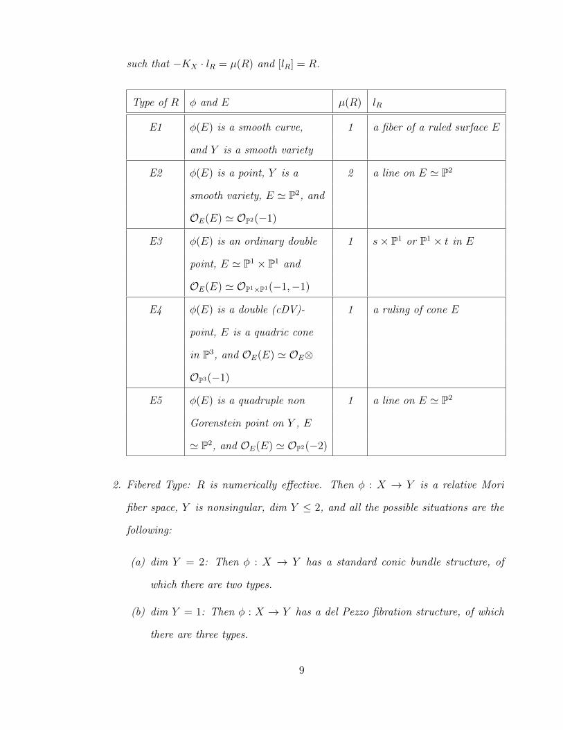
such that −KX · lR = µ(R) and [lR] = R.

Type of R φ and E µ(R) lR

E1 φ(E) is a smooth curve, 1 a fiber of a ruled surface E

and Y is a smooth variety

E2 φ(E) is a point, Y is a 2 a line on E ' P2

smooth variety, E ' P2, and

OE(E) ' OP2(−1)

E3 φ(E) is an ordinary double 1 s× P1 or P1 × t in E

point, E ' P1 × P1 and

OE(E) ' OP1×P1(−1,−1)

E4 φ(E) is a double (cDV)- 1 a ruling of cone E

point, E is a quadric cone

in P3, and OE(E) ' OE⊗

OP3(−1)

E5 φ(E) is a quadruple non 1 a line on E ' P2

Gorenstein point on Y , E

' P2, and OE(E) ' OP2(−2)

2. Fibered Type: R is numerically effective. Then φ : X → Y is a relative Mori

fiber space, Y is nonsingular, dim Y ≤ 2, and all the possible situations are the

following:

(a) dim Y = 2: Then φ : X → Y has a standard conic bundle structure, of

which there are two types.

(b) dim Y = 1: Then φ : X → Y has a del Pezzo fibration structure, of which

there are three types.

9

(c) dim Y = 0. Then X is Fano.

See [IP99] for more details regarding the fibered cases, which are not needed in this

thesis.

In [JPR05], the authors completed the numerical classification and partial geometric

classification when the anti-canonical morphism ψ|−mKX | : X → X ′ contracts a divisor.

The geometric existence of several numerical cases in their paper still remain open.

In 2007, Jahnke, Peternell, and Radloff ([JPR07]) then studied the case when the

anticanonical morphism ψ|−mKX | : X → X ′ contracts only a finite number of curves

(i.e. when ψ|−mKX | is small). They again divided their classification into subcases

based on the possible Mori contractions. Concurrently in Japan, Kiyohiko Takeuchi

also wrote a paper ([Tak09]) with a partial geometric and numerical classification of

smooth weak Fano varieties with ψ|−mKX | : X → X ′ small and one of the Mori extremal

contractions of del-Pezzo type. Due to a discrepancy in the literature between the use

of “weak Fano” and “almost Fano”, it appears that Takeuchi was unaware of the work

of Jahnke, Peternell, and Radloff and vice versa.

The authors of [JPR07] left the classification of one subcase open: when both Mori

contractions are divisorial (of type E) both before and after the flop. They stated in

their introduction that they wished to return to finish this last case; however, they

never did. This thesis, along with the thesis of N. Marshburn [Mar11], finishes the

numerical classification of this last subcase as well as achieves partial results in the

geometric realizability of some these cases. Our joint results can be found in our paper

[CM10].

10

1.4 Assumptions

Throughout this thesis, complex projective threefolds X are assumed to satisfy the

following conditions:

i) X is smooth;

ii) −KX is nef and big (i.e. X is a weak Fano variety);

iii) X has finitely many K-trivial curves (i.e. −KX is big in codimension 1);

iv) ρ(X) = 2;

v) The linear system | −KX | is basepoint free;

vi) The weak Fano index rX of X is 1.

These varieties appear as smooth central objects of Sarkisov links between termi-

nal Fano varieties with Picard number one. Classifying these links is a step toward

classifying all birational maps between terminal Fano varieties with Picard number

one.

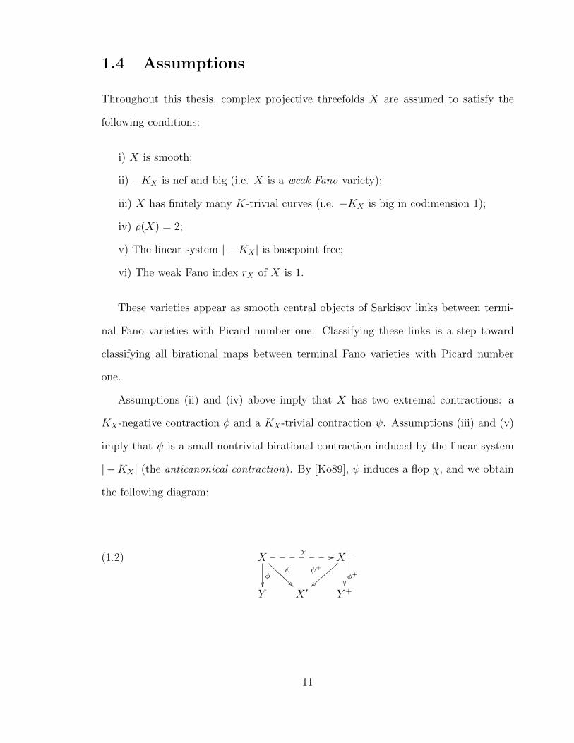
Assumptions (ii) and (iv) above imply that X has two extremal contractions: a

KX-negative contraction φ and a KX-trivial contraction ψ. Assumptions (iii) and (v)

imply that ψ is a small nontrivial birational contraction induced by the linear system

| −KX | (the anticanonical contraction). By [Ko89], ψ induces a flop χ, and we obtain

the following diagram:

(1.2) Xχ //_______

φ��

ψ

AAA

AAAA

A X+

φ+

��

ψ+

}}zzzzzzzz

Y X ′ Y +

11

In the above diagram, χ is a flop which is an isomorphism outside of the exceptional

locus Exc(ψ) and X+ satisfies the conditions (i)-(vi) above. The morphism φ+ is a

KX+-negative extremal contraction and ψ+ is the anticanonical morphism. X ′ is a

terminal Gorenstein Fano threefold with Picard number one, but is not Q-factorial

since ψ is small. Indeed, if X ′ were Q-factorial, then for a curve C contracted by ψ,

we would have 0 6= E.C = ψ∗(E).ψ∗(C) = 0. The diagram represents a Sarkisov link

of type II between the Mori fibrations Y /Spec C and Y +/Spec C.

We can further assume that −KX is generated by global sections (assumption (v)).

The case when −KX is not generated by global sections is the case when X ′ is the

deformation of the Fano threefold V2. This is proved in Proposition 2.5 in [JPR07].

If −KX is divisible in Pic(X), then −KX = rXH for some H ∈ Pic(X), where rX

is called the Fano index of X. The divisor H is called the fundamental divisor and the

linear system |H| is the fundamental system on X. The self intersection number H3 is

the degree of X. Since we are assuming X to be smooth (and in particular Gorenstein),

we remark that the Fano index rX is a positive integer. By using the smoothing of

X ′, [Shi89] has shown that rX ≤ 4, with equality when X ′ = P3. In addition, [Shi89]

showed that when rX = 3, X ′ ⊂ P4 is the quadric. In both cases, X ∼= X+. For

rX = 3, both φ and φ+ are conic P2-bundles over P1. See [JPR07] Proposition 2.12 for

more details.

The case rX = 2 was treated in [JP06]. Both φ and φ+ are either E2 contractions,

P1-bundles or quadric bundles. The complete list for the case when rX = 2, ρ(X) = 2

and ψ small is given in [JPR07] Theorem 2.13. Thus we can assume that rX = 1,

which is assumption (vi) above.

Lastly, note the result of Remark 4.1.10 in [IP99] concerning the case when X is

hyperelliptic (that is, the anticanonical map ϕ|−KX | is generically a double cover). If

the anticanonical morphism is generically a double cover of a Q-factorial threefold then

12

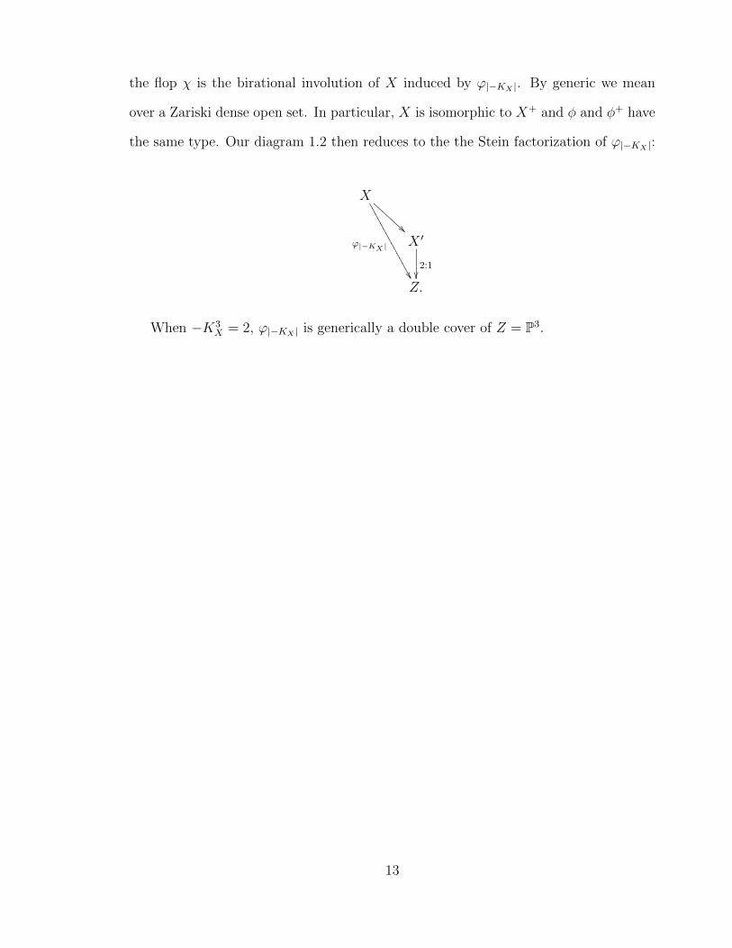
the flop χ is the birational involution of X induced by ϕ|−KX |. By generic we mean

over a Zariski dense open set. In particular, X is isomorphic to X+ and φ and φ+ have

the same type. Our diagram 1.2 then reduces to the the Stein factorization of ϕ|−KX |:

X

BBB

BBBB

ϕ|−KX |

��111111111111111

X ′

2:1��Z.

When −K3X = 2, ϕ|−KX | is generically a double cover of Z = P3.

13

Chapter 2

Relation to Mori Minimal Model

Program

As described in the introduction, the algorithm of factoring a birational map of Mori fi-

brations α : Y/S 99K Y ′/S ′ is called the Sarkisov program. In dimension two, the links

are known and the Sarkisov program leads to a new proof of the classical Castelnuovo-

Noether Theorem, which states that the group of birational self-maps of P2 is generated

by the projective linear transformations together with a fixed quadratic transforma-

tion. It is hoped that in higher dimensions the Sarkisov program can be used to

classify birational self-maps of Pn or other Mori fibrations. In this chapter we give the

definition and structure of the four types of Sarkisov links in dimension three. The

particular interest of this thesis is when both sides of the diagram (1.1) are divisorial,

corresponding to those links of type II.

14

2.1 Dimension Three Sarkisov Links

2.1.1 Definition

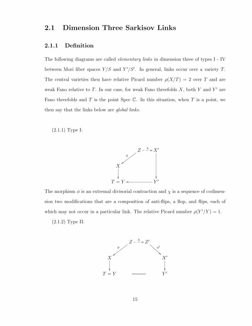
The following diagrams are called elementary links in dimension three of types I - IV

between Mori fiber spaces Y/S and Y ′/S ′. In general, links occur over a variety T .

The central varieties then have relative Picard number ρ(X/T ) = 2 over T and are

weak Fano relative to T . In our case, for weak Fano threefolds X, both Y and Y ′ are

Fano threefolds and T is the point Spec C. In this situation, when T is a point, we

then say that the links below are global links.

(2.1.1) Type I:

Zχ //___

φ

{{wwwwwwwww

X ′

��

X

��T = Y Y ′oo

The morphism φ is an extremal divisorial contraction and χ is a sequence of codimen-

sion two modifications that are a composition of anti-flips, a flop, and flips, each of

which may not occur in a particular link. The relative Picard number ρ(Y ′/Y ) = 1.

(2.1.2) Type II:

Zχ //___

φ

{{wwwwwwwww

Z ′

φ′

BBB

BBBB

B

X

��

X ′

��T = Y Y ′

15

Both φ and φ′ are divisorial contractions and χ is a sequence of codimension two

modifications that are a composition of anti-flips, a flop, and flips, each of which may

not occur in a particular link. Note that Y and Y ′ are isomorphic.

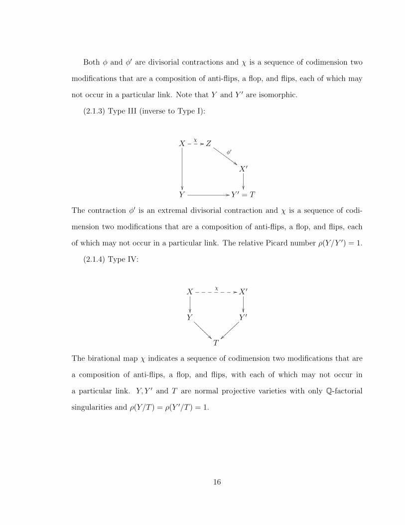
(2.1.3) Type III (inverse to Type I):

Xχ //___

��

Zφ′

##HHH

HHHH

HH

X ′

��Y // Y ′ = T

The contraction φ′ is an extremal divisorial contraction and χ is a sequence of codi-

mension two modifications that are a composition of anti-flips, a flop, and flips, each

of which may not occur in a particular link. The relative Picard number ρ(Y/Y ′) = 1.

(2.1.4) Type IV:

Xχ //_______

��

X ′

��Y

��@@@

@@@@

@ Y ′

~~}}}}}}}}

T

The birational map χ indicates a sequence of codimension two modifications that are

a composition of anti-flips, a flop, and flips, with each of which may not occur in

a particular link. Y, Y ′ and T are normal projective varieties with only Q-factorial

singularities and ρ(Y/T ) = ρ(Y ′/T ) = 1.

16

Chapter 3

E1-E1 Case

3.1 Equations and Bounds

Let us consider first the case where both extremal contractions φ and φ+ are of type

E1. Then Y is a smooth Fano variety of Fano index r with Picard number one, and φ

is the blow up of a smooth curve C ⊂ Y . Let g and d denote the genus and degree of C

and let E denote the exceptional divisor φ−1(C). Denote by H a fundamental divisor

in Y . The pullback of H to X will also be denoted by H. Since Pic(Y ) is generated

by H, Pic(X) ∼= Z ⊕ Z is generated by H and E. We will use the divisors −KX and

E as generators of Pic(X) instead. Unless the Fano index of Y is one, these divisors

do not generate Pic(X). However, they do generate Pic(X) ⊗ Q, the Picard group of

X with coefficients in Q.

The strict transform of a divisor D ∈ Pic(X) across the flop χ is denoted by D.

Since χ is small, KX = KX+ . We identify divisors in X and X+ via χ and thus

have an isomorphism between the Picard groups of X and X+. In particular, for any

D ∈ Pic(X), χ−1(χ(D)) = D and for any D+ ∈ Pic(X+), χ(χ−1(D+)) = D+. In our

notation, we can write this as˜D = D.

17

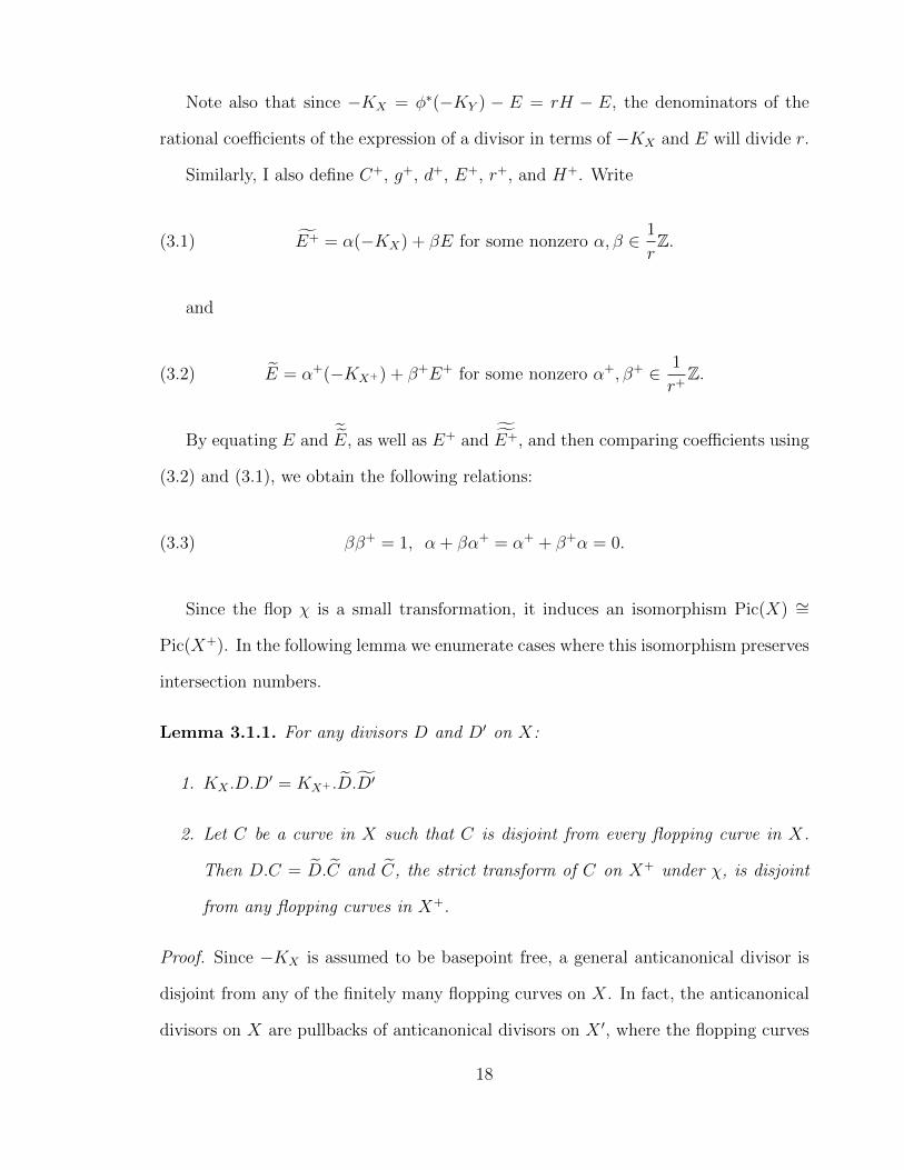
Note also that since −KX = φ∗(−KY ) − E = rH − E, the denominators of the

rational coefficients of the expression of a divisor in terms of −KX and E will divide r.

Similarly, I also define C+, g+, d+, E+, r+, and H+. Write

(3.1) E+ = α(−KX) + βE for some nonzero α, β ∈ 1

rZ.

and

(3.2) E = α+(−KX+) + β+E+ for some nonzero α+, β+ ∈ 1

r+Z.

By equating E and˜E, as well as E+ and

˜E+, and then comparing coefficients using

(3.2) and (3.1), we obtain the following relations:

(3.3) ββ+ = 1, α + βα+ = α+ + β+α = 0.

Since the flop χ is a small transformation, it induces an isomorphism Pic(X) ∼=

Pic(X+). In the following lemma we enumerate cases where this isomorphism preserves

intersection numbers.

Lemma 3.1.1. For any divisors D and D′ on X:

1. KX .D.D′ = KX+ .D.D′

2. Let C be a curve in X such that C is disjoint from every flopping curve in X.

Then D.C = D.C and C, the strict transform of C on X+ under χ, is disjoint

from any flopping curves in X+.

Proof. Since −KX is assumed to be basepoint free, a general anticanonical divisor is

disjoint from any of the finitely many flopping curves on X. In fact, the anticanonical

divisors on X are pullbacks of anticanonical divisors on X ′, where the flopping curves

18

are contracted to finitely many points. The theorem then follows from the projection

formula.

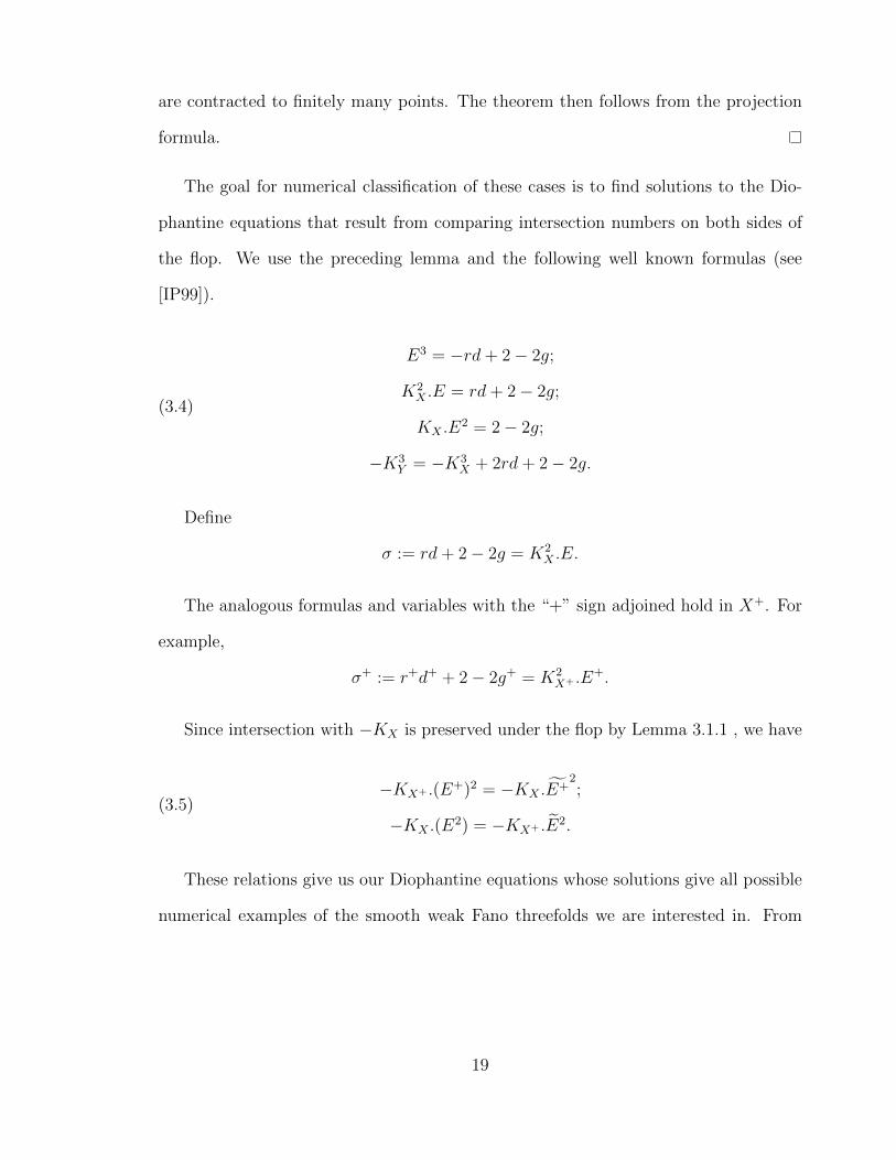
The goal for numerical classification of these cases is to find solutions to the Dio-

phantine equations that result from comparing intersection numbers on both sides of

the flop. We use the preceding lemma and the following well known formulas (see

[IP99]).

(3.4)

E3 = −rd+ 2− 2g;

K2X .E = rd+ 2− 2g;

KX .E2 = 2− 2g;

−K3Y = −K3

X + 2rd+ 2− 2g.

Define

σ := rd+ 2− 2g = K2X .E.

The analogous formulas and variables with the “+” sign adjoined hold in X+. For

example,

σ+ := r+d+ + 2− 2g+ = K2X+ .E+.

Since intersection with −KX is preserved under the flop by Lemma 3.1.1 , we have

(3.5)−KX+ .(E+)2 = −KX .E+

2;

−KX .(E2) = −KX+ .E2.

These relations give us our Diophantine equations whose solutions give all possible

numerical examples of the smooth weak Fano threefolds we are interested in. From

19

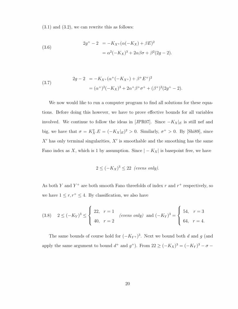
(3.1) and (3.2), we can rewrite this as follows:

(3.6)2g+ − 2 = −KX+(α(−KX) + βE)2

= α2(−KX)3 + 2αβσ + β2(2g − 2).

(3.7)2g − 2 = −KX+(α+(−KX+) + β+E+)2

= (α+)2(−KX)3 + 2α+β+σ+ + (β+)2(2g+ − 2).

We now would like to run a computer program to find all solutions for these equa-

tions. Before doing this however, we have to prove effective bounds for all variables

involved. We continue to follow the ideas in [JPR07]. Since −KX |E is still nef and

big, we have that σ = K2X .E = (−KX |E)2 > 0. Similarly, σ+ > 0. By [Shi89], since

X ′ has only terminal singularities, X ′ is smoothable and the smoothing has the same

Fano index as X, which is 1 by assumption. Since | −KX | is basepoint free, we have

2 ≤ (−KX)3 ≤ 22 (evens only).

As both Y and Y + are both smooth Fano threefolds of index r and r+ respectively, so

we have 1 ≤ r, r+ ≤ 4. By classification, we also have

(3.8) 2 ≤ (−KY )3 ≤

22, r = 1

40, r = 2(evens only) and (−KY )3 =

54, r = 3

64, r = 4.

The same bounds of course hold for (−KY +)3. Next we bound both d and g (and

apply the same argument to bound d+ and g+). From 22 ≥ (−KX)3 = (−KY )3 − σ −

20

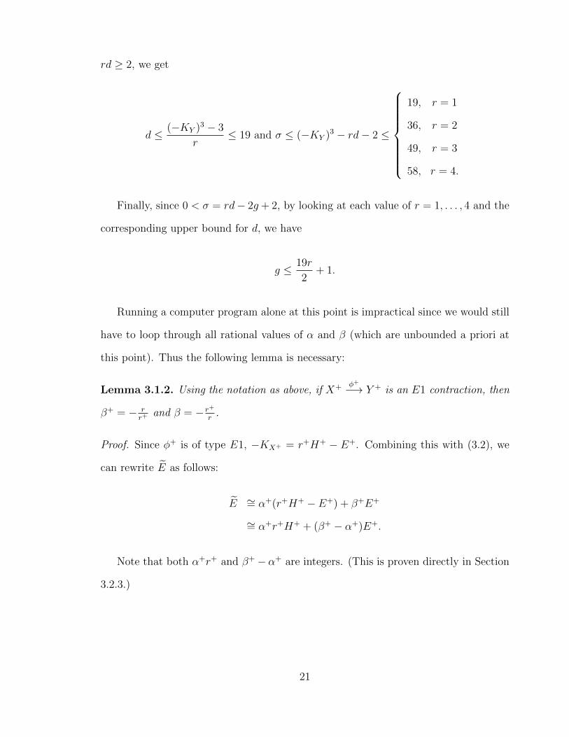
rd ≥ 2, we get

d ≤ (−KY )3 − 3

r≤ 19 and σ ≤ (−KY )3 − rd− 2 ≤

19, r = 1

36, r = 2

49, r = 3

58, r = 4.

Finally, since 0 < σ = rd− 2g + 2, by looking at each value of r = 1, . . . , 4 and the

corresponding upper bound for d, we have

g ≤ 19r

2+ 1.

Running a computer program alone at this point is impractical since we would still

have to loop through all rational values of α and β (which are unbounded a priori at

this point). Thus the following lemma is necessary:

Lemma 3.1.2. Using the notation as above, if X+ φ+−→ Y + is an E1 contraction, then

β+ = − rr+

and β = − r+

r.

Proof. Since φ+ is of type E1, −KX+ = r+H+ − E+. Combining this with (3.2), we

can rewrite E as follows:

E ∼= α+(r+H+ − E+) + β+E+

∼= α+r+H+ + (β+ − α+)E+.

Note that both α+r+ and β+ − α+ are integers. (This is proven directly in Section

3.2.3.)

21

Thus

Z/rZ ∼= Pic(X)/〈−KX , E〉

∼= Pic(X+)/〈−KX+ , E〉

∼= Pic(X+)/〈r+H+ − E+, α+r+H+ + (β+ − α+)E+〉.

Taking the order of both sides yields:

r =

∣∣∣∣∣∣∣α+r+ r+

β+ − α+ −1

∣∣∣∣∣∣∣ = −α+r+ − r+β+ + α+r+ = −r+β+

and thus β+ = − rr+

as desired.

From (3.3), it then follows that β = − r+

r.

Notice now that both α+, and then by (3.3) α, are completely determined by

replacing (3.2) into the formula for σ:

σ = K2X .E = K2

X+E = α+(−KX+)3 + β+K2X+E+.

Thus

(3.9) α+ =σ − β+σ+

(−KX)3.

We include the following two formulas for completeness:

(3.10) E3 = (α+)3(−KX)3 + 3(α+)2β+σ+ − 3α+(β+)2KX(E+)2 + (β+)3(E+)3;

(3.11) E+3

= α3(−KX)3 + 3α2βσ − 3αβ2KXE2 + β3E3.

22

All our variables are now bounded or completely determined via an explicit formula.

With our equations finalized, we are ready to run a computer program to find all the

possible numerical solutions. Programs were written in both Visual Basic and C++ to

verify the results. The Visual Basic source code can be found in the Appendix 5.4 of

this thesis. Here we summarize our bounds on the variables used in the program.

Variables and bounds:

1 ≤ r, r+ ≤ 4;

2 ≤ K3X ≤ 22 (evens only);

0 ≤ g ≤ 19r

+ 1;

0 ≤ g+ ≤ 19r+

+ 1;

1 ≤ d, d+ ≤ 19.

From these variables, the following are then determined:

−K3Y = −K3

X + 2rd− 2g + 2;

−K3Y + = −K3

X + 2r+d+ − 2g+ + 2;

σ = rd+ 2− 2g;

σ+ = r+d+ + 2− 2g+;

β+ = − rr+

;

β = 1β+ ;

α+ = σ−β+σ+

−K3X

;

α = −βα+.

Equations that any weak Fano threefold with our assumptions must satisfy (3.5):

2g+ − 2 = α2(−KX)3 + 2αβσ + β2(2g − 2);

2g − 2 = (α+)2(−KX)3 + 2α+β+σ+ + (β+)2(2g+ − 2).

The programs used to create tables (5.1),(5.2),(5.3), and (5.4) of this thesis are available

23

to view in Appendix (5.4) as well as download from the author’s website:

www.math.jhu.edu\ ∼ jcutrone.

3.2 Numerical Checks

Although a computer program can now be run from the results of the prior section,

there are still numerical checks that can be added to the program to eliminate some

possible solutions. Some simple numerical checks to include in the program have been

previously mentioned, such as (3.3) and checking that both σ, σ+ > 0. From the

classification of smooth Fano threefolds Y with Picard number one, we also have to

check that both (−KY )3 and (−KY +)3 are even and that both these numbers satisfy

the bounds from (3.8). In addition, again from classification, we have to check that if

r = 1, (−KY )3 6= 20 and similarly if r+ = 1, (−KY +)3 6= 20.

Another obvious check to include in the program is that r3 divides (−KY )3 and

that (r+)3 divides (−KY +)3. Using the formulas in (3.10) and (3.11), we also need to

make sure both E3 and E+3∈ Z.

Define the defect of the flop to be

(3.12) e = E3 − E3.

Then we have the following two lemmas, which add two more checks to our growing

list.

Lemma 3.2.1. [Tak02] The correction term e in (3.12) is a strictly positive integer

24

For a simpler proof then that of [Tak02] in the above Lemma, see the proof of

Lemma 3.1 in [Kal09].

The integer e is not widely understood. It is related to the number of flopping

curves, and in fact is equal to this number if the flop is an Atiyah flop and if for each

flopping curve Γ we have H.Γ = 1. See [Mar11] for more details regarding the integer

e when the flop is a simple Atiyah flop. At present, there is no known upper bound. In

my tables, I still have open examples with very large values of e. If a strict upper bound

could be found, then this bound could be used to eliminate the geometric realization

of some open cases.

Lemma 3.2.2. The integer r3 divides e.

Proof. Starting from the equality E = rH+KX , take the strict transform of E under χ

to get E = ( ˜rH +KX) = rH +KX+ . Taking the difference of cubes in the formula for

e and using the facts that −K3X = −K3

X+ and that intersection with KX is preserved

under a flop (Lemma 3.1.1) we get the desired result.

Since E+ = α(−KX)+βE, by replacing −KY with rH and −KX with −KY −E =

rH − E, we have

(3.13) E+ = αrH + (β − α)E.

Since E+ ∈ Pic(X) is not divisible, we have the following:

Proposition 3.2.3. Using all notation as above, we have the following numerical

checks:

αr, α+r+, α− β, α+ − β+ ∈ Z;

GCD(αr, β − α) = 1;

GCD(α+r+, β+ − α+) = 1.

25

Since we are assuming X is smooth, we can use the results of Batyrev and Kont-

sevich (see [Ba97]) which state that Hodge numbers are preserved under a flop. The

only interesting Hodge number in our situation is h1,2(X). For smooth Fano threefolds

Y with Picard number one, all these numbers are known (see [IP99]). In the E1 case,

since we are blowing up a smooth curve of genus g, it can be shown (see [CG72]) that

h1,2(X) = h1,2(Y ) + g. Thus checking to see if h1,2(X) = h1,2(X+) is equivalent to

checking the following equality:

(3.14) h1,2(Y ) + g = h1,2(Y +) + g+.

Using these checks to eliminate some possible cases from the output of the computer

program yields Table (5.1) in the Tables section of this thesis.

Theorem 3.2.4. For a geometrically realizable link (1.2), if both φ and φ+ are of

type E1, then the numerical invariants associate to the link are found in Table (5.1).

Thirteen families of these links exist are known to exist.

3.3 Elimination of Cases

In this section, we will eliminate some of the numerical cases listed in Table (5.1).

Proposition 3.3.1. The following E1-E1 numerical cases in Table (5.1) are not geo-

metrically realizable:

Nos. 27, 32, 36, 53, 62, 66, 73, 82, 85, 91, 95.

Proof. We will show that case No. 27 can not exist. A similar argument can be applied

26

to the remaining cases. From the data in case No. 27, we have that

E+ ∼ −4KX − E

∼ 4(−KY − E)− E

∼ 4(2H − E)− E

∼ 8H − 5E.

Since E+ is the strict transform of an exceptional divisor, E+ must be the unique

member of the linear system |E+|. However, since

|E+| = |8H − 5E| ⊃ 5|H − E|+ 3|H|

and since dim |H| > 0, the linear system |H − E| must be empty. We will show that

this is in fact not the case.

To show that |H − E| 6= ∅, it is equivalent to show that h0(X,H − E) > 0. Since

we are in the E1 case, this is in turn equivalent to showing that h0(Y,H − C) > 0,

where C is the smooth curve of genus 0 and degree 1 being blown up. The inequality

h0(Y,H −C) > 0 is equivalent to h0(Y, IC(H)) > 0, which is what we will show. Here

IC is the ideal sheaf of the curve C on Y .

Start with the short exact sequence:

0→ IC → OY → OC → 0.

Twist by H to get the short exact sequence:

0→ IC(H)→ OY (H)→ OC(H)→ 0.

27

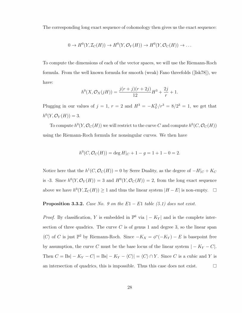
The corresponding long exact sequence of cohomology then gives us the exact sequence:

0→ H0(Y, IC(H))→ H0(Y,OY (H))→ H0(Y,OC(H))→ . . .

To compute the dimensions of each of the vector spaces, we will use the Riemann-Roch

formula. From the well known formula for smooth (weak) Fano threefolds ([Isk78]), we

have:

h0(X,OX(jH)) =j(r + j)(r + 2j)

12H3 +

2j

r+ 1.

Plugging in our values of j = 1, r = 2 and H3 = −K3Y /r

3 = 8/23 = 1, we get that

h0(Y,OY (H)) = 3.

To compute h0(Y,OC(H)) we will restrict to the curve C and compute h0(C,OC(H))

using the Riemann-Roch formula for nonsingular curves. We then have

h0(C,OC(H)) = degH|C + 1− g = 1 + 1− 0 = 2.

Notice here that the h1(C,OC(H)) = 0 by Serre Duality, as the degree of −H|C +KC

is -3. Since h0(Y,OY (H)) = 3 and H0(Y,OC(H)) = 2, from the long exact sequence

above we have h0(Y, IC(H)) ≥ 1 and thus the linear system |H −E| is non-empty.

Proposition 3.3.2. Case No. 9 on the E1− E1 table (5.1) does not exist.

Proof. By classification, Y is embedded in P6 via | − KY | and is the complete inter-

section of three quadrics. The curve C is of genus 1 and degree 3, so the linear span

〈C〉 of C is just P2 by Riemann-Roch. Since −KX = φ∗(−KY ) − E is basepoint free

by assumption, the curve C must be the base locus of the linear system | −KY − C|.

Then C = Bs| −KY − C| = Bs| −KY − 〈C〉| = 〈C〉 ∩ Y . Since C is a cubic and Y is

an intersection of quadrics, this is impossible. Thus this case does not exist.

28

3.4 Geometric Realization of Cases

In this section we discuss the geometric realization of some of the cases found in Table

5.1.

Remark 3.4.1. Some of the cases listed in Table 5.1 were previously shown to exist as

weak Fano varieties by Takeuchi. In other instances, the methods used by Iskovskikh

and others to show the existence of the smooth Fano threefold with the same numerical

invariants directly apply. These cases are mentioned with their appropriate references

in the corresponding tables.

Proposition 3.4.2. Case No. 111 on the E1− E1 table (5.1) exists.

Proof. Let S ⊂ P3 be a nonsingular cubic surface, the blow-up of P2 at six general

points (no three on a line, no six on a conic). Let the Picard group of S be generated

by l, e1, . . . , e6, where l is the pullback of a line in P2 and e1, . . . , e6 are the exceptional

divisors. The intersection numbers between the generators of Pic(S) are l2 = 1, l.ei = 0

for any i = 1, . . . , 6 and ei.ej = −δij, where δij is the Kronecker delta. In S, consider

the divisor

C ∼ 7l − 4e1 − 3e2 − 3e3 − 2e4 − 2e5 − 2e6.

Since for any of the 27 lines L on S, C.L ≥ 0 and C2 > 0, by the theory of cubic

surfaces ([Ha77]), the linear system |C| contains an irreducible nonsingular member

which we will also denote by C.

The degree of any effective divisor D ∼ al −∑biei on S as a curve in P3 is

3a−∑bi, and the genus of D is 1

2(a− 1)(a− 2)− 1

2

∑(b2i − bi). Thus the degree and

genus of C are 5 and 0 respectively, in accordance with the given data. Let X be the

blowup of C in P3. Let S in X be the strict transform of the cubic surface S. Then

S ∈ |3H − E| = | −KX −H|.

29

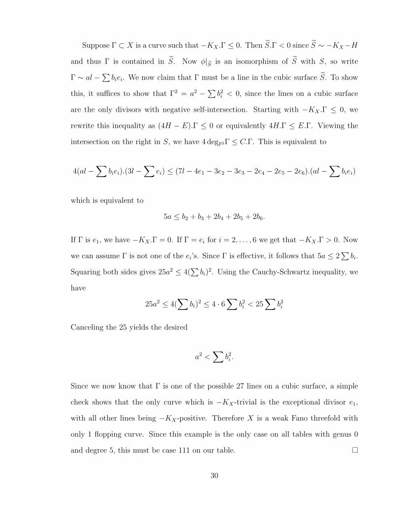
Suppose Γ ⊂ X is a curve such that −KX .Γ ≤ 0. Then S.Γ < 0 since S ∼ −KX−H

and thus Γ is contained in S. Now φ|S is an isomorphism of S with S, so write

Γ ∼ al −∑biei. We now claim that Γ must be a line in the cubic surface S. To show

this, it suffices to show that Γ2 = a2 −∑b2i < 0, since the lines on a cubic surface

are the only divisors with negative self-intersection. Starting with −KX .Γ ≤ 0, we

rewrite this inequality as (4H − E).Γ ≤ 0 or equivalently 4H.Γ ≤ E.Γ. Viewing the

intersection on the right in S, we have 4 degP3Γ ≤ C.Γ. This is equivalent to

4(al −∑

biei).(3l −∑

ei) ≤ (7l − 4e1 − 3e2 − 3e3 − 2e4 − 2e5 − 2e6).(al −∑

biei)

which is equivalent to

5a ≤ b2 + b3 + 2b4 + 2b5 + 2b6.

If Γ is e1, we have −KX .Γ = 0. If Γ = ei for i = 2, . . . , 6 we get that −KX .Γ > 0. Now

we can assume Γ is not one of the ei’s. Since Γ is effective, it follows that 5a ≤ 2∑bi.

Squaring both sides gives 25a2 ≤ 4(∑bi)

2. Using the Cauchy-Schwartz inequality, we

have

25a2 ≤ 4(∑

bi)2 ≤ 4 · 6

∑b2i < 25

∑b2i

Canceling the 25 yields the desired

a2 <∑

b2i .

Since we now know that Γ is one of the possible 27 lines on a cubic surface, a simple

check shows that the only curve which is −KX-trivial is the exceptional divisor e1,

with all other lines being −KX-positive. Therefore X is a weak Fano threefold with

only 1 flopping curve. Since this example is the only case on all tables with genus 0

and degree 5, this must be case 111 on our table.

30

Remark 3.4.3. Case No. 76: This case is shown to exist in [JPR05], page 40, in their

example No. 19.

31

Chapter 4

Non E1-E1 Cases

4.1 Numerical Classification

In this section we assume both φ : X → Y and φ+ : X+ → Y + are both either

E2, E3/E4 or E5 contractions. The cases E3 and E4 are numerically equivalent, and

thus we do not distinguish between them in what follows. We start the classification

of these remaining divisorial type contractions with the following observation:

Proposition 4.1.1. If φ : X → Y is an E2, E3/E4 or E5 type contraction, then α

and β as in (3.1) are integers.

Proof. Case 1: The contraction φ is E2 : If the Fano index of Y , rY , is two, then

the Fano index of X, would be two, contradicting our assumption that rX = 1. By

classification of smooth Fano threefolds with Picard number one, if rY = 3 or 4, then

Y is either the smooth quadric Q ⊂ P4 or P3 respectively. In both of these situations,

the blow up of a point would be a Fano variety. Thus we only need to consider the

case when Y has Fano index one. Let l be a line on Y which we know to exist by the

classic theorem of Shokurov.

Then −KX .φ∗(l) = −KY .l = 1 and E.φ∗(l) = 0. Therefore Z 3 E+.φ∗(l) =

32

(α(−KX) + βE).φ∗(l) = α. Therefore E+ + αKX = βE is Cartier, so β ∈ Z.

Case 2: φ is E3/E4 or E5 : Let ψ be the flopping contraction. Then ψ restricted to

E is a finite birational morphism. The linear system corresponding to the morphism

ψ|E is the subsystem of | − KX |E| corresponding to the image of H0(X,−KX) →

H0(X,−KX |E). By Mori’s theorem classifying extremal rays (1.3.1), we know that

in the E3/E4 case, OX(−KX)|E ∼= OQ(1) on a quadric Q ⊂ P3 and for the E5

case, OX(−KX)|E ∼= OP2(1) on P2. No proper subsystem of either of the com-

plete linear systems associated to these sheaves gives a finite birational morphism,

so H0(X,−KX)→ H0(X,−KX |E) is surjective. Therefore the linear system of ψ|E is

|−KX |E|. Thus ψ|E is an embedding since −KX |E = O(1) is very ample. This implies

the intersection of E with any flopping curve Γ must be transversal at a single point,

ie E.Γ = 1. Then Z 3 E+.Γ = (α(−KX) + βE).Γ = β. So E+ − βE = α(−KX) is

Cartier and since the index of X is 1 by assumption, α ∈ Z.

By the above proposition, we immediately obtain:

Lemma 4.1.2. If Xφ−→ Y and X+ φ+−→ Y + are both contractions of type either

E2, E3/E4 or E5, then α = α+ and β = β+ = −1.

Proof. Since β and β+ are both negative integers and ββ+ = 1 by (3.3), we must have

β = β+ = −1. Since α + βα+ = 0, we get α = α+.

We now proceed to show which combinations of symmetric E2 − E5 contractions

can exist. Note first that by Theorem 1.3.1, a simple calculation shows that KX .E2 = 2

33

for any contraction of type E2, E3/E4, or E5. Then

2 = KX+ .E+2

= KX .E+2

= KX .(−αKX − E)2

= α2K3X + 2αK2

X .E +KX .E2

= α(αK3X + 2K2

X .E) + 2.

Since α 6= 0 by (3.1), we obtain:

−K3X =

2K2X .E

α.

By symmetry, this formula also holds for φ+. That is,

−K3X+ =

2K2X+ .E+

α+.

Recalling that −K3X = −K3

X+ and α = α+, we have K2X .E = K2

X+ .E+. Also,

K2X .E = 4, 2 or 1 for contractions of type E2, E3/E4 and E5 respectively. Using

Theorem 1.3.1, this proves the following:

Theorem 4.1.3. If Xφ→ Y is of type E2 − E5, then X+ φ+→ Y + is of the same type.

The possible values of (−K3X , α) are found in Tables 5.2, 5.3, and 5.4.

To calculate the remaining the numbers on our tables (5.2),(5.3),(5.4), we note the

following formulas for −K3Y , again using Theorem 1.3.1:

−K3Y = −K3

X + 8, φ : X → Y an E2 contraction;

−K3Y = −K3

X + 2, φ : X → Y an E3/E4 contraction;

−K3Y = −K3

X + 12, φ : X → Y an E5 contraction.

34

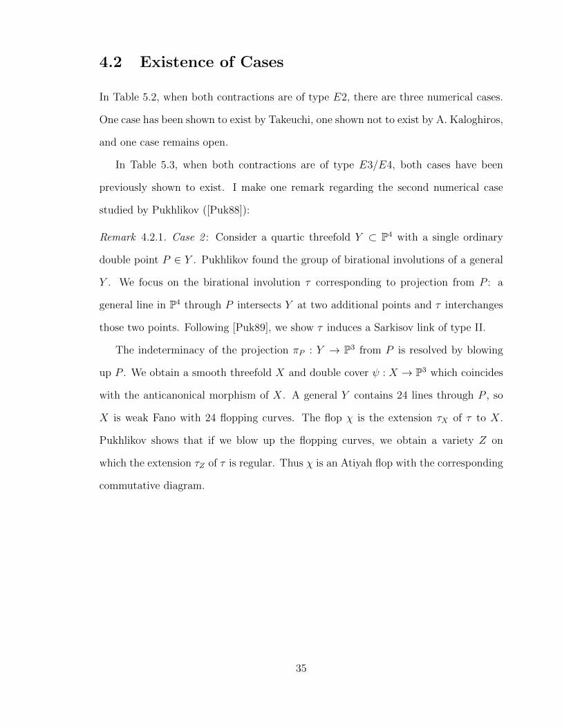
4.2 Existence of Cases

In Table 5.2, when both contractions are of type E2, there are three numerical cases.

One case has been shown to exist by Takeuchi, one shown not to exist by A. Kaloghiros,

and one case remains open.

In Table 5.3, when both contractions are of type E3/E4, both cases have been

previously shown to exist. I make one remark regarding the second numerical case

studied by Pukhlikov ([Puk88]):

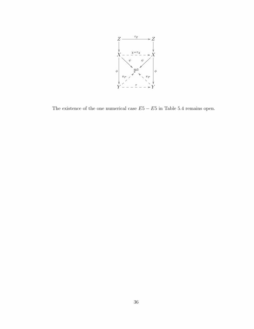
Remark 4.2.1. Case 2 : Consider a quartic threefold Y ⊂ P4 with a single ordinary

double point P ∈ Y . Pukhlikov found the group of birational involutions of a general

Y . We focus on the birational involution τ corresponding to projection from P : a

general line in P4 through P intersects Y at two additional points and τ interchanges

those two points. Following [Puk89], we show τ induces a Sarkisov link of type II.

The indeterminacy of the projection πP : Y → P3 from P is resolved by blowing

up P . We obtain a smooth threefold X and double cover ψ : X → P3 which coincides

with the anticanonical morphism of X. A general Y contains 24 lines through P , so

X is weak Fano with 24 flopping curves. The flop χ is the extension τX of τ to X.

Pukhlikov shows that if we blow up the flopping curves, we obtain a variety Z on

which the extension τZ of τ is regular. Thus χ is an Atiyah flop with the corresponding

commutative diagram.

35

Z

��

τZ // Z

��X

χ=τX //_______

φ

��

ψ

AAA

AAAA

A X

φ

��

ψ

~~}}}}}}}}

P3

Y

πP

>>}}

}}

τ //_______ Y

πP

``AAAA

The existence of the one numerical case E5− E5 in Table 5.4 remains open.

36

Chapter 5

Tables

5.1 E1 - E1

The following table is a list of all the numerical possibilities for the E1−E1 case, where

r and r+ are the Fano indices of Y and Y + in (1.2) respectively. All other notations

can be found in (3.1) and (3.2). Due to space constraints, missing from the table are

the values of α+ and β+. Those can be determined from the given values of α and β

using (3.3). There are 111 entries on the table, with 12 known not to exist, 13 known

to exist, and the remaining 86 unknown. These cases are denoted by the standard

scientific notations “x”, “ :) ”, and “?” respectively.

37

Table 5.1: E1-E1

No. −K3X −K3

Y −K3Y + α β r d g r+ d+ g+ e/r3 Exist? Ref

1. 2 6 6 3 -1 1 1 0 1 1 0 47 :) [Isk78]2. 2 8 8 4 -1 1 2 0 1 2 0 88 ?3. 2 10 10 5 -1 1 3 0 1 3 0 153 ?4. 2 12 12 6 -1 1 4 0 1 4 0 248 ?5. 2 14 14 7 -1 1 5 0 1 5 0 379 ?6. 2 16 16 8 -1 1 6 0 1 6 0 552 ?7. 2 18 18 9 -1 1 7 0 1 7 0 773 ?8. 2 22 22 11 -1 1 9 0 1 9 0 1383 ?9. 2 8 8 3 -1 1 3 1 1 3 1 21 x (3.3.2)10. 2 10 10 4 -1 1 4 1 1 4 1 56 ?11. 2 12 12 5 -1 1 5 1 1 5 1 115 ?12. 2 14 14 6 -1 1 6 1 1 6 1 204 ?13. 2 16 16 7 -1 1 7 1 1 7 1 329 ?14. 2 18 18 8 -1 1 8 1 1 8 1 496 ?15. 2 22 22 10 -1 1 10 1 1 10 1 980 ?16. 2 12 12 4 -1 1 6 2 1 6 2 24 ?17. 2 14 14 5 -1 1 7 2 1 7 2 77 ?18. 2 16 16 6 -1 1 8 2 1 8 2 160 ?19. 2 18 18 7 -1 1 9 2 1 9 2 279 ?20. 2 22 22 9 -1 1 11 2 1 11 2 649 ?21. 2 16 16 5 -1 1 9 3 1 9 3 39 ?22. 2 18 18 6 -1 1 10 3 1 10 3 116 ?23. 2 22 22 8 -1 1 12 3 1 12 3 384 ?24. 2 18 18 5 -1 1 11 4 1 11 4 1 ?25. 2 22 22 7 -1 1 13 4 1 13 4 179 ?26. 2 22 22 6 -1 1 14 5 1 14 5 28 ?27. 2 8 8 4 -1 2 1 0 2 1 0 11 x (3.3.1)28. 2 16 16 8 -1 2 3 0 2 3 0 69 ?29. 2 24 24 12 -1 2 5 0 2 5 0 223 ?30. 2 32 32 16 -1 2 7 0 2 7 0 521 ?31. 2 40 40 20 -1 2 9 0 2 9 0 1011 ?32. 2 16 16 6 -1 2 4 2 2 4 2 20 x (3.3.1)33. 2 24 24 10 -1 2 6 2 2 6 2 114 ?34. 2 32 32 14 -1 2 8 2 2 8 2 328 ?35. 2 40 40 18 -1 2 10 2 2 10 2 710 ?36. 2 24 24 8 -1 2 7 4 2 7 4 41 x (3.3.1)

37. 2 32 32 12 -1 2 9 4 2 9 4 183 ?

38

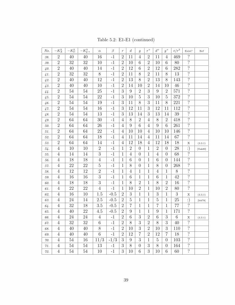
Table 5.2: E1-E1 (continued)

No. −K3X −K3


38. 2 40 40 16 -1 2 11 4 2 11 4 469 ?39. 2 32 32 10 -1 2 10 6 2 10 6 80 ?40. 2 40 40 14 -1 2 12 6 2 12 6 282 ?41. 2 32 32 8 -1 2 11 8 2 11 8 13 ?42. 2 40 40 12 -1 2 13 8 2 13 8 143 ?43. 2 40 40 10 -1 2 14 10 2 14 10 46 ?44. 2 54 54 25 -1 3 9 2 3 9 2 571 ?45. 2 54 54 22 -1 3 10 5 3 10 5 372 ?46. 2 54 54 19 -1 3 11 8 3 11 8 221 ?47. 2 54 54 16 -1 3 12 11 3 12 11 112 ?48. 2 54 54 13 -1 3 13 14 3 13 14 39 ?49. 2 64 64 30 -1 4 8 2 4 8 2 418 ?50. 2 64 64 26 -1 4 9 6 4 9 6 261 ?51. 2 64 64 22 -1 4 10 10 4 10 10 146 ?52. 2 64 64 18 -1 4 11 14 4 11 14 67 ?53. 2 64 64 14 -1 4 12 18 4 12 18 18 x (3.3.1)

54. 4 10 10 2 -1 1 2 0 1 2 0 28 :) [Tak89]

55. 4 14 14 3 -1 1 4 0 1 4 0 68 ?56. 4 18 18 4 -1 1 6 0 1 6 0 144 ?57. 4 22 22 5 -1 1 8 0 1 8 0 268 ?58. 4 12 12 2 -1 1 4 1 1 4 1 8 ?59. 4 16 16 3 -1 1 6 1 1 6 1 42 ?60. 4 18 18 3 -1 1 8 2 1 8 2 16 ?61. 4 22 22 4 -1 1 10 2 1 10 2 80 ?62. 4 16 10 1.5 -0.5 2 3 1 1 3 1 3 x (3.3.1)

63. 4 24 14 2.5 -0.5 2 5 1 1 5 1 25 :) [Isk78]

64. 4 32 18 3.5 -0.5 2 7 1 1 7 1 77 ?65. 4 40 22 4.5 -0.5 2 9 1 1 9 1 171 ?66. 4 24 24 4 -1 2 6 3 2 6 3 6 x (3.3.1)

67. 4 32 32 6 -1 2 8 3 2 8 3 40 ?68. 4 40 40 8 -1 2 10 3 2 10 3 110 ?69. 4 40 40 6 -1 2 12 7 2 12 7 18 ?70. 4 54 16 11/3 -1/3 3 9 3 1 5 0 103 ?71. 4 54 54 13 -1 3 8 0 3 8 0 164 ?72. 4 54 54 10 -1 3 10 6 3 10 6 60 ?

39

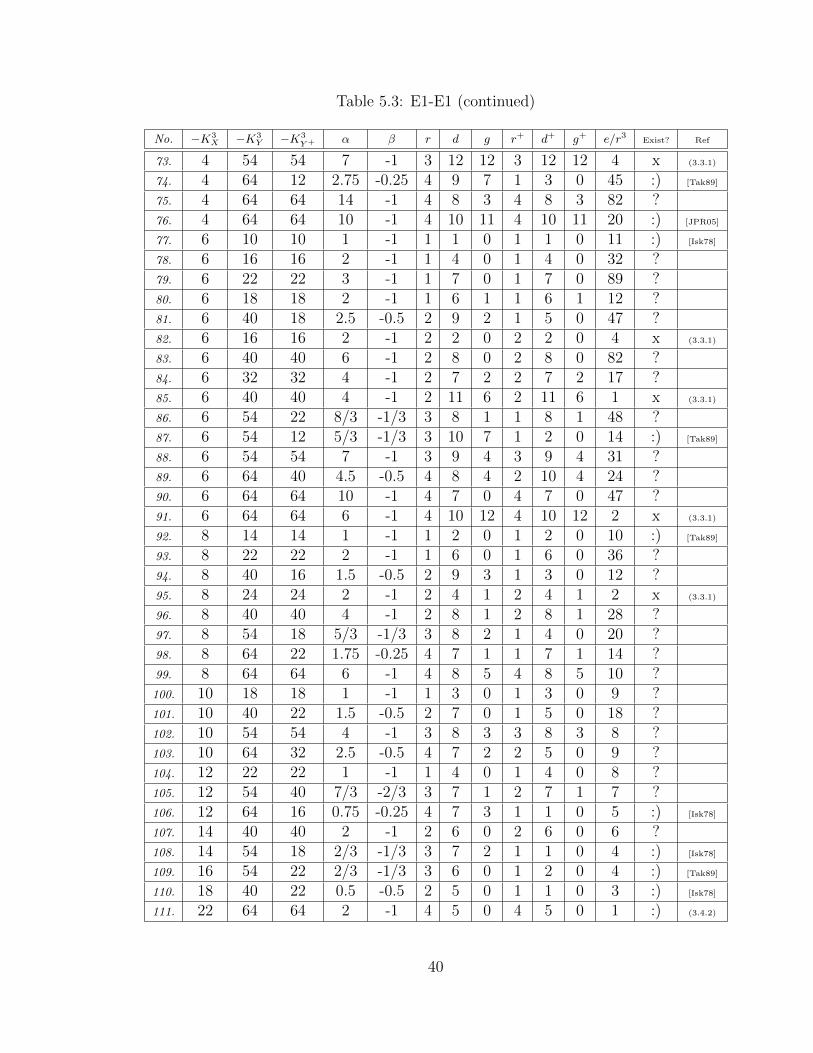
Table 5.3: E1-E1 (continued)

No. −K3X −K3


73. 4 54 54 7 -1 3 12 12 3 12 12 4 x (3.3.1)

74. 4 64 12 2.75 -0.25 4 9 7 1 3 0 45 :) [Tak89]

75. 4 64 64 14 -1 4 8 3 4 8 3 82 ?76. 4 64 64 10 -1 4 10 11 4 10 11 20 :) [JPR05]

77. 6 10 10 1 -1 1 1 0 1 1 0 11 :) [Isk78]

78. 6 16 16 2 -1 1 4 0 1 4 0 32 ?79. 6 22 22 3 -1 1 7 0 1 7 0 89 ?80. 6 18 18 2 -1 1 6 1 1 6 1 12 ?81. 6 40 18 2.5 -0.5 2 9 2 1 5 0 47 ?82. 6 16 16 2 -1 2 2 0 2 2 0 4 x (3.3.1)

83. 6 40 40 6 -1 2 8 0 2 8 0 82 ?84. 6 32 32 4 -1 2 7 2 2 7 2 17 ?85. 6 40 40 4 -1 2 11 6 2 11 6 1 x (3.3.1)

86. 6 54 22 8/3 -1/3 3 8 1 1 8 1 48 ?87. 6 54 12 5/3 -1/3 3 10 7 1 2 0 14 :) [Tak89]

88. 6 54 54 7 -1 3 9 4 3 9 4 31 ?89. 6 64 40 4.5 -0.5 4 8 4 2 10 4 24 ?90. 6 64 64 10 -1 4 7 0 4 7 0 47 ?91. 6 64 64 6 -1 4 10 12 4 10 12 2 x (3.3.1)

92. 8 14 14 1 -1 1 2 0 1 2 0 10 :) [Tak89]

93. 8 22 22 2 -1 1 6 0 1 6 0 36 ?94. 8 40 16 1.5 -0.5 2 9 3 1 3 0 12 ?95. 8 24 24 2 -1 2 4 1 2 4 1 2 x (3.3.1)

96. 8 40 40 4 -1 2 8 1 2 8 1 28 ?97. 8 54 18 5/3 -1/3 3 8 2 1 4 0 20 ?98. 8 64 22 1.75 -0.25 4 7 1 1 7 1 14 ?99. 8 64 64 6 -1 4 8 5 4 8 5 10 ?100. 10 18 18 1 -1 1 3 0 1 3 0 9 ?101. 10 40 22 1.5 -0.5 2 7 0 1 5 0 18 ?102. 10 54 54 4 -1 3 8 3 3 8 3 8 ?103. 10 64 32 2.5 -0.5 4 7 2 2 5 0 9 ?104. 12 22 22 1 -1 1 4 0 1 4 0 8 ?105. 12 54 40 7/3 -2/3 3 7 1 2 7 1 7 ?106. 12 64 16 0.75 -0.25 4 7 3 1 1 0 5 :) [Isk78]

107. 14 40 40 2 -1 2 6 0 2 6 0 6 ?108. 14 54 18 2/3 -1/3 3 7 2 1 1 0 4 :) [Isk78]

109. 16 54 22 2/3 -1/3 3 6 0 1 2 0 4 :) [Tak89]

110. 18 40 22 0.5 -0.5 2 5 0 1 1 0 3 :) [Isk78]

111. 22 64 64 2 -1 4 5 0 4 5 0 1 :) (3.4.2)

40

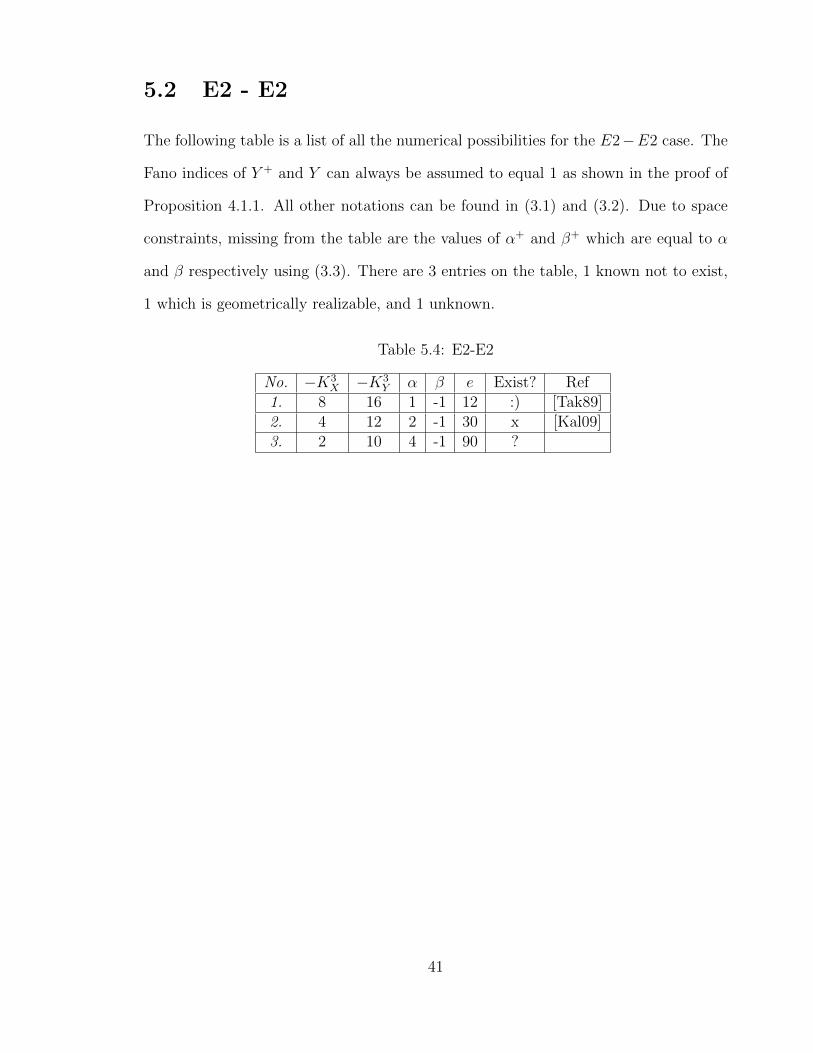
5.2 E2 - E2

The following table is a list of all the numerical possibilities for the E2−E2 case. The

Fano indices of Y + and Y can always be assumed to equal 1 as shown in the proof of

Proposition 4.1.1. All other notations can be found in (3.1) and (3.2). Due to space

constraints, missing from the table are the values of α+ and β+ which are equal to α

and β respectively using (3.3). There are 3 entries on the table, 1 known not to exist,

1 which is geometrically realizable, and 1 unknown.

Table 5.4: E2-E2

No. −K3X −K3

Y α β e Exist? Ref1. 8 16 1 -1 12 :) [Tak89]2. 4 12 2 -1 30 x [Kal09]3. 2 10 4 -1 90 ?

41

5.3 E3/4 - E3/4

The following table is a list of all the numerical possibilities for the E3/4−E3/4 case.

All notation can be found in (3.1) and (3.2). Due to space constraints, missing from

the table are the values of α+ and β+, which are equal to α and β respectively using

(3.3). There are 2 entries on the table, both known to exist.

Table 5.5: E3/4-E3/4

No. −K3X −K3

Y α β e Exist? Ref1. 4 6 1 -1 12 :) [Kal09]2. 2 4 2 -1 24 :) [Puk88]

42

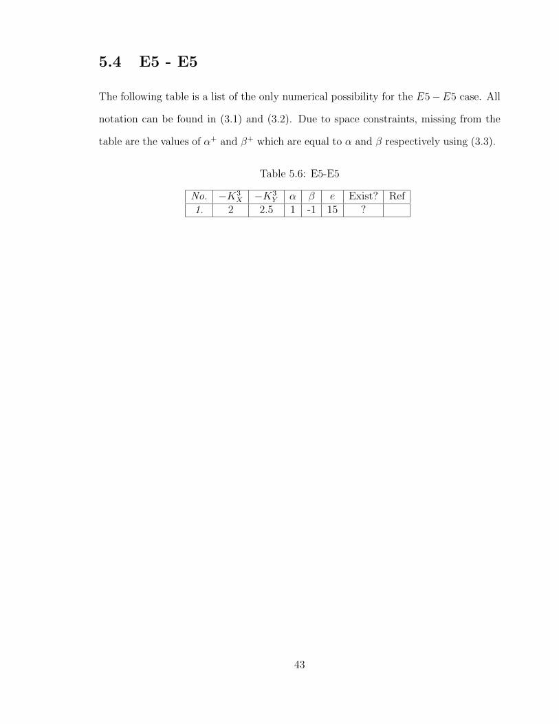
5.4 E5 - E5

The following table is a list of the only numerical possibility for the E5−E5 case. All

notation can be found in (3.1) and (3.2). Due to space constraints, missing from the

table are the values of α+ and β+ which are equal to α and β respectively using (3.3).

Table 5.6: E5-E5

No. −K3X −K3

Y α β e Exist? Ref1. 2 2.5 1 -1 15 ?

43

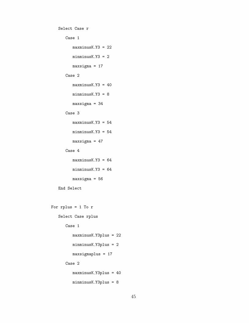
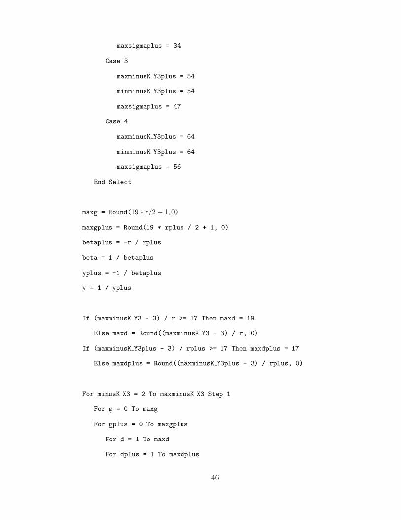
Algorithm Source Code

This program finds all numerical solutions for the E1 − E1 case and was written in

Visual Basic and compiled as a macro in Microsoft Excel. The solutions for the other

symmetric divisorial cases were determined by hand as shown in the corresponding

section in this paper.

Sub E1E1()

Dim rowcounter, r, rplus, minusK X3, minusK Y3, g, d As Integer

Dim sigma, sigmaplus, maxsigma, maxsigmaplus, maxr, maxminusK X3 As Int

Dim minminusK Y3, minminusK Y3plus, maxminusK Y3, maxminusK Y3plus As Int

Dim maxg, maxgplus, maxd, maxdplus As Integer

Dim K X2E, K XE2, K XE2plus, K X2Eplus As Long

Dim y, yplus, k, kplus, x, xplus As Double

Dim e, eplus As Long

Dim alpha, beta, alphaplus, betaplus As Double

Dim K ESquiggle2, K EplusSquiggle2, EPlusSquiggle3, Eplus3 As Double

Dim ESquiggle3, E3 As Double

Dim SheetName As String

Application.ScreenUpdating = False

maxr = 4

maxminusK X3 = 22

rowcounter = 2

SheetName = "E1 - E1"

For r = 1 To maxr

’calculate max values:

44

Select Case r

Case 1

maxminusK Y3 = 22

minminusK Y3 = 2

maxsigma = 17

Case 2

maxminusK Y3 = 40

minminusK Y3 = 8

maxsigma = 34

Case 3

maxminusK Y3 = 54

minminusK Y3 = 54

maxsigma = 47

Case 4

maxminusK Y3 = 64

minminusK Y3 = 64

maxsigma = 56

End Select

For rplus = 1 To r

Select Case rplus

Case 1

maxminusK Y3plus = 22

minminusK Y3plus = 2

maxsigmaplus = 17

Case 2



45

maxsigmaplus = 34

Case 3



maxsigmaplus = 47

Case 4



maxsigmaplus = 56

End Select

maxg = Round(19 ∗ r/2 + 1, 0)

maxgplus = Round(19 * rplus / 2 + 1, 0)

betaplus = -r / rplus

beta = 1 / betaplus

yplus = -1 / betaplus

y = 1 / yplus

If (maxminusK Y3 - 3) / r >= 17 Then maxd = 19

Else maxd = Round((maxminusK Y3 - 3) / r, 0)

If (maxminusK Y3plus - 3) / rplus >= 17 Then maxdplus = 17

Else maxdplus = Round((maxminusK Y3plus - 3) / rplus, 0)

For minusK X3 = 2 To maxminusK X3 Step 1

For g = 0 To maxg

For gplus = 0 To maxgplus

For d = 1 To maxd

For dplus = 1 To maxdplus

46

minusK Y3 = minusK X3 + 2 * r * d - 2 * g + 2

minusK Y3plus = minusK X3 + 2 * rplus * dplus - 2 * gplus + 2

If minusK Y3 > maxminusK Y3 Or minusK Y3 < minminusK Y3

Then GoTo NextdPlusLine

If minusK Y3plus > maxminusK Y3plus

Or minusK Y3plus < minminusK Y3plus


If minusK Y3 Mod r ^ 3 <> 0 Then GoTo NextdPlusLine

If minusK Y3plus Mod rplus ^ 3 <> 0 Then GoTo NextdPlusLine

If minusK Y3 Mod 2 <> 0 Then GoTo NextdPlusLine

If minusK Y3plus Mod 2 <> 0 Then GoTo NextdPlusLine

K XE2 = 2 - 2 * g

K X2E = r * d + 2 - 2 * g

K XE2plus = 2 - 2 * gplus

K X2Eplus = rplus * dplus + 2 - 2 * gplus

sigma = K X2E

sigmaplus = K X2Eplus

If sigma < 0 Or sigma > maxsigma


If sigmaplus < 0 Or sigmaplus > maxsigmaplus


E3 = -1 * r * d + 2 - 2 * g

Eplus3 = -1 * rplus * dplus + 2 - 2 * gplus

alphaplus = (sigma - betaplus * sigmaplus) / minusK X3

47

alpha = -1 * alphaplus / betaplus

K EplusSquiggle2 = (alpha - 1) ^ 2 * alpha * minusK X3

+ (3 * alpha ^ 2 - 4 * alpha + 1) * beta * K X2E

+ (-3 * alpha + 2) * beta ^ 2 * K XE2

+ beta ^ 3 * E3

If sigmaplus < 0 Or sigmaplus > maxsigmaplus


E3 = -1 * r * d + 2 - 2 * g

Eplus3 = -1 * rplus * dplus + 2 - 2 * gplus

alphaplus = (sigma - betaplus * sigmaplus) / minusK X3

alpha = -1 * alphaplus * betaplus

x = y * alpha

xplus = yplus * alphaplus

If Int((x + 1) / y) <> (x + 1) / y Then GoTo NextdPlusLine

If Int((xplus + 1) / yplus) <> (xplus + 1) / yplus


k = (x + 1) / y

kplus = (xplus + 1) / yplus

K EplusSquiggle2 = (alpha - 1) ^ 2 * alpha * minusK X3

+ (3 * alpha ^ 2 - 4 * alpha + 1) * beta * K X2E

+ (-3 * alpha + 2) * beta ^ 2 * K XE2 + beta ^ 3 * E3

K ESquiggle2 = (alphaplus - 1) ^ 2 * alphaplus * minusK X3

+ (3 * alphaplus ^ 2 - 4 * alphaplus + 1)

* betaplus * K X2Eplus

48

+ (-3 * alphaplus + 2) * betaplus ^ 2 * K XE2plus

+ betaplus ^ 3 * Eplus3

EPlusSquiggle3 = alpha ^ 3 * minusK X3

+ 3 * alpha ^ 2 * beta * sigma

- 3 * alpha * beta ^ 2 * K XE2 + beta ^ 3 * E3

ESquiggle3 = alphaplus ^ 3 * minusK X3

+ 3 * alphaplus ^ 2 * betaplus

* sigmaplus - 3 * alphaplus * betaplus ^ 2 * K XE2plus

+ betaplus ^ 3 * Eplus3

e = E3 - ESquiggle3

eplus = Eplus3 - EPlusSquiggle3

If Int(alphaplus * r / betaplus) <> alphaplus * r / betaplus


If Int(alpha * rplus / beta) <> alpha * rplus / beta


If Int((alphaplus + 1) / betaplus) <> (alphaplus + 1) / betaplus


If Int((alpha + 1) / beta) <> (alpha + 1) / beta


If alpha + beta * alphaplus <> 0

Or alphaplus + betaplus * alpha <> 0


If Int(K EplusSquiggle2) <> K EplusSquiggle2


If Int(K ESquiggle2) <> K ESquiggle2 Then GoTo NextdPlusLine

If Int(EPlusSquiggle3) <> EPlusSquiggle3 Then GoTo NextdPlusLine

49

If Int(ESquiggle3) <> ESquiggle3 Then GoTo NextdPlusLine

If Int(alpha - beta) <> (alpha - beta) Then GoTo NextdPlusLine

If Int(alphaplus - betaplus) <> (alphaplus - betaplus)


If Int(r * alpha) <> (r * alpha) Then GoTo NextdPlusLine

If Int(rplus * alphaplus) <> (r * alpha)

Or Int(rplus * betaplus) <> rplus * betaplus


If e <= 0 Or eplus <= 0 Then GoTo NextdPlusLine

’Tests C1-C4:

’C1:

If minusK Y3 <> y ^ 2 * (minusK X3 * k ^ 2

- 2 * k * sigmaplus + 2 * gplus - 2)


’C1+:

If minusK Y3plus <> yplus ^ 2 * (minusK X3 * kplus ^ 2

- 2 * kplus * sigma + 2 * g - 2)


’C2:

If 0 <> minusK X3 * k ^ 2 * x + sigmaplus * (2 * k - 3 * k ^ 2 * y)

+ (2 * gplus - 2) * (3 * k * y - 1) + (rplus * dplus - 2

+ 2 * gplus + eplus) * y


’C2+:

If 0 <> minusK X3 * kplus ^ 2 * xplus + sigma * (2 * kplus

- 3 * kplus ^ 2 * yplus) + (2 * g - 2) * (3 * kplus * yplus - 1)

+ (r * d - 2 + 2 * g + e) * yplus

50


’C3:

If minusK X3 * k * x - sigmaplus * (2 * y * k - 1)

+ (2 * gplus - 2) * y <> r * d / y


’C3+

If minusK X3 * kplus * xplus - sigma * (2 * yplus * kplus - 1)

+ (2 * g - 2) * yplus <> rplus * dplus / yplus


’C4

If minusK X3 * x ^ 2 - 2 * sigmaplus * y * x

+ (2 * gplus - 2) * y ^ 2

- 2 * g + 2 <> 0


’C4+

If minusK X3 * xplus ^ 2 - 2 * sigma * yplus * xplus +

(2 * g - 2) * yplus ^ 2 - 2 * gplus + 2 <> 0


Sheets(SheetName).Cells(rowcounter, 1) = rowcounter - 1

Sheets(SheetName).Cells(rowcounter, 2) = r

Sheets(SheetName).Cells(rowcounter, 3) = rplus

Sheets(SheetName).Cells(rowcounter, 4) = minusK X3

Sheets(SheetName).Cells(rowcounter, 5) = alpha

Sheets(SheetName).Cells(rowcounter, 6) = beta

Sheets(SheetName).Cells(rowcounter, 7) = alphaplus

Sheets(SheetName).Cells(rowcounter, 8) = betaplus

Sheets(SheetName).Cells(rowcounter, 9) = g

51

Sheets(SheetName).Cells(rowcounter, 10) = d

Sheets(SheetName).Cells(rowcounter, 11) = gplus

Sheets(SheetName).Cells(rowcounter, 12) = dplus

Sheets(SheetName).Cells(rowcounter, 13) = minusK Y3

Sheets(SheetName).Cells(rowcounter, 14) = minusK Y3plus

Sheets(SheetName).Cells(rowcounter, 15) = K EplusSquiggle2

Sheets(SheetName).Cells(rowcounter, 16) = K ESquiggle2

Sheets(SheetName).Cells(rowcounter, 17) = EPlusSquiggle3

Sheets(SheetName).Cells(rowcounter, 18) = Eplus3

Sheets(SheetName).Cells(rowcounter, 19) = ESquiggle3

Sheets(SheetName).Cells(rowcounter, 20) = E3

Sheets(SheetName).Cells(rowcounter, 21) = e

Sheets(SheetName).Cells(rowcounter, 22) = eplus

Sheets(SheetName).Cells(rowcounter, 23) = sigma

Sheets(SheetName).Cells(rowcounter, 24) = sigmaplus

rowcounter = rowcounter + 1

NextdPlusLine:

Next dplus

Next d

Next gplus

Next g

Next minusK X3

Next rplus

Next r

Application.ScreenUpdating = True

End Sub

52

Bibliography

[Ba97] V. Batyrev; Stringy Hodge Numbers of Varieties with Gorenstein Canonical Singular-

ities, Integrable Systems and Algebraic Geometry (Kobe/Kyoto, 1997), World Sci. Publ.,

River Edge, NJ (1998), 1-32.

[CM10] J. Cutrone, N. Marshburn; Towards the Completion of Weak Fano Threefolds with

ρ = 2, arXiv:1009.5036v1 [math.AG].

[Cor95] A. Corti; Factoring Birational Maps of Threefolds after Sarkisov, J. Algebraic Ge-

ometry, 4(2):223-254, 1995.

[CG72] C. Clemens, P. Griffiths; The Intermediate Jacobian of the Cubic Threefold, Annals

of Mathematics. Second Series 95 (2): 281356, (1972).

[Ha77] R. Hartshorne; Algebraic Geometry, Graduate Texts in Mathematics, No. 52.

Springer-Verlag, New York - Heidelberg, 1977.

[Isk78] V.A. Iskovskikh; Fano 3-folds I, II, Math USSR, Izv. 11, 485-527 (1977); 12, 469-506

(1978).

[Isk79] V.A. Iskovskikh; Birational Automorphisms of three-dimensional Algebraic Vari-

eties. Current problems in mathematics, VINITI, Moscow, 12, 159-236 (Russian). [English

transl.: J. Soviet Math. 13 (1980) 815-868], Zbl. 428.14017.

[IP99] V.A. Iskovskikh, Yu.G. Prokhorov; Algebraic Geometry V: Fano Varieties, Springer

1999.

53

[JP06] P. Jahnke, T. Peternell; Almost del Pezzo manifolds, arXiv:math/0612516v1

[math.AG].

[JPR05] P. Jahnke, T. Peternell, I. Radloff; Threefolds with Big and Nef AntiCanonical

Bundles I, Math. Ann. 333, No.3, 569-631 (2005).

[JPR07] P. Jahnke, T. Peternell, I. Radloff; Threefolds with Big and Nef AntiCanonical

Bundles II, arXiv:0710.2763v1 [math.AG].

[Kal09] A. Kaloghiros; A Classification of Terminal Quartic 3-Folds and Applications to

Rationality Questions, arXiv:0908.0289v1 [math.AG].

[Ka08] Y. Kawamata; Flops Connect Minimal Models, Publ. RIMS, Kyoto Univ. 44 (2008),

419-423.

[Ko89] J. Kollar; Flops, Nagoya Math. J. 113, 15-36 (1989).

[Mar11] N. Marshburn; Weak Fano Manifolds, (thesis), 2011.

[Mat10] K. Matsuki; Introduction to the Mori Program, Universitext, Springer-Verlag, New

York, 2002.

[Puk88] A.V. Pukhlikov; Birational Automorphisms of a Three-Dimensional Quartic with a

Simple Singularity, Mat. Sb. 135, 472-495 (1988) (Russian). [English transl.: Math. USSR-

SB. 63 (1989) 457-482, Zbl. 668.14007].

[Sar89] V. G. Sarkisov; Birational Maps of Standard Q-Fano Fiberings, I.V. Kurchatov In-

stitute of Atomic Energy preprint, 1989.

[ShC10] V.V. Shokurov, S.R. Choi; Geography of Log Models: Theory and Applications,Cent.

Eur. J. Math. (to appear).

[Shi89] K. Shin; 3-dimensional Fano Varieties with Canonical Singularities, Tokyo J. Math.,

12(2): 375-385, 1989.

54

[Chel06] I. Cheltsov; Nonrational Nodal Quartic Threefolds, Pacific J. Math. 226:1 (2006),

65-82.

[Tak89] K. Takeuchi; Some birational maps of Fano 3-Folds, Compositio Math.,71(3): 265-

283, 1989.

[Tak09] K. Takeuchi; Weak Fano Threefolds with del Pezzo Fibration, arXiv:0910.2188v1

[math.AG].

[Tak02] H. Takagi; On Classification of Q-Fano 3-folds of Gorenstein Index 2, I, II. Nagoya

Math. J., 167:117-155,157-216, 2002.

55

Vitae

Joseph W. Cutrone was born on October 20, 1980 in New Hyde Park, New York. He received

his Bachelor of Science in both mathematics and computer science from Boston College in

May 2002. After college, he worked as a pension actuary in New York, NY for first Segal

and then Towers Perrin until the fall of 2006. In 2003, Joseph was accepted into New York

University’s Courant Institute of Mathematical Sciences and while working full-time, received

his Master of Science in Mathematics in May 2005. He was then accepted into the doctoral

program at Johns Hopkins University starting the fall of 2006. His dissertation was completed

under the guidance of Dr. Vyacheslav Shokurov and was successfully defended on March 14,

2011.

56

Documents

SYMMETRIC SARKISOV LINKS OF FANO THREEFOLDS