SYMMETRIC AND TRIMMED SOLUTIONS OF SIMPLE LINEAR REGRESSION

by

Chao Cheng

A Dissertation Presented to theFACULTY OF THE GRADUATE SCHOOL

UNIVERSITY OF SOUTHERN CALIFORNIAIn Partial Fulfillment of the

Requirements for the DegreeMASTER OF SCIENCE

(STATISTICS)

December 2006

Copyright 2006 Chao Cheng

Dedication

to my grandmother

to my parents

ii

Acknowledgments

First and foremost, I would like to thank my advisor, Dr. Lei Li, for his patience and

guidance during my graduate study. Without his constant support and encouragement,

the completion of the thesis would not be possible. I feel privileged to have had the

opportunity to work closely and learn from him.

I am very grateful to Dr. Larry Goldstein and Dr. Jianfeng Zhang, in the Depart-

ment of Mathematics, for their most valuable help in writing this thesis. Most of my

knowledge about linear regression is learned from Dr. Larry Goldstein’s classes.

I would also like to thank Dr. Xiaotu Ma, Dr. Rui Jiang, Dr. Ming Li, Huanying

Ge, and all the past and current members in our research group for their suggestions and

recommendations. I greatly benefit from the discussion and collaboration with them.

Finally, I would like to thank my little sister and my parents for their love, support

and encouragement. I would also like to thank my grandmother, who passed away in

2002, soon after I began my study in USC. I feel sorry that I did not accompany her in

her last minute. This thesis is dedicated to her.

iii

Table of Contents

Dedication ii

Acknowledgments iii

List of Tables vi

List of Figures vii

Abstract 1

Chapter 1: INTRODUCTION 21.1 Simple linear regression model . . . . . . . . . . . . . . . . . . . . . . 21.2 Least square fitting . . . . . . . . . . . . . . . . . . . . . . . . . . . . 41.3 Robust regression . . . . . . . . . . . . . . . . . . . . . . . . . . . . . 51.4 Least trimmed squares (LTS) . . . . . . . . . . . . . . . . . . . . . . . 7

Chapter 2: Model and algorithm 102.1 Bivariate least squares (BLS) . . . . . . . . . . . . . . . . . . . . . . . 102.2 Solutions of BLS . . . . . . . . . . . . . . . . . . . . . . . . . . . . . 132.3 Bivariate Least Trimmed Squares (BLTS) . . . . . . . . . . . . . . . . 152.4 Algorithm for BPLTS . . . . . . . . . . . . . . . . . . . . . . . . . . . 16

Chapter 3: Mathematical Properties of BLTS Methods 273.1 Symmetry of BLTS methods with respect to x and y . . . . . . . . . . . 273.2 Comparison of BLTS methods . . . . . . . . . . . . . . . . . . . . . . 293.3 Breakdown value of BPLTS method . . . . . . . . . . . . . . . . . . . 323.4 Analysis of multi-component data set using BPLTS . . . . . . . . . . . 343.5 Subset correlation analysis using BPLTS . . . . . . . . . . . . . . . . . 363.6 Scale dependency of BPLTS . . . . . . . . . . . . . . . . . . . . . . . 38

Chapter 4: Application of BPLTS Method to Microarray Normalization 404.1 Introduction to microarray technologies and normalization . . . . . . . 40

iv

4.2 Application of BPLTS to Microarray normalization . . . . . . . . . . . 424.3 Application of SUB-SUB normalization . . . . . . . . . . . . . . . . . 45

References 53

v

List of Tables

3.1 Comparison of different approaches. . . . . . . . . . . . . . . . . . . . 32

3.2 Trimming fraction effect on coefficient estimation using BPLTS. . . . . 34

vi

List of Figures

1.1 Hight of fathers and sons for 14 father-son pairs. The strait line is theleast square fitted line. . . . . . . . . . . . . . . . . . . . . . . . . . . 3

2.1 Illustration of BLS. (A) Ordinary Least Squares (OLS) minimize thesum of vertical distances from (xi, yi) to (xi, yi):

∑(yi − yi)

2. (B)BivariateMultiplicative Least Squares (BMLS) minimize the sum of the areas cir-cled by (xi, yi), (xi, yi) and (xi, yi):

∑ |(yi − yi)(xi − xi)|. (C)BivariateSymmetric Least Squares (BSLS) minimize the sum of summation ofvertical distances from (xi, yi) to (xi, yi) and horizontal distances from(xi, yi) to (xi, yi):

∑[(yi − yi)

2 + (xi − xi2)]. (D)Bivariate Perpendic-

ular Least Squares (BPLS) minimize the the sum of perpendicular dis-tances from (xi, yi) to (xi, yi):

∑(yi − yi)

2 cos2(arctan β). . . . . . . 12

3.1 Fitted regression lines using (A)OLTS (B)BMLTS (C)BSLTS (D)BPLTS.In (A), the magenta and cyan lines are the best fitted lines of regressiony ∼ x and x ∼ y, respectively when OLTS is used. In (B)-(D), the bluepoints are excluded outliers. In (A)-(D), a trimming fraction of 30% isused. . . . . . . . . . . . . . . . . . . . . . . . . . . . . . . . . . . . . 28

3.2 The first simulated data set. (A) OLTS with y ∼ x (B) OLTS with x ∼ y(C) BLTS (D) Ordinary least square fitting. In (A)(B)(C): the trimmingfraction is 20%; the outliers are shown as blue dots. in (D): the dashedlines are from ordinary least squares(red: y ∼ x; green: x ∼ y); thesolid lines are from OLTS (cyan: y ∼ x; purple: x ∼ y) and BLTS(black). . . . . . . . . . . . . . . . . . . . . . . . . . . . . . . . . . . 29

3.3 Comparison of OLTS(A), BMLTS(B), BSLTS(C) and BPLTS(D) usingsimulated data set with errors in both x and y. The magenta stars markthe data points in the h-size subset. The blue dots indicate the outliers. . 30

3.4 Robustness of BPLTS method. The purple “+”s in the bottom left are“outliers”. . . . . . . . . . . . . . . . . . . . . . . . . . . . . . . . . . 33

vii

3.5 Analysis of multi-component data set using BPLTS. (A) Identificationof the first component. The trimming fraction is 20%.(B) Identificationof the second component. The data points in the h-size subset identi-fied by the first BPLTS regression are excluded from the second BPLTSregression. The trimming fraction is 10%. (C)Same as in (A), but thetrimming fraction is 50%. (D)Same as in (B), but the trimming fractionis 40%. The data points from the first and the second component aremarked by blue and cyan dots, respectively. The magenta stars indi-cates the data points in the h-size subset for the corresponding BPLTSregression. . . . . . . . . . . . . . . . . . . . . . . . . . . . . . . . . 35

3.6 Subset correlation analysis using BPLTS. (A) 50%-subset correlationbetween x and y. (B) 50%-subset correlation between y and z. (C)50%-subset correlation between x and z. . . . . . . . . . . . . . . . . 36

3.7 BPLTS is scale dependent. (A) Regression of y on x. (B) Regressionof y on 10x. (C) Regression of 10y on x. (D) Regression of 10y on10x. The magenta stars mark the h-size subset identified by the BPLTSregression. The blue dots are those outliers. . . . . . . . . . . . . . . . 38

4.1 Distribution of log transformed expression measurement. (A) probelevel before SUB-SUB normalization. (B)probe level after SUB-SUBnormalization. (C) gene level before SUB-SUB normalization. (D)genelevel after SUB-SUB normalization. SUB-SUB parameters: windowsize 20× 20; overlapping size 10; trimming fraction: 80%. . . . . . . . 47

4.2 M-A plots of spike-in data after Sub-Sub normalization. The x-axisis the average of log-intensities from two arrays. The y-axis is theirdifference after normalization. (A)trimming fraction is 0. (B)trimmingfraction is 10%. (C)trimming fraction is 20%. (D)trimming fractionis 40%. The red points represent those Spike-in genes. Window size20× 20; Overlapping size: 10. . . . . . . . . . . . . . . . . . . . . . . 48

4.3 The slope matrices of two arrays show different spatial patterns in scale.The common reference is Array M. (A) Array P versus M; (B) Array Nversus M. Their histograms are shown at bottom correspondingly in (C)and (D). . . . . . . . . . . . . . . . . . . . . . . . . . . . . . . . . . . 49

viii

4.4 M-A plots of perturbed spike-in data set after SUB-SUB normalization.The x-axis is the average of log-intensities from two arrays. The y-axisis their difference after normalization. In the top four subplots, 20%randomly selected genes have been artificially up-regulated by 2.5 foldin Array Q, R, S, and T. The differentiated genes are marked red, andundifferentiated genes are marked black. The trimming fractions in thesubplots are: (A) 0%; (B) 10%; (C) 30%; (D) 50%. . . . . . . . . . . . 50

4.5 The lowess curves of |M | versus A values by various normalizationmethods. . . . . . . . . . . . . . . . . . . . . . . . . . . . . . . . . . . 51

ix

Abstract

Least trimmed squares (LTS), as a robust method, is widely used in linear regression

models. However, the ordinary LTS of simple linear regression treats the response and

prediction variable asymmetrically. In other world, it only considers the errors from

response variable. This treatment is not appropriate in some applications. To overcome

these problems, we develop three versions of symmetric and trimmed solutions that take

into consideration errors from both response and predictor variable.

In the thesis, we describe the algorithms to achieve the exact solutions for these three

symmetric LTS. We show that these methods lead to more sensible solutions than ordi-

nary LTS. We also apply one of the methods to the microarray normalization problem. It

turns out that our LTS based normalization method has advantages over other available

normalization methods for microarray data set with large differentiation fractions.

1

Chapter 1

INTRODUCTION

1.1 Simple linear regression model

Regression is a methodology for studying relations between variables, where the rela-

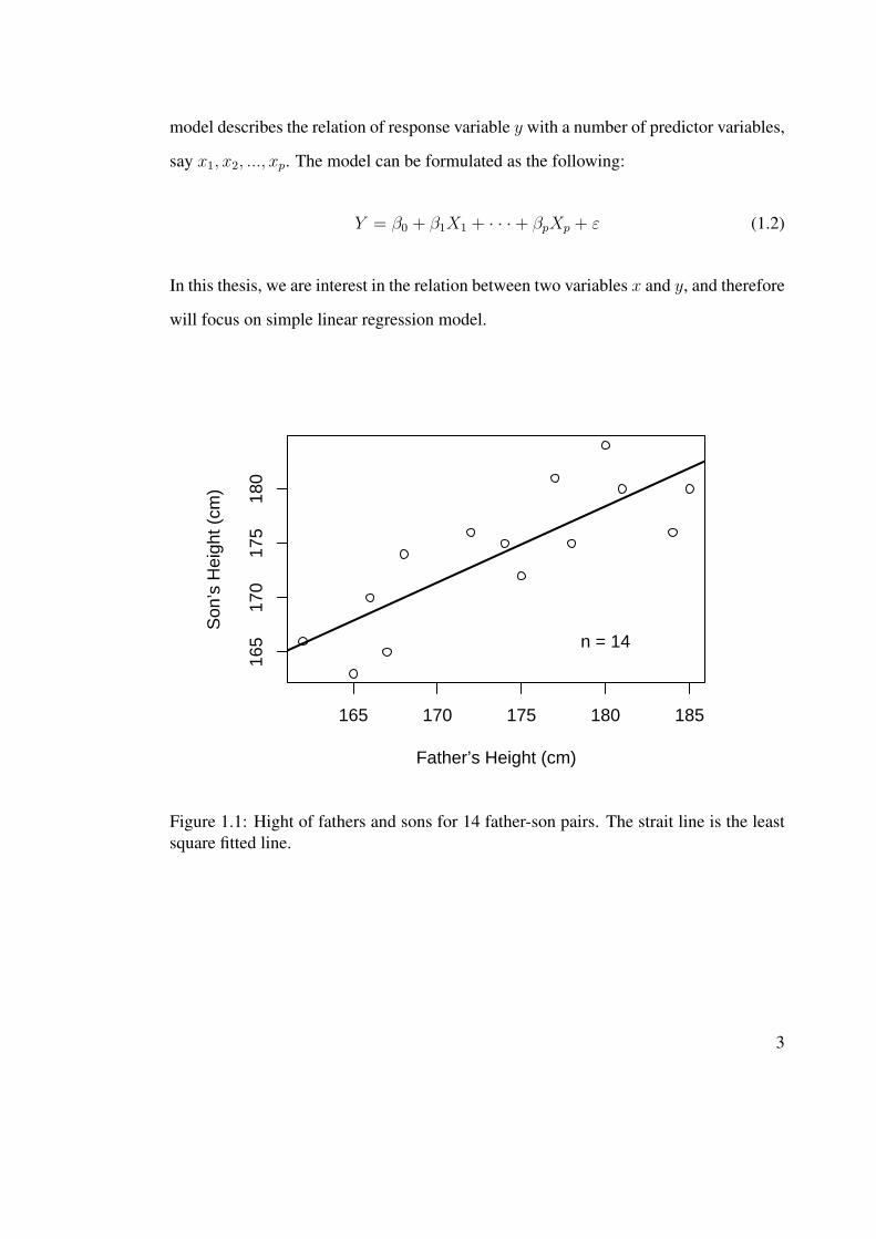
tions are approximated by functions. In the late 1880s, Francis Galton was studying the

inheritance of physical characteristics. In particular, he wondered if he could predict a

boy’s adult height based on the height of his father. Galton hypothesized that the taller

the father, the taller the son would be. He plotted the heights of fathers and the heights

of their sons for a number of father-son pairs, then tried to fit a straight line through the

data (Figure 1.1). If we denote the son’s height by y and the father’s height by x, the

relation between y and x can be described by a simple linear model:

Y = α + βX + ε (1.1)

In the simple linear regression model, y is called dependent variable, x is called

predictor variable, and ε is called prediction error or residual. The symbols α and β are

called regression parameters or coefficients.

Simple linear regression model is a special case of multiple linear regression model,

which involves in more than one predictor variables. i.e., multiple linear regression

2

model describes the relation of response variable y with a number of predictor variables,

say x1, x2, ..., xp. The model can be formulated as the following:

Y = β0 + β1X1 + · · ·+ βpXp + ε (1.2)

In this thesis, we are interest in the relation between two variables x and y, and therefore

will focus on simple linear regression model.

165 170 175 180 185

165

170

175

180

Father’s Height (cm)

Son

’s H

eigh

t (cm

)

n = 14

Figure 1.1: Hight of fathers and sons for 14 father-son pairs. The strait line is the leastsquare fitted line.

3

1.2 Least square fitting

Once a model has been specified, the next task in regression analysis is to fit the model

to the data. For the model (1.1) the task is to find specific values for α and β, to represent

the data as well as possible. As long as α and β have been specified, a specific straight

line can be determined to represent the relation between x and y as shown in Figure

1.1. By far the most important and popular method for doing this is what so called least

square fitting. It aims to find values for α and β that minimize the sum of squares of the

vertical deviations of the data points (x, y) from the fitted straight line. Namely,

(α, β) = arg minα,β

n∑i=1

(yi − yi)2 = arg min

α,β

n∑i=1

(yi − α− βxi)2

The minimizing values α and β are called least squares estimates of α and β or least

squares regression coefficients. The corresponding line is called the least square regres-

sion line. The y , α + βx represents the fitted value calculated from the regression.

Let’s define F (α, β) =∑n

i=1 (yi − α− βxi)2, then we can obtain least squares

regression coefficients α and β by solving the following equations:

∂ F (α, β)

∂ α= 0

∂ F (α, β)

∂ β= 0

(1.3)

The solution is:

β =Sxy

Sxx

α = y − βx(1.4)

where Sxy =∑n

i=1 (xi − x)(yi − y) and Sxx =∑n

i=1 (xi − x)2.

4

It should be note that the regression model itself and the least square fitting is not

symmetric with respect to the predictor variable x and the response variable y. In the

least square fitting, it is the vertical, and not the horizontal deviations that are minimized.

The horizontal deviations should be minimized if we are interested in estimating the

relation of x to y rather than that of y to x. The asymmetry can be rationalized if the

model is used to make prediction. If we are interested in predicting y from x using a

linear relation, we should minimize the vertical deviations∑

(yi − yi)2. On the other

hand, if we want to predict x from y, we should minimize the horizontal deviations∑

(xi − xi)2 and consistently the model X = α + βY + ε should be used.

Sometimes we are interested in estimating the linear relation between x and y rather than

making prediction of one variable from the other. In these cases, x and y are of equal

importance and should be treated symmetrically. Thereby, the least square fitting is not

appropriate to be used any more, because it consider only the errors from the so-called

response variable and the errors from predictor variable are completely ignored. As a

matter of fact, in the canonical simple linear regression model given by model (1.1), only

the response variable y is considered as a random variable, x is regarded as a constant

variable. For the above reasons, the least square regression line estimated using x as

predictor are distinct with the one using y as predictor. This is unreasonable when x and

y are of the same importance and may lead to troubles in practise. We will investigate

this problem in details in latter part.

1.3 Robust regression

One can prove that least squares estimates are the most efficient unbiased estimates of

the regression coefficients under the assumption that the errors are normally distributed.

However, they are not robust to the outliers that are present in the data. To obtain sensible

5

estimates of the regression coefficients in such circumstances, robust regression that are

not sensitive to outliers should be used.

The sensitivity of least squares to outliers is due to two factors [SL03].First, when

the squared residual is used to measure size, any residue with a large magnitude will

have a very large size relative to the others. Second, by using a measure of location

such as mean that is not robust, any large square will have a very strong impact on the

criterion, which will result in the extreme data point having a disproportionate influence

on the regression.

Consistently, we may have two strategies to achieve robust regression. First, we

can replace the square ε2 by some other function ρ(ε), which reflects the size of the

residual in a less extreme way. The idea lead to the notion of M estimation [jH73],S

estimation [RY84], MM estimation [Yoh87] and least absolute value (LAV) regres-

sion [STA01]. As an example, in LAV regression, the regression coefficients are

obtained by minimize∑n

i=1 |yi − α− βxi|. Second, we can replace the sum by a more

robust measure of location such as the median or a trimmed mean, which lead to least

median of squares estimates (LMS) [Rou84, VR99] and least trimmed squares esti-

mates (LTS) [RL99, RD99], respectively. Weighted least squares (WLS) is another

approach that follow this strategy [CR88]. The idea is to assign smaller weights for

observations with larger residuals. In the thesis, we will propose a new algorithm to cal-

culate exact solutions of a revised version of LTS, which takes into account errors from

both predictor and response variables. Thus, we will introduce LTS in the next section.

6

1.4 Least trimmed squares (LTS)

LTS is first proposed by Rousseeuw in 1984 [Rou84]. The breakdown values is often

used to measure the robustness of a method. It is defined as the proportion of contami-

nation (outliers) that a procedure can withstand and still achieve accurate estimates. The

breakdown value of ordinary least squares fitting is1

n, which means one outlier in the

observations may cause incorrect estimation of the regression coefficients. The LTS is

widely used for its high breakdown value and other good properties.

We denote the squared residuals in the ascending order by |r2(α, β)|(1) ≤|r2(α, β)|(2) ≤ · · · |r2(α, β)|(n), where r(α, β) = y − α− βx Then the LTS estimate of

coverage h is obtained by

arg minα,β

h∑i=1

|r2(α, β)|(i) .

This definition implies that observations with the largest residuals will not affect the

estimate. The LTS estimator is regression, scale, and affine equivariant; see Lemma 3,

Chapter 3 in Rousseeuw and Leroy [RL99]. In terms of robustness, we can roughly

achieve a breakdown point of ρ by setting h = [n(1 − ρ)] + 1. In terms of efficiency,√

n-consistency and asymptotic normality similar to M-estimator exist for LTS under

some conditions; see Vısek for example [V96, V00]. Despite its good properties, the

computation of LTS remains a problem.

The problem of computing the LTS estimate of α and β is equivalent to search-

ing for the size-h subset(s) whose least squares solution achieves the minimum of

trimmed squares. The total number of size-h subsets in a sample of size n is(

nh

).

A full search through all size-h subsets is impossible unless the sample size is small.

Several ideas have been proposed to compute approximate solutions. First, instead of

exhaustive search we can randomly sample size-h subsets. Second, Rousseeuw and

7

Van Driessen [RD99] proposed a so-called C-step technique (C stands for “concentra-

tion”). That is, having selected a size-h subset, we apply the least squares estimator

to them. Next for the estimated regression coefficients, we evaluate residuals for all

observations. Then a new size-h subset with the smallest squared residuals is selected.

This step can be iterated starting from any subset. In the case of estimating a loca-

tion parameter, Rousseeuw and Leroy [RL99], described a procedure to compute the

exact LTS solution. Rousseeuw and Van Driessen [RD99] applied this idea to adjust

the intercept in the regression case. The idea of subset search is also relevant to LMS;

see Hawkins [Haw93]. Hossjer described an algorithm for computing the exact least

trimmed squares estimate of simple linear regression, which requires O(n3 log n) com-

putations and O(n2) storage [H95]. A refined algorithm, which requires O(n2 log n)

computations and O(n) storage, was also sketched. However, Hossjer remarked that the

refined algorithm is not stable.

Li introduced an algorithm that computes the exact solution of LTS for simple linear

regression with constraints on the slope [Li05]. The idea is to divide the range of slope

into regions in such a way that within each region the order of residuals is unchanged.

As a result, the search for LTS within each such region becomes a problem of linear

complexity. Without constraints, the overall complexity of the algorithm is O(n2 log n)

in time and O(n2) in storage. In practical regression problems, constraints are often

imposed on slopes, which will reduce computing load substantially. Like the canonical

least squares fitting, this algorithm is asymmetric with respect to predictor and response

variable in a way that only errors from response variable are considered. In practice, we

are often need to study the relation between two variables that are of equal importance

and errors from both should be taken into account. In this thesis we will introduce three

algorithms which are developed from Li’s method. The new methods take into account

8

errors from both predictor variable x and response variable y by considering both of

them as random variables.

9

Chapter 2

Model and algorithm

2.1 Bivariate least squares (BLS)

Let us consider a error-in-variables version of simple linear regression model which

regards both of the two variables as random. Suppose we have n independent observa-

tions (xi, yi), i = 1, ..., n, and the underlying linear relation between x and y is

µyi= α + βµxi

, i = 1, 2, ..., n.

In each observation, we have:

xi = µxi+ εxi

,

yi = µyi+ εyi

.(2.1)

We assume equal precisions of measurement for both xi and yi at all observations, i.e.

εx1 , εx2 , · · · , εxn and εy1 , εy2 , · · · , εyn are independently and identically distributed. To

calculate the regression coefficient estimates, the ordinary least squares (OLS) fitting

minimize the following target function (Figure 2.1A):

(α, β) = arg minα,β

n∑i=1

(yi − yi)2 = arg min

α,β

n∑i=1

(yi − α− βxi)2

10

To simplify the formulas in later sections, we define:

Sxx =∑n

i=1 (xi − x)2,

Syy =∑n

i=1 (yi − y)2,

Sxy =∑n

i=1 (xi − x)(yi − y),

The solution for OLS is:

β = Sxy/Sxx,

α = y − βx.

In order to take into account errors from both x and y, we need construct a target

function that is symmetric with respect to x and y. Three possible target functions can

be used to achieve such a purpose:

(1) (α, β) = arg minα,β

∑ni=1 |(yi − yi)(xi − xi)|

= arg minα,β

∑ni=1

(yi − α− βxi)2

|β|

(2) (α, β) = arg minα,β

∑ni=1 [(yi − yi)

2 + (xi − xi2)]

= arg minα,β

∑ni=1 (1 + 1

β2 )(yi − α− βxi)2

(3) (α, β) = arg minα,β

∑ni=1 [(yi − yi)

2 cos2(arctan β)]

= arg minα,β

∑ni=1

(yi − α− βxi)2

1 + β2

In (1), we aims to minimize the sum of the areas circled by (xi, yi), (xi, yi) and

(xi, yi):∑ |(yi − yi)(xi − xi)|, so we define the method as Bivariate Multiplicative

11

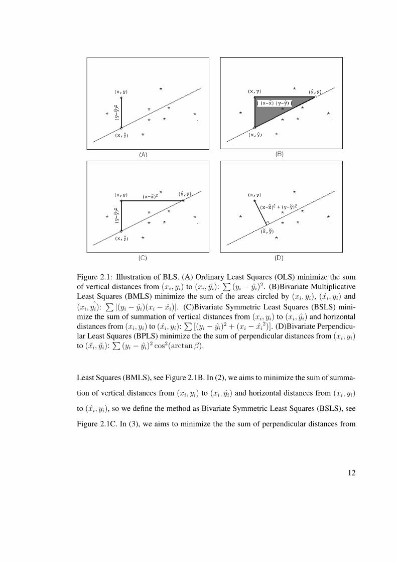
Figure 2.1: Illustration of BLS. (A) Ordinary Least Squares (OLS) minimize the sumof vertical distances from (xi, yi) to (xi, yi):

∑(yi − yi)

2. (B)Bivariate MultiplicativeLeast Squares (BMLS) minimize the sum of the areas circled by (xi, yi), (xi, yi) and(xi, yi):

∑ |(yi − yi)(xi − xi)|. (C)Bivariate Symmetric Least Squares (BSLS) mini-mize the sum of summation of vertical distances from (xi, yi) to (xi, yi) and horizontaldistances from (xi, yi) to (xi, yi):

∑[(yi − yi)

2 + (xi − xi2)]. (D)Bivariate Perpendicu-

lar Least Squares (BPLS) minimize the the sum of perpendicular distances from (xi, yi)to (xi, yi):

∑(yi − yi)

2 cos2(arctan β).

Least Squares (BMLS), see Figure 2.1B. In (2), we aims to minimize the sum of summa-

tion of vertical distances from (xi, yi) to (xi, yi) and horizontal distances from (xi, yi)

to (xi, yi), so we define the method as Bivariate Symmetric Least Squares (BSLS), see

Figure 2.1C. In (3), we aims to minimize the the sum of perpendicular distances from

12

(xi, yi) to (xi, yi):∑

(yi − yi)2 cos2(arctan β), so we define the method as Bivariate

Perpendicular Least Squares (BPLS), see Figure 2.1D.

We note that BPLS has been introduced previously as Total Least Squares (TLS)

together with Error-In-variables model (EIV) [vHL02]. A similar method to BSLS has

also been proposed which minimize the following equation with respect to α and β.

χ2(α, β) =N∑

i=1

(yi − α− βxi)2

σ2yi

+ β2σ2xi

where σxiand σyi

are, respectively, the x and y standard deviations for the ith

point [WBS99]. In this thesis, we would derive several algorithms that are robust

to outliers to solve linear regression problems based on these Bivariate Least Squares

(BLS) methods.

2.2 Solutions of BLS

In this section, we will use the Bivariate Perpendicular Least Squares (BPLS) as example

to show how to solve the three types of Bivariate Least Square fitting. Let us define the

target function for BPLS as:

F (α, β) =n∑

i=1

(yi − α− βxi)2

1 + β2

To achieve the least square estimates α and β, we aim to find the (α, β) that minimize

the function, namely:

(α, β) = arg minα,β

n∑i=1

(yi − α− βxi)2

1 + β2

13

By solving the following equation:

∂ F (α, β)

∂ α= 0

∂ F (α, β)

∂ β= 0

we obtain two solutions:

β = −B ±√B2 + 1

α = y − βx

where B =1

2

[∑n

i=1 x2i − nx2]− [

∑ni=1 y2

i − ny2]∑ni=1 xiyi − nxy

=1

2

Sxx − Syy

Sxy

.

Then we calculate the second order derivatives: A(α, β) , ∂2 F (α, β)

∂ α2, U(α, β) ,

∂2 F (α, β)

∂ β2, and C(α, β) , ∂2 F (α, β)

∂ α ∂ β. As we know, the solution (α, β) that achieve

the minimum of the target function has to satisfy the following inequations: A > 0,

C > 0 and U2 − AC < 0. After calculation, we can prove that only one of the two

solutions achieve the minimum of the target function [Wei]:

β = −B +√

B2 + 1, ifSxy ≥ 0

β = −B −√B2 + 1, ifSxy < 0

.

14

Above is the solution for BPLS, similarly we obtain the solutions for BMLS and

BSLS. For the BMLS we have:

β = ±√Syy/Sxx, ifSxy ≥ 0, take′′+′′; ifSxy < 0, take′′−′′,

α = y − βx.

For the BSLS we have α = y − βx and β can be obtained by solving the following

quartic equation: β4Sxx − β3Sxy + βSxy − Syy = 0. It is hard to derive the formula

solutions for above quartic equation. But we can obtain the numeric solutions by using

various method such as Ferrari’s method [Qua]. Generally, the quartic equation has four

roots, including real roots and imaginary roots. The solution for β is the real root that

minimize the target function.

2.3 Bivariate Least Trimmed Squares (BLTS)

Least Trimmed Squares (LTS) is one of the most frequently used robust regression

method. Several algorithms have been introduced for LTS such as fast-LTS [RD99].

Recently Li et al proposed a new algorithm to compute exact solution of LTS for simple

linear regression [Li05]. In this thesis, we take into account the experimental errors from

both x and y by using the above introduced target functions (BMLS, BSLS and BPLS)

for least squares estimation. Consistently, we designed three bivariate least trimmed

squares algorithms, which are called BMLTS, BSLTS, and BPLTS, respectively. In the

following section, we will describe the algorithm using BPLTS as example. The algo-

rithms of BMLTS and BSLTS are similar to BPLTS.

15

2.4 Algorithm for BPLTS

We consider a simple linear regression problem with a response variable y and an

explanatory variable x. Let (xi, yi), i = 1, · · · , n, be data.

Proposition 1. Consider a simple linear regression with restricted slope range, namely,

we impose a constraint on the slope: β ∈ [b1, b2]. Denote the unrestricted least squares

solution by (α, β).

• If β ∈ [b1, b2], then the unrestricted solution is also the restricted solution.

• If β /∈ [b1, b2], then the restricted solution of the slope is either b1 or b2.

Proof: If β ∈ [b1, b2], then the unrestricted solution satisfies the requirement. Oth-

erwise, according to the Kuhn-Tucker condition, the solution must be on the boundary;

see Luenberger [Lue87] and Lawson and Hanson [LH74]. Stark and Parker provided

another algorithm for the problem of bounded-variable least squares [SP95].

16

Hereafter we refer to any subset of the data by the set of their indices. For the sake of

completeness and convenience, we write down the formulas of the least squares estimate

for any size-h subset H .

xH = 1h

∑i∈H xi ,

yH = 1h

∑i∈H yi ,

xxH = 1h

∑i∈H x2

i ,

yyH = 1h

∑i∈H y2

i ,

xyH = 1h

∑i∈H xiyi ,

cxyH = xyH − xHyH ,

βH = cxyH/[xxH − x2H ] ,

αH = yH − βHxH ,

SSH = [yyH − y2H ]− βHcxyH .

(2.2)

The last quantity is the averaged sum of squares. cxyH represents the centerized version

of xyH . To proceed, we need some notation and definitions.

Definition 1. For any (α, β),

1. Their residuals are defined by r(α, β)i = yi − (α + β xi);

2. H(α,β) is a size-h index set that satisfies the following property: |r(α, β)i| ≤|r(α, β)j|, for any i ∈ H(α,β) and j 6∈ H(α,β).

On the other hand, given any size-h subset H , we can find the least squares estimate

(αH , βH) for the subsample {(xi, yi), i ∈ H}. Thus we have established a correspon-

dence between the parameter space and the collection of all size-h subsets. This leads to

17

our following definition of LTS. Please notice that we consider a general case with pos-

sible constraints on the slope. For convenience, hereafter in this section we use coverage

h instead of a trimming fraction. The breakdown value for coverage h is n−hn

.

Definition 2. For a given coverage h, the least trimmed squares estimate subject to

b1 ≤ β ≤ b2, where −∞ ≤ b1 < b2 ≤ ∞, is defined by

1. (α, β) that minimizes∑

i∈H(α,β)r(α, β)2

i subject to b1 ≤ β ≤ b2;

2. or equivalently, the least squares estimate (αH , βH) of a size-h subset H that

minimizes SSH subject to b1 ≤ βH ≤ b2; cf. (2.2).

Namely, we can either search in the parameter space, or search in the space of size-h

subsets. This dual form of the BPLTS solution is the key to the development of the

algorithms in this paper.

Proposition 2. For any parameter (α, β), we sort its residuals in the ascending order,

namely, r(α, β)π(1) ≤ r(α, β)π(2) ≤ · · · ≤ r(α, β)π(n), where {π(1), π(2), · · · , π(n)} is

a permutation of {1, 2, · · · , n}. Then H(α,β) must be from the n− h + 1 size-h subsets:

{π(k), π(k + 1), · · · , π(k + h− 1)}, k = 1, · · · , n− h + 1.

Proof: This is true because of the following fact: after taking absolute values, one

or more residuals become the smallest; As moving away from the smallest, residuals

increase monotonically leftwards or rightwards.

The significance of the result is that the complexity for the search of H(α,β) reduces

to O(n) from(

nh

). We notice that for fixed β, the order of residuals keeps unchanged

whatever intercept α is chosen. This leads to the following definition.

18

Definition 3. For a fixed β, denote r(β)i = yi − β xi. Let r(β)(i), i = 1, · · · , n, be

their ordered residuals. Their partial ordered averages and partial sums of squares are

defined by:

r(β)(l:m) = 1m−l+1

∑mk=l r(β)(k) ,

SS(β)(l:m) = 1m−l+1

∑mk=l (r(β)(k) − r(β)(l:m))

2, 1 ≤ l ≤ m ≤ n .

(2.3)

This structure and Proposition 2 are the basis of the following algorithm for comput-

ing the BPLTS estimate of a location parameter; see Page 171–172 in Rousseeuw and

Leroy [RL99].

Definition 4. For {yi, i = 1, · · · , n}, we define partial ordered averages and partial

sums of squares respectively by

y(l:l+h−1) =Pl+h−1

k=l y(k)

h,

SS(l:l+h−1) =Pl+h−1

k=l [y(k)−y(l:l+h−1)]2

h.

Corollary 1. The BPLTS estimate of the location of {yi, i = 1, · · · , n} is given by the

partial ordered average(s) that achieves the smallest among SS(l:l+h−1), l = 1, · · · , n−h + 1. In case there are ties, the solution is not unique.

This case corresponds to β = 0 in the simple linear regression. Proposition 2 implies

that we only need to check n− h + 1 partial ordered averages for searching the BPLTS

estimate of the location. Partial ordered averages and sums of squares can be calculated

in a recursive way; see Rousseeuw and Leroy (1987). Go back to the case of simple

linear regression. The next result is the basis of our algorithms.

19

Proposition 3. Suppose that for β ∈ [b1, b2], the order of {r(β)i} keeps unchanged.

Namely, there exists a permutation {π(1), π(2), · · · , π(n)} such that r(β)π(1) ≤r(β)π(2) ≤ · · · ≤ r(β)π(n) for any β ∈ [b1, b2].

• Then the size-h subset(s) for the BPLTS must be from the n− h + 1 subsamples:

{π(k), π(k + 1), · · · , π(k + h− 1)}, where k = 1, · · · , n− h + 1.

• Moreover, for each subsample {π(k), π(k + 1), · · · , π(k + h − 1)}, we compute

its regular least squares estimate denoted by β(k:k+h−1). Then the BPLTS estimate

of β subject to the constraint β ∈ [b1, b2] must be from the following: 1. {b1, b2};

2. or {β(k:k+h−1), satisfying b1 < β(k:k+h−1) < b2, k = 1, · · · , n− h + 1}.

Proof: Let (α, β) be one solution. According to the assumption, we have r(β)π(1) ≤r(β)π(2) ≤ · · · ≤ r(β)π(n). Using the same argument leading to Proposition 2, we

conclude that the size-h subset H(α,β) must be from the n − h + 1 size-h subsets:

{π(k), π(k + 1), · · · , π(k + h− 1)}, k = 1, · · · , n− h + 1. Then we apply Proposition

1 to the subset H(α,β) and the proof is completed. According to this result, we only need

to check the sum of squares for the n− h + 1 candidates subject to the constraint.

Our next move is to divide the range of β into regions in such a way that within each

region the order of residuals is unchanged and thus we can apply the above proposition.

It is motivated by two technical observations. First we consider straight lines connecting

each pair {(xi, yi), (xj, yj)} satisfying (xi, yi) 6= (xj, yj). The total number of such

pairs is at most n(n−1)2

. The regions defined by these dividing lines satisfy the above

order condition. Second, to compute the least squares estimates for the n− h + 1 size-h

subsets within each region, we do not have to repeatedly apply Formulas (2.2). Instead,

from one region to the next, we only need to update estimates if a few residuals change

their orders. The algorithm can be described as the following.

20

1. For any pair (i, j) such that xi 6= xj , compute b(i,j) =yj−yi

xj−xi. Sort {b(i,j)} in the

range [b1, b2] and denote them by b1 < b[1] ≤ b[2] ≤ · · · ≤ b[L] < b2, where

L ≤ n(n−1)2

. Save the pairs of indices corresponding to these slopes.

Remark: Here we exclude all the slopes outside (b1, b2) when sorting slopes. We

first restrict the scope of this algorithm to the case without slope ties, namely:

b1 < b[1] < b[2] < · · · < b[L] < b2. To avoid slope ties, we perturb the original data

by adding a tiny random number to each x′s and y′s before computing pairwise

slope b(i,j). We have a complex version of algorithm which can deal with slope

ties without perturbing the data [Li05]. In this paper, we only show the simple

version considering its efficiency.

2. If b1 = −∞, go to Step 3. If b1 > −∞, then we consider the residuals along the

lower bound.

(a) Compute r(b1)i = yi− b1 xi, i = 1, · · · , n. Sort them in the ascending order

and denote the ordered residuals by {r(b1)(i), i = 1, · · · , n}.

(b) Compute the following quantities, for l = 1, · · · , n− h + 1,

r(b1)(l:l+h−1) = 1h

∑l+h−1k=l r(b1)(k) ,

rr(b1)(l:l+h−1) = 1h

∑l+h−1k=l r(b1)

2(k) ,

SS(b1)(l:l+h−1) =1

1 + b21

[rr(b1)(l:l+h−1) − r(b1)2(l:l+h−1)],

(2.4)

by the recursion

r(b1)(l+1:l+h) = r(b1)(l:l+h−1) + 1h[r(b1)(l+h) − r(b1)(l)] ,

rr(b1)(l+1:l+h) =1

1 + b21

{rr(b1)(l:l+h−1) + 1h[r(b1)

2(l+h) − r(b1)

2(l)]} .

(2.5)

21

(c) Save the size-h subset(s) that achieves the minimum of sum of squares.

3. Take a value β such that b1 < β < b[1].

(a) Compute r(β)i = yi − β xi, i = 1, · · · , n. Sort them in the ascend-

ing order. For ties, we arrange them in the ascending order of x-

values. We denote the ordered residuals by r(β)π(i), i = 1, · · · , n, where

{π(1), π(2), · · · , π(n)} is a permutation of {1, 2, · · · , n}. We also denote

the inverse of {π(1), π(2), · · · , π(n)} by {λ(1), λ(2), · · · , λ(n)}.

(b) Compute the following quantities, for l = 1, · · · , n− h + 1,

x(l:l+h−1) = 1h

∑l+h−1i=l xπ(i) ,

y(l:l+h−1) = 1h

∑l+h−1i=l yπ(i) ,

xx(l:l+h−1) = 1h

∑l+h−1i=l x2

π(i) ,

yy(l:l+h−1) = 1h

∑l+h−1i=l y2

π(i) ,

xy(l:l+h−1) = 1h

∑l+h−1i=l xπ(i)yπ(i) ,

cxy(l:l+h−1) = xy(l:l+h−1) − x(l:l+h−1) y(l:l+h−1) ,

B(l:l+h−1) =[xx(l:l+h−1) − x2

(l:l+h−1)]− [yy(l:l+h−1) − y2(l:l+h−1)]

2cxy(l:l+h−1)

,

β(l:l+h−1) = ±√

B2(l:l+h−1) + 1−B(l:l+h−1)

(if cxy(l:l+h−1) ≥ 0 take ′+′, esle take ′−′),

α(l:l+h−1) = y(l:l+h−1) − β(l:l+h−1)x(l:l+h−1) ,

SS(l:l+h−1) =1

1 + β2{[yy(l:l+h−1) − y2

(l:l+h−1)]− 2β(l:l+h−1)cxy(l:l+h−1)

+β2(l:l+h−1)[xx(l:l+h−1) − x2

(l:l+h−1)]} ,

(2.6)

22

by the recursion

x(l+1:l+h) = x(l:l+h−1) + 1h[xπ(l+h) − xπ(l)] ,

y(l+1:l+h) = y(l:l+h−1) + 1h[yπ(l+h) − yπ(l)] ,

xx(l+1:l+h) = xx(l:l+h−1) + 1h[x2

π(l+h) − x2π(l)] ,

yy(l+1:l+h) = yy(l:l+h−1) + 1h[y2

π(l+h) − y2π(l)] ,

xy(l+1:l+h) = xy(l:l+h−1) + 1h[xπ(l+h)yπ(l+h) − xπ(l)yπ(l)] .

(2.7)

(c) Update the BPLTS solution.

4. For k = 1, 2, · · · , L, do the following.

(a) Consider b[k] and the corresponding pair of indices (i, j). Update the permu-

tation π by letting π(λ(i)) = j and π(λ(j)) = i, and update λ by swapping

λ(i) and λ(j).

(b) Update the quantities in (2.6).

(c) Update the BPLTS solution.

5. If b2 < ∞, go through Step 2, replace b1 by b2, and update the BPLTS solution.

Proposition 4. The output of the above Algorithm is the BPLTS solution.

Proof: First, subject to the constraint b1 < β < b[1], r(β)π(1) ≤ r(β)π(2) ≤ · · · ≤r(β)π(n) is always true for the permutation {π(1), π(2), · · · , π(n)}. Otherwise, we can

find two indices (i, j) such that yi− β xi < yj − β xj for some β values and yi− β xi >

yj − β xj for some other β values. Then there exists at least one value b ∈ (b1, b[1]) such

that yi − b xi = yj − b xj and xi 6= xj . This leads to b =yj−yi

xj−xi, a contradiction to the

assumption that no other b(i,j) exists between b1 and b[1]. Hence we can apply Proposition

23

3 to the interval [b1, b[1]]. As a consequence, we only need to check the n − h + 1 sub-

sample {π(l), π(l + 1), · · · , π(l + h − 1)}, where 1 ≤ l ≤ n − h + 1. This is exactly

Step 2. Next we consider the order structure as β reaches b[1]. Remember that we have

assumed b[1] < b[2]. As β passes b[1] into the interval (b[1], b[2]), the order structure is

preserved except for the pair of indices (i, j) such that b(i,j) =yj−yi

xj−xi= b[1]. Otherwise,

a self-contradiction would occur by the same argument as in the interval (b1, b[1]). If we

do the swap as in Step 4(a): π(λ(i)) = j and π(λ(j)) = i, and exchange λ(i) and λ(j),

then the residuals under the new permutation π are still in the ascending order subject

to b[1] ≤ β < b[2]. Next we update the quantities in (2.6) and apply Proposition 3 to this

region. Recursively, we rotate the slope around the origin and repeat this procedure for

each region b[k] ≤ β < b[k+1].

Proposition 3 guarantees that we can find the size-h subset(s) for the optimal solution

at the end of search. Next we evaluate the complexity of the algorithm. This requires a

more detailed picture of the order structure.

Proposition 5. If we assume that

1. Data contain no identical observations.

2. No tie exists in the slopes {b[l]}, namely, b1 < b[1] < b[2] < · · · < b[L] < b2.

Then

• as β goes from an interval [b[k−1], b[k]) to the next [b[k], b[k+1]), the pair of indices

(ik, jk) involved in the swap, cf. Step 4(a) of the algorithm, must be adjacent to

one another in the permutations π in the two intervals [b[k−1], b[k]) and [b[k], b[k+1]);

• Consequently, we only need to adjust two partial regressions given in Equation

(2.6) and thus the complexity of the algorithm is quadratic in time except for the

part of sorting {b(i,j)}.

24

Proof: When β ∈ [b[k−1], b[k]), we have either yik − β xik < yjk− β xjk

or yik −β xik > yjk

− β xjk. Without loss of generality, we assume the former is true. That is,

yik − β xik < yjk− β xjk

, b[k−1] < β < b[k] ,

yik − β xik = yjk− β xjk

, β = b[k] ,

yik − β xik > yjk− β xjk

, b[k] < β < b[k+1] .

Suppose we have another term (xu, yu) whose residual is between these two terms for

β ∈ [b[k−1], b[k]). That is, yik − β xik < yu − β xu < yjk− β xjk

. This implies

0 < (yu − yik)− β (xu − xik) < (yjk− yik)− β (xjk

− xik) .

When β −→ b[k] , we have

0 ≤ (yu − yik)− β (xu − xik) ≤ (yjk− yik)− β (xjk

− xik) = 0 .

Hence we have yu−yik = β (xu−xik) and b[k] =yu−yik

xu−xik. This conflicts the assumption.

Similarly, the two terms indexed by ik, jk are still next to each other in the interval

[b[k], b[k+1]). The only change in π is the swap of their positions. This exchange involves

only two partial regressions given in (2.6).

It should be note that the above algorithm gives the exact solution only if there is

no tie exists in the slope b(i,j)’s. In practise, we can avoid slope tie by introducing

tiny random perturbations to the data points (xi, yi), namely, we add a tiny random

number to each xi or yi. In addition, we also have a version of algorithm that can deal

with general case in which ties may occur in b(i,j)’s. But it is not as efficient as the

above simple version in terms of time complexity. Further more, we find that the simple

25

version can obtain almost the same result as the general version, if random perturbation

is performed. So in the thesis, we always use the results from the simple version.

26

Chapter 3

Mathematical Properties of BLTS

Methods

3.1 Symmetry of BLTS methods with respect to x and y

The target function of ordinary least trimmed squares (OLTS) only considers the errors

from response variable. Regression of y on x (y ∼ x) and regression of x on

y (x ∼ y) will give distinct h-size subset and regression line. On the other hand, the

target functions for bivariate multiplicative least trimmed squares (BMLTS), bivariate

symmetric least trimmed squares (BSLTS), and bivariate perpendicular least trimmed

squares (BPLTS) are all symmetric with respect to x and y. Therefore, regression y ∼ x

and x ∼ y will result in the same h-size subsets and regression lines. We applied OLTS,

BMLTS, BSLTS, and BPLTS regression with both y ∼ x and x ∼ y to a data with 200

points, the result is show in Figure 3.1. The trimming fraction for all the LTS are set to

30%. The OLTS lead to two distinct regression lines corresponding to y ∼ x and x ∼ y,

as shown in Figure 3.1A. While the other three bivariate least trimmed squares (BMLTS,

BSLTS and BPLTS) achieve the same result for y ∼ x and x ∼ y, as shown in Figure

3.1B-D.

Figure 3.2 shows the results of ordinary least squares (OLS), OLTS and BPLTS

using the same data set. This time a trimming fraction of 20% are used. As can be

seen, the h-size subsets of y ∼ x (Figure 3.2A) and x ∼ y (Figure 3.2B) identified by

OLTS are different with each other. In Figure 3.2D, the regression lines by OLS are

27

1800 2000 2200 2400 2600 2800

2000

3000

4000

5000

(A)1800 2000 2200 2400 2600 2800

2000

3000

4000

5000

(B)

1800 2000 2200 2400 2600 2800

2000

3000

4000

5000

(C)1800 2000 2200 2400 2600 2800

2000

3000

4000

5000

(D)

y = 488.65+0.85xx = 803.79+0.58y

y = −360.62+1.25x

y = −229.89+1.19x y = −482.62+1.30x

Figure 3.1: Fitted regression lines using (A)OLTS (B)BMLTS (C)BSLTS (D)BPLTS. In(A), the magenta and cyan lines are the best fitted lines of regression y ∼ x and x ∼ y,respectively when OLTS is used. In (B)-(D), the blue points are excluded outliers. In(A)-(D), a trimming fraction of 30% is used.

shown as dashed lines. Since OLS estimate the correlation coefficients based on all the

data points without trimming, it will affected by the outliers in the data. As shown, the

regression lines of y ∼ x and x ∼ y by OLS are more different in comparison with those

by OLTS. Despite the difference, all the LTS methods give more reliable estimation of

the regression coefficients than the OLS method.

28

y = 0.85x + 488.65

(A)

x = 0.58y + 803.79

(B)

y = 1.30x − 482.62

(C)

y = 1.22x − 100.38x = 0.29y + 1462.05

(D)

Figure 3.2: The first simulated data set. (A) OLTS with y ∼ x (B) OLTS with x ∼ y(C) BLTS (D) Ordinary least square fitting. In (A)(B)(C): the trimming fraction is 20%;the outliers are shown as blue dots. in (D): the dashed lines are from ordinary leastsquares(red: y ∼ x; green: x ∼ y); the solid lines are from OLTS (cyan: y ∼ x; purple:x ∼ y) and BLTS (black).

3.2 Comparison of BLTS methods

We then investigate the accuracy of OLTS and our three BLTS methods for estimate

linear relation between two variables. When we estimate the relation between father’s

height and son’s height, we measure the height of all the father-son pairs. Certainly, we

would expect experiment errors for both father’s height and son’s height. However, the

OLS and OLTS only take in consideration the errors from the response variable, that is,

the errors from the father’s height when regress father’s height on son’height. The three

29

0 500 1000−500

0

500

1000y = 274.45+0.4970x

(A)0 500 1000

−500

0

500

1000y = 71.60+0.8908x

(B)

0 500 1000−500

0

500

1000y = 41.70+0.9349x

(C)0 500 1000

−500

0

500

1000y = 109.63+0.8027x

(D)

Figure 3.3: Comparison of OLTS(A), BMLTS(B), BSLTS(C) and BPLTS(D) using sim-ulated data set with errors in both x and y. The magenta stars mark the data points inthe h-size subset. The blue dots indicate the outliers.

methods BMLTS, BSLTS and BPLTS we propose in the thesis consider errors from

both variables. As such, we may expect a more accurate estimation of the linear relation

between the two variables. To investigate this problem, we simulate a data set of size

1000 using the following procedure. First, we generate a vector X = [1, 2, ..., 1000],

Second we generate another vector Y , where Yi = 100 + 0.8Xi, i = 1, 2, ..., 1000.

Finally, we introduce errors for both X and Y by adding a random number εx or εy

for each Xi and Yi, where εx ∼ (0, 200), and εy ∼ (0, 200). That is for the 1000

observations (xi, yi), we have xi = µxi+ εxi

and yi = µyi+ εyi

, where the εxiand

30

εyiare independently and identically distributed as N(0,200). The underlying relation

between x and y in the simulated data is µyi= 100 + 0.8µxi

.

We applied OLTS, BMLTS, BSLTS and BPLTS to the simulated set using a trim-

ming fraction of 20%. As shown in Figure 3.3, the regression lines are

1. y = 279.45 + 0.4970x, OLTS (y ∼ x)

2. y = 71.60 + 0.8908x, BMLTS

3. y = 41.70 + 0.9349x, BSLTS

4. y = 109.63 + 0.8027x, BPLTS

The result shows that all the three bivariate LTS method that consider errors from both

x and y achieve more accurate result than OLTS method. Among the three bivariate

LTS methods, the one that minimize the sum of perpendicular distances gives the best

result. The estimated slope and intercept are 0.8027 and 109.63 respectively, which are

approximately equal to the real ones.

Given that εx = εy, The BMLTS and BSLTS can achieve good estimate of β only

if the two variables x and y have comparable scales. When the scale of one variable

is much larger than that of the other one, say y À x (the real slope β À 1), we will

tend to have |yi − yi| À |xi − xi| because the measurement errors of x and y are equal.

Therefore BMLTS and BSLTS tend to result in a β smaller than the real β to reduce

the deviations in y. Conversely, if y ¿ x (the real slope β ¿ 1), BMLTS and BSLTS

result in a β larger than the real β. We have simulated data set with various β values,

BPLTS method achieves the most accurate estimate of β in most cases. In practice, the

variable with a smaller scale has the larger relative measurement error, given that the

two variables x and y have the same absolute measurement errors εx∼= εy and hence

errors in this variable play more roles in BLTS regression. This is reasonable, because

the variable with smaller precision should be treated with much more attention.

31

Table 3.1: Comparison of different approaches.

To obtain the bias and variation of α and β, we simulate 1000 data sets using above

described methods. Each for data set includes 200 observations and εx, εy follows a

normal distribution N(0,10). The results of OLTS and the three BLTS are shown in

Table 3.1. For all of the methods, the trimming fraction is set to 20%. As can be seen,

when β = 0.8, BMLTS, BSLTS, and BPLTS are comparable. When β = 10, the β by

BPLTS has smaller bias and variation and thereby outperforms BMLTS and BSLTS. In

both cases, the three BLTS methods achieve more sensible results than OLTS.

3.3 Breakdown value of BPLTS method

In this section, we investigate the robustness of BPLTS method using simulated data set.

The simulated data set is obtained following the instructions of Rousseeuw and Leroy

to investigate the breakdown points of our BPLTS estimate [RL99]. The procedure is

described as following:

1. Generate 100 samples from: Y = X + 20 + ε, where x is from 10.5 to 60 at

equally spaced 0.5 units and ε ∼ N(0, 1002);

2. Generate another N samples that are considered to be outliers from(X,Y ), where

X ∼ Uniform(60, 80) and Y ∼ Uniform(10, 30);

32

0 20 40 60 80 1000

10

20

30

40

50

60

70

80

90

100

Figure 3.4: Robustness of BPLTS method. The purple “+”s in the bottom left are “out-liers”.

3. We genearate 8 data sets with N = 400, 233, 150, 100, 67, 43, 25, 11, corre-

sponding to outlier percentage of 80%, 70%, 60%, 50%, 40%, 30%, 20% and 10%,

respectively.

Theoretically,we can achieve any break point τ by setting the trimming fraction to τ

in the BPLTS method. Figure 3.4 shows that the BPLTS method can give the correct

best fitted line from a simulated data with as much as 70% outliers. It should be noted

here the “outliers” in these simulated data sets are not real outliers, because they all

follow into a small region. So if there are enough number of “outliers”, it will generate

an artificial fitted lines in the outlier region and the BPLTS doesn’t give the correct

regression line any more.

33

Table 3.2: Trimming fraction effect on coefficient estimation using BPLTS.

A larger trimming fraction lead to a higher break down value, but at the cost of

efficiency. As shown by simulations in Table 3.2, higher trimming fractions result in

smaller biases for both α and β but the variations are increased.

3.4 Analysis of multi-component data set using BPLTS

Since the BPLTS method can estimate the correct linear relation between variable

regardless of the outliers, it can be used to analyze the data set with multiple compo-

nents. The idea is estimate the relation of the variables in the first component using

BPLTS, then remove points in the identified h-size subset and estimate the relation

between variables in the second component by applying BPLTS to the rest of data points,

and then analyze the third component, and so on. The key is to set an appropriate trim-

ming fraction in each BPLTS regression. We simulate a data set with two component

and the result of analysis for this data set is shown in Figure 3.5. We simulated a data

set of size 600 from a mixture model with two components. The model is illustrated as

follows:

34

−50 0 50

−20

0

20

40

(A)−50 0 50

−20

0

20

40

(B)

−50 0 50

−20

0

20

40

(C)−50 0 50

−20

0

20

40

(D)

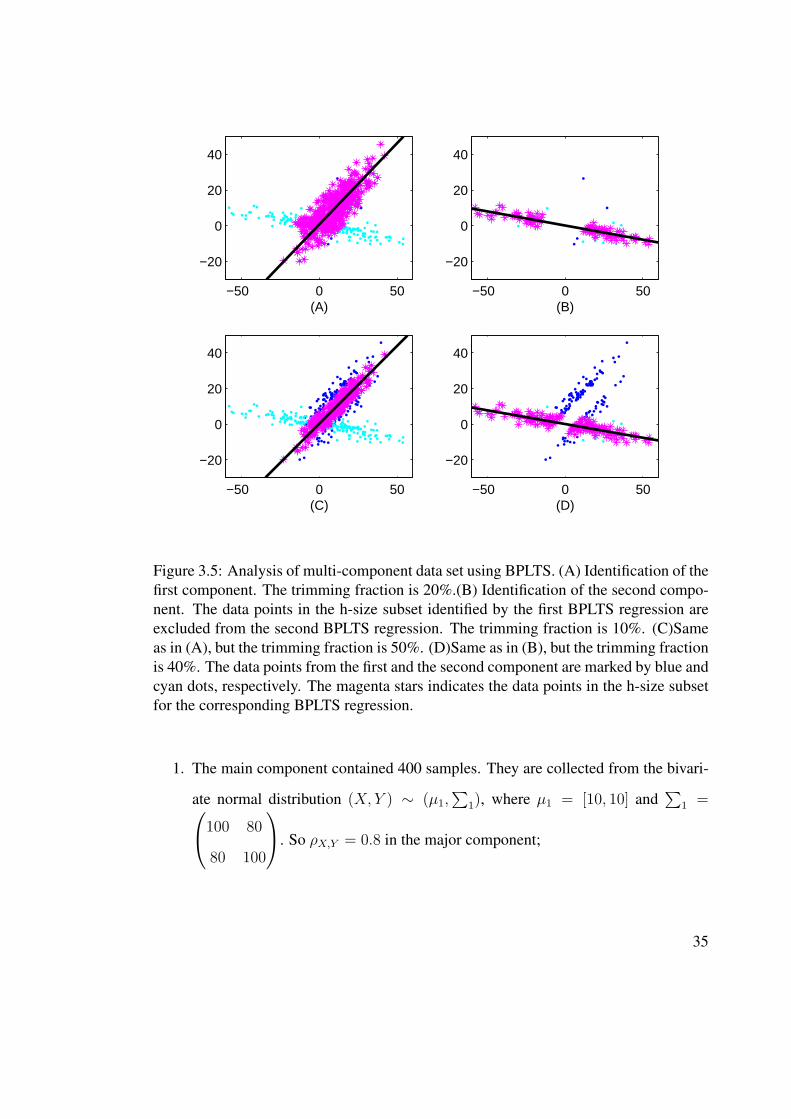
Figure 3.5: Analysis of multi-component data set using BPLTS. (A) Identification of thefirst component. The trimming fraction is 20%.(B) Identification of the second compo-nent. The data points in the h-size subset identified by the first BPLTS regression areexcluded from the second BPLTS regression. The trimming fraction is 10%. (C)Sameas in (A), but the trimming fraction is 50%. (D)Same as in (B), but the trimming fractionis 40%. The data points from the first and the second component are marked by blue andcyan dots, respectively. The magenta stars indicates the data points in the h-size subsetfor the corresponding BPLTS regression.

1. The main component contained 400 samples. They are collected from the bivari-

ate normal distribution (X,Y ) ∼ (µ1,∑

1), where µ1 = [10, 10] and∑

1 =100 80

80 100

. So ρX,Y = 0.8 in the major component;

35

2. The minor component contained 200 samples. They are collected from the bivari-

ate normal distribution (X,Y ) ∼ (µ2,∑

2), where µ1 = [0, 0] and∑

2 =500 −80

−80 20

. So ρX,Y = −0.8 in the minor component.

As shown in Figure 3.5, the relation between x and y is correctly identified in the

first BPLTS regression(see Figure 3.5A and C). Then the relation between x and y in the

second component is correctly estimated by the second BPLTS regression(see Figure

3.5B and C). The choosing of trimming fraction is whatsoever flexible. The trimming

fractions for the first BPLTS are 20% and 50% in Figure 3.5A and Figure 3.5C respec-

tively, both give the correct estimation. In the second BPLTS regression, a trimming

fraction of either 50% in Figure 3.5B or 40% in Figure 3.5D gives the correct estima-

tion. These results show that BPLTS can be used to analyze those data sets with multiple

components.

3.5 Subset correlation analysis using BPLTS

−40 −20 0 20 40

−50

0

50

100

x

y

r = 0.31sub−r = 0.90

−40 −20 0 20 40

−40

−20

0

20

40

60

y

z

r = 0.27sub−r = 0.88

−40 −20 0 20 40−40

−20

0

20

40

x

z

r = 0.12sub−r = −0.02

Figure 3.6: Subset correlation analysis using BPLTS. (A) 50%-subset correlationbetween x and y. (B) 50%-subset correlation between y and z. (C) 50%-subset cor-relation between x and z.

36

In the data set with multiple components, we may not expect the correlation between

two variable across all the data points. For example, two variables x and y may corre-

lated with each other in only one component that represents 50% data points. We can

define P-subset correlation as the correlation of two variables in the subset identified

by BPLTS with trimming fraction 1-P, where 0 < P ≤ 1. For instance, we may have

variables X, Y and Z, where X and Y are correlated in some conditions; Y and Z are cor-

related in some other conditions. Therefore, if we have n observation of (X,Y, Z), we

would expect X and Y are correlated in a subset of data points, Y and Z are correlated

in another subset of data points,but no correlation between X and Z. Using the ordinary

correlation measurement that estimate the liner relationship across all the data points

would fail to identify the underlying relations between them. But subset correlation

works in this situation. To simulate this situation, we perform the following procedures:

1. Generate (Xi, Yi), i = 1...200 from the bivariate normal distribution (X,Y ),

where µ = (20, 20) and Σ =

0.25 0.8

0.8 4

.

2. Generate (Yi, Zi), i = 201...400 from the bivariate normal distribution (Y, Z),

where µ = (−10,−10) and Σ =

4 0.8

0.8 0.25

.

3. Generate Xi, i = 201...400 and Zj, j = 1...200 from uniform distribution

Unif(−40, 40).

Then we obtain the data set in which X and Y are correlated ( PCC = 0.8) in 50% data

points; Y and Z are correlated ( PCC = 0.8) in the other 50% data points.

The result is shown in Figure 3.6, we can find that the ordinary Pearson correlation

coefficients are ρxy = 0.31, ρyz = 0.27, and ρyz = 0.12, respectively. But the 50%

subset Pearson correlation coefficient are ρ50%xy = 0.90, ρ50%

yz = 0.88, and ρ50%yz = −0.02,

37

respectively. This indicates that the subset correlation can correctly expose the linear

relationships among the three variables.

3.6 Scale dependency of BPLTS

1800 2000 2200 2400 2600 2800

2000

3000

4000

5000

(A)1.8 2 2.2 2.4 2.6 2.8

x 104

2000

3000

4000

5000

(B)

1800 2000 2200 2400 2600 2800

2

3

4

5

x 104

(C)1.8 2 2.2 2.4 2.6 2.8

x 104

2

3

4

5

x 104

(D)

y = 1.30x − 482.62 y = 0.086x + 480.68

y = 17x − 13873 y = 1.30x − 4826.2

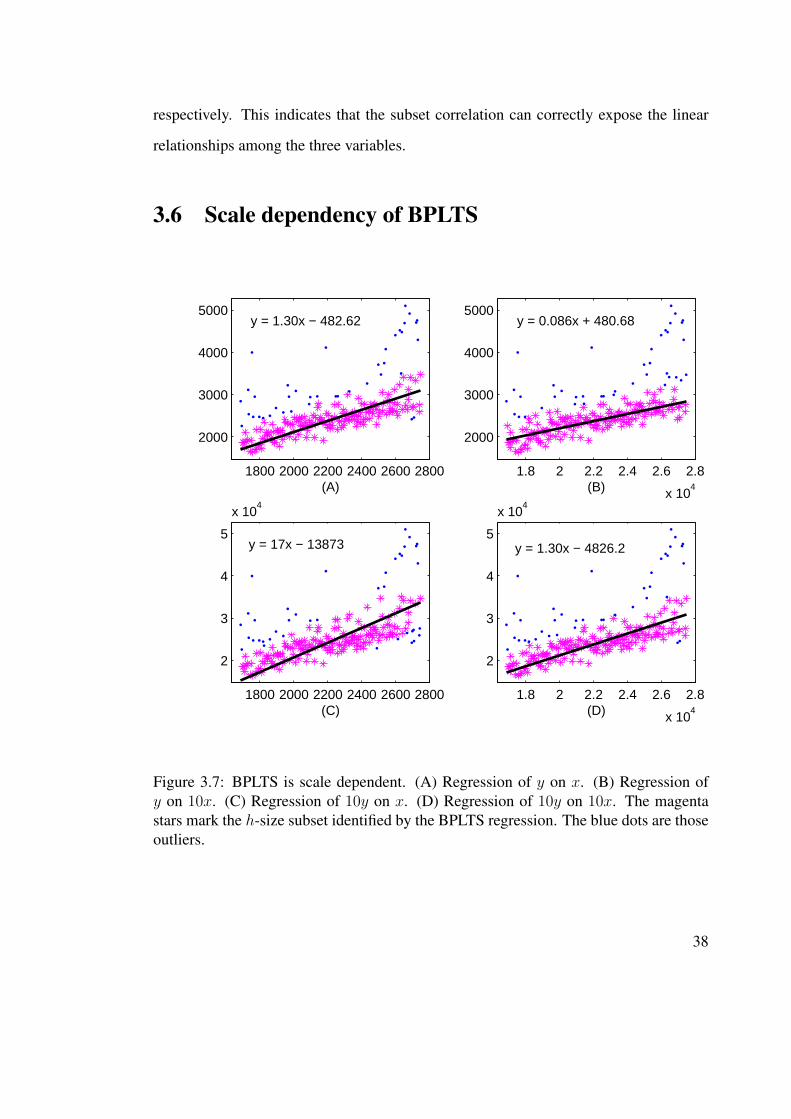
Figure 3.7: BPLTS is scale dependent. (A) Regression of y on x. (B) Regression ofy on 10x. (C) Regression of 10y on x. (D) Regression of 10y on 10x. The magentastars mark the h-size subset identified by the BPLTS regression. The blue dots are thoseoutliers.

38

As we know, the ordinary least trimmed squares (OLTS) is scale equivariant. That

is, it results in the same subset when the scale of x or y is changed. However, the

scale equivariant is not hold by BPLTS regression. As shown in Figure 3.7, the BPLTS

regression gives different h-size subset of data points if we change the scale of y or x.

But if we change the scales of x and y at the same level, BPLTS regression results in the

same h-size subset as the one obtained in the original data.

This bring about the question: what scale should we use for BPLTS regression? For

the observations (xi, yi) of size n, if we have: xi = µxi+ εx and yi = µyi

+ εy, where

εx ∼ N(0, σ2x) and εy ∼ N(0, σ2

y), we should make transformation for either x or y, say

y′ = cy, such that σy′ = σx. After this transformation, the errors from the two variables

are equally considered and thereby the BPLTS regression gives a reasonable results.

39

Chapter 4

Application of BPLTS Method to

Microarray Normalization

Microarray technologies have been widely used in recent years, which provide expres-

sion measurement of tens of thousand genes at the same time. One of the key step for

microarray data analysis is normalization. After normalization, gene expression mea-

surements from various arrays are comparable and can be used to detect gene expression

changes. In this chapter, we will introduce a novel microarray normalization method that

is based on our new developed perpendicular least trimmed squares (BPLTS).

4.1 Introduction to microarray technologies and nor-

malization

Microarray is a key technique in the study of functional genomics. It measures abun-

dance of mRNAs by hybridization to appropriate probes on a glass chip. The current

technique can hold hundreds of thousands of probes on a single chip. This allows us to

have snapshots of expression profiles of a living cell. In the thesis, we mainly consider

high-density oligonucleotide arrays. The Affymetrix GeneChip R© uses 11-20 probe

pairs, which are short oligonucleotides of 25 base pairs, to represent each gene, and as a

whole they are called a probe set [Aff01, LDB+96]. Each probe pair consist of a perfect

match (PM) and a mis-match (MM) probe that differ only in the middle (13-th) base.

40

Mis-match probes are designed to remove the effects of non-specific binding, cross-

hybridization, and electronic noise. Ideally, probes are arranged on a chip in a random

fashion. But in customized arrays, this is not always true.

From microarray measurements, we seek differentiation of mRNA expression

among different cells. However, each array has a “block effect” due to variation in

RNA extraction, labeling, fluorescent detection, etc. Without statistical treatment, this

block effect is confounded with real expression differentiation. The statistical treat-

ment of reducing the block effect is defined to be normalization. It is usually done at

the probe level. Several normalization methods for oligonucleotide arrays have been

proposed and practiced. One approach uses lowess [Cle79] to correct for non-central

and non-linear bias observed in M-A plots [YDLS01]. Another class of approaches

correct for the non-linear bias seen in Q-Q plots [SHG+02, WJJ+02, BIS03]. As dis-

cussed in [ZAZL01, WJJ+02], several assumptions must hold in the methods using

quantiles. First, most genes are not differentially regulated; Second, the number of up-

regulated genes roughly equals the number of down-regulated genes; Third, the above

two assumptions hold across the signal-intensity range.

Our perspective of normalization is that of blind inversion [Li03]. The basic idea is

to find a transformation for the target array so that the joint distribution of hybridization

levels of the target and reference array matches a nominal one. Two different ideas exist

to achieve this goal. First, quantiles allows us to compare distributions and the Q-Q plot

is the standard graphical tool for the purpose. The normalization proposed in [SHG+02,

WJJ+02, BIS03] aims to match the marginal distribution of hybridization levels from

the target with that from reference. Although slight and subtle difference exists between

the two principles, quantile methods work well for arrays with little differentiation. The

second idea is regression, either linear or non-linear [YDLS01, SLSW01].

41

4.2 Application of BPLTS to Microarray normalization

When we compare two arrays in which a substantially large portion of genes are differ-

entially expressed, we need to identify a “base” subset for the purpose of normalization.

This subset should exclude those probes corresponding to differentially expressed genes

and abnormal probes due to experimental variation. A similar concept “invariant set”

is defined in [SLEW, TOR+01, KCM02]. We use perpendicular least trimmed squares

(BPLTS) to identify the base for normalization and to estimate the transformation in a

simultaneous fashion. Substantial differentiation is protected in BPLTS by setting an

appropriate trimming fraction. The exact BPLTS solution is computed by the algorithm

we described in Chapter 2.

Array-specific spatial patterns may exist due to uneven hybridization and measure-

ment process. For example, reagent flow during the washing procedure after hybridiza-

tion may be uneven; scanning may be non-uniform. We have observed different spatial

patterns from one array to anther. To taken this into account, we divide each array into

sub-arrays that consist of a few hundred probes, and normalize probe intensities within

each sub-array.

Statistical principle of normalization Suppose we have two arrays: one reference

and one target. Denote the measured fluorescence intensities from the target and refer-

ence arrays by {Uj, Vj}. Denote true concentrations of specific binding molecules by

(Uj , Vj). Ideally, we expect that (Uj , Vj)=(Uj , Vj). In practice, measurement bias exists

due to uncontrolled factors and we need a normalization procedure to adjust measure-

ment. Next we have another look at normalization. Consider a system with (Uj Vj) as

42

input and (Uj , Vj) as output. Let h = (h1, h2) be the system function that accounts for

all uncontrolled biological and instrumental bias; namely,

Uj = h1(Uj) ,

Vj = h2(Vj) .

The goal is to reconstruct the input variables (Uj , Vj) based on the output variables

(Uj , Vj). It is a blind inversion problem [Li03], in which both input values and the

effective system are unknown. The general idea is to find a transformation that matches

the distributions of input and output. This leads us to the question: what is the joint

distribution of true concentrations (Uj , Vj)? First, let us assume that the target and

reference array are biologically undifferentiated. Then the differences between the target

and reference are purely caused by random variation and uncontrolled factors. In this

ideal case, it is reasonable to assume that the random variables {(Uj, Vj), j = 1, · · · })

are independent samples from a joint distribution Ψ whose density centers around the

straight line U = V , namely, E(V |U) = U . The average deviations from the straight

line measures the accuracy of the experiment. If the effective measurement system h is

not an identity one, then the distribution of the output, denoted by Ψ, could be different

from Ψ. An appropriate estimate h of the transformation should satisfy the following:

the distribution h−1(Ψ) matches Ψ, which centers around the line V = U . In other

words, the right transformation straightens out the distribution of Ψ.

Next we consider the estimation problem. Roughly speaking, only the component of

h1 relative to h2 is estimable. Thus we let v = h2(v) = v. In addition, we assume that

h1 is a monotone function. Denote the inverse of h1 by g, then we expect the following

is valid.

E[V |U ] = U , or E[V |g(U)] = g(U) .

43

Proposition 6. Suppose the above equation is valid. Then g is the minimizer of

minl E(V − l(U))2.

According to the well known fact of conditional expectation, E[V |g(U)] = g(U)

minimizes E[V − l1(g((U))]2 with respect to l1. Next write l1(g(U)) = l(U). This fact

suggests that we estimate g by minimizing∑

j (vj − g(uj))2. When necessary, we can

impose smoothness on g by appropriate parametric or non-parametric forms.

Differentiation fraction and undifferentiated probe set Next we consider a more

complicated situation. Suppose that a proportion λ of all the genes are differentially

expressed while other genes are not except for random fluctuations. Consequently, the

distribution of the input is a mixture of two components. One component consists of

those undifferentiated genes, and its distribution is similar to Ψ. The other component

consists of the differentially expressed genes and is denoted by Γ. Although it is diffi-

cult to know the form of Γ as a priori, its contribution to the input is at most λ. The

distribution of the input variables (Uj , Vj) is the mixture (1 − λ) Ψ + λ Γ. Under the

system function h, Ψ and Γ are transformed respectively into distributions denoted by

Ψ and Γ; That is, Ψ = h(Ψ), Γ = h(Γ). This implies that the distribution of the output

(Uj , Vj) is (1 − λ) Ψ + λ Γ. If we can separate the two components Ψ and Γ, then the

transformation h of some specific form could be estimated from the knowledge of Ψ

and Ψ.

Spatial pattern and sub-arrays Normalization can be carried out in combination

with a stratification strategy. On the high-density oligonucleotide array, tens of thou-

sands of probes are laid out on a chip. To take into account any plausible spatial variation

in h, we divide each chip into sub-arrays, or small squares, and carry out normalization

for probes within each sub-array. To get over any boundary effect, we allow sub-arrays

44

to overlap. A probe in a overlapping regions gets multiple adjusted values from sub-

arrays it belongs to, and we take their average.

In each sub-array contains only a few hundred probes, we choose to parameterize

the function g by a simple linear function α + β u, in which the background α and scale

β represent respectively uncontrolled additive and multiplicative effects. Therefore, we

apply BPLTS method to estimate α and β. Furthermore, by setting a proper trimming

fraction ρ, we expect the corresponding size-h set identified by BPLTS is a subset of

the undifferentiated probes explained earlier. Obviously, the trimming fraction ρ should

be larger than the differentiation fraction λ. We call this BPLTS based normalization

method SUB-SUB normalization. The details of sub-array normalization can be found

in [CL05]

Implementation and SUB-SUB normalization We have developed a module to

implement the normalization method describe above, referred as SUB-SUB normal-

ization. The core code is written in C, and we have an interfaces with Bioconductor in

R. The input of this program is a set of Affymetrix CEL files and output are their CEL

files after normalization. Three parameters need to be specified: sub-array size, over-

lapping size and trimming fraction. The sub-array size specified the size of the sliding

window. The overlapping size controls the smoothness of window-sliding. Trimming

fraction specifies the break down value in LTS. An experiment with an expected higher

differentiation fraction should be normalized with a higher trimming fraction.

4.3 Application of SUB-SUB normalization

Microarray data sets To test the effectiveness of sub-array normalization, we

apply it to two microarray data sets. The first one is Affymetrix Spike-

in data set includes fourteen arrays obtained from Affymetrix HG-U95 chips.

45

Fourteen genes in these arrays are spiked-in at given concentrations in a

cyclic fashion known as a Latin square design. The data are available from

http://www.affymetrix.com/support/technical/sample data/datasets.affx. In the follow-

ing analysis, we chose eight arrays out of the complete data set and split them into two

groups. The first group contains four arrays: 1521m99hpp av06, 1521n99hpp av06,

1521o99hpp av06, 1521p99hpp av06. The second group contains four arrays: 1521-

q99hpp av06, 1521r99hpp av06, 1521s99hpp av06 and 1521t99hpp av06. For conve-

nience, we abbreviate these arrays by M, N, O, P, Q, R, S, T. As a result, the concentra-

tions of thirteen spiked-in genes in the second group are two-fold lower. The concen-

trations of the remaining spike-in gene are respectively 0 and 1024 in the two groups.

In addition, two other genes are so controlled that their concentrations are also two-fold

lower in the second group compared to the first one.

The second data set is also from the same Affymetrix web site, which contains two

technical replicates using yeast array YG-S98. We will use them to study the variation

between array replicates.

Spike-in data Figure 4.1 shows the distribution of log transformed expression levels

of probes and genes in each of the eight arrays before and after SUB-SUB normal-

ization. The expression level for a gene is calculated by combining all the probe lev-

els corresponding to a genes using ”medianpolish” summarization method provided by

Bioconductor. As shown, the expression measurement have various distribution without

normalization, which is result from systematic errors and indicates that normalization is

required for comparison of these arrays. After normalization the distributions of expres-

sion measurement are comparable both in probe level and in gene level. This result show

that SUB-SUB can effectively reduce the systematical errors.

46

56

78

910

11

(A)

56

78

910

11

(B)

67

89

10

(C)

67

89

10

(D)

Figure 4.1: Distribution of log transformed expression measurement. (A) probe levelbefore SUB-SUB normalization. (B)probe level after SUB-SUB normalization. (C)gene level before SUB-SUB normalization. (D)gene level after SUB-SUB normaliza-tion. SUB-SUB parameters: window size 20× 20; overlapping size 10; trimming frac-tion: 80%.

We carry out SUB-SUB normalization to each of the eight arrays using Array M as

the reference. We experimented with different sub-array sizes, overlapping sizes and

trimming fractions. Figure 4.2 shows the M-A plots summarized from the eight arrays

after normalization, namely, the log-ratios of expressions between the two groups versus

the abundance. The sub-array size is 20×20, the overlapping size is 10 and the trimming

factor ranging from 0 to 40% are used. Our result indicates that both the sub-array

47

6 8 10 12 14

−0.

20.

00.

20.

40.

6

6 8 10 12 14

−0.

20.

00.

20.

40.

6

(A)

6 8 10 12 14

−0.

20.

00.

20.

40.

6

6 8 10 12 14

−0.

20.

00.

20.

40.

6

(B)

6 8 10 12 14

−0.

20.

00.

20.

40.

6

6 8 10 12 14

−0.

20.

00.

20.

40.

6

(C)

6 8 10 12 14

−0.

20.

00.

20.

40.

6

6 8 10 12 14

−0.

20.

00.

20.

40.

6

(D)

Figure 4.2: M-A plots of spike-in data after Sub-Sub normalization. The x-axis is theaverage of log-intensities from two arrays. The y-axis is their difference after normal-ization. (A)trimming fraction is 0. (B)trimming fraction is 10%. (C)trimming fractionis 20%. (D)trimming fraction is 40%. The red points represent those Spike-in genes.Window size 20× 20; Overlapping size: 10.

size (data not shown) and trimming fraction matter substantially for normalization. In

other words, stratification by spatial neighborhood and selection of break down value in

BPLTS do contribute a great deal to normalization. When the trimming fraction is set to

zero, BPLTS degenerates into ordinary least squares (OLS). As shown in Figure 4.2A,

the OLS doesn’t make a good normalization. Overlapping size has a little contribution

in this data set.

48

0.0 0.2 0.4 0.6 0.8 1.0

0.0

0.2

0.4

0.6

0.8

1.0

(A)

0.0 0.2 0.4 0.6 0.8 1.0

0.0

0.2

0.4

0.6

0.8

1.0

(B)

(C)

1.0 1.1 1.2 1.3 1.4 1.5 1.6

010

2030

4050

60

(D)

0.8 1.0 1.2 1.4 1.6 1.8

010

2030

4050

6070

Figure 4.3: The slope matrices of two arrays show different spatial patterns in scale.The common reference is Array M. (A) Array P versus M; (B) Array N versus M. Theirhistograms are shown at bottom correspondingly in (C) and (D).

We then investigate the existence of spatial pattern. The HG-U95 chip has 640×640

spots on each array. We divided each array into sub-arrays of size 20×20. We run

simple LTS regression on the target with respect to the reference for each sub-array.

This results in an intercept matrix and a slope matrix of size 32×32, representing the

spatial difference between target and reference in background and scale. We first take

49

Array M as the common reference. In Figure 4.3, the slope matrices of Array P and

M are respectively shown in the subplots at top left and top right, and their histograms

are shown in the subplots at bottom left and bottom right. Two quite different patterns

are observed. Similar phenomenon exists in patterns of α. The key observation is that

spatial patterns are array-specific and unpredictable to a great extent. This justifies the

need of adaptive normalization.

6 8 10 12 14

−2

−1

01

2

6 8 10 12 14

−2

−1

01

2

(A)

6 8 10 12 14

−2

−1

01

2

6 8 10 12 14

−2

−1

01

2

(B)

6 8 10 12 14

−2

−1

01

2

6 8 10 12 14

−2

−1

01

2

(C)

6 8 10 12 14

−2

−1

01

2

6 8 10 12 14

−2

−1

01

2

(D)

Figure 4.4: M-A plots of perturbed spike-in data set after SUB-SUB normalization. Thex-axis is the average of log-intensities from two arrays. The y-axis is their differenceafter normalization. In the top four subplots, 20% randomly selected genes have beenartificially up-regulated by 2.5 fold in Array Q, R, S, and T. The differentiated genes aremarked red, and undifferentiated genes are marked black. The trimming fractions in thesubplots are: (A) 0%; (B) 10%; (C) 30%; (D) 50%.

50

Perturbed Spike-in data SUB-SUB normalization protects substantial differentiation

by selecting an appropriate trimming fraction in LTS. To test this, we generate an arti-

ficial data set with relatively large fraction of differentiation by perturbing the HG-U95

spike-in dataset. Namely, we randomly choose 20% genes and increase their corre-

sponding probe intensities by 2.5 fold in the four arrays in the second group. We then

run SUB-SUB normalization on the perturbed data set with various trimming fractions.

The results are shown in Figure 4.4 for four trimming fractions, 50%, 30%, 10%, and

0%. AS shown, the normalization is satisfactory when the trimming fraction is above

30%, or 10% larger than the nominal differentiation fraction.

6 8 10 12 14

0.00

0.02

0.04

0.06

0.08

0.10

0.12

A

|M|

6 8 10 12 14

0.00

0.02

0.04

0.06

0.08

0.10

0.12

A

|M|

6 8 10 12 14

0.00

0.02

0.04

0.06

0.08

0.10

0.12

A

|M|

6 8 10 12 14

0.00

0.02

0.04

0.06

0.08

0.10

0.12

A

|M|

6 8 10 12 14

0.00

0.02

0.04

0.06

0.08

0.10

0.12

A

|M|

6 8 10 12 14

0.00

0.02

0.04

0.06

0.08

0.10

0.12

A

|M|

6 8 10 12 14

0.00

0.02

0.04

0.06

0.08

0.10

0.12

A

|M|

6 8 10 12 14

0.00

0.02

0.04

0.06

0.08

0.10

0.12

A

|M|

noneloessinvariantsetquantiles

PLTS−10%PLTS−20%PLTS−30%PLTS−40%

Figure 4.5: The lowess curves of |M | versus A values by various normalization methods.

51

Variation reduction by sub-array normalization Stratification is a statistical tech-

nique to reduce variation. Sub-array normalization can be regarded as a way of strat-

ification. We normalize the yeast array 2-121502 versus 2-121501 by various normal-

ization methods available from Bioconductor. Since the two arrays are replicates, the

difference between them is due to experimental variation. In the resulting M-A plots,

we fit lowess [Cle79] curves to the absolute values of M, or |M |. These curves measure

the variation between the two arrays after normalization, see Figure 4.5. The sub-array

normalization achieves the minimal variation. As variation is reduced, signal to noise

ratio is enhanced and power of significance tests is increased. Furthermore, a smaller

trimming fraction in sub-array normalization reduces more variation. This suggests the

following rules to determine trimming fraction for sub-array normalization : (1) One

must select a trimming fraction that is large enough to ensure the robustness of the

BPLTS estimation. (2) If the first rule is satisfied, a smaller trimming fraction is more

efficient in terms of variation reduction.

52

References

[Aff01] Affymetrix Microarray Suite User Guide Santa Clara, CA: Affymetrix. 5thedn. 2001.

[BIS03] B. Bolstad, R. A. Irizarry, and M. Astrand T. P. Speed. A comparison ofnormalization methods for high density oligonucleotide array data based onbias and variance. Bioinformatics, 19:185–193, 2003.

[CL05] C. Cheng and L. M. Li. Sub-array normalization subject to differentiation.Nucleic Acids Research, 37:55655573, 2005.

[Cle79] W. S. Cleveland. Robust locally weighted regression and smoothing scatter-plots. J. Amer. Statist. Assoc., 74:829–836, 1979.

[CR88] R. J. Carroll and D. Ruppert. Transformation and Weighting in Regression.Chapman and Hall, New York, 1988.

[H95] O. Hossjer. Exact computation of the least trimmed squares estimate in sim-ple linear regression. Computational Statistics and Data Analysis, 19:265–282, 1995.

[Haw93] D. M. Hawkins. The feasible set algorithm for least median of squaresregression. Computational Statistics and Data Analysis, 16:81–101, 1993.

[jH73] P. j. Huber. Robust regression: asymptotics, conjectures and monte carlo.Ann. Stat., 1:799–821, 1973.

[KCM02] T. Kepler, L. Crosby, and K. Morgan. Normalization and analysis of DNAmicroarray data by self-consistensy and local regression. Genome Biology,3:1–12, 2002.

[LDB+96] D. J. Lockhart, H. Dong, M. C. Byrne, M. T. Follettie, M. V. Gallo,M. S. Chee M. Mittmann, C. Want, M. Kobayashi, H. Horton, and E. L.Brown. DNA expression monitoring by hybridization of high densityoligonucleotide arrays. Nature Biotechnology, 14:1675–1680, 1996.

53

[LH74] C. L. Lawson and R. J. Hanson. Solving Least Squares Problems. Prentice-Hall, 1974.

[Li03] L. M. Li. Blind inversion needs distribution (BIND): the general notion andcase studies. Science and Statistics: A Festschrift for Terry Speed, 40:273–293, 2003.

[Li05] M. L. Li. An algorithm for computing exact leat-trimmed squares estimateof simple linear regression with constraints. Comutational Statistics andData Analysis, 48:717–734, 2005.

[Lue87] D. G. Luenberger. Linear and Nonlinear Programming. Addison-WesleyPublishing Company, 1987.

[Qua] http://mathworld.wolfram.com/quarticequation.html.

[RD99] P. J. Rousseeuw and K. Van Driessen. Computing LTS Regression for LargeData Sets. Technical Report, University of Antwerp, 1999.

[RL99] P. J. Rousseeuw and A. M. Leroy. Robust Regression and Outlier Detection.John Wiley & Sons, New York, 1999.

[Rou84] P. J. Rousseeuw. Least median squares regression. Journal of AmericanStatistical Association, 88:1279–1281, 1984.

[RY84] P. J. Rousseeuw and V. Yohai. Robust regression by means of S-estimators.Springer Verlag, New York, 1984.

[SHG+02] I. A. Sidorov, D. A. Hosack, D. Gee, J. Yang, M. C. Cam, R. A. Lempicki,and D. S. Dimitrov. Oligonucleotide microarray data distribution and nor-malization. Information Sciences, 146:67–73, 2002.

[SL03] G. A. Seber and A. J. Lee. Linear regression analysis. 2nd edn. A JohnWiley & Sons Publication, New York, 2003.

[SLEW] E. E. Schadt, C. Li, B. Ellis, and W. H. Wong. Feature extraction andnormalization algorithms for high-density oligonucleotide gene expressionarray data. Journal of Cellular Biochemistry, Supplement 37.

[SLSW01] E. E. Schadt, C. Li, C. Su, and W. H. Wong. Analyzing high-densityoligonucleotide gene expression array data. Journal of Cellular Biochem-istry, 80:192–202, 2001.

[SP95] P. B. Stark and R. L. Parker. Bounded-variable least-squares: an algorithmand applications. Computational Statistics, 10:129–141, 1995.

54

[STA01] STATA 7 Reference Manual A-G. STATA Press, College Station, 1995-2001.

[TOR+01] G. C. Tseng, M. Oh, L. Rohlin, J. C. Liao, and W. H. Wong. Issues incDNA microarray analysis: quality filtering,channel normalization, mod-els of variations and assessment of gene effects. Nucleic Acids Research,29:2549–2557, 2001.

[V96] J. A. Vısek. Sensitivity analysis of m-estimates. Ann. Ins. Statist. Math.,48:469–495, 1996.

[V00] J. A. Vısek. On the diversity of estimates. Computational Statistics andData Analysis, 34:67–89, 2000.

[vHL02] S. van Huffel and P. Lemmerling. Total Least Square andErrors-in-Variables Modelling. Kluwer Academic Pulisher, Dor-drecht/Boston/London, 2002.

[VR99] W. N. Venables and B. D. Ripley. Modern Applied Statistics with S-PLUS.4th edn. Springer, New York, 1999.

[WBS99] H. P. William, P. F. Brian, and A. T. Saul. Numerical Recipes in Fortran.2nd edn. Press syndicate of the university of cambridge, 1999.

[Wei] E. W. Weisstein. http://mathworld.wolfram.com/leastsquaresfittingperpendicularoffsets.html.

[WJJ+02] C. Workman, J. Jensen, H. Jarmer, R. BerkaAND L. Gautier, B. Nielsen,H. Saxild, C. Nielson, S. Brunak, and S. Knudsen. A new nonlinear nor-malization method for reducing variability in DNA microarray experiments.Genome Biology, 3:1–16, 2002.

[YDLS01] Y. H. Yang, S. Dudoit, P. Luu, and T. P. Speed. Normalization for cDNAmicroarray data. Microarrays: Optical Technologies and Informatics, 4266,2001.

[Yoh87] V. J. Yohai. High breakdown point and high efficiency robust estimates forregression. Annals of Statistics, 1:253–270, 1987.

[ZAZL01] A. Zien, T. Aigner, R. Zimmer, and T. Lengauer. Centralization: a newmethod for the normalization of gene expression data. Bioinformatics,17:323–331, 2001.

55