Symbolic Integration - University of Iowahomepage.divms.uiowa.edu/~stroyan/CTLC3rdEd/3... · Symbolic Integration ... to trying to use the rules of diﬀerentiation in reverse. You

Chapter 13

Symbolic Integration

This chapter contains the basic tricks of the “symbolic integration” trade. The goal of this chapteris not to make you a slow innacurate integration software, but rather to help you understand thebasics well enough to use modern integration software effectively.

The basic methods of integration are important, but there are many more tricks that areuseful in special situations. The computer knows most of the special tricks but sometimes a basicpreliminary hand computation allows the computer to calculate a very complicated integral that itcannot otherwise do. A change of variables often clarifies the meaning of an integral. Integrationby parts is theoretically important in both math and physics.

We will encounter a few of the special tricks later when they arise in important contexts. Thecable of a suspension bridge can be described by a differential equation, which can be antidifferen-tiated with the “hyperbolic cosine.” If you decide to work on that project, you will want to learnthat trick. “Partial fractions” is another integration trick that arises in the logistic growth model,the S-I-S disease model, and the linear air resistance model in a basic form. We will take thatmethod up when we need it.

The Fundamental Theorem of Integral Calculus 12.13 gives us an indirect way to exactly com-pute the limit of approximations by sums of the form

f [a]∆x+ f [a+∆x]∆x+ f [a+ 2∆x]∆x+ · · ·+ f [b−∆x]∆x =b−∆xXx=a

step ∆x

[f [x]∆x]

We have Z b

af [x] dx = lim

∆x→0

b−∆xXx=a

step ∆x

[f [x]∆x] ≈b−δxXx=astep δx

[f [x] δx]

but the limit can be computed without forming the sum. The Fundamental Theorem says:If we can find F [x] so that dF [x] = f [x] dx, for all a ≤ x ≤ b, thenZ b

af [x] dx = lim

∆x→0

b−∆xXx=a

step ∆x

[f [x]∆x] = F [b]− F [a]

Finding an “antiderivative” lets us skip from the left side of the above equations to the right sidewithout going through the limit in the middle.

This indirect computation of the integral works any time we can find a trick to figure out anantiderivative. There are many such tricks, or “techniques,” and the computer knows them all.Your main task in this chapter is to understand the fundamental techniques and their limitations,rather than to develop skill at very elaborate integral computations.

308

Chapter 13 - SYMBOLIC INTEGRATION 309

The rules of integration are more difficult than the rules of differentiation because they amountto trying to use the rules of differentiation in reverse. You must learn all the basic techniques tounderstand this, but we will not wallow very deep into the swamp of esoteric techniques. That isleft for the computer.

13.1 Indefinite Integrals

The first half of the Fundamental Theorem means that we can often find an integral in two steps:1) Find an antiderivative, 2) compute the difference in values of the antiderivative. It makes nodifference which antiderivative we use. We formalize notation that breaks up these two steps.

One antiderivative of 3x2 is x3, since dx3

dx = 3x2, but another antiderivative of 3x2 is x3 + 273,

since the derivative of the constant 273 (or any other constant) is zero. The integralR ba 3x

2dx maybe computed with either antiderivative.Z b

a3x2dx = x3|ba = b3 − a3

= [x3 + 273]|ba = [b3 + 273]− [a3 + 273] = b3 − a3

Our next result is the converse of the result that says the derivative of a constant is zero. Itsays that if the derivative is zero, the function must be constant. This is geometrically obvious -draw the graph of a function with a zero derivative!

Theorem 13.1 The Zero-Derivative TheoremSuppose F [x] and G [x] are both antiderivatives for the same function f [x] on the interval [a, b];that is, dF

dx [x] =dGdx [x] = f [x] for all x in [a, b]. Then F [x] and G [x] differ by a constant for all x

in [a, b].

Proof:The function H [x] = F [x]−G [x] has zero derivative on [a, b]. We have

H [X]−H [a] =

Z X

a0 dx = 0

by the first half of the Fundamental Theorem and direct computation of the integral of zero.If X is any real value in [a, b], H [X] −H [a] = 0. This means H [X] = H [a], a constant. In

turn, this tells us that F [X]−G [X] = F [a]−G [a], a constant for all X in [a, b].


Definition 13.1 Notation for the Indefinite IntegralThe indefinite integral of a function f [x] denotedZ

f [x] dx

is equal to the collection of all functions F [x] with differential

dF [x] = f [x] dx

or derivative dFdx [x] = f [x].

We write “+c” after an answer to indicate all possible antiderivatives. For example,ZCos[θ] dθ = Sin[θ] + c

Exercise Set 13.1 Verify that both x2 and x2 + π equalR2x dx.


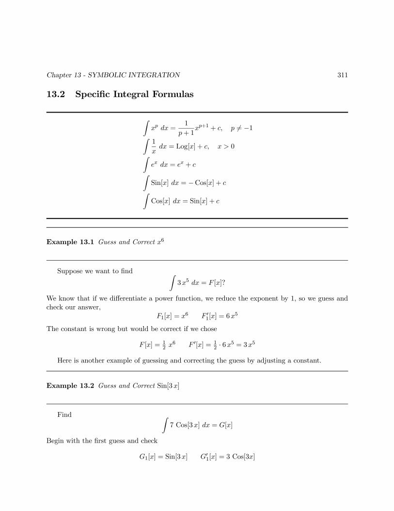
13.2 Specific Integral Formulas

Zxp dx =

1

p+ 1xp+1 + c, p 6= −1Z

1

xdx = Log[x] + c, x > 0Z

ex dx = ex + cZSin[x] dx = −Cos[x] + cZCos[x] dx = Sin[x] + c

Example 13.1 Guess and Correct x6

Suppose we want to find Z3x5 dx = F [x]?

We know that if we differentiate a power function, we reduce the exponent by 1, so we guess andcheck our answer,

F1[x] = x6 F 01[x] = 6x5

The constant is wrong but would be correct if we chose

F [x] = 12 x6 F 0[x] = 1

2 · 6x5 = 3x5

Here is another example of guessing and correcting the guess by adjusting a constant.

Example 13.2 Guess and Correct Sin[3x]

Find Z7 Cos[3x] dx = G[x]

Begin with the first guess and check

G1[x] = Sin[3x] G01[x] = 3 Cos[3x]


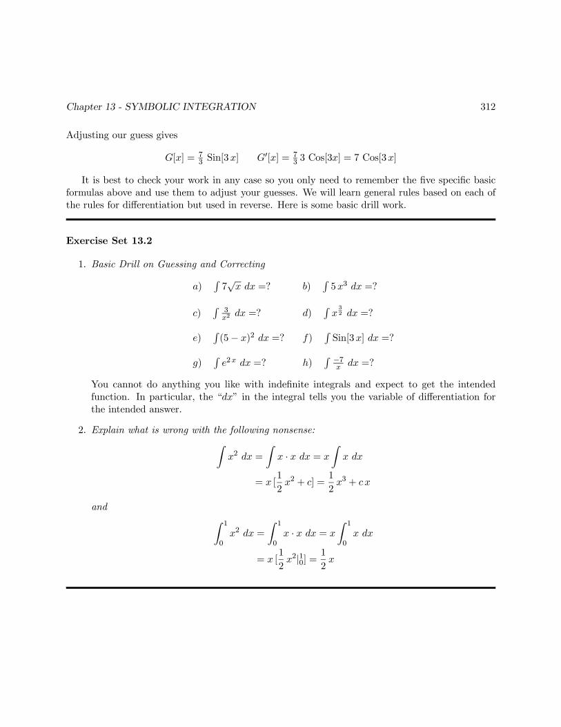
Adjusting our guess gives

G[x] = 73 Sin[3x] G0[x] = 7

3 3 Cos[3x] = 7 Cos[3x]

It is best to check your work in any case so you only need to remember the five specific basicformulas above and use them to adjust your guesses. We will learn general rules based on each ofthe rules for differentiation but used in reverse. Here is some basic drill work.

Exercise Set 13.2

1. Basic Drill on Guessing and Correcting

a)R7√x dx =? b)

R5x3 dx =?

c)R

3x2

dx =? d)Rx32 dx =?

e)R(5− x)2 dx =? f)

RSin[3x] dx =?

g)Re2x dx =? h)

R −7x dx =?

You cannot do anything you like with indefinite integrals and expect to get the intendedfunction. In particular, the “dx” in the integral tells you the variable of differentiation forthe intended answer.

2. Explain what is wrong with the following nonsense:Zx2 dx =

Zx · x dx = x

Zx dx

= x [1

2x2 + c] =

1

2x3 + c x

and Z 1

0x2 dx =

Z 1

0x · x dx = x

Z 1

0x dx

= x [1

2x2|10] =

1

2x


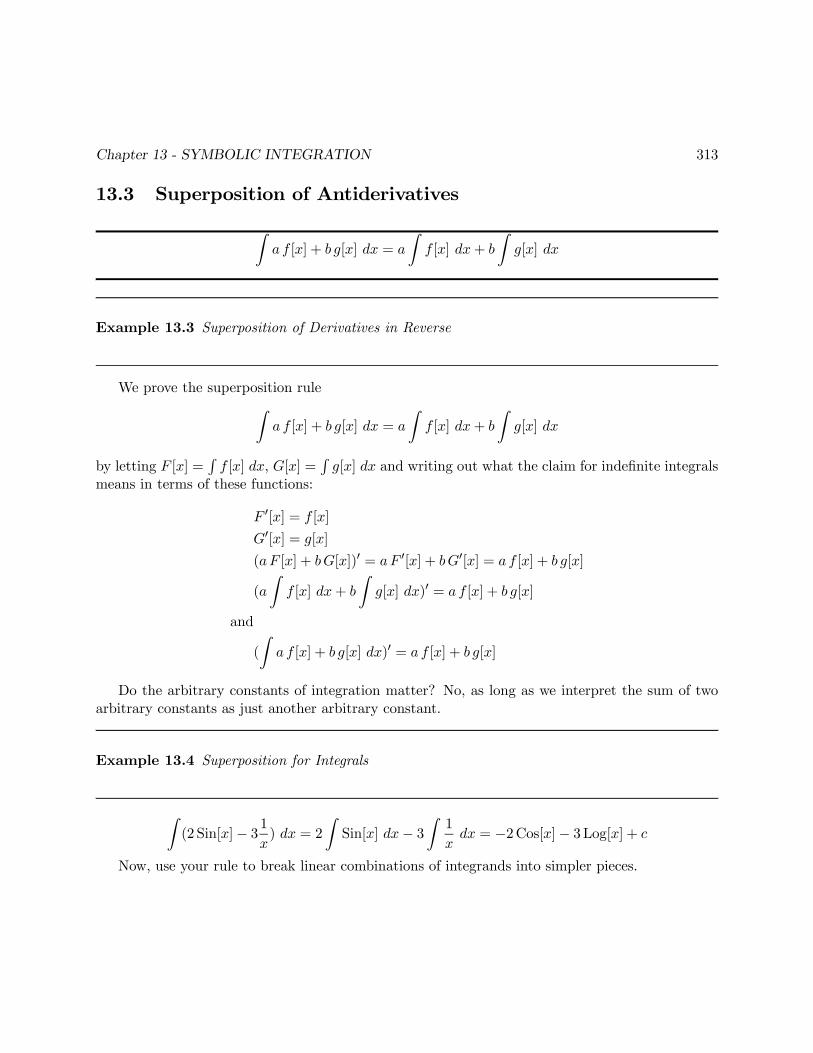
13.3 Superposition of Antiderivatives

Za f [x] + b g[x] dx = a

Zf [x] dx+ b

Zg[x] dx

Example 13.3 Superposition of Derivatives in Reverse

We prove the superposition ruleZa f [x] + b g[x] dx = a

Zf [x] dx+ b

Zg[x] dx

by letting F [x] =Rf [x] dx, G[x] =

Rg[x] dx and writing out what the claim for indefinite integrals

means in terms of these functions:

F 0[x] = f [x]

G0[x] = g[x]

(aF [x] + bG[x])0 = aF 0[x] + bG0[x] = a f [x] + b g[x]

(a

Zf [x] dx+ b

Zg[x] dx)0 = a f [x] + b g[x]

and

(

Za f [x] + b g[x] dx)0 = a f [x] + b g[x]

Do the arbitrary constants of integration matter? No, as long as we interpret the sum of twoarbitrary constants as just another arbitrary constant.

Example 13.4 Superposition for Integrals

Z(2 Sin[x]− 31

x) dx = 2

ZSin[x] dx− 3

Z1

xdx = −2Cos[x]− 3Log[x] + c

Now, use your rule to break linear combinations of integrands into simpler pieces.


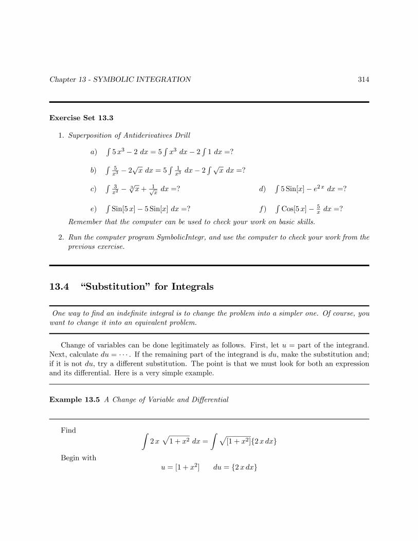
Exercise Set 13.3

1. Superposition of Antiderivatives Drill

a)R5x3 − 2 dx = 5 R x3 dx− 2 R 1 dx =?

b)R

5x3− 2√x dx = 5

R1x3

dx− 2 R √x dx =?

c)R

3x2 − 3

√x+ 1√

xdx =? d)

R5 Sin[x]− e2x dx =?

e)RSin[5x]− 5 Sin[x] dx =? f)

RCos[5x]− 5

x dx =?

Remember that the computer can be used to check your work on basic skills.

2. Run the computer program SymbolicIntegr, and use the computer to check your work from theprevious exercise.

13.4 “Substitution” for Integrals

One way to find an indefinite integral is to change the problem into a simpler one. Of course, youwant to change it into an equivalent problem.

Change of variables can be done legitimately as follows. First, let u = part of the integrand.Next, calculate du = · · · . If the remaining part of the integrand is du, make the substitution and;if it is not du, try a different substitution. The point is that we must look for both an expressionand its differential. Here is a very simple example.

Example 13.5 A Change of Variable and Differential

Find Z2x

p1 + x2 dx =

Z p[1 + x2]{2xdx}

Begin withu = [1 + x2] du = {2xdx}


We replace the expression for u and du, thereby obtaining the simpler problem: FindZ p[u] {du} =

Zu12 du

=1

1 + 12

u1+12 + c

=2

3u32 + c

The expression 23 u

32 +c is not an acceptable answer to the question, “What functions of x have

derivative 2x√1 + x2?” However, if we remember that u = 1 + x2, we can express the answer as

2

3u32 + c =

2

3[1 + x2]

32 + c

Checking the answer will show why this method works. We use the Chain Rule:

y = 23 u

32 u = 1 + x2

sodydu =

2332 u

32−1 du

dx = 2x

and

dy

dx=

dy

du

du

dx= u

12 2x = 2x

p1 + x2

or

dy = 2xp1 + x2 dx

Example 13.6 Another Change

You must substitute for the differential du associated with your change of variables u = · · · .Sometimes this is a little complicated. For example, suppose we try to computeZ

2xp1 + x2 dx

with the change of variable and differential

v =√1 + x2 dv = x√

1+x2dx

Our integral becomes Z2v[ rest of above]


with the rest of the above equal to xdx. We can find dv = x√1+x2

dx by multiplying numerator and

denominator by√1 + x2, so our integral becomesZ2p1 + x2 x

√1 + x2√1 + x2

dx =

Z2³p

1 + x2´2[

x√1 + x2

dx]

= 2

Zv2dv =

2

3v3 + c

=2

3

£1 + x2

¤ 32

This is the same answer as before, but the substitution was more difficult on the dv piece.

Example 13.7 A Failed Attempt

Sometimes an attempt to simplify an integrand by change of variables will lead you to eithera more complicated integral or a situation in which you cannot make the substitution for thedifferential. In these cases, scratch off your work and try another change.

Suppose we try a grand simplification ofZ2x

p1 + x2 dx

taking

w = xp1 + x2 dw =

µp1 + x2 +

x2√1 + x2

¶dx

We might substitute w for the whole integrand, but there is nothing left to substitute for dw andwe cannot complete the substitution. We simply have to try a different method.

Example 13.8 A Less Obvious Substitution with u =√x

We may be slipping into the symbol swamp, but a little wallowing can be fun. Here is a change


of variable and differential with a twist:Z √x

1 + xdx

u =√x ⇔ u2 = x (x > 0)

du =1

2√xdx ⇔ 2u du = dxZ

u

1 + u22 u du = 2

Zu2

1 + u2du = 2

·Z µ1−

µ1

1 + u2

¶¶du

¸= 2

Zdu− 2

Z1

1 + u2du = 2u− 2 ArcTan[u] + cZ √

x

1 + xdx = 2

√x− 2 ArcTan[√x] + c

Now, you try it.

Exercise Set 13.4

Change of Variable and Differential Drill

a)R

1(3x−2)2 dx =? b)

R2t√1−t2 dt =?

c)Rx(3 + 7x2)3 dx =? d)

R 3y(2+2y2)2

dy =?

e)R(Cos[x])3 Sin[x] dx =? f)

R Cos[Log[x]]x dx =?

g)ReCos[θ] Sin[θ] dθ =? h)

RSin[a x+ b] dx =?

If you have checked several indefinite integration problems that you computed with a change ofvariable and differential, you probably realize that the Chain Rule lies behind the method. Perhapsyou can formalize your idea.

Problem 13.1 The Chain Rule in ReverseUse the Chain Rule for differentiation to prove the indefinite integral form of “Integration by

Substitution.” Once you have this indefinite rule, use the Fundamental Theorem to prove the definiterule.


13.5 Change of Limits of Integration

When we want an antiderivative such asR2x√1 + x2 dx, we have no choice but to re-substitute

the expressions for new variables back into our answer. In the first example of the previous section,Z2xp1 + x2 dx =

2

3u32 + c =

2

3[1 + x2]

32

However, when we want to compute a definite integral such asZ 7

52xp1 + x2 dx

we can change the limits of integration along with the change of variables. For example,

u = 1 + x2 du = 2x dx

u[5] = 26 u[7] = 50

so the new problem is to find Z 50

26u12 du

which equals2

3u32 |5026 =

2

3[50

32 − 26 32 ] ≈ 235.702− 88.383 = 147.319

We recommend that you do your definite integral changes of variable this way:

Procedure 13.1 To compute Z b

af [x] dx

1. Set a portion of your integrand f [x] equal to a new variable u = u[x].

2. Calculate du =?? dx.

3. Calculate u[a] = α and u[b] = β.

4. Substitute both the function and the differential in f [x] dx for g[u] du.

5. Compute

Z β

αg[u] du


Pay Me Now or Pay Me Later:You can compute the antiderivative in terms of x and then use the original limits of integration,

but there is a danger that you will lose track of the variable with which you started. If you arecareful, both methods give the same answer; for example,Z 7

52xp1 + x2 dx =

2

3[1 + x2]

32 |75 =

2

3

³[1 + 72]

32 − [1 + 52] 32

´≈ 147.319

Exercise Set 13.5

1. Change of Variables with Limits Drill

a)R 10

x1+x2

dx =? b)R π/60 Sin[3θ] dθ =?

c)R 32

2x(x2−3)2 dx =? d)

R 10 ax+ b dx =?

e)R 10

3x2−11+√x−x3 dx = 0 because of the new limits.

f)R 10 x e

−x2 dx =? g)R π/20 Cos[θ] Sin[θ] dθ =?

2. Use the change of variable u =√x and associated change of differential to convertR √

x Cos[√x] dx into a multiple of

Ru2 Cos[u] du.

13.5.1 Integration with Parameters

Change of variables can make integrals with parameters, which are important in many scientific andmathematical problems, into specific integrals. For example, suppose that ω and a are constant.Then Z

Sin[ω t] dt

u = ω t

du = ω dt ⇔ 1

ωdu = dtZ

Sin[ω t] dt =

ZSin[u]

1

ωdu =

1

ω

ZSin[u] du


and Z1

a2 + x2dt =

Z1

a2(1 + (x/a)2)dx =

1

a2

Z1

1 + (x/a)2dx

u =x

a

du =1

adx ⇔ a du = dxZ

1

a2 + x2dt =

1

a2

Z1

1 + u2a du =

1

a

Z1

1 + u2du

This type of change of variable and differential may be the most important kind for you tothink about because the computer can give you specific integrals, but you may want to see how anintegral depends on a parameter.

Problem 13.2 Pull the Parameter OutShow that Z 3

0

p9− x2 dx = 3

Z 3

0

p1− (x/3)2 dx = 9

Z 1

0

p1− u2 du

Show that the area of a circle of radius r is r2 times the area of the unit circle. First, changevariables to obtain the integrals below and then read on to interpret your computation.Z r

0

pr2 − x2 dx = r2

Z 1

0

p1− u2 du

13.6 Trig Substitutions

Study this section if you have a personal need to compute integrals with one of the followingexpressions (and do not have your computer):p

a2 − x2, a2 + x2 orpa2 + x2

You should skim read this section even if you do not wish to develop this skill because thepositive sign needed to go between

(Cos[θ])2 = 1− (Sin[θ])2 and Cos[θ] =p1− (Sin[θ])2

can cause errors in the use of a symbolic integration package. In other words, the computer mayuse the symbolic square root when you intend for it to use the negative.


Example 13.9 A Trigonometric Change of Variables

The following integral comes from computing the area of a circle using the integral. A sinesubstitution makes it one we can antidifferentiate with two tricks from trig.Z 1

0

p1− u2 du =

Z π/2

0

q1− Sin2 [θ] Cos [θ] dθ

because we take the substitution

u = Sin [θ] du = Cos [θ] dθ

u = 0⇔ θ = 0 u = 1⇔ θ = π/2

We know from high school trig that 1 − Sin2 [θ] = Cos2 [θ], so, when the cosine is positive,q1− Sin2 [θ] = Cos [θ] and

Z π/2

0

q1− Sin2 [θ] Cos [θ] dθ =

Z π/2

0Cos2 [θ] dθ

We also know from high school trig (or looking at the graph and thinking a little) that Cos2 [θ] =12 [1 + Cos (2θ)], so Z π/2

0Cos2 [θ] dθ =

1

2[

Z π/2

0dθ +

Z π/2

0Cos (2θ) dθ]

=π

4+1

4

Z π

0Cos [φ] dφ

because we use another change of variables

φ = 2θ dφ = 2dθ

φ = 0⇔ θ = 0 φ = π ⇔ θ = π/2

Finally,1

4

Z π

0Cos [φ] dφ =

1

4[Sin [φ] |π0 ] = 0

as we could have easily seen by sketching a graph of Cos [φ] from 0 to π, with equal areas aboveand below the φ-axis.


Putting all these computations together, we haveZ 1

0

p1− u2 du =

π

4

One explanation why the change of variables in the previous example works is that sine andcosine yield parametric equations for the unit circle. More technically speaking, the (PythagoreanTheorem) identity

(Sin[θ])2 + (Cos[θ])2 = 1 ⇔ (Cos[θ])2 = 1− (Sin[θ])2

becomes the identity (Cos[θ])2 = 1 − u2 when we let u = Sin[θ]. There is an important algebraicdetail when we write

Cos[θ] =p1− (Sin[θ])2

This is false when cosine is negative. For the definite integral above, we wanted 0 ≤ u ≤ 1 andchose 0 ≤ θ ≤ π/2 to put Sin[θ] in this range. It is also true that Cos[θ] ≥ 0 for this range of θ, sothat

Cos[θ] =p1− u2

If the cosine were not positive in the range of interest, the integration would not be valid. More in-formation on this difficulty is contained in the Mathematical Background Chapter on DifferentiationDrill.

An expression such as√a2 − x2 can first be reduced to a multiple of

√1− u2 by taking u = x/a

and writing√a2 − x2 = a

p1− (x/a)2. This means that the expression √a2 − x2 can be converted

to Cos[θ] with the substitutions u = (x/a)2 and u = Sin[θ] (provided cosine is positive on theinterval).

Notice that the substitution u = Cos[θ] converts√1− u2 into

p1− (Cos[θ])2 = Sin[θ], provided

sine is positive. Also note that sine is positive over a different range of angles than cosine.Another trig identity says

(Tan[θ])2 + 1 = (Sec[θ])2 ⇔µSin[θ]

Cos[θ]

¶2+

µCos[θ]

Cos[θ]

¶2=

µ1

Cos[θ]

¶2⇔ (Sin[θ])2 + (Cos[θ])2 = 1

If we make a change of variable u = Tan[θ], then u2 + 1 becomes (Sec[θ])2 and√1 + u2 = Sec[θ]

provided secant is positive.

Example 13.10 The Sine Substitution Without Endpoints

The “cost” of not changing limits of integration in Example 13.9 is the following: The sametricks as above for indefinite integrals yieldZ p

1− u2 du =1

2θ +

1

4Sin[φ]


where u = Sin[θ] and φ = 2 θ. If we really want the antiderivative of√1− u2, then we must express

all this in terms of u.The first term is easy, we just use the inverse trig function

u = Sin[θ] ⇔ θ = ArcSin[u]

The term Sin[φ] = Sin[2 θ] must first be written in terms of functions of θ, (recall the additionformula for sine),

Sin[2 θ] = 2 Sin[θ] Cos[θ]

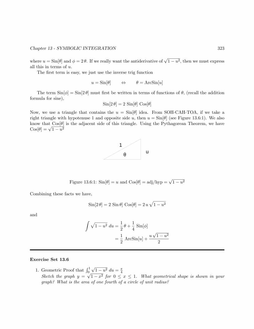
Now, we use a triangle that contains the u = Sin[θ] idea. From SOH-CAH-TOA, if we take aright triangle with hypotenuse 1 and opposite side u, then u = Sin[θ] (see Figure 13.6:1). We alsoknow that Cos[θ] is the adjacent side of this triangle. Using the Pythagorean Theorem, we haveCos[θ] =

√1− u2

1

uθ

1

Figure 13.6:1: Sin[θ] = u and Cos[θ] = adj/hyp =√1− u2

Combining these facts we have,

Sin[2 θ] = 2 Sin θ] Cos[θ] = 2up1− u2

and Z p1− u2 du =

1

2θ +

1

4Sin[φ]

=1

2ArcSin[u] +

u√1− u2

2

Exercise Set 13.6

1. Geometric Proof thatR 10

√1− u2 du = π

4

Sketch the graph y =√1− x2 for 0 ≤ x ≤ 1. What geometrical shape is shown in your

graph? What is the area of one fourth of a circle of unit radius?


2. Compute the integralR 90

√9− x2 dx. (Check your symbolic computation geometrically).

Use the change of variable x = Sin[θ] with an appropriate differential to show thatZ v

0

1√1− x2

dx =

Zdθ = θ... = ArcSin[v]

How large can we take v?

Use the change of variable x = Tan[θ] with an appropriate differential to show thatZ v

0

1

1 + x2dx =

Zdθ = θ... = ArcTan[v]

How large can we take v?

3. Working Back from Trig SubstitutionsSuppose we make the change of variable u = Sin[θ] (as in the integration above). ExpressTan[θ] in terms of u by using Figure 13.6:1 and TOA.

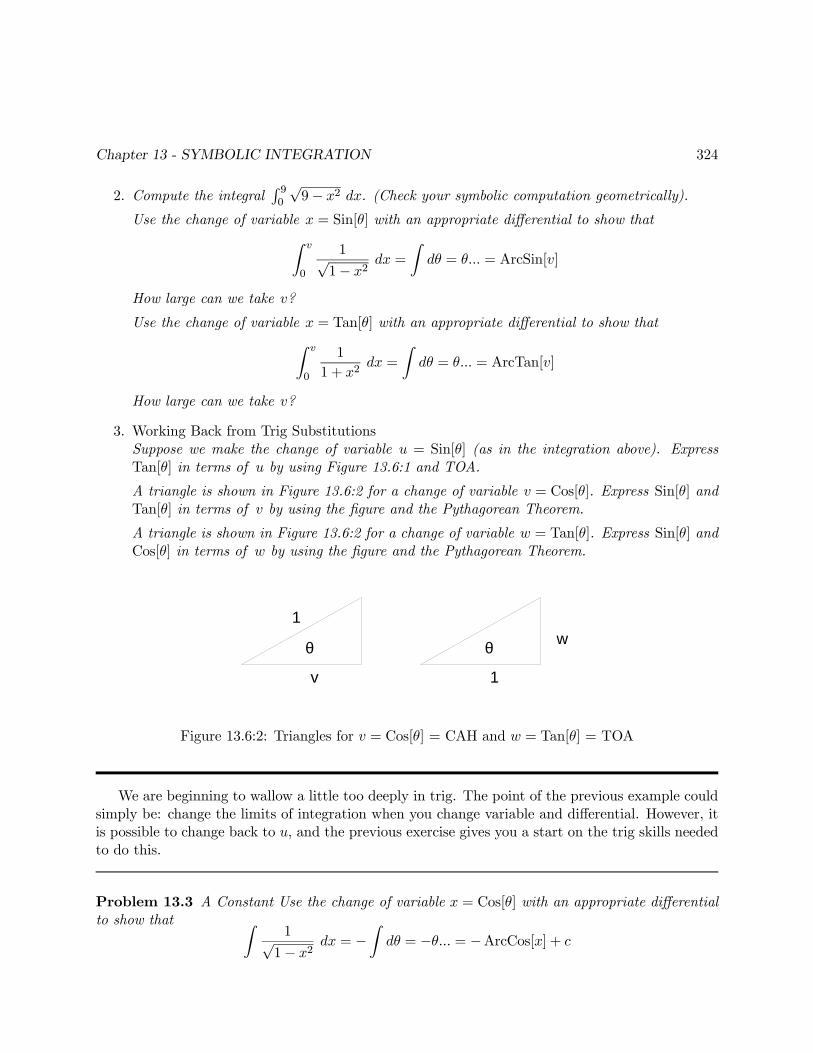
A triangle is shown in Figure 13.6:2 for a change of variable v = Cos[θ]. Express Sin[θ] andTan[θ] in terms of v by using the figure and the Pythagorean Theorem.

A triangle is shown in Figure 13.6:2 for a change of variable w = Tan[θ]. Express Sin[θ] andCos[θ] in terms of w by using the figure and the Pythagorean Theorem.

v

uθ

1

1

wθ

Figure 13.6:2: Triangles for v = Cos[θ] = CAH and w = Tan[θ] = TOA

We are beginning to wallow a little too deeply in trig. The point of the previous example couldsimply be: change the limits of integration when you change variable and differential. However, itis possible to change back to u, and the previous exercise gives you a start on the trig skills neededto do this.

Problem 13.3 A Constant Use the change of variable x = Cos[θ] with an appropriate differentialto show that Z

1√1− x2

dx = −Z

dθ = −θ... = −ArcCos[x] + c


Also, use the change of variable x = Sin[θ] with an appropriate differential to show thatZ1√1− x2

dx =

Zdθ = θ... = ArcSin[x] + c

Is ArcCos[x] = −ArcSin[x]? Ask the computer to Plot ArcSin[x] and −ArcCos[x]. Why dothey look alike? How do they differ? Do the graphs of −Cos[θ] and Sin[θ] look alike? How do theydiffer?

13.7 Integration by Parts

Integration by Parts is important theoretically, but it appears to be just another trick. It is morethan that, but first you should learn the trick.

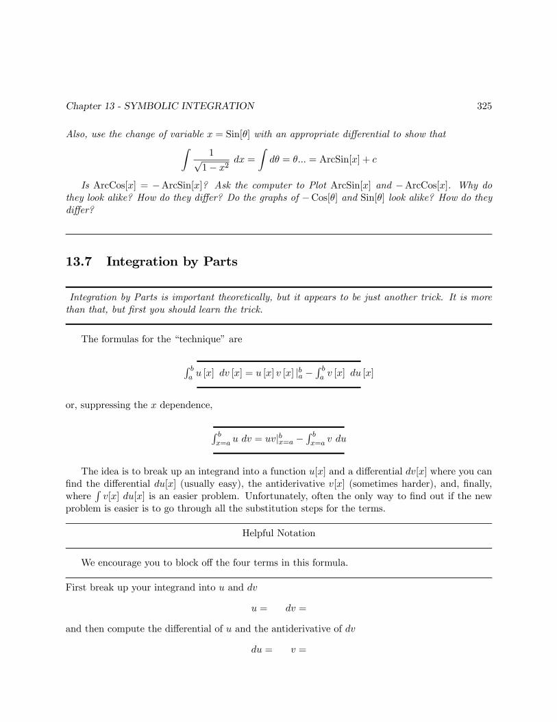
The formulas for the “technique” are

R ba u [x] dv [x] = u [x] v [x] |ba −

R ba v [x] du [x]

or, suppressing the x dependence,

R bx=a u dv = uv|bx=a −

R bx=a v du

The idea is to break up an integrand into a function u[x] and a differential dv[x] where you canfind the differential du[x] (usually easy), the antiderivative v[x] (sometimes harder), and, finally,where

Rv[x] du[x] is an easier problem. Unfortunately, often the only way to find out if the new

problem is easier is to go through all the substitution steps for the terms.

Helpful Notation

We encourage you to block off the four terms in this formula.

First break up your integrand into u and dv

u = dv =

and then compute the differential of u and the antiderivative of dv

du = v =


Here is an example of the use of Integration by Parts.

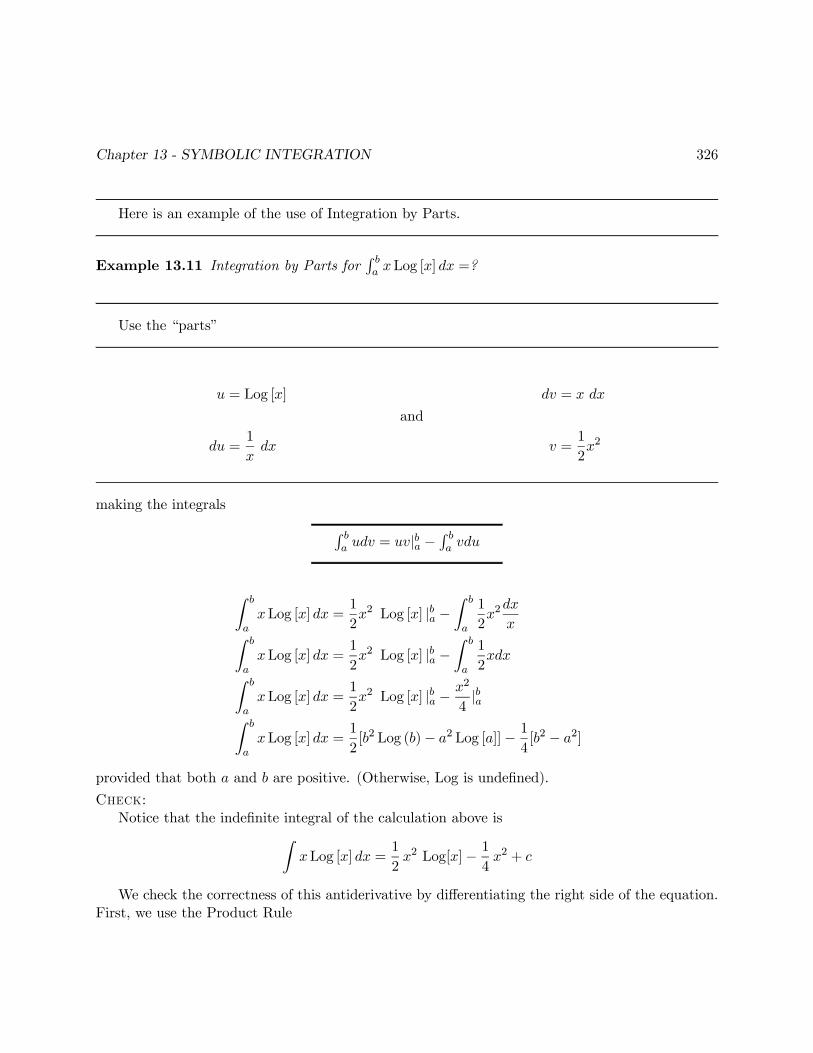
Example 13.11 Integration by Parts forR ba xLog [x] dx =?

Use the “parts”

u = Log [x] dv = x dx

and

du =1

xdx v =

1

2x2

making the integrals R ba udv = uv|ba −

R ba vdu

Z b

axLog [x] dx =

1

2x2 Log [x] |ba −

Z b

a

1

2x2

dx

xZ b

axLog [x] dx =

1

2x2 Log [x] |ba −

Z b

a

1

2xdxZ b

axLog [x] dx =

1

2x2 Log [x] |ba −

x2

4|baZ b

axLog [x] dx =

1

2[b2 Log (b)− a2 Log [a]]− 1

4[b2 − a2]

provided that both a and b are positive. (Otherwise, Log is undefined).

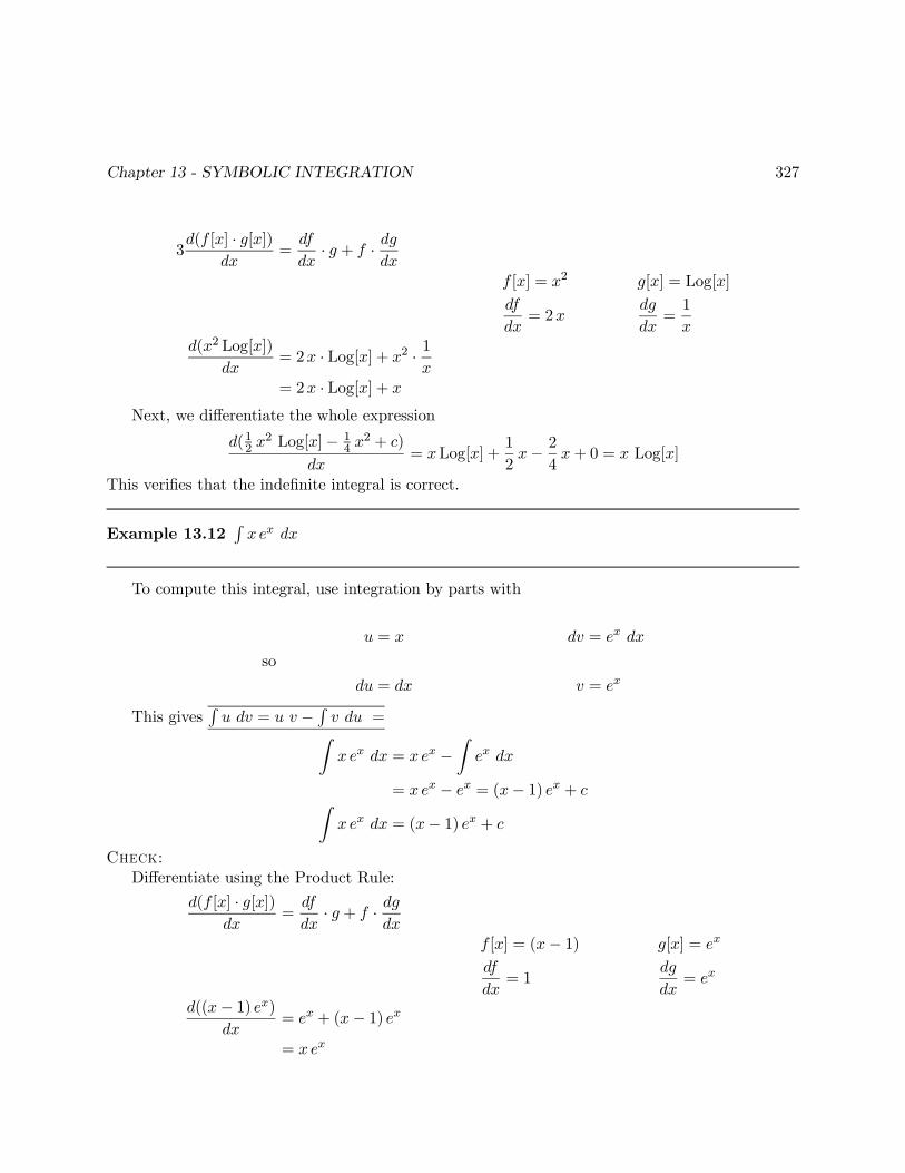
Check:Notice that the indefinite integral of the calculation above isZ

xLog [x] dx =1

2x2 Log[x]− 1

4x2 + c

We check the correctness of this antiderivative by differentiating the right side of the equation.First, we use the Product Rule


3d(f [x] · g[x])

dx=

df

dx· g + f · dg

dxf [x] = x2 g[x] = Log[x]

df

dx= 2x

dg

dx=1

xd(x2 Log[x])

dx= 2x · Log[x] + x2 · 1

x= 2x · Log[x] + x

Next, we differentiate the whole expression

d(12 x2 Log[x]− 1

4 x2 + c)

dx= xLog[x] +

1

2x− 2

4x+ 0 = x Log[x]

This verifies that the indefinite integral is correct.

Example 13.12Rx ex dx

To compute this integral, use integration by parts with

u = x dv = ex dx

so

du = dx v = ex

This givesRu dv = u v − R v du =Z

x ex dx = x ex −Z

ex dx

= x ex − ex = (x− 1) ex + cZx ex dx = (x− 1) ex + c

Check:Differentiate using the Product Rule:

d(f [x] · g[x])dx

=df

dx· g + f · dg

dxf [x] = (x− 1) g[x] = ex

df

dx= 1

dg

dx= ex

d((x− 1) ex)dx

= ex + (x− 1) ex

= x ex


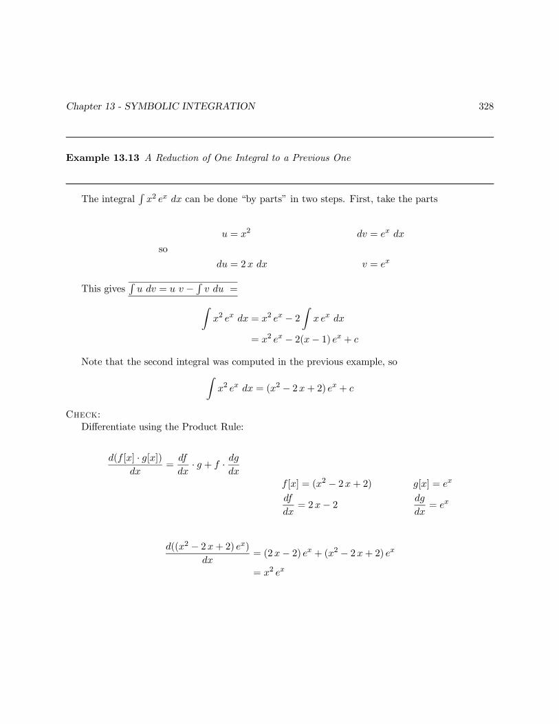
Example 13.13 A Reduction of One Integral to a Previous One

The integralRx2 ex dx can be done “by parts” in two steps. First, take the parts

u = x2 dv = ex dx

so

du = 2x dx v = ex

This givesRu dv = u v − R v du =Z

x2 ex dx = x2 ex − 2Z

x ex dx

= x2 ex − 2(x− 1) ex + c

Note that the second integral was computed in the previous example, soZx2 ex dx = (x2 − 2x+ 2) ex + c

Check:Differentiate using the Product Rule:

d(f [x] · g[x])dx

=df

dx· g + f · dg

dxf [x] = (x2 − 2x+ 2) g[x] = ex

df

dx= 2x− 2 dg

dx= ex

d((x2 − 2x+ 2) ex)dx

= (2x− 2) ex + (x2 − 2x+ 2) ex

= x2 ex


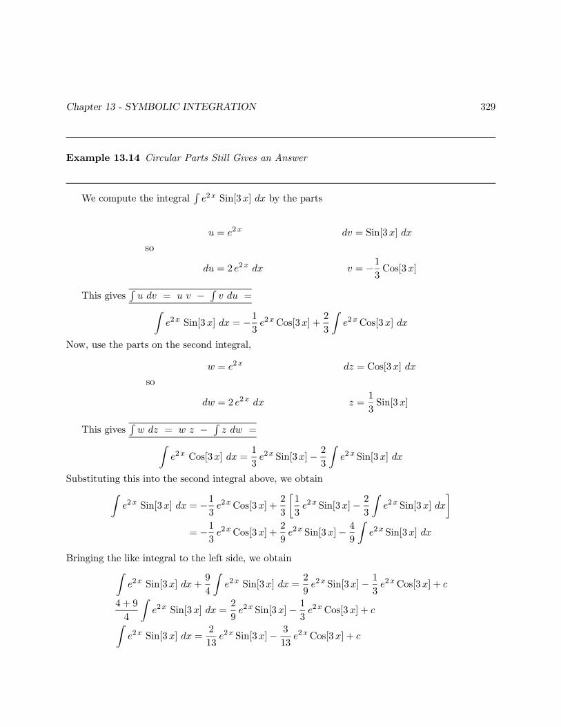
Example 13.14 Circular Parts Still Gives an Answer

We compute the integralRe2x Sin[3x] dx by the parts

u = e2x dv = Sin[3x] dx

so

du = 2 e2x dx v = −13Cos[3x]

This givesRu dv = u v − R

v du =Ze2x Sin[3x] dx = −1

3e2xCos[3x] +

2

3

Ze2xCos[3x] dx

Now, use the parts on the second integral,

w = e2x dz = Cos[3x] dx

so

dw = 2 e2x dx z =1

3Sin[3x]

This givesRw dz = w z − R

z dw =Ze2x Cos[3x] dx =

1

3e2x Sin[3x]− 2

3

Ze2x Sin[3x] dx

Substituting this into the second integral above, we obtainZe2x Sin[3x] dx = −1

3e2xCos[3x] +

2

3

·1

3e2x Sin[3x]− 2

3

Ze2x Sin[3x] dx

¸= −1

3e2xCos[3x] +

2

9e2x Sin[3x]− 4

9

Ze2x Sin[3x] dx

Bringing the like integral to the left side, we obtainZe2x Sin[3x] dx+

9

4

Ze2x Sin[3x] dx =

2

9e2x Sin[3x]− 1

3e2xCos[3x] + c

4 + 9

4

Ze2x Sin[3x] dx =

2

9e2x Sin[3x]− 1

3e2xCos[3x] + cZ

e2x Sin[3x] dx =2

13e2x Sin[3x]− 3

13e2xCos[3x] + c


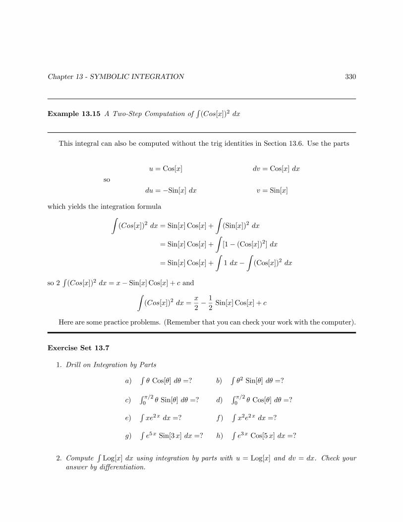
Example 13.15 A Two-Step Computation ofR(Cos[x])2 dx

This integral can also be computed without the trig identities in Section 13.6. Use the parts

u = Cos[x] dv = Cos[x] dx

so

du = −Sin[x] dx v = Sin[x]

which yields the integration formulaZ(Cos[x])2 dx = Sin[x] Cos[x] +

Z(Sin[x])2 dx

= Sin[x] Cos[x] +

Z[1− (Cos[x])2] dx

= Sin[x] Cos[x] +

Z1 dx−

Z(Cos[x])2 dx

so 2R(Cos[x])2 dx = x− Sin[x] Cos[x] + c andZ

(Cos[x])2 dx =x

2− 12Sin[x] Cos[x] + c

Here are some practice problems. (Remember that you can check your work with the computer).

Exercise Set 13.7

1. Drill on Integration by Parts

a)Rθ Cos[θ] dθ =? b)

Rθ2 Sin[θ] dθ =?

c)R π/20 θ Sin[θ] dθ =? d)

R π/20 θ Cos[θ] dθ =?

e)Rxe2x dx =? f)

Rx2e2x dx =?

g)Re5x Sin[3x] dx =? h)

Re3x Cos[5x] dx =?

2. ComputeRLog[x] dx using integration by parts with u = Log[x] and dv = dx. Check your

answer by differentiation.


3. Check the previous indefinite integral from Example 13.14 by using the Product Rule to dif-ferentiate 2

13 e2x Sin[3x]− 3

13 e2xCos[3x].

Compute the integralRe2x Sin[3x] dx by the parts

u = Sin[3x] dv = e2x dx

so

du = 3 Cos[3x] dx v =1

2e2x

4. CalculateR(Sin[x])2 dx.

There is something indefinite about these integrals.

5. What is wrong with the equationZdx

x=

Zx

x2dx = −1 +

Zdx

x

when you use integration by parts with u = x, dv = dxx2 , du = dx, and v = −1

x ? SubtractingRdxx from both sides of the equations above yields

0 = −1

The proof of the Integration by Parts formula is actually easy.

6. The Product Rule in ReverseUse the Product Rule for differentiation to prove the indefinite integral form of Integration byParts. Notice that if H[x] is any function,

RdH[x] = H[x] + c, by definition. Let H = u v

and show that dH = u dv + v du. Indefinitely integrate both sides of the dH equation,

u · v = H[x] =

ZdH =

Zudv +

Zv du

Once you have this indefinite rule, use the Fundamental Theorem to prove the definite rule.

Here are some tougher problems in which you need to use more than one method at a time.

7. (a)RxCos[x] Sin[x] dx =?

Notice thatR(Cos[θ])2 dθ is done above two ways.

(b)Rθ (Cos[θ])2 dθ = ?

Use integrals from the previous drill problems.

(c)R

x3√x2−1 dx =?

HINT: Use parts u = x2 and dv = x dx√x2−1 and compute the dv integral.


(d)R

1x3

q1x − 1 dx = ?

Use parts u = 1x and dv = 1

x2

q1x − 1. Compute the dv integral.

(e)R 10 ArcTan[x] dx = ?Use parts u = ArcTan[x] and dv = dx.

(f)R 10 xArcTan[x] dx = ?Use parts and the previous exercise.

(g)R 10 ArcTan[

√x] dx = ?

Use parts u = ArcTan[√x] and change variables in the resulting integral.

(h)R 94 Sin[

√x] dx = ?

Use parts u = Sin[√x] and dv = dx. Then change variables with w =

√x.

(i)R(Log[x])2 dx = ?Use the parts u = Log[x] and dv = Log[x] dx. Calculate the dv integral.

13.8 Impossible Integrals

There are important limitations to symbolic integration that go beyond the practical difficulties oflearning all the tricks. This section explains why.

Integration by parts and the change of variable and differential are important ideas for thetheoretical transformation of integrals. In this chapter, we tried to include just enough drill work foryou to learn the basic methods. Before the practical implementation of general antidifferentiationalgorithms on computers, development of human integration skills was an important part of thetraining of scientists and engineers. Now, the computer can makes this skill easier to master. Theskill has always had limitations.

Early in the days of calculus, it was quite impressive that integration could be used to learnmany many new formulas such as the classical formulas for the area of a circle or volume of asphere. We saw how easy it was to generalize the integration approach to the volume of a cone.However, some simple-looking integrals have no antiderivative what so ever. This is not the resultof peculiar mathematical examples.

The arclength of an ellipse just means the length measured as you travel along an ellipse.Problem 14.2 asks you to find integral formulas for this arclength. Early developers of calculusmust have tried very hard to compute those integrals with symbolic antiderivatives, but after


more than a century of trying, Liouville proved that there is no analytical expression for thatantiderivative in terms of the classical functions.

The fact that the antiderivative has no expression in terms of old functions does not mean thatthe integral does not exist. If you find the following integral with the computer, you will see apeculiar result: Z

Cos[x2] dx

The innocent-looking integralRCos[x2] dx is not innocent at all. The function Cos[x2] is perfectly

smooth and well behaved, but it does not have an antiderivative that can be expressed in terms ofknown functions. The bottom line is this: Integrals are used to define and numerically computeimportant new functions in science and mathematics, even when they do not have expressions interms of elementary functions. Functions given by integral formulas can still be differentiated justas you did in Exercise 12.8.1.

Exercise Set 13.8

Run the SymbolicIntegr program.

Documents

Symbolic Integration - University of Iowahomepage.divms.uiowa.edu/~stroyan/CTLC3rdEd/3... · Symbolic Integration ... to trying to use the rules of diﬀerentiation in reverse. You