Embed Size (px)
Citation preview

Symbolic Causation Entropy
Carlo Cafaro1, Dane Taylor2, Jie Sun1, and Erik Bollt1
Clarkson University1, Potsdam NY, USA
University of North Carolina2, Chapel Hill NC, USA
cidnet14, Max-Planck Institute, Dresden, Germany

Preliminary thanks
2
1. Claudia Poenisch (…organization/accomodation…)
2. CIDNET14 Coordinators (…present…)
3. Max-Planck Institute, Dresden (…host…)
…my first ten monthsdealing with causality and
networks…
CIDNET14: Causality, Information Transfer and Dynamical Networks
2. 16 → 1.23 → 1.14 → out!

Problem, relevance, and our approach
• What is the problem?
• Why is it relevant?
• Why is it challenging?
• What is our approach? …applications…
(…and, linking dynamical systems theory to information theory via
symbolic dynamics)
3

Part 1: Problem, relevance, challenges
4

The problem in a cartoon
Cause-effect relationships in a soccer game 5
Problem: Infer the coupling structure (cause-effect relationships) of complex systems from time-series data
Causality is the relation
between two events (the
cause and the effect),
where the second event is
understood as a
consequence of the first.
What is causality?

6
Causality
Quiz
• Mario and Pascal
are causally
disconnected
• Mario and Pascal
are negatively
correlated

7
Example:
Remark: CORRELATION ≠ CAUSATION
Summercausal⇒ Drowning
Summercausal⇒ Ice-cream consumption
Ice-cream consumptioncorrelated
↔ Drowning
Ice-cream consumptioncausal? Drowning
correlation does not imply causality

Relevance of the problem
8
Major goals in theoretical physics (science, in general):
• Describe natural phenomena
• Understand, to a certain extent, natural phenomena
…predict the future……reconstruct the past……control phenomena….
…understand what causes what is naturally important…

9
Heart
dynamicsBrain
dynamics
chaoticity &
cardiac rhythmglobal synchronization
& brain activity
…inspired by D.
Chialvo (June19,
cidnet14)
Angelo
Mosso

Challenge: a good solution
• Gather a sufficient amount of relevant data (experimental work)
• Uncover a good causal inference measure (theoretical work)
• Provide an accurate (and, possibly, fast) estimate of such a measure (numerical and computational work)
10
…quoting K. Lehnertz (June 16, cidnet14): …this isa challenge for the next decades to come…

A good causal network inference measure
1. …general applicability and neat interpretation...
2. …immune to false positives and false negatives…
3. …accurate and fast numerical estimation…
Condition (1) →…linear and nonlinear interactions…
Condition (2) →…correct identification of direct couplings in complexsystems with more than two components…
Condition (3) →…appropriate statistical estimation techniques…
11
A. Kraskov, H. Stogbauer, and P. Grassberger, Phys. Rev. E69, 066138 (2004)
J. Runge, J. Heitzig, V. Petoukhov, and J. Kurths, Phys. Rev. Lett. 108, 2587701 (2012)

Some preliminaries(information-theoretic approach to cauality inference)
12
X is a discrete random variable with probability distribution p(x)
HXdef= −∑
x
px logpx ≥ 0 Shannon Entropy
Interpretation: H(X) is a measure of uncertainty associated with X
0.0 0.2 0.4 0.6 0.8 1.00.0
0.2
0.4
0.6
0.8
1.0
p
H(p)
Xdef=
1, with probability p
0, with probability 1 − p
Hp = −p log2p − 1 − p log
21 − p
Example
Hp = bits

13
H X, Ydef= −∑
x, y
p x, y logp x, y
HX|Ydef= −∑
x, y
p x, y logpx|y
M X, Ydef= HX − HX|Y = M Y, X
joint entropy
conditional entropy
mutual information
Interpretation: M(X, Y) is the reduction in uncertainty of X due to the knowledge of Y
M X, Y|Zdef= HX|Z − H X Y, Z
Interpretation: M(X, Y|Z) is the reduction in uncertainty of X due to the knowledge of
Y when Z is given
conditional mutual information
14
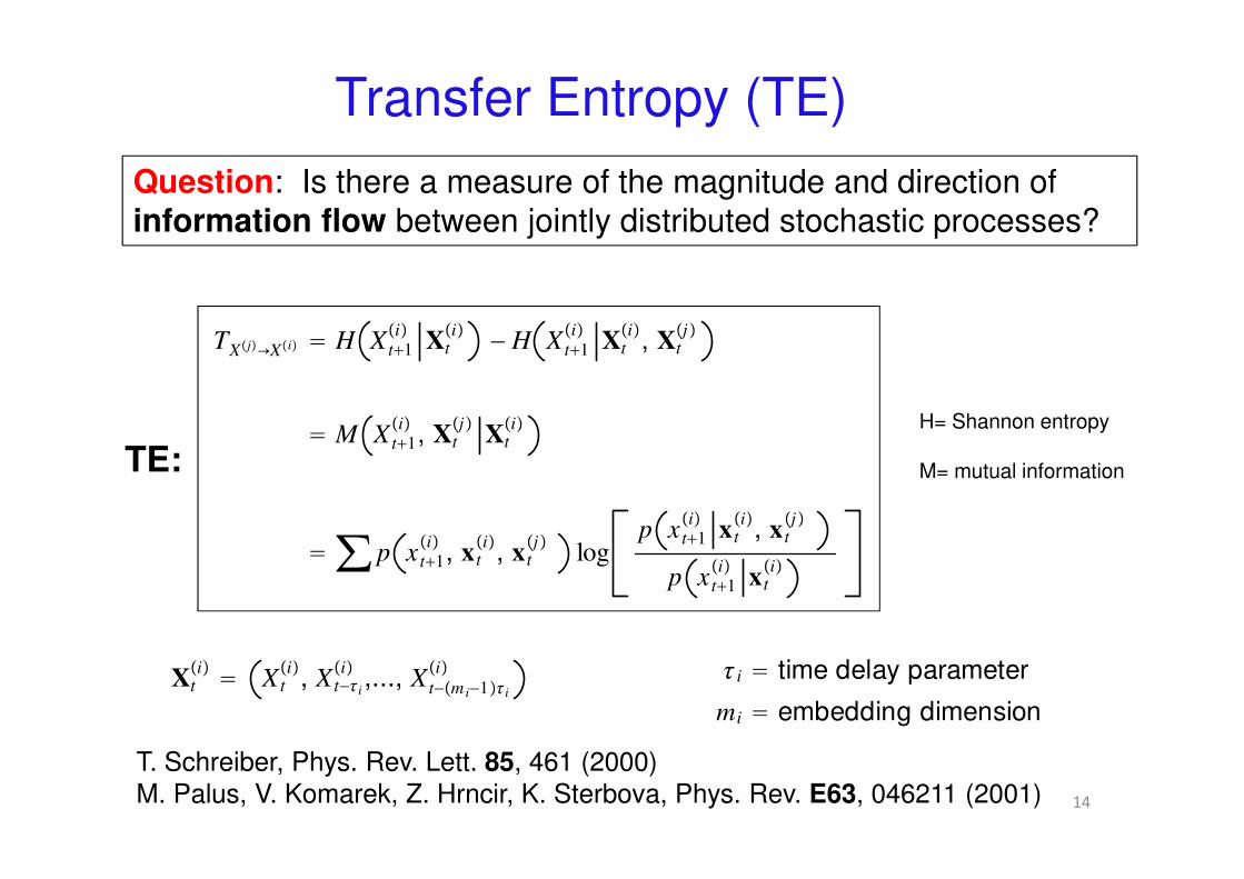
Transfer Entropy (TE)
TXj→Xi = H X t+1i
Xti − H X t+1
iXt
i, Xt
j
= M X t+1i
, Xtj
Xti
= ∑ p x t+1i
, xti
, xtj
logp x t+1
ix ti
, x tj
p x t+1i
xti
TE:
H= Shannon entropy
M= mutual information
Question: Is there a measure of the magnitude and direction of
information flow between jointly distributed stochastic processes?
T. Schreiber, Phys. Rev. Lett. 85, 461 (2000)
M. Palus, V. Komarek, Z. Hrncir, K. Sterbova, Phys. Rev. E63, 046211 (2001)
Xti
= X ti
, X t−τi
i,..., X t−m i−1τi
i τi = time delay parameter
mi = embedding dimension

15
XiXj
Transfer Entropy is a pairwise (asymmetric) measure of information flow

16
T1→2 ≠ T2→1
T1→2 measures the degree of dependence of 2 on 1 (and NOT viceversa)...
Example

Indirect and direct influences
Fact: If a causal interaction is given by 1→2→3, a bivariate analysis
would give a significant link between 1 and 3 that is detected as
being only indirect in a multivariate analysis including 2.
17
true coupling structure
wrong coupling structure
Example
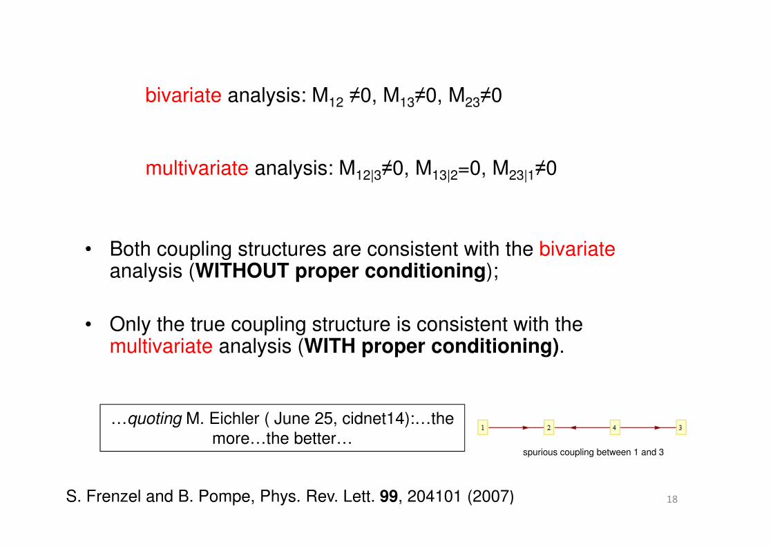
bivariate analysis: M12 ≠0, M13≠0, M23≠0
multivariate analysis: M12|3≠0, M13|2=0, M23|1≠0
• Both coupling structures are consistent with the bivariateanalysis (WITHOUT proper conditioning);
• Only the true coupling structure is consistent with the multivariate analysis (WITH proper conditioning).
18S. Frenzel and B. Pompe, Phys. Rev. Lett. 99, 204101 (2007)
spurious coupling between 1 and 3
…quoting M. Eichler ( June 25, cidnet14):…the
more…the better…

Some (incomplete) history
19
• …quantifying information transfer…
T. Schreiber, Phys. Rev. Lett. 85, 461 (2000) (MPI, Dresden)
M. Palus et al., Phys. Rev. E63, 046211 (2001)
• …bivariate Gaussian processes and TE…
A. Kaiser and T. Schreiber, Physica D166, 43 (2002) (MPI, Dresden)
• …multivariate Gaussian processes and conditional TE…
L. Barnett et al., Phys. Rev. Lett. 103, 238701 (2009)
• …existence and strength of causal relationsips…
J. Runge et al., Phys. Rev. E86, 061121 (2012)

Summary: Part 1 (problem, relevance, challenges)
20
Interplay among:
• Experimentalists (…experimental design…)
• Computational Scientists
(…numerical/computational estimation methods…)
• Theorists (…universal causal inference measure…)
Question: …in the meantime, inspired also by TE, what are we actuallydoing…?

Part 2: Our approach
(the oCSE approach = the optimal Causation Entropy approach)
21

The goal
22
Identify the coupling structure in complex systems
described by dynamical networks
• causal network topology (existence)
• link weights (strength)
• functional dependence between nodes
(…hard problem…)

Some notations
23
complex systems ↔ networks
networks ↔ nodes, links
nodes ↔ dynamical systems
links ↔ interactions
Remark:
Probabilistic approach: dynamical systems modeled in termsof stationary stochastic processes
n = total number of nodes
X t = X t1
,..., X tn
|K | = cardinality of a subset of nodes
X tK
= X t1
,..., X t|K | , with |K | ≤ n

Markovian causal inference framework
24
i : pX t |X t−1, X t−2,... = pX t |X t−1 = pX t ′ |X t ′−1, ∀t, t′;
ii : pX tj
|X t−1 = pX tj
|X t−1
N j, ∀j;
iii : pX tj
|X t−1K ≠ pX t
j|X t−1
L, whenever K ∩ N j ≠ L ∩ N j.
Working hypotheses: (stationary) stochastic processessatisfying the following (Markov) conditions
Main point: for each component j there is a unique (and minimal) set of components Nj that renders the rest of the system irrelevant in makinginferences about X(j)

Causation Entropy (CSE)
J. Sun and E. M. Bollt, Physica D267, 49 (2014) 25
CXJ→XI XK = H X t+1I
XtK − H X t+1
IXt
K, Xt
J
= M X t+1I
, XtJ
XtK
= ∑ p x t+1I
, xtJ
, x tK
logp x t+1
IxtJ
, xtK
p x t+1I
xtK
CSE:
τk r = time delay parameter
mk r = embedding dimension
XtK
= Xtk 1 ,..., Xt
k |K |
1 ≤ r ≤ |K| : Xtk r = X t
k r , X t−1k r ,..., X
t−τkr−1mkr
k r

26
For J = j and K = I = i : CXj→Xi Xi = TXj→Xi
Interpretation: Uncertainty reduction of the future states of
X(I) as a result of knowing the past states of X(J) given that
the past of X(K) is already known.
CSE as a generalization of TE: TXj→Xi → CXJ→XI XK

CSE, uncoditional TE, conditional TE
27
TY−→X+ ≡ CY−→X+|X−
def= HX+ |X− − H X+ Y−, X−
if Y− = X− : TX−→X+ = 0
CY−→X+|Z−
def= HX+|Z− − H X+ Y−, Z−
if Z− = , and Y− = X− : CX−→X+ = HX+ − HX+|X−
CSE and unconditional TE
self-causality cannot be investigated with TE
self-causality can be investigated with CSE
N. J. Cowan et al., PlosOne 7, 1 (2012) networks control & self-causality

28
CSE and conditional TE
X tk def
= X t, X t−1,..., X t−k+1
TY→X|Z
def= H X t+1 X t
k , Z t
m − H X t+1 X tk
, Z tm
, Ytl
CY→X|W
def= HX t+1|W t − H X t+1 W t, Yt
l
if W t = X tk
, Z tm, CY→X|W = TY→X|Z if W t ≠ X t
k , Z t
m, CY→X|W ≠ TY→X|Z
conditional TE
CSE
conditional TE is a special case of CSERemark:
Notation:

The optimal Causation Entropy approach
Goal: For any node-i, find Ni (maximization of CSE)
29
i = node of the graph
Ni = set of nodes that are directly causally connected to node-i
Algorithm 1: Aggregative Discovery
For any node-i, it finds the set of nodes that are
causally connected to node-i (including indirect
and spurious causal connections)
Algorithm 2: Progressive RemovalFor any node-i, it removes indirect and
spurious causal connections
J. Sun, D. Taylor, and E. M. Bollt, arXiv:cs.IT/1401.7574 (2014)

Algorithm 1: Aggregative Discovery
30
Output: For any node-i, it finds Midef= k1,..., k j
Mi contains all types of causal links: direct, indirect, spurious
k1 : 0 < Ck 1→i is max
k2 : 0 < Ck 2→i|k 1 is max
⋮kj : 0 < C
k j→i k 1,..., k j−1is max
kj+1 : Ck j+1→i k 1,..., k j
equals zero ⇒ stop!
Example:

Algorithm 2: Progressive Removal
31
Output: For any node-i, it finds Nidef= direct causal links to node-i
kr with 1 ≤ r ≤ j is removed from Mi when Ck r→i|Mi\k r = 0
Example:
k1 :
Ck 1→i|Mi\k 1 > 0 ⇒ keep k1
Ck1→i|Mi\k 1 = 0 ⇒ remove k1
Suppose we remove k1. Then, Mi → M i′ def= Mi\k1
k2 :
Ck 2→i Mi′\k 2 > 0 ⇒ keep k2
Ck2→i Mi′\k 2 = 0 ⇒ remove k2
⋮Finally, after considering all kr with 1 ≤ r ≤ j, the set Mi becomes Ni
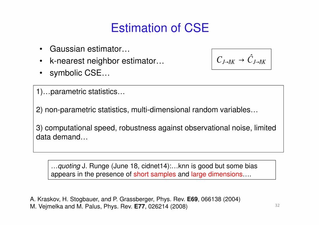
Estimation of CSE
• Gaussian estimator…
• k-nearest neighbor estimator…
• symbolic CSE…
32
CJ→I|K → ĈJ→I|K
1)…parametric statistics…
2) non-parametric statistics, multi-dimensional random variables…
3) computational speed, robustness against observational noise, limiteddata demand…
A. Kraskov, H. Stogbauer, and P. Grassberger, Phys. Rev. E69, 066138 (2004)
M. Vejmelka and M. Palus, Phys. Rev. E77, 026214 (2008)
…quoting J. Runge (June 18, cidnet14):…knn is good but some bias
appears in the presence of short samples and large dimensions….
33
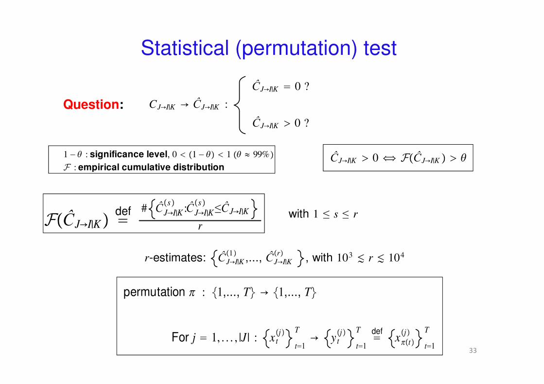
Question:
ĈJ→I|K > 0 FĈJ→I|K > θ
r-estimates: ĈJ→I|K
1,..., ĈJ→I|K
r, with 103 ≲ r ≲ 104
CJ→I|K → ĈJ→I|K :
ĈJ→I|K = 0 ?
ĈJ→I|K > 0 ?
FĈJ→I|Kdef=
# ĈJ→I|K
s:ĈJ→I|K
s ≤ĈJ→I|K
rwith 1 ≤ s ≤ r
permutation π : 1,..., T → 1,..., T
For j = 1, . . . , |J | : x tj
t=1
T→ y t
j
t=1
T def= xπt
j
t=1
T
Statistical (permutation) test
1 − θ : significance level, 0 < 1 − θ < 1 θ ≈ 99%F : empirical cumulative distribution

Example: The oCSE approach & the repressilator
dynamical variables:
pi= concentration of the protein
mi= concentration of mRNA
parameters:
β=ratio of the protein decay rate to the mRNA decay rate
n=Hill coefficient
α0=leakiness of the promotor
α+α0=additional rate of transcription of the mRNA in the absence of inhibitor
34
dm i
dt= −mi +
α1+pj
n + α0
dpi
dt= −βp i − mi
i = lacl, tetR, cl, and j = cl, lacl, tetR
J. Sun, C. Cafaro, and E. M. Bollt, Entropy 16, 3416 (2014)
synthetic biological
oscillator network

35
1 → 1, 2 → 2, 3 → 3, 4 → 4, 5 → 5, 6 → 6
1 → 4, 2 → 5, 3 → 6, 4 → 2, 5 → 3, 6 → 1
1 ≡ mlacl, 2 ≡ mtetR, 3 ≡ mcl
4 ≡ placl, 5 ≡ ptetR, 6 ≡ pcl
Theoretical Jacobian matrix at equilibrium: J ij
theor. def=
∗ 0 0 0 0 ∗
0 ∗ 0 ∗ 0 0
0 0 ∗ 0 ∗ 0
∗ 0 0 ∗ 0 0
0 ∗ 0 0 ∗ 0
0 0 ∗ 0 0 ∗
hypothesis: n = 2, α0 = 0, α = 10, β = 102 ⇒equilibrium: xeq. = 2, 2, 2, 2, 2, 2
J ijdef= ∂ jf i
x = fx

Problem statement: The objective of coupling inference is to
identify the location of the nonzero entries of the Jacobian
matrix through time series generated by the system near
equlibrium
36
Given I6×2 ≡ I6 × I6
def= 1,..., 6 × 1,..., 6 :
● False negative: infer nothing when there is something...
● False positive: infer something when there is nothing...
−def=
card i, j ∈ I6×2 : J ij
theor.≠ 0 ∧ J ij
numer.= 0
card i, j ∈ I6×2 : J ij
theor.≠ 0
+def=
card i, j ∈ I6×2 : J ij
theor.= 0 ∧ J ij
numer.≠ 0
card i, j ∈ I6×2 : J ij
theor.= 0
• Aggregative
discovery
• Progressive
removal

37
Some details
● Preliminary steps:
i) The system starts at equilibrium x∗ = xeq.: xx=x
eq.
= 0;
ii) At time t, apply perturbation ξ to the system: x∗ → xt = x∗ + ξt;
iii) At time t + Δt, measure the rate of response η: η =xt+Δt−xt
Δt=
xt+Δt−x∗−ξtΔt
;
Repeat these steps L-times⇒ ξ l l=1L and η l l=1
L ;
● Parameters:
i) L = number of times the perturbation is applied;
ii) Δt−1 = sample frequency;
iii) σ2 = variance of the Gaussian-distributed variable ξ.

38
● Hypotheses:
i) Δt−1 ≫ 1;
ii) σ ≪ 1;
● Linearized dynamical system:
For x = x∗ + δx with δx ≪ x∗, we have:
x = fx →dδx
dt= Dfx∗δx
For Δt ≪ 1, we finally have a drive-response type of linear Gaussian process:
dηl
dt= Dfx∗ξl
To write the linear Gaussian process in a more convenient manner, we introduce the following definitions:
X ti
=
ξti
, if 1 ≤ i ≤ 6
ηt−1i−6
, if 7 ≤ i ≤ 12
.

39
Given this definition, the linear Gaussian process can be finally written as,
X t+1I
= AX tJ
where Adef= Dfx∗, I
def= 7,..., 12 , and J
def= 1,..., 6 .
To be explicit, observe that
X t+1I
= X t+17
,..., X t+112
= η t+17
,..., ηt+112
,
and,
X tJ
= X t1
,..., X t6
= ξt1
,..., ξt6
,
with Adef= Dfx∗ → Aij
def= ∂jfix∗,
A =
A11 ⋅ ⋅ ⋅ ⋅ A16
⋅ ⋅ ⋅ ⋅ ⋅ ⋅
⋅ ⋅ ⋅ ⋅ ⋅ ⋅
⋅ ⋅ ⋅ ⋅ ⋅ ⋅
⋅ ⋅ ⋅ ⋅ ⋅ ⋅
A61 ⋅ ⋅ ⋅ ⋅ A66
.

40
…after some numerical work, we get…
Therefore, the equation X t+1I
= AX tJ
becomes
ηt+17
= A11ξt1
+. . .+A16ξt6
⋅
⋅
η t+112
= A61ξt1
+. . .+A66ξt6
.

41
± = ±L, Δt, σσ2 = variance of perturbation = 10−4
L = number of samples
Δt−1 = sample frequency

42
Example: The oCSE principle & large scale networks
Comparisons
• oCSE vs. conditional Granger: ԑ±(N) vs. N
• oCSE vs. TE: ԑ±(ρ(A)) vs. ρ(A)
Network modelsigned Erdos-Renyi random network with N≈200 nodes and
Gaussian processes
Numerical experiments parameters1. p= connection probability2. N=n=network size3. T=sample size4. ρ(A)= spectral radius (A= adjecency matrix)
X t = AX t−1 + ξ t

43
• oCSE vs. Conditional Granger: ԑ±(N) vs. N
Np=10 (average degree, density of links)
ρ(A)=0.8 (spectral radius, information diffusion rate on networks)
T=200
• oCSE vs. TE: ԑ±(ρ(A)) vs. ρ(A)
N=200
Np=10
T=2000Working hypotheses
1. permutation test with r=100 and θ=99%
2. Each data point is the average over 20
independent simulations of the network
dynamics

44
np, ρA, T : fixed
np, ρA, T : fixedn, np, T : fixed
n, np, T : fixed

On comparing causality inference measures…
45
Fair comparison:
• Compare measures estimated by means of the same estimationtechnique…
• Compare measures equally normalized…
• Compare measures that are constructed to capture the samefeatures…
…(also) inspired by Xiaogeng Wan’s Talk, June 23,
cidnet14…

Summary: Part 2 (our approach)
• CSE and the oCSE principle seem to be good tools for causalnetwork inference
• Causal network inference based on the the oCSE principle seemto be especially immune to false positives
• The oCSE principle can be extended to arbitrary finite-orderMarkov processes
46
• loss of Markovianity (infinite memory)• loss of stationarity• accurate numerical estimates of CSE in large-scale dynamical systems
(non-parametric methods, k-nearest neighbor estimator)• distinguish anticipatory elements from causal ones (anticipatory dynamics
in complex networks)
…selected challenges…
…good news…

Part 3: Causal network inference and symbolic dynamics
47
…on-going research…

48
Conceptual and computationalmotivations
1. High computational speed
2. Robustness against observational noise
3. Limited data demands
Concepts: Can we describe and understand the link between
dynamical systems theory and information theory?
Computations/Numerics: What are desirable features of a
good estimation method?
…apply symbolic computational methods to the theory of
dynamical systems on complex networks…

49
Why symbolic dynamics?
• This approximate representation can be characterized in terms
of a sequence of symbols, where each symbol is the output of a
measuring intrument at discrete times…
• The range of possible symbols is finite since any measuring
instrument has limited resolution…
Intuition: the symbolic framework is not as demanding on
precision and amount of data
Fact: the time-evolution of a physical system obtained by means of a
classical measurement can be only approximately represented …

50
Dynamical trajectories, partitioning, symbolsequences
Main idea: …represent trajectories of dynamical systems by
infinite length sequences using a finite number of symbols
after partitioning the phase space in a convenient manner…
dynamical trajectory→phase-space partition→symbol sequence
E. M. Bollt, T. Stanford, Y.-C. Lai, and K. Zyczkowski, Phys. Rev. Lett. 85, 3524 (2000)
E. M. Bollt, T. Stanford, Y.-C. Lai, and K. Zyczkowski, Physica D154, 259 (2001)
…the phase-space partition is a key-point…

51
Partitioning the phase space of a dynamical system: some facts
• A generating partition is necessary for a faithful symbolic
representation of a dynamical system
• The partition is generating if every infinitely long symbol
sequence created by the partition corresponds to a single
point in phase-space (dynamical trajecteries uniquely defined
by symbolic itineraries)
Remark: Any Markov partition is generating but the converse is
generally false (generating partitions can be non-Markovian)
E. M. Bollt and N. Santitissadeekorn, Applied and Computational Measurable
Dynamics, SIAM (2013)

52
What is a Markov partition?
τ is a Markov transformation if τi is a homeomorphism from Ii ontoa union of intervals of P
P is said to be a Markov partition with respect to the function τ
τ : Idef= a, b ⊂ ℝ1 → I
P = partition of I given by points a ≡ a0 <. . .< ap ≡ b, with p ∈ ℕ
τ i = τ |Ii→ union of intervals of P
Ii = a i−1, a i with i = 1,..., p
0.0 0.1 0.2 0.3 0.4 0.5 0.6 0.7 0.8 0.9 1.00.0
0.1
0.2
0.3
0.4
0.5
0.6
0.7
0.8
0.9
1.0
I
I
0.0 0.1 0.2 0.3 0.4 0.5 0.6 0.7 0.8 0.9 1.00.0
0.1
0.2
0.3
0.4
0.5
0.6
0.7
0.8
0.9
1.0
I
I
…good… …bad…Idef= 0, 0.5 ∪ 0.5, 1

53
Symbolic description of a dynamical system
Consider a one-humped interval dynamical map with single critical point xc
and two-symbol partition {0,1}
(initial condition) a,b ∋ x0 → x0, fx0 = x1, f 2x0 = x2,... (orbit)
(initial condition) x0 → σ0x0.σ1x0σ2x0... (symbol sequence)
σix0def=
0, if f ix0 < xc
1, if f ix0 > xc
(Fullshift) Σ2def= σ|σ = σ0.σ1σ2..., with σi = 0 or 1
(dynamical map) f : a,b → a, b

54
(dynamical map) f : a,b → a,b
(subshift) Σ2′ ⊂ Σ2
(Bernoulli shift map) sB : Σ2′ → Σ2
′ , with sBΣ2′ = Σ2
′
sBσi
def= σi+1
(homeomorphism) h : a,b −⋃i=0
∞
f−ix0 → Σ2′
(conjugacy) h ∘ f = sB ∘ h
Fact: The correspondence between the orbit of each initial
condition x0 of the map f and the infinite itinerary of 0s and 1s in
the shift space Σ2 can be regarded as a homemomorphic
change of coordinates.
Remark: conjugacy is the gold standard of equivalence used in
dynamical systems theory when comparing two dynamical systems

Example: the tent map
55
f : 0, 1 ∋ x ↦21 − x, if x ≥ 0. 5
2x, if x < 0. 5∈ 0, 1
xn+1
def=
21 − xn , if xn ≥ 0. 5
2xn , if xn < 0. 5
The symbolic dynamics indicated by the generating partition at xc = 0. 5 and by the equation,
σix0def=
0, if fix0 < xc
1, if fix0 > xc
,
gives the full 2-shift Σ2 on symbols 0, 1 .

56
xc = 0. 5
x0 = 0. 2, x1 = fx0 = 0. 4, x2 = f2x0 = 0. 8, x3 = f3x0 = 0. 4,...
σ0 = 0, σ1 = 0, σ2 = 1, σ3 = 0,...
x0 ↦ x0, fx0, f2x0,... (dynamical trajectory)
x0 ↦ σ = σ0.σ1σ2... (sequence of symbols)

57
From dynamical systems to stochastic processes via symbolic dynamics
• Consider a dynamical system, f:M→M
• Construct a symbolic description of such a system
• Introduce a sequence of random varibales defined on the
symbol space for any randomly chosen initial condition x in M
• Define a discrete-time stochastic process in terms of the
introduced sequence of random variables
Formal steps

58
More explicit steps
symbolic description: xtx t∈M↦ st, with st = i ∈ A if xt ∈ Ai ⊂ M
s : M ∋ x ↦ sx = ∑i=0
n
χA ix ∈ A
χA ix
def=
i, if x ∈ Ai
0, if x ∉ Ai
(indicator function)
dynamical system: f : M → M
measure space: M, Σ, μ
partition: M = ⋃i=0
n
Āi, with Aj ∩ Ak =
symbol space (alphabet): A = 0, 1,..., n − 1, n

59
random variable: X : A → ℝ
measurable function: A, F, μ = measure spacemeasurable function
ℝ, Bℝ = measurable space
∀A ⊂ Bℝ : X−1Adef= ω ∈ A : Xω ∈ A
If μ : F →0, 1 with μA = 1, then A, F, μ = probability spaceRemark:
XsTkx = Xkω, with k = 0,..., ∞
μAσ = PXk = σ, with σ ∈ A
• A dynamical system describes a
discrete-time stochastic process defined
by the sequence of random variables
• The support of a stochastic process is
represented by a shift space regarded as
the set of possible measurement
outcomes of the process itself

60
x = Tx
xt =
x0
⋮
TNx0
≡
x0
⋮
xN
partition→
σ0
⋮
σN
→
X0
⋮
XN
→ Xdef= Xk k=0
N
dynamics
sequence of symbols
sequence of random
variables
stochasticprocess
XsTkx = Xkω, with k = 0,..., ∞
μAσ = PXk = σ, with σ ∈ A
SUMMARY

61
Symbolic Construction of Causation Entropy
Time-series of a dynamical system: sequence of observations
Preliminary notations
graph: G = GV,E
nodes: |V | = n-nodes
observable of single-node dynamics: Xi ∈ ℝN, with 1 ≤ i ≤ n
set of observables: XI = Xi1 ,..., Xi|I |
time-series: x tir
t=1
T, with 1 ≤ r ≤ |I|
62
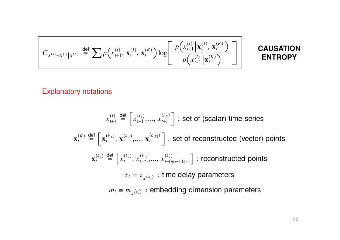
CXJ→XI XKdef= ∑ p x t+1
I, x t
J, xt
Klog
p x t+1I
xtJ
, xtK
p x t+1I
xtK
x t+1I def
= x t+1i1 ,..., x t+1
i|I| : set of (scalar) time-series
xtK def
= xtk 1 , x t
k 2 ,..., xt
k |K | : set of reconstructed (vector) points
x tk l def
= x tk l, x t−τl
k l,..., x t−m l−1τl
k l : reconstructed points
τl ≡ τx k l
: time delay parameters
ml ≡ mx k l
: embedding dimension parameters
Explanatory notations
CAUSATION
ENTROPY
63
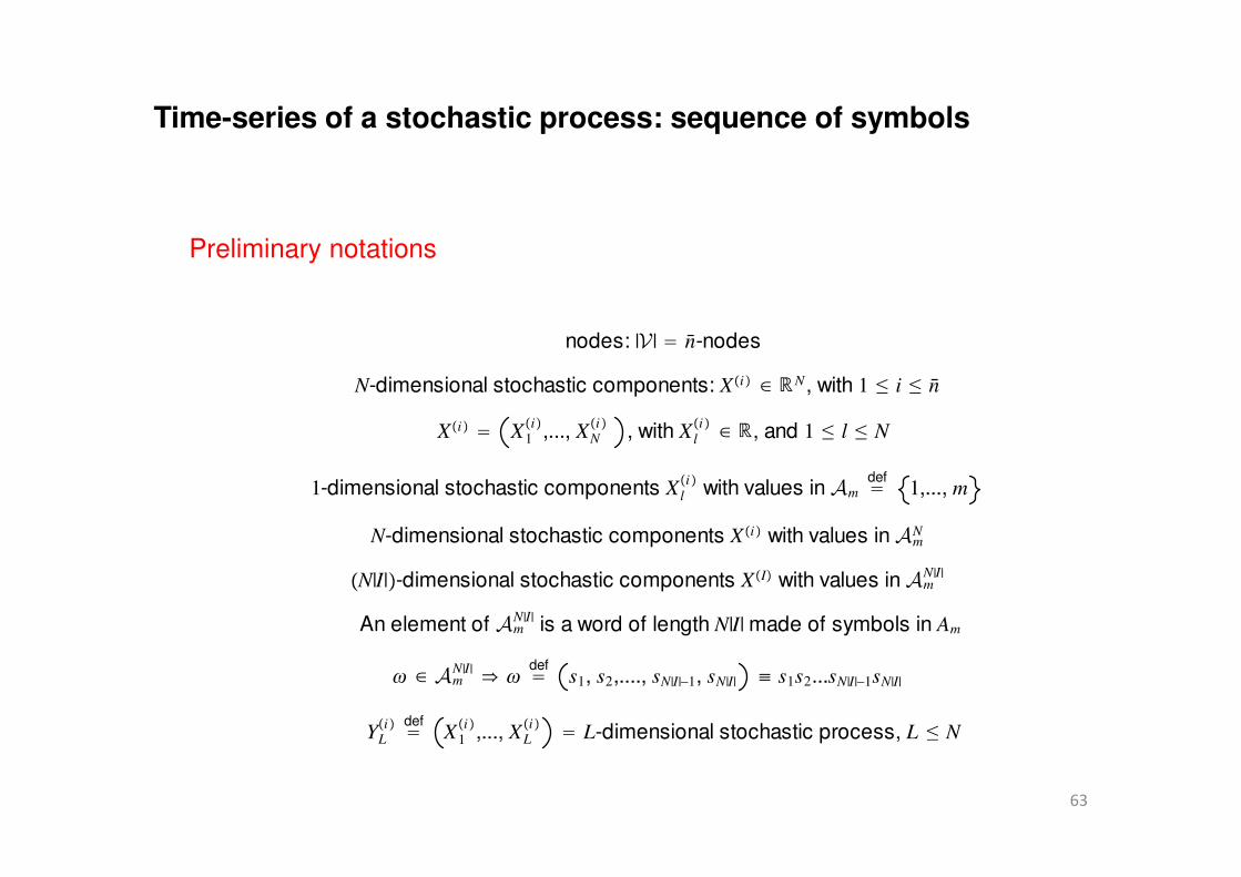
nodes: |V | = n-nodes
N-dimensional stochastic components: Xi ∈ ℝN, with 1 ≤ i ≤ n
Xi = X1i
,..., XNi
, with X l
i ∈ ℝ, and 1 ≤ l ≤ N
1-dimensional stochastic components X l
iwith values inAm
def= 1,..., m
N-dimensional stochastic components X i with values inAmN
N|I|-dimensional stochastic components XI with values inAmN|I|
An element of AmN|I| is a word of length N|I| made of symbols in Am
ω ∈ AmN|I| ⇒ ω
def= s1, s2,...., sN|I|−1, sN|I| ≡ s1s2...sN|I|−1sN|I|
YLi def
= X1i
,..., XLi
= L-dimensional stochastic process, L ≤ N
Time-series of a stochastic process: sequence of symbols
Preliminary notations

64
ĈXJ→XI XK def= ∑ p xt+1
I, xt
J, xt
Klog
p xt+1I
xtJ
, xtK
p xt+1I
xtK
CAUSATION
ENTROPY
xti
, sequence of symbols → xti
, sequence of observations
xt+1I
= sequence of symbols formed by the set of scalar time-series xt+1I
xtK
= sequence of symbols formed by the set of reconstructed vector points xtK
Explanatory notations

Summary: Part 3 (causal network inferenceand symbolic dynamics)
65
What did we do?
What is next?
Initial step: Formal construction of the symbolic Causation Entropy
Next steps: Practical estimation of symbolic Causation Entropy for bothsynthetic and real-world data
Relevance: Understand the link between dynamicalsystems and information-theoretic concepts
∑ ∑symbolization
(Expected) Relevance:• Less-demanding computational
cost for numerical estimations• Decrease of the negative effect
of observational noise in maskingthe details of the data-structure
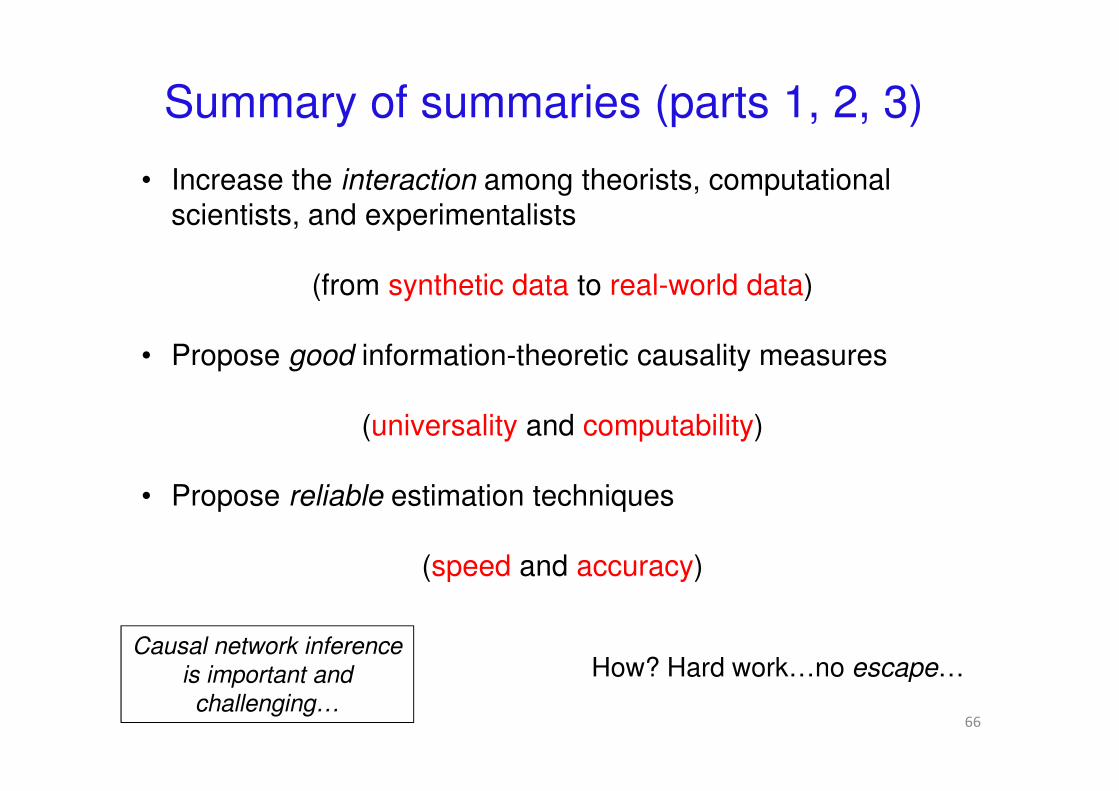
Summary of summaries (parts 1, 2, 3)
66
• Increase the interaction among theorists, computational
scientists, and experimentalists
(from synthetic data to real-world data)
• Propose good information-theoretic causality measures
(universality and computability)
• Propose reliable estimation techniques
(speed and accuracy)
How? Hard work…no escape…Causal network inference
is important and
challenging…

…On-going real-world applications of the CSE approach…
67
1. Swarm-data: information flow in a swarm of bugs…
2. Neuroimaging data (fMRI-functional magnetic resonance imaging): coupling structure between cerebral blood flow and neuralactivation…

68
References
The optimal Causation Entropy principle (oCSE principle)
• J. Sun and E. M. Bollt, Physica D267, 49 (2014)
• J. Sun, D. Taylor, and E. M. Bollt, arXiv:cs.IT/1401.7574 (2014)
• J. Sun, C. Cafaro, and E. M. Bollt, Entropy 16, 3416 (2014)
This work is funded by Army Research Office of
United States of America Grant No. 61386-EG
Acknowledgements

69
Thanks!