SWITCHED CONTROL STRATEGIES FOR UNDERACTUATED SYSTEMSbanavar/lectures/acods07_talk.pdf · Switched Control Strategies for Underactuated Systems Invited talk - ACODS07 Outline •

January 29, 2007

SWITCHED CONTROL STRATEGIES

FOR UNDERACTUATED SYSTEMS

R. N. Banavar

(Joint work with V. Sankaranarayanan)

Systems & Control Engg.

Indian Institute of Technology, Bombay

Mumbai -INDIA.

[email protected]

Switched Control Strategies

for Underactuated Systems Invited talk - ACODS07

Outline

• Nonintegrable constraints in mechanical systems, nonholonomic

systems and underactuated systems - a brief introduction

• Sliding modes and the switched control law philosophy

• Two examples

• Other issues of interest

1



Classification of constraints in mechanical systems

• Holonomic constraints - restrict the allowable configurations of the

system

• Nonintegrable constraints - do not restrict the allowable

configurations of the system but restrict instantaneous

velocities/accelerations

– Velocity level constraints - parking of a car, wheeled mobile robots,

rolling contacts in robotic applications

– Acceleration level constraints - fuel slosh in spacecrafts/launch

vehicles, underwater vehicles, underactuated mechanisms (on

purpose or loss of actuator) systems - serial link manipulators

Underactuated systems

2



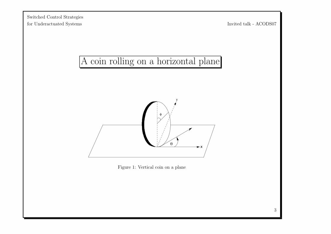
A coin rolling on a horizontal plane

x

y

θ

φ

Figure 1: Vertical coin on a plane

3


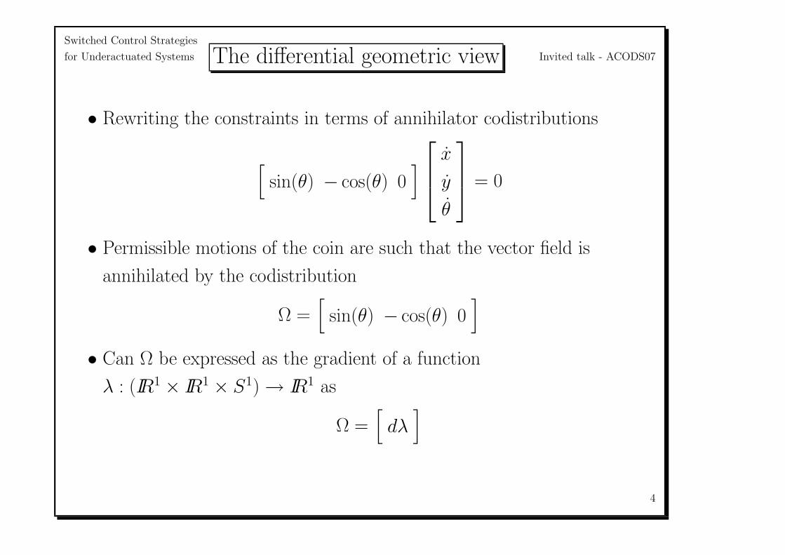
for Underactuated Systems Invited talk - ACODS07The differential geometric view

• Rewriting the constraints in terms of annihilator codistributions

[sin(θ) − cos(θ) 0

] x

y

θ

= 0

• Permissible motions of the coin are such that the vector field is

annihilated by the codistribution

Ω =[

sin(θ) − cos(θ) 0]

• Can Ω be expressed as the gradient of a function

λ : (IR1 × IR1 × S1) → IR1 as

Ω =[

dλ]

4



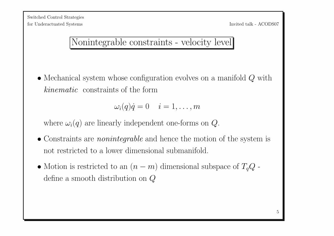
Nonintegrable constraints - velocity level

• Mechanical system whose configuration evolves on a manifold Q with

kinematic constraints of the form

ωi(q)q = 0 i = 1, . . . , m

where ωi(q) are linearly independent one-forms on Q.

• Constraints are nonintegrable and hence the motion of the system is

not restricted to a lower dimensional submanifold.

• Motion is restricted to an (n − m) dimensional subspace of TqQ -

define a smooth distribution on Q

5



Nonintegrable constraints - acceleration level

• Consider the manifold TQ and look at dynamic constraints of the form

αi(x)x = 0 i = 1, . . . , p

where x= (q, vq) are local coordinates for TQ, the αis are linearly

independent one-forms on TQ and vq= q.

• Constraints are nonintegrable and hence the motion of the system is

not restricted to a lower dimensional submanifold of TQ.

• The motion here is restricted at the acceleration level to an (n − p)

dimensional subspace of Tx(TQ) - define a smooth distribution on TQ

6



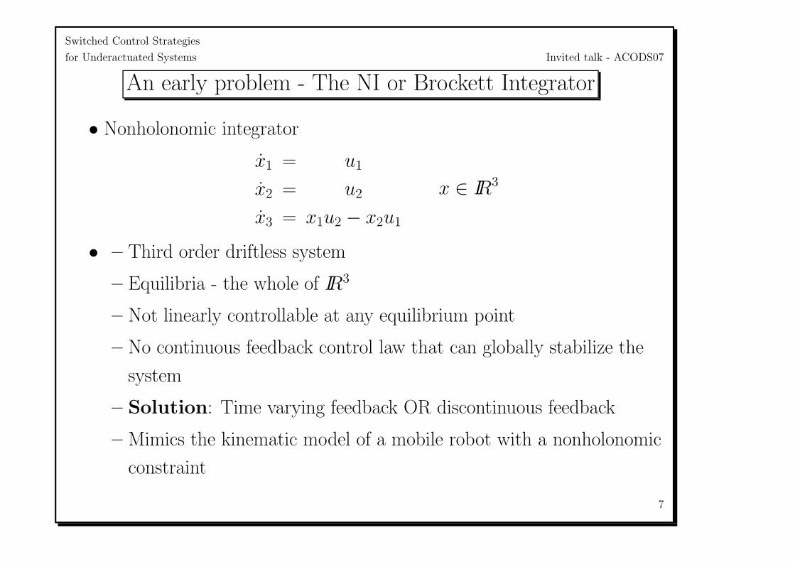
An early problem - The NI or Brockett Integrator

• Nonholonomic integrator

x1 = u1

x2 = u2

x3 = x1u2 − x2u1

x ∈ IR3

• – Third order driftless system

– Equilibria - the whole of IR3

– Not linearly controllable at any equilibrium point

– No continuous feedback control law that can globally stabilize the

system

– Solution: Time varying feedback OR discontinuous feedback

– Mimics the kinematic model of a mobile robot with a nonholonomic

constraint

7



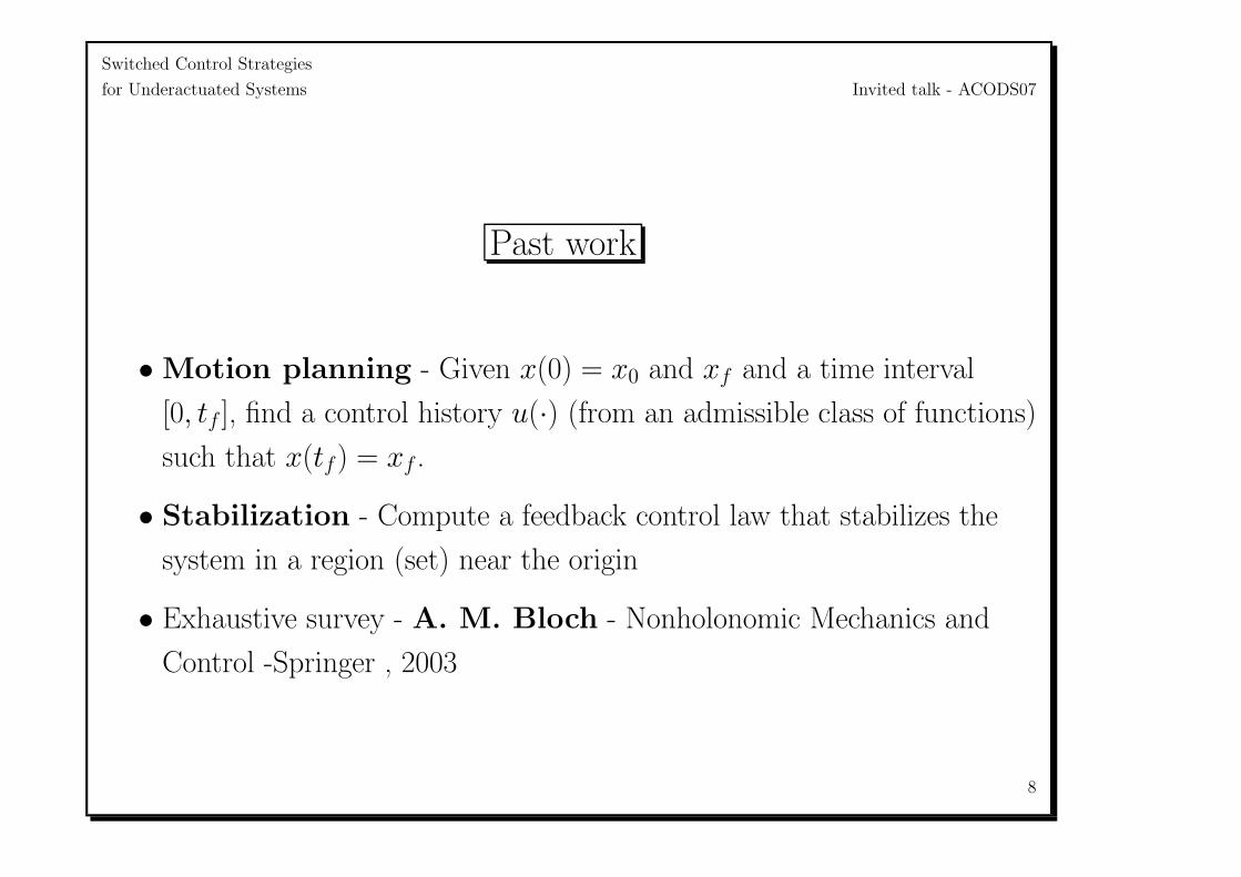
Past work

• Motion planning - Given x(0) = x0 and xf and a time interval

[0, tf ], find a control history u(·) (from an admissible class of functions)

such that x(tf) = xf .

• Stabilization - Compute a feedback control law that stabilizes the

system in a region (set) near the origin

• Exhaustive survey - A. M. Bloch - Nonholonomic Mechanics and

Control -Springer , 2003

8



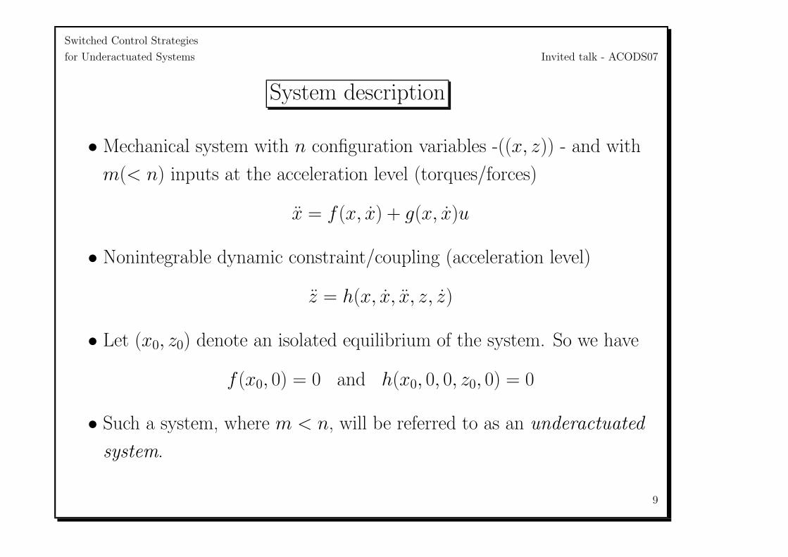
System description

• Mechanical system with n configuration variables -((x, z)) - and with

m(< n) inputs at the acceleration level (torques/forces)

x = f (x, x) + g(x, x)u

• Nonintegrable dynamic constraint/coupling (acceleration level)

z = h(x, x, x, z, z)

• Let (x0, z0) denote an isolated equilibrium of the system. So we have

f (x0, 0) = 0 and h(x0, 0, 0, z0, 0) = 0

• Such a system, where m < n, will be referred to as an underactuated

system.

9



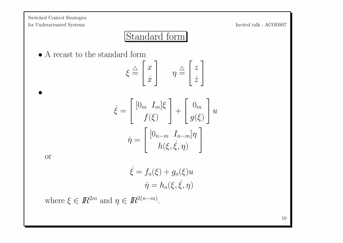
Standard form

• A recast to the standard form

ξ=

[x

x

]η

=

[z

z

]•

ξ =

[[0m Im]ξ

f (ξ)

]+

[0m

g(ξ)

]u

η =

[[0n−m In−m]η

h(ξ, ξ, η)

]or

ξ = fa(ξ) + ga(ξ)u

η = ha(ξ, ξ, η)

where ξ ∈ IR2m and η ∈ IR2(n−m).

10



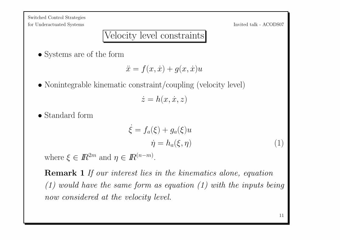
Velocity level constraints

• Systems are of the form

x = f (x, x) + g(x, x)u

• Nonintegrable kinematic constraint/coupling (velocity level)

z = h(x, x, z)

• Standard form

ξ = fa(ξ) + ga(ξ)u

η = ha(ξ, η) (1)

where ξ ∈ IR2m and η ∈ IR(n−m).

Remark 1 If our interest lies in the kinematics alone, equation

(1) would have the same form as equation (1) with the inputs being

now considered at the velocity level.

11



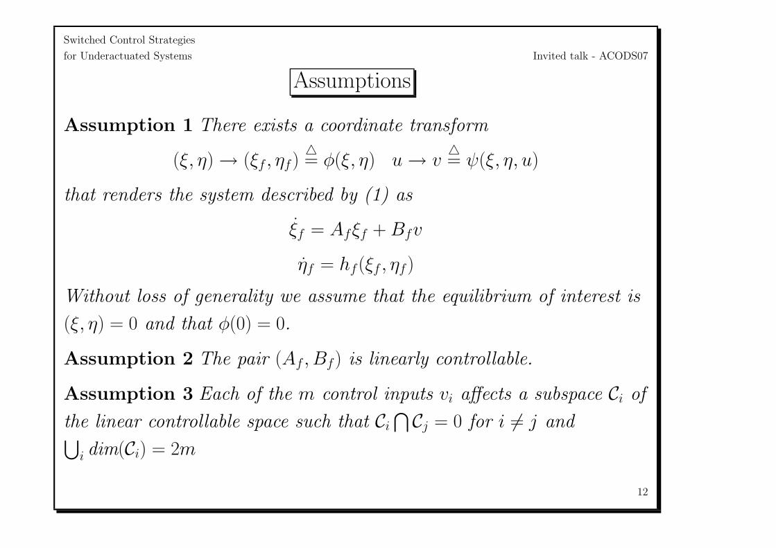
Assumptions

Assumption 1 There exists a coordinate transform

(ξ, η) → (ξf, ηf)= φ(ξ, η) u → v

= ψ(ξ, η, u)

that renders the system described by (1) as

ξf = Afξf + Bfv

ηf = hf(ξf, ηf)

Without loss of generality we assume that the equilibrium of interest is

(ξ, η) = 0 and that φ(0) = 0.

Assumption 2 The pair (Af, Bf) is linearly controllable.

Assumption 3 Each of the m control inputs vi affects a subspace Ci of

the linear controllable space such that Ci

⋂Cj = 0 for i = j and⋃

i dim(Ci) = 2m

12



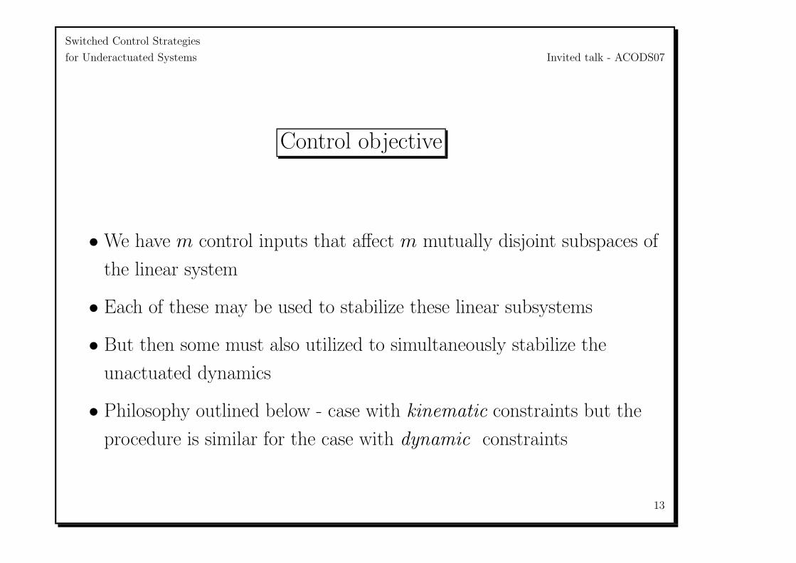
Control objective

• We have m control inputs that affect m mutually disjoint subspaces of

the linear system

• Each of these may be used to stabilize these linear subsystems

• But then some must also utilized to simultaneously stabilize the

unactuated dynamics

• Philosophy outlined below - case with kinematic constraints but the

procedure is similar for the case with dynamic constraints

13



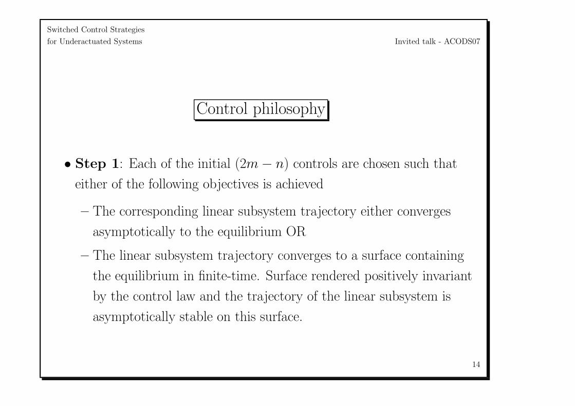
Control philosophy

• Step 1: Each of the initial (2m − n) controls are chosen such that

either of the following objectives is achieved

– The corresponding linear subsystem trajectory either converges

asymptotically to the equilibrium OR

– The linear subsystem trajectory converges to a surface containing

the equilibrium in finite-time. Surface rendered positively invariant

by the control law and the trajectory of the linear subsystem is

asymptotically stable on this surface.

14



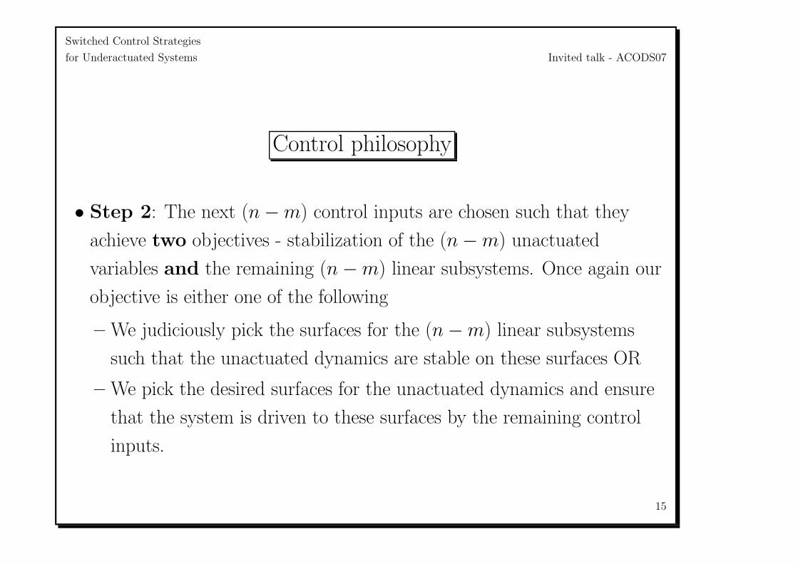
Control philosophy

• Step 2: The next (n − m) control inputs are chosen such that they

achieve two objectives - stabilization of the (n − m) unactuated

variables and the remaining (n − m) linear subsystems. Once again our

objective is either one of the following

– We judiciously pick the surfaces for the (n − m) linear subsystems

such that the unactuated dynamics are stable on these surfaces OR

– We pick the desired surfaces for the unactuated dynamics and ensure

that the system is driven to these surfaces by the remaining control

inputs.

15



Features of the control law

Two features of our proposed control laws, which are also their inherent

limitations, are

1. Avoidance of thin sets: They work with initial conditions starting in

an appropriate set. Notion of stability that we employ is termed

relative stability and we define these thin sets for every problem.

2. Switching: To avoid singularities and ensure that the states do not get

unbounded, we prescribe a switching strategy.

16



Finite time stabilization to the surface S(x) = 0

• The dynamics of the surface is given by

S = −ksS1/3 ks > 0

• Consider a Lyapunov candidate function and its rate of change

V = S2/2

V = −ksS4/3 < 0

Hence S = 0 is attractive globally.

• For finite time convergence we show

V + kV α ≤ 0 ([Haimo] condition for finite-time stability)

where α ∈ (0, 1) and k > 0

17



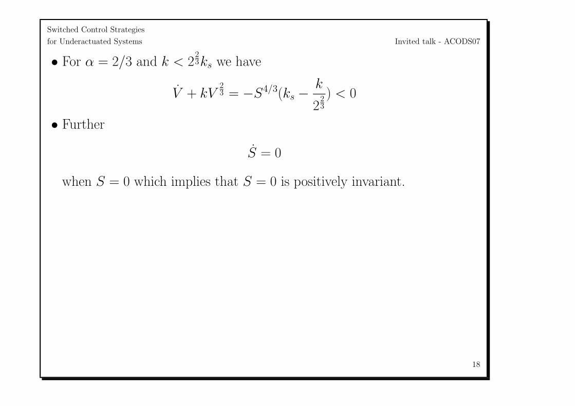
• For α = 2/3 and k < 223ks we have

V + kV23 = −S4/3(ks −

k

223

) < 0

• Further

S = 0

when S = 0 which implies that S = 0 is positively invariant.

18



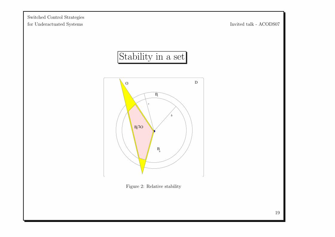
Stability in a set

D

Bε

Bδ

δ

ε

Bδ

U

O

O

Figure 2: Relative stability

19



A wheeled mobile robot on a horizontal plane

x

y

θ

τ1

τ 2

Figure 3: Schematic of a mobile robot

20



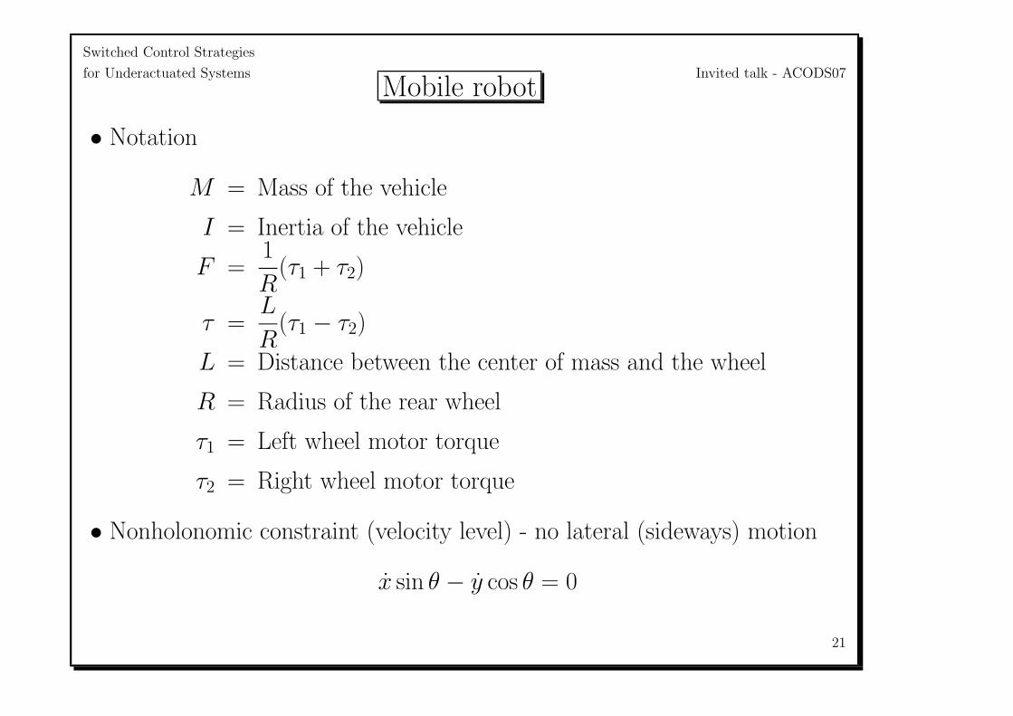
Mobile robot

• Notation

M = Mass of the vehicle

I = Inertia of the vehicle

F =1

R(τ1 + τ2)

τ =L

R(τ1 − τ2)

L = Distance between the center of mass and the wheel

R = Radius of the rear wheel

τ1 = Left wheel motor torque

τ2 = Right wheel motor torque

• Nonholonomic constraint (velocity level) - no lateral (sideways) motion

x sin θ − y cos θ = 0

21



Kinematics and Dynamics

• Generalized coordinates - position of the center of mass (x, y) and

orientation θ

• Constraints of motion

x sin θ − y cos θ = 0 No lateral motion

• Equations at the kinematic level

θ = ω x = v cos θ y = v sin θ

- drive v and steer ω

• Dynamics - (control inputs are forces and torques)

Mv = F

Iω = τ

22



Dynamic model of the mobile robot

• θ

x

y

v

ω

=

ω

v cos θ

v sin θ

0

0

+

0

0

01M

0

F +

0

0

0

01I

τ

• Fifth order system with drift

• With a coordinate transform, resembles the extended nonholonomic

double integrator

23



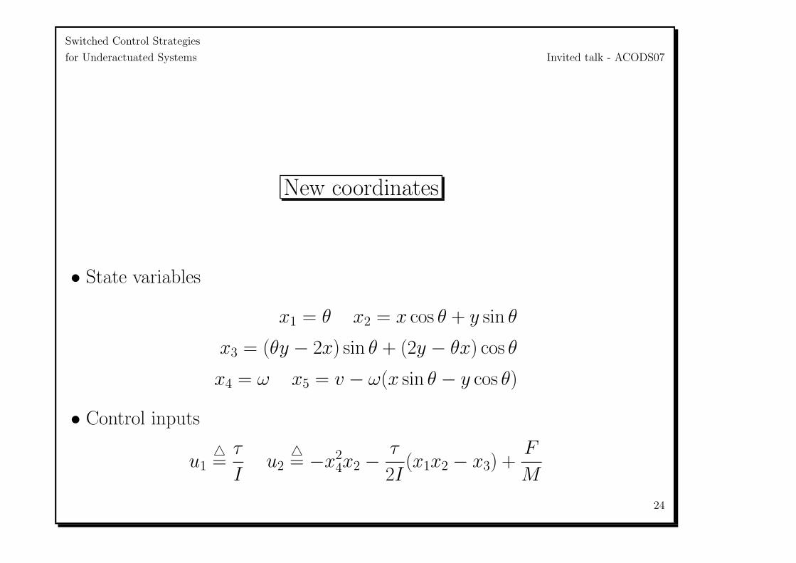
New coordinates

• State variables

x1 = θ x2 = x cos θ + y sin θ

x3 = (θy − 2x) sin θ + (2y − θx) cos θ

x4 = ω x5 = v − ω(x sin θ − y cos θ)

• Control inputs

u1=

τ

Iu2

= −x2

4x2 −τ

2I(x1x2 − x3) +

F

M

24



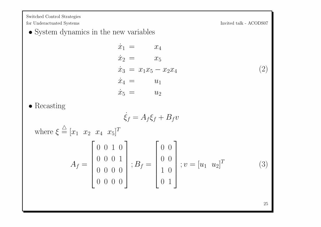
• System dynamics in the new variables

x1 = x4

x2 = x5

x3 = x1x5 − x2x4

x4 = u1

x5 = u2

(2)

• Recasting

ξf = Afξf + Bfv

where ξ= [x1 x2 x4 x5]

T

Af =

0 0 1 0

0 0 0 1

0 0 0 0

0 0 0 0

; Bf =

0 0

0 0

1 0

0 1

; v = [u1 u2]T (3)

25



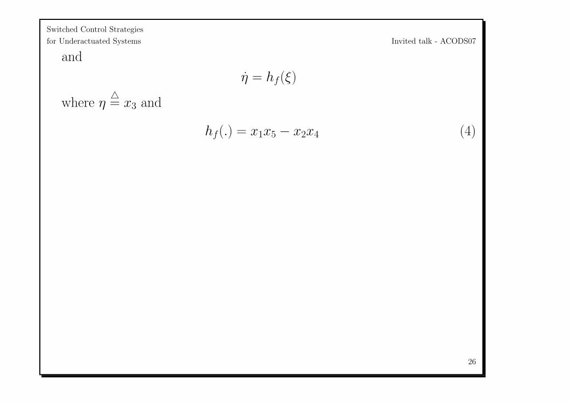
and

η = hf(ξ)

where η= x3 and

hf(.) = x1x5 − x2x4 (4)

26



The Extended Nonholonomic Double Integrator (ENDI)

x = f (x) +

2∑i=1

gi(x)ui

where x= [x1, x2, x3, y1, y2]

T ∈ IR5 is the state vector and

u= [u1, u2] ∈ IR2 is the control

f (x)=

y1

y2

x1y2 − x2y1

0

0

; g1(x)=

0

0

0

1

0

; g2(x)=

0

0

0

0

1

27



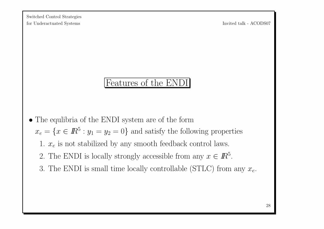
Features of the ENDI

• The equlibria of the ENDI system are of the form

xe = x ∈ IR5 : y1 = y2 = 0 and satisfy the following properties

1. xe is not stabilized by any smooth feedback control laws.

2. The ENDI is locally strongly accessible from any x ∈ IR5.

3. The ENDI is small time locally controllable (STLC) from any xe.

28



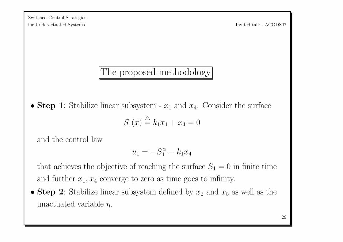
The proposed methodology

• Step 1: Stabilize linear subsystem - x1 and x4. Consider the surface

S1(x)= k1x1 + x4 = 0

and the control law

u1 = −Sα1 − k1x4

that achieves the objective of reaching the surface S1 = 0 in finite time

and further x1, x4 converge to zero as time goes to infinity.

• Step 2: Stabilize linear subsystem defined by x2 and x5 as well as the

unactuated variable η.

29



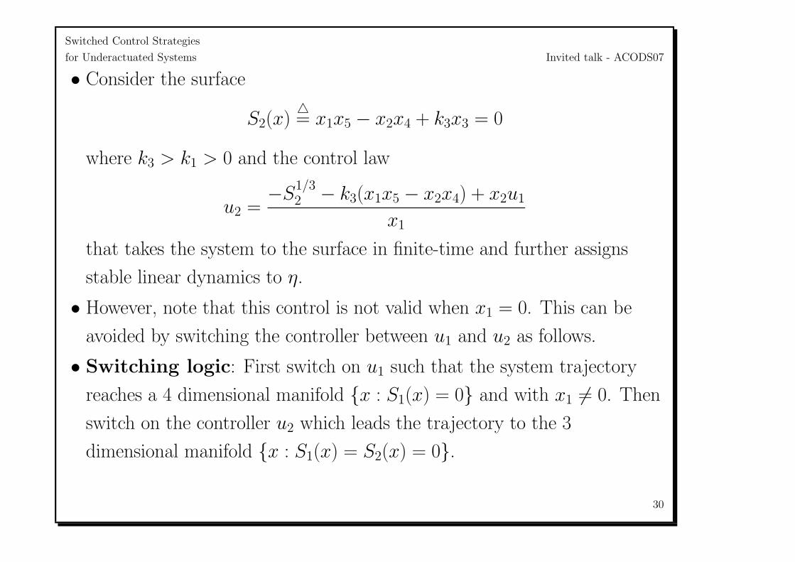
• Consider the surface

S2(x)= x1x5 − x2x4 + k3x3 = 0

where k3 > k1 > 0 and the control law

u2 =−S

1/32 − k3(x1x5 − x2x4) + x2u1

x1

that takes the system to the surface in finite-time and further assigns

stable linear dynamics to η.

• However, note that this control is not valid when x1 = 0. This can be

avoided by switching the controller between u1 and u2 as follows.

• Switching logic: First switch on u1 such that the system trajectory

reaches a 4 dimensional manifold x : S1(x) = 0 and with x1 = 0. Then

switch on the controller u2 which leads the trajectory to the 3

dimensional manifold x : S1(x) = S2(x) = 0.

30



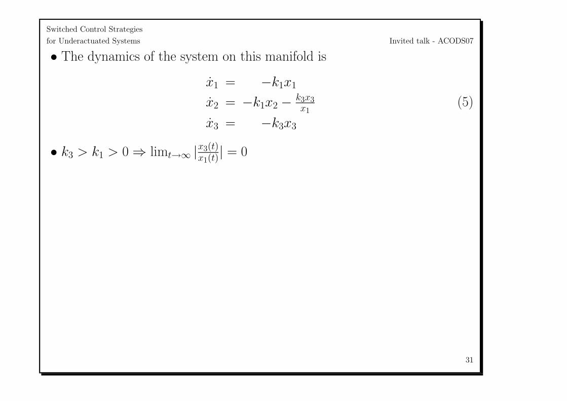
• The dynamics of the system on this manifold is

x1 = −k1x1

x2 = −k1x2 − k3x3x1

x3 = −k3x3

(5)

• k3 > k1 > 0 ⇒ limt→∞ |x3(t)x1(t)

| = 0

31



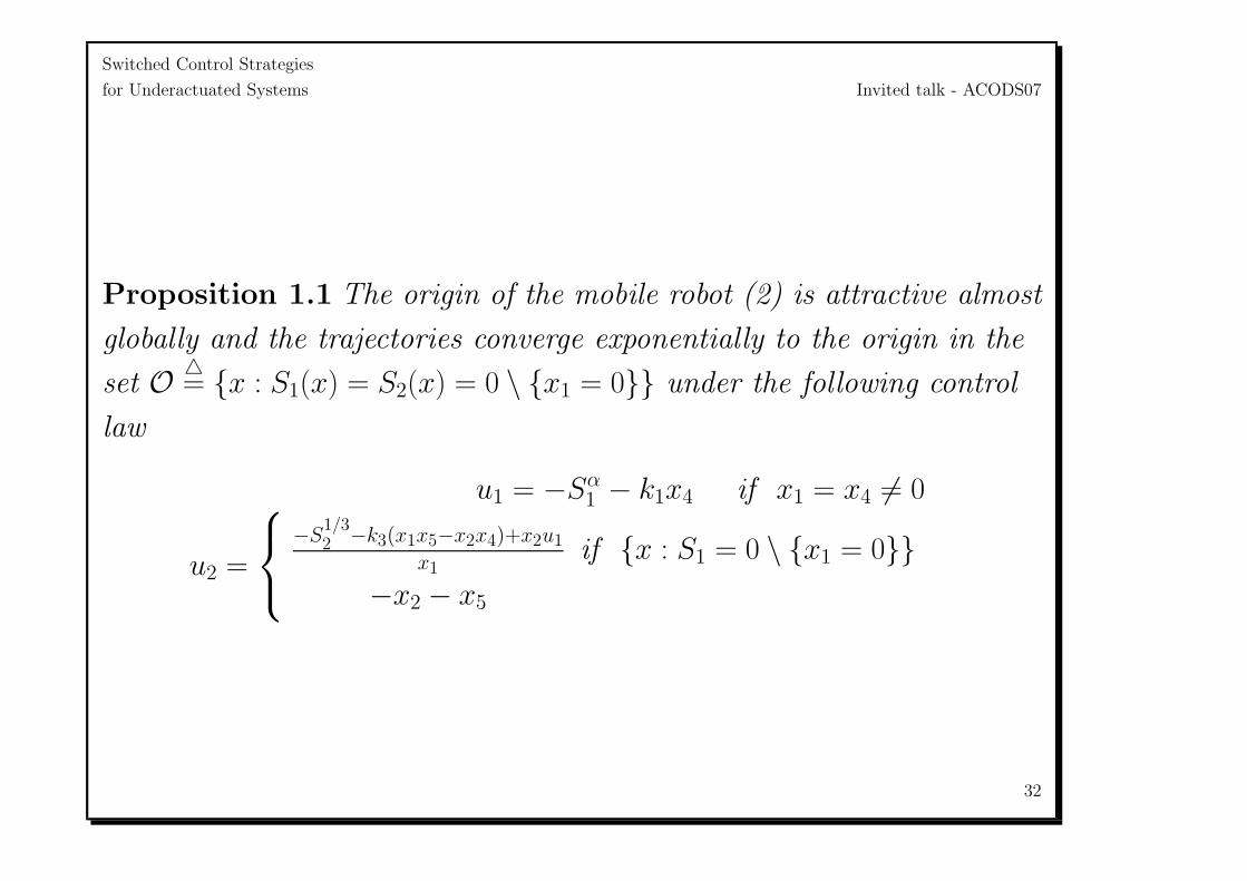
Proposition 1.1 The origin of the mobile robot (2) is attractive almost

globally and the trajectories converge exponentially to the origin in the

set O = x : S1(x) = S2(x) = 0 \ x1 = 0 under the following control

law

u1 = −Sα1 − k1x4 if x1 = x4 = 0

u2 =

−S1/32 −k3(x1x5−x2x4)+x2u1

x1if x : S1 = 0 \ x1 = 0

−x2 − x5

32



Simulation

• Initial conditions are x(0) = −1.5m, y(0) = 4m, θ(0) = −2.3rad, ω(0) =

1rad/sec, v(0) = −1m/sec.

• Controller parameters are k = 0.5, k3 = 1.

• Vehicle parameters are M = 10Kg, I = 2Kgm2, L = 6cm, R = 3cm.

33



34



0 10 20 30 40 50−4

−2

0

2

4

6

time in sec

x,y,θ

0 10 20 30 40 50−1

−0.5

0

0.5

1

1.5

time in sec

v,ω

0 10 20 30 40 50−0.2

−0.15

−0.1

−0.05

0

0.05

0.1

0.15

time in sec

τ 1,τ2

0 10 20 30 40 50−2

0

2

4

6

8

time in sec

S1,S

2

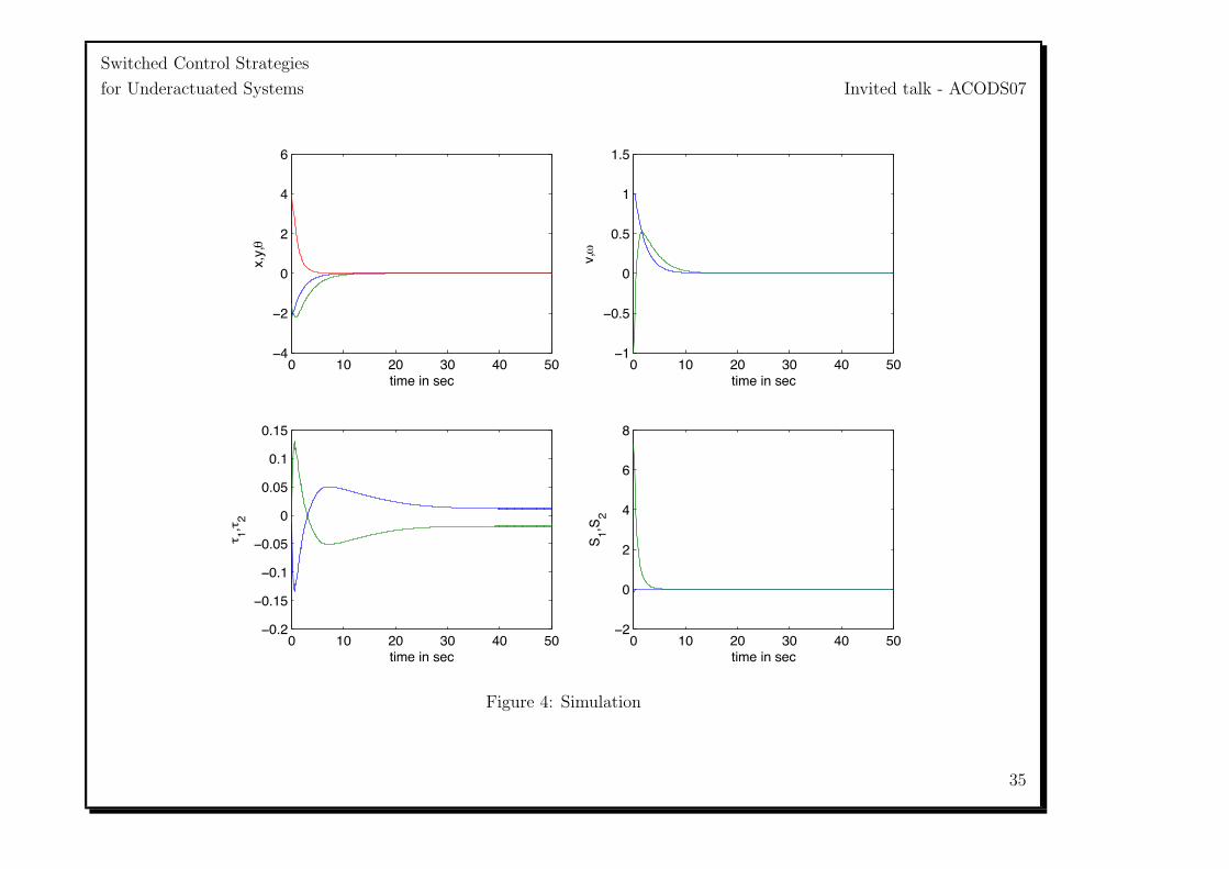
Figure 4: Simulation

35



36



−5 −4 −3 −2 −1 0 1 2 3 4 5−5

−4

−3

−2

−1

0

1

2

3

4

5

initial configuration

final configuration

x in meters

y in

met

ers

Figure 5: Stabilization to the origin

37



38



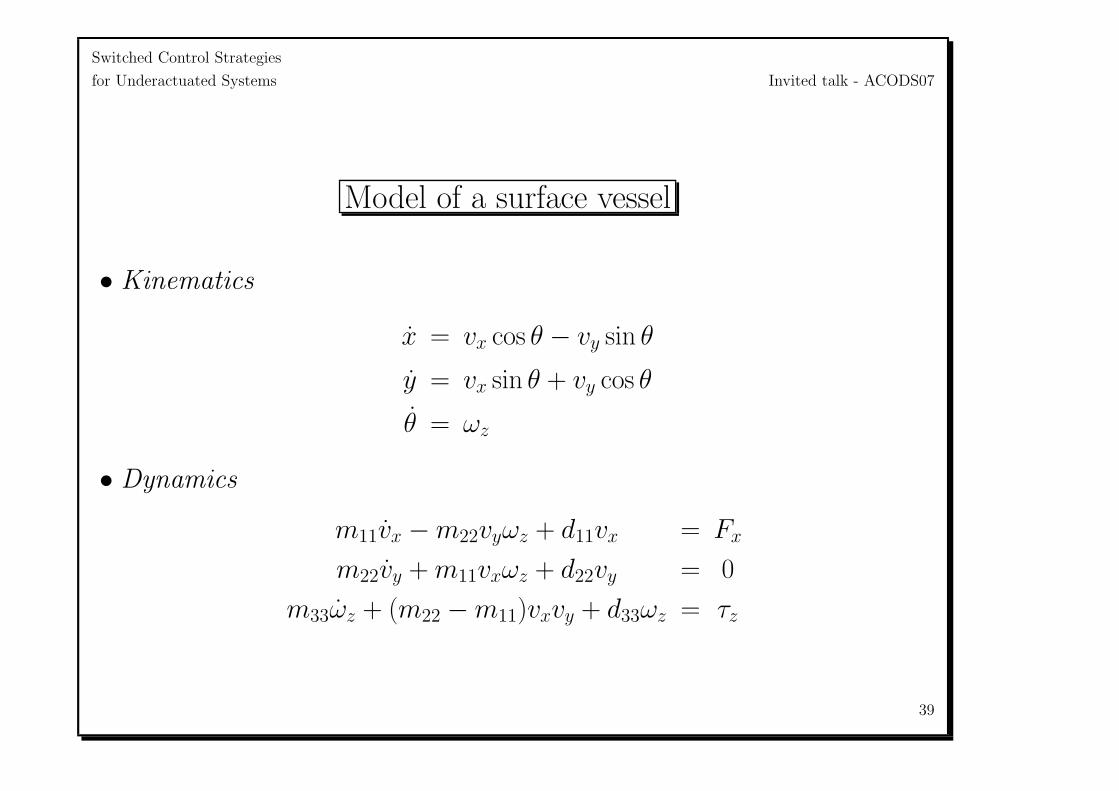
Model of a surface vessel

• Kinematics

x = vx cos θ − vy sin θ

y = vx sin θ + vy cos θ

θ = ωz

• Dynamics

m11vx − m22vyωz + d11vx = Fx

m22vy + m11vxωz + d22vy = 0

m33ωz + (m22 − m11)vxvy + d33ωz = τz

39



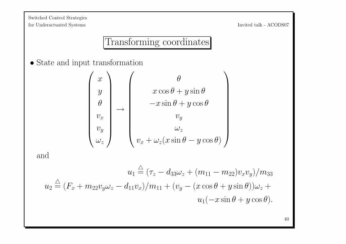
Transforming coordinates

• State and input transformation

x

y

θ

vx

vy

ωz

→

θ

x cos θ + y sin θ

−x sin θ + y cos θ

vy

ωz

vx + ωz(x sin θ − y cos θ)

and

u1= (τz − d33ωz + (m11 − m22)vxvy)/m33

u2= (Fx + m22vyωz − d11vx)/m11 + (vy − (x cos θ + y sin θ))ωz +

u1(−x sin θ + y cos θ).

40



The system in new coordinates

• Two linear subsystems and the unactuated subsystem as

x1

x2

x3

x4

x5

x6

=

x5

x6

x4 − x2x5

−αx4 + β(x25x3) − βx5x6

u1

u2

(6)

where α= d22

m22and β = m11

m22

41



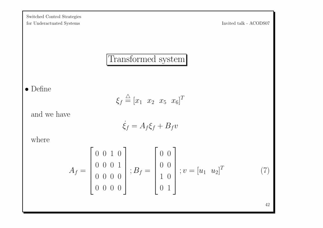
Transformed system

• Define

ξf= [x1 x2 x5 x6]

T

and we have

ξf = Afξf + Bfv

where

Af =

0 0 1 0

0 0 0 1

0 0 0 0

0 0 0 0

; Bf =

0 0

0 0

1 0

0 1

; v = [u1 u2]T (7)

42



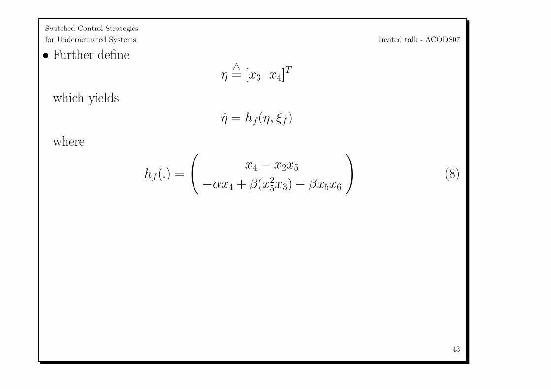
• Further define

η= [x3 x4]

T

which yields

η = hf(η, ξf)

where

hf(.) =

(x4 − x2x5

−αx4 + β(x25x3) − βx5x6

)(8)

43



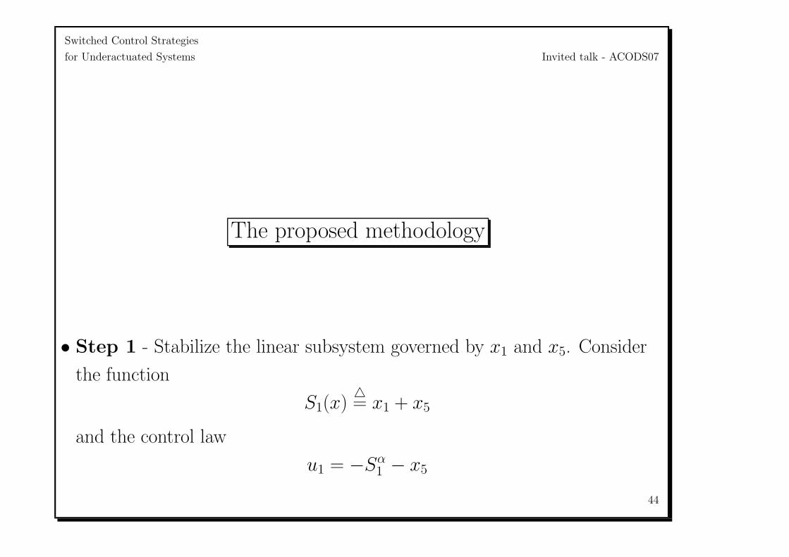
The proposed methodology

• Step 1 - Stabilize the linear subsystem governed by x1 and x5. Consider

the function

S1(x)= x1 + x5

and the control law

u1 = −Sα1 − x5

44



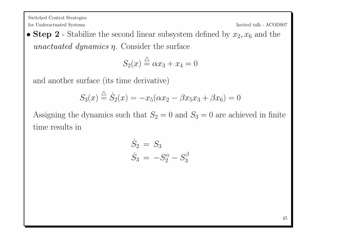
• Step 2 - Stabilize the second linear subsystem defined by x2, x6 and the

unactuated dynamics η. Consider the surface

S2(x)= αx3 + x4 = 0

and another surface (its time derivative)

S3(x)= S2(x) = −x5(αx2 − βx5x3 + βx6) = 0

Assigning the dynamics such that S2 = 0 and S3 = 0 are achieved in finite

time results in

S2 = S3

S3 = −Sα2 − Sβ

3

45



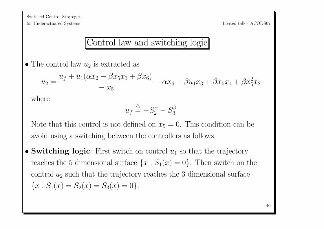
Control law and switching logic

• The control law u2 is extracted as

u2 =uf + u1(αx2 − βx5x3 + βx6)

− x5− αx6 + βu1x3 + βx5x4 + βx2

5x2

where

uf= −Sα

2 − Sβ3

Note that this control is not defined on x5 = 0. This condition can be

avoid using a switching between the controllers as follows.

• Switching logic: First switch on control u1 so that the trajectory

reaches the 5 dimensional surface x : S1(x) = 0. Then switch on the

control u2 such that the trajectory reaches the 3 dimensional surface

x : S1(x) = S2(x) = S3(x) = 0.

46



Stability

• The dynamics on this 3 dimensional surface is

x1 = −x1

x2 = −αβx2 + x3x5

x3 = −αx3 − x2x5

(9)

• Using the Lyapunov candidate function

V (x) =x2

1

2+

x22

2+

x23

2and its time derivative

V (x) = −x21 −

α

βx2

2 − αx23

< 0 ∀x = 0

and V = 0 only when x = 0.

47



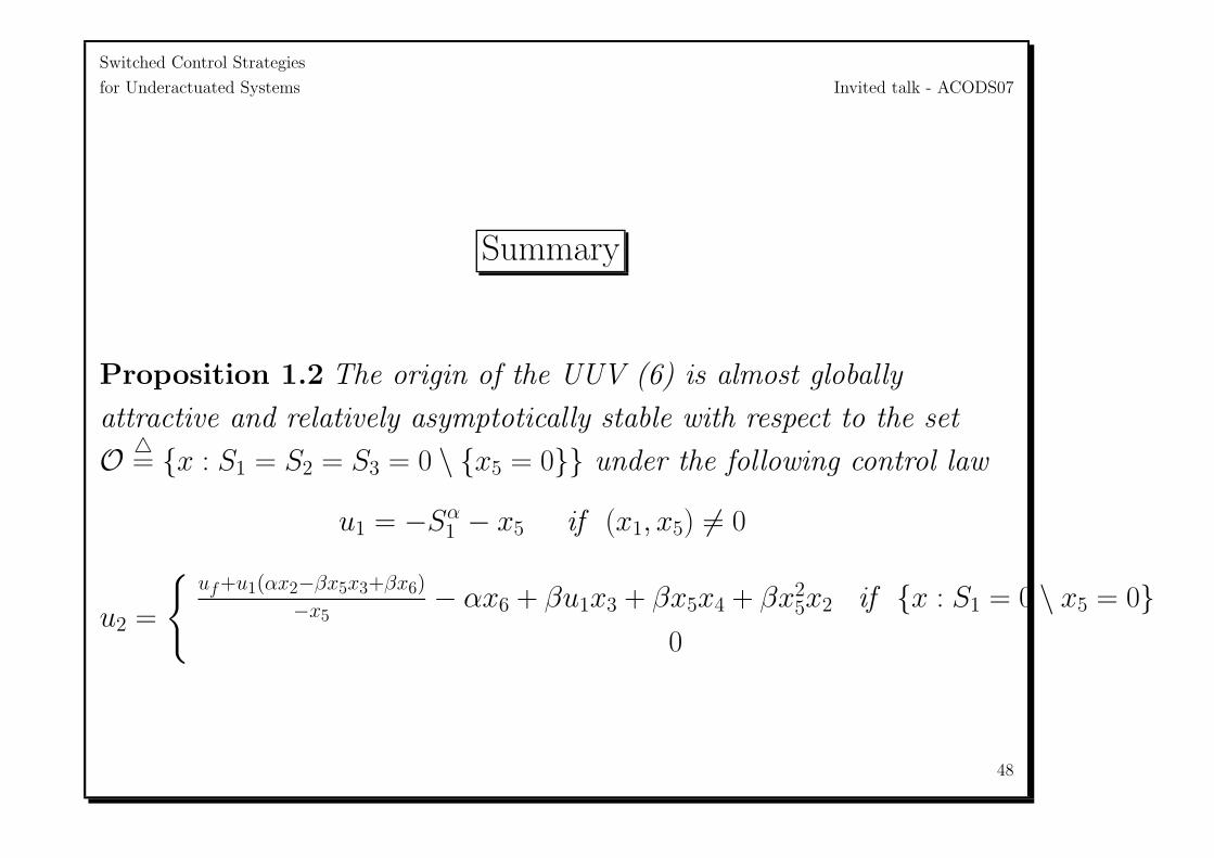
Summary

Proposition 1.2 The origin of the UUV (6) is almost globally

attractive and relatively asymptotically stable with respect to the set

O = x : S1 = S2 = S3 = 0 \ x5 = 0 under the following control law

u1 = −Sα1 − x5 if (x1, x5) = 0

u2 =

uf+u1(αx2−βx5x3+βx6)

−x5− αx6 + βu1x3 + βx5x4 + βx2

5x2 if x : S1 = 0 \ x5 = 00 o

48



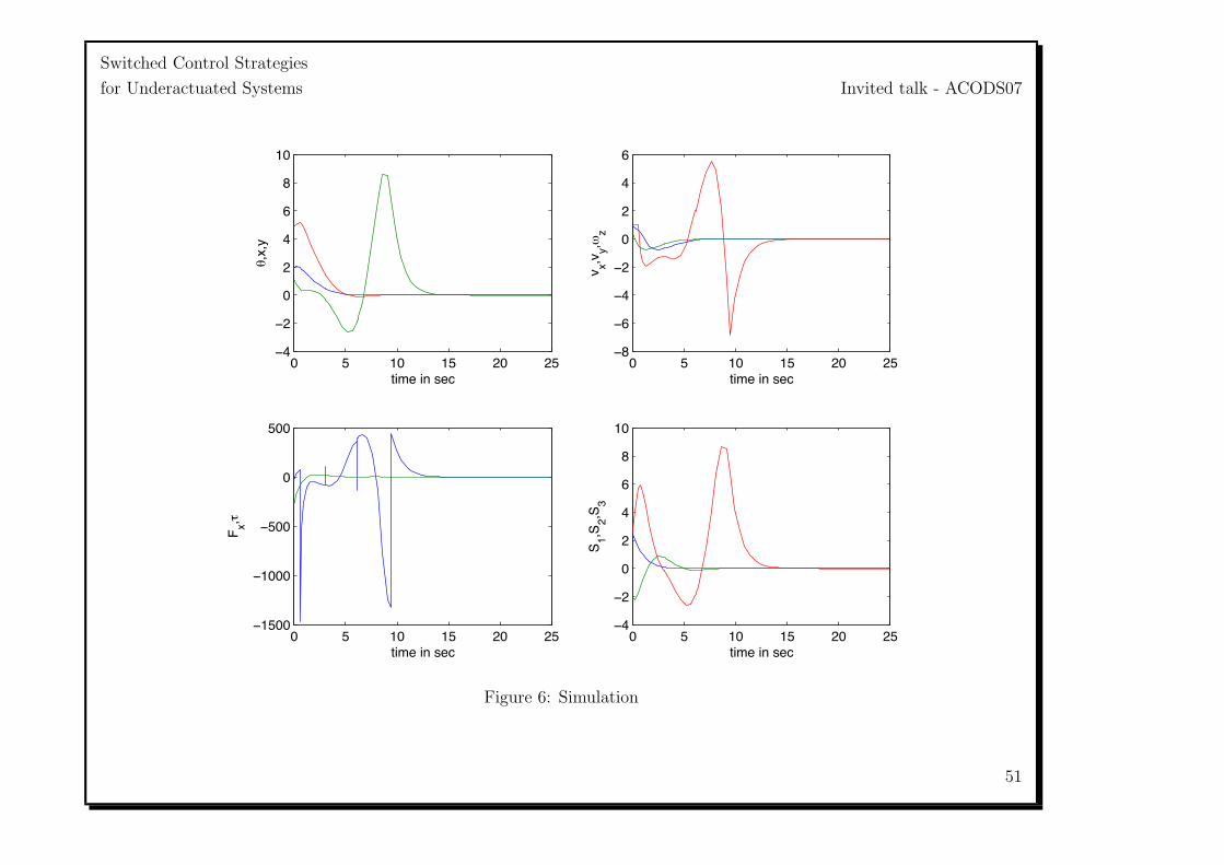
Simulation

• Initial conditions - θ(0) = 2rad/sec, x(0) = 1m, y(0) = 5m, vx(0) =

m/sec, ωz(0) = 0.5rad/sec, vy(0) = 1m/sec

• Vehicle parameters are

m11 = 100, m22 = 125, m33 = d11 = 35, d22 = 100, d33 = 50

49



50



0 5 10 15 20 25−4

−2

0

2

4

6

8

10

time in sec

θ,x,

y

0 5 10 15 20 25−8

−6

−4

−2

0

2

4

6

time in sec

v x,vy,ω

z

0 5 10 15 20 25−1500

−1000

−500

0

500

time in sec

Fx,τ

0 5 10 15 20 25−4

−2

0

2

4

6

8

10

time in sec

S1,S

2,S3

Figure 6: Simulation

51



Thank You

52

Documents

SWITCHED CONTROL STRATEGIES FOR UNDERACTUATED SYSTEMSbanavar/lectures/acods07_talk.pdf · Switched Control Strategies for Underactuated Systems Invited talk - ACODS07 Outline •