Swinburne University of

Technology

Doctoral Thesis

Dissipation

in

Oscillating Water Columns

Author:

Md Kamrul Hasan

Supervisors:

A/Prof Richard Manasseh

Dr Justin Leontini

A/Prof Alessandro Toffoli

Prof Alexander Babanin

April 23, 2017

Abstract

The Oscillating Water Column (OWC), regarded as the first generation Wave

Energy Converter (WEC), is one of the most effective technologies for extraction

of ocean wave energy. Most OWCs are designed to resonate at incoming wave

frequencies, so that efficiency of the device would be the maximum. In practice,

the eigenperiod of OWCs is too small with respect to most energetic waves, owing

to practicalities of construction and deployment, so the theoretical maximum is not

attained. Moreover, the damping factors, which control the actual value of this

maximum, are not clearly identified and modelled. Therefore, an extensive study of

the internal fluid dynamics of an OWC is required to identify those damping factors,

and furthermore, to estimate the amount of energy loss due to their presence in

OWCs.

Analytic models incorporating viscous and turbulent boundary-layer dissipation

in a fixed-type OWC are derived from the Navier-Stokes equations. The OWC is

modelled as a partially submerged straight circular cross-section pipe. The origin of

the dissipation terms in the momentum conservation equations are explicitly iden-

tified. The contributions of different damping sources to the overall energy loss are

compared. As a first approximation, the flow inside the device is assumed fully devel-

oped along the entire length, to eliminate the effect of the flow development region.

The Power-Take-Off (PTO) system is modelled assuming that the air compresses

and expands isentropically in the air chamber. Theory developed in [1] for comput-

ing the hydrodynamic coefficients related to the scattered wave and radiation wave

is adapted into the present models. A novel contribution of the present work is the

inclusion of damping due to the wall shear stress, modelled for the reciprocating flow

system inside the OWC. It is found that damping due to the radiation wave is the

largest damping source if the draft (submergence depth) of the device is relatively

short. However, with the increase of the draft, radiation damping becomes weaker.

Conversely, the wall shear stress damping becomes stronger with the increase of the

draft.

For the analytical study, it is assumed that the flow is fully developed throughout

the device. However, in reality, there is a significant flow development region in a

typical OWC. Unlike unidirectional flow, there is no established correlation between

the Reynolds number and the flow developing length in reciprocating flow. Thus

a numerical study is conducted with a Direct Numerical Simulation (DNS) code

to investigate the flow developing length in reciprocating pipe flow. It is found

that the developing length varies periodically in the cycle. Linear correlations are

presented to estimate the maximum and cycle-average developing lengths ((le)max

and (le)mean) from the Reynolds number Reδ = U0δ/ν, where U0 = cross-sectional

mean velocity amplitude and δ =√

2ν/ω = Stokes layer thickness.

It is confirmed that the developing length in reciprocating pipe flow is not in-

significant. Hence, an approach is taken to measure the energy loss due to the

free-end in a pipe with the same DNS code which has been used to measure the

developing length. It is found that in a long pipe, the loss owing to the internal

shear stress dominates over the free-end loss. However, as the pipe gets shorter, the

domination of internal shear stress loss decreases and the portion of the free-end loss

in the overall loss increases. It is shown that for a 5-diameter long pipe if Reδ > 80,

the free-end loss dominates over the internal shear stress loss. Vortex formation due

to the free-end and its corresponding energy dissipation field are visualised. It is

found that within a few diameters downstream from the free-end the vortices be-

come so weak that the dissipation caused by the vortices far outside the free-end is

insignificant.

Finally, analytical models for a fixed-type tuned Oscillating Water Column (OWC)

device are derived. This is an example of an application of the research in the fore-

going Chapters. A variable volume air-compression chamber is used as the tuning

system. The shear stress and radiation damping terms in the equations of motion

are modelled in a similar manner to the single column OWC mentioned above. The

free-end damping term is incorporated from the DNS study. It is found that the

introduction of free-end damping reduces the overall power output of the device

significantly.

To those, who born poor, live poor, and die poor.

Acknowledgements

I would like to express my sincere gratitude to my supervisor, A/Prof. Richard

Manasseh, for his guidance, teaching, time, and above all for being patient and

very nice to me throughout the period of my study. Whenever I was stuck, his

motivational words inspired me to overcome the difficulties, rather than just giving

up. I also would like to express my deep gratitude to another supervisor, Dr Justin

Leontini, for his time, friendly teaching, and never ending inspiration. I barely

know any supervisor like him who tries to manage time for his students almost

everyday, depending on their needs. I would like to thank my family members for

their constant supports, even though they were 8903 km away from me. Finally, I

am very grateful to all my friends who were always supportive to me to complete

this study.

Declaration of Authorship

This thesis contains no material which has been accepted for the award of any other

degree or diploma. To the best of my knowledge, this thesis contains no material

previously published or written by another person except where due reference is

made in the text.

Signed:

Date:

Contents

1 Introduction 1

2 Literature Review 8

2.1 Background of OWCs . . . . . . . . . . . . . . . . . . . . . . . . . . . 9

2.2 Theoretical modelling of OWCs . . . . . . . . . . . . . . . . . . . . . 11

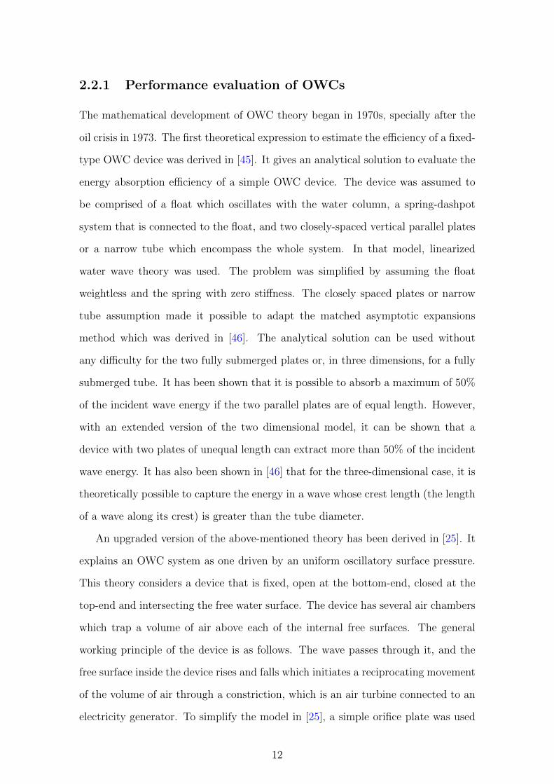
2.2.1 Performance evaluation of OWCs . . . . . . . . . . . . . . . . 12

2.2.2 Tuning mechanisms of OWC devices . . . . . . . . . . . . . . 16

2.3 Reciprocating pipe flow . . . . . . . . . . . . . . . . . . . . . . . . . . 20

2.3.1 Flow characteristics and transition from laminar to turbulent . 21

2.3.2 Entrance length . . . . . . . . . . . . . . . . . . . . . . . . . . 29

2.3.3 Energy loss due to shear stress and entrance effects . . . . . . 30

3 Analytic representations of dissipation in OWCs 37

3.1 Formulation . . . . . . . . . . . . . . . . . . . . . . . . . . . . . . . . 39

3.1.1 Simplifying the x-momentum equation of the water column . . 41

3.1.2 Modelling the wall shear stress, τw(t) in the reciprocating flow

system of the OWC . . . . . . . . . . . . . . . . . . . . . . . . 44

3.1.3 Modelling the Power-Take-Off (PTO) . . . . . . . . . . . . . . 47

3.2 Results . . . . . . . . . . . . . . . . . . . . . . . . . . . . . . . . . . . 48

3.3 Summary . . . . . . . . . . . . . . . . . . . . . . . . . . . . . . . . . 55

4 Entrance length in laminar reciprocating pipe flow 57

4.1 Validation . . . . . . . . . . . . . . . . . . . . . . . . . . . . . . . . . 61

4.2 Measuring the entrance length . . . . . . . . . . . . . . . . . . . . . . 62

i

4.2.1 Measuring techniques . . . . . . . . . . . . . . . . . . . . . . . 64

4.2.2 Comparing the measurement techniques . . . . . . . . . . . . 66

4.3 Results . . . . . . . . . . . . . . . . . . . . . . . . . . . . . . . . . . . 67

4.4 Summary . . . . . . . . . . . . . . . . . . . . . . . . . . . . . . . . . 73

5 Dissipation due to a free-end in reciprocating pipe flow 75

5.1 Formulation . . . . . . . . . . . . . . . . . . . . . . . . . . . . . . . . 78

5.2 Validation . . . . . . . . . . . . . . . . . . . . . . . . . . . . . . . . . 83

5.3 Results . . . . . . . . . . . . . . . . . . . . . . . . . . . . . . . . . . . 84

5.3.1 Energy loss in the entire domain, ˙Eew . . . . . . . . . . . . . . 85

5.3.2 Energy loss due to a fully developed flow throughout the pipe,

˙Ew . . . . . . . . . . . . . . . . . . . . . . . . . . . . . . . . . 86

5.3.3 Energy loss due to the free-end, ˙Ee . . . . . . . . . . . . . . . 86

5.3.4 Energy loss outside the pipe due to the free-end, ˙Eeo . . . . . 89

5.3.5 Vorticity and energy dissipation fields around the free-end . . 91

5.3.6 Comparison between ˙Ew and ˙Ee for different pipe

lengths . . . . . . . . . . . . . . . . . . . . . . . . . . . . . . . 93

5.3.7 The total dissipation ˙Eew as a function of A0 at low and high α′ 95

5.4 Summary . . . . . . . . . . . . . . . . . . . . . . . . . . . . . . . . . 95

6 Analytical models of a tuned Oscillating Water Column 97

6.1 Formulation . . . . . . . . . . . . . . . . . . . . . . . . . . . . . . . . 99

6.1.1 Mass and momentum conservation equations for the water

columns . . . . . . . . . . . . . . . . . . . . . . . . . . . . . . 100

6.1.2 Simplifying the x-momentum equation of the water columns . 100

6.1.3 Equation of motion for the water columns . . . . . . . . . . . 102

6.1.4 Modelling the pressure in the air-compression chamber, pd and

pe . . . . . . . . . . . . . . . . . . . . . . . . . . . . . . . . . . 102

6.1.5 Modelling the entrance pressure, pc . . . . . . . . . . . . . . . 104

6.1.6 Including the damping due to the free-end of the OWC . . . . 105

ii

6.1.7 Modelling the wall shear stress, τw in the reciprocating flow

system of the OWC . . . . . . . . . . . . . . . . . . . . . . . . 106

6.1.8 Modelling the Power-Take-Off (PTO) . . . . . . . . . . . . . . 108

6.1.9 Summary of the governing equations . . . . . . . . . . . . . . 108

6.2 Results . . . . . . . . . . . . . . . . . . . . . . . . . . . . . . . . . . . 109

6.3 Summary . . . . . . . . . . . . . . . . . . . . . . . . . . . . . . . . . 111

7 Conclusion 112

Appendices 115

A Dimensionless governing equations for OWC 116

A.1 Reynolds-Averaged Navier-Stokes (RANS) equations . . . . . . . . . 116

A.1.1 RANS equations for the water column in OWC . . . . . . . . 119

A.1.2 RANS equations for the air-compression chamber . . . . . . . 121

A.1.3 Dimensionless shear stress tensor, τij in cylindrical coordinate

system . . . . . . . . . . . . . . . . . . . . . . . . . . . . . . . 124

A.2 Linearizing the pressure in the air-compression chamber, pg . . . . . . 125

B Modelling the pressure from the incident and radiative waves, pd(t)

and pr(t) 126

B.1 Computing q∗s and q∗r from [1] . . . . . . . . . . . . . . . . . . . . . . 127

B.2 Deriving the driving pressure, pd(t) and the radiation induced pres-

sure, pr(t) from q∗s and q∗r . . . . . . . . . . . . . . . . . . . . . . . . . 128

C Direct Numerical Simulation (DNS) code description 132

References 134

iii

List of Figures

1.1 Fixed structure OWC. . . . . . . . . . . . . . . . . . . . . . . . . . . 2

1.2 Floating type OWC. . . . . . . . . . . . . . . . . . . . . . . . . . . . 3

2.1 Courtney’s Whistling Buoy [2]. . . . . . . . . . . . . . . . . . . . . . 9

2.2 Schematic diagram of the seawater pump [3]. . . . . . . . . . . . . . . 17

2.3 Possible implementation of a parametric excitation of an OWC. The

volume of the air-compression chamber is changed by the action of

the piston and the valve [4]. . . . . . . . . . . . . . . . . . . . . . . . 19

2.4 Breakwater embodying OWC; (a) single column OWC, (b) U-OWC

[5]. . . . . . . . . . . . . . . . . . . . . . . . . . . . . . . . . . . . . . 19

2.5 Schematic of experimental set-up of [6], where 1. Test pipe; 2. bel-

lows; 3. structure; 4. strain gage; 5. crank mechanism. . . . . . . . . 23

2.6 A schematic diagram of the experimental set-up used in [7]. Dimen-

sions in mm. . . . . . . . . . . . . . . . . . . . . . . . . . . . . . . . . 24

2.7 Traces of velocity variation at Reδ = 1530(Reos = 5830) and λ = 1.91

[7]. . . . . . . . . . . . . . . . . . . . . . . . . . . . . . . . . . . . . . 24

2.8 Stability diagrams: Reos vs. λ (left) and Reδ vs. λ (Right). ◦, laminar

or distorted laminar flows; •, weakly turbulent flow; •+, conditionally

turbulent flow [7]. . . . . . . . . . . . . . . . . . . . . . . . . . . . . . 25

2.9 Schematic diagram of the experimental set-up used in [8]. . . . . . . . 27

2.10 Phase variation of the ensemble-averaged axial velocity compared to

laminar flow theory (Reδ = 1080, α = 15) [9]. . . . . . . . . . . . . . . 28

iv

2.11 Dimensionless velocity as a function of dimension length from the

entry [10]. . . . . . . . . . . . . . . . . . . . . . . . . . . . . . . . . . 30

2.12 Schematic diagram of eddy formation at the tube entrance due to free

oscillation of water column [11]. . . . . . . . . . . . . . . . . . . . . . 32

2.13 Phase variation of the wall-frictn velocity calculated by various meth-

ods: —, expression (2); ooo, −ν∂u/∂r|r=R; ....., u′v′ at y/R = 0.1;−•

−, laminar theory or quasi steady turbulence correlation [9]. . . . . . 35

3.1 A schematic of an OWC showing it consists of a vertical hollow cylin-

der with one end immersed, and a turbine at the top. . . . . . . . . . 38

3.2 Schematic of the OWC duct device . . . . . . . . . . . . . . . . . . . 42

3.3 Schematic illustration of velocity at different phases in a conditionally

turbulent flow system of OWC . . . . . . . . . . . . . . . . . . . . . . 44

3.4 Average dimensionless power against dimensionless parameter Kh for

different damping models: , RD; , RD+CT; ,

RD+TB. As an example, if the water depth h = 10 m, significant

wave height hs = 2 m, for the parameters of ω = 1.34 rad/s and

D = 1.5 m, the dimensional power in kW would be obtained by

multiplying Pavg by (ρwgωD4)/1000 = 66.55. . . . . . . . . . . . . . . 50

3.5 Damping coefficients as a function of Kh for lc/h = 0.5 and D/h =

0.15: , βrd; , βtb. . . . . . . . . . . . . . . . . . . . . . . 50

3.6 Energy loss due to wall shear stress (a) at different lc/h forD/h = 0.15

(b) at different D/h for lc/h = 0.5. ◦ , RD+CT; • , RD+TB. 51

3.7 Average dimensionless power calculated for the RD+TB model as a

function of (a) Kh and lc/h for D/h = 0.15, and (b) Kh and D/h

for lc/h = 0.5. The dashed line represents the position of the peak at

resonance if the water column works as a solid-body. . . . . . . . . . 52

3.8 (a) Radiation damping coefficient and (b) wall shear stress damp-

ing coefficient in the turbulent flow as a function of Kh for lc/h =

0.2, 0.5, 0.8 and D/h = 0.15. . . . . . . . . . . . . . . . . . . . . . . . 53

v

3.9 (a) Radiation damping coefficient and (b) wall shear stress damping

coefficient in the turbulent flow as a function of Kh for lc/h = 0.5

and D/h = 0.15, 0.3, 0.6. . . . . . . . . . . . . . . . . . . . . . . . . . 53

3.10 The amplitude of the driving pressure as a function of (a) Kh for

lc/h = 0.2, 0.5, 0.8; D/h = 0.15 and (b) Kh for D/h = 0.15, 0.3, 0.6;

lc/h = 0.5. . . . . . . . . . . . . . . . . . . . . . . . . . . . . . . . . . 54

3.11 Average dimensionless power extracted from an OWC of lc/h = 0.5

and D/h = 0.15, as a function of Kh and hs/h for the RD+TB model.

For example, if the water depth h = 10 m and the significant wave

height hs = 3 m, at resonance (ω = 1.34 rad/s) a device of lc = 5 m

and D = 1.5 m can extract Pavg × ρwgωD4/1000 ≈ 0.3× 66.55 ≈ 20

kW power. . . . . . . . . . . . . . . . . . . . . . . . . . . . . . . . . . 55

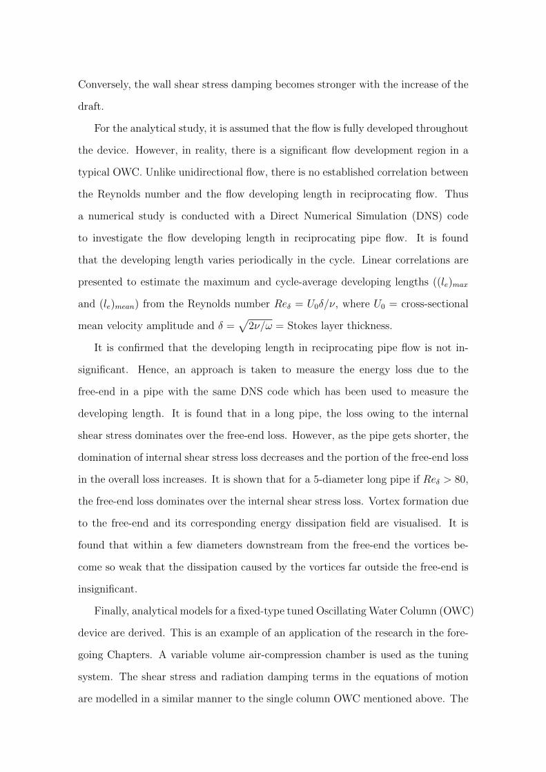
4.1 Schematic diagram of the geometry. . . . . . . . . . . . . . . . . . . . 60

4.2 Comparison between theoretical results (•) and simulation results (—

) of the velocity profiles in fully developed flow for (a) α′ = 4α2 = 50,

A0 = 3; (b) α′ = 400, A0 = 3. . . . . . . . . . . . . . . . . . . . . . . 61

4.3 Time history of the centreline velocity (uc) at the pipe entrance (◦)

and at the fully developed region (•) for α′ = 400 and A0 = 3. . . . . 62

4.4 Evolution of velocity profile along the pipe, at different phases of the

cycle for α′ = 400 and A0 = 3. . . . . . . . . . . . . . . . . . . . . . 63

4.5 Contours of (a) ∂u/∂r|w and (b) uc for α′ = 400 and A0 = 3, as a

function of the distance from the entrance (x) and the phase variation

φ; the symbols (•) show the location where (∂u/∂r|w)∞− ∂u/∂r|w =

0.01 and (uc)∞ − uc = 0.01 on the corresponding plots. . . . . . . . . 64

4.6 Contours of (a) ∂u/∂r|w and (b) uc for α′ = 400 and A0 = 3, as a

function of the distance from the entrance (x) and the phase variation

φ; the symbols (•) show the location where ∂(∂u/∂r|w)/∂x = 0.01 and

∂uc/∂x = 0.01 on the corresponding plots. . . . . . . . . . . . . . . . 65

vi

4.7 Maximum entrance length of the cycle, measured using (a) Method 1,

(b) Method 2; and the cycle-average entrance length measured using

(c) Method 1, (d) Method 2, as a function of α′, for A0 = 3. . . . . . 66

4.8 Maximum entrance length of the cycle measured using (a) Method 1,

(b) Method 2; and the cycle-average entrance length measured using

(c) Method 1, (d) Method 2, as a function of A0, for α′ = 400. . . . . 67

4.9 Maximum entrance length to diameter ratio as a function of α′ at

different A0. . . . . . . . . . . . . . . . . . . . . . . . . . . . . . . . . 68

4.10 Maximum entrance length to diameter ratio as a function of A0 for

α′ = 50, × ; α′ = 100, • ; α′ = 200, + ; and α′ = 400,

◦ . . . . . . . . . . . . . . . . . . . . . . . . . . . . . . . . . . . . 69

4.11 Maximum entrance length to Stokes-layer thickness ratio as a function

of Reδ for the range α′ from 100 to 400 and A0 from 1 to 9. The

straight line represents the correlation (le)max/δ = 1.37Reδ + 5.3. . . . 70

4.12 Cycle-average entrance length to diameter ratio as a function of α′ at

different A0. . . . . . . . . . . . . . . . . . . . . . . . . . . . . . . . . 71

4.13 Cycle-average entrance length to diameter ratio as a function of A0

for α′ = 50, × ; α′ = 100, • ; α′ = 200, + ; and α′ = 400,

◦ . . . . . . . . . . . . . . . . . . . . . . . . . . . . . . . . . . . . 71

4.14 Cycle-average entrance length to Stokes-layer thickness ratio as a

function of Reδ for the range α′ from 200 to 400 and A0 from 1 to 9.

The straight line represents the correlation (le)mean/δ = 0.82Reδ + 2.16. 72

5.1 Flow at the free-ends of a protruded pipe. . . . . . . . . . . . . . . . 75

5.2 Schematic diagram of the geometry. . . . . . . . . . . . . . . . . . . . 80

5.3 Control volume to investigate the free-end loss. . . . . . . . . . . . . 80

5.4 Comparison of cycle-average domain dissipation ˙Eew, computed by

the left side (◦) and right side (•) of equation (5.14); (a) as a function

of α′= 4α2, and (b) as a function of A0. . . . . . . . . . . . . . . . . . 82

vii

5.5 Comparison between theoretical results (◦) and simulation results (•)

of (a) wall friction coefficient Cf and (b) domain energy dissipation

˙Eew, as a function of α′ = 4α2 for A0 = 3. . . . . . . . . . . . . . . . 84

5.6 Cycle-average energy dissipation in the entire domain, ˙Eew; (a) as a

function of α′, (b) as a function of A0, (c) as a function of 1/(A0α′)

and (d) as a function of 1/(A0α′0.75). The straight dashed line in (d)

represents the correlation ˙Eew = 291.05/(A0α′0.75) + 0.035. . . . . . . 85

5.7 Cycle-average energy dissipation inside the pipe due to shear stress

assuming fully developed flow, ˙Ew; (a) as a function of α′, (b) as a

function of A0, (c) as a function of 1/(A0α′) and (d) as a function

of 1/(A0α′0.75). (e) The percentage contribution of ˙Ew in ˙Eew as a

function of 1/(A0α′0.5). The straight dashed line in (d) represents the

correlation ˙Ew = 276.15/(A0α′0.75) + 0.02. . . . . . . . . . . . . . . . 87

5.8 Cycle-average energy dissipation due to the free-end, ˙Ee; (a) as a

function of α′, (b) as a function of A0, (c) as a function of 1/(A0α′),

(d) as a function of 1/(A0.330 α′) and (e) as a function of 1/(A0.33

0 α′) for

A0 > 1. (f ) The percentage contribution of ˙Ee in ˙Eew as a function

of 1/(A0α′0.5). The dashed line in (d) represents the correlation ˙Ee =

1/[1 + 1.16(A0.330 α′)0.33]. . . . . . . . . . . . . . . . . . . . . . . . . . 88

5.9 Cycle-average energy dissipation outside the pipe due to the free-end,

˙Eeo; (a) as a function of α′, (b) as a function of A0, (c) as a function

of 1/(A0α′) and (d) as a function of 1/(A0.33

0 α′). (e) The percentage

contribution of Eeo in ˙Eew as a function of 1/(A0α′0.33). The dashed

line in (d) represents the correlation ˙Eeo = 1/[1 + 0.74(A0.330 α′)0.45]. . 90

5.10 Contours of vorticity (left) and energy dissipation (right) at the free-

end, for α′ = 400 and A0 = 3, at various oscillation phases φ. Red and

blue colours on the vorticity contour represent positive and negative

vortices respectively. . . . . . . . . . . . . . . . . . . . . . . . . . . . 92

viii

5.11 Comparison between the contribution of dissipations from the wall

shear stress (assuming fully developed flow) ˙Ew and from the free-

end ˙Ee to the overall domain dissipation ˙Eew as a function of 1/Reδ

for different pipe lengths. . . . . . . . . . . . . . . . . . . . . . . . . . 94

5.12 Cycle-average total dissipation ˙Eew in a domain with a 2.3-diameter

long pipe (to match the length of the pipe of [12]), as a function of

A0 at low α′ (from simulation) and at high α′ (from experiment [12]). 95

6.1 OWC with an air-compression chamber; (a) Schematic diagram, (b)

Water (green) and air (grey) zones in the device. . . . . . . . . . . . . 98

6.2 Dimensions of the OWC device. . . . . . . . . . . . . . . . . . . . . . 101

6.3 Average dimensionless power against dimensionless parameter Kh for

different damping : —, radiation (βrd); —, radiation and turbulent

(βrd + βtb) and —, radiation, turbulent and free-end (βrd + βtb + βfe). 110

ix

Chapter 1

Introduction

The traditional methods of energy production from the nuclear and fossil fuel have

become a serious threat to the environment due to their contributions in global

warming, air pollution, acid precipitation, ozone depletion, forest destruction, and

emission of radioactive substances [13]. Additionally, these energy resources are

limited in nature. Thus the global trend is shifting towards safer, cleaner and

renewable energy generation schemes. The contribution of hydro-power, solar and

wind energy to the world energy demand is well appreciated. However, there is

another very promising and vast renewable energy resource which has been remained

unharnessed; that is ocean wave energy. The wave energy in the ocean did not get

much attention until the oil-crisis of 1973 [14]. After that incidence, the demand

for harnessing new renewable energy sources has been encouraging governments and

industries to focus on the ocean wave energy. One of the most attractive features of

the ocean waves is that they have very high energy flux, in fact the highest among

the other renewable sources [15]. Another attractive characteristic of the ocean wave

is that once it is created, it can travel very long distances with very low energy loss.

Furthermore, unlike the solar or wind energy sources, the energy that is carried by

the ocean waves is nearly independent of the local weather. It is estimated that wave

energy has a lower variability with respect to wind energy (for example it is only

one-third of the variability of wind energy in Australia [16]). Another estimation

shows that the total wave energy that is available in the world’s ocean is of the same

1

order of magnitude of the world’s total electricity consumption [17]. Although it is

only possible to exploit 10− 20% of this energy resource [18], the potential of ocean

wave energy to contribute to human energy demand is clearly very significant.

Technologies to extract energy from the renewable energy sources like the sun,

wind and hydro head are well established and have been using successfully for the

past few decades; in the case of wind power, for centuries; and for hydroelectricity, a

century. However, to extract energy from ocean waves many different types of Wave

Energy Converters (WECs) have been proposed. Although some WECs reached

the prototype level and are successfully operating in different coastal areas of the

world, significant development is still required to make the WECs competitive with

other renewable energy converters [14]. More than a thousand patents for WECs

had been registered in Japan, North America and Europe by 1980 [19], and new

ideas are coming up every year. Recent reviews on WECs found that around one

hundred development projects are going on at different places in the world [14].

WECs are generally classified based on their location (i.e. offshore or onshore),

size (i.e. point absorber or large absorber) and working principle. Based on the

working principle WECs were categorised in three types; Oscillating Water Columns

(OWCs), Oscillating Bodies and Overtopping devices [14].

Among the different types of WECs, the OWC is considered one of the most

promising technologies owing to its ease of construction, few moving parts, easy

(a) Prototype OWC [20]. (b) Schematic of the OWC [21].

Figure 1.1. Fixed structure OWC.

2

(a) Prototype OWC [22]. (b) Schematic of the OWC [23].

Figure 1.2. Floating type OWC.

maintenance and high reliability [2]. There are two types of OWCs; the fixed struc-

ture OWCs (Figure 1.1), usually located on the shoreline or near shore, and the

floating type OWCs (Figure 1.2). The fixed structure OWCs are also known as

the first generation devices. OWCs are basically comprised of a partly submerged

structure which is open below the water surface, is called the collector chamber, an

air chamber above the water surface and the Power Take Off (PTO) mechanism as

shown in Figure 1.1(b) and 1.2(b). The air-water interface in the collector chamber

oscillates owing to the rising and falling of the waves in the sea. As the air-water in-

terface moves up, the air in the air-chamber is pushed out through a turbine which

is mounted at the top of the air-chamber. As the interface moves down, the air

from the outside is pulled in through the turbine. The axial-flow Wells turbine and

the impulse turbine with guided vanes are most commonly used turbines in OWC

plants. These turbines are designed in such a way that they rotate in one direction

regardless of the direction of the air flow.

An OWC can extract the maximum amount of power when the device natural

frequency coincides with the incoming wave frequency; i.e. the system resonates.

The device could extract enormous amounts of energy at resonance, unless the

damping is significant. Therefore, the damping factors in the device play a major

role in controlling the overall efficiency of the system. In principle, the optimum

3

power is extracted by a fixed-type OWC (where the duct is considered fixed relative

to the ocean floor) operating with linear dynamics when it resonates and the rate

of useful energy absorption is equal to the rate of damping [24].

The basic working principle of an OWC is like a forced mass-spring-damping

system, where the water column represents the mass, and the body force on it

(due to gravity) plays the role of the spring restoring force. The damping, which

is the primary focus of this study, consists of different terms representing different

mechanisms of energy loss as the OWC operates.

These mechanisms include the wall shear stress. Boundary layers introduce vis-

cous and turbulent dissipation causing a loss of energy. A second mechanism is

radiative waves, in which pressure fluctuation in the air chamber causes a secondary

wave to radiate away some energy. The third mechanism is the PTO system. A

significant amount of damping comes from the PTO system, which is, in general,

a turbine-generator arrangement and this, of course, represents the useful power

extracted from waves. Finally, vortex formation at the submerged end of the pipe

dissipates a significant amount of energy. Furthermore, if the device is sufficiently

wide, another mechanism is sloshing of the internal air-water interface, which also

causes damping.

The impact of these different damping factors on the overall power output has

not been rigorously studied. The focus of much analysis has been radiative damp-

ing, since this can be analysed by potential-flow theory. Theories on calculating

the radiation damping and hence estimating the efficiency of an OWC have been

thoroughly derived in [25, 26]. However, overall, true damping is one of the most im-

portant design prerequisites, required to estimate the total amount of energy loss.

Laboratory experiments have reported on energy losses in scale models of actual

devices [27]. Very few theoretical studies have incorporated the dissipation from

shear into models [12, 28]. Numerical studies on the internal flow dynamics of an

OWC using standard computational fluid dynamics packages which use turbulence

models, e.g. k-ε etc., may yield overall performance results, however it is not clear

4

that such turbulence models will perform with fidelity for high Reynolds number

reciprocating flow, for which there is very few data available (e.g. [29]) to validate

the models.

In Chapter 3 of the present work, a fluid-dynamical approach is taken to derive

the mass-spring-damping model of an OWC from the Navier-Stokes equations. In

order to examine the essential physics without undue complexity, a simple fixed-type

cylindrical OWC is considered. The radiation damping derived in [1] is adapted to

the present model after transforming to a rigid-body model as explained in [30].

Air in the air-chamber is considered compressible, though it is assumed that the air

pressure maintains a linear relationship with the mass flow rate through the turbine

(as in a Wells turbine model [31]).

The first-order flow created inside the OWC by ocean waves is reciprocating, i.e.

it is periodic and completely reverses direction. A novel contribution of the present

work is the inclusion of the resulting reciprocating shear stress, modelled based on

the theory developed in [32] and the Blasius correlation for steady turbulent flows in

smooth pipes, as justified in [9]. Flow inside the device is assumed fully-developed to

neglect the effect of the developing region and vortices at the entrance. A comparison

of overall power output is presented for different wall shear stress models.

Though the flow is considered fully-developed while deriving the analytical mod-

els of a simple OWC, in reality, there is developing length at the free-end of the

OWC. Unlike the unidirectional flow, there is no well established relationship be-

tween the Reynolds number and the developing length in reciprocating flow. Thus,

in Chapter 4 a numerical approach is taken to measure the developing length in

the reciprocating pipe flow. This is also a novel contribution of the present work.

A pipe with free-ends exiting to reservoirs is used for the investigation. The flow

rate at the inlets is driven sinusoidally with time, and equal and opposite at each

end. A structured mesh is used to run the simulations. The DNS code used in

this study uses a nodal-based spectral-element method to solve the incompressible

Navier-Stokes equations. It is assumed that the flow is axisymmetric throughout

5

the flow domain. Both the maximum developing length in a cycle and the cycle

averaged developing length are presented as a function of Reynolds number.

Once it is confirmed that the developing length in reciprocating pipe flow is not

negligible, the rate of energy loss within the developing region and the rate of loss

outside the pipe due to the free-end are measured and presented in Chapter 5. The

wall shear stress and free-end losses are measured separately in reciprocating pipe

flow to make a comparison between them. The DNS code which has been used in

Chapter 4 to measure the developing length, is used in this Chapter to measure the

energy loss. While measuring the free-end loss, first the energy dissipation due to

the wall shear stress inside the pipe is calculated assuming that the flow is fully-

developed through out the pipe. Then the wall shear stress loss is subtracted from

the entire flow domain loss. This enables incorporation of the measured free-end

loss into the analytical model in Chapter 3, since the analytical modelling has also

been done assuming a fully-developed flow in the pipe.

Finally, the preceding results are applied to a practical example of a new design.

The analytical models for a fixed-type tuned Oscillating Water Column (OWC) de-

vice are derived, incorporating the losses due to shear stress (viscous and turbulent),

radiation wave and the free-end in Chapter 6. It is expected that the OWCs will

resonate at the incident wave frequencies to ensure the maximum amount of power

extraction. This is possible when the natural frequency of the device coincides with

the incident wave frequency. However, the wave frequency varies within a significant

range. Therefore, to maintain the resonance condition, it may be beneficial to have a

tuning mechanism which will adjust the natural frequency of the device to the wave

frequency. Several tuning mechanisms have been proposed for fixed type OWCs,

such as a variable-volume air compression chamber in a seawater pump [28] and the

U-OWC device [33]. The present work incorporates the idea of a variable volume

air-compression chamber as the tuning system in an OWC. A comparison between

the power output before and after the inclusion of free-end damping is presented.

The aim of the present work is to incorporate all the most significant forms of

6

dissipation in an OWC into a simple, yet rigorous model that is useful for design.

One of the novel contributions of the present work is the inclusion of the resulting

reciprocating shear stress, modelled based on the theory developed in [32] and the

Blasius correlation for steady turbulent flows in smooth pipes, as justified in [9].

Other novel contributions are the estimation of the developing length in reciprocating

pipe flow, and then measurement of the energy loss in the development region, along

with the loss outside the pipe due to vortex formation.

7

Chapter 2

Literature Review

In this chapter, significant research that contributed and has potential to contribute

to developing the oscillating water column (OWC) are highlighted. Relevant lit-

erature are presented in three sections. In the first part, the history of develop-

ing prototype OWCs is given. Numerous works have been done on the analytical

modelling of OWCs; they are reported in the second part. This second part is fur-

ther divided into two subsections. In the first subsection, literature on analytical

modelling to evaluate the performance of OWCs are presented, such as the power

absorption efficiency from waves and power conversion efficiency. In the second sub-

section, different works on the tuning mechanism of OWCs are presented. Most

of the theoretical modelling of OWCs has been done by assuming an irrotational

flow inside the device. However, this assumption is valid when the viscous shear

stress is considered negligible. As discussed in Chapter 1, one of the main aims of

the present work is to include the viscous and turbulent shear stress in an analyt-

ical model of a fixed type near-shore OWC and to study the effect of these shear

stresses on the power extraction. Since the flow inside the device is reciprocating

(oscillatory flow with zero mean), the existing well-established shear stress model

for steady flow is not compatible with the equations of motion of OWCs. Therefore

literature on reciprocating flow are studied to understand the flow characteristics

and the contribution of viscous and turbulent shear stresses to energy dissipation.

These literature on bounded reciprocating flow are presented in the third part of

8

this chapter.

2.1 Background of OWCs

The earliest patent on wave energy converters was filed in 1799 in France, when

Pierre Girard and his son proposed a device to harness the power from waves [34].

The device was proposed to utilise the bobbing of moored ships to run heavy ma-

chinery ashore via a plank and fulcrum mechanism. Though the device was never

constructed, it inspired the engineers of the following generations to work in this

field. After almost a century, J. M. Courtney from New York patented a device,

known as the Whistling Buoy (Figure 2.1) which is considered as the earliest ap-

plication of an OWC [2]. It was an audible warning device, used for a navigation

aid.

Until 1940, numerous patents on wave energy converters had been registered.

Very few of them were successful in producing the expected amount of power. The

first electricity-generating OWC was built in the 1940s by Yoshio Masuda in Japan.

He developed a floating OWC by installing an impulse air turbine on a navigation

buoy. This buoy was sited in Osaka Bay and the generated electricity was using to

Figure 2.1. Courtney’s Whistling Buoy [2].

9

power navigation lights. From 1965, this device was commercialized in Japan and

later in the USA [14]. In 1976, Masuda led a team from the International Energy

Agency to test the performance of several OWC units mounted on a floating barge,

named Kaimei [2]. The dimension of that 800 tonne barge was 80×12 m and it was

placed at the coast of Yura, Tsuruoka City, Japan. These OWC units were equipped

with different air turbines such as the Wells turbine, McCormick turbine and some

other turbines with rectification valves. Eight OWC units were mounted on that

barge and each of them had the capacity of generating 125 kW power. This testing

program was sponsored by Japan, UK, Canada, Ireland and USA. It is possible

that the lack of sufficient theoretical knowledge on the wave energy absorption at

that early stage of OWC development caused the project not to be as successful as

expected [14].

Since 1975, several countries in Europe such as the UK, Norway, Portugal and

Ireland started conducting research on wave energy extraction devices [14]. As a

result, in 1985, two shoreline prototypes of 350 kW and 500 kW capacity were de-

ployed near Bergen, Norway. Later in 1991, a small 75 kW OWC was deployed at

Islay island, Scotland [35]. Apart from these physical developments, the noticeable

advancement in Europe in the following few years was the development of theoreti-

cal knowledge on wave absorption techniques which will be detailed in section 2.2.

Meanwhile in Japan, a 60 kW OWC was integrated into a breakwater [36], and in

India, a bottom-standing 125 kW OWC was constructed [14]. The largest OWC

(bottom standing) device with a capacity of 2 MW, named OSPREY, was deployed

near the Scottish coast in 1995. However, it was destroyed by the sea shortly after

the installation [14]. In July 1998, a floating-type OWC of 110 kW, named The

Mighty Whale, was built by Japan Marine Science [37]. The first prototype OWC

in Portugal with a capacity of 400 kW was built in 1999 at the island of Pico [38];

this is a shore-base OWC. In the following year, another shore-based OWC of 75

kW, named LIMPET was deployed at the Islay Island, Scotland [2]. At Port Kem-

bla, Australia, a bottom standing OWC plant of 1.5 MW with a parabolic-shaped

10

collector was deployed by the Oceanlinx (formarly Energytech) in 2005 [39]. The

Backward Bent Duct Buoy (BBDB) type OWC, invented by Masuda, have been

used in Japan and China to power about a thousand navigation buoys [40]. In

2010, Oceanlinx built a floating-type OWC which was a one-third scale of the 2.5

MW full-scale device [22]. A quarter scale BBDB converter by Ocean Energy was

installed for sea trials at Spiddal in Galway, Ireland in 2011 [41]. In the same year,

a breakwater OWC started to operate at Mutriku Basque Country, Spain; 16 sets

of Wells turbines with a capacity of 18.5 kW each were installed in that plant [42].

Among the most recent OWCs, Oceanlinx built a 1 MW fixed-type OWC named

the greenWAVE at Port Adelaide, Australia in 2014 [22]. However, the plant was

not successfully deployed because of an accident which occurred while towing the

OWC from the construction site. Additionally, a 500 kW bottom-standing OWC

with a dimension of 37× 31.2 m was deployed at Jeju Island, South Korea in 2015

[43]. At Civitavecchia harbour in Italy a breakwater OWC plant was completed in

2016. This plant is comprised of 17 caissons containing 124 U-OWCs. This plant,

like all others, was designed such a way that the natural frequencies of the OWCs

can be tuned with the incident wave frequency so that the OWCs resonate [33, 44].

2.2 Theoretical modelling of OWCs

Literature on the theoretical modelling of OWCs are presented in two subsections.

The first part highlights the works that dealt with the performance evaluation of

general OWCs; such as the efficiency of energy absorption from the incident waves

and the overall efficiency of energy extraction. As noted before, the maximum power

output from OWCs is achieved when the natural frequency of the device coincides

with the incident wave frequency, i.e., when the device resonates. Since the wave

frequency varies within a wide range, it may be beneficial to have a tuning system

which can adjust the device natural frequency with the incident wave frequency.

There are few analytical works on tuned OWCs are available in the literature. These

are presented in the second part of this section.

11

2.2.1 Performance evaluation of OWCs

The mathematical development of OWC theory began in 1970s, specially after the

oil crisis in 1973. The first theoretical expression to estimate the efficiency of a fixed-

type OWC device was derived in [45]. It gives an analytical solution to evaluate the

energy absorption efficiency of a simple OWC device. The device was assumed to

be comprised of a float which oscillates with the water column, a spring-dashpot

system that is connected to the float, and two closely-spaced vertical parallel plates

or a narrow tube which encompass the whole system. In that model, linearized

water wave theory was used. The problem was simplified by assuming the float

weightless and the spring with zero stiffness. The closely spaced plates or narrow

tube assumption made it possible to adapt the matched asymptotic expansions

method which was derived in [46]. The analytical solution can be used without

any difficulty for the two fully submerged plates or, in three dimensions, for a fully

submerged tube. It has been shown that it is possible to absorb a maximum of 50%

of the incident wave energy if the two parallel plates are of equal length. However,

with an extended version of the two dimensional model, it can be shown that a

device with two plates of unequal length can extract more than 50% of the incident

wave energy. It has also been shown in [46] that for the three-dimensional case, it is

theoretically possible to capture the energy in a wave whose crest length (the length

of a wave along its crest) is greater than the tube diameter.

An upgraded version of the above-mentioned theory has been derived in [25]. It

explains an OWC system as one driven by an uniform oscillatory surface pressure.

This theory considers a device that is fixed, open at the bottom-end, closed at the

top-end and intersecting the free water surface. The device has several air chambers

which trap a volume of air above each of the internal free surfaces. The general

working principle of the device is as follows. The wave passes through it, and the

free surface inside the device rises and falls which initiates a reciprocating movement

of the volume of air through a constriction, which is an air turbine connected to an

electricity generator. To simplify the model in [25], a simple orifice plate was used

12

in exchange of the turbine-generator arrangement. The hydrodynamics of the OWC

has been modelled based on the simple assumption that the water column oscillates

as a rigid body. To incorporate the theory into the model, a weightless piston of

known damping and added mass have been assumed in place of the free surface.

A similar approach but neglecting the spatial variation in the internal free sur-

face caused by the surface pressure was given in [45] (mentioned earlier). In [25],

a more accurate and simpler theory was presented for such devices which take the

surface pressure and the consequent spatial variation of the internal free surface into

consideration. Linearized water-wave theory was used. The compressibility of air

was neglected which allowed consideration of a linear relationship between the pres-

sure drop across the turbine and the volume flow rate through the turbine. General

expressions for the mean power absorbed by an arbitrary pressure distribution sys-

tem were derived in terms of an admittance matrix. It related the overall volume

flux Q∗ to the pressure applied to the system p∗a, the induced volume flux due to

the incident1 and scattered2 potential Q∗s, and the (assumed linear) pressure-volume

flux characteristics across the turbine (PTO system). A further explanation of these

parameters is given in Appendix B.1.

For perfect impedance matching3, it has been shown in [25] that solving the

linear wave-diffraction problem is sufficient to estimate the absorbed mean power.

However, in the case of imperfect matching, for a single pressure distribution in ei-

ther two or three dimensions, synchronisation between the pressure distribution and

the incident wavelength is required to achieve resonance. Comparing the resonant

condition of the OWC device with the equivalent rigid-body wave-energy devices, it

has been shown in [25] that the devices operating on the surface-pressure principle

can be described by the rigid body models and the results would not vary much.

In [26], a two-dimensional analysis based on the linear surface-wave theory was

1The incident wave potential is the velocity potential due to the incident wave when there isno PTO system in the device.

2The scattered wave potential is the velocity potential due to the wave that is diffracted by thedevice.

3Perfect Impedance matching: when the applied pressure p∗a is a linear combination of thevolume flux induced by the incident and scattered waves Q∗s [25].

13

derived. The combined effects of finite water depth, air compressibility and the tur-

bine characteristic were studied. A phase difference between the pressure and the

flow rate through the turbine was considered while modelling the turbine effect. For

the sake of simpler analytical expressions, the wave diffraction due to the immersed

part of the structure was ignored. Additionally, the instantaneous mass-flow rate

through the air turbine or equivalent device which produces the work from the oscil-

lation of the air in the chamber was assumed to be a known function of the pressure

difference. Both linear and nonlinear effects of the power take-off (PTO) system

were considered while modelling the OWC to make the analysis more comprehen-

sive. For the linear case, the springlike effect of air compressibility was assumed of

constant stiffness and the mass-flow rate through the air turbine was considered pro-

portional to the pressure difference across it. For the nonlinear analysis, numerical

calculations were done based on Brown’s method [47]. The linearized approximation

and the nonlinear isentropic relation between the density and the pressure were used

to compute the device efficiency. It was found that there is no significant difference

of efficiency calculated by these models except for the cases with large wave ampli-

tudes. In case of the nonlinear PTO system, the mass flow rate has been considered

to be proportional to the square root of the pressure difference.

It has also been shown in [26] that the air compressibility has a significant role

on the performance of the OWC if the air chamber height is several metres long.

Moreover, it was determined that the compression and expansion processes of air

deviate from the isentropic process due to the viscous loss in the flow through

the turbine. It was noticed that the size of the chamber and the turbine can be

reduced substantially until the system is optimally efficient. Further reduction of

these parameters causes a deficiency in overall turbine performance due to the joint

effect of viscous loss and increasing phase difference. It was stated that almost 100%

efficiency may be achieved even for a strongly nonlinear PTO system if the system

is tuned to the wavelength and to the wave amplitude.

A general theory was derived for a composite system of both oscillating bodies

14

and oscillating pressure distributions in [48]. This model is well suited to the deriva-

tion of dynamics of floating-type OWCs, since these OWCs are comprised of both

an oscillating body (OWC structure) and an oscillating pressure distribution (pres-

sure distribution inside the device). Like the above-mentioned works, linear water

wave theory has been used for the derivation. The coupling was derived between

the oscillators and represented in the form of a matrix equation which is comprised

of (analogously to electric circuit theory) the radiation admittance matrix for the

pressure distributions, the radiation impedance matrix for the oscillating bodies,

and a radiation coupling matrix between the bodies and the pressure distributions.

A formula was derived to relate the added mass and the difference between the

kinetic and potential energy of the near-field region.

In [49], hydrodynamic coefficients of a fixed-type OWC operating in a finite

water depth were expressed in terms of integral quantities of functions using the

linear water wave theory. These functions are proportional to the fluid velocity

inside the device. A Galerkin method was used to calculate the hydrodynamic

coefficients from the governing integral equations.

A linear analytical model of OWCs including the loss due to viscous shear stress

was presented in [30]. A derivation to transform the pressure distribution model to a

rigid body model was presented. Loss due to viscous shear stress was first introduced

into the rigid body model and then the transformation was used to include viscous

loss into the pressure distribution model.

In [1], an approach similar to [49] was taken to calculate the hydrodynamic

coefficients of fixed-type cylindrical OWCs. Like [49], the theory of pressure distri-

butions was used, and a Galerkin method was used to compute the hydrodynamic

coefficients; however the main difference is that the two dimensional model of [49]

has been extended to three dimensions in [1]. The total induced volume flux across

the internal free surface was considered to be the sum of induced volume fluxes due

to the scattered and radiated4 waves. The radiation volume flux was further split

4The radiated wave is the wave that radiates away from the device due to the pressure fluctuationin the air chamber when there is no incident wave.

15

into two terms which are composed of coefficients. These coefficients are analogous

to the added mass and radiation damping coefficients in the rigid-body model as

explained in [48]. These added mass and radiation damping coefficients have been

incorporated in the present study while modelling an OWC analytically in Chapter

3. It was shown that the narrower the device, the closer the pressure distribution

model is to the rigid body model.

An analytical model for the power extraction from an OWC at the tip of a break-

water was presented in [50]. The integral equations were solved for the radiation and

scattering problems in a cylindrical OWC with an open bottom. An exact solution

of the diffraction problems due to the OWC and the breakwater was derived. The

power take-off was modelled by considering the air compressibility in air chamber.

It was found that the angle of incidence affects the flow field outside the device,

however it does not affect the power extraction.

All the above mentioned works used the linear wave theory to evaluate the per-

formance of OWCs. In linear wave theory it is assumed that the flow is irrotational.

However in OWCs, there is rotational flow due to the presence of the boundary

layer inside the device and due to the free-end. Thus an analytical model is required

which will include the effects of boundary layers and the free-end. Though [30]

showed a procedure to incorporate the viscous loss into the linear OWC model, no

specific modelling of the viscous term was presented which could be used to estimate

the contribution of the viscosity in the overall performance of OWCs. Therefore,

an approach is taken in the present study to incorporate both the viscous and the

free-end effects into the linear wave modelling.

2.2.2 Tuning mechanisms of OWC devices

As mentioned in Chapter 1, it is possible to extract the maximum amount of energy

is possible to extract when OWCs operate at resonance i.e. the natural frequency

of the device coincides with the wave frequency. At resonance, oscillations increase

linearly in time until damping inhibits further growth. Most of the OWCs are

16

designed to meet the resonance condition. Another way to improve the performance

of OWCs is to synchronise the oscillation of the water-column inside the device with

the oscillation of the incident wave in such a way that the phase difference between

these oscillations should be minimum. This method is known as the phase-locking

mechanism.

To achieve either the resonance or the phase-locking condition, a tuning mecha-

nism is required in the device. The findings of the present work are to be illustrated

by applying them to the derivation of the governing equations for a tuned OWC,

which is presented in Chapter 6. Thus the literature on different tuned OWCs have

been studied and presented in this section.

A tuning mechanism of an OWC sea-water pump was presented in [3, 28]. The

sea-water pump is comprised of a resonant duct, a variable volume air-compression

chamber and an exhaust duct as shown in Figure 2.2. The air in the air-compression

chamber works like a spring. The variable-volume function of the chamber can

be used to tune the device natural frequency with the incident wave frequency

by adjusting the stiffness of the air. As a wave passes the device, it induces a

pressure at the mouth of the resonant duct which causes the flow to oscillate inside.

Consequently, the water in the exhaust duct is channelled to the receiving body.

The equations of motion of the water columns were derived from the time-dependent

Bernoulli’s equation. Damping terms due to the viscosity, vortex formation and wave

Air compression chamber

Resonant ductExhaust duct

Adjacent

compartment

Figure 2.2. Schematic diagram of the seawater pump [3].

17

radiation were incorporated into the equations of motion respectively from [51], [11]

and [12]. The equations were linearized by assuming that there is no sloshing at

the free-surface inside the device. The system has two degrees of freedom due to

the presence of two oscillating masses which oscillate in two modes; firstly, both the

water-columns along with the air in the air-compression chamber oscillate as a single

body, and secondly the water-columns oscillate against each other by compressing

and expanding the air. Thus two natural frequencies were obtained.

In [52], experiments were conducted in a wave tank with a 1 : 20 scale model

of the above-mentioned sea-water pump. A tuning algorithm was developed to

estimate the optimal volume of air in the air-compression chamber for a range of wave

period, amplitude and tidal elevation. Experiments and numerical simulations were

conducted for different polychromatic wave spectra. Results from the experiment

and numerical simulation were used to develop a tuning criterion that optimises the

system performance. No difference between the monochromatic and polychromatic

waves was observed. It was found that the pumping was optimum when the system

was tuned to the waves of lower frequencies.

A dynamic tuning mechanism of the OWC sea-water pump was presented in [4].

Generally, in a dynamic tuning system, one of the influential parameters (e.g. in

the sea-water pump, the mass of the water column and the stiffness of air in the

air-compression chamber) is varied periodically. The resultant resonance is known

as the parametric resonance. In parametric resonance, the oscillations increase ex-

ponentially with time. The main advantage of the parametric resonance over the

general resonance is once the system reaches the maximum amplitude, the oscilla-

tion does not modulate even if the system is not exactly tuned. In [4], the stiffness of

air in the air-compression chamber was varied periodically with the aid of a variable

volume air-compression chamber to achieve the parametric resonance. Figure 2.3

shows the set-up that was used to investigate the parametric resonance. In that

set-up, there were two air chambers; the main air chamber and the adjacent air

chamber. The extra volume of air in the adjacent chamber was used to increase

18

x

Tank

L

Compression chamber

V0

V∆

Equilibrium level

ValvePiston

Figure 2.3. Possible implementation of a parametric excitation of an OWC. Thevolume of the air-compression chamber is changed by the action of the piston andthe valve [4].

and decrease the overall volume of air by opening and closing the valve and conse-

quently softening and hardening the air-spring restoring force. A piston was used

to adjust the equilibrium position of the water-column surface in such a way that it

compensates for any difference due to the opening or closing of the valve.

In [5], a modified version of the conventional breakwater OWC, named the U-

OWC, was presented (Figure 2.4(b)). In the U-OWC, an additional water column

(a) (b)

Figure 2.4. Breakwater embodying OWC; (a) single column OWC, (b) U-OWC[5].

19

is introduced by adding an extra vertical duct. Though it is not an exact tuning

system, the introduction of an extra column improves the performance of the device.

Two reasons were mentioned for the performance improvement; firstly, owing to

the increase in water column length, the natural frequency of the device decreases

and hence the difference between the incident wave frequency and device natural

frequency also decreases (i.e. the system gets closer to the resonance condition).

Secondly, the pressure at the U-OWC entrance fluctuates with higher amplitude than

at the entrance of a conventional single column OWC since the entrance can now be

close to the surface, where the pressure induced by waves is maximal. Because of

these reasons, the U-OWC showed a better performance with all types of waves, i.e.

swell, small and large wind waves. A performance comparison between the U-OWC

and the conventional OWC was performed based on the theory presented in [53].

A case study on installing the U-OWC at two sites along the Italian coast (the

port of Civitavecchia and the port of Pantelleria) was presented in [54]. An ad-

vanced Wave Model (WAM) along with a numerical algorithm which determines

the shoaling-reflection effects on the wave energy propagation was used to conduct

the study. It was shown that the plant can absorb around 75% of the incident wave

power.

The present study deals with a cylindrical OWC (Chapter 3). Thus, while in-

troducing a tuning system to the device (Chapter 6), it is found that the variable

volume air-compression chamber concept of [3] would be the best suited option for

the present study.

2.3 Reciprocating pipe flow

As mentioned earlier, the flow inside the OWC is reciprocating (oscillatory flow with

zero mean). Very few works were done on the viscous reciprocating flow dynamics

in OWCs. However, some studies were conducted on wall-bounded oscillatory flow

due to its presence in many biological and industrial processes like blood flow in the

cardiovascular system, water hammer and surging in pipe flows and fluid-control

20

systems, wave-height damping and sediment movement by water waves and so on

[55]. This section of the literature review focuses on the works (analytical, exper-

imental and numerical) done on the reciprocating pipe flow investigating the flow

characteristics, transition from laminar to turbulent flow, flow developing length,

and energy loss due to the shear stress and entrance effects.

As mentioned in Chapter 1, one of the prime goals of the present work is to build

up a numerical set-up which would enable investigation of different flow character-

istics in reciprocating pipe flow, which might be difficult to conduct experimentally.

This set-up is further used to estimate energy loss due to the shear stress and free-

end effect of the OWC “pipe”. These estimated losses are then incorporated as a

damping term into the equation of motion of the OWC. The literature are reported

in chronological order.

2.3.1 Flow characteristics and transition from laminar to

turbulent

A unique phenomenon in reciprocating flow is the “annular effect”, discovered by

Richardson & Tyler in 1921 [56]. They found that unlike in unidirectional flow, the

average velocity in reciprocating flow is maximum near the pipe wall. It was also

observed that a layer of laminar flow exists near the walls, though the main body

of the flow is turbulent.

A very useful non-dimensional parameter in oscillatory and pulsatile flow is the

Womersley number (α = 12D√ω/ν, where D is the diameter of the pipe, ω is the

oscillation frequency and ν is the kinematic viscosity), first introduced in [57] by

Womersley in 1955. In that work he derived an exact solution of the equation of

motion for reciprocating pipe flow.

Another remarkable theoretical work on reciprocating pipe flow is [32], done by

Uchida in 1956. The linearized incompressible Navier-Stokes equations were used to

derive an exact solution of reciprocating laminar flow superposed on a steady flow

in circular pipe. The non-linear Navier-Stokes equations were linearized assuming

21

parallel flow in the pipe. It was found that as the oscillation frequency increases,

the amplitude at the centre of the pipe diminishes and the phase difference between

the velocity and pressure gradient increases from 00 to 900. At higher frequency,

theoretical velocity profiles of reciprocating flow agree with the finding in [56], show-

ing that the maximum average velocity exists near the wall. Additionally, it was

shown that the cycle-averaged work done by the kinetic energy is zero. However,

the cycle-averaged energy dissipation due to internal friction is always finite.

For unidirectional pipe flow the critical Reynolds number (Re∗), at which the

flow enters into the transient regime from the laminar regime is around 2300. And

Re∗, for which the flow enters into the turbulent regime from the transient regime,

is around 4000. These values are universally accepted because of their repeated

appearance in numerous investigations since the original work of Reynolds in 1880.

However, for reciprocating flow the number of investigations into equivalent critical

transition points are very few. Therefore the critical Reynolds numbers in recipro-

cating pipe flow are still a matter of further study.

In 1966, Sergeev conducted an experiment on a reciprocating flow in a vertical

pipe with a bellows connected to it, as shown in Figure 2.5 [6]. Studies were done

Figure 2.5. Schematic of experimental set-up of [6], where 1. Test pipe; 2. bellows;3. structure; 4. strain gage; 5. crank mechanism.

to measure the values of the critical Reynolds number and the damping forces in

22

laminar and turbulent regimes. Two dimensionless numbers were used to define the

conditions of transition; the oscillatory Reynolds number, Reos = U0D/ν and the

Womersley number α = 12D√ω/ν where U0 is the amplitude of cross-sectional mean

velocity, D is the diameter of the pipe, ω is the oscillation frequency and ν is the

kinematic viscosity. Experiments were done for the range of 4×103 ≤ Reos ≤ 30×103

and 4 ≤ α ≤ 40. The critical Reynolds number, Re∗os was found to be proportional

to α with a proportionality constant of 700; i.e.,

Re∗os = 700α for 4 ≤ α ≤ 40. (2.1)

Partial turbulence was observed at lower values, α < 12, when the average fluid

velocity was changing its direction during the oscillation. However, at all values of

α, a disordered motion was noticed over a length of less than ten pipe diameters

from the inlet.

Experiments were conducted on the pipe flow for different length to diameter

(L/D) ratios. It was found that the damping due to entrance losses is very small.

It was also observed that the viscous damping increases very little with the increase

of Reos in the laminar regime. The friction coefficient in the turbulent regime (for

α = 19, Reos ≈ 15×103 and for α = 7, Reos ≈ 4×103) was found to be approximately

equal to that given by the Blasius correlation, f = 0.316Re−0.25.

Almost a decade later, in 1975, Merkli and Thomann performed an experimental

study on the transition in oscillatory flow [58]. Experiments were done within the

range 42 / α / 71. It was found that turbulence appears only in a certain portion

of the flow cycle and remains absent in the rest of the flow. It was also shown that

the critical Reynolds number is

Re∗os = 400α for 42 / α / 71. (2.2)

A detailed study of the velocity profile, flow stability, and consequently the transi-

tion points in reciprocating pipe flow was done by Hino in 1976 [7]. Experiments were

23

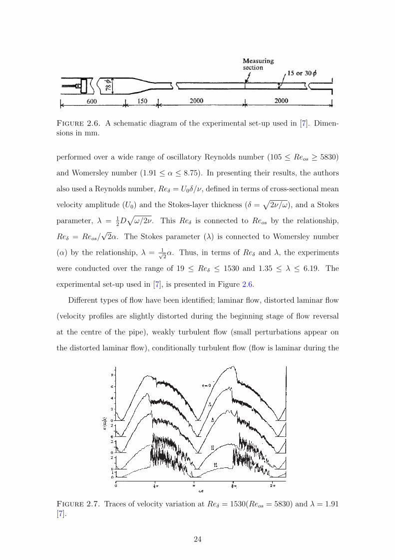
Figure 2.6. A schematic diagram of the experimental set-up used in [7]. Dimen-sions in mm.

performed over a wide range of oscillatory Reynolds number (105 ≤ Reos ≥ 5830)

and Womersley number (1.91 ≤ α ≤ 8.75). In presenting their results, the authors

also used a Reynolds number, Reδ = U0δ/ν, defined in terms of cross-sectional mean

velocity amplitude (U0) and the Stokes-layer thickness (δ =√

2ν/ω), and a Stokes

parameter, λ = 12D√ω/2ν. This Reδ is connected to Reos by the relationship,

Reδ = Reos/√

2α. The Stokes parameter (λ) is connected to Womersley number

(α) by the relationship, λ = 1√2α. Thus, in terms of Reδ and λ, the experiments

were conducted over the range of 19 ≤ Reδ ≤ 1530 and 1.35 ≤ λ ≤ 6.19. The

experimental set-up used in [7], is presented in Figure 2.6.

Different types of flow have been identified; laminar flow, distorted laminar flow

(velocity profiles are slightly distorted during the beginning stage of flow reversal

at the centre of the pipe), weakly turbulent flow (small perturbations appear on

the distorted laminar flow), conditionally turbulent flow (flow is laminar during the

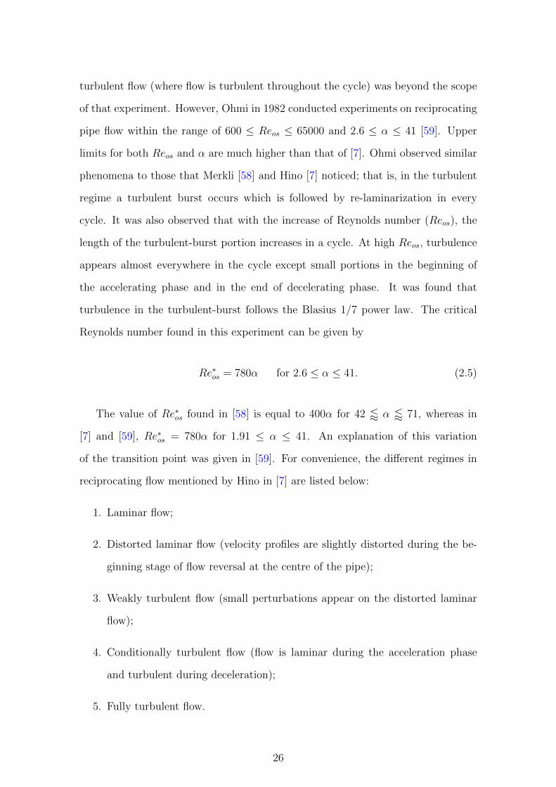
Figure 2.7. Traces of velocity variation at Reδ = 1530(Reos = 5830) and λ = 1.91[7].

24

acceleration phase and turbulent during deceleration) and fully turbulent flow (flow

is turbulent throughout the cycle). These flow types will be detailed shortly. Figure

2.7 shows the velocity profiles at different phases in a conditionally turbulent flow.

It shows that the flow drastically changes from laminar to turbulent in the beginning

of the deceleration period. However, re-laminarization occurs during the reversal of

flow direction and flow remains laminar throughout the acceleration period.

Results from the experiments were used to demarcate the flow regimes on Reos-λ

and Reδ-λ stability diagrams as shown in Figure 2.8. This shows that the transition

from laminar to weakly turbulent flow occurs at lower Reos as λ becomes higher.

However, the transition from weakly turbulent to conditionally turbulent flow takes

place at Reδ = 550, i.e.,

Re∗δ = 550 (2.3)

or,

Re∗os = 780α for 1.91 ≤ α ≤ 8.75. (2.4)

In the above-mentioned work, the highest value of Reos that was investigated

is 5830, which is in the conditionally turbulent flow regime. To study the fully

Figure 2.8. Stability diagrams: Reos vs. λ (left) and Reδ vs. λ (Right). ◦, laminaror distorted laminar flows; •, weakly turbulent flow; •+, conditionally turbulent flow[7].

25

turbulent flow (where flow is turbulent throughout the cycle) was beyond the scope

of that experiment. However, Ohmi in 1982 conducted experiments on reciprocating

pipe flow within the range of 600 ≤ Reos ≤ 65000 and 2.6 ≤ α ≤ 41 [59]. Upper

limits for both Reos and α are much higher than that of [7]. Ohmi observed similar

phenomena to those that Merkli [58] and Hino [7] noticed; that is, in the turbulent

regime a turbulent burst occurs which is followed by re-laminarization in every

cycle. It was also observed that with the increase of Reynolds number (Reos), the

length of the turbulent-burst portion increases in a cycle. At high Reos, turbulence

appears almost everywhere in the cycle except small portions in the beginning of

the accelerating phase and in the end of decelerating phase. It was found that

turbulence in the turbulent-burst follows the Blasius 1/7 power law. The critical

Reynolds number found in this experiment can be given by

Re∗os = 780α for 2.6 ≤ α ≤ 41. (2.5)

The value of Re∗os found in [58] is equal to 400α for 42 / α / 71, whereas in

[7] and [59], Re∗os = 780α for 1.91 ≤ α ≤ 41. An explanation of this variation

of the transition point was given in [59]. For convenience, the different regimes in

reciprocating flow mentioned by Hino in [7] are listed below:

1. Laminar flow;

2. Distorted laminar flow (velocity profiles are slightly distorted during the be-

ginning stage of flow reversal at the centre of the pipe);

3. Weakly turbulent flow (small perturbations appear on the distorted laminar

flow);

4. Conditionally turbulent flow (flow is laminar during the acceleration phase

and turbulent during deceleration);

5. Fully turbulent flow.

26

Ohmi in [59], considered the above-mentioned type 1 as the laminar region, types 2

and 3 as the transitional region and types 4 and 5 as the turbulent region. It was

assumed in [59] that Merkli in [58] found the transition point between laminar and

distorted laminar regions. However, Sergeev in [6], Hino in [7] and Ohmi in [59]

found the transition point between distorted laminar and weakly turbulent regions.

Another experiment on transition to turbulence in reciprocating pipe flow was

done by Eckmann in 1991 [8]. A vertical circular tube was used to investigate the

reciprocating flow. To oscillate the flow in the vertical tube, a piston arrangement

was used, as shown in Figure 2.9. Experiments were conducted for a wide range of

dimensionless amplitude A0 = 2X0/D (2.4 ≤ A0 ≤ 21.6), where X0 is the piston

stroke distance, and for a wide range of α (8.9 ≤ α ≤ 32.2). It was noted that the

flow is axisymmetric at α = 17.9, A0 = 9.6; thus at Rδ =√

2A0α = 243. The effects

of the test section entrance on the flow were found to be negligible.

Figure 2.9. Schematic diagram of the experimental set-up used in [8].

27

The critical Reynolds number was found at

Re∗δ = 500 (2.6)

or,

Re∗os = 707α for 8.9 ≤ α ≤ 32.2, (2.7)

which is close to the Sergeev’s finding in [6]. It was found that the transition process

initially starts in the boundary layer region and slowly propagates inward with the

increase of Reynolds number. Flow remains laminar in the middle section of the

pipe for 500 < Reδ < 1310, while the flow near the wall is turbulent. Additionally,

within this range of Reδ, the boundary-layer turbulence is only apparent during the

deceleration phase. As the flow changes its direction, turbulence disappears and

flow becomes laminar everywhere in the pipe.

While Eckmann investigated the reciprocating pipe flow for an upper limit of

Reδ = 1310 [8], in the same year Akhavan performed experiments on reciprocating

pipe flow for an upper limit of Reδ = 2000 [9]. However in [9], the study was done

for much lower values of Womersley number α (7 ≤ α ≤ 15) than that of [8]. It has

Figure 2.10. Phase variation of the ensemble-averaged axial velocity compared tolaminar flow theory (Reδ = 1080, α = 15) [9].

28

been found that within these ranges of Reδ and α, flow remains in the conditionally

turbulent flow regime (mentioned above). Like Eckmann, Akahvan also observed

that the turbulence appears during the deceleration phase and remains confined

near the wall region. Figure 2.10 shows that even at Reδ far above the transition

point (550) flow in the middle of the pipe is almost laminar. However, near the wall

flow is turbulent during the deceleration phase.

Additionally, Das in 1998 conducted experiments on reciprocating pipe flow [60].

This reconfirmed the different flow regimes in reciprocating flow mentioned in [7].

Like Ohmi [59], Das has also assumed that Merkli [58] found the transition point

between the laminar and distorted laminar flow. It has also been shown in [60] that

the critical Reynolds numbers Re∗δ becomes independent of α for α > 2√

2, i.e., for

δ < R/2.

2.3.2 Entrance length

This section focuses on the entrance length in reciprocating pipe flow. Numerous

studies have been conducted to express the entrance length in unidirectional pipe

flow as a function of Reynolds number [61]. However, very few works have been

done to determine the entrance length in reciprocating flow.

In 1971, Gerrard studied the flow developing length in reciprocating flow and

compared that with the developing length in steady flow [10]. The flow is consid-

ered fully developed when 100 × (u∞ − u)/(u∞ − u0) becomes equal to 1, where

u∞ is the established velocity on the centreline of the pipe, u is the local velocity

and u0 is the entry velocity. Usually the tube radius (R) is used as the characteris-

tic length to determine entry length. However, Gerrard introduced a dimensionless

length x/(R2u0/ν) (x is the distance on the centreline from the entry) so that the

dimensionless velocity on the centreline, (u∞−u)/(u∞−u0) in a steady flow becomes

a universal function of x/(R2u0/ν). The dimensionless velocity, (u∞−u)/(u∞−u0),

in both reciprocating flow and in steady flow has been plotted as a function of

x/(R2u0/ν) in Figure 2.11. This shows that the entrance length in reciprocating

29

Figure 2.11. Dimensionless velocity as a function of dimension length from theentry [10].

flow is smaller than the entrance length in steady flow. According to Gerrard, the

entrance length in reciprocating flow is smaller because the vorticity generated at

the entrance diffuses only across the boundary-layer thickness δ =√

2ν/ω. How-

ever, it has been shown that if the characteristic length is changed from R to δ for

reciprocating flow, the flow developing length in reciprocating flow coincides with

the flow developing length in steady flow.

In [62], an Ultrasonic Velocity Profile (UVP) method has been used to study the

entrance length in reciprocating pipe flow. A fast Fourier transform of the oscillating

frequency near the entrance region was applied to measure the entrance length. It

has been found that the entrance length measured using the UVP method is close

to the entrance length obtained by Gerrard in [10].

2.3.3 Energy loss due to shear stress and entrance effects

Oscillation of flow in a pipe faces resistance from different sources which require the

the application of extra force to maintain a constant amplitude. These sources are

the viscous shear stress, turbulent shear stress and the vortices at the entrance. In

this section, works related to the energy loss in reciprocating pipe flow due to shear

30

stress and entrance effects are highlighted.

Ury in 1962 derived an analytical model to calculate the friction factor in the

reciprocating flow in U-tubes [63]. It has been shown that in the conditionally

turbulent region the friction factor Cf can be expressed in terms of Reos as

Cf = 0.0791Re−0.25os . (2.8)

The damping ratio due to viscosity in the mass-spring-damping equation has been

evaluated both theoretically and experimentally. It has been found that the damping

ratio decreases with the increase of Womersley number (α).

In [11], Knott and Mackley conducted an experimental study on the vortex for-

mation at the entrance of a vertical tube, while the flow in the tube is reciprocating.

Vortices generated at the entrance have been visualised and their dynamics have

been explained. It has been shown that at a sharp entrance, separation occurs

during both in-flow and out-flow which results in the formation of vortex rings. A

schematic diagram of the vortex formation at the tube-entrance due to free oscilla-

tion is represented in Figure 2.12 from [11]. It shows that at the end of first down-

stroke a free vortex ring is formed just outside the tube-entrance (Figure 2.12(d)).

As the flow begins to move upward, another vortex ring is formed just inside the

tube-entrance (Figure 2.12(e)). Initially this vortex ring is located close to the inner

walls of the tube. However, at the beginning of the second down-stroke, this inner

vortex ring is concentrated in the centre and fluid passes between the ring and the

inner walls (Figure 2.12(f)). As the flow continues its journey downward, the first

vortex ring that was formed during the first down-stroke convects downward from

the entrance and a new vortex ring is formed outside the entrance (Figure 2.12(g)).

In a similar fashion, during the second up-stroke the vortex ring that was formed in

the first up-stroke moves upward and a new vortex ring is formed inside the entrance

(Figure 2.12(h)). It has been observed that as the oscillation continues, more new

rings are formed and the old rings move further away from the entrance.

The cycle-averaged energy dissipation due to the vortices at the entrance has

31

Figure 2.12. Schematic diagram of eddy formation at the tube entrance due tofree oscillation of water column [11].

32

been found to be

Ee = 1.24ρAU30 (2.9)

in [11], where ρ is the fluid density, A is the cross-sectional area and U0 is the

amplitude of the cross-sectional area averaged velocity. The damping ratio due to

the vortices in the mass-spring-damping equation has been calculated as

ζe =1

4π

energy extracted per cycle of forced oscillation

net energy participating in the cycle, (2.10)

and it was found that ζe = 0.2U0/ωlc, where lc is the length of the water column

inside the tube.

Another experimental study on measuring the energy dissipation due to vortices

at the entrance of a vertical pipe has been presented in [12]. Total power loss due

to all sources of damping has been expressed as

Eew =1

2CU2

0 + 0.212KeρU30 , (2.11)

where C is a linear damping coefficient and Ke is the proportion of kinetic energy

being dissipated at the entrance. The first term in equation (2.11) represents the loss

due to linear damping, whereas the second term represents the loss due to non-linear

damping. It has been presumed that the presence of linear damping is because of

viscous shear stress at the wall and the radiation of waves outside the pipe; and the

non-linear damping results from the vortices generated at the pipe-entrance. Several

factors have been pointed out that govern the amount of energy loss; these are the

frequency of oscillation, the radius of the pipe lips and of the pipe itself, and the

Reynolds number.

In [64], the total power loss (Eew) in a oscillatory flow has been estimated by

measuring the fluid resistance (Ros), which has been derived as,

Ros =

∫ T0

(p1 − p2)Qosdt∫ T0Q2osdt

, (2.12)

33

where p1 − p2 is the pressure difference, Qos is the oscillation flow rate and T is the

oscillation period. The rate of energy loss has been connected to the fluid resistance

as

Eew = Ros1

T

∫ T

0

Q2osdt. (2.13)

It has been found that the fluid resistance in oscillatory flow (Ros) is connected

to the fluid resistance in laminar Poiseuille flow (Rlam) as

Ros

Rlam

=1

1 + 0.25α1.5+ 0.166α1.49 ± 6% for 0 ≤ α ≤ 1000, (2.14)

where Rlam = 128µlc/πD4 with lc is the tube length and D is the tube diameter;

and α = D2

√ω/ν is the Womersley number.

Some works are available in the literature that have not directly measured the

energy loss in the time-dependent flows, but here measured the friction factor. This

friction factor in reciprocating flows can be interpreted as a viscous loss at the

wall. Therefore, works that measured the friction factor in oscillatory flow will be

mentioned below.

In [65], the wall shear stress has been estimated by measuring the pressure gra-

dient (∂p/∂x) and cross-sectional mean velocity (uav), and then substituting them

in

u2∗ =

τwρ

=1

2R

(−1

ρ

∂p

∂x− ∂uav

∂t

), (2.15)

where

uav(ωt) =2

R2

∫ R

0

u(r, ωt)rdr = U0sin(ωt),

u∗ is the friction velocity, τw is the wall shear stress, p is the mean pressure. It

has been found that in the laminar regime for any specific Womersley number (α),

the cycle-averaged friction factor (Cf ) decreases linearly with the increase of oscil-

latory Reynolds number (Reos = U0D/ν); and for a specific Reos, Cf increases with

α. However, in the conditionally turbulent regime (as mentioned in section 2.3.1),

during the turbulent burst it has been found that Cf can be estimated from the

34

Figure 2.13. Phase variation of the wall-frictn velocity calculated by various meth-ods: —, expression (2); ooo, −ν∂u/∂r|r=R; ....., u′v′ at y/R = 0.1;− • −, laminartheory or quasi steady turbulence correlation [9].

correlation, Cf = 0.1392Re−0.25os . It has also been shown that this correlation can be

used throughout the cycle if Reos ' 2800α for 4 / α / 24.

In [9], the wall shear stress in reciprocating pipe flow has been measured and then

compared with well-established theories. For Reδ = U0δ/ν = 1080, recalling that

(δ =√

2ν/ω) and α = 15, a wall shear stress given by −ν∂u/∂r|r=R, the Reynolds

shear stress u′v′ at y/R = 0.1, and the shear stress from the laminar theory are

all presented in Figure 2.13. Values of τw/ρ are positive for the first half cycle and

negative for the second half. This is simply due to the reversal of flow direction

in the second half. It shows that the wall friction velocity during the acceleration

period agrees with the solution of Uchida, presented in [32]. During the deceleration

period the turbulent burst mentioned in section 2.3.1 takes place, and in this region

the experimental wall friction velocity agrees with the Blasius correlation,

τwρ

= 0.03325u2av

(Ruavν

)−0.25

. (2.16)

In [29] the friction coefficient in laminar oscillatory flow has been measured

experimentally and compared with the theoretical results presented in [32]. It has

35

been found that though the velocity profiles in fully developed flow are only functions

of the Womersley number α, and the friction coefficients are function of both α and

the dimensionless amplitude of fluid A0 = Xm/D, where Xm is the maximum fluid

displacement. Experimental results agreed with the theory and showed that the

friction coefficient decreases exponentially with the increase of α.

36

Chapter 3

Analytic representations of

dissipation in OWCs

The material of this chapter is presently under review as a journal paper.

As already noted, most OWCs are designed to resonate at incoming wave fre-

quencies, so that efficiency of the device should be the maximum. However, the

damping factors, which control the efficiency of the OWCs, are not clearly identified

and modelled. Therefore, an extensive study of the internal fluid dynamics of an

OWC is required to identify those damping factors, and furthermore, to estimate

the amount of energy loss due to their presence in OWCs.

As introduced in Chapter 1, the basic working principle of a general OWC is

identical to a forced mass-spring-damping system, where the water column repre-

sents the mass, and the body force of it (due to gravity) plays the role of the spring

restoring force. And the damping term is composed of the energy losses at different

parts of the OWC. As described in Chapter 2, as the incident wave hits the device,

it creates vortices at the free-end, which carry away some energy with it. Due to

the turbulence and wall shear stresses inside the device, energy dissipates. Pressure

fluctuation in the air chamber causes a secondary wave to radiate away energy from

the OWC. A major part of the damping comes from the Power-Take-Off (PTO)

system, which is, in general, the turbine-generator arrangement. Additionally if the

37

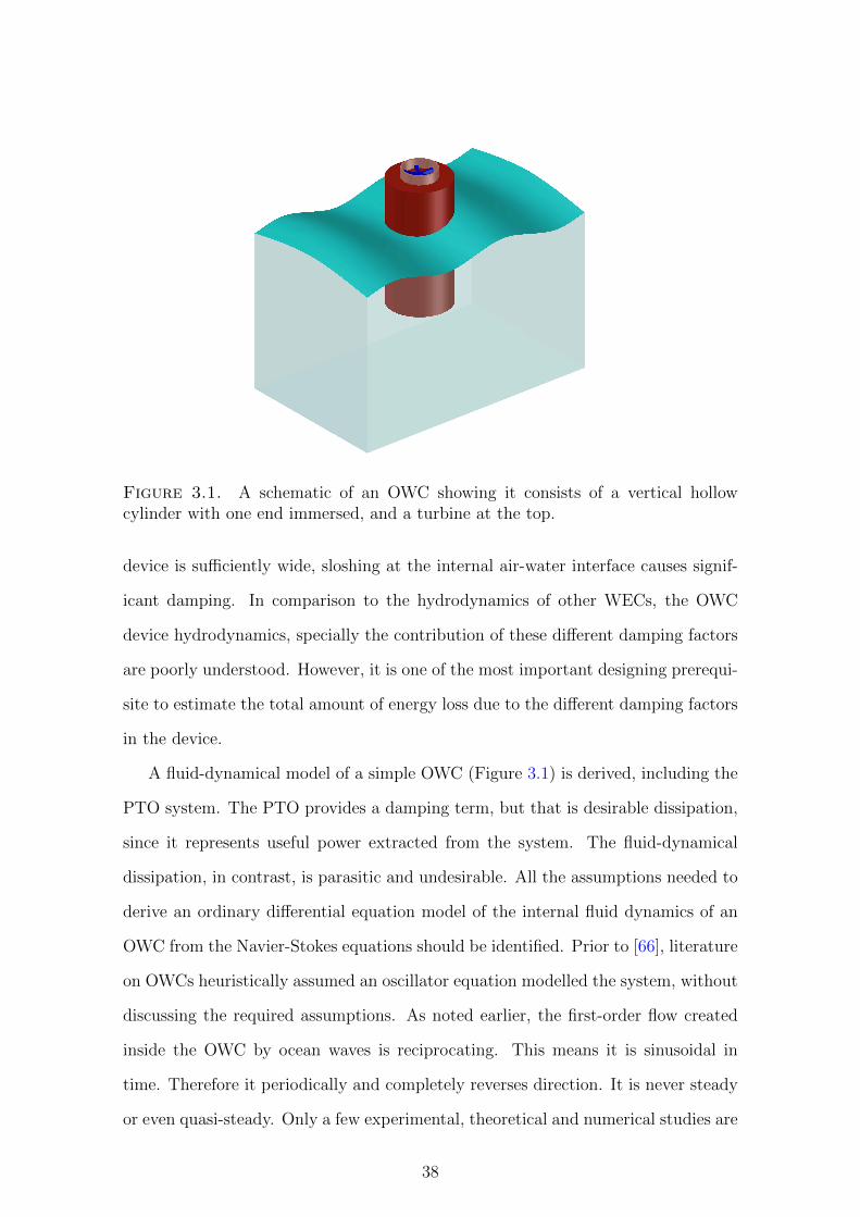
Figure 3.1. A schematic of an OWC showing it consists of a vertical hollowcylinder with one end immersed, and a turbine at the top.

device is sufficiently wide, sloshing at the internal air-water interface causes signif-

icant damping. In comparison to the hydrodynamics of other WECs, the OWC

device hydrodynamics, specially the contribution of these different damping factors

are poorly understood. However, it is one of the most important designing prerequi-

site to estimate the total amount of energy loss due to the different damping factors

in the device.

A fluid-dynamical model of a simple OWC (Figure 3.1) is derived, including the

PTO system. The PTO provides a damping term, but that is desirable dissipation,

since it represents useful power extracted from the system. The fluid-dynamical

dissipation, in contrast, is parasitic and undesirable. All the assumptions needed to

derive an ordinary differential equation model of the internal fluid dynamics of an

OWC from the Navier-Stokes equations should be identified. Prior to [66], literature

on OWCs heuristically assumed an oscillator equation modelled the system, without

discussing the required assumptions. As noted earlier, the first-order flow created

inside the OWC by ocean waves is reciprocating. This means it is sinusoidal in

time. Therefore it periodically and completely reverses direction. It is never steady

or even quasi-steady. Only a few experimental, theoretical and numerical studies are

38

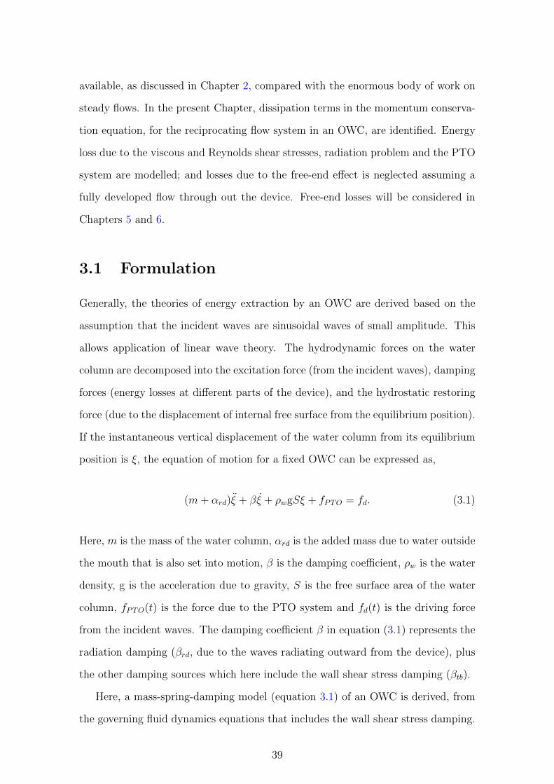
available, as discussed in Chapter 2, compared with the enormous body of work on

steady flows. In the present Chapter, dissipation terms in the momentum conserva-

tion equation, for the reciprocating flow system in an OWC, are identified. Energy

loss due to the viscous and Reynolds shear stresses, radiation problem and the PTO

system are modelled; and losses due to the free-end effect is neglected assuming a

fully developed flow through out the device. Free-end losses will be considered in

Chapters 5 and 6.

3.1 Formulation

Generally, the theories of energy extraction by an OWC are derived based on the

assumption that the incident waves are sinusoidal waves of small amplitude. This

allows application of linear wave theory. The hydrodynamic forces on the water

column are decomposed into the excitation force (from the incident waves), damping

forces (energy losses at different parts of the device), and the hydrostatic restoring

force (due to the displacement of internal free surface from the equilibrium position).

If the instantaneous vertical displacement of the water column from its equilibrium

position is ξ, the equation of motion for a fixed OWC can be expressed as,

(m+ αrd)ξ + βξ + ρwgSξ + fPTO = fd. (3.1)

Here, m is the mass of the water column, αrd is the added mass due to water outside

the mouth that is also set into motion, β is the damping coefficient, ρw is the water

density, g is the acceleration due to gravity, S is the free surface area of the water

column, fPTO(t) is the force due to the PTO system and fd(t) is the driving force

from the incident waves. The damping coefficient β in equation (3.1) represents the

radiation damping (βrd, due to the waves radiating outward from the device), plus

the other damping sources which here include the wall shear stress damping (βtb).

Here, a mass-spring-damping model (equation 3.1) of an OWC is derived, from

the governing fluid dynamics equations that includes the wall shear stress damping.

39

For convenience, the variables in the mass and momentum conservation equations

are scaled to get the dimensionless equations.

The lengths in the cylindrical co-ordinate system, x∗i = (x∗, r∗, φ) are scaled as

follows,

x∗i = Dxi,

where “*” represents dimensional quantities and D is the diameter of the device.

Time, velocity and pressure are scaled with the bar representing the mean flow,

while primes represent fluctuating variables as follows,

t∗ = ω−1t,

u∗i = ωD(Ui + u′i

), (3.2)

p∗ = ρwgD(p+ p′),

where ω is the incident wave frequency and the velocity components are defined

as u∗i = (u∗, v∗, w∗). After scaling and ensemble averaging, the mass and momen-

tum conservation equations for the incompressible flow in the water column can

respectively be written as,

∇jUj = 0, (3.3)

∂Ui∂t

+ Uj∇jUi = − g

ω2D∇ip+

1

Reω

(∇2j Ui)−∇ju′iu

′j +

giω2D

, (3.4)

where the kinetic Reynolds number, Reω = ρwωD2/µ. The required steps to derive

equations (3.3) and (3.4) from the basic Navier-Stokes equations are presented in

Appendix A.1.1.

40

3.1.1 Simplifying the x-momentum equation of the water

column

It is assumed that the water flow in the device is an axisymmetric flow. Thus the

change of any variable in the φ-direction is considered to be zero, i.e. ∂()/∂φ = 0.

Including this axisymmetric flow assumption to equation (3.3) reduces the continuity

equation to

∂U

∂x+

1

r

∂(rV )

∂r= 0, (3.5)

where V is the mean radial flow. Assuming that the device is long enough to neglect

the flow development region at the entrance and therefore the internal flow is fully-

developed throughout the OWC, ∂()/∂x = 0. Applying this fully-developed flow

assumption to (3.5) gives V = const. in the radial direction. Since V = 0 at the

wall (the no-penetration boundary condition), it is null everywhere in the device at

any given time.

After all these simplifications, the x-component of equation (3.4) becomes

∂U

∂t= − g

ω2D

∂p

∂x+

1

Reω

[1

r

∂

∂r

(r∂U

∂r

)]− 1

r

∂

∂r

(ru′v′

)+

gxω2D

. (3.6)

The 3rd and 4th terms in equation (3.6) represent the viscous and turbulent (or

Reynolds) shear stress respectively. These two shear stress terms are combined and

defined as the overall shear stress

τ =1

Reω

∂U

∂r− u′v′.

In the mass-spring-damping model, the damping due to shear stress comes from this

τ . Introducing τ into equation (3.6) gives,

∂U

∂t= − g

ω2D

∂p

∂x+

1

r

∂(rτ)

∂r+

gxω2D

. (3.7)

Since the velocity in the radial direction, V = 0, it can be shown from the r-

41

component of equation (3.4) that the pressure is constant in the radial direction, i.e,

p(r) = const. Thus, in this OWC system, pressure is a function of x and t only.

To address the aim of this work, an ordinary differential equation that consists

of only the time-dependent variables is required. However in equation (3.7), the

velocity U and the shear stress τ , are functions of both t and r. And as mentioned

above, the pressure p is a function of t and x. To make U and τ independent of the

radial coordinate, we first take the area-average of equation (3.7). This is done by

multiplying it with 2πr and then integrating with respect to r between limits 0 and

R/D and then dividing by π(R/D)2. This process gives,

dUbdt

= − g

ω2D

∂p

∂x− 4τw +

gxω2D

, (3.8)

where τw is the dimensionless wall shear stress. The bulk mean velocity Ub(t) is,

Figure 3.2. Schematic of the OWC duct device

Ub =1

π(R/D)2

∫ R/D

0

(U)2πrdr.

Henceforth, Ub(t) is expressed as ξ(t), where ξ(t) is the displacement of the free

surface inside the OWC. Furthermore, integration of equation (3.8) with respect to

42

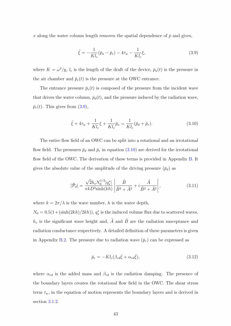
x along the water column length removes the spatial dependence of p and gives,

ξ = − 1

Klc(pa − pe)− 4τw −

1

Klcξ, (3.9)

where K = ω2/g, lc is the length of the draft of the device, pa(t) is the pressure in

the air chamber and pe(t) is the pressure at the OWC entrance.

The entrance pressure pe(t) is composed of the pressure from the incident wave

that drives the water column, pd(t), and the pressure induced by the radiation wave,

pr(t). This gives from (3.9),

ξ + 4τw +1

Klcξ +

1

Klcpa =

1

Klc(pd + pr). (3.10)

The entire flow field of an OWC can be split into a rotational and an irrotational

flow field. The pressures pd and pr in equation (3.10) are derived for the irrotational

flow field of the OWC. The derivation of these terms is provided in Appendix B. It

gives the absolute value of the amplitude of the driving pressure (pd) as

|Pd| =√

2hsN1/20 |q∗s |

πkD3sinh(kh)

∣∣∣∣∣ B

B2 + A2+ i

A

B2 + A2

∣∣∣∣∣ , (3.11)

where k = 2π/λ is the wave number, h is the water depth,

N0 = 0.5(1+(sinh(2kh)/2kh)), q∗s is the induced volume flux due to scattered waves,

hs is the significant wave height and, A and B are the radiation susceptance and

radiation conductance respectively. A detailed definition of these parameters is given

in Appendix B.2. The pressure due to radiation wave (pr) can be expressed as

pr = −Klc(βrdξ + αrdξ), (3.12)

where αrd is the added mass and βrd is the radiation damping. The presence of

the boundary layers creates the rotational flow field in the OWC. The shear stress

term τw, in the equation of motion represents the boundary layers and is derived in

section 3.1.2.

43

Substituting the radiation induced pressure pr(t) by βrd(ω) and αrd(ω) into equa-

tion (3.10) gives the form of the governing equation of motion including radiation

and shear stress damping as

(1 + αrd)ξ + βrdξ + 4τw +1

Klcξ +

1

Klcpa =

1

Klcpd. (3.13)

3.1.2 Modelling the wall shear stress, τw(t) in the recipro-

cating flow system of the OWC

The flow created inside the OWC by ocean waves is reciprocating. A reciprocat-

ing flow cycle consists of an acceleration and a deceleration phase in the positive

direction, and the same sequence in the reverse direction, giving two acceleration

and two deceleration periods. Like steady flow, the reciprocating flow might be

laminar, weakly turbulent or fully turbulent throughout the cycle, depending on the

Reynolds number, as was noted in the literature reviewed in Chapter 2. However,

Hino in [7] introduced a new flow regime in reciprocating flow, called the condi-

tional turbulence regime. In this regime, a portion of the flow cycle is laminar and

the other portion is turbulent. As Reδ = Ubδ/ν goes above 550, where the Stokes

0 π/2 π 3π/2 2π

u*

ω t*Figure 3.3. Schematic illustration of velocity at different phases in a conditionallyturbulent flow system of OWC

44

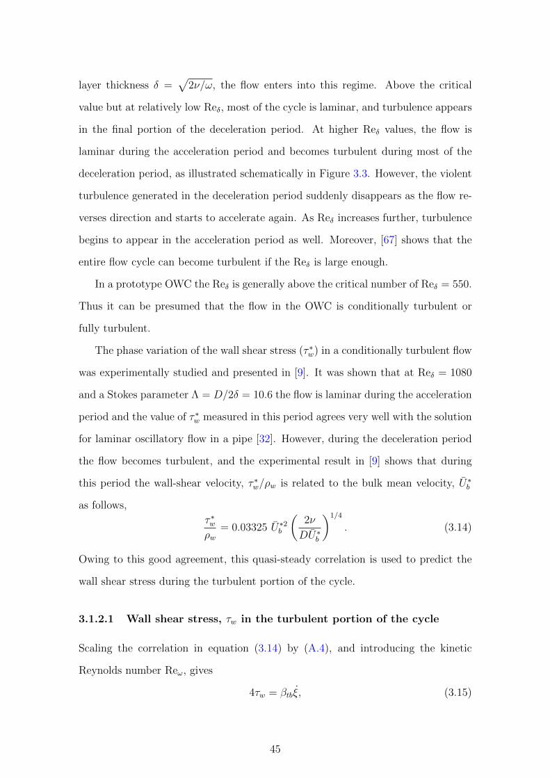
layer thickness δ =√

2ν/ω, the flow enters into this regime. Above the critical

value but at relatively low Reδ, most of the cycle is laminar, and turbulence appears

in the final portion of the deceleration period. At higher Reδ values, the flow is

laminar during the acceleration period and becomes turbulent during most of the

deceleration period, as illustrated schematically in Figure 3.3. However, the violent

turbulence generated in the deceleration period suddenly disappears as the flow re-

verses direction and starts to accelerate again. As Reδ increases further, turbulence

begins to appear in the acceleration period as well. Moreover, [67] shows that the

entire flow cycle can become turbulent if the Reδ is large enough.

In a prototype OWC the Reδ is generally above the critical number of Reδ = 550.

Thus it can be presumed that the flow in the OWC is conditionally turbulent or

fully turbulent.

The phase variation of the wall shear stress (τ ∗w) in a conditionally turbulent flow

was experimentally studied and presented in [9]. It was shown that at Reδ = 1080

and a Stokes parameter Λ = D/2δ = 10.6 the flow is laminar during the acceleration

period and the value of τ ∗w measured in this period agrees very well with the solution

for laminar oscillatory flow in a pipe [32]. However, during the deceleration period

the flow becomes turbulent, and the experimental result in [9] shows that during

this period the wall-shear velocity, τ ∗w/ρw is related to the bulk mean velocity, U∗b

as follows,

τ ∗wρw

= 0.03325 U∗2b

(2ν

DU∗b

)1/4

. (3.14)

Owing to this good agreement, this quasi-steady correlation is used to predict the

wall shear stress during the turbulent portion of the cycle.

3.1.2.1 Wall shear stress, τw in the turbulent portion of the cycle

Scaling the correlation in equation (3.14) by (A.4), and introducing the kinetic

Reynolds number Reω, gives

4τw = βtbξ, (3.15)

45

where βtb = 0.15816 Re−1/4ω |ξ|3/4. Substituting equation (3.15) into (3.13) gives the

governing equation of motion including turbulent wall shear stress and radiation

damping,

(1 + αrd) ξ + (βrd + βtb) ξ +1

Klcξ +

1

Klcpa =

1

Klcpd. (3.16)

3.1.2.2 Wall shear stress, τw in the laminar portion of the cycle

The wall shear stress, τw in the laminar period of a cycle in the fully developed

reciprocating flow is derived from Uchida’s analytic solution in [29], which can be

given as,

τ ∗wρw

= 8ωDFωU∗f sin(θ + θ1), (3.17)

where U∗f = ξ∗/sinθ; θ is the phase angle; θ1 = tan−1[(α−2C1)/(2C2)]−tan−1(C2/C1)

is the phase difference and the factor

Fω =

√C2

1 + C22

16√

(α− 2C21)2 + 4C2

2

. (3.18)

Here

C1 =ber(α)

d

dαbei(α)− bei(α)

d

dαber(α)

ber2(α) + bei2(α), C2 =

ber(α)d

dαber(α) + bei(α)

d

dαbei(α)

ber2(α) + bei2(α),

‘ber’ and ‘bei’ are the Kelvin functions and α =√

Reω/2. Introducing the scaling

factors of (3.3) into equation (3.17) gives

4τw = αlmξ + βlmξ, (3.19)

where αlm = 32Fωsin θ1 and βlm = 32Fωcos θ1. Substituting equation (3.19) into

equation (3.13) gives the governing equation of motion including laminar wall shear

stress as well as radiation damping,

(1 + αrd + αlm) ξ + (βrd + βlm) ξ +1

Klcξ +

1

Klcpa =

1

Klcpd. (3.20)

46

3.1.3 Modelling the Power-Take-Off (PTO)

To compute the pressure in the air chamber pa(t), a relationship between the PTO

performance and the hydrodynamic parameters is required. Owing to the low fre-

quency of the sea waves and high sound speed in the air, pa(t) is approximately

uniform throughout the chamber. Thus the air flow rate through the turbine is

m∗ = −d(ρaV∗)

dt∗, (3.21)

where ρa is the air density and V ∗(t) is the time-dependent air volume inside the

chamber. Following [68], the air in the chamber is considered as an ideal gas which

compresses and expands insentropically. Thus equation (3.21) can be rewritten as

m∗ = ρaQ∗ − S(lac − ξ∗)

1

c∗2dp∗adt∗

(3.22)

where the air volume rate, Q∗ = Sξ∗, lac is the length of the air chamber and c∗ is

the speed of sound in air.

It is assumed that a Wells turbine is installed in the PTO system. In [31], it is

shown that the dimensional mass flow rate through the Wells turbine, m∗/(ρaN∗t d

30)

maintains a linear relationship with the dimensionless pressure difference across it,

p∗a/(ρaN∗2t d

20); which gives

m∗ =Ktd0

N∗tp∗a, (3.23)

where N∗t is the turbine rotational speed, d0 is the turbine rotor diameter and Kt is

an empirical turbine coefficient which is fixed for a given turbine geometry.

It is also assumed that ξ∗ is very small in comparison to lac; thus combining (3.22)

and (3.23) and introducing scaling factors from (3.3) gives the ordinary differential

equation for the air pressure as

dpadt

+ 4c2Ktd0

πlacNt

pa = KD2 ρac2

ρwlacξ, (3.24)

where Nt = N∗t /ω. This can be solved in conjunction with the equation of motion

47

(3.13) for the flow in the OWC.

3.2 Results

The dimensionless instantaneous power output is calculated as

P =p∗a

ρwgD× Q∗

ωD3=π

4paξ, (3.25)

and the dimensionless average power as

Pavg =1

T

∫ T

0

P (t)dt, (3.26)

where the wave period, T = 2π/ω.

The Pavg is computed for different types of damping by solving for pa and ξ from

the corresponding equations derived above. Here three models are derived:

1. “RD” (radiation) model: Equation (3.13) is solved along with equation (3.24),

neglecting the wall shear stress τw. This gives the average power output,

Pavg when the PTO and radiation damping are present but wall shear stress

damping is not present.

2. “RD+CT” (radiation plus conditional turbulence) model: In this model Pavg

is calculated for a conditionally turbulent flow (as discussed in section 3.1.2)

where the flow inside the OWC is laminar during the acceleration period and

turbulent during the entire deceleration period as shown in Figure 3.3. There-

fore, this model includes PTO, radiation and laminar wall shear stress damping

(βlm) during the acceleration period and turbulent wall shear stress damping

(βtb) during the deceleration period.

3. “RD+TB” (radiation plus full turbulence) model: Equations (3.16) and (3.24)

are solved to calculate Pavg. This model includes the PTO, radiation and

turbulent wall shear stress damping.

48

Analytically these equations are insoluble. The explicit fourth order Runge-Kutta

algorithm is used to solve them numerically.

In this section the variation of different parameters have been presented as a

function of dimensionless wave parameter Kh (= ω2h/g), device draft length lc/h

and device diameter D/h. Note, all the independent variables have been normalised

by the water depth h, although h does not appear explicitly in the equation of

motion (equation 3.13). This is because the driving pressure (pd) in the equation of

motion is a function of h (equation 3.11) and hence all the length scales (lc, D etc.)

are commonly related to h.

The above-mentioned models are solved for air chamber length to water depth

ratio lac/h = 0.5, the significant wave height to water depth ratio hs/h = 0.2 and

turbine parameter Ktd0/lacN∗t = 0.00076 s. These values have been selected as being

representative of a fixed-type near-shore OWC.

The draft to water depth ratio lc/h = 0.5 and diameter to water depth ratio

D/h = 0.15 are used for Figures 3.4-3.5.

The variation of average power output with the dimensionless parameter Kh

for the above-mentioned damping models is presented in Figure 3.4. It shows that

in the presence of the applied damping from the PTO system and the radiation

damping, the maximum dimensionless power output at resonance is 0.167 at Kh =

1.83. It also shows that the wall shear stress in RD+CT and RD+TB models does

not cause any noticeable reduction in the power output except at the resonance

frequency. At resonance the power calculated from these two models is less than

the power calculated from the RD model by 7.78% and 12.8% respectively. For

the RD+CT model the resonance occurs at the same frequency as that of the RD

model (Kh = 1.83), however for the RD+TB model, the resonance frequency moves

to slightly lower frequency at Kh = 1.825.

A comparison of radiation and turbulent damping coefficients as a function of

Kh is presented in Figure 3.5. The radiation damping coefficient (βrd) decreases

with Kh; however, the turbulent damping coefficient (βtb) increases with Kh until

49

0

0.06

0.12

0.18

0 0.5 1 1.5 2 2.5 3 3.5 4

0.13

0.14

0.15

0.16

0.17

1.72 1.76 1.8 1.84 1.88 1.92

Kh

Pavg

Figure 3.4. Average dimensionless power against dimensionless parameter Kh fordifferent damping models: , RD; , RD+CT; , RD+TB. As anexample, if the water depth h = 10 m, significant wave height hs = 2 m, for theparameters of ω = 1.34 rad/s and D = 1.5 m, the dimensional power in kW wouldbe obtained by multiplying Pavg by (ρwgωD4)/1000 = 66.55.

0

0.003

0.006

0.009

0 0.5 1 1.5 2 2.5 3 3.5 4

Kh

β

Figure 3.5. Damping coefficients as a function of Kh for lc/h = 0.5 and D/h =0.15: , βrd; , βtb.

50

it reaches the resonance frequency and then falls rapidly as Kh increases further.

Though βtb is smaller than βrd at any Kh, at resonance βtb becomes almost equal to

βrd. This indicates that at resonance both the damping sources play important role

in the device performance. However, apart from the resonance, βrd is significantly

higher than βtb in a fixed-type near-shore OWC.

The presence of wall shear stress reduces the power output in the OWC. Figure

3.6 shows the impact of wall shear stress on the power extraction at resonance for dif-

ferent submergence depth and diameter of the device. At resonance, the percentage

of energy loss due to wall shear stress increases linearly as the submergence depth of

the device increases for a fixed diameter (Figure 3.6(a)). Whereas for a certain sub-

mergence depth of the OWC, the percentage of energy loss due to wall shear stress

decreases exponentially with the increase of the diameter (Figure 3.6(b)). Both the

figures ascertain that for a constant water depth if the draft to diameter ratio (lc/D)

increases, the relative loss due to wall shear stress increases significantly.

0

5

10

15

20

25

0.2 0.3 0.4 0.5 0.6 0.7 0.8

0

10

20

30

0.1 0.2 0.3 0.4 0.5 0.6

lc/h D/h

Ener

gylo

ss(%

)

Ener

gylo

ss(%

)

(a) (b)

Figure 3.6. Energy loss due to wall shear stress (a) at different lc/h for D/h = 0.15(b) at different D/h for lc/h = 0.5. ◦ , RD+CT; • , RD+TB.

For a narrow device (large lc/D), the water column inside the OWC can be

regarded as a solid-body, and hence its motion can be assumed to be the oscillation

of a liquid pendulum. The approximate natural frequency of such a device is√

g/lc

rad/s, where lc is the length of the duct that is under water. Thus, for a purely

solid-body motion the resonance should occur at Klc = 1. For a constant D, with

the decrease of lc (device becoming shorter), the oscillation of the water column

51

Kh

Pavg

Kh

Pavg

l c/h

D/h

(a) (b)

Figure 3.7. Average dimensionless power calculated for the RD+TB model as afunction of (a) Kh and lc/h for D/h = 0.15, and (b) Kh and D/h for lc/h = 0.5.The dashed line represents the position of the peak at resonance if the water columnworks as a solid-body.

deviates more from the solid-body model. Consequently the resonance takes place

at lower Klc value than the expected one. A similar phenomenon occurs when D

is increased (the device gets wider) by keeping lc constant. This effect can be seen

from Figure 3.7 which shows contours of the average power Pavg as a function of Kh

and lc/h. According to the solid-body oscillation approximation, for D/h = 0.15

and lc/h of 0.8, 0.6 and 0.4 the resonance is expected at Kh = 1.25, 1.67 and 2.5

respectively (from the dashed line in Figure 3.7(a)); however it is occurring, as

indicated by the darkest contours, at Kh = 1.175, 1.495 and 2.135, with a deviation

of 6%, 10.48% and 14.6% respectively. For lc/h = 0.5 the solid-body approximation

suggests that resonance will always occur at Kh = 2 for any value of D/h. Figure

3.7(b) presents contours of Pavg as a function of Kh and D/h for this case. The

expected resonance at Kh = 2 is marked with a dashed line. Figure 3.7(b) shows

that with the increase of D/h while lc/h is kept constant, the oscillation deviates

from the solid-body model significantly and resonance is occurring at a lower Kh

value than the expected one.

The study of the influence of device geometry on the radiation and wall shear

stress damping is one of the most important prerequisites while designing an OWC.

52

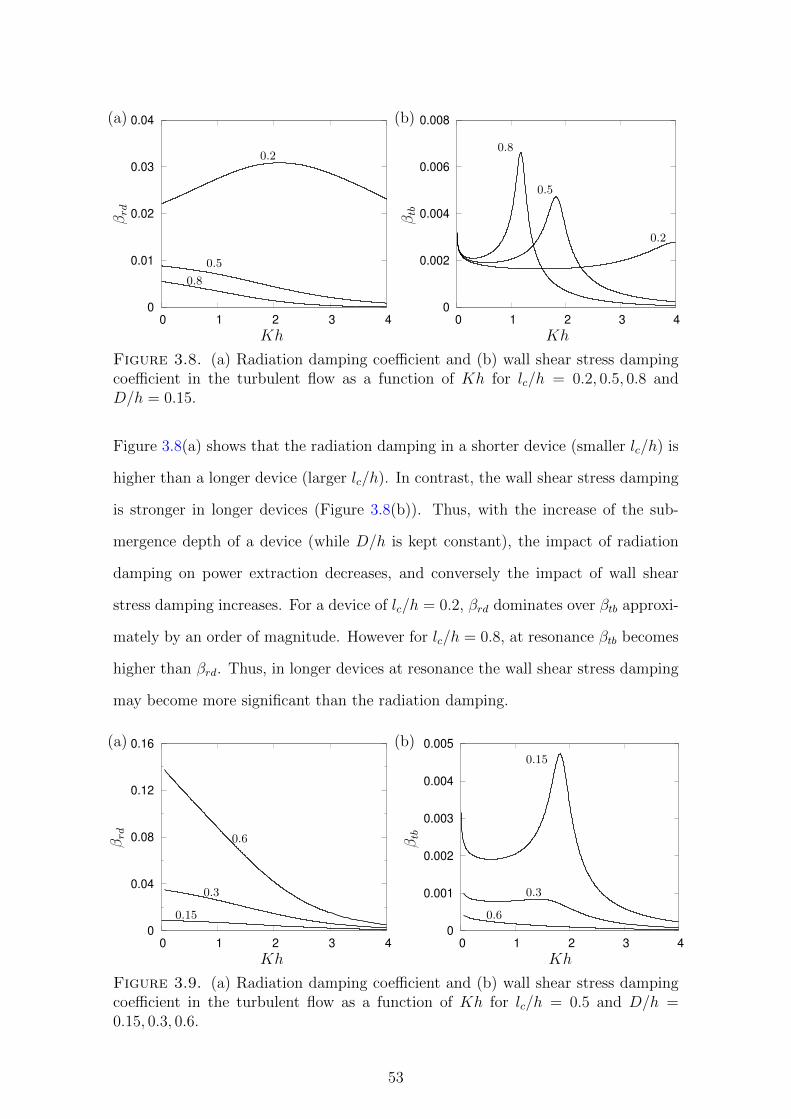
0

0.01

0.02

0.03

0.04

0 1 2 3 4

0

0.002

0.004

0.006

0.008

0 1 2 3 4

Kh Kh

βrd

βtb

0.2

0.5

0.8

0.8

0.5

0.2

(a) (b)

Figure 3.8. (a) Radiation damping coefficient and (b) wall shear stress dampingcoefficient in the turbulent flow as a function of Kh for lc/h = 0.2, 0.5, 0.8 andD/h = 0.15.

Figure 3.8(a) shows that the radiation damping in a shorter device (smaller lc/h) is

higher than a longer device (larger lc/h). In contrast, the wall shear stress damping

is stronger in longer devices (Figure 3.8(b)). Thus, with the increase of the sub-

mergence depth of a device (while D/h is kept constant), the impact of radiation

damping on power extraction decreases, and conversely the impact of wall shear

stress damping increases. For a device of lc/h = 0.2, βrd dominates over βtb approxi-

mately by an order of magnitude. However for lc/h = 0.8, at resonance βtb becomes

higher than βrd. Thus, in longer devices at resonance the wall shear stress damping

may become more significant than the radiation damping.

0

0.04

0.08

0.12

0.16

0 1 2 3 4

0

0.001

0.002

0.003

0.004

0.005

0 1 2 3 4

Kh Kh

βrd

βtb0.6

0.3

0.15

0.15

0.3

0.6

(a) (b)

Figure 3.9. (a) Radiation damping coefficient and (b) wall shear stress dampingcoefficient in the turbulent flow as a function of Kh for lc/h = 0.5 and D/h =0.15, 0.3, 0.6.

53

Additionally, Figure 3.9 shows the variation of βrd and βtb with the increase

of D/h for a constant lc/h. As the device gets wider (D/h increases) the radia-

tion damping (βrd) becomes stronger but converges slowly as Kh increases (Figure

3.9(a)). On the other hand, the wall shear stress damping (βtb) drops rapidly with

the increase of device diameter (Figure 3.9(b)). For wider devices, βrd is very much

larger than βtb. However, as the device gets narrower (D/h decreases), the difference

between these two damping coefficients decreases.

0

0.1

0.2

0.3

0.4

0.5

0 1 2 3 4

0

0.1

0.2

0.3

0.4

0.5

0 1 2 3 4

Kh Kh

|Pd|

|Pd|

0.2

0.5

0.8

0.15

0.3

0.6

(a) (b)

Figure 3.10. The amplitude of the driving pressure as a function of (a) Kh forlc/h = 0.2, 0.5, 0.8; D/h = 0.15 and (b) Kh for D/h = 0.15, 0.3, 0.6; lc/h = 0.5.

The amount of pressure that an OWC gets from the incident wave varies with the

wave frequency and also with the device dimension. Figure 3.10 shows the variation

of the amplitude of the driving pressure, |Pd| with Kh for different lc/h and D/h.

Figure 3.10(a) shows that the driving pressure from the incident wave is higher in a

shorter device (smaller lc/h) at any wave frequency. Whereas Figure 3.10(b) shows

that as the diameter of the OWC increases the incident wave pressure amplitude

at the device entrance decreases. For any dimension of the device, |Pd| decreases

exponentially with Kh, except for a rapid increase at the beginning.

Finally, the dimensionless power Pavg as a function of Kh and the significant

wave height to water depth ratio hs/h is presented in Figure 3.11. As the wave

height increases the power output from the device increases, as expected. However,

apart from the resonance this increase in power extraction is not very significant.

54

Kh

hs/h

Pavg

Figure 3.11. Average dimensionless power extracted from an OWC of lc/h =0.5 and D/h = 0.15, as a function of Kh and hs/h for the RD+TB model. Forexample, if the water depth h = 10 m and the significant wave height hs = 3 m,at resonance (ω = 1.34 rad/s) a device of lc = 5 m and D = 1.5 m can extractPavg × ρwgωD4/1000 ≈ 0.3× 66.55 ≈ 20 kW power.

Additionally, as the significant height goes higher the range of Kh over which the

resonance occurs gets wider.

In summary, though the radiation damping is the most dominant damping in

the fixed-type near-shore OWCs, the wall shear stress damping becomes significant

when the device resonates. The narrower the device (larger lc/D for a given h) the

more the oscillation of the water column inside the device gets close to the solid body

oscillation. As the device gets narrower (oscillation gets closer to solid-body) the

radiation damping decreases and consequently the average power output increases.

On the other hand, the wall shear stress damping becomes stronger as the device

gets narrower. As shown in Figure 3.6, the wall shear stress can reduce the power

extraction at resonance by more than 20% for some lc/D values.

55

3.3 Summary

Damping due to the PTO system, radiated waves, internal wall shear stress and

the flow development region at the entrance are the major damping factors in a

general OWC. Understanding these different damping factors and estimating their

contribution to the energy loss is one of the most important design prerequisites.

A mass-spring-damping model of a simple OWC is derived from the Navier-

Stokes equations that includes the damping due to the wall shear stress. The radia-

tion properties are calculated from [1] and adapted into the current model through a

conversion to the present rigid-body model. The wall shear stress damping is mod-

elled specifically for the reciprocating flow inside the OWC. An ordinary differential

equation of the air pressure inside the air chamber is derived to include the PTO

system. Since analytic modelling of the energy loss due to the developing region at

the entrance is only likely to be feasible following numerical modelling which will be

undertaken for the following Chapters, the flow is assumed fully-developed in the

present Chapter.

It is found that while the radiation damping is the most dominant damping in the

fixed-type near-shore devices, the wall shear stress damping also becomes significant

at the resonance for narrower devices. Thus the wall shear stress damping needs to

be considered while designing an OWC that resonates at the incident wave frequency.

56

Chapter 4

Entrance length in laminar

reciprocating pipe flow

As mentioned in the previous Chapter, the flow in the OWC is assumed fully devel-

oped through out the device while conducting the analytical study. In reality, there

is developing length at the free-end of the OWC. As mentioned in Chapter 1, unlike

the unidirectional flow, there is no well established correlation between the Reynolds

number and the developing length in the reciprocating flow. Thus an approach is

taken to measure the developing length at the free-end in reciprocating pipe flow.

As the flow enters into a conduit, the fluid particles close to the walls slow down

due to the no-slip boundary condition. A resistance from the slower particles close

to the walls propagates inward owing to the presence of viscosity. Consequently,

a boundary layer is generated separating the vortex dominated flow near the walls

and the free stream near the centre. As the distance from the entrance increases,

the thickness of this boundary layer becomes constant, resulting in a constant ve-

locity profile along the axis. The distance that is required for a velocity profile at

the entrance to become fully developed, (i.e., so that velocity profile does not vary

along the axis) is generally defined as the entrance length. One of the most impor-

tant prerequisites to study the fully developed flow is to know the entrance length.

Additionally, it is important to know the entrance length to estimate the energy loss

57

due to the entrance.

Numerous studies on measuring the entrance length in laminar steady flow are

available in the literature, e.g., [69–72]. Some works have been done on the esti-

mation of the entrance length in pulsatile flows with non-zero mean, e.g., [73, 74].

However, the limited application of laminar reciprocating flow in engineering prac-

tice has not made the field very attractive; thus very few works are found in the

literature that evaluated the entrance length in reciprocating flow. The analyti-

cal work on the Oscillating Water Column in Chapter 3 has raised questions like

whether the pipe entrance has significant effect on the reciprocating flow, how far

the effect continues from the entrance and so on.

As noted in Chapter 2, entrance length in a laminar reciprocating pipe flow has

been experimentally investigated by Gerrard in [10]. Experiments were conducted to

measure the entrance length at different phases of the flow cycle. The entrance length

was estimated by plotting the deviation of local velocity from the fully developed

velocity as a function of a non-dimensional distance xν/δ2u0, where x is the distance

from the entrance, δ =√

2ν/ω is the Stokes-layer thickness, u0 is the cross-sectional

mean velocity and ν is the kinematic viscosity. It has been shown that the flow

development in reciprocating flow as a function of xν/δ2u0 is almost similar to that

of the steady flow when the flow development in steady flow is plotted as a function

of xν/R2u0, where R is the pipe radius. It was also noted in Chapter 2 that a similar

result has been obtained by Yamanaka in [62] where an Ultrasonic Velocity Profile

method was used to measure the entrance length.

However, Gerrard’s experiment was limited to a Womersley number α = 12D√ω/ν

= 14.4 and the dimensionless cross-sectional mean velocity amplitude A0 = U0/ωD

= 2.6. What happens at lower α or higher A0, and how the entrance length varies

with α and A0, are not known from the literature.

In the present Chapter, a study using Direct Numerical Simulation (DNS) is

conducted to deduce the impact of α and A0 on the entrance length. The entrance

length is measured for a wide range of α (1.6 ≤ α ≤ 10) and A0 (1 ≤ A0 ≤ 9) within

58

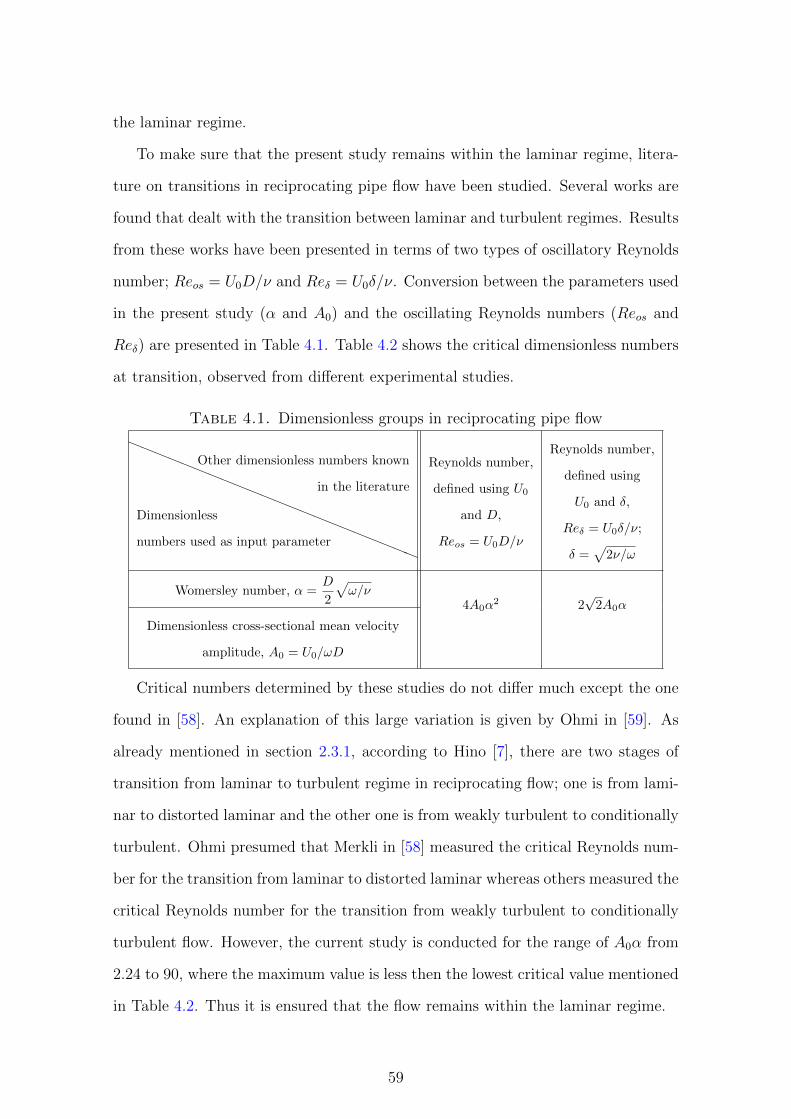
the laminar regime.

To make sure that the present study remains within the laminar regime, litera-

ture on transitions in reciprocating pipe flow have been studied. Several works are

found that dealt with the transition between laminar and turbulent regimes. Results

from these works have been presented in terms of two types of oscillatory Reynolds

number; Reos = U0D/ν and Reδ = U0δ/ν. Conversion between the parameters used

in the present study (α and A0) and the oscillating Reynolds numbers (Reos and

Reδ) are presented in Table 4.1. Table 4.2 shows the critical dimensionless numbers

at transition, observed from different experimental studies.

Table 4.1. Dimensionless groups in reciprocating pipe flow

aaaaaaaaaaaaaaaaaaaaaa

Dimensionless

numbers used as input parameter

Other dimensionless numbers known

in the literature

Reynolds number,

defined using U0

and D,

Reos = U0D/ν

Reynolds number,

defined using

U0 and δ,

Reδ = U0δ/ν;

δ =√

2ν/ω

Womersley number, α =D

2

√ω/ν

4A0α2 2

√2A0α

Dimensionless cross-sectional mean velocity

amplitude, A0 = U0/ωD

Critical numbers determined by these studies do not differ much except the one

found in [58]. An explanation of this large variation is given by Ohmi in [59]. As

already mentioned in section 2.3.1, according to Hino [7], there are two stages of

transition from laminar to turbulent regime in reciprocating flow; one is from lami-

nar to distorted laminar and the other one is from weakly turbulent to conditionally

turbulent. Ohmi presumed that Merkli in [58] measured the critical Reynolds num-

ber for the transition from laminar to distorted laminar whereas others measured the

critical Reynolds number for the transition from weakly turbulent to conditionally

turbulent flow. However, the current study is conducted for the range of A0α from

2.24 to 90, where the maximum value is less then the lowest critical value mentioned

in Table 4.2. Thus it is ensured that the flow remains within the laminar regime.

59

Table 4.2. Critical dimensionless numbers at transition

Reference Re∗os Re∗δ (A0α)∗ Range of α

[6] 700α 495 175 4 ≤ α ≤ 40

[58] 400α 283 100 42 ≤ α ≤ 71

[7] 780α 550 195 1.91 ≤ α ≤ 8.75

[59] 780α 550 195 2.6 ≤ α ≤ 41

[8] 707α 500 177 8.9 ≤ α ≤ 32.2

In the present study, the flow field is investigated in a pipe with free-ends exiting

to reservoirs as shown in Figure 4.1. All the dimensions are normalised by the pipe

diameter. The flow rate at the reservoir inlets is driven sinusoidally with time, and

equal and opposite at each end. A structured mesh of 5136 quadrilateral elements

with 64 internal points on each element is used to run the simulations. While

validating the code, it has been found that around 30% less number of elements

than the present number of elements, with 49 internal points on each element give

the same velocity profile as the theoretical velocity profile derived in [32]. The

DNS code used in the present study uses a nodal-based spectral-element method

to solve the incompressible Navier-Stokes equations. It is assumed that the flow is

axisymmetric throughout the flow domain. A more detailed description of the DNS

code is given in Appendix C.

Figure 4.1. Schematic diagram of the geometry.

60

4.1 Validation

To validate the numerical code, the axial velocity profiles in fully developed flow

obtained from the simulations are compared with analytical results. The exact

solution of the axial velocity in a fully developed reciprocating pipe flow is derived

from [32] where Uchida presented an analytical solution for the axial velocity in a

pulsating flow. Thus, the axial velocity in a fully developed reciprocating pipe flow,

as a function of α and A0 can be given as

u =4νA0α

3

D√

(α− 2C1)2 + 4C22

[B1 cosωt+ (1−B2) sinωt], (4.1)

where

B1 =bei(α)ber(2αr)− ber(α)bei(2αr)

ber2(α) + bei2(α), B2 =

ber(α)ber(2αr) + bei(α)bei(2αr)

ber2(α) + bei2(α),

C1 =ber(α)

d

dαbei(α)− bei(α)

d

dαber(α)

ber2(α) + bei2(α), C2 =

ber(α)d

dαber(α) + bei(α)

d

dαbei(α)

ber2(α) + bei2(α);

where ‘ber’ and ‘bei’ are the Kelvin functions, and r is the dimensionless radial

-0.5

0

0.5

-2 -1 0 1 2 -1.5 -1 -0.5 0 0.5 1 1.5

5π

3

2π

3

4π

3π

π

32π

5π

3

2π

3

4π

3π

π

32π

u u

r/D

(a) (b)

Figure 4.2. Comparison between theoretical results (•) and simulation results(—) of the velocity profiles in fully developed flow for (a) α′ = 4α2 = 50, A0 = 3;(b) α′ = 400, A0 = 3.

61

distance. To avoid fractional numbers while presenting the results, α is represented

by α′ = 4α2 in the rest of this Chapter.

Theoretical results from equation (4.1) and simulation results are compared for

α′ = 50 and A0 = 3 in Figure 4.2(a) and for α′ = 400 and A0 = 3 in Figure 4.2(b).

The simulation results are obtained by extracting the profile at the middle of the

pipe. It can be seen that the code can compute the velocity profile in reciprocating

pipe flow with no noticeable error.

4.2 Measuring the entrance length

The centreline velocity (uc) is generally used to measure the entrance length in pipe

flows, e.g. [10, 72]. The present study also uses the centreline velocity to measure

the entrance length. However, as an additional parameter, the transverse velocity

gradient at the wall (∂u/∂r|w) is also used to determine the entrance length. A

comparison of the centreline velocity at the pipe entrance and at the fully developed

region at different phases of the cycle is presented in Figure 4.3. It shows that

from 0 to π/2 the inflow is decelerating and from π/2 to π and from π to 3π/2

the outflow is accelerating and decelerating, respectively. From 3π/2 to 2π the

π/2

π

3π/2

2π

-1.5 -1 -0.5 0 0.5 1 1.5

uc

φ

Figure 4.3. Time history of the centreline velocity (uc) at the pipe entrance (◦)and at the fully developed region (•) for α′ = 400 and A0 = 3.

62

inflow is accelerating. It also shows that at the entrance uc is not purely sinusoidal,

however at the distance where the flow becomes fully developed, uc becomes purely

sinusoidal.

To demonstrate the evolution of both uc and ∂u/∂r|w along the pipe at different

phases of the cycle, the velocity profiles at different distance from the entrance for

α′ = 400 and A0 = 3 are presented in Figure 4.4. It shows that at φ = π/6,

which is within the decelerating period of the inflow, the velocity profile near the

entrance (x/D = 0, 1, 2) differs from the one that is in the fully developed region

(x/D = 50), i.e., both uc and ∂u/∂r|w at the entrance differ from the fully developed

values. At φ = 4π/6, which is within the accelerating period of the outflow, the

difference between the velocity profile near the entrance and in the fully developed

region becomes significant. However, this difference gradually reduces at φ = 7π/6

-0.5

0

0.5

0 0.4 0.8 0 0.4 0.8

-0.5

0

0.5

0 0.4 0.8 0 0.4 0.8

u u

u u

r/D

r/D

x/D

=0 1 2 50

x/D

=0 1 2 50

x/D

=0 1 2 50

x/D

=0 1 2 50

φ = π/6

φ = 10π/6φ = 7π/6

φ = 4π/6

Figure 4.4. Evolution of velocity profile along the pipe, at different phases of thecycle for α′ = 400 and A0 = 3.

63

and 10π/6 which belong to the decelerating period of the outflow and accelerating

period of the inflow respectively. In summary, the difference between the magnitude

of the measured variable (uc or ∂u/∂r|w) at the entrance and in the fully developed

region is more during the inflow than during the outflow.

4.2.1 Measuring techniques

Two different methods are used to measure the entrance length (le).

1. The first method is to measure the difference between uc or ∂u/∂r|w in the fully

developed region and at different locations from the entrance i.e., (uc)∞−uc or

(∂u/∂r|w)∞ − ∂u/∂r|w where the subscript ∞ represents the fully developed

value. The distance from the entrance that is required for the difference to

reduce to 0.01 will be considered as the entrance length.

2. The second method is to measure the gradient of uc and ∂u/∂r|w along the

pipe, i.e., ∂uc/∂x and ∂(∂u/∂r|w)/∂x; the distance from the entrance that

is required for the gradients to reach 0.01 will be considered as the entrance

length.

x x

(∂u/∂r)w uc

φ φ

(a) (b)

Figure 4.5. Contours of (a) ∂u/∂r|w and (b) uc for α′ = 400 and A0 = 3, as afunction of the distance from the entrance (x) and the phase variation φ; the symbols(•) show the location where (∂u/∂r|w)∞ − ∂u/∂r|w = 0.01 and (uc)∞ − uc = 0.01on the corresponding plots.

64

x x

(∂u/∂r)w uc

φ φ

(a) (b)

Figure 4.6. Contours of (a) ∂u/∂r|w and (b) uc for α′ = 400 and A0 = 3, asa function of the distance from the entrance (x) and the phase variation φ; thesymbols (•) show the location where ∂(∂u/∂r|w)/∂x = 0.01 and ∂uc/∂x = 0.01 onthe corresponding plots.

Figure 4.5 and 4.6 show the entrance lengths (le) measured by the above-mentioned

methods at different phases of the cycle for α′ = 400 and A0 = 3. The variation of le

for both the methods follows the same sinusoidal pattern with time. A comparison

of the time history of le (Figure 4.5 or 4.6) with the time history of uc (Figure 4.3)

shows that there is an approximately 90◦ phase difference between these two. During

the inflow deceleration le increases and reaches to its maximum value when the flow

changes its direction and outflow acceleration starts. Throughout the outflow (both

acceleration and deceleration periods) the entrance length decreases and reaches its

minimum when the flow changes its direction again and inflow acceleration starts.

Thus the maximum entrance length in a reciprocating pipe flow is found when the

flow changes its direction from inflow to outflow, and the minimum entrance length

is found when the flow changes its direction from outflow to inflow.

65

4.2.2 Comparing the measurement techniques

Comparison between the measured variables uc and ∂u/∂r|w, for the two measur-

ing methods, in terms of the dimensionless maximum entrance length ((le)max/D)

and cycle-average entrance length ((le)mean/D) are presented in Figure 4.7 and 4.8.

Figure 4.7 shows the results as a function of α′ for A0 = 3, while Figure 4.8 shows

the results as a function of A0 for α′ = 400.

It can be seen from both the figures that (le)max/D measured by uc and ∂u/∂r|w

varies very little from one another in both the methods. However, (le)mean/D mea-

sured by uc and ∂u/∂r|w varies up to a few diameters at higher A0 values. In all

the cases, ∂u/∂r|w measures a longer entrance length than the entrance length mea-

sured by uc. Furthermore, among the two methods, Method 2 measures a slightly

2

4

6

8

10

0 100 200 300 400

2

4

6

8

10

0 100 200 300 400

0

2

4

6

0 100 200 300 400

0

2

4

6

0 100 200 300 400

(le) m

ax/D

(le) m

ean/D

(le) m

ax/D

(le) m

ean/D

α′ α′

α′ α′

(a) (b)

(c) (d)

(∂u/∂r|w)∞ − ∂u/∂r|w = 0.01 ◦(uc)∞ − uc = 0.01 •

(∂u/∂r|w)∞ − ∂u/∂r|w = 0.01 ◦(uc)∞ − uc = 0.01 •

∂(∂u/∂r|w)/∂x = 0.01 ◦∂uc/∂x = 0.01 •

∂(∂u/∂r|w)/∂x = 0.01 ◦∂uc/∂x = 0.01 •

Figure 4.7. Maximum entrance length of the cycle, measured using (a) Method1, (b) Method 2; and the cycle-average entrance length measured using (c) Method1, (d) Method 2, as a function of α′, for A0 = 3.

66

0

5

10

15

20

25

30

0 2 4 6 8 10

0

5

10

15

20

25

30

0 2 4 6 8 10

0

4

8

12

16

20

0 2 4 6 8 10

0

4

8

12

16

20

0 2 4 6 8 10

(le) m

ax/D

(le) m

ean/D

(le) m

ax/D

(le) m

ean/D

A0 A0

A0 A0

(a) (b)

(c) (d)

(∂u/∂r|w)∞ − ∂u/∂r|w = 0.01 ◦(uc)∞ − uc = 0.01 •

(∂u/∂r|w)∞ − ∂u/∂r|w = 0.01 ◦(uc)∞ − uc = 0.01 •

∂(∂u/∂r|w)/∂x = 0.01 ◦∂uc/∂x = 0.01 •

∂(∂u/∂r|w)/∂x = 0.01 ◦∂uc/∂x = 0.01 •

Figure 4.8. Maximum entrance length of the cycle measured using (a) Method 1,(b) Method 2; and the cycle-average entrance length measured using (c) Method 1,(d) Method 2, as a function of A0, for α′ = 400.

longer entrance length than Method 1, i.e., ∂(∂u/∂r|w)/∂x measures a slightly longer

entrance length than the one measured by (∂u/∂r|w)∞ − ∂u/∂r|w.

Since there is no significant difference in entrance lengths measured by the dif-

ferent techniques, while ∂(∂u/∂r|w)/∂x estimates the longest entrance length, the

rest of this thesis uses ∂(∂u/∂r|w)/∂x to analyse the results.

4.3 Results

As noted earlier, the entrance length in laminar time-steady pipe flow has been

studied in numerous works. A general correlation between the entrance length and

the Reynolds number (Re = UD/ν) in laminar flow is given in text books, e.g.,

[61], as le/D = 0.05Re, and more precise measurements in [72] has shown that the

67

correlation is le/D = [(0.619)1.6 + (0.0567Re)1.6]1/1.6. However, the absence of such

a correlation in laminar reciprocating pipe flow provides inspiration for the analysis

of the present results in such a way that a correlation can be established.

Figure 4.9 presents the maximum entrance length to diameter ratio ((le)max/D)

as a function α′ (50 ≤ α′ ≤ 400) for A0 = 1 to 9. It shows that for any value

of A0 the lowest (le)max is at α′ = 50. It increases to the maximum at α′ = 100,

except for A0 = 9. From α′ = 100 to 200, (le)max/D decreases linearly. From

α′ = 200 to 400 for A0 = 1 to 7, (le)max/D also decreases linearly, however with a

relatively smaller slope. For α′ = 350 and 400 at A0 = 8 and 9, results deviate from

the trend at lower amplitudes. There are two possible reasons for this deviation.

Firstly, all the measurements for A0 = 1 to 7 are done in the 4th period of the flow,

however for A0 = 8 and 9 the measurements are done in the 3rd cycle, owing to

computational limitations. It may happen that the solution is not converged to a

truly periodic solution in the 3rd cycle at higher α′ for A0 = 8 and 9. Secondly,

it is possible that the flow is not in the laminar regime at α′ = 350, A0 = 8;

which is equivalent to A0α = A0

√(α′/4) = 74.83. Though this value is lower than

any critical value presented in Table 4.2, a reasonable explanation can be given to

0

5

10

15

20

25

30

100 200 300 400

9

8

7

6

5

4

3

2

A0 = 1

α′

(le) m

ax/D

Figure 4.9. Maximum entrance length to diameter ratio as a function of α′ atdifferent A0.

68

support this finding. All the works listed in Table 4.2 conducted the experiments

with a cylinder-piston arrangement, connected to the main test section with a bell

shaped entrance to measure the critical Reynolds number, i.e., with no free-ends.

However in the present study, the flow is investigated in a pipe with free-ends. Thus,

most likely the disturbance from the free-ends forces the flow to become unstable at

lower α than the previous studies have measured.

0

5

10

15

20

25

30

1 3 5 7 9

A0

(le) m

ax/D

Figure 4.10. Maximum entrance length to diameter ratio as a function of A0 forα′ = 50, × ; α′ = 100, • ; α′ = 200, + ; and α′ = 400, ◦ .

The maximum entrance length (le)max/D as a function of A0 for α′ = 50, 100, 200

and 400 is presented in Figure 4.10. It can be seen from Figure 4.9 that for α′ = 50,

with an increase of A0, (le)max/D does not increase proportionally. Thus a nonlinear

increase of (le)max/D with A0 can be seen for α′ = 50 in Figure 4.10. For α′ = 100

and 200, (le)max/D varies linearly with A0, however the slope is higher for α′ = 100

than that for 200. From α′ = 200 to 400, (le)max/D varies linearly with A0 with

very small slope difference except for α′ = 400 at A0 = 8 and 9. An explanation of

this deviation has been given while describing Figure 4.9.

A combined form of all the data shown in Figure 4.9 and 4.10 are presented in

Figure 4.11, except for α′ = 50. It is found that if the entrance length is scaled

with Stokes-layer thickness (δ =√

2ν/ω) instead of the diameter (D) and plotted

69

0

100

200

300

400

0 50 100 150 200 250 300

Reδ

(le) m

ax/δ

Figure 4.11. Maximum entrance length to Stokes-layer thickness ratio as a func-tion of Reδ for the range α′ from 100 to 400 and A0 from 1 to 9. The straight linerepresents the correlation (le)max/δ = 1.37Reδ + 5.3.

against the Reynolds number defined by δ, which is a function of both A0 and α′,

i.e., Reδ = A0

√2α′, all the data collapse to a single trend as shown in Figure 4.11.

It can be seen that the best fit for this trend is linear. Therefore a linear correlation

can be established between (le)max/δ and Reδ as, (le)max/δ = 1.37Reδ + 5.3 which

is valid for the range of α′ from 100 to 300 for 1 ≤ A0 ≤ 9 and from 300 to 400 for

1 ≤ A0 ≤ 7.

The dimensionless cycle-average entrance length ((le)mean/D) as a function of α′

and A0 is presented in Figure 4.12 and 4.13 respectively. Figure 4.12 shows that

for lower A0 values (1 to 4), (le)mean/D varies nonlinearly up to α′ = 150. From

150 to 400, (le)mean/D increases linearly, however with a very small slope. For A0

from 5 to 7, (le)mean/D increases exponentially up to α′ = 200. From 200 onwards,

(le)mean/D increases linearly with the same slope as the slope for lower A0 values.

For A0 = 8 and 9, the exponential growth is up to α′ = 250. After 250, (le)mean/D

does not follow any particular trend. The proposed explanation for this deviation

is the same as that given for Figure 4.9. Additionally, a comparison between Figure

4.9 and 4.12 shows that though (le)max/D is a maximum at α′ = 100 and afterwards

70

0

5

10

15

20

100 200 300 400

98

76

5

4

3

2

A0 = 1

α′

(le) m

ean/D

Figure 4.12. Cycle-average entrance length to diameter ratio as a function of α′

at different A0.

decreases with α′, (le)mean/D is quite low at α′ = 100 and keeps on increasing with α′.

This can be explained as follows. For all the phases of the inflow, the disturbances

generated at the entrance travel a significant distance in the pipe, hence there is

always a significant developing length during inflow. However at lower α′ (except

at 50), during the outflow there are some phases at which all the disturbances are

0

5

10

15

20

1 3 5 7 9

A0

(le) m

ean/D

Figure 4.13. Cycle-average entrance length to diameter ratio as a function of A0

for α′ = 50, × ; α′ = 100, • ; α′ = 200, + ; and α′ = 400, ◦ .

71

pushed back close to the pipe exit, hence the entrance lengths become very small

(Figure 4.6). Thus, when the entrance lengths are averaged over a complete cycle

at lower α′, (le)mean becomes small. Therefore, although the maximum entrance

length (le)max at lower α′ is higher than (le)max at higher α′, the mean entrance

length (le)mean is relatively lower at lower α′ than (le)mean at higher α′.

Figure 4.13 shows that for α′ = 50 and 100, (le)mean/D increases nonlinearly

with A0, whereas from α′ = 200 onward this increase is quite linear with small slope

difference. However, as explained above, the last two A0 values for α′ = 400 deviates

from the linear trend.

0

50

100

150

200

250

300

0 50 100 150 200 250 300

Reδ

(le) m

ean/δ

Figure 4.14. Cycle-average entrance length to Stokes-layer thickness ratio as afunction of Reδ for the range α′ from 200 to 400 and A0 from 1 to 9. The straightline represents the correlation (le)mean/δ = 0.82Reδ + 2.16.

A similar approach to that taken to collapse the (le)max data presented in Figure

4.11 is taken to bring all (le)mean/D in one trend in Figure 4.14. In Figure 4.14,

(le)mean has been scaled by δ insted of D and plotted against Reδ for the range of α′

from 150 to 400. The best fit for this trend is linear. Therefore, a linear correlation

between (le)mean/δ and Reδ can be given as (le)mean/δ = 0.82Reδ + 2.16, which is

valid for the range of α′ from 150 to 300 for 1 ≤ A0 ≤ 9 and from 300 to 400 for

1 ≤ A0 ≤ 7.

72

4.4 Summary

Unlike laminar steady pipe flow, very few studies have been conducted on the flow

development length in reciprocating pipe flow. An extensive study is done to in-

vestigate the variation of the entrance length throughout the cycle. Two different

methods with two different measured variables (uc and ∂u/∂r|w) are compared to

find out the best way to measure the entrance length. Two dimensionless num-

bers, A0 = U0/ωD and α′ = 4α2 are used as the input parameters. However, in

presenting the results an additional dimensionless number Reδ is used, which is a

function of both A0 and α′. It is found that the entrance length varies with a sinu-

soidal pattern in the cycle, making a 90◦ phase difference with the centreline velocity

(uc). The dimensionless maximum entrance length ((le)max/D) and cycle-average

entrance length ((le)mean/D) are presented as function of both α′ and A0. However,

it is found that if the entrance lengths are scaled by Stokes-layer thickness δ instead

of diameter D and plotted against Reδ, the following linear correlations are possible.

For maximum entrance length the correlation is

(le)max/δ = 1.37Reδ + 5.3,

valid for the range of α′ from 100 to 300 for 1 ≤ A0 ≤ 9, and from 300 to 400 for

1 ≤ A0 ≤ 7.

For cycle-average entrance length the correlation is

(le)mean/δ = 0.82Reδ + 2.16

valid for the range of α′ from 150 to 300 for 1 ≤ A0 ≤ 9, and from 300 to 400 for

1 ≤ A0 ≤ 7.

A potential extension of this work is to perform a stability analysis to check

the transition point to non-axisymmetric flow in reciprocating flow in a pipe with

free-ends. Additionally, a study is required to investigate the flow at lower α′ and

73

higher A0 values.

From the above study, it can be presumed that the developing length in the

OWC free-end is not negligible. Thus, it is required to measure the energy loss in

this region and incorporate into the analytical model of the OWC in Chapter 3.

74

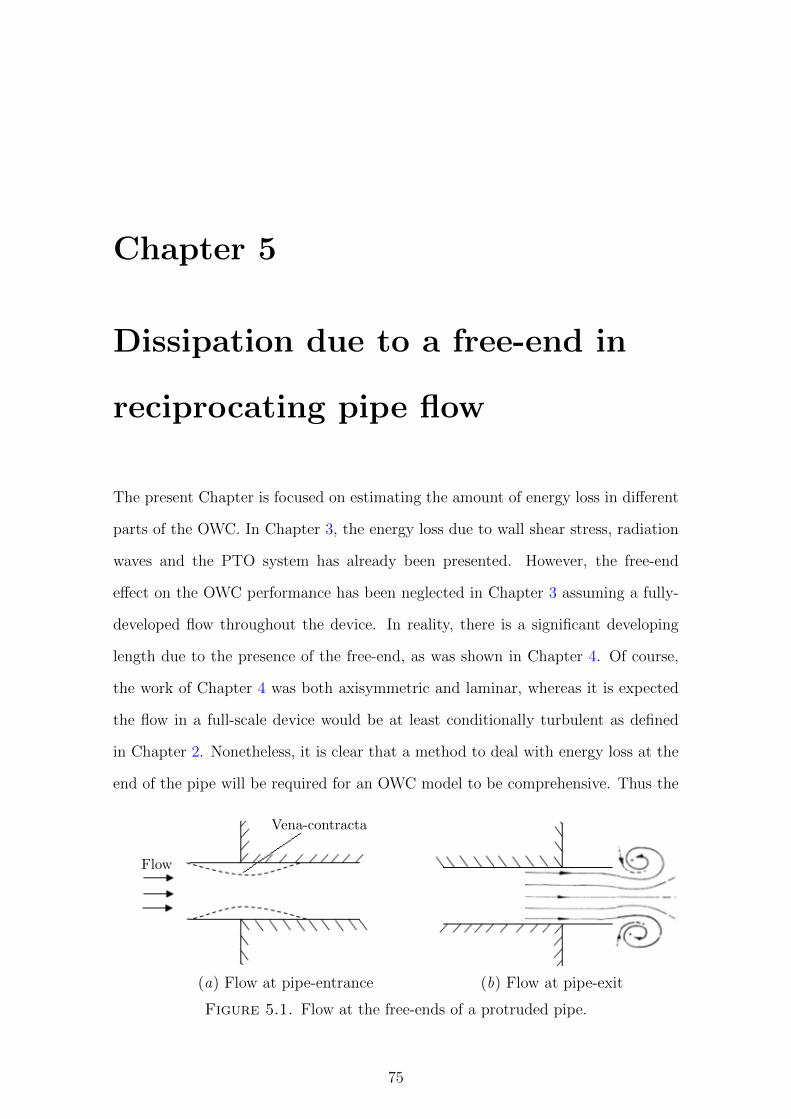
Chapter 5

Dissipation due to a free-end in

reciprocating pipe flow

The present Chapter is focused on estimating the amount of energy loss in different

parts of the OWC. In Chapter 3, the energy loss due to wall shear stress, radiation

waves and the PTO system has already been presented. However, the free-end

effect on the OWC performance has been neglected in Chapter 3 assuming a fully-

developed flow throughout the device. In reality, there is a significant developing

length due to the presence of the free-end, as was shown in Chapter 4. Of course,

the work of Chapter 4 was both axisymmetric and laminar, whereas it is expected

the flow in a full-scale device would be at least conditionally turbulent as defined

in Chapter 2. Nonetheless, it is clear that a method to deal with energy loss at the

end of the pipe will be required for an OWC model to be comprehensive. Thus the

Vena-contracta

Flow

(a) Flow at pipe-entrance (b) Flow at pipe-exit

Figure 5.1. Flow at the free-ends of a protruded pipe.

75

present Chapter deals with the energy loss due to the free-end in OWCs.

As the flow enters into the pipe through a sharp entrance, flow separation takes

place immediately after the entrance, resulting in the streamlines converging towards

the centre of the pipe. As the convergence reaches the maximum, the cross-sectional

area of the flow moving in the bulk direction becomes a minimum, which is known

as the “vena-contracta” as shown in Figure 5.1(a). Owing to continuity, for an

incompressible flow, the velocity increases and pressure decreases from the entrance

to the vena-contracta. However, from the vena-contracta to the end of the developing

region the streamlines diverge again, causing the velocity to decrease and pressure

to increase. Since the pressure gradient is favourable until the vena-contracta, loss

due to the separation is insignificant in this part. However, in the later part where

the streamlines expand, the pressure gradient is adverse; hence eddies are generated

and cause energy dissipation.

As the flow exits the pipe and enters into the reservoir, the stationary fluid in

the reservoir slows down the outer layer of the flow owing to viscosity, resulting the

formation of a vortex ring as shown in Figure 5.1(b). This vortex ring carries a

significant amount of kinetic energy, which eventually dissipates due to viscosity.

In a unidirectional pipe flow, one end of the pipe works as an entrance and the

other end works as an exit. Energy loss due to a sharp entrance or exit in this kind of

flow has been studied extensively. The loss coefficients determined from these studies

have been used in engineering problems for decades [75–77]. However, when the flow

is reciprocating, the free-ends of the pipe work as both the entrance and exit in one

complete cycle. Thus, the generation of the streamline convergence and its evolution

in one half of the cycle, and, during the other half of the cycle, the separation of

the boundary layer, causing the generation of eddies outside of the pipe, cause the

energy loss due to the free-end in reciprocating flow. Very few studies have been

conducted to measure the free-end losses in reciprocating pipe flow. Among these, it

was noted in Chapter 2 that Knott and Mackley in [11] conducted an experimental

study on the vortex formation at the mouth of a partially submerged vertical tube.

76

It was found that the separation takes place both during the inflow and the outflow.

The vortex generation and their dynamics have been analysed and presented in

detail. The cycle-average energy dissipation rate owing to the vortices generated at

the mouth and the wall shear stress were found as

˙Eew = 1.24ρAU30 , (5.1)

where ρ is the fluid density, A is the cross-sectional area and U0 is the amplitude of

the cross-sectional area averaged velocity. As noted in Chapter 2, a contemporary

experimental study by Knott and Flower [12] has shown that the total power loss

due to the wall shear stress inside the pipe and the vortices generated at the free-end

can be given by equation (2.11), repeated here as

˙Eew =1

2CU2

0 + 0.212KeρU30 , (5.2)

where C is a linear damping coefficient and Ke is the proportion of kinetic energy

being dissipated at the entrance. It has been assumed in [11] and [12] that the

linear damping term 12CU2

0 comes from the wall shear stress and radiation damping

as mentioned in Chapter 2, section 2.3.3; whereas the non-linear term 0.212KeρU30

comes from the vortices generated at the free-end.

In both [11] and [12] (mentioned above), the energy dissipation owing to the

wall shear stress and free-end was measured. Since the submergence depth of the

tubes in both these experimental studies was small, the contribution of the wall

shear stress loss to the overall loss was very small. Therefore, it was mentioned that

the measured loss of energy is due to the free-end only, though the total loss was

measured, which includes a contribution from both the wall shear stress and free-end

loss. These experiments were conducted for high Womersley number α = 12D√ω/ν

and for low area-average velocity amplitude A0 = U0/(ωD). The aim of the work

in this Chapter is to measure the wall shear stress and free-end losses separately in

reciprocating pipe flow and to quantify them for a range of α and A0. The direct

77

numerical simulation (DNS) code which has been used in Chapter 4 to measure

the developing length, is used in this Chapter to measure the energy loss. Since

the code works perfectly for the laminar flow (as validated in section 4.1 and as

will be validated again in this Chapter), the results presented here are confined

within the laminar regime. Of course, this means that only the results of Chapter

3 are applicable to a full-scale OWC in which the flow may be expected to include

conditional turbulence. However, the present Chapter introduces a methodology

applicable to any future numerical or experimental measurement, further improving

the ultimate OWC model.

5.1 Formulation

In this section, the dimensionless energy equation is derived, and applied to a specific

control volume which is used to measure the free-end loss in reciprocating pipe flow.

The integral form of the momentum conservation equation for an arbitrary con-

trol volume of volume V is

∫V

ρ∂ui∂t

dV +

∫V

ρuj∂ui∂xj

dV =

∫V

ρgi dV −∫V

∂p

∂xidV +

∫V

∂τij∂xj

dV. (5.3)

Multiplying equation (5.3) by ui, and applying continuity for incompressible flow,

i.e. ∂ui/∂xi = 0, to the resultant equation, gives the mechanical energy equation as

∫V

∂

∂t

(1

2ρu2

i

)dV +

∫V

∂

∂xj

(uj

1

2ρu2

i

)dV =

∫V

ρuigi dV −∫V

∂

∂xi(pui) dV

+

∫V

[∂

∂xj(τijui) dV − τij

∂ui∂xj

]dV. (5.4)

Applying Gauss’ theorem to equation (5.4) gives

∫V

∂

∂t

(1

2ρu2

i

)dV +

∫A

1

2ρu2

iuj dAj =

∫V

ρuigi dV −∫A

pui dAi

+

∫A

τijui dAj −∫V

τij∂ui∂xj

dV, (5.5)

78

where the subscript A indicates an integral over the domain surface, and the sub-

script V indicates an integral over the domain volume. The viscous shear stress, τij

for Newtonian incompressible fluids is connected to the strain as,

τij = 2µeij, (5.6)

where the strain eij is the symmetric part of the tensor ∂ui/∂xj, i.e.,

eij =1

2

(∂ui∂xj

+∂uj∂xi

).

The variables in energy equation are scaled as follows to obtain the dimensionless

equation,

x∗i =xiD, u∗i =

uiU0

, t∗ =tU0

Dand p∗ =

p

ρU20

,

where “ ∗ ” represents the non-dimensional variables, D is the pipe diameter, U0 is

the cross-sectional mean velocity amplitude and ρ is the fluid density. Introducing

the non-dimensional variables into equation (5.5) gives

ρU30D

2

∫V

∂

∂t∗

(1

2u∗i

2

)dV ∗ + ρU3

0D2

∫A

1

2u∗i

2u∗j dA∗j = ρU0D

3

∫V

u∗i gi dV∗

−ρU30D

2

∫A

p∗u∗i dA∗i + µU2

0D

∫A

2e∗iju∗i dA

∗j − µU2

0D

∫V

2e∗ije∗ij dV

∗. (5.7)

Dividing the above equation (5.7) by ρU30D

2 and removing the “∗”s give the dimen-

sionless energy equation as,

∫V

∂

∂t

(1

2u2i

)dV +

∫A

1

2u2iuj dAj =

DgiU2

0

∫V

ui dV −∫A

pui dAi

+1

4A0α2

∫A

2eijui dAj −1

4A0α2

∫V

2eijeij dV, (5.8)

where (as mentioned earlier) A0 = U0/ωD and α =D

2

√ω/ν; and ω is the oscillation

frequency.

Figure 5.2 shows the geometry that is used to investigate the energy loss. In it

79

Figure 5.2. Schematic diagram of the geometry.

a long pipe connects the two reservoirs, where the pipe-ends are extended into the

reservoirs. All the dimensions are scaled by the diameter of the pipe. A sinusoidal

volume flow rate is maintained at the inlet/outlet boundary to generate the recipro-

cating flow. Since the flow is being investigated in a horizontal pipe and the impact

of the weight of the fluid on the energy distribution is assumed negligible, the body

force can be considered to be zero, i.e., gi = 0.

A control volume marked by the dotted lines in Figure 5.3 is considered to

measure the loss in the pipe. On the control surfaces which are along the walls

the strain tensor eij 6= 0, however the velocity ui = 0 due to the no slip boundary

condition. Therefore at the walls, eijui = e.u = 0. Additionally, on the right-most

vertical control surface, a parallel flow is imposed; thus on this control surface the

radial component of the velocity, v = 0. On the left-most vertical control surface,

the flow is parallel owing to the fully developed condition; thus v = 0 on this control

surface as well. Hence, on these two control surfaces, eijui = e.u = 0. Therefore the

summation of eijui on all the control surfaces becomes zero, i.e.,∫Aeijui dAj = 0.

The energy equation for the control volume in Figure 5.3 can therefore be written

→↑ x

r

Figure 5.3. Control volume to investigate the free-end loss.

80

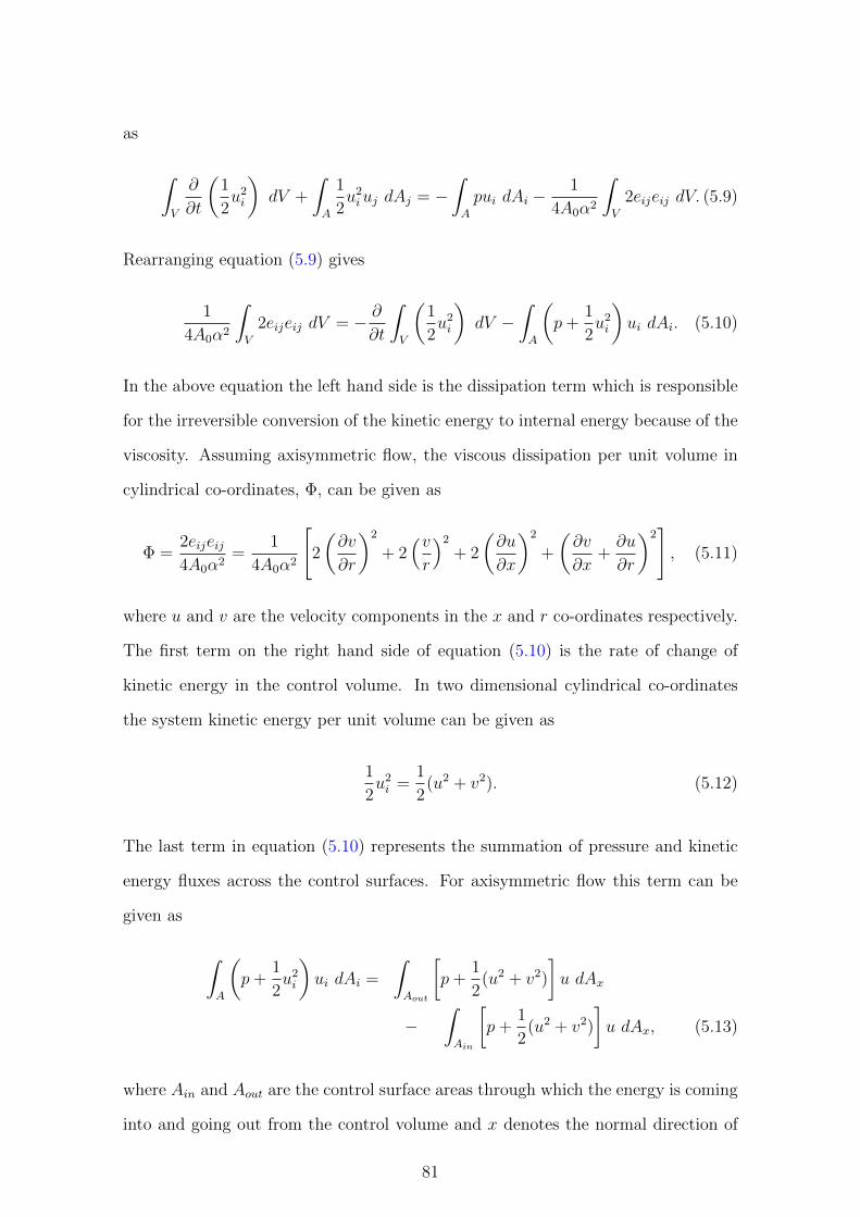
as

∫V

∂

∂t

(1

2u2i

)dV +

∫A

1

2u2iuj dAj = −

∫A

pui dAi −1

4A0α2

∫V

2eijeij dV. (5.9)

Rearranging equation (5.9) gives

1

4A0α2

∫V

2eijeij dV = − ∂

∂t

∫V

(1

2u2i

)dV −

∫A

(p+

1

2u2i

)ui dAi. (5.10)

In the above equation the left hand side is the dissipation term which is responsible

for the irreversible conversion of the kinetic energy to internal energy because of the

viscosity. Assuming axisymmetric flow, the viscous dissipation per unit volume in

cylindrical co-ordinates, Φ, can be given as

Φ =2eijeij4A0α2

=1

4A0α2

[2

(∂v

∂r

)2

+ 2(vr

)2

+ 2

(∂u

∂x

)2

+

(∂v

∂x+∂u

∂r

)2], (5.11)

where u and v are the velocity components in the x and r co-ordinates respectively.

The first term on the right hand side of equation (5.10) is the rate of change of

kinetic energy in the control volume. In two dimensional cylindrical co-ordinates

the system kinetic energy per unit volume can be given as

1

2u2i =

1

2(u2 + v2). (5.12)

The last term in equation (5.10) represents the summation of pressure and kinetic

energy fluxes across the control surfaces. For axisymmetric flow this term can be

given as

∫A

(p+

1

2u2i

)ui dAi =

∫Aout

[p+

1

2(u2 + v2)

]u dAx

−∫Ain

[p+

1

2(u2 + v2)

]u dAx, (5.13)

where Ain and Aout are the control surface areas through which the energy is coming

into and going out from the control volume and x denotes the normal direction of

81

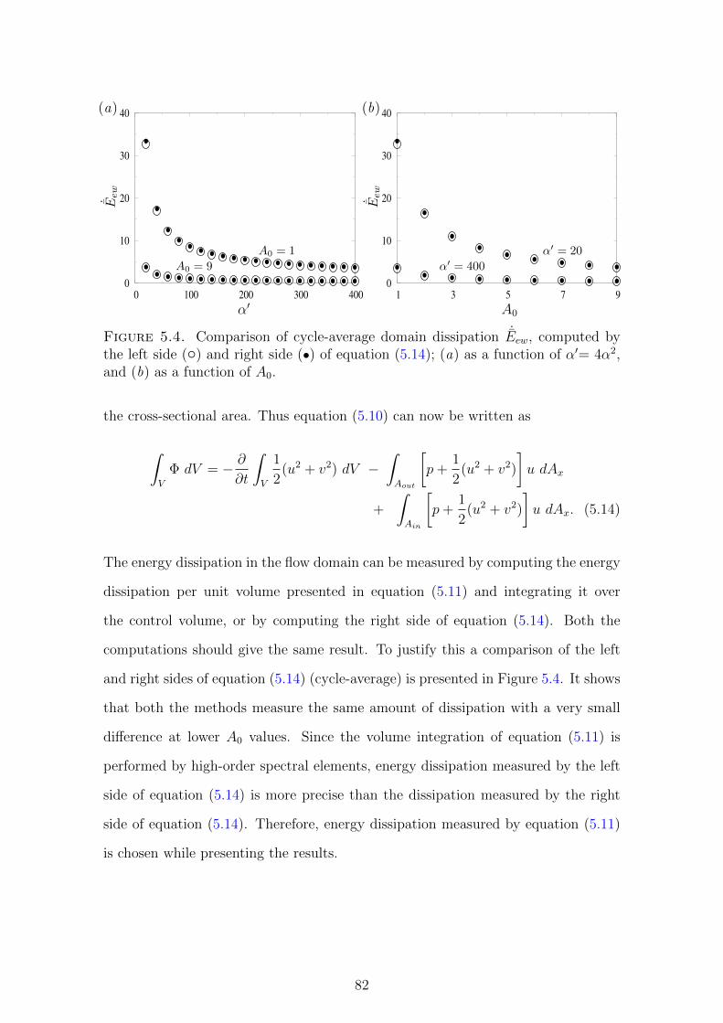
0

10

20

30

40

0 100 200 300 400

0

10

20

30

40

1 3 5 7 9

A0 = 9

A0 = 1

α′ = 400

α′ = 20

α′ A0

˙ Eew ˙ Eew

(a) (b)

Figure 5.4. Comparison of cycle-average domain dissipation ˙Eew, computed bythe left side (◦) and right side (•) of equation (5.14); (a) as a function of α′= 4α2,and (b) as a function of A0.

the cross-sectional area. Thus equation (5.10) can now be written as

∫V

Φ dV = − ∂

∂t

∫V

1

2(u2 + v2) dV −

∫Aout

[p+

1

2(u2 + v2)

]u dAx

+

∫Ain

[p+

1

2(u2 + v2)

]u dAx. (5.14)

The energy dissipation in the flow domain can be measured by computing the energy

dissipation per unit volume presented in equation (5.11) and integrating it over

the control volume, or by computing the right side of equation (5.14). Both the

computations should give the same result. To justify this a comparison of the left

and right sides of equation (5.14) (cycle-average) is presented in Figure 5.4. It shows

that both the methods measure the same amount of dissipation with a very small

difference at lower A0 values. Since the volume integration of equation (5.11) is

performed by high-order spectral elements, energy dissipation measured by the left

side of equation (5.14) is more precise than the dissipation measured by the right

side of equation (5.14). Therefore, energy dissipation measured by equation (5.11)

is chosen while presenting the results.

82

5.2 Validation

The DNS code described in Appendix C is validated by comparing the numerical

results with analytical results for cycle-average friction coefficient Cf (presented

below) and energy dissipation ˙Eew (defined next page) in the fully developed region.

The theoretical axial velocity gradient across the pipe,∂u

∂rfor a fully developed

reciprocating flow is obtained after a slight modification (to account for the pure

reciprocating case with a zero mean flow) of Uchida’s solution presented in [32].

Thus,∂u

∂rin the fully developed region of a laminar reciprocating pipe flow can be

given as

∂u

∂r=

4νA0α3

D√

(α− 2C1)2 + 4C22

bei(α)∂

∂rber(2αr)− ber(α)

∂

∂rbei(2αr)

ber2(α) + bei2(α)cos(ωt)

−ber(α)

∂

∂rber(2αr) + bei(α)

∂

∂rbei(2αr)

ber2(α) + bei2(α)sin(ωt)

, (5.15)

where

C1 =ber(α)

d

dαbei(α)− bei(α)

d

dαber(α)

ber2(α) + bei2(α), C2 =

ber(α)d

dαber(α) + bei(α)

d

dαbei(α)

ber2(α) + bei2(α);

where ‘ber’ and ‘bei’ are the Kelvin functions. Equation (5.15) is used to calculate

the analytical wall friction coefficient as,

Cf (t) =µ∂u

∂r

∣∣∣w

1

2ρU2

0

, (5.16)

and hence the cycle-average wall friction coefficient can be calculated as Cf =

1

T

∫ T

0

Cf (t)dt. Equation (5.15) is further used to calculate the dimensionless en-

ergy dissipation in the fully developed region as

Eew =

∫V

1

4A0α2

(∂u

∂r

)2

dV, (5.17)

83

0

0.05

0.1

0.15

0.2

0 100 200 300 400

0

0.05

0.1

0.15

0.2

0.25

0 100 200 300 400

α′ α′

Cf ˙ Eew

(a) (b)

Figure 5.5. Comparison between theoretical results (◦) and simulation results (•)of (a) wall friction coefficient Cf and (b) domain energy dissipation ˙Eew, as a functionof α′ = 4α2 for A0 = 3.

and hence the cycle-average dissipation as, ˙Eew =1

T

∫ T

0

Eew(t)dt.

While presenting the results, as in Chapter 4, α′ = 4α2 is used instead of α to

avoid fractional numbers. Comparison between the theoretical results and simula-

tion results are presented in Figure 5.5. It shows that for both the cycle-average

wall-friction coefficient Cf and the cycle-average energy dissipation ˙Eew, the DNS

code computes the exact values.

5.3 Results

As noted earlier, there are few works available in the literature which reported

experimental studies to investigate the free-end loss in reciprocating pipe flow i.e.,

[11, 12]. However in experiments, it is difficult to measure the wall shear stress

and the free-end losses separately. Thus the results presented in the previous works

are in fact the combination of both the losses. In the present work, an approach

is taken to present the wall shear stress loss and free-end loss individually, and

make a comparison between them. Loss of energy is presented for the entire flow

domain (Figure 5.3), for the wall shear stress inside the pipe and for the free-end.

Furthermore, the loss due to the vortices generated outside the pipe is also presented.

84

5.3.1 Energy loss in the entire domain, ˙Eew

Figure 5.6 shows the dimensionless cycle-average energy loss in the flow domain. It

includes the energy loss due to shear stress inside the pipe and the loss due to the

free-end; i.e., ˙Eew = ˙Ew + ˙Ee. The domain loss ˙Eew is presented as a function of α′

in (a), as a function of A0 in (b), as a function of 1/(A0α′) in (c) and as a function

of 1/(A0α′0.75) in (d). From (a), it can be seen that ˙Eew decreases with the increase

of α′ for different A0. The difference between ˙Eew values measured at different A0

also decreases with the increase of α′. Figure 5.6(b) shows that the same phenomena

happens when ˙Eew is plotted against A0 for different α′. Since the dimensionless

energy dissipation presented in equation (5.11) is a function of 1/(A0α′), ˙Eew is

0

4

8

12

0 100 200 300 400

A0 = 3 ×A0 = 5 •A0 = 9 ◦

0

3

6

9

1 3 5 7 9

α′ = 100 —×—α′ = 200 —•—α′ = 300 —◦—

α′ A0

˙ Eew ˙ Eew

(a) (b)

0

10

20

30

40

0 0.01 0.02 0.03 0.04 0.05

0

10

20

30

40

0 0.02 0.04 0.06 0.08 0.1 0.12

1/A0α′

˙ Eew

1/A0α′0.75

˙ Eew

(c) (d)

Figure 5.6. Cycle-average energy dissipation in the entire domain, ˙Eew; (a) as afunction of α′, (b) as a function of A0, (c) as a function of 1/(A0α

′) and (d) as afunction of 1/(A0α

′0.75). The straight dashed line in (d) represents the correlation˙Eew = 291.05/(A0α

′0.75) + 0.035.

85

plotted against 1/(A0α′) in (c). It shows that ˙Eew follows two different linear trends

with 1/(A0α′). However, all the ˙Eew values collapse to a single linear trend when

they are plotted as a function of 1/(A0α′0.75), as shown in (d). Hence, the correlation

between ˙Eew and 1/(A0α′0.75) can be given as ˙Eew = 291.05/(A0α

′0.75) + 0.035.

5.3.2 Energy loss due to a fully developed flow throughout

the pipe, ˙Ew

In this section, the energy loss due to the wall shear stress inside the pipe ˙Ew is

presented, assuming that the flow is fully developed throughout the pipe, i.e., there

is no free-end effect inside the pipe (which might be possible if the mouth of the

pipe is designed as a bell mouth). The dimensionless cycle-average shear stress

loss, ˙Ew, is plotted in Figure 5.7; as a function of α′ in (a), as a function of A0 in

(b), as a function of 1/(A0α′) in (c) and as a function of 1/(A0α

′0.75) in (d). The

percentage contribution of ˙Ew to the ˙Eew is plotted as a function of 1/(A0α′0.5) in

(e). From (a) and (b), it can be seen that ˙Ew decreases with the increase of both

α′ and A0. Like ˙Eew, ˙Ew follows two distinct linear trends with 1/(A0α′) as shown

in (c). However, (d) shows that all the data collapse to a single trend when ˙Ew is

plotted against 1/(A0α′0.75). Hence the correlation between ˙Ew and 1/(A0α

′0.75) can

be established as ˙Ew = 276.15/(A0α′0.75) + 0.02. Finally, (e) shows the contribution

of ˙Ew to the entire domain loss ˙Eew. At lower A0α′0.5, almost all the loss in the

domain is from ˙Ew. However, as A0α′0.5 increases, this domination of ˙Ew in the

domain loss decreases. As 1/(A0α′0.5) decreases below 0.05, the contribution of ˙Ew

drops drastically. Since the pipe is long, even after this rapid drop, the wall shear

stress loss ˙Ew still dominates at lower 1/(A0α′0.5) values.

5.3.3 Energy loss due to the free-end, ˙Ee

If it is assumed that the free-end does not have any effect on the flow (i.e., no

generation of vortices during inflow or outflow due to the free-end), then the total

loss of energy in the flow domain is due the shear stress loss inside the pipe only,

86

0

4

8

12

0 100 200 300 400

A0 = 3 ×A0 = 5 •A0 = 9 ◦

0

3

6

9

1 3 5 7 9

α′ = 100 —×—α′ = 200 —•—α′ = 300 —◦—

α′ A0

˙ Ew ˙ Ew

(a) (b)

0

10

20

30

40

0 0.01 0.02 0.03 0.04 0.05

0

10

20

30

40

0 0.02 0.04 0.06 0.08 0.1 0.12

1/A0α′

˙ Ew

1/A0α′0.75

˙ Ew

(c) (d)

80

85

90

95

100

0 0.05 0.1 0.15 0.2 0.25

˙ Ew/

˙ Eew

(%)

1/A0α′0.5

(e)

Figure 5.7. Cycle-average energy dissipation inside the pipe due to shear stress

assuming fully developed flow, ˙Ew; (a) as a function of α′, (b) as a function of A0, (c)as a function of 1/(A0α

′) and (d) as a function of 1/(A0α′0.75). (e) The percentage

contribution of ˙Ew in ˙Eew as a function of 1/(A0α′0.5). The straight dashed line in

(d) represents the correlation ˙Ew = 276.15/(A0α′0.75) + 0.02.

which were studied in Chapter 3, i.e., ˙Eew = ˙Ew. However, the inclusion of the

free-end effect in the system increases the overall loss in the domain; hence ˙Eew can

87

0.05

0.1

0.15

0.2

0.25

0 100 200 300 400

A0 = 3 ×A0 = 5 •A0 = 9 ◦

0.08

0.1

0.12

0.14

0.16

0.18

1 3 5 7 9

α′ = 100 —×—α′ = 200 —•—α′ = 300 —◦—

α′ A0

˙ Ee ˙ Ee

(a) (b)

0.05

0.1

0.15

0.2

0.25

0.3

0 0.01 0.02 0.03 0.04 0.05

0.05

0.1

0.15

0.2

0.25

0.3

0 0.01 0.02 0.03 0.04 0.05

1/A0α′

˙ Ee

1/A0.330 α′

˙ Ee

(c) (d)

0.05

0.1

0.15

0.2

0.25

0 0.01 0.02 0.03 0.04

1/A0.330 α′

0

5

10

15

20

0 0.05 0.1 0.15 0.2 0.25

1/A0α′0.5

(e) (f )

˙ Ee/

˙ Eew

(%)

˙ Ee

Figure 5.8. Cycle-average energy dissipation due to the free-end, ˙Ee; (a) as afunction of α′, (b) as a function of A0, (c) as a function of 1/(A0α

′), (d) as afunction of 1/(A0.33

0 α′) and (e) as a function of 1/(A0.330 α′) for A0 > 1. (f ) The

percentage contribution of ˙Ee in ˙Eew as a function of 1/(A0α′0.5). The dashed line

in (d) represents the correlation ˙Ee = 1/[1 + 1.16(A0.330 α′)0.33].

be expressed as ˙Eew = ˙Ew + ˙Ee, where ˙Ee is the loss due to the free-end. Values of

˙Eew and ˙Ew have been evaluated and already presented in section 5.3.2 and 5.3.4.

In this section the free-end loss ˙Ee is presented. It is evaluated by subtracting ˙Ew

88

from ˙Eew. Figure 5.8 shows the dimensionless cycle-average free-end loss ˙Ee, (a)

as a function of α′, (b) as a function of A0, (c) as a function of 1/(A0α′) and (d)

as a function of 1/(A0.330 α′). Figure 5.8(e) shows the same result as (d), however

excluding ˙Ee values for A0 = 1; these values were excluded because, as noted below,

A0 = 1 results differ from the trend for other A0 values. Finally, (f ) shows the

contribution of ˙Ee in the total domain loss ˙Eew as a function of 1/(A0α′0.5).

From (a) it can be seen that the ˙Ee decreases with the increase of α′ for different

A0. Figure 5.8(b) shows that at α′ = 100, ˙Ee remains nearly flat for the range of

2 ≤ A0 ≤ 7. However for α′ = 200 and 300, ˙Ee decreases with the increase of A0,

except for a little jump at A0 = 6 for α′ = 300. It is difficult to see any trend when

˙Ee is plotted against 1/(A0α′) as shown in (c). However (d) shows that ˙Ee follows a

trend if it is plotted against 1/(A0.330 α′). Thus an approximate correlation between

˙Ee and 1/(A0.330 α′) can be given as ˙Ee = 1/[1 + 1.16(A0.33

0 α′)0.33]. It also shows

that there are some values of ˙Ee that remain off the trend. It is found that these

off-trend data are the ˙Ee values at A0 = 1. Thus a new plot excluding the values for

A0 = 1 is presented in (e). The plot in (f ) shows that at higher 1/(A0α′0.5) values,

percentage of energy dissipation due to the free-end is small. However, with the

decrease of 1/(A0α′0.5), this contribution increases. As 1/(A0α

′0.5) decreases below

0.05, the percentage of ˙Ee increases drastically. Since the pipe is long, even though

the contribution of ˙Ee increases significantly, it reaches a maximum up to 20% of

the total energy loss.

5.3.4 Energy loss outside the pipe due to the free-end, ˙Eeo

As the flow exits the pipe, due to the velocity difference between the outer layer of

the flow and stationary fluid in the reservoir, vortex formation takes place outside

the pipe as shown in Figure 5.1(b). Owing to viscosity, these vortices eventually

dissipate energy. This section deals with the portion of ˙Ee which is due to the vortices

outside the pipe. Here this loss has been denoted as ˙Eeo. Figure 5.9 shows ˙Eeo as

a function of different variables. Figures 5.9(a) and (b) show that ˙Eeo decreases

89

0.05

0.1

0.15

0.2

0.25

0 100 200 300 400

A0 = 3 ×A0 = 5 •A0 = 9 ◦

0.05

0.1

0.15

0.2

1 3 5 7 9

α′ = 100 —×—α′ = 200 —•—α′ = 300 —◦—

α′ A0

˙ Eeo ˙ Eeo

(a) (b)

0.05

0.1

0.15

0.2

0.25

0.3

0 0.01 0.02 0.03 0.04 0.05

0.05

0.1

0.15

0.2

0.25

0.3

0 0.01 0.02 0.03 0.04 0.05

1/A0α′

˙ Eeo

1/A0.330 α′

˙ Eeo

(c) (d)

0

3

6

9

12

0 0.1 0.2 0.3 0.4

˙ Eeo/

˙ Eew

(%)

1/A0α′0.33

(e)

Figure 5.9. Cycle-average energy dissipation outside the pipe due to the free-end,˙Eeo; (a) as a function of α′, (b) as a function of A0, (c) as a function of 1/(A0α

′)and (d) as a function of 1/(A0.33

0 α′). (e) The percentage contribution of Eeo in˙Eew as a function of 1/(A0α

′0.33). The dashed line in (d) represents the correlation˙Eeo = 1/[1 + 0.74(A0.33

0 α′)0.45].

with the increase of α′ and A0. It is difficult to see a clear trend if ˙Eeo is plotted

against 1/(A0α′), as shown in (c). However, (d) shows that a trend can be found if

90

it is plotted as a function of 1/(A0.330 α′). The dashed line represents the correlation

between ˙Eeo and 1/(A0.330 α′) as, ˙Eeo = 1/[1 + 0.74(A0.33

0 α′)0.45]. From Figure 5.9(d)

it is apparent that this correlation works better at lower 1/(A0.330 α′) values than the

higher values. Figure 5.9(e) shows the percentage contribution of ˙Eeo in the total

dissipation ˙Eew as a function of 1/(A0α′0.33). It can be seen that the contribution of

˙Eeo increases with the increase of A0α′0.33. It means that with the increase of either

A0 or α′, the dissipation due to the vortices generated outside the pipe increases.

5.3.5 Vorticity and energy dissipation fields around the free-

end

To demonstrate how the free-end contributes to the energy loss in the reciprocating

flow system, the generation and evolution of vortices near the free-end and energy

dissipation due to them on a sectional plane are presented in Figure 5.10, for α′ = 400

and A0 = 3. It shows the contours of vorticity on the left and contours of energy

dissipation rate Φ on the right. Since the contours of vorticity are presented on

a sectional plane, the vortices near the upper wall is opposite in direction to the

vortices neat the lower wall. In Figure 5.10(left), red colour represents the positive

vortices and blue colour represents the negative vortices. It can be seen that as the

flow exits the pipe, the stationary fluid in the reservoir detaches the outer layer of

the fast moving fluid that comes out from the pipe, owing to the viscosity. At the

phase of φ = π/3, a small negative vortex ring is already formed at the tip of that

detached fluid. As more fluid comes out of the pipe, a bigger positive vortex ring is

formed and the initially formed small ring separates from the bigger one (φ = 2π/3).

With time, the bigger vortex ring propagates further away from the free-end, while

the negative smaller one remains close to the free-end (φ = π). As the flow alters

direction, the smaller vortex ring is pushed back into the pipe, however the bigger

ring continues its journey away from the free-end (φ = 4π/3). During the inflow,

owing to the sharp entrance, vortices are formed at the free-end, however with the

opposite direction to vortices that were generated during the outflow. The intensity

91

φ = π/3

2π/3

π

4π/3

5π/3

2π

Figure 5.10. Contours of vorticity (left) and energy dissipation (right) at the free-end, for α′ = 400 and A0 = 3, at various oscillation phases φ. Red and blue colourson the vorticity contour represent positive and negative vortices respectively.

92

of vortices keeps on increasing in the first few diameters of pipe length throughout

the inflow. However, all these negative inside vortices are pushed towards of the

free-end as the outflow starts (φ = 5π/3) and eventually they are driven out to

generate another set of vortex rings outside the pipe (φ = 2π).

From the dissipation fields (Figure 5.10 (right)) it can be seen that during the

outflow most of the dissipation inside the pipe takes place near the wall due to

the wall shear stress, and this dissipation is quite uniform throughout the pipe

(φ = π/3). Outside the pipe, most of the dissipation takes place due to the shear

between the stationary fluid in the reservoir and the moving fluid from the pipe.

Hence, the dissipation caused by the outside vortices is due to the shear between the

outer part of the vortices and reservoir fluid, and also due to the shear between the

fluid layers inside the vortices themselves. However, as the vortex ring propagates

further away from the free-end, it becomes weaker; thus the dissipation by the vortex

ring also decreases. In fact within a few diameters downstream from the free-end,

the vortices becomes so weak that the dissipation caused by the vortices becomes

insignificant. During the inflow (from φ = π to 5π/3), the flow separates from the

wall due to the sharp entrance, thus the dissipation takes place due to the shear

between fluid layers (a bit above the wall) but not in the actual wall shear layer. As

the flow crosses the “vena-contracta”, it gets attached to the wall and the dissipation

takes place due to the wall shear stress.

5.3.6 Comparison between ˙Ew and ˙Ee for different pipe

lengths

In the present work, the losses are investigated in a control volume which consists

a 50-diameter long pipe, as shown in Figure 5.3. It can be seen from Figure 5.10

that after a few diameters length from the free-end, dissipation due to the wall

shear stress is uniform. Due to this uniform dissipation, the amount of dissipation

increases linearly with the pipe length. Thus the result presented in Figure 5.7(e)

shows that ˙Ew is the dominating loss in the domain. However, the free-end loss

93

0

20

40

60

80

100

0 0.05 0.1 0.15 0.2

lc/D= 50

10

5

50

10

5

˙Ew •˙Ee ◦

˙ E/

˙ Eew

(%)

1/Reδ

Figure 5.11. Comparison between the contribution of dissipations from the wall

shear stress (assuming fully developed flow) ˙Ew and from the free-end ˙Ee to the

overall domain dissipation ˙Eew as a function of 1/Reδ for different pipe lengths.

remains constant regardless of the length of the pipe, hence ˙Ee is always less than

˙Ew (Figure 5.8(f )). While calculating ˙Ew it has been assumed that the flow is fully

developed throughout the pipe. On the same assumption, ˙Ew is computed for 10

and 5 diameters from the free-end and presented as a percentage of ˙Eew in Figure

5.11 along with the result for a 50-diameter long pipe. Results are presented as

a function of 1/Reδ, where Reδ = 2√

2A0α. On the same plot, the free-end loss

˙Ee in terms of the percentage of ˙Eew is presented for 50, 10 and 5 diameter long

pipes. While computing, it has been assumed that ˙Ee remains unaffected with the

change of the pipe length. This comparison shows that as the pipe gets shorter, the

contribution of the ˙Ee to the total loss ˙Eew increases. For a five-diameter long pipe,

the contribution of ˙Ee to the ˙Eew increases such an extent that as Reδ goes above

80, ˙Ee becomes the dominating loss in the domain. For many OWCs that have been

constructed, those discussed in Chapter 1, the equivalent of the “pipe” length to

diameter ratio is closer to five than to ten.

94

5.3.7 The total dissipation ˙Eew as a function of A0 at low

and high α′

Figure 5.12 shows ˙Eew as a function of A0 at α′ = 100, 200 and 3.57×104. Results for

α′ = 100 and 200 have been taken from the present study, whereas for α′ = 3.57×104

results have been taken from the experimental study presented in [12]. It can be

seen that ˙Eew shows a similar trend with A0 for both low and high α′ values. Like in

Figure 5.6(b), ˙Eew in Figure 5.12 decreases with both A0 and α′. However, though

there is a big jump in α′ (from 400 to 3.57 × 104), the difference in corresponding

˙Eew values is very small, specially for A0 > 0.8.

0

0.5

1

1.5

2

2.5

0.2 0.4 0.6 0.8 1 1.2 1.4

A0

˙ Eew

α′ = 100 —×—α′ = 400 —◦—

α′ = 3.57× 104 —•— [12]

Figure 5.12. Cycle-average total dissipation ˙Eew in a domain with a 2.3-diameterlong pipe (to match the length of the pipe of [12]), as a function of A0 at low α′

(from simulation) and at high α′ (from experiment [12]).

5.4 Summary

Entrance and exit losses in unidirectional pipe flow have been studied rigorously in

the literature and the evaluated loss coefficients are universally accepted. However,

in reciprocating pipe flow, the free-end loss has not been studied to the extent in

the literature that a correlation can be established between the loss and the flow

95

variables. Thus, in the present work an extensive study is conducted to investigate

the cycle-average losses in reciprocating pipe flow. A dimensionless energy equation

is derived for a control volume to evaluate the dissipation term, which is then used

to calculate the losses. Energy losses in different areas of the flow domain along with

the loss in the entire domain are measured. The cycle-average losses are presented

as a function of A0 = U0/ωD and α′ = 4α2. It is found that the dominant loss

is due to the shear stress in the pipe when the pipe is long. However if the pipe

gets shorter, the domination of the inside-pipe shear stress loss decreases and the

contribution of the free-end loss to the overall loss increases. It is found that if the

pipe is 5 diameters long, for Reδ = 2√

2A0α > 80, the free-end loss is more than the

inside-pipe shear stress loss. Additionally, the generation of the vortex rings during

the outflow and their dynamics have been visualised and explained. The energy loss

due to the vortices outside the pipe has also been measured and presented. Finally,

the energy loss measured in [12] has been plotted with the results from the present

study. It is found that the variation of the energy dissipation at α′ = 400 and

3.57×104 is very small for A0 > 0.8. Since a short pipe has been used (2.3 diameter

long) to measure the loss in [12], it can be assumed that the most of the loss is due

to the free-end. It can be anticipated that with the increase of α′ the free-end loss

would not change much. Thus, to estimate the free-end loss in the OWCs where

A0 > 0.8, results for α′ = 400 can be used.

A future work would be to use the same methodology to compute the losses in

conditionally turbulent flows.

96

Chapter 6

Analytical models of a tuned

Oscillating Water Column

In this chapter, the analytical models for a fixed-type tuned Oscillating Water Col-

umn (OWC) device are derived, incorporating the losses due to shear stress (viscous

and turbulent), radiation wave and the free-end. This is intended to be an example

illustrating one application of the research in the preceding chapters. It is expected

that the OWCs will resonate at the incident wave frequencies to ensure maximum

amount of power extraction. This is possible when the natural frequency of the

device coincides with the incident wave frequency. However, wave frequency varies

within a significant range. Therefore to maintain the resonance condition, it may

be beneficial to have a tuning mechanism which will adjust the natural frequency of

the device to the wave frequency. As mentioned in Chapter 2, section 2.2.2, several

tuning mechanisms have been proposed for fixed type OWCs, such as a variable

volume air compression chamber in a seawater pump [28] and the U-OWC device

[33]. The present work incorporates the idea of a variable volume air-compression

chamber as the tuning system in an OWC, which is shown in Figure 6.1. This

air-compression chamber divides the water column into two individual oscillating

masses (Figure 6.1(b)); hence two modes of oscillation are expected inside the de-

vice. The first mode of oscillation is like a pendulum, where both the water columns

97

Pressure controller

Turbine

(a) (b)

Figure 6.1. OWC with an air-compression chamber; (a) Schematic diagram, (b)Water (green) and air (grey) zones in the device.

and the trapped air oscillates as a whole body, and the second mode is like a spring

oscillation, where the air in the air-compression chamber works as a spring, allowing

the two water columns to oscillate against each other. Depending on the frequency

of the incident wave, the pressure of air in the air-compression chamber can be

changed by a pressure controller system, which will adjust the natural frequency of

the device by changing the water column lengths. Thus the device will continuously

resonate regardless of the outside condition.

The prime factor that determines the amount of power extraction from a res-

onating OWC is the dissipation in the system. For a highly damped oscillator the

power extraction would not be significantly greater at resonance than non-resonant

cases. In such situations, tuning the system frequency to the wave frequency is not

effective. Therefore identifying the damping sources and modelling them properly

to estimate the power output is one of the most important design prerequisites.

In this chapter, the viscous and turbulent shear stress, and the radiation damping

are incorporated in the equations of motion of the water columns from Chapter 3.

Furthermore, the damping at the device free-end, which is estimated from a direct

numerical simulation of reciprocating pipe flow in Chapter 5, is incorporated into the

equations of motion. The equation for the power take-off (PTO) system is derived

98

in the same manner as the equation for the PTO system of a single water column

device, which has been derived in Chapter 3.

6.1 Formulation

If the instantaneous vertical displacement of the water column from its equilibrium

position is ξ, the equation of motion for a single water column in a fixed OWC can

be expressed, as in section 3.1, as,

(m+ αrd)ξ + βξ + ρwgSξ + fPTO = fd, (6.1)

where m is the mass of the water column, αrd is the added mass due to water outside

the mouth that is also set into motion, β is the damping coefficient, ρw is the water

density, g is the acceleration due to gravity, S is the free surface area of the water

column, fPTO is the force due to the PTO system and fd is the driving force from the

incident waves. The damping coefficient β in equation (6.1) represents the radiation

damping (βrd, due to the waves radiating outward from the device), the wall shear

stress damping (βtb and βlm) and the free-end damping (βfe).

Here, a mass-spring-damping model (equation 6.1) for each water column of the

tuned OWC is derived from the governing fluid dynamics equations that includes βrd,

βtb and βfe. For convenience, the variables in the mass and momentum conservation

equations are scaled to get the dimensionless equations.

The lengths in the cylindrical co-ordinate system, x∗i = (x∗, r∗, φ) are scaled as

follows,

x∗i = Dxi,

where “*” represents dimensional quantities and D is the diameter of the device.

Time, velocity and pressure are scaled with the bar representing the mean flow,

99

while primes represent fluctuating variables as follows,

t∗ = ω−1t,

u∗i = ωD(Ui + u′i

), (6.2)

p∗ = ρwgD(p+ p′),

ρ∗ = ρwρ,

where ω is the incident wave frequency and the velocity components are defined as

u∗i = (u∗, v∗, w∗).

6.1.1 Mass and momentum conservation equations for the

water columns

After scaling and ensemble averaging, the mass and momentum conservation equa-

tions for the incompressible flow in the water columns can respectively be written

as,

∇jUj = 0, (6.3)

∂Ui∂t

+ Uj∇jUi = − g

ω2D∇ip+

1

Reω

(∇2j Ui)−∇ju′iu

′j +

giω2D

, (6.4)

where the kinetic Reynolds number, Reω = ρwωD2/µ = 4α2; and α is the Wom-

ersley number. The derivation of equations (6.3) and (6.4) from the Navier-Stokes

equations are presented in Appendix A.1.1.

6.1.2 Simplifying the x-momentum equation of the water

columns

It is assumed that the flow in the water columns are axisymmetric (i.e., ∂()/∂φ =

0) and fully developed (i.e., ∂()/∂x = 0). Applying these assumptions in the x-

component of equation (6.4) (different components of the momentum equation for

100

the water zones are given in equations (A.14-A.16)) gives the x-momentum equation

as

∂U

∂t= − g

ω2D

∂p

∂x+

1

Reω

[1

r

∂

∂r

(r∂U

∂r

)]− 1

r

∂

∂r

(ru′v′

)+

gxω2D

. (6.5)

Following the definition of total shear stress presented in section 3.1.1, the total

shear stress in the water columns can be given as

τ =1

Reω

∂U

∂r− u′v′.

Introducing τ into equation (6.5) and averaging over the cross-sectional area gives

(detail are presented in section 3.1.1),

ξ = − g

ω2D

∂p

∂x− 4τw +

gxω2D

, (6.6)

where ξ is the normalised instantaneous displacement of the free surface inside the

device and τw is the dimensionless wall shear stress.

ξ0

ξ1lc0 h1

h2

h3

la0 la1ξ1

Figure 6.2. Dimensions of the OWC device.

101

6.1.3 Equation of motion for the water columns

Integration of equation (6.6) with respect to x along the first water column length

removes the spatial dependence of p and gives,

ξ0 = − 1

Klc0(pd − pc)− 4τw −

1

Klc0ξ0, (6.7)

where K = ω2/g, lc0 is the length of the first water column and ξ0 is the normalised

surface displacement of the column as shown in Figure 6.2. Figure 6.2 also shows

that the pressure at point d is pd, which is the air pressure in the air-compression

chamber and pc is the pressure at the OWC free-end.

Integration of equation (6.6) with respect to x along the second water column

length gives,

ξ1 = − 1

Klc1(ph − pe)− 4τw −

2

Klc1ξ1, (6.8)

where lc1 is the length of the second water column i.e. lc1 = h1 + h2 + h3, and ξ1 is

the normalised free surface displacement of the column as shown in Figure 6.2. In

equation (6.8), ph represents the air pressure in the plenum chamber (air chamber

below the turbine) and pe represents the air pressure in the air-compression chamber.

6.1.4 Modelling the pressure in the air-compression cham-

ber, pd and pe

The first water column in the OWC oscillates with the frequency of the incident

wave. Consequently, the air in the air-compression chamber oscillates approximately

at the same frequency. Since the wave frequency is quite low in the Ocean and the

sound speed is high in the air, the fluid properties in the air-compression cham-

ber barely change with space. It enables the assumption that the pressure in the

air-compression chamber is uniformly distributed, i.e. pd = pe. The spatial inde-

pendence of the pressure field allows treatment of the trapped air as an air-bubble.

102

Additionally, the heat generation and heat transfer due to the compression and ex-

pansion of the air can be considered negligible, hence it can be assumed that these

compression and expansion processes are adiabatic. Thus assuming air as an ideal

gas, the relationship between the pressure and volume can be given as

pgVγ = constant, (6.9)

where pd = pe = pg is the pressure in the air-compression chamber, V is the volume

of the air-compression chamber and γ is the adiabatic index. Equation (6.9) can be

expressed as

pgVγ = pg0V

γ0 ,

pg =pg0V

γ0

V γ, (6.10)

where pg0 and V0 are respectively the tuning pressure and volume of the air-compression

chamber, i.e. pressure and volume of the air-compression chamber before the oscil-

lation starts. The dimensionless volume of the air-compression chamber before the

oscillation starts (V0) and after the oscillation (V ) can respectively be given as

V0 =π

4

(la0

D

)and V =

π

4

(la0 −Dξ0 +Dξ1

D

).

Thus,

pg =pg0l

γa0

(la0 −Dξ0 +Dξ1)γ. (6.11)

It is assumed that the pressure fluctuation in the air-compression chamber is small,

which enables linearization of pg with respect to ξ0 and ξ1. Thus, taking the first-

order derivatives after the Taylor series expansion of pg(ξ0, ξ1) (details are presented

103

in Appendix A.2) gives,

pg(ξ0, ξ1) = pg0 +γDpg0la0

ξ0 −γDpg0la0

ξ1. (6.12)

6.1.5 Modelling the entrance pressure, pc

The pressure at the OWC free-end pc is composed of the pressure from the incident

wave that drives the water column pf , and the pressure induced by the radiation

wave pr. Thus the equation of motion for the first water column (equation (6.7))

can be written as

ξ0 + 4τw +1

Klc0ξ0 +

1

Klc0pg =

1

Klc0(pf + pr). (6.13)

The entire flow field of the OWC can be split into a rotational and an irrotational

flow field. The driving pressure pf , and the pressure due to radiation wave pr are

derived from the irrotational flow. Additionally, pf is modelled considering that

there is no power take-off (PTO) system. Thus the only factor that would cause

the air in the air-compression chamber to compress or expand is the inertia of the

second water column. However while modelling pf , it is assumed that the inertia

of the second water column is small, thus it oscillates along with the trapped air

and the first water column. The pressure due to the radiation wave, pr, is modelled

considering that there is no incident wave. Thus, while modelling pr it is assumed

that the resistance from the first water column and the surrounding water to the

wave that radiates away from the device (due to the pressure fluctuation in the

plenum chamber) is small. Hence the water columns and the trapped air oscillate as a

solid body during radiation. For simplicity, both pf and pr are modelled considering

that the interaction between the waves and the complex geometry of the device is

the same as the interaction between the waves and a simple device presented in

Chapter 3.

Following the above assumptions, the derivation of pf and pr would be the same

104

as for a simple device (Chapter 3), which is provided in Appendix B. However in

the Appendix, pf is expressed as pd. Thus the absolute value of the amplitude of

the driving pressure (pf ) can be presented as

|Pf | =√

2hsN1/20 |q∗s |

πkD3sinh(kh)

∣∣∣∣∣ B

B2 + A2+ i

A

B2 + A2

∣∣∣∣∣ , (6.14)

where k = 2π/λ is the wave number, h is the water depth,

N0 = 0.5(1 + (sinh(2kh)/2kh)), q∗s is the induced volume flux due to scattered

waves, hs is the significant wave height and, A and B are the radiation susceptance

and radiation conductance respectively. Detailed definitions of these parameters are

given in Appendix B.2. The pressure due to the radiation wave (pr) can be expressed

as

pr = −Klc0(βrdξ0 + αrdξ0), (6.15)

where αrd is the added mass and βrd is the radiation damping. Thus the equation

of motion for the first water column after substituting equation (6.14) and (6.15) in

equation (6.13) can be given as

(1 + αrd)ξ0 + βrdξ0 + 4τw +1

Klc0ξ0 +

1

Klc0pg =

1

Klc0pf . (6.16)

6.1.6 Including the damping due to the free-end of the OWC

Energy loss due to the free-end in reciprocating pipe flow has been measured and

presented in Chapter 5. The free-end loss was computed by subtracting the wall

shear stress loss inside the pipe from the total energy loss in the domain, i.e., ˙Ee =

˙Eew − ˙Ew. While calculating the wall shear stress loss inside the pipe ( ˙Ew), it was

assumed that the flow is fully developed throughout the pipe. In the present study,

the equation of motion for the first water column which is derived in equation (6.16)

also assumes that the flow is fully developed throughout the pipe. Now if the free-

end loss measured in Chapter 5 can be interpreted as a damping term and added

to equation (6.16), then all the possible losses that the first water column may

105

experience would be included into the equation of motion.

Since the velocity in Chapter 5 has been scaled by U0 and in the present Chapter

it is scaled by ωD, a conversion is required to incorporate the free-end loss ˙Ee into

equation (6.16). The conversion is done as follows,

˙E∗ep =(ρwπ

4D2lc0 + α∗rd

)ξ∗e0ξ

∗0 = ρwω

3D5

(πlc04D

)(1 + αrd)ξe0ξ0

= ˙Ee5 × ρwU30D

2, (6.17)

where ˙E∗ep is the free-end loss, ξe0 is the additional acceleration of the first water

column due to the free-end and ˙Ee5 is the free-end loss scaled by the variables of

Chapter 5. Hence ξe0 can be interpreted as a damping term as follows,

(1 + αrd)ξe0 =4D ˙Ee5ρwU

30D

2

πlc0ρwω3D5|ξ0|2 ξ =

4D ˙Ee5A30

πlc0|ξ0|2 ξ0 = βfeξ0; (6.18)

thus the damping coefficient due to the free-end is given by βfe =4D ˙Ee5A

30

πlc0|ξ0|2 . Intro-

ducing the free-end damping into equation (6.16) gives,

(1 + αrd)ξ0 + (βrd + βfe)ξ0 + 4τw +1

Klc0ξ0 +

1

Klc0pg =

1

Klc0pf . (6.19)

6.1.7 Modelling the wall shear stress, τw in the reciprocating

flow system of the OWC

The presence of the boundary layers creates the rotational flow field in the OWC.

The shear stress term, τw in the equation of motion represents the boundary layers

and is derived in a similar manner to the way it was derived for a single water

column device in section 3.1.2.

As mentioned in section 3.1.2, the flow in the OWC is either turbulent or condi-

tionally turbulent, i.e. laminar during the acceleration phases and turbulent during

the deceleration phases. For the turbulent portion of the cycle, τw in section 3.1.2.1

106

was derived as

τw =1

4βtbξ, (6.20)

where βtb = 0.15816 Re−1/4ω |ξ|3/4. Substituting equation (6.20) into (6.19) gives the

equation of motion for the first water column including turbulent wall shear stress

damping as

(1 + αrd) ξ0 + (βrd + βfe + βtb) ξ0 +1

Klc0ξ0 +

1

Klc0pg =

1

Klc0pf ; (6.21)

and substituting equation (6.20) into (6.8) gives the equation of motion for the

second water column including turbulent wall shear stress damping as

ξ1 + βtbξ1 +2

Klc1ξ1 +

1

Klc1ph =

1

Klc1pg, (6.22)

For the laminar portion of the cycle, τw in section 3.1.2.1 was derived as

τw =1

4(αlmξ + βlmξ), (6.23)

where αlm = 32Fωsin θ1, βlm = 32Fωcos θ1; and θ1 is the phase difference and the

factor Fω is given by

Fω =

√C2

1 + C22

16√

(α− 2C21)2 + 4C2

2

(6.24)

where C1 and C2 are constants and α =√

Reω/2. Substituting equation (6.23) into

equation (6.19) gives the governing equation of motion for the first water column

including laminar wall shear stress damping as

(1 + αrd + αlm) ξ0 + (βrd + βfe + βlm) ξ0 +1

Klc0ξ0 +

1

Klc0pg =

1

Klc0pf ; (6.25)

and substituting equation (6.23) into (6.8) gives the equation of motion for the

second water column including laminar wall shear stress damping as

(1 + αlm)ξ1 + βlmξ1 +2

Klc1ξ1 +

1

Klc1ph =

1

Klc1pg. (6.26)

107

6.1.8 Modelling the Power-Take-Off (PTO)

The PTO of the present OWC device is modelled in exactly the same manner as

the PTO of the single device was modelled in section 3.1.3. Thus the dimensionless

equation for the air pressure in the plenum chamber can be given as

dphdt

+ 4c2Ktd0

πla1Nt

ph = KD2ρac2

la1

ξ1, (6.27)

where c is the dimensionless sound speed, Nt is the dimensionless turbine rotational

speed, d0 is the turbine rotor diameter, la1 is the length of the plenum chamber and

Kt is an empirical turbine coefficient which is fixed for a given turbine geometry.

Furthermore, as mentioned earlier, K = ω2/g and D is the OWC diameter.

6.1.9 Summary of the governing equations

For convenience, the governing equations derived for the OWC are summarised

below.

The equations of motion for the first and second water columns in the turbulent

portion of the cycle are respectively,

(1 + αrd) ξ0 + (βrd + βfe + βtb) ξ0 +1

Klc0ξ0 +

1

Klc0pg =

1

Klc0pf , (6.28)

and

ξ1 + βtbξ1 +2

Klc1ξ1 +

1

Klc1ph =

1

Klc1pg. (6.29)

The equations of motion for the first and second water columns in the laminar

portion of the cycle are respectively,

(1 + αrd + αlm) ξ0 + (βrd + βfe + βlm) ξ0 +1

Klc0ξ0 +

1

Klc0pg =

1

Klc0pf , (6.30)

108

and

(1 + αlm)ξ1 + βlmξ1 +2

Klc1ξ1 +

1

Klc1ph =

1

Klc1pg. (6.31)

The air pressure in the air-compression chamber is given by

pg = pg0 +γDpg0la0

ξ0 −γDpg0la0

ξ1. (6.32)

The equation for the PTO system is

dphdt

+ 4c2Ktd0

πla1Nt

ph = KD2ρac2

la1

ξ1. (6.33)

6.2 Results

The dimensionless instantaneous power output is calculated as

P =p∗a

ρwgD× Q∗

ωD3=π

4paξ, (6.34)

and the dimensionless average power as

Pavg =1

T

∫ T

0

P (t)dt, (6.35)

where the wave period, T = 2π/ω.

The value of Pavg is computed, first for the radiation damping, second for the

radiation and turbulent damping, and finally for the radiation, turbulent and free-

end damping by solving equations (6.28), (6.29), (6.32) and (6.33). The explicit

fourth order Runge-Kutta algorithm is used to solve them numerically.

The equations are solved for the first water column length to water depth ratio

lc0/h = 0.4, second water column to water depth ratio lc1/h = 1.2, diameter to

water depth ratio D/h = 0.1, the air-compression chamber length to water depth

ratio la0/h = 0.3, the plenum chamber length to water depth ratio la1/h = 0.6,

109

0

0.1

0.2

0.3

0.4

0.5

0.6

1 1.5 2 2.5 3

Kh

Pavg

Figure 6.3. Average dimensionless power against dimensionless parameter Kh fordifferent damping : —, radiation (βrd); —, radiation and turbulent (βrd + βtb) and—, radiation, turbulent and free-end (βrd + βtb + βfe).

the significant wave height to water depth ratio hs/h = 0.2, turbine parameter

Ktd0/(la1N∗t ) = 0.00064 s, and the specific heat ratio for air γ = 1.4. During

the computation, it is considered that the pressure in the air-compression chamber

pg0 = 1. As it has been seen from Chapter 5, Figure 5.12, that the energy dissipation

rates due to the free-end (i.e. ˙Ee values) for Reω = 400 do not vary significantly

from the ˙Ee values for Reω = 3.57× 104, ˙Ee values for Reω = 400 has been used to

compute the free-end damping coefficient βfe.

Figure 6.3 shows the power output from the OWC, Pavg, as a function of Kh

for different damping. Two different modes (as mentioned in the beginning of this

Chapter), the pendulum mode and the spring-like mode are apparent from the

Figure. It can be seen that the resonance for the pendulum mode occurs at Kh =

1.723, and for the spring-like mode the resonance occurs at Kh = 2.576. It also

shows that the inclusion of free-end damping reduces the power output significantly.

110

6.3 Summary

Two equations of motion for the two water columns in a tuned OWC have been

derived from the Navier-Stokes equations. The pressures at the OWC free-end (due

to the incident and radiation waves) and in the plenum chamber (due to the PTO

system) have been modelled in a similar manner as they were modelled for the

OWC in Chapter 3. Additionally, the pressure due to the adiabatic compression

and expansion of air in the air-compression chamber has been linearized assuming

that the pressure fluctuation in the chamber is small. The free-end damping has

been incorporated into the equations of motion from Chapter 5. The governing

equations have been solved for different damping models to calculate the power

extraction by the device. As expected, two resonances were noticed for the two

modes of oscillation; one for the pendulum mode of oscillation and the other one

for the spring-like oscillation. It has been found that the inclusion of the free-end

damping reduces the power output significantly.

Since the present Chapter was focused on illustrating how the work of the pre-

ceding Chapters might be applied to future technology developments, a detailed

study on the tuning mechanism was left as a future work. Thus, a future study is

suggested to investigate the pressure and volume in the air-compression chamber to

tune the device with the incident wave frequency.

111

Chapter 7

Conclusion

A mass-spring-damping model of a single-column fixed-type near-shore OWC has

been derived from the Navier-Stokes equations. Damping due to the wall shear

stress during the laminar and turbulent portions of the cycle has been incorporated

respectively from [32] and [9]. Damping due to the radiation wave has been calcu-

lated from [1] and incorporated into the current model through a conversion process

presented in [30]. While modelling the PTO system, it has been assumed that the air

in the air chamber compresses and expands isentropically. The flow inside the OWC

has been assumed fully developed throughout the device, neglecting the free-end

effect.

It has been found that wider devices encounter most of their damping from

radiation waves. However, as the device gets narrower, the wall shear stress damping

becomes significant at the resonance. Thus for better efficiency, the wall shear stress

damping needs to be considered while designing a resonant OWC. Additionally, it

has been shown as expected, that the overall power extraction by the device increases

with the increase of the significant wave height. Furthermore, it has been shown in

Figure 3.11 that with the increase of significant wave height, the device can extract

significant amount of power over wider range of wave frequency.

As a requirement of evaluating whether the flow in an OWC is fully developed

throughout the device, an extensive Direct Numerical Simulation (DNS) study has

been conducted to investigate the developing length in a reciprocating pipe flow.

112

The centreline velocity, uc and the radial gradient of the x-direction velocity at the

wall, ∂u/∂r|w have been used to measure the developing length.

It has been found that the developing length follows a sinusoidal pattern over

the cycle, making a 90◦ phase difference with the centreline velocity uc. It has

been shown that if the maximum developing length (le)max and the cycle-average

developing length (le)mean are scaled by the Stokes-layer thickness δ and plotted

against Reδ, the following linear correlations are possible.

For the maximum entrance length the correlation is

(le)max/δ = 1.37Reδ + 5.3,

valid for the range of modified Womersley number α′ from 100 to 300 for the am-

plitude A0 such that 1 ≤ A0 ≤ 9 and from 300 to 400 for 1 ≤ A0 ≤ 7.

For the cycle-average entrance length the correlation is

(le)mean/δ = 0.82Reδ + 2.16,

valid for the range of α′ from 150 to 300 for 1 ≤ A0 ≤ 9 and from 300 to 400 for

1 ≤ A0 ≤ 7.

Hence, it has become clear that the developing length at the OWC free-end

is significant. Thus, an approach has been taken to measure the free-end loss in

reciprocating pipe flow which includes the energy loss in the developing region. A

dimensionless energy equation has been derived for a control volume to evaluate

the dissipation term, which then has been used to calculate the losses. The rate

of energy dissipation in different areas of the flow domain have been measured. It

has been found that the maximum proportion of loss is due to the internal shear

stress when the pipe is long. However, as the pipe gets shorter, the domination

of the inside-pipe shear stress loss decreases and the contribution of the free-end

loss to the overall loss increases. It has been found that if the pipe is 5 diameters

long, for Reδ = 2√

2A0α > 80, the free-end loss is more than the inside-pipe shear

113

stress loss. Additionally, visualisation of the vortices and the energy dissipation

field showed that the vortices get weaker as they propagate away from the free-end,

and within few diameters downstream energy dissipation caused by those vortices

becomes insignificant. Furthermore, a comparison between the energy loss measured

in [12] and the results from the present DNS study showed that the variation of the

energy dissipation at α′ = 400 and 3.57 × 104 is very small for A0 > 0.8. Thus, to

estimate the free-end loss in the OWCs where A0 > 0.8, results for α′ = 400 can be

used.

Finally, the governing equations for a tuned OWC have been derived, incorpo-

rating the free-end damping along with the wall shear stress and radiation damping.

Since this is intended to be only an illustration of an application of the preceding

results, a detailed study on the tuning mechanism was beyond the scope of present

study. Therefore, a future study is suggested to investigate the pressure and volume

in the air-compression chamber in order to tune the device with the incident wave

frequency. However, it has been found that the inclusion of the free-end damping

reduces the power output significantly.

114

Appendices

115

Appendix A

Dimensionless governing equations

for OWC

A.1 Reynolds-Averaged Navier-Stokes (RANS) equa-

tions

The differential form of the mass conservation or the continuity equation is

∂ρ∗

∂t∗+∇∗j(ρ∗u∗j) = 0 (A.1)

and the momentum conservation equation is

∂(ρ∗u∗i )

∂t∗+∇∗j(ρ∗u∗iu∗j) = −∇∗i p∗ +∇∗jτ ∗ij + ρ∗gi, (A.2)

where τ ∗ij is the viscous stress tensor and “∗ ” denotes dimensional variables. For an

isotropic fluid, the viscous stress,

τ ∗ij = λ¯e∗ij + 2µe∗ij,

116

where

e∗ij =1

2

(∂u∗i∂x∗j

+∂u∗j∂x∗i− 2

3

∂u∗k∂x∗k

δij

)=

1

2

(∇∗ju∗i +∇∗iu∗j −

2

3∇∗ku∗kδij

)

and

¯e∗ =1

3

∂u∗k∂x∗k

δij =1

3∇∗ku∗kδij.

Here µ(T ) is the dynamic viscosity, λ(T ) is the second viscosity which is usually

neglected, and δij is the Kronecker delta function. Thus τ ∗ij can be written as,

τ ∗ij = µ

(∂u∗i∂x∗j

+∂u∗j∂x∗i− 2

3

∂u∗k∂x∗k

δij

)= µ

(∇∗ju∗i +∇∗iu∗j −

2

3∇∗ku∗kδij

)(A.3)

The lengths in the cylindrical co-ordinate system, x∗i = (x∗, r∗, φ) are scaled as

follows,

x∗i = Dxi,

where “*” represents dimensional quantities and D is the diameter of the device.

Time, velocity and pressure are scaled with the bar representing the mean flow,

while primes represent fluctuating variables as follows,

t∗ = ω−1t,

u∗i = ωD(Ui + u′i

), (A.4)

p∗ = ρwgD(p+ p′),

ρ∗ = ρwρ.

where ω is the incident wave frequency and the velocity components are defined as

u∗i = (u∗, v∗, w∗). Thsu the continuity equation can be written as

∂ρ

∂t+∇j[ρ(Uj + u′j)] = 0. (A.5)

Ensemble average of (A.5) will eliminate the term containing single fluctuating quan-

117

tity i.e., u′j. Thus after the ensemble average, equation (A.5) can be given as,

∂ρ

∂t+∇j(ρUj) = 0. (A.6)

In cylindrical co-ordinate system,

∇j =∂

∂x~ex +

∂

∂r~er +

1

r

∂

∂φ~eφ.

Applying (A.3) to (A.2) gives the momentum equation as

∂(ρ∗u∗i )

∂t∗+∇∗j(ρ∗u∗iu∗j) = −∇∗i p∗ +∇∗j{µ(∇∗ju∗i +∇∗iu∗j −

2

3∇∗ku∗kδij)}+ ρ∗gi. (A.7)

There is no change of dynamic viscosity µ in the OWC, thus

∂(ρ∗u∗i )

∂t∗︸ ︷︷ ︸(1)

+∇∗j(ρ∗u∗iu∗j)︸ ︷︷ ︸(2)

= −∇∗i p∗︸ ︷︷ ︸(3)

+µ∇∗j(∇∗ju∗i +∇∗iu∗j −2

3∇∗ku∗kδij)︸ ︷︷ ︸

(4)

+ ρ∗gi︸︷︷︸(5)

. (A.8)

Introducing the scaling from equation (A.4) to the term (1) of (A.8) is

∂(ρ∗u∗i )

∂t∗= ρwDω

2 ∂

∂t(ρUi + ρu′i).

After ensemble averaging,

∂(ρ∗u∗i )

∂t∗= ρwDω

2 ∂

∂t(ρUi),

Ensemble averaged value of term (2) after scaling is

∇∗j(ρ∗u∗iu∗j) = ρwDω2 ∇j[ρUiUj + ρ(u′iu

′j)].

Ensemble averaged value of term (3) after scaling is

∇∗i p∗ = ρwg∇iP .

118

Ensemble averaged value of term (4) after scaling is

µ∇∗j(∇∗ju∗i +∇∗iu∗j −2

3∇∗ku∗kδij) =

ωµ

D∇j(∇jUi +∇iUj −

2

3∇kUkδij).

Ensemble averaged value of term (5) after scaling is

ρ∗gi = ρwρgi.

Thus, the ensemble average of equation (A.8) after scaling can be written as

∂

∂t(ρUi) + ∇j

[ρUiUj + ρ(u′iu

′j)]

= − gi

ω2D∇iP

+1

Reω∇j

(∇jUi +∇iUj −

2

3∇kUkδij

)+

ρgiω2D

(A.9)

where the kinetic Reynolds number Reω = 4α2; α =D

2

√ρwω

µis the Womersley

number.

A.1.1 RANS equations for the water column in OWC

In the water column, the normalised density ρ = 1. Thus, the continuity equation

(A.6) in the water column is

∇jUj = 0, (A.10)

where Uj = (U , V , W ). Therefore,

∂U

∂x+

1

r

∂(rV )

∂r+

1

r

∂W

∂φ= 0. (A.11)

The momentum equation (A.9) becomes,

∂Ui∂t

+ ∇j

[UiUj + u′iu

′j

]= − gi

ω2D∇iP

+1

Reω∇j

(∇jUi +∇iUj −

2

3∇kUkδij

)+

giω2D

,

119

∂Ui∂t

+[Uj∇jUi + Ui∇jUj +∇j(u′iu

′j)]

= − gi

ω2D∇iP

+1

Reω

(∇2j Ui +∇i∇jUj −

2

3∇j∇kUkδij

)+

giω2D

. (A.12)

Applying (A.10) to (A.12) gives,

∂Ui∂t

+ Uj∇jUi = − gi

ω2D∇iP +

1

Reω∇2j Ui −∇j(u′iu

′j) +

giω2D

. (A.13)

The x-component of equation (A.13) is

∂U

∂t+

[U∂U

∂x+ V

∂U

∂r+W

r

∂U

∂φ

]= − gx

ω2D

∂P

∂x

+1

Reω

[∂2U

∂x2+

1

r

∂

∂r

(r∂U

∂r

)+

1

r2

∂2U

∂φ2

]

−

[∂u′2

∂x+

1

r

∂

∂r

(ru′v′

)+

1

r

∂(u′w′)

∂φ

]+

gxω2D

. (A.14)

The r-component of equation (A.13) is

∂V

∂t+

[U∂V

∂x+ V

∂V

∂r+W

r

∂V

∂φ− W 2

r

]= − gr

ω2D

∂P

∂r

+1

Reω

[∂2V

∂x2+

1

r

∂

∂r

(r∂V

∂r

)+

1

r2

∂2V

∂φ2− 2

r2

∂W

∂φ− V

r2

]

−

[∂(u′v′)

∂x+

1

r

∂(rv′2)

∂r+

1

r

∂(v′w′)

∂φ− w′2

r

]+

grω2D

. (A.15)

120

The φ-component of equation (A.13) is

∂W

∂t+

[U∂W

∂x+ V

∂W

∂r+W

r

∂W

∂φ+V W

r

]= − gφ

ω2D

1

r

∂P

∂φ

+1

Reω

[∂2W

∂x2+

1

r

∂

∂r

(r∂W

∂r

)+

1

r2

∂2W

∂φ2+

2

r2

∂V

∂φ− W

r2

]

−

[∂(u′w′)

∂x+

1

r

∂(rv′w′)

∂r+

1

r

∂w′2

∂φ+v′w′

r

]+

gφω2D

. (A.16)

A.1.2 RANS equations for the air-compression chamber

The air in the air-compression chamber is considered as a compressible gas. Thus,

substituting ρ in equation (A.6) by the air density ρa gives the continuity equation

for air-compression chamber as

∂ρa∂t

+∇j(ρaUj) = 0, (A.17)

∂ρa∂t

+

[∂

∂x(ρaU) +

1

r

∂

∂r(rρaV ) +

1

r

∂

∂φ(ρaW )

]= 0. (A.18)

The momentum equation for the air-compression chamber can be derived from equa-

tion (A.9) as

∂

∂t

(ρaUi

)+ ∇j

[ρaUiUj + ρa(u′iu

′j)]

= − gi

ω2D∇iP

+1

Reω∇j

(∇jUi +∇iUj −

2

3∇kUkδij

)+ρagiω2D

,

Ui∂ρa∂t

+ ρa∂Ui∂t

+ Ui∇j(ρaUj) + (ρaUj)∇jUi +∇j[ρa(u′iu′j)] = − gi

ω2D∇iP

+1

Reω∇j

(∇jUi +∇iUj −

2

3∇kUkδij

)+ρagiω2D

,

121

Ui

[∂ρa∂t

+∇j(ρaUj)

]+ρa

∂Ui∂t

+ (ρaUj)∇jUi +∇j[ρa(u′iu′j)]

= − gi

ω2D∇iP +

1

Reω∇j

(∇jUi +∇iUj −

2

3∇kUkδij

)+ρagiω2D

. (A.19)

Applying (A.17) to (A.19) gives,

ρa∂Ui∂t

+ ρaUj∇jUi +∇j[ρa(u′iu′j)]

= − gi

ω2D∇iP +

1

Reω∇j

(∇jUi +∇iUj −

2

3∇kUkδij

)+ρagiω2D

. (A.20)

The x-component of equation (A.20) is

ρa∂U

∂t+ ρa

[U∂U

∂x+ V

∂U

∂r+W

r

∂U

∂φ

]

= − gxω2D

∂P

∂x+

1

Reω

[∂τxx∂x

+1

r

∂(rτxr)

∂r+

1

r

∂τxφ∂φ

]

−ρa

[∂u′2

∂x+

1

r

∂

∂r

(ru′v′

)+

1

r

∂(u′w′)

∂φ

]+ρagxω2D

. (A.21)

The r-component of equation (A.20) is

ρa∂V

∂t+ ρa

[U∂V

∂x+ V

∂V

∂r+W

r

∂V

∂φ− W 2

r

]

= − grω2D

∂P

∂r+

1

Reω

[∂τxr∂x

+1

r

∂(rτrr)

∂r+

1

r

∂τrφ∂φ− τφφ

r

]

−ρa

[∂(u′v′)

∂x+

1

r

∂(rv′2)

∂r+

1

r

∂(v′w′)

∂φ− w′2

r

]+ρagrω2D

. (A.22)

122

The φ-component of (A.20) is

ρa∂W

∂t+ ρa

[U∂W

∂x+ V

∂W

∂r+W

r

∂W

∂φ+V W

r

]

= − gφω2D

1

r

∂P

∂φ+

1

Reω

[∂τxφ∂x

+1

r

∂(rτrφ)

∂r+

1

r

∂τφφ∂φ

+τrφr

]

−ρa

[∂(u′w′)

∂x+

1

r

∂(rv′w′)

∂r+

1

r

∂w′2

∂φ+v′w′

r

]+ρagφω2D

. (A.23)

123

A.1.3 Dimensionless shear stress tensor, τij in cylindrical

coordinate system

Different components of the dimensionless shear stress tensor in cylindrical coordi-

nate system can be given as

τxr =

[∂V

∂x+∂U

∂r

]

τxφ =

[∂W

∂x+

1

r

∂U

∂φ

]

τrφ =

[∂W

∂r+

1

r

∂V

∂φ− W

r

]

τxx = 2∂U

∂x− 2

3

[∂U

∂x+

1

r

∂(rV )

∂r+

1

r

∂W

∂φ

]

=4

3

∂U

∂x− 2

3

1

r

∂(rV )

∂r− 2

3

1

r

∂W

∂φ

τrr = 2∂V

∂r− 2

3

[∂U

∂x+V

r+∂V

∂r+

1

r

∂W

∂φ

]

=4

3

∂V

∂r− 2

3

V

r− 2

3

∂U

∂x− 2

3

1

r

∂W

∂φ

τφφ = 2

[1

r

∂W

∂φ+V

r

]− 2

3

[∂U

∂x+V

r+∂V

∂r+

1

r

∂W

∂φ

]

=4

3

1

r

∂W

∂φ+

4

3

V

r− 2

3

∂U

∂x− 2

3

∂V

∂r.

(A.24)

124

A.2 Linearizing the pressure in the air-compression

chamber, pg

Applying multi-variable taylor series expantion to pg with respect to ξ0 and ξ1 and

considering the first order derivatives only, gives

pg(ξ0, ξ1) = pg|0,0 + ξ0dpgdξ0

|0,0 + ξ1dpgdξ1

|0,0. (A.25)

Here

pg|ξ0,ξ1 =pg0l

γa0

(la0 −Dξ0 +Dξ1)γ,

pg|0,0 = pg0.

dpgdξ0

|ξ0,ξ1 = γDpg0l

γa0

(la0 −Dξ0 +Dξ1)γ+1 ,

dpgdξ0

|0,0 =γDpg0la0

.

dpgdξ1

|ξ0,ξ1 = −γD pg0lγa0

(la0 −Dξ0 +Dξ1)γ+1 ,

dpgdξ1

|0,0 = −γDpg0la0

.

Thus equation (A.25) can be written as

pg(ξ0, ξ1) = pg0 +γDpg0la0

ξ0 −γDpg0la0

ξ1. (A.26)

125

Appendix B

Modelling the pressure from the

incident and radiative waves, pd(t)

and pr(t)

The driving pressure pd(t) is generally modelled by solving the scattering of the in-

cident wave, in the absence of the pressure fluctuation in the air-chamber (i.e. when

pa(t) = 0). The radiation induced pressure pr(t) is modelled by solving for the radi-

ation wave, generated by the pressure oscillation in the air-chamber in the absence

of the incident wave. In the present work, we incorporated from [1] the derivation

of the internal volume fluxes (q∗s and q∗r), induced in the scattering and radiation

problems in a cylindrical OWC. In [1], hydrodynamic characteristics were derived by

considering an oscillating pressure distribution over the internal free surface. How-

ever, the aim here is to come up with a mechanical mass-spring-damping equivalent

model of the OWC (including shear stress damping). Such models are commonly

used to describe the oscillation of the rigid bodies in heave [78]. If the wavelengths

are not too short, it is possible to transform the hydrodynamic parameters of the

pressure-distribution model (i.e. [1]) to the rigid-body model (mass-spring-damping

model), as shown in [30]. A similar approach is taken to derive the pd(t) and pr(t)

of the current model from the induced internal volume fluxes q∗s(t) and q∗r(t) of [1].

126

B.1 Computing q∗s and q∗r from [1]

The time-dependent volume flux across an internal free surface of an OWC is defined

as, Q∗(t∗) = Re { q∗e−iωt∗}. The flux amplitude is

q∗ = q∗s +1

ρwg

dp∗adt∗

q∗r , (B.1)

where q∗s and q∗r are the induced volume fluxes in the scattering and radiation prob-

lems, respectively.

Under the assumptions of linear water-wave theory, solving for the velocity po-

tentials in different regions of the flow domain, gives

q∗s =4πikRhJ1(kR)S21

γH1(kR) + 2iS22

. (B.2)

Here the wavenumber, k = 2π/λ, γ = πkRkhJ1(kR) and R is the radius of the

device, J1 and H1 are the Bessel and Hankel functions of the first kind, respectively

and S12 and S22 are the elements of a 2×2 real symmetric matrix, S = {Sij}, which

expresses the hydrodynamic characteristics of the device. Following [25], the volume

flux due to the radiation is decomposed as

1

ρwg

dp∗adt∗

q∗r = −B∗p∗a −A∗

ω

dp∗adt∗

, (B.3)

where A∗ and B∗ are real, and following [79], these are called the radiation suscep-

tance and radiation conductance, respectively. Solving the radiation potential in

different regions of the flow domain gives the volume flux due to the radiation as,

q∗r =2πR(γH1(kR)S11 + 2i∆)

K[γH1(kR) + 2iS22], (B.4)

where ∆ = S11S22 − S12S21.

A Galerkin method is used to determine the matrix Sij, and hence q∗s and q∗r are

computed from equations (B.2) and (B.4).

127

B.2 Deriving the driving pressure, pd(t) and the

radiation induced pressure, pr(t) from q∗s and

q∗r

Following [30], q∗s and q∗r of the pressure-distribution model are transformed to the

pd(t) and pr(t) of the current mass-spring-damping model. The q∗s and q∗r in section

(B.1) are derived based on potential flow theory. Therefore, to incorporate them into

our model, we need to have an equation of motion that separates the irrotational

wave physics outside the OWC and in the far field, which can be represented by

potential flow, from the vorticity-dominated physics of the boundary layers inside

the OWC. To make it convenient, we split the internal flow field into the irrotational

and the rotational flow field. In this section, we first derive the pd(t) and pr(t) from

q∗s and q∗r for the irrotational flow. Then the shear stress term is added to the

equation of motion as a representative of the rotational flow inside the device. A

similar approach was presented in [28] while studying a wave-driven seawater pump.

Thus for the potential flow, equation (3.10) can be written as

ξ +1

Klcξ +

1

Klcpa =

1

Klc(pd + pr). (B.5)

The induced force due to the radiation wave can be expressed as

1

Klcpr = −Zrξ, (B.6)

where Zr is called the radiation impedance [80]. The oscillation in the OWC is

assumed to be time-harmonic with the incident-wave frequency ω; thus the time-

dependent displacement and pressures can be expressed by,

{ξ, pd, pr, pa}(t) = Re({D, Pd, Pr, Pa

}e−it), (B.7)

128

where D, Pd, Pr and Pa are the amplitudes. Equation (B.5) can be rewritten as

1

Klcpa =

1

Klcpd −

(Zr + i

1

Klc− i)ξ. (B.8)

The net volume flux across the internal free surface, Q∗ = ωDSξ, where S is the

internal free surface area. Thus from equation (B.8),

Q∗

ωDS=

1

Klc

(pd − pa)(Zr + i

1

Klc− i) . (B.9)

Substituting (B.3) into (B.1) and scaling the resultant by equation (A.4) gives,

q∗

ωDS=

q∗sωDS

− Y Pa, (B.10)

where Y =ρwg

ωS(B∗ − iA∗) = B − iA. Equation (B.9) then becomes

q∗sωDS

− Y Pa =1

Klc

(Pd − Pa)(Zr + i

1

Klc− i) . (B.11)

By definition, q∗s is the volume flux across the internal free surface when Pa = 0,

thus from equation (B.11),

q∗sωDS

=1

Klc

Pd(Zr + i

1

Klc− i) ; (B.12)

therefore,

Y =1

Klc

1(Zr + i

1

Klc− i) . (B.13)

Rearrangement of equation (B.13), and the substitution of Y by A and B gives

Zr =1

Klc

B

B2 + A2+ i

(1

Klc

A

B2 + A2− 1

Klc+ 1

). (B.14)

129

Following [1], scaling the induced volume flux due to the scattering potential |q∗|, by

the volume flux across the internal free surface due to a solid mass of fluid oscillating

with the incident wave frequency ω and amplitude a gives,

|q∗s |ωaS

=4N

1/20 |q∗s |

πkD2sinh(kh), (B.15)

where N0 =1

2

(1 +

sinh(2kh)

2kh

). As shown in [81], the wave amplitude a of a

sinusoidal wave can linearly be related to the significant wave height as

a =hs

2√

2. (B.16)

Thus, substituting equations (B.14),(B.15) and (B.16) into (B.12) gives the absolute

value of the driving pressure amplitude

|Pd| =√

2hsN1/20 |q∗s |

πkD3sinh(kh)

∣∣∣∣∣ B

B2 + A2+ i

A

B2 + A2

∣∣∣∣∣ . (B.17)

Following [79], by analogy with electric-circuit theory, the radiation impedance Zr

is composed of the radiation resistance and radiation reactance. However, in hy-

drodynamics they are known as the radiation damping βrd(ω) and the added mass

αrd(ω), respectively, hence

Zr = βrd − iαrd. (B.18)

From equations (B.14) and (B.18), the dimensionless added mass is

αrd =1

Klc− 1

Klc

A

B2 + A2− 1, (B.19)

and radiation damping is

βrd =1

Klc

B

B2 + A2. (B.20)

130

Substituting equation (B.18) into (B.6) gives

1

Klcpr = −(βrd − iαrd)ξ = −βrdξ − αrdξ. (B.21)

131

Appendix C

Direct Numerical Simulation

(DNS) code description

The DNS code solves the Navier-Stokes equations for incompressible flow,

∇ · u = 0, (C.1)

∂u

∂t= −(u · ∇)u−∇P +

1

Re(∇2u). (C.2)

Equation (C.2) is solved by a 3-way time-splitting method. In this method each of

the three terms on the right side of equation (C.2) is integrated over one time-step

separately, using the result from the previous sub-step as the initial condition, i.e.,

u∗ − un = −∫ t+∆t

t

(u · ∇)u dt, (C.3)

u∗∗ − u∗ = −∫ t+∆t

t

∇P dt, (C.4)

un+1 − u∗∗ =1

Re

∫ t+∆t

t

∇2u dt, (C.5)

where n represents the current time-step, and u∗ and u∗∗ are intermediate velocity

fields at the end of the advection and pressure sub-steps, respectively.

Equation (C.3) is solved for u∗ using Adams-Bashforth scheme, which is a third-

order explicit method. The pressure P is solved first by taking the divergence of

132

equation (C.4), which gives

∇ · u∗∗ −∇ · u∗

∆t= −∇2P. (C.6)

Then continuity is enforced at the end of the step, i.e., ∇ · u∗∗ = 0; thus equation

(C.6) becomes,

∇2P =∇ · u∗

∆t, (C.7)

which is a Poisson equation. Now equation (C.7) is solved to calculate the pressure

P , which is then used in equation (C.4) to get u∗∗. This u∗∗ is then used in equation

(C.5) to calculate un+1 using a Crank-Nicolson scheme, which is a second-order

implicit method.

The spatial discretisation is done using a nodal-based spectral-element method.

This method is a member of the broader class of methods of weighted residuals. It

solves the equations of motion (C.5), (C.6) and (C.7) in the weak form or variational

formulation. The weak form requires the solution to be represented by a series of

functions, here the Lagrange polynomials are used. The weak form also requires

the evaluation of a series of integrals over the spatial domain which is efficiently

done by using internal points on each element that coincide with Gauss-Lobatto-

Legengre quadrature points. A thorough description of the spectral element method,

as applied to the Navier-Stokes equations, can be found in [82].

In the spectral-element method, the mesh can be refined by increasing the num-

ber of elements which is known as h-refinement and by increasing the number of

internal points (i.e. increasing the order of Lagrange polynomials) which is known

as p-refinement. In this thesis, a mesh using 5136 quadrilateral elements was used

with 8th order polynomials resulting in 64 internal points on each element.

133

References

[1] David V Evans and Richard Porter. Efficient calculation of hydrodynamic

properties of owc-type devices. Journal of Offshore Mechanics and Arctic En-

gineering, 119(4):210–218, 1997.

[2] TV Heath. A review of oscillating water columns. Philosophical Transac-

tions of the Royal Society A: Mathematical, Physical and Engineering Sciences,

370(1959):235–245, 2012.

[3] Ramiro Godoy-Diana and Steven PR Czitrom. On the tuning of a wave-energy

driven oscillating-water-column seawater pump to polychromatic waves. Ocean

Engineering, 34(17):2374–2384, 2007.

[4] Arturo Olvera, Esteban Prado, and Steven Czitrom. Parametric resonance in

an oscillating water column. Journal of Engineering Mathematics, 57(1):1–21,

2007.

[5] Paolo Boccotti. Comparison between a u-owc and a conventional owc. Ocean

Engineering, 34(5):799–805, 2007.

[6] SI Sergeev. Fluid oscillations in pipes at moderate reynolds numbers. Fluid

dynamics, 1(1):121–122, 1966.

[7] Mikio Hino, Masaki Sawamoto, and Shuji Takasu. Experiments on transition to

turbulence in an oscillatory pipe flow. Journal of Fluid Mechanics, 75(02):193–

207, 1976.

134

[8] David M Eckmann and James B Grotberg. Experiments on transition to turbu-

lence in oscillatory pipe flow. Journal of Fluid Mechanics, 222:329–350, 1991.

[9] R Akhavan, RD Kamm, and AH Shapiro. An investigation of transition to

turbulence in bounded oscillatory stokes flows part 1. experiments. Journal of

Fluid Mechanics, 225(1):395–422, 1991.

[10] JH Gerrard and MD Hughes. The flow due to an oscillating piston in a cylindri-

cal tube: a comparison between experiment and a simple entrance flow theory.

Journal of Fluid Mechanics, 50(01):97–106, 1971.

[11] GF Knott and MR Mackley. On eddy motions near plates and ducts, induced by

water waves and periodic flows. Philosophical Transactions of the Royal Society

of London. Series A, Mathematical and Physical Sciences, pages 599–623, 1980.

[12] GF Knott and JO Flower. Measurement of energy losses in oscillatory flow

through a pipe exit. Applied Ocean Research, 2(4):155–164, 1980.

[13] Ibrahim Dincer. Renewable energy and sustainable development: a crucial

review. Renewable and Sustainable Energy Reviews, 4(2):157–175, 2000.

[14] Antonio F de O Falcao. Wave energy utilization: A review of the technologies.

Renewable and sustainable energy reviews, 14(3):899–918, 2010.

[15] Alain Clement, Pat McCullen, Antonio Falcao, Antonio Fiorentino, Fred Gard-

ner, Karin Hammarlund, George Lemonis, Tony Lewis, Kim Nielsen, Simona

Petroncini, et al. Wave energy in europe: current status and perspectives.

Renewable and Sustainable Energy Reviews, 6(5):405–431, 2002.

[16] Sam Behrens, Jennifer Hayward, Mark Hemer, and Peter Osman. Assessing

the wave energy converter potential for australian coastal regions. Renewable

Energy, 43:210–217, 2012.

[17] NN Panicker. Power resource potential of ocean surface waves. In Proceedings

135

of the wave and salinity gradient workshop, Newark, Delaware, USA, pages

J1–J48, 1976.

[18] Stephen Barstow, Gunnar Mrk, Denis Mollison, and Joo Cruz. The wave en-

ergy resource. In Joao Cruz, editor, Ocean Wave Energy, Green Energy and

Technology(Virtual Series), pages 93–132. Springer Berlin Heidelberg, 2008.

[19] Michael E McCormick. Ocean wave energy conversion. New York, Wiley-

Interscience, 1981. 255 p., 1, 1981.

[20] Voith group. Energy from active breakwaters. http://www.voith.com, 2006.

[Online; last accessed 16-November-2016].

[21] Nancy Stauffer. Catch the wave. http://news.mit.edu, 2008. [Online; last

accessed 16-November-2016].

[22] Oceanlinx. Oceanlinx built and deployed an instrumented 1/3rd scale test unit

of its Mk2 WEC in late 2007 and early 2008. http://www.oceanlinx.com,

2007. [Online; last accessed 16-November-2016].

[23] N Johnson and E Olson. Oscillating Water Column (OWC). http://

owcwaveenergy.weebly.com, 2010. [Online; last accessed 16-November-2016].

[24] K Budal and J Falnes. Optimum operation of improved wave-power converter.

Mar. Sci. Commun.;(United States), 3(2), 1977.

[25] DV Evans. Wave-power absorption by systems of oscillating surface pressure

distributions. Journal of Fluid Mechanics, 114(1):481–499, 1982.

[26] AJNA Sarmento and AF de O Falcao. Wave generation by an oscillating surface-

pressure and its application in wave-energy extraction. Journal of Fluid Me-

chanics, 150:467–85, 1985.

[27] Alan Fleming, Irene Penesis, Gregor Macfarlane, Neil Bose, and Tom Denniss.

Energy balance analysis for an oscillating water column wave energy converter.

Ocean Engineering, 54:26–33, 2012.

136

[28] SPR Czitrom, R Godoy, E Prado, P Perez, and R Peralta-Fabi. Hydrodynamics

of an oscillating water column seawater pump: Part i: theoretical aspects.

Ocean engineering, 27(11):1181–1198, 2000.

[29] TS Zhao and P Cheng. The friction coefficient of a fully developed laminar

reciprocating flow in a circular pipe. International journal of heat and fluid

flow, 17(2):167–172, 1996.

[30] A Brendmo, J Falnes, and PM Lillebekken. Linear modelling of oscillating water

columns including viscous loss. Applied ocean research, 18(2):65–75, 1996.

[31] LMC Gato and AF de O Falcao. On the theory of the wells turbine. Journal

of engineering for gas turbines and power, 106(3):628–633, 1984.

[32] Shigeo Uchida. The pulsating viscous flow superposed on the steady laminar

motion of incompressible fluid in a circular pipe. Zeitschrift fur angewandte

Mathematik und Physik ZAMP, 7(5):403–422, 1956.

[33] Felice Arena, Vincenzo Fiamma, Valentina Laface, Giovanni Malara, Alessan-

dra Romolo, Antonino Viviano, Gianmaria Sannino, and Adriana Carillo. In-

stalling u-owc devices along italian coasts. In ASME 2013 32nd International

Conference on Ocean, Offshore and Arctic Engineering, pages V008T09A061–

V008T09A061. American Society of Mechanical Engineers, 2013.

[34] D Ross. Power from sea waves. Oxford University Press, United Kingdom,

1995.

[35] TJT Whittaker, SJ McIwaine, and S Raghunathan. A review of the islay

shoreline wave power station. In Proceedings of (First) European Wave Energy

Symposium, pages 283–6, 1993.

[36] H Ohneda, S Igarashi, O Shinbo, S Sekihara, K Suzuki, H Kubota, H Ogino, and

H Morita. Construction procedure of a wave power extracting caisson break-

water. In Tokyo: Proceedings of 3rd Symposium on Ocean Energy Utilization,

pages 171–9, 1991.

137

[37] Y Washio, H Osawa, Y Nagata, F Fujii, H Furuyama, and T Fujita. The offshore

floating type wave power device mighty whale: open sea tests. In Proceedings

of the 10th international offshore and polar engineering conference, volume 1,

pages 373–380, 2000.

[38] Pico OWC. OWC Pico power plant. http://www.pico-owc.net, 1999. [Online;

last accessed 16-November-2016].

[39] R Alcorn, S Hunter, C Signorelli, R Obeyesekera, T Finnigan, and T Denniss.

Results of the testing of the energetech wave energy plant at port kembla.

Energeth Report, 2005.

[40] Y Masuda, H Kimura, X Liang, X Gao, RM Mogensen, and T Andersen. Re-

garding bbdb wave power generation plant. In Proceedings of 2nd European

Wave Power Conference, pages 69–76, 1995.

[41] Ocean Energy. Ocean Energy-a world of power. http://www.oceanenergy.ie,

2011. [Online; last accessed 16-November-2016].

[42] Y Torre-Enciso, I Ortubia, LI Lopez de Aguileta, and J Marques. Mutriku

wave power plant: from the thinking out to the reality. In Proceedings of the

8th European Wave and Tidal Energy Conference, pages 319–329, 2009.

[43] Korea Research Institute of Ships and Ocean Engineering. Ocean energy policy.

https://report2014.ocean-energy-systems.org.

[44] Felice Arena, Alessandra Romolo, Giovanni Malara, and Alfredo Ascanelli. A

new u-owc device to produce electrical power from ocean waves: Some applica-

tions to italian coasts. 2014.

[45] DV Evans. The oscillating water column wave-energy device. IMA Journal of

Applied Mathematics, 22(4):423–433, 1978.

[46] JN Newman. Interaction of water waves with two closely spaced vertical ob-

stacles. J. Fluid Mech, 66(part 1):97–106, 1974.

138

[47] Kenneth M Brown. Computer oriented algorithms for solving systems of si-

multaneous nonlinear algebraic equations. Numerical solution of systems of

nonlinear algebraic equations, pages 281–348, 1973.

[48] J Falnes and P McIver. Surface wave interactions with systems of oscillating

bodies and pressure distributions. Applied Ocean Research, 7(4):225–234, 1985.

[49] DV Evans and R Porter. Hydrodynamic characteristics of an oscillating water

column device. Applied Ocean Research, 17(3):155–164, 1995.

[50] Herve Martins-Rivas and Chiang C Mei. Wave power extraction from an os-

cillating water column at the tip of a breakwater. Journal of Fluid mechanics,

626:395–414, 2009.

[51] P Perez, SPR Czitrom, R Peralta-Fabi, and C Trevino. Friction in oscillating

flows. In Proc. 2nd European Wave Power Conference, Lisbon, Portugal, ISBN,

pages 92–827, 1996.

[52] SPR Czitrom, R Godoy, E Prado, A Olvera, and C Stern. Hydrodynamics of

an oscillating water column seawater pump. part ii: tuning to monochromatic

waves. Ocean engineering, 27(11):1199–1219, 2000.

[53] Paolo Boccotti. Caisson breakwaters embodying an owc with a small opening-

part i: Theory. Ocean Engineering, 34(5):806–819, 2007.

[54] Felice Arena, Vincenzo Fiamma, Valentina Laface, Giovanni Malara, Alessan-

dra Romolo, Antonino Viviano, Gianmaria Sannino, and Adriana Carillo. In-

stalling u-owc devices along italian coasts. In ASME 2013 32nd International

Conference on Ocean, Offshore and Arctic Engineering, pages V008T09A061–

V008T09A061. American Society of Mechanical Engineers, 2013.

[55] Mikio Hino, A Nakayama, M Kashiwayanagi, and T Hara. Experiments on

the turbulence statistics and the structure of a reciprocating oscillatory flow.

Journal of Fluid Mechanics, 131:363–400, 1983.

139

[56] EG Richardson and E Tyler. The transverse velocity gradient near the mouths

of pipes in which an alternating or continuous flow of air is established. Pro-

ceedings of the Physical Society, 42(1):1, 1929.

[57] John R Womersley. Method for the calculation of velocity, rate of flow and

viscous drag in arteries when the pressure gradient is known. The Journal of

physiology, 127(3):553, 1955.

[58] P Merkli and H Thomann. Transition to turbulence in oscillating pipe flow.

Journal of Fluid Mechanics, 68(03):567–576, 1975.

[59] Munekazu Ohmi, Manabu Iguchi, Koichiro Kakehashi, and Tetsuya Masuda.

Transition to turbulence and velocity distribution in an oscillating pipe flow.

Bulletin of JSME, 25(201):365–371, 1982.

[60] D Das and JH Arakeri. Transition of unsteady velocity proles with reverse ow.

J. Fluid, 1998.

[61] Yunus A Cengel, Vıctor Cimbala, M John, et al. Fluid mechanics fundamentals

and applications. Mecanica de fluidos: fundamentos y aplicaciones. Number

TA357. C4318 2006. 2006.

[62] Gentaro Yamanaka, Hiroshige Kikura, Yasushi Takeda, and Masanori Aritomi.

Flow measurement on an oscillating pipe flow near the entrance using the uvp

method. Experiments in fluids, 32(2):212–220, 2002.

[63] JF Ury. Viscous damping in oscillating liquid columns, its magnitude and

limits. International Journal of Mechanical Sciences, 4(5):349–369, 1962.

[64] FM Donovan, RW McIlwain, DH Mittmann, and BC Taylor. Experimental

correlations to predict fluid resistance for simple pulsatile laminar flow of in-

compressible fluids in rigid tubes. Journal of fluids engineering, 116(3):516–521,

1994.

140

[65] Munekazu Ohmi, Manabu Iguchi, and Ikuo Urahata. Flow patterns and fric-

tional losses in an oscillating pipe flow. Bulletin of JSME, 25(202):536–543,

1982.

[66] Suhith Illesinghe, Md Kamrul Hasan, and Richard Manasseh. Multiphase dy-

namics of oscillating-water-column ocean wave energy converters. In 18th Aus-

tralasian Fluid Mechanics Conference, Launceston, Australia, 2012.

[67] BL Jensen, BM Sumer, and J Fredsøe. Turbulent oscillatory boundary layers

at high reynolds numbers. Journal of Fluid Mechanics, 206:265–297, 1989.

[68] AF de O Falcao and PAP Justino. Owc wave energy devices with air flow

control. Ocean Engineering, 26(12):1275–1295, 1999.

[69] ST McComas. Hydrodynamic entrance lengths for ducts of arbitrary cross

section. Journal of Basic Engineering, 89(4):847–850, 1967.

[70] Bernard Atkinson, MP Brocklebank, CCH Card, and JM Smith. Low reynolds

number developing flows. AIChE Journal, 15(4):548–553, 1969.

[71] D Fargie and BW Martin. Developing laminar flow in a pipe of circular cross-

section. In Proceedings of the Royal Society of London A: Mathematical, Phys-

ical and Engineering Sciences, volume 321, pages 461–476. The Royal Society,

1971.

[72] F Durst, S Ray, B Unsal, and OA Bayoumi. The development lengths of laminar

pipe and channel flows. Journal of fluids engineering, 127(6):1154–1160, 2005.

[73] PJ Florio and WK Mueller. Development of a periodic flow in a rigid tube.

Journal of Basic Engineering, 90(3):395–399, 1968.

[74] Munekazu OHMl, Tateo USUl, Michio Fukawa, and Shuich HIRASAKI. Pres-

sure and velocity distributions in pulsating laminar pipe flow. Bulletin of JSME,

19(129):298–306, 1976.

141

[75] AB Metzner and V Streeter. Handbook of fluid dynamics. McGraw-Hill, New

York, page 5, 1961.

[76] AR Barbin and JB Jones. Turbulent flow in the inlet region of a smooth pipe.

Journal of Basic Engineering, 85(1):29–33, 1963.

[77] ASHRAE Handbook. Product directory, fundamentals, 1977. American Society

of Heating, Refrigerating and Air Conditioning Engineers, 1977.

[78] DV Evans. A theory for wave-power absorption by oscillating bodies. Journal

of Fluid Mechanics, 77(01):1–25, 1976.

[79] J Falnes and P McIver. Surface wave interactions with systems of oscillating

bodies and pressure distributions. Applied Ocean Research, 7(4):225–234, 1985.

[80] Johannes Falnes. Radiation impedance matrix and optimum power absorption

for interacting oscillators in surface waves. Applied Ocean Research, 2(2):75–80,

1980.

[81] Stephen H Salter. Wave power. Nature, 249(5459):720–724, 1974.

[82] George Karniadakis and Spencer Sherwin. Spectral/hp element methods for

computational fluid dynamics. Oxford University Press, 2013.

142