Embed Size (px)
Citation preview

SWELLING OF ELASTOMERS IN BIODIESEL AND THE RESULTINGMECHANICAL RESPONSE UNDER CYCLIC LOADING
CHAI AI BAO
FACULTY OF ENGINEERINGUNIVERSITY OF MALAYA
KUALA LUMPUR
2013
SWELLING OF ELASTOMERS IN BIODIESEL AND THERESULTING MECHANICAL RESPONSE UNDER CYCLIC
LOADING
CHAI AI BAO
THESIS SUBMITTED IN FULFILMENTOF THE REQUIREMENTS
FOR THE DEGREE OF DOCTOR OF PHILOSOPHY
FACULTY OF ENGINEERINGUNIVERSITY OF MALAYA
KUALA LUMPUR
2013
UNIVERSITI MALAYA
ORIGINAL LITERARY WORK DECLARATION
Name of Candidate: Chai Ai Bao (I.C./Passport No.:
Registration/Matrix No.: KHA100023
Name of Degree: The Degree of Doctor of Philosophy
Title of Project Paper/Research Report/Dissertation/Thesis (“this Work”): Swelling of
elastomers in biodiesel and the resulting mechanical response under cyclic loading
Field of Study: Mechanical Aspect of Polymer
I do solemnly and sincerely declare that:
(1) I am the sole author/writer of this Work;(2) This work is original;(3) Any use of any work in which copyright exists was done by way of fair dealing and for
permitted purposes and any excerpt or extract from, or reference to or reproductionof any copyright work has been disclosed expressly and sufficiently and the title ofthe Work and its authorship have been acknowledged in this Work;
(4) I do not have any actual knowledge nor do I ought reasonably to know that the makingof this work constitutes an infringement of any copyright work;
(5) I hereby assign all and every rights in the copyright to this Work to the Universityof Malaya (“UM”), who henceforth shall be owner of the copyright in this Work andthat any reproduction or use in any form or by any means whatsoever is prohibitedwithout the written consent of UM having been first had and obtained;
(6) I am fully aware that if in the course of making this Work I have infringed any copy-right whether intentionally or otherwise, I may be subject to legal action or any otheraction as may be determined by UM.
Candidate’s Signature Date
Subscribed and solemnly declared before,
Witness’s Signature Date
Name:Designation:
ii

ABSTRACT
The environmental and economic concerns have raised the popularity of biodieselas the replacement for the conventional fuel. However, the incompatibility of engineer-ing rubber components with biodiesel affects significantly the performance of the com-ponents. Majority of the compatibility studies focus on evaluating the degradation ofmechanical properties in the rubbers due to contamination of different types of biodiesel.Nevertheless, the resulting mechanical responses of swollen rubbers, in particular undercyclic and fatigue loading conditions, are rarely investigated. In engineering applicationswhere elastomeric components are concurrently subjected to fluctuating mechanical load-ing and exposure to aggressive liquids such as biodiesel, it is crucial to investigate and tomodel the mechanical responses of these components for durability analysis.
The first part of this research involves experimental works to investigate the effectof swelling, due to biodiesel diffusion in the elastomers, on the macroscopic mechanicalresponse of elastomers under cyclic compressive loading. First of all, simple immersiontests on stress-free elastomeric specimens were conducted and the resulting mechanicalresponses were evaluated. The focus of this work is on the effect of swelling on the in-elastic responses classically observed in elastomers under cyclic loading conditions, i.e.stress-softening due to Mullins effect, hysteresis and stress relaxation. The results showthat inelastic responses decrease significantly when the degree of swelling increases. Sec-ondly, swelling tests on uniaxially-stressed specimens were conducted. For this purpose,an original compression device was developed to investigate the effect of uniaxial me-chanical loading on the swelling of rubber in solvent. The apparatus comprises of fourstainless steel plates and spacer bars in between which are specifically designed such thatcompression can be introduced on the rubber specimens while they are simultaneouslyimmersed into biodiesel. Thereby allowing coupled liquid diffusion and large strain totake place. Different pre-compressive strains and biodiesel blends were considered. Atthe end of each immersion period, the resulting swelling and mechanical responses ofrubber specimens under cyclic loading conditions were investigated. Special attention isgiven to the stress-softening phenomenon.
The second part of this work can be regarded as a first step towards modeling ofstress-softening in swollen rubber. For this purpose, the pseudo-elastic model and thetwo-phase model were considered and extended in order to account for the degree ofswelling. Results show that the proposed models were qualitatively in good agreementwith experimental observations.
iii

ABSTRAK
Keperhatinan terhadap alam sekitar dan ekonomi telah meningkatkan populariti bio-diesel sebagai pengganti bahan api konvensional. Walau bagaimanapun, ketidakserasiankomponen getah kejuruteraan dengan biodiesel telah memberi kesan ketara kepada pres-tasi komponen. Kebanyakan kajian keserasian menumpu kepada penilaian kemerosotansifat-sifat mekanikal dalam getah akibat pencemaran daripada pelbagai jenis biodieselyang berlainan. Sungguh pun demikian, hasil tindak balas mekanikal getah bengkak,terutamanya dalam keadaan pembebanan berulang dan kelesuan, adalah jarang disiasat.Dalam aplikasi kejuruteraan di mana komponen elastomer mengalami bebanan mekanikturun naik dan didedahkan kepada cecair yang agresif seperti biodiesel secara serentak,maka amatlah penting untuk mengkaji dan membina model tindak balas mekanikal kom-ponen ini demi analisis kebolehtahanan.
Dalam bahagian pertama penyelidikan ini melibatkan kerja-kerja eksperimen untukmenyiasat kesan bengkak, disebabkan oleh peresapan biodiesel dalam elastomer, terhadaptindak balas mekanikal makroskopik dalam keadaan bebanan mampatan berulang. Per-tama sekali, ujian rendaman yang mudah telah dijalankan pada spesimen elastomer yangbebas dari tegasan dan hasil tindak balas mekanikal yang berkenaan telah dikaji. Tumpu-an kerja ini adalah untuk menyiasat kesan bengkak kepada tindak balas mekanikal tidakboleh ubah yang biasa diperhatikan dalam elastomer yang mengalami bebanan berulang,iaitu pelembutan tegasan yang disebabkan oleh kesan Mullins, histerisis dan pengendurantegasan. Hasil kajian menunjukkan bahawa tindak balas tak kenyal berkurang dengan ke-tara apabila tahap bengkak meningkat. Kedua, ujian pembengkakan atas spesimen yangmengalami tegasan ekapaksi telah dijalankan. Untuk tujuan ini, alat mampatan yang asaltelah dicipta untuk mengkaji kesan bebanan mekanikal kepada kebengkakan getah dalampelarut. Alat ini terdiri daripada empat plat keluli tahan karat dan bar jarak di antara-nya yang direka khusus supaya mampatan boleh dikenakan secara serentak atas spesimengetah semasa spesimen direndam di dalam biodiesel. Justeru membolehkan peresapancecair dan terikan besar berlaku. Pelbagai terikan pra-mampatan dan campuran biodieseltelah dipertimbangkan. Pada akhir setiap tempoh rendaman, hasil dari ujian bengkak danhasil tindak balas mekanikal spesimen getah bengkak dalam keadaan bebanan berulangtelah dikaji. Perhatian khusus diberikan kepada fenomena pelembutan tegasan.
Bahagian kedua kerja ini boleh dianggap sebagai langkah pertama ke arah membinamodel pelembutan tegasan dalam getah bengkak. Bagi tujuan ini, model pseudo-elastikdan model dua-fasa telah dipertimbangkan dan diperluaskan dengan mengambil kira ta-hap kebengkakan. Hasil kerja menunjukkan bahawa model yang dicadangkan adalahmempunyai persetujuan yang baik secara kualitatif dengan pemerhatian eksperimen.
iv

ACKNOWLEDGEMENTS
Foremost I wish to express my sincere appreciation to my supervisors, Dr. Andri An-
driyana and Dr. Mohd. Rafie Johan for their consistent guidance, teaching and supervi-
sion during the process of working this research. Their advice and comments have helped
me significantly in moving forward and completing this thesis report on time. I could not
have imagined having a better supervisor and mentor during my PhD study.
I would also thank Prof. Erwan Verron from Ecole Centrale de Nantes (ECN), France
for offering me an internship opportunity to work in his research group in Nantes, France.
The exchange program has enlighten me and allowed me to work on a diverse exciting
project. To my friends in ECN, you have made my stay in France a memorable one!
Besides, I would like to thank my friends in Department of Mechanical Engineering,
University of Malaya (UM). I thank them for their continuous support and assistance pro-
vided whenever I needed a helping hand. A special thank to Ch’ng Shiau Ying, I treasure
the time we spent in the laboratory and endless chat over writing academic journals, and
all the fun and joy you brought to me!
Last but not the least, my deepest gratitude goes to my beloved parents, Chai Soong
Choon and Chin Nyet Lan and my siblings, Chai Ginn Bao, Chai Ten Poh and Chai Sim
Por for their endless love and encouragement. I will not be who I am today without their
encouragement. Not to forget the endless support and understanding from my husband,
Ong Cheat Wai and my little prince Ong Jun Hean. To those who indirectly contributed
in this research, your kindness are highly appreciated. Thank you very much.
v

TABLE OF CONTENTS
ORIGINAL LITERARY WORK DECLARATION ii
ABSTRACT iii
ABSTRAK iv
ACKNOWLEDGEMENTS v
TABLE OF CONTENTS vi
LIST OF FIGURES ix
LIST OF TABLES xx
LIST OF SYMBOLS AND ACRONYMS xxi
CHAPTER 1: INTRODUCTION 11.1 Research background 11.2 Objectives 41.3 Dissertation organization 41.4 Scope of the works 5
CHAPTER 2: LITERATURE REVIEW 62.1 Generalities on elastomers 6
2.1.1 Structures of elastomer 72.1.2 Industrial rubber materials 9
2.2 Mechanical response of elastomers 112.2.1 Mechanical response under monotonic loading 12
2.2.1 (a) Non linear elasticity at large strain (hyperelasticity) 122.2.1 (b) Hyperelastic model 13
2.2.2 Mechanical response under cyclic loading 172.2.2 (a) Hysteresis 182.2.2 (b) Viscoelasticity 192.2.2 (c) Stress-softening (Mullins Effect) 202.2.2 (d) Permanent set 21
2.2.3 Review on the stress-softening in dry rubber 212.2.3 (a) Experimental observations 212.2.3 (b) Modeling 22
2.3 Swelling of elastomers in solvent 232.3.1 Physical description 242.3.2 Thermodynamics of swelling 242.3.3 Elastic properties of swollen rubber 262.3.4 Effect of deformation on swelling 282.3.5 Modeling of coupling between deformation and swelling 31
2.4 Biodiesel 34
vi

2.4.1 What is biodiesel? 342.4.2 Effect of biodiesel on elastomers 35
CHAPTER 3: RESEARCH METHODOLOGY 383.1 Experimental program 40
3.1.1 Materials and specimen geometry 403.1.2 Experimental setup 40
3.1.2 (a) Swelling tests on stress-free specimens (free swelling) 403.1.2 (b) Swelling tests on uniaxially-stressed specimens
(constrained swelling) 413.1.2 (c) Swelling measurement 433.1.2 (d) Mechanical tests 453.1.2 (e) Microstructure observations 46
3.2 Continuum mechanical modeling 473.2.1 Determination of the Flory-Huggins interaction parameter, χ 473.2.2 Hyperelasticity of swollen rubber 48
3.2.2 (a) Description of the deformation 483.2.2 (b) Constitutive equations 49
3.2.3 Hyperelasticity of swollen rubber with damage 533.2.3 (a) Description of the deformation 533.2.3 (b) Constitutive equations 53
3.2.4 Pseudo-elastic model for the Mullins effect 553.2.4 (a) Brief recall on the pseudo-elastic model for the
Mullins effect in dry elastomers 553.2.4 (b) Extension of the pseudo-elastic model to Mullins
effect in swollen elastomers 583.2.4 (c) Special case of uniaxial compression 58
3.2.5 Two-phase model for the Mullins effect 593.2.5 (a) Brief recall on the two-phase model for Mullins
effect in dry elastomers 593.2.5 (b) Extension of the two-phase model to Mullins effect
in swollen elastomers 613.2.5 (c) Special case of uniaxial compression 62
CHAPTER 4: EXPERIMENTAL RESULTS AND DISCUSSION 634.1 Results of swelling tests on stress-free specimens 63
4.1.1 Mass and volume changes 634.1.2 Mechanical response 65
4.1.2 (a) Nature of swelling 694.1.2 (b) Stress drop and stress-softening 754.1.2 (c) Hysteresis 824.1.2 (d) Stress-relaxation 84
4.1.3 SEM results 874.2 Results of swelling tests on uniaxially-stressed specimens 90
4.2.1 Mass and volume changes 904.2.2 Mechanical response 95
4.2.2 (a) Nature of swelling 974.2.2 (b) Stress drop 1024.2.2 (c) Stress-softening 1044.2.2 (d) Hysteresis 111
vii

4.2.2 (e) Stress Relaxation 1144.3 Comparison between experimental results of swelling tests on stress-free
and uniaxially-stressed specimens 116
CHAPTER 5: MODELING RESULTS AND DISCUSSION 1175.1 Data treatment 1175.2 Flory-Huggins interaction parameters, χ 1195.3 Extended pseudo-elastic model 120
5.3.1 Form of material functions 1205.3.2 Identification of material parameters 1255.3.3 Comparison between model and experiment 1255.3.4 Simulation for other deformation modes 138
5.3.4 (a) Uniaxial extension 1385.3.4 (b) Pure shear 1455.3.4 (c) Equibiaxial extension 152
5.4 Extended two-phase model 1595.4.1 Form of material functions 1595.4.2 Identification of material parameters 1605.4.3 Comparison between model and experiment 1625.4.4 Simulation for other deformation modes 174
5.4.4 (a) Uniaxial extension 1745.4.4 (b) Pure shear 1825.4.4 (c) Equibiaxial extension 189
5.5 Comparison between modeling results of extended pseudo-elastic modeland two-phase model 196
CHAPTER 6: CONCLUSIONS AND FUTURE WORKS 1976.1 Conclusions 1976.2 Suggestions for future works 198
Bibliography 200
LIST OF PUBLICATIONS 206Academic Journals 206Conference Proceedings 207Conference Presentations 208
viii

LIST OF FIGURES
Figure 2.1 The modulus of elasticity versus temperature plot of an elastomerhas a pronounced rubbery region (Shackelford, 2000). 7
Figure 2.2 Sketch of a molecular entanglement (Gent, 1992). 8Figure 2.3 Network formation (Mark et al., 2005). 8Figure 2.4 Stress-strain curve of unfilled, graphitized, and reinforcing carbon
black samples (Mark et al., 2005). 9Figure 2.5 Molecular structure of Natural Rubber (NR). 10Figure 2.6 Molecular structure of Styrene Butadiene Rubber (SBR). 10Figure 2.7 Molecular structure of Nitrile Butadiene Rubber (NBR). 11Figure 2.8 Molecular structure of Polychloroprene Rubber (CR). 11Figure 2.9 Extension of elastomer tensile specimen (Bauman, 2008). 12Figure 2.10 Extension of elastomer tensile specimen (Meyer & Ferri, 1935). 13Figure 2.11 Stress-strain responses of a 50 phr carbon-black filled SBR
subjected to a simple uniaxial tension and to a cyclic uniaxialtension with increasing maximum stretch every 5 cycles (Diani etal., 2009). 18
Figure 2.12 Extension and retraction of tensile specimen exhibiting hysteresis(Bauman, 2008). 19
Figure 2.13 Mullins effect (Bauman, 2008). 20Figure 2.14 Permanent set (Bauman, 2008). 21Figure 2.15 Schematic illustration of the real-time NMR, measurement of a
stretched rubber specimen immersed in a solvent (Fukumori et al.,1990). 30
Figure 2.16 Basic transesterification process (Laboratory, 2009). 35
Figure 3.1 General research methodology. 39Figure 3.2 Swelling test on stress-free specimens. Before (left) and after
(right) immersion in tested fuel (B100). 41Figure 3.3 Compression device. 42Figure 3.4 Diagram of radial diffusion for swelling under compressive strain. 43Figure 3.5 Experimental setup of the compression test. 45Figure 3.6 Multi-relaxation test. 46Figure 3.7 Illustration of experimental procedure. 48Figure 3.8 Evolution of d as a function of Wmax−W for m = 1 and different
values of r. 57Figure 3.9 Evolution of d as a function of Wmax−W for r = 1 and different
values of m. 57
Figure 4.1 Mass change exhibited by NBR and CR after stress-free immersionin diesel and palm biodiesel at different immersion durations. 63
ix

Figure 4.2 Volume change exhibited by NBR and CR after stress-freeimmersion in diesel and palm biodiesel at different immersiondurations. 64
Figure 4.3 Stress-strain curves of NBR at dry (without immersion) andswollen states (after 30 days immersion in B0 and B100). Forimmersed rubbers, the stress is expressed with respect to theswollen-unstrained configuration (initial swollen cross section). 66
Figure 4.4 Stress-strain curves of CR at dry (without immersion) and swollenstates (after 30 days immersion in B0 and B100). For immersedrubbers, the stress is expressed with respect to theswollen-unstrained configuration (initial swollen cross section). 66
Figure 4.5 Stress-strain curves of NBR at dry states (without immersion) andafter 2, 5, 10, 20 and 30 days immersion in B0. For immersedrubbers, the stress is expressed with respect to theswollen-unstrained configuration (initial swollen cross section). 67
Figure 4.6 Stress-strain curves of CR at dry states (without immersion) andafter 2, 5, 10, 20 and 30 days immersion in B0. For immersedrubbers, the stress is expressed with respect to theswollen-unstrained configuration (initial swollen cross section). 68
Figure 4.7 Stress-strain curves of NBR at dry states (without immersion) andafter 2, 5, 10, 20 and 30 days immersion in B100. For immersedrubbers, the stress is expressed with respect to theswollen-unstrained configuration (initial swollen cross section). 68
Figure 4.8 Stress-strain curves of CR at dry states (without immersion) andafter 2, 5, 10, 20 and 30 days immersion in B100. For immersedrubbers, the stress is expressed with respect to theswollen-unstrained configuration (initial swollen cross section). 69
Figure 4.9 Shear modulus ratio obtained using M-1, M-2 and M-3 methods asa function of applied compressive strain for NBR after immersionin B0. Results correspond to 2, 10 and 30 days of stress-free immersion. 71
Figure 4.10 Shear modulus ratio obtained using M-1, M-2 and M-3 methods asa function of applied compressive strain for CR after immersion inB0. Results correspond to 2, 10 and 30 days of stress-free immersion. 71
Figure 4.11 Shear modulus ratio obtained using M-1, M-2 and M-3 methods asa function of applied compressive strain for NBR after immersionin B100. Results correspond to 2, 10 and 30 days of stress-freeimmersion. 72
Figure 4.12 Shear modulus ratio obtained using M-1, M-2 and M-3 methods asa function of applied compressive strain for CR after immersion inB100. Results correspond to 2, 10 and 30 days of stress-free immersion. 72
Figure 4.13 Shear modulus ratio obtained using M-1, M-4 and M-5 methods asa function of applied compressive strain for NBR after immersionin B0. Results correspond to 2, 10 and 30 days of stress-free immersion. 73
Figure 4.14 Shear modulus ratio obtained using M-1, M-4 and M-5 methods asa function of applied compressive strain for CR after immersion inB0. Results correspond to 2, 10 and 30 days of stress-free immersion. 73
x

Figure 4.15 Shear modulus ratio obtained using M-1, M-4 and M-5 methods asa function of applied compressive strain for NBR after immersionin B100. Results correspond to 2, 10 and 30 days of stress-freeimmersion. 74
Figure 4.16 Shear modulus ratio obtained using M-1, M-4 and M-5 methods asa function of applied compressive strain for CR after immersion inB100. Results correspond to 2, 10 and 30 days of stress-free immersion. 74
Figure 4.17 Illustration of two first cycles stress-strain curve of previously nonimmersed (dry) and immersed (swollen) rubbers under cyclic loading. 76
Figure 4.18 Stress drop in NBR previously immersed in B0. Resultscorrespond to 2, 5, 10, 20 and 30 days of immersion duration. 77
Figure 4.19 Stress drop in CR previously immersed in B0. Results correspondto 2, 5, 10, 20 and 30 days of immersion duration. 77
Figure 4.20 Stress drop in NBR previously immersed in B100. Resultscorrespond to 2, 5, 10, 20 and 30 days of immersion duration. 78
Figure 4.21 Stress drop in CR previously immersed in B100. Resultscorrespond to 2, 5, 10, 20 and 30 days of immersion duration. 78
Figure 4.22 Stress-softening in NBR previously immersed in B0. Resultscorrespond to 2, 5, 10, 20 and 30 days of immersion duration. 80
Figure 4.23 Stress-softening in CR previously immersed in B0. Resultscorrespond to 2, 5, 10, 20 and 30 days of immersion duration. 80
Figure 4.24 Stress-softening in NBR previously immersed in B100. Resultscorrespond to 2, 5, 10, 20 and 30 days of immersion duration. 81
Figure 4.25 Stress-softening in CR previously immersed in B100. Resultscorrespond to 2, 5, 10, 20 and 30 days of immersion duration. 81
Figure 4.26 Definition of hysteresis loss ratio. 82Figure 4.27 Hysteresis loss ratio in NBR and CR under cyclic compressive
loading at 40% maximum strain. Results correspond to 2, 5, 10, 20and 30 days of immersion duration in B0 and B100 respectively. 83
Figure 4.28 Engineering stress-strain response of dry NBR under multi steprelaxation test at 0.1 mms−1 displacement rate. 84
Figure 4.29 Stress relaxation of NBR under compressive strain levels of 30%during 1800 s. Results correspond to 2, 5, 10, 20 and 30 days ofimmersion in B0. 85
Figure 4.30 Stress relaxation CR under compressive strain levels of 30%during 1800 s. Results correspond to 2, 5, 10, 20 and 30 days ofimmersion in B0. 85
Figure 4.31 Stress relaxation of NBR under compressive strain levels of 30%during 1800 s. Results correspond to 2, 5, 10, 20 and 30 days ofimmersion in B100. 86
Figure 4.32 Stress relaxation of CR under compressive strain levels of 30%during 1800 s. Results correspond to 2, 5, 10, 20 and 30 days ofimmersion in B100. 86
Figure 4.33 SEM images of the cross sectional surface of the dry and swollenelastomers after immersed in B0 and B100 for 5 and 30 daysrespectively, X500. 89
xi

Figure 4.34 Mass change of NBR at different compressive strains after 30 daysimmersion in different percentage of biodiesel blends. 90
Figure 4.35 Volume change of NBR at different compressive strains after 30days immersion in different percentage of biodiesel blends. 91
Figure 4.36 Mass change of NBR at different compressive strains after 90 daysimmersion in different percentage of biodiesel blends. 91
Figure 4.37 Volume change of NBR at different compressive strains after 90days immersion in different percentage of biodiesel blends. 92
Figure 4.38 Mass change of CR at different compressive strains after 30 daysimmersion in different percentage of biodiesel blends. 92
Figure 4.39 Volume change of CR at different compressive strains after 30days immersion in different percentage of biodiesel blends. 93
Figure 4.40 Mass change of CR at different compressive strains after 90 daysimmersion in different percentage of biodiesel blends. 93
Figure 4.41 Volume change of CR at different compressive strains after 90days immersion in different percentage of biodiesel blends. 94
Figure 4.42 Stress-strain curves of NBR at dry states (without immersion) andafter 30 days (1M) and 90 days (3M) immersion in B100. Resultscorrespond to pre-compressive strain of 2%. For immersedrubbers, the stress is expressed with respect to theswollen-unstrained configuration (initial swollen cross section). 96
Figure 4.43 Stress-strain curves of CR at dry states (without immersion) andafter 30 days (1M) and 90 days (3M) immersion in B100. Resultscorrespond to pre-compressive strain of 2%. For immersedrubbers, the stress is expressed with respect to theswollen-unstrained configuration (initial swollen cross section). 96
Figure 4.44 Shear modulus ratio obtained using M-1, M-2 and M-3 methods asa function of applied compressive strain for NBR after immersionin B0. Results correspond to 2% pre-compressive strain. 97
Figure 4.45 Shear modulus ratio obtained using M-1, M-2 and M-3 methods asa function of applied compressive strain for CR after immersion inB0. Results correspond to 2% pre-compressive strain. 98
Figure 4.46 Shear modulus ratio obtained using M-1, M-2 and M-3 methods asa function of applied compressive strain for NBR after immersionin B100. Results correspond to 2% pre-compressive strain. 98
Figure 4.47 Shear modulus ratio obtained using M-1, M-2 and M-3 methods asa function of applied compressive strain for CR after immersion inB100. Results correspond to 2% pre-compressive strain. 99
Figure 4.48 Shear modulus ratio obtained using M-1, M-4 and M-5 methods asa function of applied compressive strain for NBR after immersionin B0. Results correspond to 2% pre-compressive strain. 99
Figure 4.49 Shear modulus ratio obtained using M-1, M-4 and M-5 methods asa function of applied compressive strain for CR after immersion inB0. Results correspond to 2% pre-compressive strain. 100
Figure 4.50 Shear modulus ratio obtained using M-1, M-4 and M-5 methods asa function of applied compressive strain for NBR after immersionin B100. Results correspond to 2% pre-compressive strain. 100
xii

Figure 4.51 Shear modulus ratio obtained using M-1, M-4 and M-5 methods asa function of applied compressive strain for CR after immersion inB100. Results correspond to 2% pre-compressive strain. 101
Figure 4.52 Stress drop in NBR previously immersed in various biodiesels for1 month (1M). Results correspond to pre-compressive strain of 2%. 102
Figure 4.53 Stress drop in NBR previously immersed in various biodiesels for3 months (3M). Results correspond to pre-compressive strain of 2%. 103
Figure 4.54 Stress drop in CR previously immersed in various biodiesels for 1month (1M). Results correspond to pre-compressive strain of 2%. 103
Figure 4.55 Stress drop in CR previously immersed in various biodiesels for 3months (3M). Results correspond to pre-compressive strain of 2%. 104
Figure 4.56 Stress-softening in NBR and CR previously immersed in B0 fortwo different durations of immersion: 1 month (1M) and 3 months(3M). Results correspond to pre-compressive strain of 2%. 105
Figure 4.57 Stress-softening in NBR and CR previously immersed in B100 fortwo different durations of immersion: 1 month (1M) and 3 months(3M). Results correspond to pre-compressive strain of 2%. 105
Figure 4.58 Stress-softening in NBR previously immersed in B0 for twodifferent durations of immersion: 1 month (1M) and 3 months(3M). Results correspond to pre-compressive strain of 2%. 106
Figure 4.59 Stress-softening in NBR previously immersed in B100 for twodifferent durations of immersion: 1 month (1M) and 3 months(3M). Results correspond to pre-compressive strain of 2%. 107
Figure 4.60 Stress-softening in CR previously immersed in B0 for twodifferent durations of immersion: 1 month (1M) and 3 months(3M). Results correspond to pre-compressive strain of 2%. 108
Figure 4.61 Stress-softening in CR previously immersed in B100 (right) fortwo different durations of immersion: 1 month (1M) and 3 months(3M). Results correspond to pre-compressive strain of 2%. 108
Figure 4.62 Stress-softening in NBR previously immersed in various biodieselsfor 1 month (1M). Results correspond to pre-compressive strain of 2%. 109
Figure 4.63 Stress-softening in NBR previously immersed in various biodieselsfor 3 months (3M). Results correspond to pre-compressive strain of 2%.110
Figure 4.64 Stress-softening in CR previously immersed in various biodieselsfor 1 month. Results correspond to pre-compressive strain of 2%. 110
Figure 4.65 Stress-softening in CR previously immersed in various biodieselsfor 3 months (3M). Results correspond to pre-compressive strain of 2%.111
Figure 4.66 Hysteresis loss ratio in NBR under cyclic compression loading at0.01 s−1 strain rate. Results correspond to 30 days of immersionduration in various biodiesel blends. 112
Figure 4.67 Hysteresis loss ratio in NBR under cyclic compression loading at0.01 s−1 strain rate. Results correspond to 90 days of immersionduration in various biodiesel blends. 112
Figure 4.68 Hysteresis loss ratio in CR under cyclic compression loading at0.01 s−1 strain rate. Results correspond to 30 days of immersionduration in various biodiesel blends. 113
xiii

Figure 4.69 Hysteresis loss ratio in CR under cyclic compression loading at0.01 s−1 strain rate. Results correspond to 90 days of immersionduration in various biodiesel blends. 113
Figure 4.70 Stress relaxation of NBR under compressive strain levels of 30%during 1800 s. Results correspond to 2% pre-compressive strainand 30 days of immersion in various biodiesel blends. 114
Figure 4.71 Stress relaxation of NBR under compressive strain levels of 30%during 1800 s. Results correspond to 2% pre-compressive strainand 90 days of immersion in various biodiesel blends. 115
Figure 4.72 Stress relaxation of CR under compressive strain levels of 30%during 1800 s. Results correspond to 2% pre-compressive strainand 30 days of immersion in various biodiesel blends. 115
Figure 4.73 Stress relaxation of CR under compressive strain levels of 30%during 1800 s. Results correspond to 2% pre-compressive strainand 90 days of immersion in various biodiesel blends. 116
Figure 5.1 Experimental results for dry CR under cyclic compressive test. 118Figure 5.2 Modified data for dry CR under cyclic compressive test. 118Figure 5.3 Evolution of d in CR swollen by B0. Results correspond to 2, 5,
10, 20 and 30 days of immersion duration. The short and longcurves correspond to the maximum compressive strains of 30%(λ = 0.7) and 40% (λ = 0.6) respectively. 122
Figure 5.4 Evolution of d in CR swollen by B100. Results correspond to 2, 5,10, 20 and 30 days of immersion duration. The short and longcurves correspond to the maximum compressive strains of 30%(λ = 0.7) and 40% (λ = 0.6) respectively. 122
Figure 5.5 Evolution of r as a function of χ (Js−1). Results correspond tothe maximum compressive strain of 40%. 123
Figure 5.6 Evolution of m as a function of χ (Js−1). Results correspond tothe maximum compressive strain of 40%. 124
Figure 5.7 Comparison between pseudo-elastic model and experiment for dryNBR. 127
Figure 5.8 Comparison between pseudo-elastic model and experiment forNBR swollen by B0 after 2 days immersion (χ = 1.7669). 127
Figure 5.9 Comparison between pseudo-elastic model and experiment forNBR swollen by B0 after 5 days immersion (χ = 1.7669). 128
Figure 5.10 Comparison between pseudo-elastic model and experiment forNBR swollen by B0 after 10 days immersion (χ = 1.7669). 128
Figure 5.11 Comparison between pseudo-elastic model and experiment forNBR swollen by B0 after 20 days immersion (χ = 1.7669). 129
Figure 5.12 Comparison between pseudo-elastic model and experiment forNBR swollen by B0 after 30 days immersion (χ = 1.7669). 129
Figure 5.13 Comparison between pseudo-elastic model and experiment forNBR swollen by B100 after 2 days immersion (χ = 1.2855). 130
Figure 5.14 Comparison between pseudo-elastic model and experiment forNBR swollen by B100 after 5 days immersion (χ = 1.2855). 130
xiv

Figure 5.15 Comparison between pseudo-elastic model and experiment forNBR swollen by B100 after 10 days immersion (χ = 1.2855). 131
Figure 5.16 Comparison between pseudo-elastic model and experiment forNBR swollen by B100 after 20 days immersion (χ = 1.2855). 131
Figure 5.17 Comparison between pseudo-elastic model and experiment forNBR swollen by B100 after 30 days immersion (χ = 1.2855). 132
Figure 5.18 Comparison between pseudo-elastic model and experiment for dry CR. 132Figure 5.19 Comparison between pseudo-elastic model and experiment for CR
swollen by B0 after 2 days immersion (χ = 1.3561). 133Figure 5.20 Comparison between pseudo-elastic model and experiment for CR
swollen by B0 after 5 days immersion (χ = 1.3561). 133Figure 5.21 Comparison between pseudo-elastic model and experiment for CR
swollen by B0 after 10 days immersion (χ = 1.3561). 134Figure 5.22 Comparison between pseudo-elastic model and experiment for CR
swollen by B0 after 20 days immersion (χ = 1.3561). 134Figure 5.23 Comparison between pseudo-elastic model and experiment for CR
swollen by B0 after 30 days immersion (χ = 1.3561). 135Figure 5.24 Comparison between pseudo-elastic model and experiment for CR
swollen by B100 after 2 days immersion (χ = 0.3113). 135Figure 5.25 Comparison between pseudo-elastic model and experiment for CR
swollen by B100 after 5 days immersion (χ = 0.3113). 136Figure 5.26 Comparison between pseudo-elastic model and experiment for CR
swollen by B100 after 10 days immersion (χ = 0.3113). 136Figure 5.27 Comparison between pseudo-elastic model and experiment for CR
swollen by B100 after 20 days immersion (χ = 0.3113). 137Figure 5.28 Comparison between pseudo-elastic model and experiment for CR
swollen by B100 after 30 days immersion (χ = 0.3113). 137Figure 5.29 Pseudo-elastic model response under uniaxial extension for dry NBR. 139Figure 5.30 Pseudo-elastic model response under uniaxial extension for NBR
swollen by B0 after 10 days immersion. 139Figure 5.31 Pseudo-elastic model response under uniaxial extension for NBR
swollen by B0 after 20 days immersion. 140Figure 5.32 Pseudo-elastic model response under uniaxial extension for NBR
swollen by B100 after 10 days immersion. 140Figure 5.33 Pseudo-elastic model response under uniaxial extension for NBR
swollen by B100 after 20 days immersion. 141Figure 5.34 Pseudo-elastic model response under uniaxial extension for dry CR. 141Figure 5.35 Pseudo-elastic model response under uniaxial extension for CR
swollen by B0 after 5 days immersion. 142Figure 5.36 Pseudo-elastic model response under uniaxial extension for CR
swollen by B0 after 10 days immersion. 142Figure 5.37 Pseudo-elastic model response under uniaxial extension for CR
swollen by B100 after 5 days immersion. 143Figure 5.38 Pseudo-elastic model response under uniaxial extension for CR
swollen by B100 after 10 days immersion. 143
xv

Figure 5.39 Evolution of d under uniaxial extension deformation for NBRswollen by B100. Results correspond to 10 and 20 days ofimmersion duration. 144
Figure 5.40 Evolution of d under uniaxial extension deformation for CRswollen by B100. Results correspond to 5 and 10 days ofimmersion duration. 145
Figure 5.41 Pseudo-elastic model response under pure shear for dry NBR. 146Figure 5.42 Pseudo-elastic model response under pure shear for NBR swollen
by B0 after 10 days immersion. 146Figure 5.43 Pseudo-elastic model response under pure shear for NBR swollen
by B0 after 20 days immersion. 147Figure 5.44 Pseudo-elastic model response under pure shear for NBR swollen
by B100 after 10 days immersion. 147Figure 5.45 Pseudo-elastic model response under pure shear for NBR swollen
by B100 after 20 days immersion. 148Figure 5.46 Pseudo-elastic model response under pure shear for dry CR. 148Figure 5.47 Pseudo-elastic model response under pure shear for CR swollen by
B0 after 5 days immersion. 149Figure 5.48 Pseudo-elastic model response under pure shear for CR swollen by
B0 after 10 days immersion. 149Figure 5.49 Pseudo-elastic model response under pure shear for CR swollen by
B100 after 5 days immersion. 150Figure 5.50 Pseudo-elastic model response under pure shear for CR swollen by
B100 after 10 days immersion. 150Figure 5.51 Evolution of d under pure shear deformation for NBR swollen by
B100. Results correspond to 10 and 20 days of immersion duration. 151Figure 5.52 Evolution of d under pure shear deformation for CR swollen by
B100. Results correspond to 5 and 10 days of immersion duration. 152Figure 5.53 Pseudo-elastic model response under equibiaxial extension for dry
NBR. 153Figure 5.54 Pseudo-elastic model response under equibiaxial extension for
NBR swollen by B0 after 10 days immersion. 153Figure 5.55 Pseudo-elastic model response under equibiaxial extension for
NBR swollen by B0 after 20 days immersion. 154Figure 5.56 Pseudo-elastic model response under equibiaxial extension for
NBR swollen by B100 after 10 days immersion. 154Figure 5.57 Pseudo-elastic model response under equibiaxial extension for
NBR swollen by B100 after 20 days immersion. 155Figure 5.58 Pseudo-elastic model response under equibiaxial extension for dry CR. 155Figure 5.59 Pseudo-elamstic model response under equibiaxial extension for
CR swollen by B0 after 5 days immersion. 156Figure 5.60 Pseudo-elastic model response under equibiaxial extension for CR
swollen by B0 after 10 days immersion. 156Figure 5.61 Pseudo-elastic model response under equibiaxial extension for CR
swollen by B100 after 5 days immersion. 157
xvi

Figure 5.62 Pseudo-elastic model response under equibiaxial extension for CRswollen by B100 after 10 days immersion. 157
Figure 5.63 Evolution of d under equibiaxial extension deformation for NBRswollen by B100. Results correspond to 10 and 20 days ofimmersion duration. 158
Figure 5.64 Evolution of d under equibiaxial extension deformation for CRswollen by B100. Results correspond to 5 and 10 days ofimmersion duration. 159
Figure 5.65 Initial effective volume fraction of soft domain as a function ofdegree of swelling . 162
Figure 5.66 Comparison between two-phase model and experiment for dry NBR. 163Figure 5.67 Comparison between two-phase model and experiment for NBR
swollen by B0 after 2 days immersion. 164Figure 5.68 Comparison between two-phase model and experiment for NBR
swollen by B0 after 5 days immersion. 164Figure 5.69 Comparison between two-phase model and experiment for NBR
swollen by B0 after 10 days immersion. 165Figure 5.70 Comparison between two-phase model and experiment for NBR
swollen by B0 after 20 days immersion. 165Figure 5.71 Comparison between two-phase model and experiment for NBR
swollen by B0 after 30 days immersion. 166Figure 5.72 Comparison between two-phase model and experiment for NBR
swollen by B100 after 2 days immersion. 166Figure 5.73 Comparison between two-phase model and experiment for NBR
swollen by B100 after 5 days immersion. 167Figure 5.74 Comparison between two-phase model and experiment for NBR
swollen by B100 after 10 days immersion. 167Figure 5.75 Comparison between two-phase model and experiment for NBR
swollen by B100 after 20 days immersion. 168Figure 5.76 Comparison between two-phase model and experiment for NBR
swollen by B100 after 30 days immersion. 168Figure 5.77 Comparison between two-phase model and experiment for dry CR. 169Figure 5.78 Comparison between two-phase model and experiment for CR
swollen by B0 after 2 days immersion. 169Figure 5.79 Comparison between two-phase model and experiment for CR
swollen by B0 after 5 days immersion. 170Figure 5.80 Comparison between two-phase model and experiment for CR
swollen by B0 after 10 days immersion. 170Figure 5.81 Comparison between two-phase model and experiment for CR
swollen by B0 after 20 days immersion. 171Figure 5.82 Comparison between two-phase model and experiment for CR
swollen by B0 after 30 days immersion. 171Figure 5.83 Comparison between two-phase model and experiment for CR
swollen by B100 after 2 days immersion. 172Figure 5.84 Comparison between two-phase model and experiment for CR
swollen by B100 after 5 days immersion. 172
xvii

Figure 5.85 Comparison between two-phase model and experiment for CRswollen by B100 after 10 days immersion. 173
Figure 5.86 Comparison between two-phase model and experiment for CRswollen by B100 after 20 days immersion. 173
Figure 5.87 Comparison between two-phase model and experiment for CRswollen by B100 after 30 days immersion. 174
Figure 5.88 Two-phase model response under uniaxial extension for dry NBR. 175Figure 5.89 Two-phase model response under uniaxial extension for NBR
swollen by B0 after 10 days immersion. 176Figure 5.90 Two-phase model response under uniaxial extension for NBR
swollen by B0 after 20 days immersion. 176Figure 5.91 Two-phase model response under uniaxial extension for NBR
swollen by B100 after 10 days immersion. 177Figure 5.92 Two-phase model response under uniaxial extension for NBR
swollen by B100 after 20 days immersion. 177Figure 5.93 Two-phase model response under uniaxial extension for dry CR. 178Figure 5.94 Two-phase model response under uniaxial extension for CR
swollen by B0 after 5 days immersion. 178Figure 5.95 Two-phase model response under uniaxial extension for CR
swollen by B0 after 10 days immersion. 179Figure 5.96 Two-phase model response under uniaxial extension for CR
swollen by B100 after 5 days immersion. 179Figure 5.97 Two-phase model response under uniaxial extension for CR
swollen by B100 after 10 days immersion. 180Figure 5.98 Evolution of effective volume fraction of soft phase under uniaxial
extension deformation for NBR swollen by B100. Resultscorrespond to 10 and 20 days of immersion duration. 181
Figure 5.99 Evolution of effective volume fraction of soft phase under uniaxialextension deformation for CR swollen by B100. Resultscorrespond to 5 and 10 days of immersion duration. 181
Figure 5.100Two-phase model response under pure shear for dry NBR. 182Figure 5.101Two-phase model response under pure shear for NBR swollen by
B0 after 10 days immersion. 183Figure 5.102Two-phase model response under pure shear for NBR swollen by
B0 after 20 days immersion. 183Figure 5.103Two-phase model response under pure shear for NBR swollen by
B100 after 10 days immersion. 184Figure 5.104Two-phase model response under pure shear for NBR swollen by
B100 after 20 days immersion. 184Figure 5.105Two-phase model response under pure shear for dry CR. 185Figure 5.106Two-phase model response under pure shear for CR swollen by B0
after 5 days immersion. 185Figure 5.107Two-phase model response under pure shear for CR swollen by B0
after 10 days immersion. 186Figure 5.108Two-phase model response under pure shear for CR swollen by
B100 after 5 days immersion. 186
xviii

Figure 5.109Two-phase model response under pure shear for CR swollen byB100 after 10 days immersion. 187
Figure 5.110Evolution of effective volume fraction of soft phase under pureshear deformation for NBR swollen by B100. Results correspondto 10 and 20 days of immersion duration. 188
Figure 5.111Evolution of effective volume fraction of soft phase under pureshear deformation for CR swollen by B100. Results correspond to5 and 10 days of immersion duration. 188
Figure 5.112Two-phase model response under equibiaxial extension for dry NBR. 189Figure 5.113Two-phase model response under equibiaxial extension for NBR
swollen by B0 after 10 days immersion. 190Figure 5.114Two-phase model response under equibiaxial extension for NBR
swollen by B0 after 20 days immersion. 190Figure 5.115Two-phase model response under equibiaxial extension for NBR
swollen by B100 after 10 days immersion. 191Figure 5.116Two-phases model response under equibiaxial extension for NBR
swollen by B100 after 20 days immersion. 191Figure 5.117Two-phase model response under equibiaxial extension for dry CR. 192Figure 5.118Two-phase model response under equibiaxial extension for CR
swollen by B0 after 5 days immersion. 192Figure 5.119Two-phase model response under equibiaxial extension for CR
swollen by B0 after 10 days immersion. 193Figure 5.120Two-phase model response under equibiaxial extension for CR
swollen by B100 after 5 days immersion. 193Figure 5.121Two-phase model response under equibiaxial extension for CR
swollen by B100 after 10 days immersion. 194Figure 5.122Evolution of effective volume fraction of soft phase under
equibiaxial extension deformation for NBR swollen by B100.Results correspond to 10 and 20 days of immersion duration. 195
Figure 5.123Evolution of effective volume fraction of soft phase underequibiaxial extension deformation for CR swollen by B100.Results correspond to 5 and 10 days of immersion duration. 195
xix
LIST OF TABLES
Table 2.1 Strain energy density functions for hyperelasticity (Mars, 2001). 18
Table 3.1 Properties of B100 palm biodiesel. 41Table 3.2 Immersion tests. 45
Table 5.1 Biodiesel molecular weight calculation. 119Table 5.2 The volume of the B0 and B100 molecules. 120Table 5.3 Flory-Huggins interaction parameter χ of each rubber-fuel system. 120Table 5.4 Summary of material parameters required in the proposed model. 125Table 5.5 Values of material parameters used in model. 125Table 5.6 Summary of material parameters required in the proposed model. 160Table 5.7 Values of material parameters used in model. 161Table 5.8 υso,s for swollen NBR. 161Table 5.9 υso,s for swollen CR. 161
xx

LIST OF SYMBOLS AND ACRONYMS
A Helmholtz free energy.Aκ Thermodynamic force associated with the damage vari-
able κ .Av Avogadro number.C0 Dry state (unswollen-unstrained configuration).Co Dry shear modulus.Cs Swollen state (swollen-unstrained configuration).Ct Swollen state (swollen-strained configuration).Es Supplied energy during uploading.G Moduli in the unswollen state.G′ Moduli in the swollen state.H Heat content.H5 Amount of hysteresis.Js Degree of swelling.Je
s Equilibrium degree of swelling.Mw Molecular weight of the solvent.N Number of chain per unit volume (degree of cross link-
ing).S Entropy.T Temperature.Tg glass transition temperature.U Internal energy.V Volume.V0 Volume at dry state (unswollen-unstrained configuration).Vs Volume at swollen state (swollen-unstrained configura-
tion).W Strain energy function/ elastic potential.Wm Strain energy per unit of volume in Cs associated with me-
chanical loading.Ws Strain energy per unit of volume in C0 associated with
isotropic swelling.X Strain amplification factor.∆G1 Gibbs free energy of dilution.∆H1 Heat of dilution.∆S The entropy of deformation (defined per unit volume of
the swollen rubber).∆S′ Entropy of deformation of the swollen network (defined
per unit volume of the original unswollen rubber).∆S1 Entropy of dilution.∆So Change of entropy associated with the initial isotropic
swelling.∆S′o Total entropy change passing from the unstrained
unswollen state to the strained swollen state.Λe Deformation ratio relative to the length of the freely
swollen undeformed gel.Ω Region.χ Flory-Huggins interaction parameter.δQ Heat absorbed by the system.δW Work done by the external forces.
xxi

W Rate change of strain energy.ε Strain.P 1st Piola-Kirchhoff stress tensor relative to Cs (engineer-
ing stress with respect to swollen-unstrained configura-tion).
κ Scalar internal variable.λ Stretch ratio.D Internal dissipation per unit of volume in C0.µ Shear modulus.ν Volume of the solvent molecules.φ Volume fraction of deswollen gels.φe Volume fraction of the polymer in the freely swollen gel.ρ Density in the unswollen state.√
N Locking stretch of a molecule chain.dA change of Helmholtz free energy.dS Entropy change.dU Change in internal energy.Fm Mechanical part of the total deformation gradient.Fs Swelling part of the total deformation gradient.I Identity tensor.P 1st Piola-Kirchhoff stress tensor relative to C0 (engineer-
ing stress with respect to unswollen-unstrained configura-tion).
σ Cauchy stress tensor.υ2 Volume fraction of rubber in the mixture of rubber and
liquid.υ f Volume fraction of hard phase.υs Effective volume fraction of the soft phase.υso,d Initial soft phase fraction of the dry rubber.υso,m Maximum initial soft phase fraction of the swollen rubber.υso,s Initial soft phase fraction of the dry rubber.υss Saturation value of υs.B Left Cauchy-Green strain tensor.F Deformation gradient tensor.X Material point.x Spatial point.co Concentration.d Damage function.k Boltzmann constant.p Pressure.q Lagrange multiplier.AFM Atomic Force Microscopies.B0 diesel.B100 biodiesel.BR Butadiene Rubber.CCl4 Carbon Tetrachloride.CDM Continuum Damage Mechanics.CI compression ignition.CR Polychloroprene Rubber.EPDM Ethylene Propylene Diene Monomer.FAME fatty acid methyl esters.FKM Fluorocarbon rubbers.
xxii

FTIR Fourier Transform Infrared.GCMS Gas Chromatography Mass Spectroscopy.HDPE High Density Polyethylene.HNBR Hydrogenated Nitrile Butadiene Rubber.KOH potassium hydroxide.NaOH sodium hydroxide.NBR Nitrile Butadiene Rubber.NMR Nuclear Magnetic Resonance.NR Natural Rubber.phr per hundred rubber (parts).PTFE Polytetrafluroethylene.PVC Polyvinyl Chloride.SBR Styrene Butadiene Rubber.SEM Scanning Electron Microscope.SR Silicone Rubber.
xxiii

CHAPTER 1
INTRODUCTION
1.1 Research background
Petroleum-based fuel is depleted significantly due to its limited reserve and increas-
ing energy demand from various industries. The use of this type of fuel contributes sig-
nificantly to the greenhouse effect resulting to environmental degradation and climate
change. Thus, the energy insecurity and environmental awareness have motivated the
world to develop biofuel as partial substitution of petroleum fuels (Jayed et al., 2011).
The biofuel which is derived from renewable resources such as animal fat or vegetable
oils (palm, rapeseed, sunflower, soya bean, coconut, etc.) are claimed to provide better
energy efficiency and cleaner environment (Jayed et al., 2009, 2011). The potential wide
use of palm biodiesel is highly beneficial for Malaysia and Indonesia who are currently
the world largest and second largest palm oil producers. To this end, the governments
have decided to utilize the palm biodiesel as energy source for industrial and transporta-
tion (Jayed et al., 2011).
However, the introduction of biofuel is placing additional demands on the material
compatibility in the diesel engine system in long term operation. Indeed, in the case
of rubber materials, changes in fuel composition often create many problems in rubber
seals, pipes, gaskets and o-rings. The compatibility studies of several types of elastomers
in diesel and palm biodiesel have been conducted (Trakarnpruk & Porntangjitlikit, 2008;
Haseeb et al., 2010, 2011). In these works, only physical degradations related to the
swelling, hardness and tensile strength of materials were studied. Moreover, there are
collections of experimental studies on mechanical responses of polymeric gels in sol-
vents (Sasaki, 2004; Hirotsu, 2004; Valentín et al., 2010). Nevertheless, it is to note that
the works focusing on the effect of palm biodiesel diffusion on the macroscopic mechan-
ical responses of the rubber components, in particular under cyclic and fatigue loading
conditions, are less common (Chai et al., 2011).
In many engineering application, exposure of the rubber components to aggressive
1

liquids, such as organic solvent and oil, may lead to degradation of rubber. A major
form of degradation in rubber exposed to liquid is swelling which can be described in
terms of mass or volume change (Haseeb et al., 2010; Trakarnpruk & Porntangjitlikit,
2008). During the swelling process, liquids penetrate the polymer network and occupy
positions among the polymer molecules. Consequently, the swelling of materials occurs
when the macromolecules are forced apart. Furthermore, the mechanical stiffness de-
creases since the increase in chain separation will result in the reduction of secondary
bonding (Callister, 2007). In addition to exposure to potentially hostile environments, a
large majority of rubber components are simultaneously subjected to fluctuating multi-
axial mechanical loading in service conditions. These two main forms of degradation:
swelling due to diffusion of liquid into elastomer and fatigue due to long term cyclic
loading need to be studied and understood for durability analysis of these components.
However, in the majority of studies involving fatigue of rubber, only the fatigue
behavior in ambient (non-aggressive) environment is investigated. See for example the
review of Mars and Fatemi (2002) and the work of Verron and Andriyana (2008); Le Cam
et al. (2008); Andriyana et al. (2010); Brieu et al. (2010); Le Cam and Toussaint (2010);
Le Cam et al. (2013) among others. Considerably fewer studies which explicitly deal with
the fatigue failure analysis of rubber in aggressive environments are available (Zuyev et
al., 1964; Magryta et al., 2006; Hanley, 2008; Abu-Abdeen, 2010). A number of static
immersion tests investigating the diffusion of liquid in rubber have been extensively stud-
ied (see Treloar (1975) and references therein). However, investigations on more complex
problems involving the swelling of polymer network in the presence of stresses (strains),
in particular multiaxial stress state, are less common. The earliest work dealing with the
problem dates back to the work of Flory and Rehner (1943a). Since this pioneering work,
more recent accounts on coupling diffusion-deformation can be found in the literature
(Soares, 2009; Hong et al., 2008; Baek & Srinivasa, 2004; Nah et al., 2010). It can be
noted that these studies deal with the interaction between diffusion of liquid and large
deformation without explicitly relating them to cyclic and fatigue response of rubber.
Under cyclic loading condition, it is well-known that dry rubber exhibits strong in-
elastic responses such as hysteresis and stress-softening. The hysteresis is characterized
by different uploading and unloading paths and it can be related to either viscoelasticity
2

(Bergström & Boyce, 1998), viscoplasticity (Lion, 1996, 1997) or strain-induced crys-
tallization (Trabelsi et al., 2003). The stress-softening corresponds to the significant de-
crease in stress between two successive cycles, in particular between the first and sec-
ond uploading responses. This phenomenon was first observed by Bouasse and Carrière
(1903) and intensively studied by Mullins (1948). It is often referred to as the Mullins
effect. While the Mullins effect is well-known in both filled and unfilled crystallizing
dry rubbers (Diani et al., 2009), it is recently demonstrated that the Mullins effect is also
observed in swollen rubbers (Chai, Andriyana, et al., 2013; Andriyana et al., 2012). As
reviewed by Diani et al. (2009), there are many efforts in proposing different theories to
explain the stress-softening phenomenon in dry rubber. In spite of these efforts, there
is no unanimous agreement on a microscopic explanation for the stress-softening up to
this date (Diani et al., 2009; Marckmann et al., 2002). In contrast to dry rubbers, only
few studies dealing with the observation of Mullins effect in swollen rubbers and gels
are available (Webber et al., 2007; Lin et al., 2010; Andriyana et al., 2012; Chai, An-
driyana, et al., 2013). Moreover, corresponding constitutive models are not available in
the literature.
This research work can be regarded as a first step toward an integrated durability
analysis of industrial rubber components exposed to aggressive environments, e.g. oil en-
vironment in biofuel systems, during their service. More precisely, the effect of swelling
on the macroscopic mechanical response of elastomers under cyclic loading conditions
is investigated. For this purpose, swelling tests on stress-free specimens and uniaxially-
stressed specimens are conducted. An original compression device is developed to in-
vestigate the effect of static mechanical loading on the swelling of rubber and the effect
of swelling on the mechanical response under cyclic loading. Furthermore, a simple
phenomenological model is proposed to capture the Mullins effect observed in swollen
rubbers under cyclic loading conditions. Other inelastic responses such as hysteresis and
permanent set are not considered. The pseudo-elastic model of Ogden and Roxburgh
(1999) and the two phases model of Mullins and Tobin (1957) and Qi and Boyce (2004)
for Mullins effect are modified and extended in order to account for the degree of swelling.
The dependence of Mullins effect on swelling is probed through a set of mechanical test-
ing on swollen rubbers having different degrees of swelling. Two types of filled rubber
3

are considered: NBR and CR.
1.2 Objectives
The objectives of this research are summarized below:
1. To investigate the swelling of elastomers in solvent.
2. To investigate the effect of the presence of static mechanical loading on the swelling
of elastomers.
3. To investigate the effect of swelling on the mechanical response of elastomers under
cyclic loading condition.
4. To develop a continuum mechanical model for the Mullins effect in swollen elas-
tomers.
1.3 Dissertation organization
This thesis is organized as follows. Chapter 1 provides an overview on the back-
ground, objectives and scope of the work. Chapter 2 provides a relevant literature review
corresponding to the work. The reviews start from general reviews on elastomers and
then focuses on the mechanical response of the elastomers under monotonic loading and
cyclic loading. Subsequently the swelling of elastomers is reviewed. We also include
the review on biodiesel and its effect on elastomers. Chapter 3 describes the research
methodology. Experimental work including materials, specimen geometry, development
of a specially-designed compression device and the types of test conducted in this study
are detailed. The swelling of NBR and CR in diesel and biodiesel in the absence and in
the presence of static uniaxial stress are investigated. Both dry and swollen specimens
are subsequently subjected to cyclic compressive test to probe the mechanical response.
In the modeling work, pseudo-elastic model and two-phase model are extended to model
the Mullins effect observed in swollen elastomers. Chapter 4 presents the experimen-
tal results and discussion of the data obtained. The modeling results are compared with
the experimental results in Chapter 5. Lastly, Chapter 6 summarizes the current research
works and suggests directions for future research.
4

1.4 Scope of the works
This thesis focuses on the swelling behaviours and mechanical responses of two
commercial elastomers: NBR and CR. The swelling behaviours of these elastomers are
evaluated by immersing the initially dry elastomers in two different fluids: diesel (B0),
biodiesel (B100) and different blends of these fuels (B25, B75). Two types of immer-
sion are conducted: immersion test on stress-free specimens and on uniaxially-stressed
specimens to study the effect of static mechanical loading on the swelling behaviour. The
mechanical responses such as stress-softening due to the Mullins effect, hysteresis and
stress relaxation are evaluated for both dry and swollen elastomers through two differ-
ent mechanical tests: uniaxial cyclic compression test and multi-relaxation compression
test. Special attention is given to the Mullins effect in swollen rubber. The experimental
data is analysed and simulated using the extended pseudo-elastic model and the extended
two-phase model.
5

CHAPTER 2
LITERATURE REVIEW
This chapter aims at providing some basic information for the entire thesis developed in
the following chapters. The subjects discussed in the subsequent sections are:
1. General characteristics of elastomers.
2. A review on mechanical responses of dry elastomers with emphasis on the stress-
softening under cyclic loading condition.
3. The swelling of elastomers.
4. A general review of biodiesel including the effect of it on different elastomers.
2.1 Generalities on elastomers
Elastomer is derived from the term "elastic polymer" and is commonly known as
"rubber". Through polymerization, the monomer molecules can be arranged in an amor-
phous (rubbery), glassy or crystalline phase. For elastomers, they are typically catego-
rized as amorphous (single-phase) polymers with random-coiled molecular arrangement.
They exist above their Tg with Tg far below room temperature (−71C for unvulcanized
rubber and few degree higher for vulcanized rubber (Treloar, 1975)). As shown in Figure
2.1, an amorphous elastomer has a pronounced rubbery plateau above Tg which enables
it to have considerable segmental motion. Therefore, elastomers are unique in being soft,
exhibit high elasticity and the long chain polymer network is able to return to original
configuration after the applied stress is removed. In addition, the polymer network chains
which are connected with covalent cross-linkages allow the network to swell in a suit-
able solvent without being dissolved. In the following, the structures of the elastomer are
discussed and different types of common industrial rubber materials are introduced.
6

Figure 2.1: The modulus of elasticity versus temperature plot of an elastomer has a pro-
nounced rubbery region (Shackelford, 2000).
2.1.1 Structures of elastomer
The polymer network is formed by linking the polymer chain through physical or
chemical linkage. Physical linking is obtained through chains absorption onto the surface
of filler, formation of small crystallites, coalescence of ionic groups or glassy sequences
in block copolymers. In addition, long chain polymer networks tend to entangle with
each other forming temporary physical crosslinks as shown in Figure 2.2. The existence
of natural entanglement will increase the number of the effective crosslinks resulting to
higher elastic modulus. However, this linkage is temporary and can easily be broke down
by the presence of solvent or by increase of temperature. On the other hand, chemical
cross-links are obtainable through co-polymerization or cross-linking method of sulphur
cures, peroxide cures, and high-energy irradiations. The effect of swelling on the rubber
properties will be discussed in the subsequent section in detail.
7

Figure 2.2: Sketch of a molecular entanglement (Gent, 1992).
Vulcanization Vulcanization is a chemical process to produce cross-linking in the rub-
ber network as shown in Figure 2.3. Cross-linking generally restricts swelling in the
polymer network (George et al., 1999). A crosslink may be a group of sulphur atoms in a
short chain, a single sulphur atom, a carbon to carbon bond, a polyvalent organic radical,
an ionic cluster, or a polyvalent metal ion. During vulcanization, the rubber mixed with
vulcanizing agent, commonly sulphur or peroxide, is heated for the cross-linkage to take
place in a mold under a certain molding pressure. Vulcanization is necessary to produce
a cured rubber for industrial usage. It increases the retractile force in the rubber and re-
duces the amount of permanent deformation remaining after removal of the deforming
force during the molding process (Mark et al., 2005).
Figure 2.3: Network formation (Mark et al., 2005).
8

Reinforcement Reinforcement in the rubber refers to mixing the rubber compound with
particulate fillers, especially carbon black. This simple action enhances the mechanical
properties of crosslinked rubber systems. The addition of reinforcing fillers increases
stiffness, modulus and deformation at break of the rubber materials as shown in Figure
2.4. The reinforcement in the rubber system also has the ability to alter the sorption and
permeability of penetrants through it (Ramesan, 2005).
Figure 2.4: Stress-strain curve of unfilled, graphitized, and reinforcing carbon black sam-
ples (Mark et al., 2005).
2.1.2 Industrial rubber materials
Natural Rubber (NR) Natural Rubber (NR) is obtained from the latex of the Hevea
brasiliensis tree. From this latex, the solid rubber is obtained by drying off the water
or by adding appropriate preservatives (e.g. ammonia, formaldehde, sodium sulfide).
Chemically, NR is a polymer of isoprene called cis-1,4-polyisoprene as shown in Figure
2.5. NR crystallizes when it is strained, which imparts outstanding green strength and
tack, and gives NR high resistance to crack growth at severe deformation. Therefore,
NR is an excellent choice for making tires because of its low hysteretic properties, high
tensile strength, and good abrasion resistance.
9

[CH2 C
CH3
CH CH2
]n
Figure 2.5: Molecular structure of NR.
Styrene Butadiene Rubber (SBR) Styrene Butadiene Rubber (SBR) is the most widely
used synthetic general-purpose rubber. It is a copolymer of butadiene and contains about
23% styrene, with a Tg of approximately −55C. Figure 2.6 shows the structural formula
of SBR. SBR is synthesized via free-radical polymerization as an emulsion in water with
a fatty acid or a rosin acid, or anionically in solution with butyl lithium. It is extensively
used for tire treads because it offers wet skid and traction properties while retaining good
abrasion resistance. However, they absorb organic solvents such as gasoline and oil and
swell. [CH2 CH CH CH2
]n...[
CH2 CH
]m
Figure 2.6: Molecular structure of SBR.
Nitrile Butadiene Rubber (NBR) Nitrile Butadiene Rubber (NBR) is an emulsion
copolymer of acrylonitrile and butadiene with an acrylonitrile content varying from 18%
to 50% (Gent, 1992). Figure 2.7 shows the structural formula of NBR. The polarity in
NBR is introduced by copolymerization with the polar monomer, acrylonitrile, which
provides excellent chemical, fuel and oil resistance. The higher the acrylonitrile content,
the higher the Tg is. This reduces the resilience, swelling and gas permeability in NBR
and thus improves the heat resistance and strength of NBR. NBR are more costly than
ordinary rubbers. Therefore, usage of NBR is limited to special applications such as in
oil rich environments as hydraulic hose and automotive engine components where oil
resistance is essential.
10

[CH2 CH CH CH2
]n...[
CH2 CH
CN
]m
Figure 2.7: Molecular structure of NBR.
Polychloroprene Rubber (CR) Polychloroprene Rubber (CR) is produced from either
acetylene or butadiene. Acetylene is reacted to form vinyl acetylene, which is then chlo-
rinated to form chloroprene. Subsequently, this can be polymerized to polychloroprene.
Polychloroprene contains approximately 85% trans-,10% cis-,and 5% vinyl-chloroprene.
Polychloroprene tends to crystallize because of the C-Cl dipoles which enhance interchain
interaction (Gent, 1992). Figure 2.8 shows the structural formulae of CR. In terms of per-
formance, polychloroprene is inferior to NBR for oil resistance but it is still significantly
better than NR, SBR, or Butadiene Rubber (BR). Like NBR it is also used extensively as
oil seals, gaskets, hose linings, and automotive engine transmission belts where resistance
to oil absorption is important.[CH2 C
Cl
CH CH2
]n
Figure 2.8: Molecular structure of CR.
Fluorocarbon rubbers (FKM) Fluorocarbon rubbers (FKM) are made in emulsion and
are among the most inert and expensive elastomers. A typical one is made by copolymer-
izing the fluorinated analogs of ethylene and propylene. This rubber has a density of
1.85g/cm3 and has a service temperature exceeding 250C. It contains high fluorine con-
tent of up to 70% which makes it less affected by immersion in acids, bases, or aromatic
solvents; but it is attacked by ketones and acetates. It is generally used in applications
requiring excellent thermal stability and outstanding sealing capability such as o-rings,
seals, and gaskets in aircraft application.
2.2 Mechanical response of elastomers
In this subsection, the general mechanical responses of dry elastomer under static
and cyclic loading are discussed. The emphasis is laid on the discussion of Mullins effect
11
classically observed in elastomer.
2.2.1 Mechanical response under monotonic loading
2.2.1 (a) Non linear elasticity at large strain (hyperelasticity)
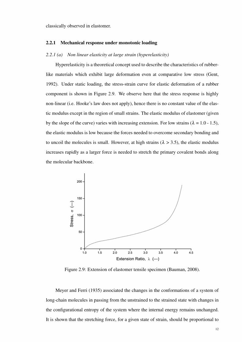
Hyperelasticity is a theoretical concept used to describe the characteristics of rubber-
like materials which exhibit large deformation even at comparative low stress (Gent,
1992). Under static loading, the stress-strain curve for elastic deformation of a rubber
component is shown in Figure 2.9. We observe here that the stress response is highly
non-linear (i.e. Hooke’s law does not apply), hence there is no constant value of the elas-
tic modulus except in the region of small strains. The elastic modulus of elastomer (given
by the slope of the curve) varies with increasing extension. For low strains (λ = 1.0 - 1.5),
the elastic modulus is low because the forces needed to overcome secondary bonding and
to uncoil the molecules is small. However, at high strains (λ > 3.5), the elastic modulus
increases rapidly as a larger force is needed to stretch the primary covalent bonds along
the molecular backbone.
Figure 2.9: Extension of elastomer tensile specimen (Bauman, 2008).
Meyer and Ferri (1935) associated the changes in the conformations of a system of
long-chain molecules in passing from the unstrained to the strained state with changes in
the configurational entropy of the system where the internal energy remains unchanged.
It is shown that the stretching force, for a given state of strain, should be proportional to
12

the absolute temperature, provided that the extension was sufficiently large (see Figure
2.10). Examining this observation with thermodynamic equation:
f =(
∂U∂ l
)T−T
(∂S∂ l
)T. (2.1)
where U is the internal energy, T is the temperature and S is the entropy, it appears that
elasticity of elastomer is essentially entropic in nature.
Figure 2.10: Extension of elastomer tensile specimen (Meyer & Ferri, 1935).
2.2.1 (b) Hyperelastic model
The hyperelasticity of different rubber materials can be described using different
strain energy functions and the majority of these models are incorporated into commercial
FEM software packages. Much work is done to improving the mathematical model with
the following considerations (Mars, 2001):
(a) The model should be able to describe the stress responses to various strain loadings
(uniaxial or biaxial tension/ compression and simple or pure shear) and not be lim-
ited to a single loading condition.
(b) It should involve minimal experimental work to determine the material parameters.
(c) It can be explained physically.
Most of the hyperelastic models have been reviewed. See for the reviews of Treloar
(1975); Laraba-Abbes et al. (2003); Marckmann and Verron (2006). Laraba-Abbes et al.
(2003) classified the hyperelastic models generally into two categories:
13

1. The molecular approach (Gaussian or non-Gaussian network theory) which is based
on statistical thermodynamics considerations.
2. The phenomenological approach: purely continuum approach without directly con-
sidering the microstructure and molecular nature of the material.
Molecular approach (Gaussian network theory) The Gaussian network theory is
based on the concept of a vulcanized rubber being an assembly of long-chain molecules
which are connected with each other at a relatively small number of points to form an
irregular three-dimensional network. The sequence of statistical treatment of the network
is listed below:
1. Calculate the entropy of the whole assembly of chains as a function of the macro-
scopic state of strain in the sample.
2. Derive the free energy or work of deformation.
3. Derive the associated stresses from the work of deformation corresponding to a
given state of strain.
From the first law of thermodynamics, the change in internal energy dU is given by:
dU = δQ+δW. (2.2)
where δQ is the heat absorbed by the system and δW is the work done by the external
forces. In a reversible process, the second law defines the entropy change dS by the
relation:
T dS = δQ. (2.3)
Therefore, for a reversible process, Equation (2.2) becomes
dU = T dS+δW. (2.4)
14

The Helmholtz free energy A, which is the basic to derive the strain energy function,
is defined by the relation:
A =U−T S. (2.5)
For a change of the Helmholtz free energy dA taking place at constant temperature, the
following expression is obtained:
dA = dU−T dS. (2.6)
Inserting Equation (2.4) into Equation (2.6), we have:
dA = δW (constant temperature). (2.7)
which implies that in a reversible isothermal process the change in Helmboltz free energy
is equal to the work done by the applied forces on the system.
Next, consider a unit strained cube which has three equal edge lengths λ1, λ2 and
λ3. For an isochoric deformation, it can be shown that the change in entropy ∆S for the
Gaussian network is given by:
∆S =−12
Nk(λ 21 +λ
22 +λ
23 −3). (2.8)
where N is the number of chains per unit volume (degree of cross linking) while k is the
Boltzmann constant. Taking the basic principles of the kinetic theory and assuming that
there is no change of internal energy during deformation, from Equation (2.6) and (2.7):
W =−T dS. (2.9)
Therefore, Equation (2.8) becomes:
W =12
G(λ 21 +λ
22 +λ
23 −3). (2.10)
where
G = NkT. (2.11)
15

Molecular approach (Non-Gaussian network theory) Under relatively large strains,
the chain response deviates from the Gaussian theory. Therefore, the non-Gaussian net-
work theory which takes into account the finite extensibility of the chain should be consid-
ered. The simplest model of the non-Gaussian network theory is the three-chain model.
This model is based on the assumption that the network of Gaussian chains can be re-
placed by three independent sets of chains parallel to the axes of a rectangular coordinate
system. The four-chain model first developed by Flory and Rehner (1943b) based on
the Gaussian theory is later modified by Treloar (1975) in the non-Gaussian theory. The
model considers an elementary "cell" of the network consisting of four chains radiating
outwards from a common junction point. Following these pioneers, Arruda and Boyce
(1993) proposed a similar chain model but with a distribution of eight chains correspond-
ing to the vertices of a cube inscribed in the unit sphere, namely the eight-chain model.
This model presents better agreement with experimental data for uniaxial and equibiaxial
extensions.
Phenomenological approach The stress-strain behavior of elastomer is often mod-
eled using a pure mathematical approach which is also known as "phenomenological"
approach. The strain energy function or elastic potential W , which corresponds to the
change in the Helmholtz free energy of the material upon deformation, is used to derive
the constitutive equations of elastomeric materials.
A dry elastomer is considered as a continuous body. The natural (undeformed and
unstressed) configuration occupies the region Ω and contains a material point X with
Cartesian coordinates X j ( j = 1,2,3). After deformation, the deformed body occupies the
region Ωd , and the point X is transformed to the spatial position x with coordinates xi (i
= 1,2,3). The deformation gradient tensor, F is given by:
F = Gradx =∂x∂X
. (2.12)
The left Cauchy-Green strain tensor is then simply given by B = FFT . The response
of hyperelastic materials is characterized by the existence of a strain energy function W
16

which depends on F:
W =W (F). (2.13)
Considering the objectivity principle and isotropy, the form of W for incompressible elas-
tomers can be expressed as a function of the two invariants of B, i.e.:
W =W (I1, I2) . (2.14)
where:
I1 = trB I2 =12(I21 − trB2) . (2.15)
Considering the second law of thermodynamics, it can be shown that the Cauchy
stress tensor σ is given by (Holzapfel, 2000):
σ = qI+2[
∂W (I1, I2)
∂ I1+ I1
∂W (I1, I2)
∂ I2
]B−2
∂W (I1, I2)
∂ I2B2 (2.16)
where q is an arbitrary scalar (Lagrange multiplier) due to the incompressibility assump-
tion. It can be determined from the equilibrium equations and appropriate boundary con-
ditions. As indicated in Equation (2.16), the stress response can be entirely determined
once the form of strain energy denstiy W is specified. Table 2.1 summarizes some strain
energy density functions for hyperelastic models (Mars, 2001).
2.2.2 Mechanical response under cyclic loading
When a dry rubber is subjected to cyclic loading, it exhibits strong inelastic responses
such as hysteresis, stress relaxation, Mullins effect and permanent set as shown in Figure
2.11. This figure presents the stress-strain responses of a 50 phr carbon-black filled SBR
subjected to a simple uniaxial tension and to a cyclic uniaxial tension with increasing
maximum stretch every 5 cycles. In the following, the mechanical responses of hysteresis,
stress relaxation, Mullins effect and permanent set are briefly discussed.
17

Table 2.1: Strain energy density functions for hyperelasticity (Mars, 2001).
Constitutive Model Name Strain Energy Density Function
Linear Elastic W = G( v1−2v(ε1 + ε2 + ε3
2)+ ε21 + ε2
2 + ε23 )
Neo-Hookean W = G2 (I1−3)
Mooney-Rivlin W =C10(I1−3)+C01(I2−3)
Generalized Polynomial W = ∑Ni=1 ∑
Nj=1Ci j(I1−3)i(I2−3) j
Ogden W = ∑Nn=1
µnαn(λ αn
1 +λαn2 +λ
αn3 −3)
Gent W =−G2 λmln(1− I1−3
λm)
Arruda-Boyce W = G( 1
2 (I1−3)+ 120λ2m
(I21−9)+ 11
1050λ4m(I3
1−27)
+ 197000λ6
m(I4
1−81)+ 519673750λ8
m(I5
1−243)+···
)Yeoh W =C10(I1−3)+C20(I1−3)2 +C30(I1−3)3
Note: I1 = λ 21 +λ 2
2 +λ 23 , I2 = λ
−21 +λ
−22 +λ
−23
I3 = 1 = λ 21 λ 2
2 λ 23 (Incompressibility constraint)
Figure 2.11: Stress-strain responses of a 50 phr carbon-black filled SBR subjected to a
simple uniaxial tension and to a cyclic uniaxial tension with increasing maximum stretch
every 5 cycles (Diani et al., 2009).
2.2.2 (a) Hysteresis
In Figure 2.12, the unloading curve is well below the uploading curve producing
difference in stress, ∆σ which is called hysteresis. The hysteresis is defined as the amount
18

of energy dissipated during cyclic deformation and characterized by different uploading
and unloading path. It can be related to either viscoelasticity (Bergström & Boyce, 1998),
viscoplasticity (Lion, 1996, 1997) or strain-induced crystallization (Trabelsi et al., 2003)
depending on the material. Hysteresis loss increases with an increase in strain rate, filler
loading, resin loading (at high rates), crosslink density, and strain level but decreases with
an increase in temperature, particle diameter of filler, and resin loading at high testing
temperature (Kar & Bhowmick, 1997).
Figure 2.12: Extension and retraction of tensile specimen exhibiting hysteresis (Bauman,
2008).
2.2.2 (b) Viscoelasticity
Viscoelastic behavior is a time-dependent mechanical response and is usually char-
acterized by creep, stress-relaxation, or dynamic mechanical measurements (Gent, 1992).
Since our study focuses only on stress-relaxation, a detailed review is discussed next.
Stress Relaxation The ability of rubber to retain its elastic behavior after prolonged
compressive stress makes it a favorite material for sealing applications. However, the de-
crease of stress due to viscoelastic behavior in rubber during compression under constant
deformation may reduce the performance of the sealing components after use for a long
period of time (Mostafa et al., 2009). Stress relaxation processes can be categorized into:
a) Physical relaxation where the stress initially decreases rapidly and slows down with
19

time. It is caused by the reorientations of molecular network under constant strain when
secondary bond between chains, fillers and chain and fillers break apart after disengage-
ment and rearrangement of polymer chain. This internal arrangement of polymer network
contributes to the decrease of stress under constant deformation with time. b) Chemical
relaxation which is more prominent in a thin sheet of rubber exposed to chemical and
is associated to scission of chemical bonds in the polymer chains or in the cross-linking
system (Gent, 1992).
2.2.2 (c) Stress-softening (Mullins Effect)
The Mullins effect is the most noticeable effect happening in cyclic deformation. In
Figure 2.13, three cyclic loadings with increasing strain are shown.
Figure 2.13: Mullins effect (Bauman, 2008).
Stress-softening is refers to the decrease of stress level in both the uploading and the
unloading during the first couple of loading cycles. This phenomenon, first observed by
Bouasse and Carrière (1903) then intensively studied by Mullins (1948), is often referred
to as the Mullins effect. While the Mullins effect is well-known in both filled and unfilled
crystallizing dry rubber (Mullins, 1948; Harwood et al., 1966b, 1966a), we have recently
observed the Mullins effect in swollen rubber (Andriyana et al., 2012).
20

2.2.2 (d) Permanent set
When a carbon black filled rubber is loaded to a specific extension and unloaded,
it does not return to its original stress-free configuration but exhibit residual strain or
permanent set as shown in Figure 2.14. Permanent set occurs during unloading when the
old unbroken chain segments try to bring the deformed block back to the original shape,
but are resisted by the new bonds formed by the ruptured chain segments. It increases with
the time in the deformed state and depends on the amount of carbon black in the rubber
and on the maximum elongation of the rubber specimen prior to unloading (Dorfmann
& Ogden, 2004). However, permanent set can be recovered when the recovery time is
sufficient.
Figure 2.14: Permanent set (Bauman, 2008).
2.2.3 Review on the stress-softening in dry rubber
2.2.3 (a) Experimental observations
Diani et al. (2009) reviewed the Mullins effect and concluded several observations
from the materials exhibiting softening effect as listed below:
• Most of the softening, which is characterized by a lower resulting stress for the
same applied strain, appears after the first load.
• After a few cycles (values up to 10 are reported in the literature depending on the
21

material nature), the material responses coincide during the following cycles, aside
from a fatigue effect.
• The softening appears for stretches lower or equal to the maximum stretch ever
applied.
• When the extension exceeds the maximum extension previously applied, the mate-
rial stress-strain response returns to the same path as the monotonous uniaxial ten-
sion test stress-strain response after a transition, which increases with the amount
of strain.
• The softening increases progressively with the increasing maximum stretch.
Filler loading was found to contribute to the stress-softening phenomenon in several
rubber compounds. However, it was also revealed that stress-softening is observed in
unfilled rubber when it is stretched to a stress level similar to the filled rubber (Harwood et
al., 1966b). These unfilled rubbers need to initially contain crystalites like thermoplastic
rubbers or crystallize during the deformation process, such as NBR (Kakavas, 1996).
Although we generally said stress softening occurred in both filled and unfilled rubber,
no stress-softening is observed yet a unfilled non-crystallizing one. It is well documented
by Mullins and Tobin (1957) that non-crystallizing pure gum breaks before any stress
softening is exhibited. Among various observations, we noted here that stress softening
can be recovered by heating or swelling as demonstrated by Harwood and Payne (1966)
and Amin and Lion (2010).
2.2.3 (b) Modeling
As reviewed by Diani et al. (2009), there are many efforts in proposing different
theories to explain the stress-softening phenomenon in dry rubber. Nevertheless, there
is no unanimous microscopic explanation for the stress-softening exists up to this date
(Diani et al., 2009; Marckmann et al., 2002). The first attempt to describe the Mullins
effect is through a phenomenological approach. It was proposed by Mullins and Tobin
(1957) that rubber initially contains both hard and soft phases. During deformation pro-
cess, the hard phase transforms into the soft one. Their theory was successfully adopted
in a number of works (Qi & Boyce, 2004; Beatty & Krishnaswamy, 2000; Huntley et al.,
22

1997, 1996; Wineman & Huntley, 1994). Simo (1987) adopted the concept of Continuum
Damage Mechanics (CDM). The Mullins effect was considered as a damage phenomenon
and was described by a scalar damage parameter. Thus, the material response is charac-
terized by multiplying the classical hyperelastic strain energy with a reducing parameter
representing damage level. Different forms of damage parameter were proposed in the
literature (Chagnon et al., 2004; Ogden & Roxburgh, 1999; Miehe, 1995). In contrast
to Chagnon et al. (2004) and Miehe (1995) who assumed that damage evolves when the
applied level of deformation is undergone by the material for the first time, Ogden and
Roxburgh (1999) proposed that damage stays zero when the material is subjected to a
level of deformation never applied, and evolves in the range of submaximal deformation.
The latter is known as the pseudo-elastic model.
The second approach is through physical interpretation (Marckmann et al., 2002;
Klüppel & Schramm, 2000; Killian et al., 1994; Govindjee & Simo, 1991). Marckmann
et al. (2002) reported the development of a new network alteration theory to describe the
Mullins effect where they considered the Mullins effect as consequence of breakage of
links inside the material, involving both filler-matrix and chain interaction links. This new
alteration theory is implemented by modifying the eight-chains constitutive equation of
Arruda and Boyce (1993). The accuracy of the resulting constitutive equation is demon-
strated on cyclic uniaxial experiments for both natural rubbers and synthetic elastomers.
Chagnon et al. (2006) later modified this network alteration theory to include the dangling
chains effect in the network and proposed that the number of monomers involved in the
elastic response of the material is a decreasing function of the maximum deformation.
2.3 Swelling of elastomers in solvent
The swelling phenomenon of rubber often refers to its solubility in organic media,
e.g. hydrocarbon solvents (Treloar, 1975). Whenever rubbers are exposed to liquids,
one main form of degradation experienced by the materials is swelling which can be
described in terms of mass or volume change (Flory, 1953; Treloar, 1975). During the
swelling, liquids penetrate the polymer network and occupy positions among the polymer
molecules. Consequently, the macromolecules are forced apart resulting in swelling of
material and in a decrease in its strength since the increase in chain separation leads
23

to the reduction of secondary bonding (Callister, 2007). This section discusses physical
description of swelling, thermodynamics of swelling, elastic properties of swollen rubber,
effect of deformation on swelling of the polymers and the coupled theory of the diffusion
and large deformation in polymers.
2.3.1 Physical description
Diffusion of liquid into polymer network involves two physical processes:
1. The liquid molecules first occupy the polymer surface until reaching a concentra-
tion co through adsorption.
2. The liquid penetrates further into the depth of the polymer network until reaching
equilibrium swelling by absorption.
Since the rate of swelling is diffusion-controlled, increasing the square of the elastomeric
components thickness and the viscosity of the liquid will increase the resistance to swelling
of an elastomeric component (Gent, 1992).
2.3.2 Thermodynamics of swelling
Equilibrium swelling in polymer is achieved when the change in free energy result-
ing from the transfer of a small quantity of liquid from the pure liquid phase to the mixed
phase (polymer + liquid) is zero. Treloar (1975) introduced the Gibbs free energy of di-
lution ∆G1 to define the change in the Gibbs free energy of the system due to the transfer
of 1 mol of liquid from the liquid phase to a very large quantity of the mixed phase, given
by:
∆G1 = ∆H1−T ∆S1. (2.17)
where ∆H1 is the heat of dilution which corresponds to the changes in the heat content
H and ∆S1 is the entropy of dilution corresponding to the changes in the entropy S of the
system per mole of liquid transferred from the liquid phase to the mixed phase. The heat
content H is defined by the relation:
H =U + pV. (2.18)
24

where U is the internal energy and V is the volume. When p is the atmospheric pressure,
the second term pV becomes negligible and the H is practically equivalent to U .
At constant pressure, the condition for equilibrium to be achieved with respect to the
transfer of liquid is given by:
∆G1 = 0. (2.19)
To treat swelling problem statistically, it is essential to determine the increase of
mixing entropy of polymer and liquid molecules. The entropy in the mixed state increases
from greater probability compared with the unmixed state, and may be calculated based
on the number of configurations available to the system at any given composition. Flory
(1942) and Huggins (1942) proposed comparatively simple methods for the calculation of
the configurational entropy of mixing. Flory (1942) assumed that the liquid and polymer
molecules are arranged on a three-dimensional lattice of sites such that each site may be
occupied either by a liquid molecule or by a single segment of a polymer chain. Using
this consideration, the entropy of dilution ∆S1 with respect to the liquid component is:
∆S1 =−R ln(1−υ2)+(1−1/x)υ2. (2.20)
where the volume fraction of the fluid in the mixture υ1 is written as 1−υ2 and x is the
segment of the polymer molecules.
For the free energy of dilution ∆G1, Flory introduced the expression for the heat of
dilution ∆H1 on a semi-empirical basis using this formula:
∆H1 = αυ22 . (2.21)
and the Gibbs free energy of dilution ∆G1:
∆G1 = RT(ln(1−υ2)+(1−1/x)υ2 +(α/RT )υ2
2). (2.22)
The alternative solution proposed by Huggins (1942) is similar to the one proposed
by Flory, but includes a more precise analysis of the number of sites available to sub-
25

sequent polymer molecule segments after the third segment. His free energy of dilution
contains an additional term in υ22 but including the same form of heat of dilution as shown
in Equation (2.21), and is expressed as:
∆G1 = RT(ln(1−υ2)+(1−1/x)υ2 +χυ
22). (2.23)
where χ is a parameter which includes a component χo due to additional entropy from
the purely energetic contribution ∆H1, i.e.
χ = χo +α/RT. (2.24)
where χo and α are constants. Note here Equation (2.22) and (2.23) are identical at any
given temperature. In the case where the number of segments in the polymer chain is
sufficiently large, 1/x becomes very small thus these equations reduce to the form
∆G1 = RT(ln(1− v2)+ v2 +χv2
2). (2.25)
where χ is regarded as a constant. This form of equation is often referred to as the Flory-
Huggins equation.
2.3.3 Elastic properties of swollen rubber
Treloar (1975) studied the effect of swelling on the mechanical properties of a cross-
linked rubber by assuming that the unswollen sample is a unit cube which contains N
chains per unit volume. The degree of swelling is defined in terms of the volume fraction
υ2 of the rubber in the mixture of rubber and liquid. Using this definition, and assuming
swelling occurs isotropically, the corresponding linear stretch of the swollen sample is
λo = υ−1/32
The parameter υ2 is introduced to measure the state of swelling of the network,
whether it is in equilibrium or not with respect to the absorption of liquid. The nature of
the swelling agent, or if equilibrium swelling is achieved or not is not considered in the
development of this theory.
Swelling corresponds to isotropic expansion of a network and thus will be accompa-
26

nied by a reduction in the entropy of a network which can be seen from Equation (2.8).
Applying stress on the swollen network will further reduce the entropy due to the defor-
mation of the already swollen network. Therefore the total reduction of entropy involved
during the transformation of the initial unswollen unstrained state to the final strained
swollen can be described by two separate terms. One due to the swelling and one due to
the mechanical loading.
The entropy of deformation ∆S′ of the swollen network (defined per unit volume of
the original unswollen rubber) is given by:
∆S′ = ∆S′o−∆So. (2.26)
where ∆S′o is the total entropy change passing from the unstrained unswollen state to the
strained swollen state. For a Gaussian network (Treloar, 1975), it is given by:
∆S′o =−12
Nk(l21 + l2
2 + l23−3). (2.27)
where l1, l2, and l3 are the lengths of the edges of the original unit cube, i.e. the principal
extension ratios referred to the unswollen state. The change of entropy associated with
the initial isotropic swelling ∆So is given by:
∆So =−12
Nk(3λ2o −3) =−1
2Nk(3υ
− 23
2 −3). (2.28)
Inserting Equations (2.27) and (2.28) into Equation (2.26), we obtain the difference be-
tween these two quantities:
∆S′ =−12
Nk(l21 + l2
2 + l23−3υ
− 23
2 ). (2.29)
The extension ratios of λ1, λ2, and λ3 can be defined with reference to the unstrained
swollen state such that l1 = λ1λ0 = λ1υ− 2
32 , etc. Thus Equation (2.29) becomes:
∆S′ =−12
Nkυ− 2
32 (λ 2
1 +λ22 +λ
23 −3). (2.30)
27

The entropy of deformation ∆S (defined per unit volume of the swollen rubber) is given
by:
∆S = υ2∆S′ =−12
Nkυ132 (λ
21 +λ
22 +λ
23 −3). (2.31)
The corresponding strain energy function for the swollen rubber thus becomes:
W =−T ∆S =12
NkT υ132 (λ
21 +λ
22 +λ
23 −3). (2.32)
Equation (2.32) describes the properties of the swollen rubber in terms of the exten-
sion ratios measured in the swollen state and the volume fraction of rubber υ2. Noted
here N is the number of chains per unit volume of the unswollen rubber. Comparing the
results of swollen rubber expressed in Equation (2.32) with the corresponding expression
of the unswollen rubber in Equation (2.10), it is seen that the dependence of the stored
energy on strain are the same in both cases, except the value of the shear modulus. Thus,
we can write:
G′ = Gυ132 = ρRT/Mcυ
132 . (2.33)
where G is the modulus in the unswollen state while G′ is the modulus in the swollen
state and ρ is the density in the unswollen state. This result implies that the only effect
of swelling is to reduce the modulus in inverse proportion to the cube root of the swelling
ratio, without changing the form of the stress-strain relations. Moreover, as stated by
Treloar (1975) that from a physical standpoint, swelling is a purely physical mixing or
interdiffusion process in which there is no chemical attraction between the rubber and
liquid molecules.
2.3.4 Effect of deformation on swelling
The effect of deformation in terms of applied strain or stress on the swelling of a
polymer network has long been recognized and discussed by Flory and Rehner (1943a).
The theory was further developed by Treloar (1975, 1950) and he discussed it for general
types of homogeneous strain. Equations for uniaxial extension, bi-axial extension and
uniaxial compression strains were developed. He concluded from the experimental data
obtained from vulcanized natural rubber specimens swollen in benzene and heptane that
28

the effect of strain on the equilibrium swelling is satisfactorily predicted for the statistical
theory under the three entirely different types of strains. Although swelling under uni-
directional compression is the least accurate due to the measuring process that required
drying and weighing and lengthy immersion duration, however it is observed that swelling
is increasing under tensile strain and decreasing with compressive strain.
Horkay and Zrinyi (1988) compared the effect of deformation and diluent activity
on the equilibrium concentration of poly(vinyl acetate) networks swollen with toluene.
The swollen gels were deswollen by two methods: gels were subjected to uniaxial com-
pression at fixed activity of the diluent and the activity of the diluent around the free
swollen gel specimens was lowered by dissolving a polymer in the surrounding media.
They compared the experimental volume fraction data obtained from uniaxial deformed
gels equilibrium swollen in pure diluent with calculated values using Equation (2.34).
φ = φeΛ−4/9e (2.34)
where φ is the volume fraction of deswollen gels, φe is the volume fraction of the poly-
mer in the freely swollen gel and Λe is the deformation ratio relative to the length of the
freely swollen undeformed gel. It is found that there is a good agreement between mea-
sured and calculated volume fraction data in the cases of natural rubber samples swollen
by benzene and heptane conducted by Treloar (1950) and poly(vinyl acetate) networks
swollen by toluene in their study. They evaluated the relationships between the swelling
pressure, elastic modulus, deformation ratio and polymer concentration and validated this
relationship with experimental results.
Fukumori et al. (1990) utilized real time pulse Nuclear Magnetic Resonance (NMR)
to evaluate the initial swelling rate of the filled and unfilled NBR under tensile deforma-
tion swollen in non polar solvent, e.g. Carbon Tetrachloride (CCl4) as shown in Figure
2.15. The specimen studied is a ring specimen with outside diameter = 22mm and in-
ner diameter=19mm. The rubber contents filler concentration of 0, 20, 40 and 60 phr.
The swelling ratio of the rubber matrix at equilibrium is evaluated with volume swelling
measurements. They found that the initial swelling rate and the swelling ratio of the rub-
ber matrix at equilibrium increased with the increase of the stretch ratio. The molecular
29

mobility of the swollen rubber is also enhanced with the increase of the tensile strain.
It was found that the presence of reinforcing filler in NBR reduced the initial swelling
rate because of transient spatial effect caused by some oriented structures induced by
tensile deformation. However, the presence of reinforcing fillers in the swollen rubbers
under tensile strain has a strain amplification effect proportionally to the filler concen-
tration, which resulted in an increase of the average local strain in the rubber matrix and
enhanced the swelling ratio relative to the unfilled system.
Figure 2.15: Schematic illustration of the real-time NMR, measurement of a stretched
rubber specimen immersed in a solvent (Fukumori et al., 1990).
A free oscillation technique has been adopted to study the effect of swelling on
the dynamic storage and loss moduli of carbon black filled and unfilled natural rubber
materials on a range of tensile pre-strains (Busfield et al., 2000). It is observed that the
dynamic storage and loss moduli are independent of the pre-strain at small pre-strains.
Both the storage and the loss moduli increase with pre-strains. Swelling the materials
in liquids with a wide range of viscosity produces a relatively large decreases in both
the storage and the loss moduli. The authors attributed the dynamic behaviour of the
swollen filled rubbers to the combined effects of a reduction in the modulus of the rubber
matrix (caused by the swelling action) and a reduction in the effective volume fraction
of the filler. However, the effect of the viscosity of the swelling liquid on these dynamic
30

behaviours are insignificant. They concluded that the swelling liquids might be affecting
the filler-filler or the filler-rubber interaction.
Botros and Sayed (2001) investigated the effect of compressive strain on the swelling
behavior of different blend compositions of NR/Ethylene Propylene Diene Monomer
(EPDM) swollen in motor oil. The compression recovery of all blend ratios investigated
had positive values at low applied compression strain (3%). However, at high compressive
strain (18% and 35%), the compression recovery had negative values. The lowest weight
uptake of motor oil was shown by the EPDM vulcanizate, whereas the 25/75 NR/EPDM
blend showed the highest compression recovery.
Most recently, Nah et al. (2011) investigated the swelling of bent natural rubber
sheet in dodecane. Following Treloar’s theory, they proposed that when rubber sheets are
bent, they are expected to swell more on the tension side and less on the compression
side. Moreover, when the bending constraint is removed, recovery toward the initial flat
state is expected to be only partial at first and then followed by a slow further recovery.
They found that the measured "set" following release from bending is agreed with simple
swelling theory. The time dependence of later recovery is shown to be in agreement
with the rate of diffusion of the swelling liquid. It is concluded that internal migration
of compatible liquids will cause temporary delays in deformation kinetics and make a
significant contribution to energy losses. Also, the bending experiment itself appears to
provide a simple and generally applicable method for determining the internal diffusion
coefficients of absorbed liquids.
2.3.5 Modeling of coupling between deformation and swelling
Several theories have been developed to account for the coupled diffusion and large
deformation in polymers (Gandhi, 1989; Inci et al., 2001; Baek & Srinivasa, 2004; Ram-
tani, 2006; Hong et al., 2008; Deng & Pence, 2009; Soares, 2009; Hong et al., 2009;
Deng & Pence, 2010; Joshi & Muliana, 2010; Cai et al., 2010; Nah et al., 2011; Johlitz
& Lion, 2012). Gandhi (1989) considered the problem of a cylindrical specimen of a
nonlinearly elastic solid and an ideal fluid medium subjected to combined finite axial ex-
tension and torsion. He discussed the general problem for the finite deformation of the
swollen cylinder in the context of Mixture Theory and presented the computational results
31

for the variation of the radial and tangential stretch ratios and the distribution of the fluid
in the swollen deformed state. He found that the swollen volume of a cylinder reduces
with twisting when the axial extension ratio is held constant. Simulation agreed well with
experimental results.
Baek and Srinivasa (2004) modeled slow diffusion of a fluid into a swelling solid
undergoing large deformation and predicted the stress in the solid as well as the diffu-
sion rates. The approach is based on the balance laws of a single continuum with mass
diffusion, and overcame the difficulties inherent in the theory of mixtures in specifying
boundary conditions. The authors derived a "natural" boundary condition based on the
continuity of the chemical potential by the use of a variational approach, based on max-
imizing the rate of dissipation. They found that the differential equations resulting from
the use of mixture theory can be recast into a form that is identical to the equations ob-
tained in the absence of the initial effect and they successfully solved the boundary value
problem of the steady flow of a solvent through a gum rubber membrane.
Hong et al. (2008) formulated a theory of the coupled mass transport and large de-
formation. The free energy of the gel results from two molecular processes: stretching
the network and mixing the network with the small molecules. They assumed that both
the small molecules and the long polymers are incompressible, a constraint enforced by
using a Lagrange multiplier, which coincides with the osmosis pressure or the swelling
stress. The gel can undergo large deformation of two modes. The first mode results from
the fast process of local rearrangement of molecules, allowing the gel to change shape
but not volume. The second mode results from the slow process of long-range migration
of the small molecules, allowing the gel to change both shape and volume. They also as-
sumed that the local rearrangement is instantaneous, and model the long-range migration
by assuming that the small molecules diffuse inside the gel. The theory is illustrated with
a layer of a gel constrained in its plane and subject to a weight in the normal direction.
Soares (2009) described a single-constituent constitutive model for diffusion of flu-
ids in nonlinear elastic solids, originally presented by Baek and Srinivasa (2004) and
based on a variational method and on the assumption of continuity of chemical poten-
tial across the solid-fluid interface. The balance laws for a single continuum with mass
diffusion are cast in spherical coordinates, and suitable boundary conditions are posed to
32

describe the radial diffusion of fluid through an elastic spherical shell with finite thickness.
They modeled its inner surface adjacent to a rigid wall, either impermeable or permeable,
while the outside surface is in contact with the fluid that swells the solid, diffuses through
it, and exerts a hydrostatic pressure on its surface.
Hong et al. (2009) investigated the effect of mechanical load and geometric con-
straint on the inhomogeneous swelling of a polymeric gel. When the network, solvent,
and mechanical load equilibrate, inside the gel the chemical potential of the solvent is
homogeneous, but the concentration of the solvent and the deformation of the network
can be inhomogeneous. They used the chemical potential of the solvent and the deforma-
tion gradient of the network as the independent variables of the free-energy function, and
concluded that the boundary value problem of the swollen gel is equivalent to that of a hy-
perelastic solid. They implemented the approach in a finite-element package, ABAQUS,
and analyzed examples of swelling-induced deformation, contact, and bifurcation.
Deng and Pence (2009) considered the connection between diffusion and large de-
formation in polymer and the broader hyperelastic theory that treats the effect of mechan-
ical loading in deforming the swollen polymer network. They pointed out that fluid loss
(swelling reduction) or fluid gain (swelling increase) occurred when there is a change in
mechanical loading. In such cases the gel reestablishes equilibrium only when the rela-
tive motion of the liquid through the polymer has ceased and processes have come to rest.
Such processes are inherently dissipative. Their study focused on reestablished equilib-
ria depending on mechanical load. They considered that the amount of available fluid is
limited for quasi-static loadings that give fluid gain. It is predicted that maximum fluid
gain in the gel system will be reached by increasing the quasi-static loading. The gel sys-
tem transitions from a saturated state to an unsaturated state. This quasi-static transition is
considered in the context of homogeneous deformation where an appropriate hyperelastic
analysis shows that the equilibrium mechanical response is inherently stiffer after loss of
saturation. They concluded from the study of inhomogeneous deformation of an everted
tube subject to an axial load and found that loss of saturation leads to an inherently stiffer
quasi-static response.
In addition, Deng and Pence (2010) discussed a continuum model for the absorp-
tion and redistribution of fluid in swollen elastomers due to mechanical loading for both
33

saturated and unsaturated systems. They considered the effect of various boundary dis-
placement and traction in the problem of radial displacement combined with azimuthal
shear for an annular cylinder consisting of a fluid infused hyperelastic medium. The fluid
distribution is monitored through a numerical model. It is found that certain boundary
tractions generate overall volume increase after free swelling and the overall mechanical
response after loss of saturation is stiffer than the saturated system.
Cai et al. (2010) suggested that when an elastomer imbibes a solvent and swells, a
force is generated if the elastomer is constrained by a hard material. The magnitude of
the force depends on the geometry of the constraint, as well as on the chemistry of the
elastomer and solvent. They modeled an elastomer crosslinked on the exterior surface of
a metallic tubing. The elastomer then imbibes a solvent and swells. After the swollen
elastomer touches the wall of the borehole, a significant amount of time is needed for
the solvent in the elastomer to redistribute, building up the sealing pressure to the state of
equilibrium. They calculated the sealing pressure and the sealing time from the geometric
parameters (i.e., the thickness of the elastomer and the radii of the tubing and borehole),
the number of monomers along each polymer chain of the elastomer, and the affinity
between the elastomer and the solvent.
2.4 Biodiesel
2.4.1 What is biodiesel?
Biodiesel fuels are methyl ester based oxygenates derived from a wide range of re-
newable natural sources such as animal fats (beef tallow), vegetable oils (soybean oil,
cottonseed oil, canola oil), and recycled cooking grease or oils (e.g., yellow grease)
(Trakarnpruk & Porntangjitlikit, 2008). It is a diesel replacement fuel in a compression
ignition (CI) engine.
The biodiesel is manufactured through transesterification which can be illustrated in
Figure 2.16. The transesterification process converts oils and fats into chemicals called
long-chain mono alkyl esters, or biodiesel. These chemicals are better known as fatty
acid methyl esters (FAME) (Laboratory, 2009). From the schematic diagram, it is easy to
explain that the oil/fat are reacted with a short-chain alcohol (i.e. methanol) with the aid
of a catalyst (i.e. sodium hydroxide (NaOH) or potassium hydroxide (KOH)) to produce
34

biodiesel and glycerin. Glycerin is a sugar alcohol that is formed as by-product in the
manufacturing process of biodiesel.
Figure 2.16: Basic transesterification process (Laboratory, 2009).
Biodiesel has been proven to be environmentally friendly and to provide properties
similar to that of conventional fuel. However, the biodiesel has a different composition
than conventional diesel. Indeed, while biodiesel consists of a mixture of fatty acid es-
ter, conventional fuel consists of a mixture of hydrocarbon (Haseeb et al., 2010). This
change of composition leads to difficulties in terms of material compatibility especially
in industrial applications involving elastomeric materials.
2.4.2 Effect of biodiesel on elastomers
Compatibility studies of several types of elastomers in diesel and palm biodiesel
have been conducted (Trakarnpruk & Porntangjitlikit, 2008; Haseeb et al., 2010, 2011).
However in these works, only physical degradation related to the swelling, hardness and
tensile strength of materials was studied.
The material compatibility has been studied by Trakarnpruk and Porntangjitlikit
(2008) who evaluated six types of elastomer (NBR, Hydrogenated Nitrile Butadiene Rub-
ber (HNBR), NBR/ Polyvinyl Chloride (PVC), acrylic rubber, co-polymer Fluorocarbon
rubbers (FKM), and terpolymer FKM) in B10 (10% palm biodiesel in diesel) after im-
mersion of 22, 670, and 1008 h at 100C. They found that NBR, NBR/PVC and acrylic
rubber were affected more than other elastomers due to the absorption and dissolving of
35

biodiesel by rubber in these samples and concluded that Co-polymer FKM and terpolymer
FKM are more resistant in B10 biodiesel environment.
Haseeb et al. (2010) evaluated the degradation behaviour of NBR, CR, and fluoro-
viton A in B0 (diesel), B10, B100 (palm biodiesel) after 500 h immersion at (25C)
room temperature and 50C. The mass and volume change, hardness, tensile strength
and elongation were investigated. The exposed elastomer surface was studied by Scan-
ning Electron Microscope (SEM). Fourier Transform Infrared (FTIR) spectroscopy was
conducted to identify the chemical and structural changes. It is found that the physical
degradation was higher for both CR and NBR while fluoro-viton has good resistance in
biodiesel.
In addition, Haseeb et al. (2011) investigated the physical property degradation of
EPDM, Silicone Rubber (SR), Polytetrafluroethylene (PTFE) CR, and NBR upon ex-
posure to diesel and palm biodiesel. Static immersion tests in B0 (diesel), B10 (10%
biodiesel in diesel), B20, B50 and B100 (biodiesel) were carried out at (25C) room tem-
perature for 1000 h. They measured changes in weight and volume, hardness and tensile
strength at every 250 h of immersion time. Compositional changes in biodiesel due to
exposure of different elastomers were investigated by Gas Chromatography Mass Spec-
troscopy (GCMS). They concluded that the overall sequence of compatible elastomers in
palm biodiesel is found to be PTFE > SR > NBR > EPDM > CR.
Other than palm biodiesel, compatibility studies of rubber components in other types
of biodiesel are investigated (Maru et al., 2009; Berlanga-Labari et al., 2011). Maru et
al. (2009) analyzed the interaction between three fuels (petroleum diesel and two types
of biofuel: soybean and sunflower) and High Density Polyethylene (HDPE) after static
immersion of 75 and 125 days under constant temperature of 60C. A wide range of
characterization methods were used to evaluate the changes in both rubber materials and
the fuels: including weight change measurement, optical, scanning electron and Atomic
Force Microscopies (AFM), Raman and FTIR and differential scanning calorimetry. They
detected the maximum weight gain by fluid absorption in the polyethylene immersed in
petroleum diesel by the spectroscopic techniques. However, no significant differences in
the HDPE surface morphology after immersion in these fuel medias. They concluded that
ageing took place only in biodiesels, but this phenomenon did not cause degradation or
36

corrosion of HDPE, since petroleum diesel did not age but exerted the most significant
material degradation.
On the other hand, Berlanga-Labari et al. (2011) also evaluated the compatibility of
the same material (HDPE) but in E5 (5% v/v bioethanol, 95% v/v gasoline) and E10 (10%
v/v bioethanol, 90% v/v gasoline) after static immersion of 2000 h at 45C. Different
mechanical and physical-chemical properties of HDPE have been assessed before and
after the execution of these tests. Additional information about biofuels-HDPE interaction
has been obtained by infrared spectroscopy and solubility tests. Although they observed a
slight variation of mechanical properties in HDPE, both studies concluded that no defects
on the chemical structure and physical properties of this polymer have been detected.
Moreover, there are collections of experimental studies on mechanical responses of
polymeric gels in solvents (Sasaki, 2004; Hirotsu, 2004; Valentín et al., 2010). Neverthe-
less, it is to note that the works focusing on the effect of palm biodiesel diffusion on the
macroscopic mechanical responses of the rubber components, in particular under cyclic
and fatigue loading conditions, are less common.
37

CHAPTER 3
RESEARCH METHODOLOGY
The literature review has shown that very limited work has been done on studying the
mechanical responses, i.e. hysteresis, stress-softening, etc. of swollen rubber under cyclic
loading conditions. The present research is therefore carried out to establish a database
of swollen rubbers, namely NBR and CR using mechanical tests. The mechanical tests
involved are compressive cyclic test and compressive multiple relaxation test.
Experimental procedures to prepare swollen rubbers, including the design of the
uniaxial compression test specimen, the development of an original compression device
and details of the immersion test are described in this chapter. The swelling behaviours for
both stress-free and uniaxially-stressed rubber specimens are investigated. Subsequently,
the following mechanical responses are investigated: stress-softening and hysteresis from
compressive cyclic test and viscoelasticity from compressive multiple relaxation test.
Next, the stress-softening in swollen rubbers is modeled using an extended pseudo-
elastic model and an extended two-phase model. These are conducted as a first attempt
towards understanding and modeling of the stress-softening phenomenon in swollen rub-
bers.
The overall research work is described using flow chart in Figure 3.1.
Remark 1 It is to note that large parts of the content in this chapter and the following
chapters have been published (Chai et al., 2011; Andriyana et al., 2012; Chai, Andriyana,
et al., 2013; Chai, Verron, et al., 2013). The rest of the thesis is written based on the inspi-
ration from these papers, aiming at producing a well-organized and easy to understand
research output.
38

Figure 3.1: General research methodology.
39

3.1 Experimental program
3.1.1 Materials and specimen geometry
Commercial grade NBR and CR with 60 shore hardness are purchased from MAKA
Engineering Sdn. Bhd., Malaysia. The NBR and CR have a specific gravity of 1.4 ± 0.1
and 25 wt.% of carbon black. Due to confidentiality constraints, the detailed compound
ingredients are not provided here. For each type of rubber compound, the vulcanization
process is performed by compression molding process at 165 °C for 5 min under a pres-
sure of approximately 6.89 MPa from an electrical resistance heating press. The rubber
specimens for swelling and mechanical tests are annular cylindrical blocks. Note that no
standard is followed in the determination of specimen geometry. The wall thickness of
the specimen is optimized with the help of finite element simulation software to ensure
that equilibrium diffusion (swelling) in the rubber can be achieved within a reasonable
period of time and the wall thickness is able to sustain the compression load to prevent
buckling. It is found that the optimum height, outer diameter and wall thickness of the
specimen are respectively 10 mm, 50 mm and 6 mm.
Different biodiesel blends are prepared by blending palm biodiesel (provided by Am
Biofuels Sdn. Bhd., Malaysia) with diesel. Table 3.1 shows the analysis report of the
investigated palm biodiesel. The palm biodiesel blends prepared are B0 (100% diesel),
B25 (blend of 25% of biodiesel and 75% of diesel), B75 (blend of 75% of biodiesel and
25% of diesel) and B100 (100% biodiesel).
3.1.2 Experimental setup
3.1.2 (a) Swelling tests on stress-free specimens (free swelling)
The tests are conducted in diesel (B0) and biodiesel (B100) respectively at room
temperature for various immersion durations: 2, 5, 10, 20 and 30 days. Figure 3.2 shows
the simple immersion test where the specimens are hung and immersed in a stainless steel
container containing biodiesel. Each specimen is completely immersed in the tested fuel.
Thereby allowing stress-free swelling to occur in the rubber specimens.
40

Table 3.1: Properties of B100 palm biodiesel.
Test Unit Methods Results
Ester content % (m/m) EN 14103 96.9
Density at 15C kg/m3 EN ISO 12185 875.9
Viscosity at 40C mm2/s EN ISO 3104 4.667Flash point C EN ISO 3679 168Cetane number - EN ISO 5165 69.7Water content mg/kg EN ISO 12937 155Acid value mgKOH/g EN ISO 3679 0.38Methanol content % (m/m) EN 14110 <0.01Monoglyceride content % (m/m) EN 14105 0.67Diglyceride content % (m/m) EN 14105 0.2Triglyceride content % (m/m) EN 14105 0.2Total glycerine % (m/m) EN 14105 0.25
Figure 3.2: Swelling test on stress-free specimens. Before (left) and after (right) immer-
sion in tested fuel (B100).
3.1.2 (b) Swelling tests on uniaxially-stressed specimens (constrained swelling)
The specially made rubber specimens are compressed to different degrees of com-
pressive strain by attaching them to a custom-made compression device prior to immer-
sion as shown in Figure 3.3. The compression device has special features as described
below:
41

Figure 3.3: Compression device.
1. It consists of four rectangular stainless steel plates. Stainless steel plates are used
for corrosion resistance because the device is needed to be immersed into diesel
and biodiesel which are deemed to be corrosive.
2. The device is able to accommodate a total of 12 specimens arranged in 3 different
levels between two successive plates.
3. Each plate has 4 main holes to allow the liquid to flow and diffuse into the inner
surface of the rubber specimens. In this way, each rubber specimen is subjected
to diffusion of liquid from both inner and outer wall surfaces, i.e. diffusion along
radial direction only as illustrated in Figure 3.4.
42
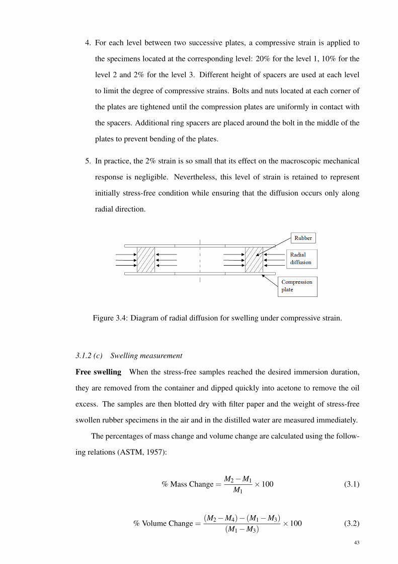
4. For each level between two successive plates, a compressive strain is applied to
the specimens located at the corresponding level: 20% for the level 1, 10% for the
level 2 and 2% for the level 3. Different height of spacers are used at each level
to limit the degree of compressive strains. Bolts and nuts located at each corner of
the plates are tightened until the compression plates are uniformly in contact with
the spacers. Additional ring spacers are placed around the bolt in the middle of the
plates to prevent bending of the plates.
5. In practice, the 2% strain is so small that its effect on the macroscopic mechanical
response is negligible. Nevertheless, this level of strain is retained to represent
initially stress-free condition while ensuring that the diffusion occurs only along
radial direction.
Figure 3.4: Diagram of radial diffusion for swelling under compressive strain.
3.1.2 (c) Swelling measurement
Free swelling When the stress-free samples reached the desired immersion duration,
they are removed from the container and dipped quickly into acetone to remove the oil
excess. The samples are then blotted dry with filter paper and the weight of stress-free
swollen rubber specimens in the air and in the distilled water are measured immediately.
The percentages of mass change and volume change are calculated using the follow-
ing relations (ASTM, 1957):
% Mass Change =M2−M1
M1×100 (3.1)
% Volume Change =(M2−M4)− (M1−M3)
(M1−M3)×100 (3.2)
43

where M1 and M2 are the mass in air (gram) before and after immersion while M3 and
M4 are mass in water (gram) before and after immersion. For each test, at least four
specimens are used to measure volume and mass changes.
Constrained swelling The test procedure for swelling measurement of uniaxially-stress
free swollen specimens is summarized as followed:
1. Before the immersion, the weight of the rubber specimen is measured in air and in
distilled water. The specimen is then quickly dipped into alcohol and blotted dry
with filter paper.
2. After weight measurement, the rubber specimens are placed in sequence on the
compression plates. Grease is applied on the surface of the specimens that are in
contact with the compression plate to avoid bulging and hence ensuring that the
specimens are in a simple uniaxial compressive stress state.
3. Bolts and nuts are used to tighten the compression device until the compression
plates are uniformly in contact with the spacers. The device containing rubber
specimens is subsequently immersed into different palm biodiesel blends for dif-
ferent durations. The detail of the immersion tests is given in Table 3.2. All the
tests are conducted at room temperature.
4. At the end of each immersion period, the specimens are removed from the compres-
sion device and quickly dipped into acetone; they are then cleaned with filter paper
to remove the excess oil. Specimens are left for 30 minutes to allow for recovery
before any measurement is made after immersion.
5. Step 1 is repeated to measure the weight of rubber specimen after immersion.
The percentages of mass change and volume change are calculated following Equa-
tions (3.1) and (3.2)
44

Table 3.2: Immersion tests.
Biodiesel Blend Level of Compressive Strain (%) Immersion Duration (days)
B0 2/10/20 30/90
B25 2/10/20 30/90
B75 2/10/20 30/90
B100 2/10/20 30/90
3.1.2 (d) Mechanical tests
To gain insight in the effect of swelling due to solvent diffusion, on the mechanical
response of swollen rubber, mechanical tests on dry and swollen samples are carried out
using an Instron 5500 uniaxial test machine equipped with a 10 kN load cell at room
temperature. Circular compression plates are attached to the machine to ensure uniform
displacement control on the specimens. The experimental setup is connected to a com-
puter to record the experimental data. The tests are conducted at a constant displacement
rate of 0.1 mm/s to avoid excessive increase in the temperature of the specimens, i.e. tem-
perature effects are not considered in the present study. Figure 3.5 shows the experimental
setup of the compression test.
Figure 3.5: Experimental setup of the compression test.
45

Two types of mechanical tests are conducted:
1. Cyclic compression test: This is conducted to observe the stress-softening and hys-
teresis behaviors of the rubber. The test is conducted at 0.01 s−1 strain rate using
displacement-controlled mode with two different maximum compressive strains,
30% and 40%, of 6 cycles each.
2. Multi-relaxation test: This test is conducted to observe the viscoelasticity of the
rubber. The test is conducted at 0.01 s−1 strain rate using displacement-controlled
mode initially with 6 cycles of maximum compressive strain of 40% to remove the
stress-softening effect. It is then followed by compressing the specimen to strain
levels of 10%, 20% and 30% and hold it for 30 minutes as illustrated in Figure 3.6.
The stress during the holding time is recorded for both loading and unloading of
the strain levels.
In order to ensure repeatability of the results, at least three specimens are used in
each test.
Figure 3.6: Multi-relaxation test.
3.1.2 (e) Microstructure observations
The dry and swollen specimens were cut with a sharp blade and the cross sectional
surface was observed with a low vacuum and low pressure scanning electron micro-
scope (FE1 Quanta FEG 250). The aim is to obtain information regarding microstructural
change due to oil penetration.
46

3.2 Continuum mechanical modeling
As a first step to modeling the mechanical response of swollen rubber under cyclic
loading, only the Mullins effect is considered. Other inelastic phenomena such as per-
manent set, hysteresis, etc. will not be considered. For this purpose, data treatment is
required and will be discussed in Section 5.1 in Chapter 5.
The constitutive equations of swollen rubber experiencing irreversible softening (dam-
age) due to cyclic mechanical loading is addressed. For this purpose, we first layout the
chemical potential equation to obtain the Flory-Huggins interaction parameter for differ-
ent rubber-fuel combinations. These parameters are needed for continuum mechanical
modeling of the Mullins effect in swollen rubber. Next, the discussion is confined to the
hyperelasticity of swollen rubber with and without internal damage. The classical multi-
plicative decomposition of the deformation gradient tensor into swelling and mechanical
parts is adopted to replicate the experimental procedure whereby the rubber is first sub-
jected to isotropic swelling before undergoing mechanical loading. The stress response is
then derived by considering the second law of thermodynamics.
In order to capture the Mullins effect in swollen rubber, two models available in the
literature are considered: the pseudo-elastic model of Ogden and Roxburgh (1999) and
the two-phase model of Mullins and Tobin (1957) and Qi and Boyce (2004). These two
models are extended to account for the effect of swelling.
3.2.1 Determination of the Flory-Huggins interaction parameter, χ
The Flory-Huggins Interaction parameter χ , is the dimensionless interaction param-
eter describing the interaction between rubber and solvent, i.e. palm biodiesel and diesel.
Following the Flory-Huggins equation from Equation (2.25), these parameters can be
calculated at equilibrium swelling using the following chemical potential equation:
kTνC0
[ln(
1− 1Je
s
)+
1Je
s+χ
1(Je
s )2
]+(Je
s )−1/3− (Je
s )−1 = 0 (3.3)
where k is Boltzmann constant, T is temperature during swelling, ν is the molar volume
of the solvent molecules, Co is the dry shear modulus and Jes is equilibrium degree of
swelling.
47

3.2.2 Hyperelasticity of swollen rubber
3.2.2 (a) Description of the deformation
In the experimental procedure, stress-free dry rubber specimens are immersed in a
solvent to allow isotropic swelling to occur in the material. After a desired degree of
swelling is achieved, the resulting swollen specimens are subjected to various mechanical
loadings. The corresponding procedure is illustrated in Figure 3.7.
V0 Vs V =Vs- -Fs Fm
(C0) (Cs)(Ct)
6F = FmFs
Figure 3.7: Illustration of experimental procedure.
Initially, the rubber specimen is in a dry state at C0 (unswollen-unstrained configura-
tion) having a volume of V0. It undergoes isotropic swelling characterized by the swelling
part of the total deformation gradient F, denoted Fs. Due to swelling, the specimen vol-
ume changes to Vs at Cs (swollen-unstrained configuration). The degree of swelling, Js, is
simply defined by the ratio between the volume of swollen specimen Vs and the volume
of dry specimen V0, i.e.
Js =Vs
V0. (3.4)
Consequently, Fs can be written as a function of Js as follow:
Fs = J1/3s I (3.5)
where I is the identity tensor.
The next stage of deformation consists of imposing a mechanical loading on the
swollen specimen. The corresponding deformation is characterized by the mechanical
part of the deformation gradient tensor, denoted Fm. Here, it is assumed that the swollen
48

rubber undergoes deformation at constant volume, i.e. swollen rubber is assumed to be
incompressible. Thus, the kinematic constraint to respect during this stage of deformation
is det Fm=1. In summary, the transformation of material from C0 to Ct (swollen-strained
configuration) can be described by:
F = FmFs = J1/3s Fm. (3.6)
Noted that the above decomposition is originally proposed by Flory (1961). Thermal
expansion effects can be taking into accouny in a similar way.
3.2.2 (b) Constitutive equations
General stress response In order to describe the stress response, we postulate the exis-
tence of a strain energy function W , defined per unit of volume in C0, which depends on
the degree of swelling Js and on the mechanical part of deformation gradient tensor Fm
as follows:
W = W (F) = W (Js,Fm) =Ws(Js)+ JsWm(Js,Fm). (3.7)
In this expression, Ws is the strain energy per unit of volume in C0 associated with
isotropic swelling while Wm is the strain energy associated with mechanical loading. It is
to note that Wm is defined per unit of volume in Cs. Moreover, the dependence of Wm on
Js is through material parameters which explicitly depend on the degree of swelling.
For a purely mechanical process, the second law of thermodynamics reduces to:
D = P : F−W ≥ 0 (3.8)
where D is the internal dissipation per unit of volume in C0, P is the 1st Piola-Kirchhoff
stress tensor relative to C0 (engineering stress with respect to unswollen-unstrained con-
figuration). For swollen rubber of a given degree of swelling (constant degree of swelling),
the rate of change of the strain energy W is given by:
W =∂W∂Js
∣∣∣Fm
Js +∂W∂Fm
∣∣∣Js
: Fm
=∂W∂Fm
∣∣∣Js
: Fm (3.9)
49

since Js = 0.
In view of Equation (3.6), Fm can be related to F through:
F =˙
J1/3s Fm =
13
J−2/3s JsFm + J1/3
s Fm. (3.10)
Thus, the internal dissipation becomes:
D =
(J1/3
s P− ∂W∂Fm
∣∣∣Js
): Fm = 0. (3.11)
which must be satisfied for all possible values of Fm respecting the incompressible con-
straint, i.e. (Holzapfel, 2000):
detFm = 1 ⇔ ˙detFm = 0 ⇔ F-Tm : Fm = 0. (3.12)
Considering Equation (3.11) and the right term of Equation (3.12), we deduce:
(J1/3
s P− ∂W∂Fm
∣∣∣Js
)= qF-T
m . (3.13)
where q is an arbitrary scalar (Lagrange multiplier) due to incompressibility assumption
which can be determined from the equilibrium equations and appropriate boundary con-
ditions. Hence, we obtain the stress response as follow:
P = qJ−1/3s F-T
m + J−1/3s
∂W∂Fm
∣∣∣Js. (3.14)
Recalling Equation (3.7), the above equation can be recast to:
P = qJ−1/3s F-T
m + J2/3s
∂Wm
∂Fm. (3.15)
The Cauchy stress tensor σ (defined in Ct) is simply given by:
σ = (detF)−1PFT = J−1s
(qJ−1/3
s F-Tm + J2/3
s∂Wm
∂Fm
)FT
= qJ−1s I+
∂Wm
∂FmFT
m.
50

Noting that (Holzapfel, 2000):
∂Wm
∂FmFT
m = Fm
(∂Wm
∂Fm
)T
= 2Fm∂Wm
∂CmFT
m. (3.16)
where Cm = FTmFm, the Cauchy stress tensor becomes:
σ = qJ−1s I+2Fm
∂Wm
∂CmFT
m. (3.17)
Assuming that swollen rubber is isotropic, we may express Wm(Js,Cm)=Wm(Js, I1m, I2m),
where:
I1m = trCm I2m =12(I1m− trC2
m). (3.18)
Using chain rules, the above expression can be recast to:
σ = qJ−1s I+2
[(∂Wm
∂ I1m+ I1m
∂Wm
∂ I2m
)Bm−
∂Wm
∂ I2mB2
m
]. (3.19)
where Bm = FmFTm. The 1st Piola-Kirchhoff stress tensor relative to Cs (engineering
stress with respect to swollen-unstrained configuration), P, can be obtained from P =
(detFm)σF-Tm , which yields:
P = qJ−1s F-T
m +2[(
∂Wm
∂ I1m+ I1m
∂Wm
∂ I2m
)Fm−
∂Wm
∂ I2mFmCm
]. (3.20)
Finally, recalling that σ = (detF)−1PFT, the tensors P and P are simply related through:
P = J2/3s P. (3.21)
Special case of uniaxial extension Without loss of generality, we focus on the special
case when the swollen rubber is subjected to uniaxial extension along the e1 direction. In
this case, the tensors Fm and Bm are simply given by:
Fm = λm e1⊗e1+λ−1/2m (e2⊗ e2 + e3⊗ e3) Bm = λ
2m e1⊗e1+λ
−1m (e2⊗ e2 + e3⊗ e3)
(3.22)
51

where λm is the mechanical extension ratio defined by the ratio between the length of
swollen-strained rubber with the one of swollen-unstrained rubber. Using boundary con-
dition σ22 = σ33 = 0 to determine q, it can be shown that the non-zero Cauchy stress σ11
reduces to:
σ11 = 2(
∂Wm
∂ I1m+
1λm
∂Wm
∂ I2m
)(λ
2m−
1λm
). (3.23)
Assuming that the swollen rubber obeys the neo-Hookean model, we have:
Wm(Js, I1m) =µ(Js)
2(I1m−3). (3.24)
where µ= µ(Js) is the shear modulus of swollen rubber. Note that its value explicitly
depends on the degree of swelling Js. In this case, the Cauchy stress becomes:
σ11 = µ(Js)
(λ
2m−
1λm
). (3.25)
and the two engineering stresses are:
P11 = µ(Js)
(λm−
1λ 2
m
)P11 = J−2/3
s µ(Js)
(λm−
1λ 2
m
). (3.26)
Remark 2 The dependence of shear modulus on the swelling can be described with a
power-law as follows:
µ(Js) = µ0J−ns . (3.27)
where µ0 is the shear modulus of dry rubber and n > 0 is a material parameter. In the
case where n=1/3, we recover the classical swelling model of Treloar (1975) in Equation
(2.33). For elastomers swollen by palm biodiesel and conventional diesel fuel, n=2.5, is
experimentally obtained (Chai, Verron, et al., 2013).
Remark 3 For the non-Gaussian network model, Boyce and Arruda (2001) showed that
swelling affects both the shear modulus and the stretch of network chain.
52

3.2.3 Hyperelasticity of swollen rubber with damage
3.2.3 (a) Description of the deformation
In this section, we consider the softening phenomenon (Mullins effect) observed in
swollen rubber under cyclic mechanical loading (Chai, Andriyana, et al., 2013). Here,
the softening is considered as irreversible isotropic damage which can be represented by
a scalar internal variable κ . In this case, the general multiplicative decomposition of the
deformation gradient tensor illustrated in Figure 3.7 remains applicable. Nevertheless,
the following points are worth noting:
1. During the transformation from C0 to Ct , rubber undergoes softening of two kinds:
(a) Softening due to isotropic expansion (swelling) of the polymeric network, i.e.
transition from C0 to Ct . This network expansion increases the chain separation
resulting in a reduction of the secondary intermolecular bonding forces. As a
consequence, the material becomes softer.
(b) Softening associated with the Mullins effect under cyclic mechanical loading.
This softening, which occurs during the transition from Cs to Ct , is often re-
garded as essentially being caused by the fillers in rubber matrix (Holzapfel,
2000).
2. Experiments showed that increasing the degree of swelling (i.e. increasing soften-
ing due to swelling) reduces the Mullins softening (Andriyana et al., 2012). While
the precise link between the above two kinds of softening remains unclear, it ap-
pears that swelling softening affects the material capacity to accommodate further
softening under mechanical loading.
3.2.3 (b) Constitutive equations
General stress response To describe the Mullins softening, the expression of strain
energy in Equation (3.7) is extended below:
W = W (F) = W (Js,κ,Fm) =Ws(Js)+ JsWm(Js,κ,Fm). (3.28)
53
Consequently, the internal dissipation in Equation (3.11) becomes:
D =
(J1/3
s P− ∂W∂Fm
∣∣∣Js,κ
): Fm−
∂W∂κ
∣∣∣Js,Fm
κ ≥ 0. (3.29)
for a given (constant) degree of swelling. The above inequality must be respected for all
values of Fm and κ with a kinematic constraint of det Fm = 1, i.e. incompressibility of
swollen rubber. Following the arguments of (Coleman & Gurtin, 1967), we deduce the
following constitutive relation:
P = qJ−1/3s F-T
m + J−1/3s
ˆ∂W∂Fm
∣∣∣Js,κ
. (3.30)
which has a similar form as Equation (3.14). Hence, the tensors σ , P, P are respectively:
σ = qJ−1s I+2
[(∂Wm
∂ I1m+ I1m
∂Wm
∂ I2m
)Bm−
∂Wm
∂ I2mB2
m
]. (3.31)
P = qJ−1s F-T
m +2[(
∂Wm
∂ I1m+ I1m
∂Wm
∂ I2m
)Fm−
∂Wm
∂ I2mFmCm
]. (3.32)
P = J2/3s P. (3.33)
Remark 4 While Equations (3.31), (3.32) and (3.33) appear to be similar to their coun-
terparts in Equations (3.19), (3.20) and (3.21), it is to note that their final expressions are
actually different since Wm in Equations (3.31), (3.32) and (3.33) depends additionally on
the damage variable κ .
Evolution equation The constitutive relation in Equation (3.31) or (3.32) must be com-
plemented by a kinetic relation which describes the evolution of the involved internal vari-
able κ . The corresponding evolution equation has to be consistent with the non-negativity
of the internal dissipation. To this end, we consider now the remaining term in inequality
54

(3.29) as follow:
D = Aκ κ ≥ 0 where Aκ =−∂W∂κ
∣∣∣Js,Fm
=−Js∂Wm
∂κ
∣∣∣Js,Fm
. (3.34)
In the above expression, Aκ is the thermodynamic force associated with the damage vari-
able κ . Depending on the nature of the variable κ , different evolutions of κ can be
adopted provided that they respect inequality (3.34). For instance, the simplest sufficient
condition to fulfil the above inequality is:
κ =1
τ(Js)Aκ (3.35)
where τ = τ(Js)> 0 is a material parameter.
To propose any form of constitutive model for Mullins effect in swollen rubber, the
above inequality must be respected during deformation. Next, the form of strain energy
function Wm and how the evolution rule κ describing the Mullins effect evolves in swollen
rubber are specified for the pseudo-elastic and two-phase models in Section 3.2.4 and
3.2.5 respectively.
3.2.4 Pseudo-elastic model for the Mullins effect
3.2.4 (a) Brief recall on the pseudo-elastic model for the Mullins effect in dry elastomers
The basic assumption used in the pseudo-elastic model is the description of the ma-
terials response by the introduction of an additional continuous scalar parameter κpe into
the classical hyperelastic strain energy function of a dry incompressible materials as fol-
lows (Ogden & Roxburgh, 1999):
W = W (I1, I2,κpe) . (3.36)
Due to the nature of κpe, the authors regarded W as the pseudo-energy function and the
ensuing constitutive theory as pseudo-elasticity.
In the context of rubber where the Mullins effect is considered as a damage phe-
nomenon, the parameter κpe can be related to the damage in the materials. The authors
assumed that during loading to a new maximum deformation state, the damage stays zero.
55

In this case, κpe = 1 and the material response follows the classical undamaged (virgin)
hyperelastic response. During unloading and subsequent reloading to submaximal defor-
mation, κpe evolves and its value depends on the current deformation state. In this case,
the material response is described by another energy function as follows:
W = W (I1, I2,κpe (I1, I2)) = κpe (I1, I2) ·W (I1, I2) . (3.37)
Using W as a measure of deformation state, the authors showed that the parameter
κpe is given by:
κpe = 1−d where d =1r
erf[
1m(Wmax−W (I1, I2))
]. (3.38)
In the above expression, d is the damage function. r and m are material parameters. r
corresponds to a measure of the extent of the damage relative to the virgin state while m
controls the dependence of the damage on the extent of deformation. Wmax is the value
of W at the maximum deformation state ever experienced during the loading history. For
our purpose, which is detailed in Section 5.3.1 in Chapter 5, the role of parameters r and
m is investigated by plotting d for various values of r and m as depicted in Figures 3.8
and 3.9.
56

Figure 3.8: Evolution of d as a function of Wmax−W for m = 1 and different values of r.
Figure 3.9: Evolution of d as a function of Wmax−W for r = 1 and different values of m.
It is observed that m dictates the initial slope of d while r simply scales the curve
vertically to higher or lower value. More precisely, the initial slope of d is an increasing
57

function of 1m (decreasing function of m) and the maximum value of d is an increasing
function of 1r (decreasing function of r).
3.2.4 (b) Extension of the pseudo-elastic model to Mullins effect in swollen elastomers
In the case of swollen rubbers, the parameters r and m depend on the degree of
swelling Js and the nature of interaction between rubber and solvent χ . In order to in-
vestigate the dependence of r and m on the swelling using experimental data, the damage
function d in Equation (3.38) is phenomenologically modified and extended as follow:
d = d (Js,χ, I1m, max− I1m) =1
r (Js,χ)erf[
1m(Js,χ)
(I1m, max− I1m)
]. (3.39)
In this expression, χ is the dimensionless interaction parameter describing the interaction
between rubber and solvents, i.e. palm biodiesel and diesel. Note that W has been re-
placed by I1m = trBm as the measure of deformation state where trBm = FmFTm. I1m, max
is the value of I1m at the maximum deformation state ever experienced during the loading
history. In this framework, during unloading and subsequent reloading to submaximal
deformation, the Cauchy stress tensor in Equation (3.31) becomes:
σ = qJ−1s I+2(1−d)
[(∂Wm
∂ I1m+ I1m
∂Wm
∂ I2m
)Bm−
∂Wm
∂ I2mB2
m
]. (3.40)
where
Wm ≡ Wm-pe(Js,κpe, I1m, I2m). (3.41)
The choice of Wm and the proposed explicit forms of r (Js,χ) and m(Js,χ) are discussed
in Section 5.3.1 in Chapter 5.
3.2.4 (c) Special case of uniaxial compression
For our purpose, we focus attention on the case of swollen elastomers under uniaxial
compression. In this case, the deformation gradient tensor reduces to:
Fm = λm e1⊗ e1 +1√λm
(e2⊗ e2 + e3⊗ e3) (3.42)
58

where λm is the stretch relative to the swollen-unstrained state of elastomeric specimens.
Applying boundary conditions σ22 = σ33 = 0 to determine q, the Cauchy stress along
direction of compression is given by:
σ11 = 2(1−d)
(∂Wmpe
∂ I1m+
1λm
∂Wmpe
∂ I2m
)(λ
2m−
1λm
). (3.43)
and the corresponding first Piola-Kirchhoff (engineering) stress relative to the swollen-
unstrained area is
P11 = 2(1−d)
(∂Wmpe
∂ I1m+
1λm
∂Wmpe
∂ I2m
)(λm−
1λ 2
m
). (3.44)
3.2.5 Two-phase model for the Mullins effect
3.2.5 (a) Brief recall on the two-phase model for Mullins effect in dry elastomers
The two-phase model for Mullins effect in dry elastomer developed by Qi and Boyce
(2004) is based on the model using a strain amplification factor X proposed by Mullins
and Tobin (1957) for the uniaxial stress-strain response of elastomers to capture the effects
of rigid filler particles. Mullins and Tobin (1957) described filled-rubber as a two-phase
system containing a hard and a soft phase. The strain is sustained only by the soft phase of
which the percentage increases with the maximum stretch applied to the material. The au-
thors suggested that the irreversible conversion from hard phase to soft phase is the origin
of the softening observed in rubber under cyclic loading. Since the strain is sustained by
the soft phase, the local strain in the soft phase is amplified with the strain amplification
factor X , given as:
X =λ −1
ε. (3.45)
where λ is the amplified extension ratio of the rubber matrix while ε is the macroscopic
(average) strain. It is clearly shown in Equation (3.45) that in the Mullins-Tobin model,
the strain amplification factor amplifies the uniaxial stretch. This concept has been ex-
tended by Bergström and Boyce (1999) to amplify the first invariant of the stretch:
X =I1−3I1−3
. (3.46)
59

where I1 is the amplified I1 in the rubber matrix, and I1 is the overall macroscopic I1 of
the material.
For incompressible isotropic dry rubber undergoing stress-softening due to the Mullins
effect, the strain energy function corresponding to the soft phase has the form:
W ≡ W (I1, I2,X (υs) ,υs) =W (I1, I2,υs) . (3.47)
where υs is the effective volume fraction of the soft phase, I1 and I2 are the amplified first
and second invariants in the soft phase respectively. They are related to the macroscopic
(average) invariants I1 and I2 as follows (Bergström & Boyce, 1999):
I1 = X (I1−3)+3 I2 = X (I2−3)+3 (3.48)
where X is the amplification factor which depends on υs. Here, it is to note that the
amplification factor of I2 is assumed to be the same as that of I1.
Following Qi and Boyce (2004), the amplification factor, X is given in a general
polynomial form of:
X = 1+3.5υ f +18υ2f . (3.49)
where υ f is the volume fraction of hard phase in the two-phase model. Since υ f = 1−υs,
we have X = 1+3.5(1−υs)+18(1−υs)2.
The Cauchy stress tensor in Equation (2.16) is now modified for the two-phase model
for Mullins effect in dry rubber as:
σ =−pI+2[
∂W (I1, I2,υs)
∂ I1+ I1
∂W (I1, I2,υs)
∂ I2
]B−2
∂W (I1, I2,υs)
∂ I2B2. (3.50)
and the dissipation due to irreversible conversion of hard phase to soft phase is:
−∂W∂υs
υs ≥ 0. (3.51)
Qi and Boyce (2004) assume that the rate change of the soft phase follow a modified
saturation law as follows:
υs = A(υss−υs)λmaxchain. (3.52)
60

where A is a parameter that characterizes the evolution in υs with increasing λ maxchain, the
maximum amplified local chain stretch in the deformation history and υss is the saturation
value of υs. To capture the observed dependence of softening rate on stretch, Equation
(3.52) is then modified:
υs = A(υss−υs)
√N−1(√
N−λ maxchain
)2 λmaxchain (3.53a)
λmaxchain =
0 if λch,sp < λ max
chain
λ maxchain if λchain = λ max
chain.
(3.53b)
where√
N is the locking stretch of a molecule chain.
3.2.5 (b) Extension of the two-phase model to Mullins effect in swollen elastomers
In the case of swollen rubbers, in addition to the dependence on the effective volume
fraction of soft phase υs, the strain energy density Wm also depends on the degree of
swelling Js. In this framework, during loading and unloading, the Cauchy stress tensor in
Equation (3.31) becomes:
σ = qJ−1s I+2
[(∂Wm
∂ I1m+ I1m
∂Wm
∂ I2m
)Bm−
∂Wm
∂ I2mB2
m
]. (3.54)
where
Wm ≡Wm-2p(Js,υs, I1m, I2m). (3.55)
and the remaining dissipation reduces to:
−∂Wm-2p
∂υs
∣∣∣Js,I1m,I2m
υs ≥ 0. (3.56)
The choice of Wm and the evolution rule υs describing the increase of soft phase with
deformation are specified in the Section 5.4.1.
61

3.2.5 (c) Special case of uniaxial compression
For our purpose, we focus attention on the case of swollen elastomers under uniaxial
compression. In this case, the deformation gradient tensor reduces to:
Fm = λm e1⊗ e1 +1√λm
(e2⊗ e2 + e3⊗ e3) (3.57)
where λ is the stretch relative to the swollen-unstrained state of elastomeric specimens.
Applying boundary conditions σ22 = σ33 = 0 to determine p, the Cauchy stress along
direction of compression is given by:
σ11 = 2
(∂Wm2p
∂ I1m+
1λm
∂Wm2p
∂ I2m
)(λ
2m−
1λm
). (3.58)
and the corresponding first Piola-Kirchhoff (engineering) stress relative to the swollen-
unstrained area is
P11 = 2
(∂Wm2p
∂ I1m+
1λm
∂Wm2p
∂ I2m
)(λm−
1λ 2
m
). (3.59)
62

CHAPTER 4
EXPERIMENTAL RESULTS AND DISCUSSION
This chapter presents the experimental results obtained from the experimental works dis-
cussed in the previous chapter. Discussions are drawn from the results obtained from both
the swelling test and mechanical test for the stress-free and uniaxially-stressed swollen
rubbers.
4.1 Results of swelling tests on stress-free specimens
4.1.1 Mass and volume changes
The variation of mass change and volume change of dry and swollen NBR and CR
as a function of immersion duration are shown in Figures 4.1 and 4.2.
Figure 4.1: Mass change exhibited by NBR and CR after stress-free immersion in diesel
and palm biodiesel at different immersion durations.
63

Figure 4.2: Volume change exhibited by NBR and CR after stress-free immersion in
diesel and palm biodiesel at different immersion durations.
It can be seen that both graphs show similar trends. The swelling of NBR and CR
increases when the exposure time (immersion duration) is increased from 2 to 30 days.
For rubbers immersed in B0, it appears that equilibrium swelling has been achieved after
30 days of immersion. This is shown by relatively small increase in the mass and volume
change between 20 and 30 days of immersion. In general, the fuel uptake is relatively
fast at the initial stage, especially for rubber immersed in biodiesel due to great affinity
in rubber for oil uptake (Mostafa et al., 2009). The rate of swelling, either expressed in
terms of mass change or volume change, appears to be high at short exposure time before
decreasing at longer exposure time. Accelerated swelling is initiated with absorption of
liquids when the liquids dissolve on the surface layer of the rubber (adsorption) up to
a certain concentration. Subsequently, the liquids penetrate slowly into the rubber by
diffusion until the rubber specimen achieves equilibrium swelling (Gent, 1992).
From Figures 4.1 and 4.2, it is obvious that the swelling of CR is higher than NBR.
This is because CR is made from emulsion polymerization of 2-chloro-1, 3-butadiene
and NBR is emulsion copolymer of acrylonitrile and butadiene (Dick, 2001). The bulky
substituent in NBR increases the rigidity of the polymer backbone and decreases the
64

free volume available for biodiesel diffusion (George & Thomas, 2001). In addition, the
swelling of rubber is by the principle of "like dissolve like" - polar solvent are more likely
to dissolve polar substances and non-polar substances are more likely to dissolve in non-
polar solvent (Zhang & Cloud, 2007). The high polarity of ester in palm biodiesel favors
the forming of polymer-solvent interaction in CR resulting in the increase of swelling in
CR (Pekcan & Ugur, 2002). Similar results were found by Haseeb et al. (2011).
4.1.2 Mechanical response
The stress-strain response of dry and swollen rubbers (after immersion in B0 and
B100 for the maximum immersion duration (30 days)) under cyclic compressive loading
is presented in Figures 4.3 and 4.4. Generally, it is observed that the nature of stress-strain
curves is preserved. However, for a given strain, lower stresses are recorded for swollen
rubbers. CR and NBR swollen by B100 show lower stress levels than the rubbers swollen
by B0. The significant decrease of stress in CR after immersion in B100 can be related
to the high swelling level due to the strong interaction of rubber-solvent matrix system
(George et al., 1999). Both dry and swollen rubbers exhibit inelastic responses such as
stress-softening and hysteresis. The stress-softening disappears after around five loading
cycles while the hysteresis stabilizes after five loading cycles. Moreover, it is to be noted
that for both NBR and CR, the inelastic responses appear to be significantly smaller in
the case of swollen rubbers.
65

Figure 4.3: Stress-strain curves of NBR at dry (without immersion) and swollen states
(after 30 days immersion in B0 and B100). For immersed rubbers, the stress is expressed
with respect to the swollen-unstrained configuration (initial swollen cross section).
Figure 4.4: Stress-strain curves of CR at dry (without immersion) and swollen states (after
30 days immersion in B0 and B100). For immersed rubbers, the stress is expressed with
respect to the swollen-unstrained configuration (initial swollen cross section).
66

To highlight the effect of degree of swelling resulting from different immersion du-
rations and different fuel, the mechanical response of NBR and CR specimens during the
first cyclic loading are depicted in Figures 4.5 to 4.8. In these figures, the stress is defined
with respect to the swollen-unstrained configuration (initial swollen cross section). For
each material and each tested fuel, stress-strain curves of dry rubber and swollen rubbers
(corresponding to 5, 10, 20 and 30 days immersion durations) are presented. The figure
suggests that generally, the inelastic responses in both NBR and CR, i.e. hysteresis, ap-
pears to be smaller when the degree of swelling is higher. In the next subsections, further
discussions on the nature of swelling and the inelastic responses such as stress-softening,
hysteresis and stress relaxation are presented.
Figure 4.5: Stress-strain curves of NBR at dry states (without immersion) and after 2, 5,
10, 20 and 30 days immersion in B0. For immersed rubbers, the stress is expressed with
respect to the swollen-unstrained configuration (initial swollen cross section).
67

Figure 4.6: Stress-strain curves of CR at dry states (without immersion) and after 2, 5,
10, 20 and 30 days immersion in B0. For immersed rubbers, the stress is expressed with
respect to the swollen-unstrained configuration (initial swollen cross section).
Figure 4.7: Stress-strain curves of NBR at dry states (without immersion) and after 2, 5,
10, 20 and 30 days immersion in B100. For immersed rubbers, the stress is expressed
with respect to the swollen-unstrained configuration (initial swollen cross section).
68

Figure 4.8: Stress-strain curves of CR at dry states (without immersion) and after 2, 5, 10,
20 and 30 days immersion in B100. For immersed rubbers, the stress is expressed with
respect to the swollen-unstrained configuration (initial swollen cross section).
4.1.2 (a) Nature of swelling
According to Treloar’s theory (Treloar, 1975), swelling in rubber is purely a mixing
or diffusion process with no chemical attraction between rubber and liquid molecules.
Furthermore, the only effect of swelling is to reduce the modulus in inverse proportion to
the cube root of the swelling ratio without changing the form of the stress-strain curves,
i.e.,GGo
= υ21/3 (4.1)
where G and Go are the shear modulus in swollen and dry state respectively, and υ2 is the
volume fraction of rubber in the mixture of rubber and liquid. It is related to the change
of volume in rubber, ∆V due to the presence of liquids via the following equation:
υ2 =1
1+∆V(4.2)
Next, the nature of swelling experienced by NBR and CR due to the presence of biodiesel
is investigated, i.e. we examine whether it follows swelling in the sense of Treloar (1975)
69

mentioned previously. For this purpose, the values of G and Go are required. Unlike
rubber materials considered in Treloar (1975) which follow the neo-Hookean hyperelastic
response, our materials exhibit strong inelastic responses as clearly depicted in Figures
4.3 and 4.4. For this reason, the following methods are used for the determination of the
shear modulus ratio:
1. Method 1 (M-1): The shear modulus ratio is calculated via cube root of the swelling
ratio as predicted by Treloar (Eq. (4.1)).
2. Method 2 (M-2): G and Go are identified by fitting the first uploading stress re-
sponse of swollen and dry rubbers respectively. In both rubbers, the first uploading
stress response is assumed to follow a simple neo-Hookean hyperelastic model.
3. Method 3 (M-3): The shear modulus ratio is calculated by dividing the first upload-
ing stress response of swollen rubber with the one that corresponds to dry rubber.
Thereby allowing the observation of possible strain-dependent shear modulus ratio.
4. Method 4 (M-4): G and Go are identified by fitting the estimated equilibrium stress
response of swollen and dry rubbers respectively. Following Bergström and Boyce
(1998), the equilibrium stress response is given by the imaginary curve lines be-
tween the uploading and unloading of the sixth cycle, i.e. after the stress-softening
effect is removed. Here, the equilibrium response is also assumed to follow a sim-
ple neo-Hookean hyperelastic model.
5. Method 5 (M-5): The shear modulus ratio is calculated by dividing the estimated
equilibrium stress response of swollen rubber with the one that corresponds to dry
rubber. Similarly to M-3, this method also allows the observation of possible strain-
dependent shear modulus ratio.
The five methods above are compared. In Figures 4.9 to 4.12, shear modulus ratio
obtained using M-1, M-2 and M-3 methods are plotted as a function of applied compres-
sive strain for NBR and CR immersed in B0 and B100 respectively. In each graph, results
that correspond to 2, 10 and 30 days of stress-free immersion are presented. Similarly, in
Figures 4.13 to 4.16, shear modulus ratios are plotted, but this time using M-1, M-4 and
M-5 methods.
70

Figure 4.9: Shear modulus ratio obtained using M-1, M-2 and M-3 methods as a function
of applied compressive strain for NBR after immersion in B0. Results correspond to 2,
10 and 30 days of stress-free immersion.
Figure 4.10: Shear modulus ratio obtained using M-1, M-2 and M-3 methods as a function
of applied compressive strain for CR after immersion in B0. Results correspond to 2, 10
and 30 days of stress-free immersion.
71

Figure 4.11: Shear modulus ratio obtained using M-1, M-2 and M-3 methods as a function
of applied compressive strain for NBR after immersion in B100. Results correspond to 2,
10 and 30 days of stress-free immersion.
Figure 4.12: Shear modulus ratio obtained using M-1, M-2 and M-3 methods as a function
of applied compressive strain for CR after immersion in B100. Results correspond to 2,
10 and 30 days of stress-free immersion.
72

Figure 4.13: Shear modulus ratio obtained using M-1, M-4 and M-5 methods as a function
of applied compressive strain for NBR after immersion in B0. Results correspond to 2,
10 and 30 days of stress-free immersion.
Figure 4.14: Shear modulus ratio obtained using M-1, M-4 and M-5 methods as a function
of applied compressive strain for CR after immersion in B0. Results correspond to 2, 10
and 30 days of stress-free immersion.
73

Figure 4.15: Shear modulus ratio obtained using M-1, M-4 and M-5 methods as a function
of applied compressive strain for NBR after immersion in B100. Results correspond to 2,
10 and 30 days of stress-free immersion.
Figure 4.16: Shear modulus ratio obtained using M-1, M-4 and M-5 methods as a function
of applied compressive strain for CR after immersion in B100. Results correspond to 2,
10 and 30 days of stress-free immersion.
74
In general, as depicted in Figures 4.9 to 4.16, it is found that the shear modulus ra-
tio deviates from the cube root of the swelling ratio as predicted by Treloar, i.e. results
obtained using M-2, M-3, M-4 and M-5 methods are different from those issued from
M-1. Regardless of the type of rubber and the method considered, the deviation from
Treloar theory in the shear modulus ratio resulting from immersion in B100 is systemati-
cally larger than the one resulting from immersion in B0. This observation suggests that
a stronger interaction occurs between rubbers and B100 than between rubbers and B0.
Increasing the duration of immersion from 2 to 30 days also increases the corresponding
deviation. Finally, it is found that the shear modulus ratios calculated using the estimated
equilibrium stress response, i.e. M-4 and M-5, appear to give closer values to the one
predicted by Treloar than using the first uploading stress response, i.e. M-2 and M-3.
The deviation from Treloar theory can be attributed to the fact that Treloar assumes
rubber networks to follow a hyperelastic Gaussian statistical model. In our case, as clearly
shown in Figures 4.3 and 4.4, our materials exhibit a strong inelastic response. Hence, the
use of the hyperelastic assumption becomes questionable. Furthermore, unlike the Treloar
theory, the swelling phenomenon in NBR and CR due to the presence of biodiesel might
also involve a strong chemical interaction between rubbers and biodiesel (Haseeb et al.,
2011). However, this statement cannot be fully verified in the present study.
4.1.2 (b) Stress drop and stress-softening
It is observed that swollen elastomers exhibit stress-softening which disappears after
around five cycles of loading (see Figures 4.3 and 4.4). In the following, only stress-
softening occurring between the first uploading and second uploading is considered.
Before proceeding further with the evolution of stress-softening in swollen rubbers
under cyclic loading, it is important to recall the difference between the stress decrease
associated with the decrease in strength of rubber with that associated with the stress-
softening. In the former, the idea is to compare the stress level during the first uploading
between dry rubber and swollen rubber while the latter compares the stress level during
the first uploading and the second uploading in one rubber (either dry or swollen). To
characterize the former and the latter, we use the terms stress drop and stress-softening
respectively defined by (see Figure 4.17):
75
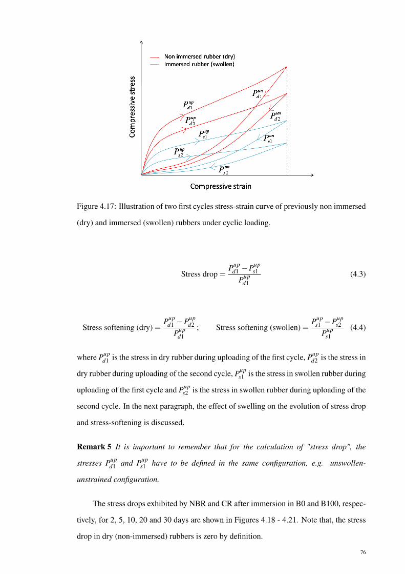
Figure 4.17: Illustration of two first cycles stress-strain curve of previously non immersed
(dry) and immersed (swollen) rubbers under cyclic loading.
Stress drop =Pup
d1 −Pups1
Pupd1
(4.3)
Stress softening (dry) =Pup
d1 −Pupd2
Pupd1
; Stress softening (swollen) =Pup
s1 −Pups2
Pups1
(4.4)
where Pupd1 is the stress in dry rubber during uploading of the first cycle, Pup
d2 is the stress in
dry rubber during uploading of the second cycle, Pups1 is the stress in swollen rubber during
uploading of the first cycle and Pups2 is the stress in swollen rubber during uploading of the
second cycle. In the next paragraph, the effect of swelling on the evolution of stress drop
and stress-softening is discussed.
Remark 5 It is important to remember that for the calculation of "stress drop", the
stresses Pupd1 and Pup
s1 have to be defined in the same configuration, e.g. unswollen-
unstrained configuration.
The stress drops exhibited by NBR and CR after immersion in B0 and B100, respec-
tively, for 2, 5, 10, 20 and 30 days are shown in Figures 4.18 - 4.21. Note that, the stress
drop in dry (non-immersed) rubbers is zero by definition.
76

Figure 4.18: Stress drop in NBR previously immersed in B0. Results correspond to 2, 5,
10, 20 and 30 days of immersion duration.
Figure 4.19: Stress drop in CR previously immersed in B0. Results correspond to 2, 5,
10, 20 and 30 days of immersion duration.
77

Figure 4.20: Stress drop in NBR previously immersed in B100. Results correspond to 2,
5, 10, 20 and 30 days of immersion duration.
Figure 4.21: Stress drop in CR previously immersed in B100. Results correspond to 2, 5,
10, 20 and 30 days of immersion duration.
78

As depicted in these figures, both NBR and CR experience stress drop in the presence
of liquid, either in diesel (B0) or biodiesel (B100). The stress drop appears to decrease
linearly with the applied compressive strain in the range of 10% - 40% for NBR and CR
immersed in B0 and 5% - 40% for NBR and CR immersed in B100 respectively. For given
immersion duration, stress drop in CR after immersion (either in B0 or B100) is higher
than that in NBR. As underlined by George et al. (1999), the high degree of swelling
experienced by CR as shown in Figures 4.1 and 4.2 appears to contribute significantly to
the decrease of its strength.
Concerning the stress-softening, it is observed that the stress-softening decreases
as the strain level approaches the maximum strain previously endured by the material
as classically observed in rubber under cyclic loading conditions (Diani et al., 2009).
Unlike the stress drop, an opposite trend is found in stress-softening, i.e. the presence
of liquids (swelling) decreases the stress-softening as can be seen in Figures 4.22 - 4.25.
While in the case of NBR after immersion in B0 and B100, this trend is easily observed,
in the case of CR it is less noticeable. Indeed, for relatively low compressive strains,
discrepancies are found in CR previously immersed in B100 during 5, 10 and 20 days.
While the exact reason of these discrepancies is not known, it could be attributed to the
fact that at low compressive strain, the stress Pups1 is so small that the corresponding level
of stress-softening cannot be correctly described by Equation (4.4)2.
79
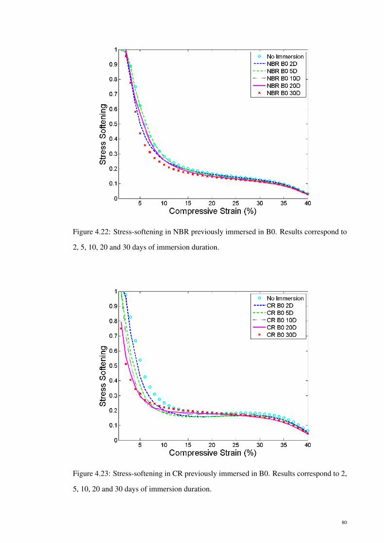
Figure 4.22: Stress-softening in NBR previously immersed in B0. Results correspond to
2, 5, 10, 20 and 30 days of immersion duration.
Figure 4.23: Stress-softening in CR previously immersed in B0. Results correspond to 2,
5, 10, 20 and 30 days of immersion duration.
80

Figure 4.24: Stress-softening in NBR previously immersed in B100. Results correspond
to 2, 5, 10, 20 and 30 days of immersion duration.
Figure 4.25: Stress-softening in CR previously immersed in B100. Results correspond to
2, 5, 10, 20 and 30 days of immersion duration.
81

4.1.2 (c) Hysteresis
The hysteresis in our materials is found to stabilize after five cycles of loading (see
Figures 4.3 and 4.4). In order to investigate the effect of swelling on hysteresis of elas-
tomers, the amount of hysteresis loss ratio at different immersion durations and different
tested fuel is investigated.
Following Bergström and Boyce (1998), the hysteresis loss ratio is calculated from
the stabilized hysteresis (after the fifth cycle). In the following, the hysteresis loss ratio is
defined by:
Hysteresis loss ratio =H5
Es(4.5)
where H5 is the amount of hysteresis (dissipated energy, given by the difference of the area
under the uploading and the unloading path of stress-strain curve) and Es is the supplied
energy during uploading (given by the area under the uploading path of the stress-strain
curve) as depicted in Figure 4.26.
Figure 4.26: Definition of hysteresis loss ratio.
Figure 4.27 depicts the hysteresis loss ratio in NBR and CR after immersion in B0
and B100 for different immersion durations. The plot clearly indicates that for both NBR
82
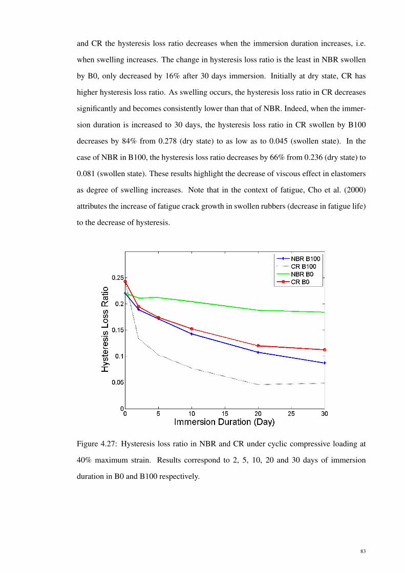
and CR the hysteresis loss ratio decreases when the immersion duration increases, i.e.
when swelling increases. The change in hysteresis loss ratio is the least in NBR swollen
by B0, only decreased by 16% after 30 days immersion. Initially at dry state, CR has
higher hysteresis loss ratio. As swelling occurs, the hysteresis loss ratio in CR decreases
significantly and becomes consistently lower than that of NBR. Indeed, when the immer-
sion duration is increased to 30 days, the hysteresis loss ratio in CR swollen by B100
decreases by 84% from 0.278 (dry state) to as low as to 0.045 (swollen state). In the
case of NBR in B100, the hysteresis loss ratio decreases by 66% from 0.236 (dry state) to
0.081 (swollen state). These results highlight the decrease of viscous effect in elastomers
as degree of swelling increases. Note that in the context of fatigue, Cho et al. (2000)
attributes the increase of fatigue crack growth in swollen rubbers (decrease in fatigue life)
to the decrease of hysteresis.
Figure 4.27: Hysteresis loss ratio in NBR and CR under cyclic compressive loading at
40% maximum strain. Results correspond to 2, 5, 10, 20 and 30 days of immersion
duration in B0 and B100 respectively.
83

4.1.2 (d) Stress-relaxation
The effect of the biodiesel diffusion on the time-dependent behavior of the elas-
tomeric materials can be probed with experiments illustrated in the inset of Figure 4.28.
Figure 4.28: Engineering stress-strain response of dry NBR under multi step relaxation
test at 0.1 mms−1 displacement rate.
In this experiment, after the specimen was pre-conditioned with six cycles of com-
pressive loading to a maximum compressive strain level of 40%, the multi-relaxation tests
at strain levels of 10, 20 and 30% were conducted during the uploading and unloading.
Similar tests were conducted for dry elastomers by Lion (1997) and Bergström and Boyce
(1998) among others. It is observed that the compressive stress decreases during the relax-
ations in the uploading and increases during the relaxations in the unloading approaching
what appears to be an equilibrium state (Bergström & Boyce, 1998) as depicted in Figure
4.28.
Further investigation of the stress relaxation is presented in Figures 4.29 to 4.32
where the normalized stress is plotted as a function of relaxation duration for different
immersion durations.
84

Figure 4.29: Stress relaxation of NBR under compressive strain levels of 30% during
1800 s. Results correspond to 2, 5, 10, 20 and 30 days of immersion in B0.
Figure 4.30: Stress relaxation CR under compressive strain levels of 30% during 1800 s.
Results correspond to 2, 5, 10, 20 and 30 days of immersion in B0.
85

Figure 4.31: Stress relaxation of NBR under compressive strain levels of 30% during
1800 s. Results correspond to 2, 5, 10, 20 and 30 days of immersion in B100.
Figure 4.32: Stress relaxation of CR under compressive strain levels of 30% during 1800
s. Results correspond to 2, 5, 10, 20 and 30 days of immersion in B100.
86

In these figures, the normalized stress is defined by the ratio between the value of
stress during relaxation at specific time, σ(t) and the maximum stress achieved at the be-
ginning of the corresponding relaxation, σo. Only stress relaxation at strain level of 30%
during uploading is presented, since the stress relaxation at other strain levels give quali-
tatively similar results. As clearly shown, the graphs in Figures 4.29 to 4.32 show similar
trends. The presence of liquids (swelling) appears to render the material under loading
to become closer to the equilibrium state, i.e. the viscous (time-dependent) contribution
to the macroscopic mechanical response of material becomes smaller which is consistent
with the results of the hysteresis discussed in the previous subsection. Indeed, after 1800
s of relaxation, the stress decreases by the amount of 16% for dry NBR and by 6% when
the specimen is immersed in B100 for 30 days. While for CR, the stress only decreases
by 3% after immersion for 30 days whereas the stress in dry CR decreased by 17% after
1800 s of relaxation. In the case of NBR after 30 days of immersion in B0, the stress de-
cays the most, to 11% showing that the viscous effect in the rubber is still preserved. As
emphasized by Radhakrishnan Nair (1997); Wypych (2004), the palm biodiesel appears
to act as lubricant facilitating movement of the polymer chain segments. The distances
between the molecules become lesser (physical bonds become weaker).
4.1.3 SEM results
Figure 4.33 shows the micrographs of the cross sectional surface of the dry and
swollen elastomers after immersion in B0 and B100 for 5 days and 30 days, respectively.
The cross sectional surface of swollen CR shows larger voids than swollen NBR and dry
CR and NBR.
NBR in diesel shows an insignificant effect compared to those in B100. Larger voids
were found in NBR and CR after swollen in biodiesel. As pointed out by Ismail, Nordin,
and Noor (2002), weak filler-matrix interaction is indicated by the presence of many
holes or loose fillers on the cross-sectional surface as shown by swollen CR in B100.
On the other hand, the void formation could be the result of the introduction of polar
oxygen groups into elastomers or cross-linking or macromolecule chain scission (Haseeb
et al., 2010). The microstructural changes can be attributed to the increasing surface
energy, subsequently leading to localized decreases or increases in density, which will
87

cause the creation of voids, cracks or pits. In addition, freezing a large amount of stress
energy in the polymer can cause crack formation in the rubber (Miller-Chou & Koenig,
2003). According to Ueberreiter (1968), elastomer can be dissolved in solvent either by
exhibiting a thick swollen layer or by undergoing extensive cracking, depending on the
osmotic pressure stress release rate that builds up in the polymer matrix. In other words,
elastomers that exhibit more swelling or cracking tend to dissolve during immersion.
Therefore, nitrile rubber and polychloroprene show more cracks and voids in B100 than
in B0 due to higher solubility in palm biodiesel.
88

Figure 4.33: SEM images of the cross sectional surface of the dry and swollen elastomers
after immersed in B0 and B100 for 5 and 30 days respectively, X500.
89

4.2 Results of swelling tests on uniaxially-stressed specimens
4.2.1 Mass and volume changes
To determine the effect of static mechanical loading on swelling behavior of NBR
and CR specimens, the swelling test is conducted by initially constrained the specimens
at different compressive strains using a compression device and subsequently immersing
into different biodiesel blends for 30 and 90 days. Figures 4.34 to 4.41 show the per-
centage of mass change and volume change of NBR and CR with different compressive
strains (2%, 10% and 20%) after immersion in different biodiesel blends (B0, B25, B75
and B100) for 30 and 90 days respectively.
Figure 4.34: Mass change of NBR at different compressive strains after 30 days immer-
sion in different percentage of biodiesel blends.
90

Figure 4.35: Volume change of NBR at different compressive strains after 30 days im-
mersion in different percentage of biodiesel blends.
Figure 4.36: Mass change of NBR at different compressive strains after 90 days immer-
sion in different percentage of biodiesel blends.
91

Figure 4.37: Volume change of NBR at different compressive strains after 90 days im-
mersion in different percentage of biodiesel blends.
Figure 4.38: Mass change of CR at different compressive strains after 30 days immersion
in different percentage of biodiesel blends.
92

Figure 4.39: Volume change of CR at different compressive strains after 30 days immer-
sion in different percentage of biodiesel blends.
Figure 4.40: Mass change of CR at different compressive strains after 90 days immersion
in different percentage of biodiesel blends.
93

Figure 4.41: Volume change of CR at different compressive strains after 90 days immer-
sion in different percentage of biodiesel blends.
All the plots show similar patterns. Both NBR and CR show increases in mass and
volume change when the exposure time is increased from 30 to 90 days. The percentage
of fuel uptake is increasing with the increase of palm biodiesel content. It is clear that for
low biodiesel content (B0 and B25) no significant fuel uptake (less than 10% mass and
volume change) is recorded for NBR. At higher percentage of biodiesel content (B100),
both NBR and CR show significant mass and volume change. The corresponding trend
can be attributed to the segmental mobility of the polymer and free volume of the polymer
(George & Thomas, 2001).
Generally, it is also observed that the fuel uptake is affected by the level of pre-
compression. The increase of pre-compressive strain has restricted the fuel uptake into
the elastomeric material, i.e. the compressive stress appears to reduce the amount of
swelling compared to that for stress-free rubber. As the compressive strain increases, the
effective area for diffusion to occur along the radial direction in hollow cylindrical rubber
specimens becomes smaller. Hence, the resulting swelling is lower. Furthermore, the
reduction in swelling of rubber is affected by the hydrostatic component of the applied
94

stress (Treloar, 1975; Fukumori et al., 1990). According to the authors, a compressive
stress, for which the hydrostatic components is positive, leads to a decrease in the swelling
of rubber. In the next subsection, only results that correspond to 2% pre-compressive
strain are presented since the pre-compressive strain of 2% yields the highest degree of
swelling.
4.2.2 Mechanical response
The stress-strain curves of dry and swollen NBR and CR under cyclic compressive
loading at two different maximum compressive strains are illustrated in Figures 4.42 and
4.43. For each maximum compressive strain, the specimen experiences six cycles of
loading. It is shown that there is not much difference in the nature of stress-strain behav-
ior after immersion. However, lower stress is recorded for CR after 90 days immersion
given the same pre-compressive strain. The corresponding behavior can be related to the
swelling in the CR which decreases its strength due to strong interaction of rubber-solvent
matrix system (George et al., 1999).
Under cyclic loading conditions, both dry NBR and CR exhibit significant inelastic
responses, i.e. mechanical hysteresis and stress-softening. Though a number of works
are devoted to the understanding of this stress-softening, no general agreement has been
reached either on the physical source or on the mechanical modeling of this softening
at the microscopic or meso-scopic scales (Diani et al., 2009). Similar to the observa-
tion from stress-free swollen specimens, when uniaxially-stressed NBR and CR are in
swollen state, the above inelastic responses decrease significantly, i.e. smaller hysteresis
and stress-softening are observed. The following paragraphs focus only on stress re-
sponses that correspond to maximum cyclic compressive strain of 30% since the data at
larger strain shows similar trend.
95

Figure 4.42: Stress-strain curves of NBR at dry states (without immersion) and after 30
days (1M) and 90 days (3M) immersion in B100. Results correspond to pre-compressive
strain of 2%. For immersed rubbers, the stress is expressed with respect to the swollen-
unstrained configuration (initial swollen cross section).
Figure 4.43: Stress-strain curves of CR at dry states (without immersion) and after 30
days (1M) and 90 days (3M) immersion in B100. Results correspond to pre-compressive
strain of 2%. For immersed rubbers, the stress is expressed with respect to the swollen-
unstrained configuration (initial swollen cross section).
96

4.2.2 (a) Nature of swelling
Following the methods used to evaluate the nature of swelling of stress-free spec-
imens proposed in Section 4.1.2 (a), the five methods are compared using stress-strain
data obtained from uniaxially-stressed swollen rubbers. In Figures 4.44 to 4.47, the shear
modulus ratios obtained using M-1, M-2 and M-3 methods are plotted as a function of
applied compressive strain for NBR and CR immersed in B0 and B100 respectively. In
each graph, results that correspond to 30 days (1M) and 90 days (3M) immersion are pre-
sented. Similarly, in Figures 4.48 to 4.51, shear modulus ratios are plotted, but this time
using M-1, M-4 and M-5 methods.
Figure 4.44: Shear modulus ratio obtained using M-1, M-2 and M-3 methods as a function
of applied compressive strain for NBR after immersion in B0. Results correspond to 2%
pre-compressive strain.
97

Figure 4.45: Shear modulus ratio obtained using M-1, M-2 and M-3 methods as a function
of applied compressive strain for CR after immersion in B0. Results correspond to 2%
pre-compressive strain.
Figure 4.46: Shear modulus ratio obtained using M-1, M-2 and M-3 methods as a function
of applied compressive strain for NBR after immersion in B100. Results correspond to
2% pre-compressive strain.
98

Figure 4.47: Shear modulus ratio obtained using M-1, M-2 and M-3 methods as a function
of applied compressive strain for CR after immersion in B100. Results correspond to 2%
pre-compressive strain.
Figure 4.48: Shear modulus ratio obtained using M-1, M-4 and M-5 methods as a function
of applied compressive strain for NBR after immersion in B0. Results correspond to 2%
pre-compressive strain.
99

Figure 4.49: Shear modulus ratio obtained using M-1, M-4 and M-5 methods as a function
of applied compressive strain for CR after immersion in B0. Results correspond to 2%
pre-compressive strain.
Figure 4.50: Shear modulus ratio obtained using M-1, M-4 and M-5 methods as a function
of applied compressive strain for NBR after immersion in B100. Results correspond to
2% pre-compressive strain.
100

Figure 4.51: Shear modulus ratio obtained using M-1, M-4 and M-5 methods as a function
of applied compressive strain for CR after immersion in B100. Results correspond to 2%
pre-compressive strain.
Similar to the results obtained from the stress-free swollen rubbers, as depicted in
Figures 4.44 to 4.51, it is found that the shear modulus ratio deviates from the cube root
of the swelling ratio as predicted by Treloar, i.e. results obtained using M-2, M-3, M-4
and M-5 methods are different from those obtained from M-1. Regardless of the type
of rubber and the method considered, qualitatively similar results are obtained from the
uniaxially-stressed swollen rubbers:
1. The deviation from Treloar theory in the shear modulus ratio resulting from im-
mersion in B100 is systematically larger than the one resulting from immersion in
B0.
2. Increasing the duration of immersion from 1 month to 3 months increases the cor-
responding deviation.
3. The shear modulus ratios calculated using the estimated equilibrium stress response,
i.e. M-4 and M-5, appear to give closer values to the one predicted by Treloar than
using the first uploading stress response, i.e. M-2 and M-3.
101

4.2.2 (b) Stress drop
Using Equation 4.3, the stress drops for the uniaxially-stressed specimens is calcu-
lated. Figures 4.52 to 4.55 show the stress drop exhibited by NBR and CR after immersion
in various biodiesel blends for 1 month (1M) and 3 months (3M).
Figure 4.52: Stress drop in NBR previously immersed in various biodiesels for 1 month
(1M). Results correspond to pre-compressive strain of 2%.
102

Figure 4.53: Stress drop in NBR previously immersed in various biodiesels for 3 months
(3M). Results correspond to pre-compressive strain of 2%.
Figure 4.54: Stress drop in CR previously immersed in various biodiesels for 1 month
(1M). Results correspond to pre-compressive strain of 2%.
103
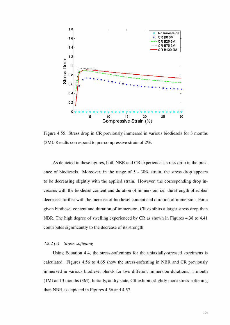
Figure 4.55: Stress drop in CR previously immersed in various biodiesels for 3 months
(3M). Results correspond to pre-compressive strain of 2%.
As depicted in these figures, both NBR and CR experience a stress drop in the pres-
ence of biodiesels. Moreover, in the range of 5 - 30% strain, the stress drop appears
to be decreasing slightly with the applied strain. However, the corresponding drop in-
creases with the biodiesel content and duration of immersion, i.e. the strength of rubber
decreases further with the increase of biodiesel content and duration of immersion. For a
given biodiesel content and duration of immersion, CR exhibits a larger stress drop than
NBR. The high degree of swelling experienced by CR as shown in Figures 4.38 to 4.41
contributes significantly to the decrease of its strength.
4.2.2 (c) Stress-softening
Using Equation 4.4, the stress-softenings for the uniaxially-stressed specimens is
calculated. Figures 4.56 to 4.65 show the stress-softening in NBR and CR previously
immersed in various biodiesel blends for two different immersion durations: 1 month
(1M) and 3 months (3M). Initially, at dry state, CR exhibits slightly more stress-softening
than NBR as depicted in Figures 4.56 and 4.57.
104

Figure 4.56: Stress-softening in NBR and CR previously immersed in B0 for two different
durations of immersion: 1 month (1M) and 3 months (3M). Results correspond to pre-
compressive strain of 2%.
Figure 4.57: Stress-softening in NBR and CR previously immersed in B100 for two dif-
ferent durations of immersion: 1 month (1M) and 3 months (3M). Results correspond to
pre-compressive strain of 2%.
105

Nevertheless, as the material is immersed for 1 month in either B0 or B100, the
stress-softening decreases significantly in CR and becomes lower than that of NBR. In
NBR, for a compressive strain of 10%, the amount of stress-softening drops from 20% at
dry state to 18% and 15% at swollen state (immersed in B0 and B100 respectively for 1
month) as presented in Figures 4.58 and 4.59.
Figure 4.58: Stress-softening in NBR previously immersed in B0 for two different du-
rations of immersion: 1 month (1M) and 3 months (3M). Results correspond to pre-
compressive strain of 2%.
106

Figure 4.59: Stress-softening in NBR previously immersed in B100 for two different
durations of immersion: 1 month (1M) and 3 months (3M). Results correspond to pre-
compressive strain of 2%.
Increasing the duration of immersion from 1 to 3 months yields a further decrease of
stress-softening to around 15% and 12% in B0 and B100 respectively. Referring to Fig-
ures 4.35 and 4.37, this corresponds to the volume change of 11% and 18% respectively.
In the case of CR, at an applied compressive strain of 10%, the amount of stress-
softening changes from 28% for dry state to only 12% and 8% when it is immersed
respectively in B0 and B100 for 1 month as shown in Figures 4.60 and 4.61. Note that in
the latter condition, the volume change exhibited by the material is around 18% and 64%
respectively (see Figures 4.39 and 4.41).
107

Figure 4.60: Stress-softening in CR previously immersed in B0 for two different durations
of immersion: 1 month (1M) and 3 months (3M). Results correspond to pre-compressive
strain of 2%.
Figure 4.61: Stress-softening in CR previously immersed in B100 (right) for two different
durations of immersion: 1 month (1M) and 3 months (3M). Results correspond to pre-
compressive strain of 2%.
108

Increasing the duration of immersion from 1 to 3 months yields a significant increase
in the volume change to around 24% and 90% in B0 and B100 respectively. However, the
level of stress-softening appears to be unaffected by the corresponding further increase
in swelling. Finally, the effect of biodiesel content on stress-softening in NBR and CR is
presented in Figures 4.62 to 4.65. In these figures, it is found that for both materials, the
increase in the content of biodiesel decreases the level of stress-softening.
Figure 4.62: Stress-softening in NBR previously immersed in various biodiesels for 1
month (1M). Results correspond to pre-compressive strain of 2%.
109

Figure 4.63: Stress-softening in NBR previously immersed in various biodiesels for 3
months (3M). Results correspond to pre-compressive strain of 2%.
Figure 4.64: Stress-softening in CR previously immersed in various biodiesels for 1
month. Results correspond to pre-compressive strain of 2%.
110
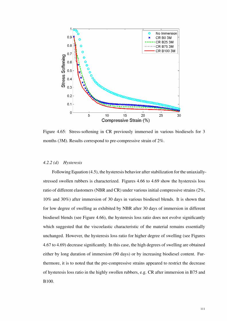
Figure 4.65: Stress-softening in CR previously immersed in various biodiesels for 3
months (3M). Results correspond to pre-compressive strain of 2%.
4.2.2 (d) Hysteresis
Following Equation (4.5), the hysteresis behavior after stabilization for the uniaxially-
stressed swollen rubbers is characterized. Figures 4.66 to 4.69 show the hysteresis loss
ratio of different elastomers (NBR and CR) under various initial compressive strains (2%,
10% and 30%) after immersion of 30 days in various biodiesel blends. It is shown that
for low degree of swelling as exhibited by NBR after 30 days of immersion in different
biodiesel blends (see Figure 4.66), the hysteresis loss ratio does not evolve significantly
which suggested that the viscoelastic characteristic of the material remains essentially
unchanged. However, the hysteresis loss ratio for higher degree of swelling (see Figures
4.67 to 4.69) decrease significantly. In this case, the high degrees of swelling are obtained
either by long duration of immersion (90 days) or by increasing biodiesel content. Fur-
thermore, it is to noted that the pre-compressive strains appeared to restrict the decrease
of hysteresis loss ratio in the highly swollen rubbers, e.g. CR after immersion in B75 and
B100.
111
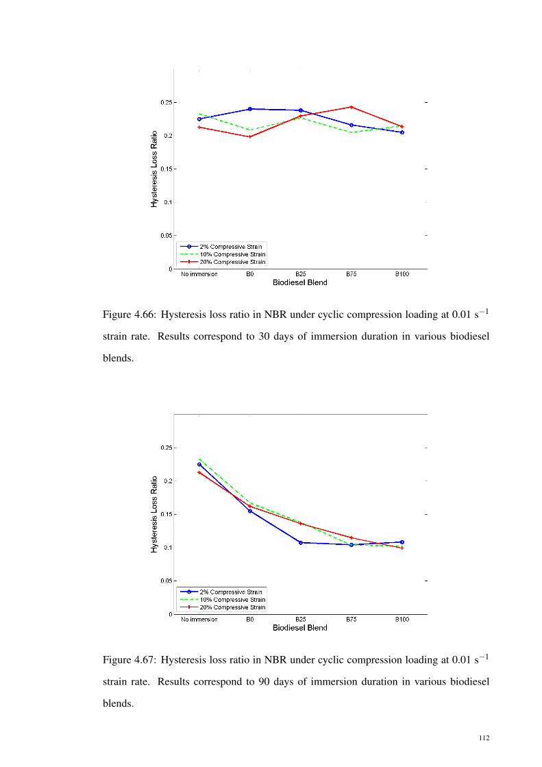
Figure 4.66: Hysteresis loss ratio in NBR under cyclic compression loading at 0.01 s−1
strain rate. Results correspond to 30 days of immersion duration in various biodiesel
blends.
Figure 4.67: Hysteresis loss ratio in NBR under cyclic compression loading at 0.01 s−1
strain rate. Results correspond to 90 days of immersion duration in various biodiesel
blends.
112

Figure 4.68: Hysteresis loss ratio in CR under cyclic compression loading at 0.01 s−1
strain rate. Results correspond to 30 days of immersion duration in various biodiesel
blends.
Figure 4.69: Hysteresis loss ratio in CR under cyclic compression loading at 0.01 s−1
strain rate. Results correspond to 90 days of immersion duration in various biodiesel
blends.
113

4.2.2 (e) Stress Relaxation
Following the description in Section 4.1.2 (d) in Chapter 4, the stress relaxation for
NBR and CR in different biodiesel blends at 30% compressive strain during uploading
is reported in Figures 4.70 to 4.73. The curves reveal that the stress relaxation occurs
rapidly during the first 200 seconds but subsequently becomes slower as indicated by the
near-horizontal curve. Moreover, one can notice that stress relaxation is reducing with
the increase of biodiesel content. This suggests that the biodiesel content has a significant
influence on the viscoelastic response.
To close the discussion, note that all inelastic phenomena, e.g. stress-softening and
mechanical hysteresis, in rubbers resulting from cyclic loading conditions appear to di-
minish significantly due to the presence of liquids, i.e. the macroscopic mechanical re-
sponse of swollen rubbers approaches the response of hyperelastic materials. Neverthe-
less, the physical mechanism by which the presence of liquids modify the mechanical
response under the above loading condition remains unknown.
Figure 4.70: Stress relaxation of NBR under compressive strain levels of 30% during
1800 s. Results correspond to 2% pre-compressive strain and 30 days of immersion in
various biodiesel blends.
114

Figure 4.71: Stress relaxation of NBR under compressive strain levels of 30% during
1800 s. Results correspond to 2% pre-compressive strain and 90 days of immersion in
various biodiesel blends.
Figure 4.72: Stress relaxation of CR under compressive strain levels of 30% during 1800
s. Results correspond to 2% pre-compressive strain and 30 days of immersion in various
biodiesel blends.
115

Figure 4.73: Stress relaxation of CR under compressive strain levels of 30% during 1800
s. Results correspond to 2% pre-compressive strain and 90 days of immersion in various
biodiesel blends.
4.3 Comparison between experimental results of swelling tests on stress-free anduniaxially-stressed specimens
Comparing the swelling results between the stress-free and uniaxially stressed spec-
imens, it is found that the pre-compressive strains restrict the swelling in the uniaxially-
stressed specimens. Although the immersion durations varied between these two tests,
the swelling results are qualitatively similar. Concerning the mechanical responses, the
effect of pre-compressive strain during immersion on the resulting mechanical responses
is not significant. This could be due to the fact that the swelling between the three pre-
compressive strains (2%, 10% and 30%) imposed is not significant to cause the degree
of swelling to vary significantly. As such, comparing the mechanical responses, i.e. the
stress-softening, hysteresis, stress-relaxation between the stress-free swollen rubbers with
the highest degree of swelling in the uniaxially stressed swollen rubbers, relatively sim-
ilar results are obtained. We can conclude here that the higher the degree of swelling,
whether it is due to higher biodiesel content, longer immersion duration, or lower level
of pre-compressive strain, the more the inelastic responses, i.e. the stress-softening, hys-
teresis, stress-relaxation are reduced.
116

CHAPTER 5
MODELING RESULTS AND DISCUSSION
As we have seen in Chapter 4, the mechanical responses of swollen rubber are complex,
and include the responses of stress-softening, hysteresis, stress-relaxation, etc. To simu-
late the real engineering components in the swollen state, an efficient model taking into
account all the observed inelastic responses is required. The development of such model
is complex. As a first attempt, only the modeling of the Mullins effect is considered. This
chapter presents the modeling results and compares them with the experimental results
for stress-softening in swollen rubbers. Furthermore, the three-dimensional nature of the
model in capturing the effect of swelling on the stress-softening due to Mullins effect is
illustrated in simulations of uniaxial tension, pure shear and equibiaxial tension.
5.1 Data treatment
Since the Mullins effect is the only inelastic response addressed in the continuum
mechanical modeling, the results in Figures 4.3 and 4.4 have to be treated. More pre-
cisely, only the Mullins effect which occurs between the first and second loading cycles
is considered. For this purpose, the data treatment proposed by Chagnon et al. (2004)
is considered: (i) the reloading path of the second cycle is assumed to coincide with the
downloading path of the first cycle, (ii) the unloading data are horizontally shifted such
that they start from zero strain and (iii) the unloading data are extended to rejoin the pri-
mary loading path. An example of the comparison between original and corrected data in
CR is depicted in Figures 5.1 and 5.2.
117

Figure 5.1: Experimental results for dry CR under cyclic compressive test.
Figure 5.2: Modified data for dry CR under cyclic compressive test.
118

5.2 Flory-Huggins interaction parameters, χ
To obtain the parameter χ for different rubber-solvent combinations, we first need to
determine the volume of the solvent molecules, ν .
The volume of the solvent molecules ν is given by:
ν =Mw
ρAv(5.1)
where,
Mw is the molecular weight of the solvent,
ρ is the density of the solvent,
Av is the Avogadro number, which is equal to 6.022.1023 /mol.
The molecular weight of the diesel is obtained from the bibliography. While the
molecular weight of the palm biodiesel is approximated from the chemical content of the
biodiesel. Detailed calculation is shown in Table 5.1
Table 5.1: Biodiesel molecular weight calculation.
Chemicals Molecules C H O Molecular weight % in biodiesel
Methyl Laurate CH3(CH2)10COOCH3 12 26 2 214 1.066 2.281
Methyl Myristate CH3(CH2)12COOCH3 15 30 2 242 3.700 8.954
Methyl Palmitate CH3(CH2)14COOCH3 17 34 2 270 44.272 119.534
Methyl Palmitoleate CH3(CH2)5CHCH(CH2)7COOCH3 17 30 2 266 0.497 1.322
Methyl Stearate CH3(CH2)16COOCH3 19 38 2 298 4.128 12.301
Methyl Oleate CH3(CH2)7CHCH(CH2)7COOCH3 19 36 2 296 35.934 106.365
Methyl Arachisate CH3(CH2)18COOCH3 21 42 2 326 0.236 0.769
Total chemical content 89.833 % 251.527
Estimated Molecular weight 100 % 280
The volume of the B0 and B100 molecules is then determined using Equation 5.1.
The calculation is shown in Table 5.2
119

Table 5.2: The volume of the B0 and B100 molecules.
B0 B100
Molecular weight (g/mol) 280 198.4
Density (g/m3) 875900 878800
Avogadro number 6.02x10²³ 6.02x10²³
The volume of the solvent molecules (m3) 5.31x10⁻²⁸ 3.75x10⁻²⁸
Assuming equilibrium swelling occurred after 30 days of immersion for NBR and
CR in B0 and B100 and recalling Equation (3.3), the Flory-Huggins Interaction parame-
ter, χ is then calculated using Matlab. The results are shown in Table 5.3.
Table 5.3: Flory-Huggins interaction parameter χ of each rubber-fuel system.
χCR−B100 0.311
χCR−B0 1.356
χNBR−B100 1.285
χNBR−B0 1.767
5.3 Extended pseudo-elastic model
5.3.1 Form of material functions
In order to describe the general response of swollen rubbers, a simple neo-Hookean
hyperelastic strain energy density is retained:
Wm(Js, I1m) =µ(Js)
2(I1m−3) (5.2)
where µ(Js) is the shear modulus of swollen rubber. According to Treloar (1975), swelling
in rubber is a purely mixing or interdiffusion process with no chemical attraction between
rubber and liquid molecules. Furthermore, the only effect of swelling is to reduce the
modulus in inverse proportion to the cube root of the degree of swelling without chang-
ing the form of the stress-strain curves. Generalizing this idea, the shear modulus of the
120

swollen rubber µ(Js) is assumed to be related to that of dry rubber µd through:
µ(Js) = J−ns µd (5.3)
It follows that the strain energy function of the swollen rubber becomes
Wm(Js, I1m) = J−ns
µd
2(I1m−3) (5.4)
where n is a parameter to be determined from all sets of experimental data. In this case,
the engineering stress in Eq. (3.44) reduces to:
P11 = J−ns µd (1−d)
(λm−
1λ 2
m
)(5.5)
where d is given in Eq. (3.39).
In order to determine the explicit forms of r (Js,χ) and m(Js,χ), the experimental
data as shown in Figure 5.2 are considered. More precisely, the experimental values of
damage d are plotted as a function of I1m,max− I1m. The results for CR swollen by B0 and
B100 are depicted in Figures 5.3 and 5.4 .
121
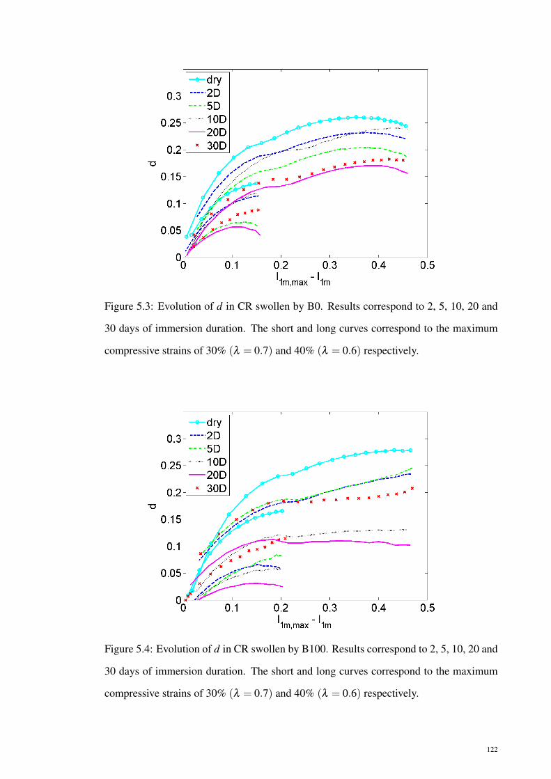
Figure 5.3: Evolution of d in CR swollen by B0. Results correspond to 2, 5, 10, 20 and
30 days of immersion duration. The short and long curves correspond to the maximum
compressive strains of 30% (λ = 0.7) and 40% (λ = 0.6) respectively.
Figure 5.4: Evolution of d in CR swollen by B100. Results correspond to 2, 5, 10, 20 and
30 days of immersion duration. The short and long curves correspond to the maximum
compressive strains of 30% (λ = 0.7) and 40% (λ = 0.6) respectively.
122

Note that the corresponding results for NBR swollen by B0 and B100 are not shown
since they are qualitatively similar. In the Figures 5.3 and 5.4, d is obtained from the
following expressions:
d(dry) =Pup
d1 −Pund1
Pupd1
d(swollen) =Pup
s1 −Puns1
Pups1
(5.6)
where Pupd1 is the stress in dry rubber during uploading of the first cycle, Pun
d1 is the stress
in dry rubber during unloading of the first cycle, Pups1 is the stress in swollen rubber dur-
ing uploading of the first cycle and Puns1 is the stress in swollen rubber during unloading
of the first cycle. It is generally observed that the damage is strongly affected by the
degree of swelling and the type of rubber-solvent, i.e. interaction between rubber and
biodiesel/diesel. More precisely, the Mullins effect appears to decrease with the increase
of degree of swelling.
By considering the initial slope and the maximum value of d in Figures 5.3 and 5.4,
and recalling the discussion on the last paragraph of Section 3.2.4 (a), it is possible to plot
the evolution of both m and r as a function of χ (Js−1) as shown in Figures 5.5 and 5.6.
Figure 5.5: Evolution of r as a function of χ (Js−1). Results correspond to the maximum
compressive strain of 40%.
123

Figure 5.6: Evolution of m as a function of χ (Js−1). Results correspond to the maxi-
mum compressive strain of 40%.
In general, it is observed that both r and m are increasing functions of χ (Js−1).
Motivated by this finding, and for the sake of simplicity, the parameters r and m are
assumed to evolve in a simple linear way as follow:
r = rd +∆r ·χ (Js−1) m = md +∆m ·χ (Js−1) . (5.7)
where rd and md are the values of r and m for dry rubbers. ∆r and ∆m are additional
material constants. Finally, the damage function d in Eq. (3.39) becomes:
d =1
rd +∆r ·χ (Js−1)erf[
1md +∆m ·χ (Js−1)
(I1m,max− I1m)
]. (5.8)
To summarize, the following parameters in Table 5.4 have to be identified:
124

Table 5.4: Summary of material parameters required in the proposed model.
Hyperelasticity (neo-Hookean) µd
Mullins-effect rd md
Swelling n ∆r ∆m
5.3.2 Identification of material parameters
In the following, methods to estimate the material parameters of the model are dis-
cussed. The parameter µd can be obtained by fitting the primary curve of dry rubber using
the Neo-Hookean hyperelastic strain energy while rd and md can be identified from the
set of secondary curves (downloading) of dry rubber. The power law parameter n, can
be estimated by considering the primary curve of dry rubber and primary curves of cor-
responding swollen rubbers having different degrees of swelling. The parameters ∆r and
∆m can be estimated by considering the slope of the data in Figures 5.5 and 5.6 respec-
tively. Since the slopes of r and m do not vary significantly for different rubber-solvent
combinations, the values of ∆r and ∆m are assumed to be independent of the types of
rubber and solvent and their estimated values are illustrated by dashed lines in Figures
5.5 and 5.6 respectively. Finally, the estimated parameters are summarized in Table 5.5:
Table 5.5: Values of material parameters used in model.
NBR CR
µd (MPa) 1.7786 1.9102
rd 4.4340 3.4182
md 0.2720 0.1683
n 2.5
∆r 4.2
∆m 0.8
5.3.3 Comparison between model and experiment
The ability of the proposed model to describe Mullins effect in swollen rubbers under
cyclic compressive loading conditions is presented in Figures 5.7-5.28. For comparison,
125
the results related to the dry rubber are also shown in the figure.
In general, it is observed that the proposed model is qualitatively in good agreement
with experiments. The primary curves of dry and swollen rubbers are well-described.
Moreover, the effects of swelling on the stress-softening due to Mullins effect are well-
predicted. Some discrepancies between model and experiments are found for swollen
rubbers having relatively high degree of swelling. Indeed, as shown in Figures 5.13 to
5.23, the model appears to slightly underestimate the stress level in highly swollen rub-
bers. Furthermore, for the case of CR swollen by B100, the stress level and Mullins effect
predicted by the model are significantly smaller than the ones obtained from the exper-
iments as presented in Figures 5.24 to 5.28 . The corresponding discrepancies could be
attributed to the value of parameters ∆r and ∆m used in the present model. Indeed, for
the sake of simplicity, they are chosen to be independent of the rubber type and rubber-
solvent combination. Furthermore, it was also assumed that Treloar’s theory holds for all
swollen rubbers (Treloar, 1975), i.e. there is no chemical attraction between rubber and
solvent molecules in swollen rubbers. While this assumption appears to be acceptable for
relatively low degree of swelling, its validity in the case of highly swollen rubber such as
CR in B100 becomes questionable. Indeed, as discussed in Haseeb et al. (2011), chemical
reaction and interaction occurs between the B100 molecules and CR backbone resulting
to the degradation of its mechanical properties.
126

Figure 5.7: Comparison between pseudo-elastic model and experiment for dry NBR.
Figure 5.8: Comparison between pseudo-elastic model and experiment for NBR swollen
by B0 after 2 days immersion (χ = 1.7669).
127

Figure 5.9: Comparison between pseudo-elastic model and experiment for NBR swollen
by B0 after 5 days immersion (χ = 1.7669).
Figure 5.10: Comparison between pseudo-elastic model and experiment for NBR swollen
by B0 after 10 days immersion (χ = 1.7669).
128
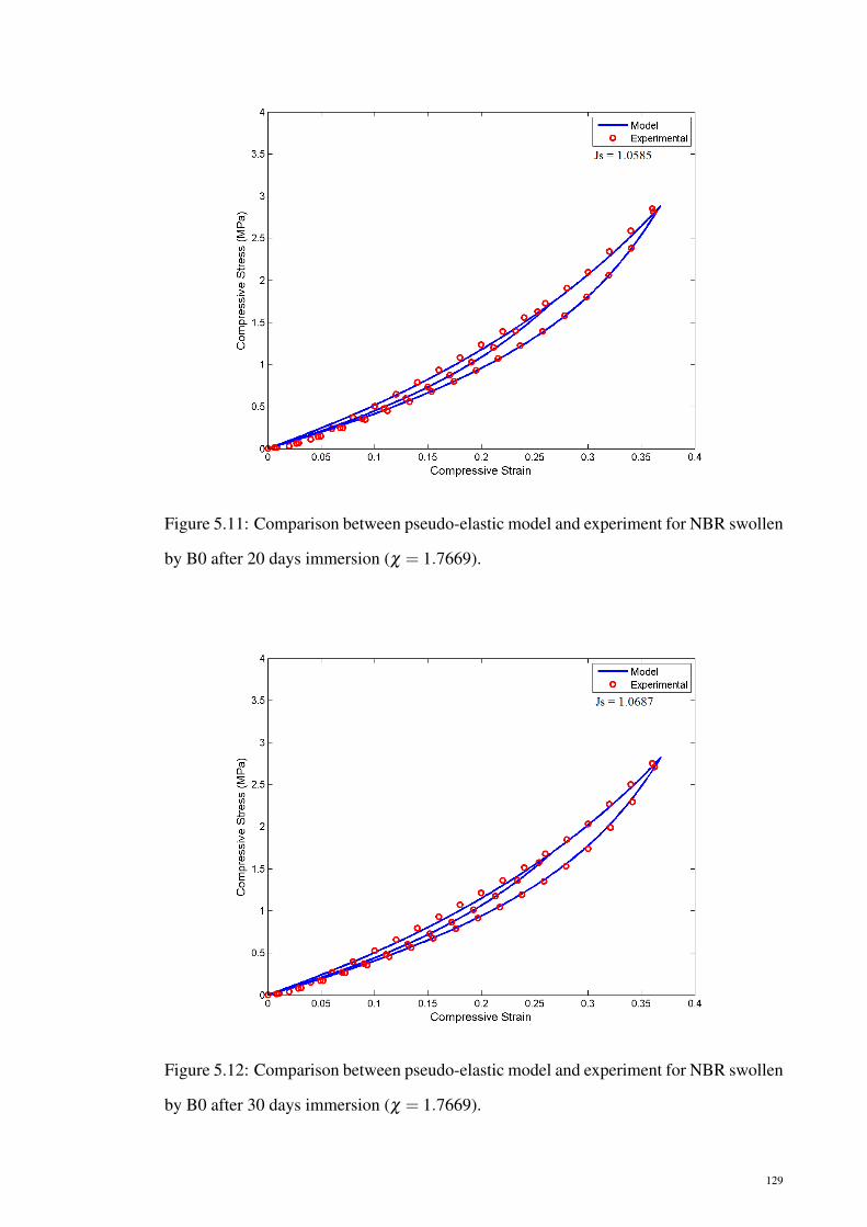
Figure 5.11: Comparison between pseudo-elastic model and experiment for NBR swollen
by B0 after 20 days immersion (χ = 1.7669).
Figure 5.12: Comparison between pseudo-elastic model and experiment for NBR swollen
by B0 after 30 days immersion (χ = 1.7669).
129

Figure 5.13: Comparison between pseudo-elastic model and experiment for NBR swollen
by B100 after 2 days immersion (χ = 1.2855).
Figure 5.14: Comparison between pseudo-elastic model and experiment for NBR swollen
by B100 after 5 days immersion (χ = 1.2855).
130

Figure 5.15: Comparison between pseudo-elastic model and experiment for NBR swollen
by B100 after 10 days immersion (χ = 1.2855).
Figure 5.16: Comparison between pseudo-elastic model and experiment for NBR swollen
by B100 after 20 days immersion (χ = 1.2855).
131

Figure 5.17: Comparison between pseudo-elastic model and experiment for NBR swollen
by B100 after 30 days immersion (χ = 1.2855).
Figure 5.18: Comparison between pseudo-elastic model and experiment for dry CR.
132

Figure 5.19: Comparison between pseudo-elastic model and experiment for CR swollen
by B0 after 2 days immersion (χ = 1.3561).
Figure 5.20: Comparison between pseudo-elastic model and experiment for CR swollen
by B0 after 5 days immersion (χ = 1.3561).
133

Figure 5.21: Comparison between pseudo-elastic model and experiment for CR swollen
by B0 after 10 days immersion (χ = 1.3561).
Figure 5.22: Comparison between pseudo-elastic model and experiment for CR swollen
by B0 after 20 days immersion (χ = 1.3561).
134

Figure 5.23: Comparison between pseudo-elastic model and experiment for CR swollen
by B0 after 30 days immersion (χ = 1.3561).
Figure 5.24: Comparison between pseudo-elastic model and experiment for CR swollen
by B100 after 2 days immersion (χ = 0.3113).
135

Figure 5.25: Comparison between pseudo-elastic model and experiment for CR swollen
by B100 after 5 days immersion (χ = 0.3113).
Figure 5.26: Comparison between pseudo-elastic model and experiment for CR swollen
by B100 after 10 days immersion (χ = 0.3113).
136

Figure 5.27: Comparison between pseudo-elastic model and experiment for CR swollen
by B100 after 20 days immersion (χ = 0.3113).
Figure 5.28: Comparison between pseudo-elastic model and experiment for CR swollen
by B100 after 30 days immersion (χ = 0.3113).
137

5.3.4 Simulation for other deformation modes
To simulate the response of the extended pseudo-elastic model under multiaxial load-
ing conditions, deformation modes of uniaxial extension, pure shear and equibiaxial ex-
tension are considered in the following. The material is simulated to undergo cyclic load-
ing to two maximum strain levels: ε=0.25 and 0.50. Using the material parameters fitted
from the extended pseudo-elastic model under uniaxial compression test results, different
degrees of swelling are considered in the simulation. For illustration purpose, only NBR
swollen in B0 and B100 for 10 and 20 days and CR swollen in B0 and B100 for 5 and 10
days are simulated.
5.3.4 (a) Uniaxial extension
Simulation of uniaxial extension loading-unloading curves For uniaxial extension,
the governing equation needed is given by:
P11 = J−ns µd (1−d)
(λm−
1λ 2
m
)(5.9)
where λm is the uniaxial extension stretch. The uniaxial extension loading-unloading
curves simulated with extended pseudo-elastic model are illustrated in Figures 5.29 to
5.38.
From these figures, it is clearly shown that the proposed extended pseudo-elastic
model well predicts that the uniaxial extension loading-unloading curves are affected by
the degree of swelling, i.e. lower stress level is produced for rubbers experiencing higher
degree of swelling. Furthermore, smaller stress-softening is well predicted when the de-
gree of swelling increases.
138

Figure 5.29: Pseudo-elastic model response under uniaxial extension for dry NBR.
Figure 5.30: Pseudo-elastic model response under uniaxial extension for NBR swollen
by B0 after 10 days immersion.
139

Figure 5.31: Pseudo-elastic model response under uniaxial extension for NBR swollen
by B0 after 20 days immersion.
Figure 5.32: Pseudo-elastic model response under uniaxial extension for NBR swollen
by B100 after 10 days immersion.
140

Figure 5.33: Pseudo-elastic model response under uniaxial extension for NBR swollen
by B100 after 20 days immersion.
Figure 5.34: Pseudo-elastic model response under uniaxial extension for dry CR.
141

Figure 5.35: Pseudo-elastic model response under uniaxial extension for CR swollen by
B0 after 5 days immersion.
Figure 5.36: Pseudo-elastic model response under uniaxial extension for CR swollen by
B0 after 10 days immersion.
142

Figure 5.37: Pseudo-elastic model response under uniaxial extension for CR swollen by
B100 after 5 days immersion.
Figure 5.38: Pseudo-elastic model response under uniaxial extension for CR swollen by
B100 after 10 days immersion.
143

Evolution of damage d The evolution of damage d as a function of I1m,max− I1m in the
uniaxial extension tests during loading to ε = 0.5 for NBR and CR swollen by B100 are
depicted in Figures 5.39 and 5.40. It is generally observed that the damage is strongly
affected by the degree of swelling and the type of rubber-solvent, i.e. interaction between
rubber and biodiesel. More precisely, the Mullins effect appears to decrease with the
increase of degree of swelling.
Figure 5.39: Evolution of d under uniaxial extension deformation for NBR swollen by
B100. Results correspond to 10 and 20 days of immersion duration.
144

Figure 5.40: Evolution of d under uniaxial extension deformation for CR swollen by
B100. Results correspond to 5 and 10 days of immersion duration.
5.3.4 (b) Pure shear
Simulation of pure shear loading-unloading curves For pure shear, the governing
equation needed is given by:
P11 = J−ns µd (1−d)
(λm−
1λ 3
m
)(5.10)
where λm is the pure shear stretch. The pure shear loading-unloading curves simulated
with extended pseudo-elastic model are illustrated in Figures 5.41 to 5.50. From these
figures, it is shown that the materials exhibit a slightly more stiff response during unload-
ing/reloading in pure shear than in uniaxial extension. This is because in pure shear the
material is subjected to a slightly higher molecular chain stretch than in uniaxial extension
at a given strain level. Thus, higher softening is observed in pure shear.
145

Figure 5.41: Pseudo-elastic model response under pure shear for dry NBR.
Figure 5.42: Pseudo-elastic model response under pure shear for NBR swollen by B0
after 10 days immersion.
146

Figure 5.43: Pseudo-elastic model response under pure shear for NBR swollen by B0
after 20 days immersion.
Figure 5.44: Pseudo-elastic model response under pure shear for NBR swollen by B100
after 10 days immersion.
147

Figure 5.45: Pseudo-elastic model response under pure shear for NBR swollen by B100
after 20 days immersion.
Figure 5.46: Pseudo-elastic model response under pure shear for dry CR.
148

Figure 5.47: Pseudo-elastic model response under pure shear for CR swollen by B0 after
5 days immersion.
Figure 5.48: Pseudo-elastic model response under pure shear for CR swollen by B0 after
10 days immersion.
149

Figure 5.49: Pseudo-elastic model response under pure shear for CR swollen by B100
after 5 days immersion.
Figure 5.50: Pseudo-elastic model response under pure shear for CR swollen by B100
after 10 days immersion.
150

Evolution of damage d The evolution of damage d as a function of I1m,max− I1m in the
pure shear tests during loading to ε = 0.5 for NBR and CR swollen by B100 are depicted
in Figures 5.51 and 5.52. The evolution of damage in pure shear is similar to the case of
uniaxial extension as shown in Figures 5.39 and 5.40.
Figure 5.51: Evolution of d under pure shear deformation for NBR swollen by B100.
Results correspond to 10 and 20 days of immersion duration.
151

Figure 5.52: Evolution of d under pure shear deformation for CR swollen by B100. Re-
sults correspond to 5 and 10 days of immersion duration.
5.3.4 (c) Equibiaxial extension
Simulation of equibiaxial extension loading-unloading curves For equibiaxial exten-
sion, the governing equation needed is given by:
P11 = J−ns µd (1−d)
(λm−
1λ 5
m
)(5.11)
where λm is the equibiaxial extension stretch. The equibiaxial extension loading-unloading
curves simulated with extended pseudo-elastic model are illustrated in Figures 5.53 to
5.62. From these figures, it is demonstrated that the materials show a greater amount of
softening (a more compliant response) during reloading in equibiaxial extension than in
uniaxial extension. This is because in equibiaxial extension the material is subjected to a
higher molecular chain stretch than when in uniaxial extension at a given strain level.
152

Figure 5.53: Pseudo-elastic model response under equibiaxial extension for dry NBR.
Figure 5.54: Pseudo-elastic model response under equibiaxial extension for NBR swollen
by B0 after 10 days immersion.
153

Figure 5.55: Pseudo-elastic model response under equibiaxial extension for NBR swollen
by B0 after 20 days immersion.
Figure 5.56: Pseudo-elastic model response under equibiaxial extension for NBR swollen
by B100 after 10 days immersion.
154

Figure 5.57: Pseudo-elastic model response under equibiaxial extension for NBR swollen
by B100 after 20 days immersion.
Figure 5.58: Pseudo-elastic model response under equibiaxial extension for dry CR.
155

Figure 5.59: Pseudo-elamstic model response under equibiaxial extension for CR swollen
by B0 after 5 days immersion.
Figure 5.60: Pseudo-elastic model response under equibiaxial extension for CR swollen
by B0 after 10 days immersion.
156

Figure 5.61: Pseudo-elastic model response under equibiaxial extension for CR swollen
by B100 after 5 days immersion.
Figure 5.62: Pseudo-elastic model response under equibiaxial extension for CR swollen
by B100 after 10 days immersion.
157

Evolution of damage d The evolution of damage d as a function of I1m,max− I1m in
the equibiaxial extension tests during loading to ε = 0.5 for NBR and CR swollen by
B100 are depicted in Figures 5.63 and 5.64. For a given degree of swelling, it is clearly
shown that damage at any given strain is the largest in the case of equibiaxial extension,
compared to uniaxial extension and pure shear conditions. Moreover, higher degree of
swelling reduces the damage due to Mullins effect
Figure 5.63: Evolution of d under equibiaxial extension deformation for NBR swollen by
B100. Results correspond to 10 and 20 days of immersion duration.
158

Figure 5.64: Evolution of d under equibiaxial extension deformation for CR swollen by
B100. Results correspond to 5 and 10 days of immersion duration.
5.4 Extended two-phase model
5.4.1 Form of material functions
In order to describe the general response of swollen rubbers, Yeoh’s hyperelastic
strain energy density is specified to describe the mechanical response of dry rubber in the
large strain domain:
W =C10(I1m−3)+C20(I1m−3)2 +C30(I1m−3)3. (5.12)
where C10, C20 and C30 are the material constants. Generalizing the idea of Treloar (1975)
and following Equation (5.3), it follows that the strain energy function of the soft phase
of swollen rubber is given by:
Wm-2p = υsJ−ns µd (5.13)
where explicit expression of µd from Yeoh’s model is given by (Holzapfel, 2000):
µd = 2C10 +4C20(I1−3)+6C30(I1−3)2. (5.14)
159

In this case, the engineering stress in Eq. (3.59) reduces to:
P11 = J−ns 2υs
(λm−
1
λm2
)(XC10 +2X2C20(I1m−3)+3X3C30(I1m−3)2) (5.15)
This constitutive equation must be complemented by an evolution equation describing
the change in the internal variable υs consistent with the second law of thermodynamics.
Here, we choose to replace λ maxchain in Equation (3.52) by Imax
1m for the sake of simplicity.
Thus, Equation (3.52) becomes:
υs = A(υss−υs)Imax1m . (5.16)
where Imax1m is the amplified maximum first invariant of the corresponding stretch.
To summarize, the following parameters in Table 5.6 have to be identified:
Table 5.6: Summary of material parameters required in the proposed model.
Hyperelasticity (Yeoh) C10 C20 C30
Mullins-effect υs υss A
Swelling n
5.4.2 Identification of material parameters
In the following, the methods to estimate material parameters of the proposed model
are discussed. First of all, the material parameters corresponding to dry rubber are deter-
mined. The properties of the soft domain in dry rubber can be obtained by considering
the last unloading curve (see Figure 5.2 for example). The volume fraction of soft domain
at this point (εmax = 0.4) is first estimated to be υs ≈ 0.80 for both CR and NBR. Using
this value, the parameters C10, C20 and C30 are determined by fitting the same curve using
the Yeoh hyperelastic strain energy. Next, the initial soft phase fraction of dry rubber,
υso,d , υss and A can be identified by fitting simultaneously the primary curve and all the
unloading curves of the dry rubber.
For swollen rubbers, the power law parameter n and the initial soft phase fraction of
swollen rubber υso,s are estimated by fitting simultaneously the primary curve and all the
unloading curves of the swollen rubbers. To study the effect of swelling on the soften-
160

ing, the dependence of the initial volume fraction of the soft phase υso on the degree of
swelling Js need to be examined. For the sake of simplicity, it is assumed that swelling
only affects the υso in the swollen rubber, but not υss and A. More precisely, swelling in-
creases υso available in swollen rubber during deformation. This assumption is motivated
by the discussion provided in Section 3.2.3 (a). The estimated parameters are summarized
in the Table 5.7 to 5.9.
Table 5.7: Values of material parameters used in model.
NBR CR
C10 0.27 0.27
C20 -0.01 -0.01
C30 0.01 0.025
υso,d 0.38
υss 0.9
A 0.5 0.79
n 2.5
Table 5.8: υso,s for swollen NBR.
B0 2D B0 5D B0 10D B0 20D B0 30D B100 2D B100 5D B100 10D B100 20D B100 30D
υso,s 0.38 0.38 0.38 0.38 0.38 0.38 0.38 0.42 0.42 0.42
Table 5.9: υso,s for swollen CR.
B0 2D B0 5D B0 10D B0 20D B0 30D B100 2D B100 5D B100 10D B100 20D B100 30D
υso,s 0.38 0.42 0.42 0.42 0.42 0.48 0.48 0.48 0.48 0.48
Referring to Table 5.8 and 5.9, it is observed that the initial volume fraction of the
soft phase in swollen rubber υso,s increases with degree of swelling Js. Figure 5.65 depicts
the plot of υso,s as a function of Js. It appears that the dependence of initial effective
volume fraction of soft domain in swollen rubber υso,s on degree of swelling Js can be
161

approximately described by:
υso,s = υso,d +
[υso,m−υso,d
2
]+
[υso,m−υso,d
2
][tanh(22Js−26)] (5.17)
where υso,m = 0.48 is the maximum initial soft phase fraction of the swollen rubber and
υso,d is the initial soft phase fraction of the dry rubber as given in Table 5.7.
Figure 5.65: Initial effective volume fraction of soft domain as a function of degree of
swelling .
5.4.3 Comparison between model and experiment
The ability of the proposed model to describe the Mullins effect in swollen rubbers
under cyclic compressive loading conditions is presented in Figures 5.66-5.87. For com-
parison, results related to the dry rubber are also shown.
In general, it is observed that the proposed model shows good agreement with experi-
mental data. The primary curves of dry and swollen rubbers are well-captured. Moreover,
the effects of swelling on the stress-softening due to Mullins effect are well-predicted.
However, some discrepancies between model and experiments are found for swollen rub-
bers having relatively high degree of swelling (i.e. CR swollen in B100). The proposed
162

model predicted smaller stress-softening, i.e. the simulated unloading curves are closer
to the primary curve. This could be attributed to some simplifying assumptions in the
model: only n and υso,s are assumed to be affected by the degree of swelling, the depen-
dence of υss and A on the degree of swelling are not considered in the model. Further
more, the discrepancies explanation (deviation from Treloar’s theory) given in Section
5.3.3 holds true for extended two-phase model.
Figure 5.66: Comparison between two-phase model and experiment for dry NBR.
163

Figure 5.67: Comparison between two-phase model and experiment for NBR swollen by
B0 after 2 days immersion.
Figure 5.68: Comparison between two-phase model and experiment for NBR swollen by
B0 after 5 days immersion.
164

Figure 5.69: Comparison between two-phase model and experiment for NBR swollen by
B0 after 10 days immersion.
Figure 5.70: Comparison between two-phase model and experiment for NBR swollen by
B0 after 20 days immersion.
165

Figure 5.71: Comparison between two-phase model and experiment for NBR swollen by
B0 after 30 days immersion.
Figure 5.72: Comparison between two-phase model and experiment for NBR swollen by
B100 after 2 days immersion.
166

Figure 5.73: Comparison between two-phase model and experiment for NBR swollen by
B100 after 5 days immersion.
Figure 5.74: Comparison between two-phase model and experiment for NBR swollen by
B100 after 10 days immersion.
167

Figure 5.75: Comparison between two-phase model and experiment for NBR swollen by
B100 after 20 days immersion.
Figure 5.76: Comparison between two-phase model and experiment for NBR swollen by
B100 after 30 days immersion.
168

Figure 5.77: Comparison between two-phase model and experiment for dry CR.
Figure 5.78: Comparison between two-phase model and experiment for CR swollen by
B0 after 2 days immersion.
169

Figure 5.79: Comparison between two-phase model and experiment for CR swollen by
B0 after 5 days immersion.
Figure 5.80: Comparison between two-phase model and experiment for CR swollen by
B0 after 10 days immersion.
170

Figure 5.81: Comparison between two-phase model and experiment for CR swollen by
B0 after 20 days immersion.
Figure 5.82: Comparison between two-phase model and experiment for CR swollen by
B0 after 30 days immersion.
171

Figure 5.83: Comparison between two-phase model and experiment for CR swollen by
B100 after 2 days immersion.
Figure 5.84: Comparison between two-phase model and experiment for CR swollen by
B100 after 5 days immersion.
172

Figure 5.85: Comparison between two-phase model and experiment for CR swollen by
B100 after 10 days immersion.
Figure 5.86: Comparison between two-phase model and experiment for CR swollen by
B100 after 20 days immersion.
173

Figure 5.87: Comparison between two-phase model and experiment for CR swollen by
B100 after 30 days immersion.
5.4.4 Simulation for other deformation modes
In order to simulate the response of the extended two-phase model under multiaxial
loading conditions, deformation modes of uniaxial extension, pure shear and equibiaxial
extension are considered in the following. Similar to simulation for other deformation
modes using extended pseudo-elastic model, the material is simulated to undergo cyclic
loading to two maximum strain levels: ε=0.25 and 0.50. Using the material parameters
fitted from the extended two-phase model under uniaxial compression test results, differ-
ent degrees of swelling are considered in the simulation. Only NBR swollen in B0 and
B100 for 10 and 20 days and CR swollen in B0 and B100 for 5 and 10 days are simulated
for illustration purpose.
5.4.4 (a) Uniaxial extension
174

Simulation of uniaxial extension loading-unloading curves For uniaxial extension,
the governing equation needed is given by:
P11 = J−ns 2υs
(λm−
1
λm2
)(XC10 +2X2C20(I1m−3)+3X3C30(I1m−3)2) (5.18)
where λm is the uniaxial extension stretch and I1m = λ 2m− 2
λm. The uniaxial extension
loading-unloading curves simulated with the extended two-phase model are illustrated in
Figures 5.88 to 5.97.
From these figures, it becomes clearly that the proposed extended two-phase model
well predicts that the uniaxial extension loading-unloading curves are affected by the de-
gree of swelling, i.e. a lower stress level is produced for rubbers experiencing higher
degree of swelling. Furthermore, smaller stress-softening is well predicted when the de-
gree of swelling increases.
Figure 5.88: Two-phase model response under uniaxial extension for dry NBR.
175

Figure 5.89: Two-phase model response under uniaxial extension for NBR swollen by B0
after 10 days immersion.
Figure 5.90: Two-phase model response under uniaxial extension for NBR swollen by B0
after 20 days immersion.
176

Figure 5.91: Two-phase model response under uniaxial extension for NBR swollen by
B100 after 10 days immersion.
Figure 5.92: Two-phase model response under uniaxial extension for NBR swollen by
B100 after 20 days immersion.
177

Figure 5.93: Two-phase model response under uniaxial extension for dry CR.
Figure 5.94: Two-phase model response under uniaxial extension for CR swollen by B0
after 5 days immersion.
178

Figure 5.95: Two-phase model response under uniaxial extension for CR swollen by B0
after 10 days immersion.
Figure 5.96: Two-phase model response under uniaxial extension for CR swollen by B100
after 5 days immersion.
179

Figure 5.97: Two-phase model response under uniaxial extension for CR swollen by B100
after 10 days immersion.
Evolution of effective volume fraction of soft phase The evolution of the effective
volume fraction of the soft phase υs for dry and swollen NBR and CR in the uniaxial
extension tests during the first virgin material loading to ε = 0.5 are shown in Figures
5.98 and 5.99. It is found that the evolution curve of υs for NBR swollen in B100 for 10
days coincides with the one swollen in B100 for 20 days (similar to CR swollen in B100
for 5 days which coincide with the one swollen in B100 for 10 days). This is due to the
fact that the values of the parameter υso,s for these materials are the same in swollen state,
independent of the immersion duration as given in Table 5.8 and 5.9. Furthermore, the
evolution rule given in Equation (5.16) is not depending on the degree of swelling Js.
180

Figure 5.98: Evolution of effective volume fraction of soft phase under uniaxial exten-
sion deformation for NBR swollen by B100. Results correspond to 10 and 20 days of
immersion duration.
Figure 5.99: Evolution of effective volume fraction of soft phase under uniaxial extension
deformation for CR swollen by B100. Results correspond to 5 and 10 days of immersion
duration.
181

5.4.4 (b) Pure shear
Simulation of pure shear loading-unloading curves For pure shear, the governing
equation needed is given by:
P11 = J−ns 2υs
(λm−
1
λm3
)(XC10 +2X2C20(I1m−3)+3X3C30(I1m−3)2) (5.19)
where λm is the pure shear stretch and I1m = λ 2m − 1
λ 2m+ 1. The pure shear loading-
unloading curves simulated with extended two-phase model are illustrated in Figures
5.100 to 5.109. From these figures, it is shown that the materials exhibit a slightly more
stiff response during unloading/reloading in pure shear than in uniaxial extension. This is
because in pure shear the material is subjected to a slightly higher molecular chain stretch
than in uniaxial extension at a given strain level. Thus, higher softening is predicted in
pure shear.
Figure 5.100: Two-phase model response under pure shear for dry NBR.
182

Figure 5.101: Two-phase model response under pure shear for NBR swollen by B0 after
10 days immersion.
Figure 5.102: Two-phase model response under pure shear for NBR swollen by B0 after
20 days immersion.
183

Figure 5.103: Two-phase model response under pure shear for NBR swollen by B100
after 10 days immersion.
Figure 5.104: Two-phase model response under pure shear for NBR swollen by B100
after 20 days immersion.
184

Figure 5.105: Two-phase model response under pure shear for dry CR.
Figure 5.106: Two-phase model response under pure shear for CR swollen by B0 after 5
days immersion.
185

Figure 5.107: Two-phase model response under pure shear for CR swollen by B0 after 10
days immersion.
Figure 5.108: Two-phase model response under pure shear for CR swollen by B100 after
5 days immersion.
186

Figure 5.109: Two-phase model response under pure shear for CR swollen by B100 after
10 days immersion.
Evolution of effective volume fraction of soft phase The evolution of the effective
volume fraction of the soft phase υs for dry and swollen NBR and CR in the pure shear
tests during the first loading of the virgin material to ε = 0.5 are shown in Figures 5.110
and 5.111. The dependence of the υs on the deformation mode is clearly shown in these
two figures when compared to the case of uniaxial extension as shown in Figures 5.98
and 5.99.
187

Figure 5.110: Evolution of effective volume fraction of soft phase under pure shear de-
formation for NBR swollen by B100. Results correspond to 10 and 20 days of immersion
duration.
Figure 5.111: Evolution of effective volume fraction of soft phase under pure shear de-
formation for CR swollen by B100. Results correspond to 5 and 10 days of immersion
duration.
188

5.4.4 (c) Equibiaxial extension
Simulation of equibiaxial extension loading-unloading curves For equibiaxial exten-
sion, the governing equation needed is given by:
P11 = J−ns 2υs
(λm−
1
λm5
)(XC10 +2X2C20(I1m−3)+3X3C30(I1m−3)2) (5.20)
where λm is the equibiaxial extension stretch and I1m = 2λ 2m− 1
λ 4m
. The equibiaxial exten-
sion loading-unloading curves simulated with extended two-phase model are illustrated
in Figures 5.112 to 5.121. These figures demonstrate that the materials show a greater
amount of softening (a more compliant response) during reloading in equibiaxial exten-
sion than in uniaxial extension. This is because in equibiaxial extension the material is
subjected to a higher molecular chain stretch than when in uniaxial extension at a given
strain level.
Figure 5.112: Two-phase model response under equibiaxial extension for dry NBR.
189

Figure 5.113: Two-phase model response under equibiaxial extension for NBR swollen
by B0 after 10 days immersion.
Figure 5.114: Two-phase model response under equibiaxial extension for NBR swollen
by B0 after 20 days immersion.
190

Figure 5.115: Two-phase model response under equibiaxial extension for NBR swollen
by B100 after 10 days immersion.
Figure 5.116: Two-phases model response under equibiaxial extension for NBR swollen
by B100 after 20 days immersion.
191

Figure 5.117: Two-phase model response under equibiaxial extension for dry CR.
Figure 5.118: Two-phase model response under equibiaxial extension for CR swollen by
B0 after 5 days immersion.
192

Figure 5.119: Two-phase model response under equibiaxial extension for CR swollen by
B0 after 10 days immersion.
Figure 5.120: Two-phase model response under equibiaxial extension for CR swollen by
B100 after 5 days immersion.
193

Figure 5.121: Two-phase model response under equibiaxial extension for CR swollen by
B100 after 10 days immersion.
Evolution of effective volume fraction of soft phase The evolution of the effective
volume fraction of the soft phase for dry and swollen NBR and CR in the equibiaxial
extension tests during the first virgin material loading to ε = 0.5 are shown in Figures
5.122 and 5.123. For a given degree of swelling, it is clearly shown that the amount
of volume fraction of the soft domain at any given strain is the largest in the case of
equibiaxial extension, compared to uniaxial extension and pure shear conditions.
194

Figure 5.122: Evolution of effective volume fraction of soft phase under equibiaxial ex-
tension deformation for NBR swollen by B100. Results correspond to 10 and 20 days of
immersion duration.
Figure 5.123: Evolution of effective volume fraction of soft phase under equibiaxial ex-
tension deformation for CR swollen by B100. Results correspond to 5 and 10 days of
immersion duration.
195

5.5 Comparison between modeling results of extended pseudo-elastic model andtwo-phase model
Comparing the modeling results of the extended pseudo-elastic model and the ex-
tended two-phase model, it is found that the extended pseudo-elastic model is limited to
model the stress-softening response of elastomers with low degree of swelling. For high
degree of swelling, i.e. CR after immersed in B100 for 30 days, the simulated curve devi-
ates from the experimental curve. The corresponding discrepancies between experiment
and model can be attributed to the choice of parameters ∆m and ∆r which are assumed to
be independent of the interaction parameter χ . Obviously, as clearly illustrated in Figures
5.5 and 5.6, better performance of the model can be obtained if we include the depen-
dence on the interaction parameter χ in the expression of ∆m and ∆r. In spite of these
discrepancies, the extended pseudo-elastic model appears to have advantage of being ease
to use because of its simplicity. Indeed, it is found that using simple Neo-Hookean strain
energy function which required only a single material parameter, the model is capable to
capture general feature of Mullins effect in swollen elastomers.
The extended two-phase model appears to capture well the stress-softening response
in the swollen elastomers for a wide range of degree of swelling. However, it requires
larger number of material parameters than those needed in extended pseudo-elastic model.
Moreover, the procedure required for the identification of material parameters is relatively
more complex.
196

CHAPTER 6
CONCLUSIONS AND FUTURE WORKS
6.1 Conclusions
In order to conclude, all research objectives stated in Chapter 1 have been achieved.
They are detailed in the following:
1. Investigation of the swelling of elastomer in solvent:
An experimental setup was developed to investigate the swelling of elastomers in
biodiesel. Different levels of swelling resulting from different immersion durations
of stress-free elastomeric specimens were considered. It was found that the rate of
swelling is relatively high at short immersion times and becomes lower at longer
immersion duration. For given immersion duration, the swelling in CR was sys-
tematically higher than in NBR.
2. Investigation of the effect of the presence of static mechanical loading on the swelling
of elastomer:
An original test device for the analysis of the interaction between the diffusion of
biodiesel and large deformation in rubber was developed. The test conducted is the
first of its kind in investigating the effect of the presence of static mechanical load-
ing on the biodiesel diffusion in rubber. The specially designed compression device
consists of four stainless steel plates with spacer bars in between. The presence of
spacer bars allows the application of pre-compressive strain while simultaneously
exposing the rubber specimens to biodiesel. It was found that the swelling in rub-
bers increases with the increase of palm biodiesel content and decreases with the
increase of pre-compressive strain.
3. Investigation of the effect of swelling on the mechanical response of elastomers
under cyclic loading condition:
197

The diffusion of biodiesel into rubber appeared to reduce its strength. Under cyclic
loading conditions, both swollen NBR and swollen CR exhibited inelastic responses,
i.e. stress-softening, hysteresis and stress relaxation. However, the amount of these
inelastic responses in swollen rubbers was significantly lower than that found in
dry rubbers. The evolution of shear modulus ratio of swollen and dry rubbers as a
function of applied compressive stress was investigated. It was found that this ratio
deviates from the one predicted by Treloar.
4. Development of a continuum mechanical model for the Mullins effect in swollen
rubber:
An original approach in modeling the Mullins effect taking into account swelling
was proposed. Extensions of the pseudo-elastic model of Ogden and Roxburgh
(1999) and the two-phases model of Mullins and Tobin (1957) and Qi and Boyce
(2004) were developed to describe the Mullins effect in swollen rubber. The mod-
els were considered and modified in order to account for the degree of swelling.
Results showed that in general the proposed models were qualitatively in good
agreement with experimental observations.
6.2 Suggestions for future works
Based on the experimental results, it is suggested that further investigations of the
influence of multiaxial stress states on the swelling and the resulting mechanical response
are needed. The suggested test will aid in understanding the fatigue failure of elastomers
in hostile environment. This can be done by designing special multiaxial test equipment
and redesigning the test specimens such that the testing time can be reduced. A fur-
ther suggestion on the experimental work to conduct swelling tests with a wide range of
biodiesel to understand the swelling behavior of elastomers.
On the continuum mechanical modeling, the proposed models for the Mullins effect
in swollen rubbers are based on the existing pseudo-elastic model due to Ogden and
Roxburgh (1999) and two-phases model due to Mullins and Tobin (1957) and Qi and
Boyce (2004). Further development and validation of the proposed model are needed.
The models could be improved by considering other material parameters to be dependent
on the swelling of elastomers, i.e. υss and A in the extended two-phases model. Other
198

inelastic responses such as permanent set and hysteresis in swollen rubber can also be
included in the model. The next step would be implementing the developed models into
finite element code to simulate the response of industrial rubber components.
199

BIBLIOGRAPHY
Abu-Abdeen, M. (2010). Single and double-step stress relaxation and constitutive modeling of viscoelasticbehavior of swelled and un-swelled natural rubber loaded with carbon black. Mater. Design, 31(4),2078–2084.
Amin, A. F. M. S., & Lion, A. (2010). Temperature dependence of mullins softening-healing phenomena:An outline for theoretical description based on experiments. In G. Heinrich, M. Kaliske, A. Lion, &S. Reese (Eds.), Constitutive models for rubber vi (pp. 497–503). Taylor & Francis Group.
Andriyana, A., Chai, A. B., Verron, E., & Johan, M. R. (2012). Interaction between diffusion of palmbiodiesel and large strain in rubber: Effect on stress-softening during cyclic loading. Mech. Res.Commun, 43, 80–86.
Andriyana, A., Saintier, N., & Verron, E. (2010). Configurational mechanics and critical plane approach:Concept and application to fatigue failure analysis of rubberlike materials. Int. J. Fatigue, 32(10),1627–1638.
Arruda, E. M., & Boyce, M. C. (1993). A three dimensional constitutive model for the large stretchbehavior of rubber elastic materials. J. Mech. Phys. Solids, 41(2), 389–412.
ASTM. (1957). Standard test method for rubber property-change in properties of elastomeric vulcanizatesresulting from immersion in liquids. (ASTM No. D 471). Philadelphia.
Baek, S., & Srinivasa, A. R. (2004). Diffusion of a fluid through an elastic solid undergoing large defor-mation. Int. J. Nonlinear Mech., 39(2), 201–218.
Bauman, J. (2008). Fatigue, stress, and strain of rubber components: A guide for design engineers. Hanser.
Beatty, M., & Krishnaswamy, S. (2000). A theory of stress-softening in incompressible isotropic materials.J. Mech. Phys. Solids., 48, 1931–1965.
Bergström, J. S., & Boyce, M. C. (1998). Constitutive modeling of the large strain time-dependent behaviorof elastomers. J. Mech. Phys. Solids, 46(5), 931–954.
Bergström, J. S., & Boyce, M. C. (1999). Mechanical behavior of particle filled elastomers. Rubber Chem.Tech., 72, 633–656.
Berlanga-Labari, C., Albistur-Goñi, A., Barado-Pardo, I., Gutierrez-Peinado, M., & Fernández-Carrasquilla, J. (2011). Compatibility study of high density polyethylene with bioethano-gasolineblends. Mater. Design, 32(1), 441–446.
Botros, S. H., & Sayed, A. M. E. L. (2001). Swelling Behavior of NR / EPDM Rubber Blends Under.Polymer, 3052–3057.
Bouasse, H., & Carrière, Z. (1903). Courbes de traction du caoutchouc vulcanisé. Ann. Fac. Sci. Toulouse,5, 257–283.
Boyce, M. C., & Arruda, E. M. (2001). Swelling and mechanical stretching of elastomeric materials. Math.Mech. Solids(6), 641–659.
Brieu, M., Diani, J., Mignot, C., & Moriceau, C. (2010). Response of a carbon-black filled sbr under largestrain cyclic uniaxial tension. Int. J. Fatigue, 32(12), 1921–1927.
Busfield, J. J. C., Deeprasertkul, C., & G, T. A. (2000). The effect of liquids on the dynamic properties ofcarbon black filled natural rubber as a function of pre-strain. Polymer, 41(26), 9219–9225.
Cai, S., Lou, Y., Ganguly, P., Robisson, A., & Suo, Z. (2010). Force generated by a swelling elastomersubject to constraint. J. Appl. Phys., 107, 1–7.
200

Callister, W. D. (2007). Materials science and engineering: An introduction. John Wiley & Sons.
Chagnon, G., Verron, E., Gornet, L., Marckmann, G., & Charrier, P. (2004). On the relevance of continuumdamage mechanics as applied to the mullins effect in elastomers. J. Mech. Phys. Solids, 52(7), 1627–1650.
Chagnon, G., Verron, E., Marckmann, G., & Gornet, L. (2006, November). Development of new con-stitutive equations for the Mullins effect in rubber using the network alteration theory. Int. J. SolidsStruct., 43(22-23), 6817–6831.
Chai, A. B., Andriyana, A., Verron, E., & Johan, M. R. (2013). Mechanical characteristics of swollenelastomers under cyclic loading. Mater. Design, 44, 566–572.
Chai, A. B., Andriyana, A., Verron, E., Johan, M. R., & Haseeb, A. S. M. A. (2011). Developmentof a compression test device for investigating interaction between diffusion of biodiesel and largedeformation in rubber. Polym. Test., 30, 867–875.
Chai, A. B., Verron, E., Andriyana, A., & Johan, M. R. (2013). Mullins effect in swollen rubber: Experi-mental investigation and constitutive modeling. Polym. Test., 32, 748–759.
Cho, K., Jang, K. J., Lee, D., Chun, H., & Chang, Y.-W. (2000). Fatigue crack growth of elastomers in theswollen state. Polym, 41, 179–183.
Coleman, B., & Gurtin, M. (1967). Thermodynamics with internal state variables. J. Chem. Phys., 47,597–613.
Deng, H., & Pence, T. J. (2009). Equilibrium states of mechanically loaded saturated and unsaturatedpolymer gels. J. Elasticity, 99(1), 39–73.
Deng, H., & Pence, T. J. (2010). Shear induced loss of saturation in a fluid infused swollen hyperelasticcylinder. Int. J. Eng. Sci., 48(6), 624–646.
Diani, J., Fayolle, B., & Gilormini, P. (2009). A review on the Mullins effect. Eur. Polym. J., 45(3),601–612.
Dick, J. S. (Ed.). (2001). Rubber technology: Compounding and testing for perfomance. Hanser.
Dorfmann, A., & Ogden, R. W. (2004). A constitutive model for the mullins effect with permanent set inparticle-reinforced rubber. Macromolecules, 41(7), 1855–1878.
Flory, P. J. (1942). Thermodynamics of high polymer solutions. J. Chem. Phys., 10, 51–61.
Flory, P. J. (1953). Principles of polymer chemistry. Cornell University Press.
Flory, P. J. (1961). Thermodynamics relation for high elastic materials. Trans. Faraday Soc., 57, 829–838.
Flory, P. J., & Rehner, J. (1943a). Statistical mechanics of cross-linked polymer networks ii. swelling.Rubber Chem. Technol., 11, 521–526.
Flory, P. J., & Rehner, J. (1943b). Statistical mechanics of cross-linked polymer networks i. rubberlikeelasticity. J. Chem. Phys., 11, 512–520.
Fukumori, K., Kurauchi, T., & Kamigaito, O. (1990). Swelling behaviour of rubber vulcanizates: 2. Effectsof tensile strain on swelling. Polymer, 31(12), 2361–2367.
Gandhi, M. V. (1989). Combined extension and torsion of a swollen cylinder within the context of mixturetheory. Acta Mech., 13(4), 203–95.
Gent, A. (Ed.). (1992). Engineering with rubber: How to design rubber components. Hanser.
George, S. C., Knörgen, M., & Thomas, S. (1999). Effect of nature and extent of crosslinking on swelling
201

and mechanical behavior of styrene-butadiene rubber membranes. J. Membrane Sci., 163(1), 1–17.
George, S. C., & Thomas, S. (2001). Transport phenomena through polymeric systems. Prog. Polym. Sci.,26(6), 985–1017.
Govindjee, S., & Simo, J. C. (1991). A micro-mechanical continuum mechanical model for carbon blackfilled rubbers incorporating Mullins effect. J. Mech. Phys. Solids, 39, 87–U112.
Hanley, J. (2008). Swelling effects in dynamic equi-biaxial testing of epdm elastomers by the bubbleinflation method. Unpublished doctoral dissertation, Dublin Institute of Technology.
Harwood, J. A. C., Mullins, L., & Payne, A. R. (1966a). Stress softening in natural rubber vulcanizates.Part lll. Carbon black filled vulcanizates. J. Appl. Polymer Sci., 10, 315–323.
Harwood, J. A. C., Mullins, L., & Payne, A. R. (1966b). Stress softening in natural rubber vulcanizates.Part ll. Stress softening effects in pure gum and filler loaded rubbers. Rubber Chem. Technol., 39,814–822.
Harwood, J. A. C., & Payne, A. R. (1966). Stress softening in natural rubber vulcanizates. Part lll. Unfilledvulcanizates. J. Appl. Polymer Sci., 10, 1203–1211.
Haseeb, A. S. M. A., Jun, T. S., Fazal, M. A., & Masjuki, H. H. (2011). Degradation of physical propertiesof different elastomers upon exposure to palm biodiesel. Energy, 36(3), 1814–1819.
Haseeb, A. S. M. A., Masjuki, H. H., Siang, C. T., & Fazal, M. A. (2010). Compatibility of elastomers inpalm biodiesel. Renew. Energ., 35(10), 2356–2361.
Hirotsu, S. (2004). Stress relaxation and elastic moduli in the swollen and the shrunken phases of N-Isopropylacrylamide gel. Macromolecules, 37(9), 3415–3424.
Holzapfel, G. A. (2000). Nonlinear solid mechanics: A continuum approach for engineering. John Wiley& Sons Ltd.
Hong, W., Liu, Z., & Suo, Z. (2009). Inhomogeneous swelling of a gel in equilibrium with a solvent andmechanical load. Int. J. Solids Struct., 46(17), 3282–3289.
Hong, W., Zhao, X., Zhou, J., & Suo, Z. (2008). A theory of coupled diffusion and large deformation inpolymeric gels. J. Mech. Phys. Solids, 56(5), 1779–1793.
Horkay, F., & Zrinyi, M. (1988). Studies on mechanical and swelling behavior of polymer networks onthe basis of the scaling concept. 7. effect of deformation on the swelling equilibrium concentration ofgels. Macromolecules, 21(11), 3260–3266.
Huggins, M. L. (1942). Theory of solutions of high polymers . J. Am. Chem. Soc., 64, 1712–1719.
Huntley, H. E., Wineman, A. S., & Rajagopal, K. R. (1996). Chemorheological relaxation, residual stressand permanent set arising in radial deformation of an elastomeric hollow sphere. Math. Mech. Solids,1, 267–299.
Huntley, H. E., Wineman, A. S., & Rajagopal, K. R. (1997). Stress softening, strain localization andpermanent set in the circumferential shear of an incompressible elastomeric cylinder. IMA J. Appl.Math, 59, 309–338.
Inci, M. N., Erman, B., Okay, O., & Durmaz, S. (2001). Elastic behaviour of solution cross-linkedpoly(isobutylene) gels under large compression. Polymer, 42(8), 3771–3777.
Ismail, H., Nordin, R., & Noor, A. M. (2002). Cure characteristics, tensile properties and swelling be-haviour of recycled rubber powder-filled natural rubber compounds. Polym. Test., 21(5), 565–569.
Jayed, M. H., Masjuki, H. H., Kalam, M. A., Mahlia, T. M. I., Husnawan, M., & Liaquat, A. M. (2011).Prospects of dedicated biodiesel engine vehicles in Malaysia and Indonesia. Renew. Sust. Energ. Rev.,
202

15, 220–235.
Jayed, M. H., Masjuki, H. H., Saidur, R., Kalam, M. A., & Jahirul, M. I. (2009). Environmental aspects andchallenges of oilseed produced biodiesel in Southeast Asia. Renew. Sust. Energ. Rev., 13, 2452–2462.
Johlitz, M., & Lion, A. (2012). Chemo-thermomechanical ageing of elastomers based on multiphasecontinuum mechanics. Continuum Mech. Thermodyn., 1–20.
Joshi, N., & Muliana, A. (2010). Deformation in viscoelastic sandwich composites subject to moisturediffusion. Compos. Struct., 92(2), 254–264.
Kakavas, P. A. (1996). Mechanical properties of bonded elastomer discs subjected to triaxial stress. J.Appl. Polym. Sci., 59, 251–261.
Kar, K., & Bhowmick, A. (1997). High-strain hysteresis of rubber vulcanizates over a range of composi-tions, rates, and temperatures. J. Appl. Polym. Sci., 65, 1429–1439.
Killian, H. G., Strauss, M., & Hamm, W. (1994). Universal properties in filler-loaded rubbers. RubberChem. Technol., 67, 1–16.
Klüppel, M., & Schramm, M. A. (2000). A generalized tube model of rubber elasticity and stress softeningof filler reinforced elastomer systems. Macromol. Theory Simul., 9, 742–7U54.
Laboratory, N. R. E. (2009). Biodiesel handling and use guide: Fourth edition (revised) (Tech. Rep.).Author.
Laraba-Abbes, F., Ienny, P., & Piques, R. (2003). A new ’Tailor-made’ methodology for the mechanicalbehaviour analysis of rubber-like materials: II. Application to the hyperelastic behaviour characteri-zation of a carbon-black filled natural rubber vulcanizate. Polymer, 44(3), 821–840.
Le Cam, J. B., Huneau, B., & Verron, E. (2008). Description of fatigue damage in carbon black fillednatural rubber. Fatigue Fract. Eng. Mater. Struct, 31, 1031–1038.
Le Cam, J. B., Huneau, B., & Verron, E. (2013). Fatigue damage in carbon black filled natural rubber underuni- and multiaxial loading conditions. Int. J. Fatigue, 52, 82–94.
Le Cam, J. B., & Toussaint, E. (2010). The mechanism of fatigue crack growth in tubbers under severeloading: The effect of stress-induced crystallization. Macromolecules, 43, 4708–4714.
Lin, W.-C., Fan, W., Marcellan, A., Hourdet, D., & Creton, C. (2010). Large strain and fracture propertiesof Poly(dimethylacrylamide)/Silica hybrid hydrogels. Macromolecules, 43(5), 2554–2563.
Lion, A. (1996). A constitutive model for carbon black filled rubber: Experimental investigations andmathematical representation. Continuum Mech. Thermodyn., 8(3), 153–169.
Lion, A. (1997). On the large deformation behaviour of reinforced rubber at different temperatures. J.Mech. Phys. Solids, 45(11-12), 1805–1834.
Magryta, J., Debek, C., & Debek, D. (2006). Mechanical properties of swelled vulcanizates of polar dieneelastomers. J. Appl. Polym. Sci., 99(5), 2010–2015.
Marckmann, G., & Verron, E. (2006). Comparison of hyperelastic models for rubber-like materials. RubberChem. Technol., 79, 835–858.
Marckmann, G., Verron, E., Gornet, L., Chagnon, G., Charrier, P., & Fort, P. (2002). A theory of networkalteration for the mullins effect. J. Mech. Phys. Solids, 50, 2011–2028.
Mark, J. E., Erman, B., & Eirich, F. R. (Eds.). (2005). Science and technology of rubber. Elsevier.
Mars, W. V. (2001). Multiaxial fatigue of rubber. Unpublished doctoral dissertation, University of Toledo.
203

Mars, W. V., & Fatemi, A. (2002). A literature survey on fatigue analysis approaches for rubber. Int. J.Fatigue, 24, 949–961.
Maru, M. M., Lucchese, M. M., Legnani, C., Quirino, W. G., Balbo, A., Aranha, I. B., . . . Achete, C. A.(2009). Biodiesel compatibility with carbon steel and HDPE parts. Fuel Process. Techno., 90(9),1175–1182.
Meyer, K., & Ferri, C. (1935). Sur l’élasticité du caoutchouc. Helvetica Chimica Acta, 18, 570–589.
Miehe, C. (1995). Discontinuous and continuous damage evolution in ogden-type large strain elasticmaterials. Eur. J. Mech. A/Solids., 14, 697–720.
Miller-Chou, B. A., & Koenig, J. L. (2003). A review of polymer dissolution. Prog. Polym. Sci., 28(8),1223–1270.
Mostafa, A., Abouel-Kasem, A., Bayoumi, M. R., & El-Sebaie, M. G. (2009). Effect of carbon blackloading on the swelling and compression set behavior of SBR and NBR rubber compounds. Mater.Design, 30(5), 1561–1568.
Mullins, L. (1948). Effect of stretching on the properties of rubber. Rubber Chem. Technol., 21, 281–300.
Mullins, L., & Tobin, N. R. (1957). Theoretical model for the elastic behaviour of filler reinforced vulcan-ized rubbers. Rubber Chem. Technol., 30, 551–571.
Nah, C., Lee, G., Lim, C. I., Ahn, J., & Gent, A. N. (2011). Swelling of rubber under nonuniform stressesand internal migration of swelling liquid when the stresses are removed. Macromolecules, 44(6),1610–1614.
Nah, C., Lee, G. B., Lim, J. Y., Kim, Y. H., SenGupta, R., & Gent, A. N. (2010). Problems in determiningthe elastic strain energy function for rubber. Int. J. Nonlinear Mech., 45(3), 232–235.
Ogden, R. W., & Roxburgh, D. G. (1999, August). A pseudo-elastic model for the Mullins effect in filledrubber. P. Roy. Soc. A-Math. Phy., 455(1988), 2861–2877.
Pekcan, Ö., & Ugur, S. (2002). Molecular weight effect on polymer dissolution: a steady state fluorescencestudy. Polymer, 43(6), 1937–1941.
Qi, H. J., & Boyce, M. C. (2004). Constitutive model for stretch-induced softening of the stress-stretchbehavior of elastomeric materials. J. Mech. Phys. Solids., 52, 2187–2205.
Radhakrishnan Nair, N. (1997). Studies on depolymerized natural rubber. Unpublished doctoral disserta-tion, Mahatma Gandhi University.
Ramesan, M. T. (2005). The effects of filler content on cure and mechanical properties of dichlorocarbenemodified styrene butadiene rubber/carbon black composites. J. Polym. Res., 11, 333–340.
Ramtani, S. (2006). Pre-stressed and reinforced hollow cylindrical mixture of non-linearly elastic solid andideal fluid subjected to combined deformations: A study within the context of the theory of interactingcontinua. Int. J. NonLin. Mech., 41(5), 736–750.
Sasaki, S. (2004). Stress relaxation of deformed gel in a good solvent. The Journal of chemical physics,120(12), 5789–94.
Shackelford, J. F. (2000). Introduction to materials science for engineers. Prentice Hall.
Simo, J. C. (1987). On a fully three-dimensional finite-strain viscoelastic damage model: formulation andcomputational aspects. Comput. Method Appl. Mech. Eng., 60, 5153–5173.
Soares, J. S. (2009). Diffusion of a fluid through a spherical elastic solid undergoing large deformations.Int. J. Eng. Sci., 47(1), 50–63.
204

Trabelsi, A., Albouy, P. A., & Rault, J. (2003). Crystallization and melting processes in vulcanizedstretched natural rubber. Macromolecules, 36(20), 7624–7639.
Trakarnpruk, W., & Porntangjitlikit, S. (2008). Palm oil biodiesel synthesized with potassium loadedcalcined hydrotalcite and effect of biodiesel blend on elastomer properties. Renew. Energ., 33(7),1558–1563.
Treloar, L. R. G. (1950). The swelling of cross-linked amorphous polymers under strain. T. FaradaySociety, 46, 783.
Treloar, L. R. G. (1975). The physics of rubber elasticity. London: Oxford University Press.
Ueberreiter, K. (1968). The solution process. In J. Crank & G. S. Park (Eds.), Diffusion in polymers (pp.219–257). Academic Press.
Valentín, J. L., Mora-Barrantes, I., Carretero-González, J., López-Manchado, M. A., Sotta, P., Long, D. R.,& Saalwächter, K. (2010). Novel experimental approach to evaluate filler-elastomer interactions.Macromolecules, 43, 334–346.
Verron, E., & Andriyana, A. (2008). Definition of a new predictor for multiaxial fatigue crack nucleationin rubber. J. Mech. Phys. Solids, 56, 417–443.
Webber, R., Creton, C., Brown, H., & Gong, J. (2007). Large strain hysteresis and mullins effect of toughdouble-network hydrogels. Macromolecules, 40, 2919–2927.
Wineman, A. S., & Huntley, H. E. (1994). Numerical simulation of the effect of damaged induced softeningon the inflation of a circular rubber membrane. Int. J. Solids Struct., 31, 3295–U3313.
Wypych, G. (Ed.). (2004). Handbook of plasticizers. ChemTec Publishing.
Zhang, H., & Cloud, A. (2007). Research progress in calenderable Fluorosilicone with excellent fuelresistance. SAMPE.
Zuyev, Y. S., Pravednikova, S. I., Zherebkova, L. S., & Zaitseva, V. D. (1964). The tear-resistance ofrubbers in the presence of physically aggressive media. Polymer Sci. USSR, 5, 269–276.
205

LIST OF PUBLICATIONS
Academic Journals
1. Chai, A.B., Andriyana, A., Ch’ng, S.Y., Verron, E., and Johan, M.R. (2013). Ex-
tended two-phase model for mullins effect in swollen rubber. Mater. Res. Innov.,
Submitted.
2. Chai, A.B., Verron, E., Andriyana, A., and Johan, M.R. (2013). A pseudo-elastic
model for the Mullins effect in swollen rubber. Sains Malays., Submitted.
3. Chai, A.B., Verron, E., Andriyana, A., and Johan, M.R. (2013). Mullins effect
in swollen rubber: Experimental investigation and constitutive modeling. Polym.
Test., 32: 748-759.
4. Chai, A.B., Andriyana, A., Verron, E., and Johan, M.R. (2013). Diffusion of
biodiesel in rubber and the resulting mechanical response under cyclic loading.
Defect Diffus. Forum, 334-335: 111-116.
5. Chai, A.B., Andriyana, A., Verron, E., and Johan, M.R. (2012). Mechanical char-
acteristics of swollen elastomers under cyclic loading. Mater. Design., 44: 566-
572.
6. Andriyana, A., Chai, A.B., Verron, E., and Johan, M.R. (2012). Interaction be-
tween diffusion of palm biodiesel and large strain in rubber: Effect on stress-
softening during cyclic loading. Mech. Res. Commun., 43: 80-86.
7. Chai, A.B., Andriyana, A., Verron, E., Johan, M.R., and Haseeb, A.S.M.A. (2011).
Development of a compression test device for investigating interaction between
diffusion of biodiesel and large deformation in rubber. Polym. Test.,30: 867-875.
206
Conference Proceedings
1. Chai, A.B., Andriyana, A., Ch’ng, S.Y., Verron, E., Johan, M.R. (2013). Modeling
the Mullins effect in swollen rubber. In: Constitutive Models for Rubber VII. Gil-
Negrete & Alonso (eds). Page 443-448. Taylor & Francis Group Publisher. ISBN
978 1 138 00072 8.
2. Andriyana, A., Chai, A.B., Verron, E., Johan, M.R., and Haseeb, A.S.M.A. (2011).
Coupling between diffusion of biodiesel and large deformation in rubber: Effect on
the mechanical response under cyclic loading conditions. In: Constitutive Models
for Rubber VII. Jerrams and Murphy (eds). Page 283-288. Taylor & Francis Group
Publisher. ISBN 978 0 415 68389 0.
3. Chai, A.B., Andriyana, A., Verron, E., Johan, M.R., and Haseeb, A.S.M.A. (2011).
Development of an experimental device to investigate mechanical response of rub-
ber under simultaneous diffusion and large strain compression. In: Constitutive
Models for Rubber VII. Jerrams and Murphy (eds). Page 391-396. Taylor & Fran-
cis Group Publisher. ISBN 978 0 415 68389 0.
207
Conference Presentations
1. Chai, A.B., Andriyana, A., Ch’ng, S.Y., Verron, E., Johan, M.R. Extended two-
phase model for mullins effect in swollen rubber. International Conference on
the Science and Engineering of Materials 2013 (ICoSEM2013). Kuala Lumpur,
Malaysia. 13-14 November 2013. (Accepted).
2. Chai, A.B., Andriyana, A., Ch’ng, S.Y., Verron, E., Johan, M.R. Modeling the
Mullins effect in swollen rubber. 8th European Conference on Constitutive Models
for Rubber (ECCMR). San Sebastián, Spain. 25-28 June 2013.
3. Chai, A.B., Verron, E., Andriyana, A., Johan, M.R. A pseudo-elastic model for
the Mullins effect in swollen rubber. 4th International Conference on Solid State
Science and Technology (ICSSST). Malacca, Malaysia. 18-20 December 2012.
4. Chai, A.B., Andriyana, A., Verron, E., Johan, M.R. Diffusion of biodiesel in rub-
ber and the resulting mechanical response under cyclic loading. 8th International
Conference on Diffusion in Solids and Liquids (DSL). Turkey, Istanbul. 25-29 June
2012.
5. Andriyana, A., Chai, A.B., Verron, E., Johan, M.R., and Haseeb, A.S.M.A. (2011).
Coupling between diffusion of biodiesel and large deformation in rubber: Effect
on the mechanical response under cyclic loading conditions. 8th European Confer-
ence on Constitutive Models for Rubber (ECCMR). 20-23 September 2011. Dublin,
Ireland.
6. Chai, A.B., Andriyana, A., Verron, E., Johan, M.R., and Haseeb, A.S.M.A. (2011).
Development of an experimental device to investigate mechanical response of rub-
ber under simultaneous diffusion and large strain compression. 8th European Con-
ference on Constitutive Models for Rubber (ECCMR). 20-23 September 2011. Dublin,
Ireland.
208