Embed Size (px)
Citation preview

Tony Jebara, Columbia University
Advanced Machine Learning & Perception
Instructor: Tony Jebara
Tony Jebara, Columbia University
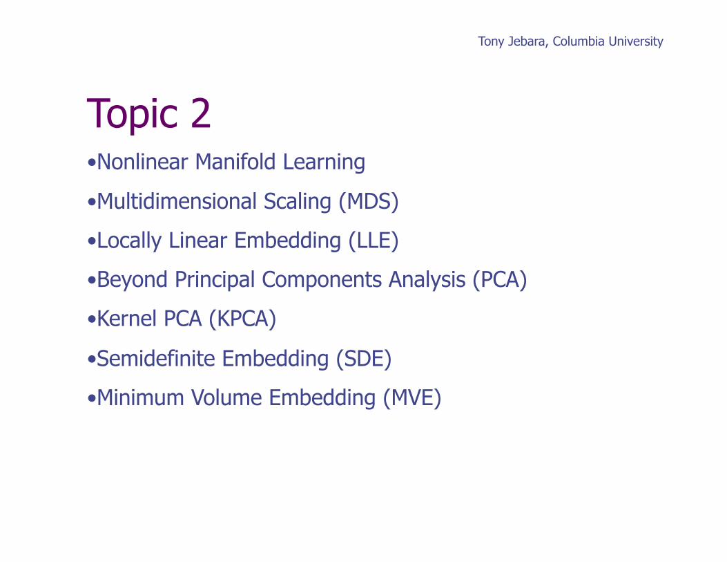
Topic 2 • Nonlinear Manifold Learning
• Multidimensional Scaling (MDS)
• Locally Linear Embedding (LLE)
• Beyond Principal Components Analysis (PCA)
• Kernel PCA (KPCA)
• Semidefinite Embedding (SDE)
• Minimum Volume Embedding (MVE)
Tony Jebara, Columbia University
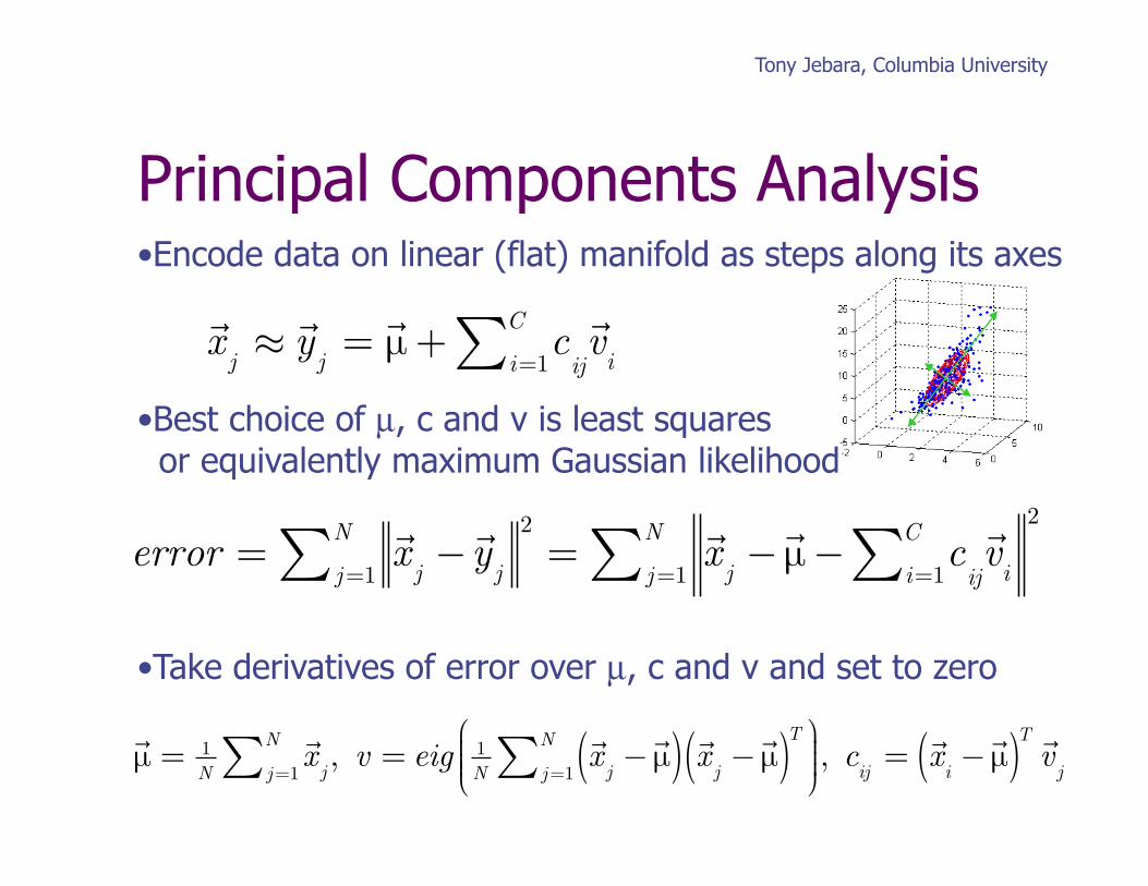
Principal Components Analysis • Encode data on linear (flat) manifold as steps along its axes
• Best choice of µ, c and v is least squares or equivalently maximum Gaussian likelihood
• Take derivatives of error over µ, c and v and set to zero
x
j≈y
j=µ + c
i=1
C∑ ij
v
i
error =
x
j−y
j
2
j =1
N∑ =x
j−µ− c
i=1
C∑ ij
v
i
2
j =1
N∑
µ = 1
N
x
jj =1
N∑ , v = eig 1N
x
j−µ( ) xj
−µ( )Tj =1
N∑⎛⎝⎜⎜⎜
⎞⎠⎟⎟⎟, c
ij=x
i−µ( )T vj
Tony Jebara, Columbia University
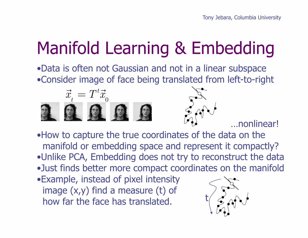
Manifold Learning & Embedding • Data is often not Gaussian and not in a linear subspace • Consider image of face being translated from left-to-right
…nonlinear! • How to capture the true coordinates of the data on the manifold or embedding space and represent it compactly? • Unlike PCA, Embedding does not try to reconstruct the data • Just finds better more compact coordinates on the manifold • Example, instead of pixel intensity image (x,y) find a measure (t) of how far the face has translated.
x
t= Tt x
0
t
Tony Jebara, Columbia University
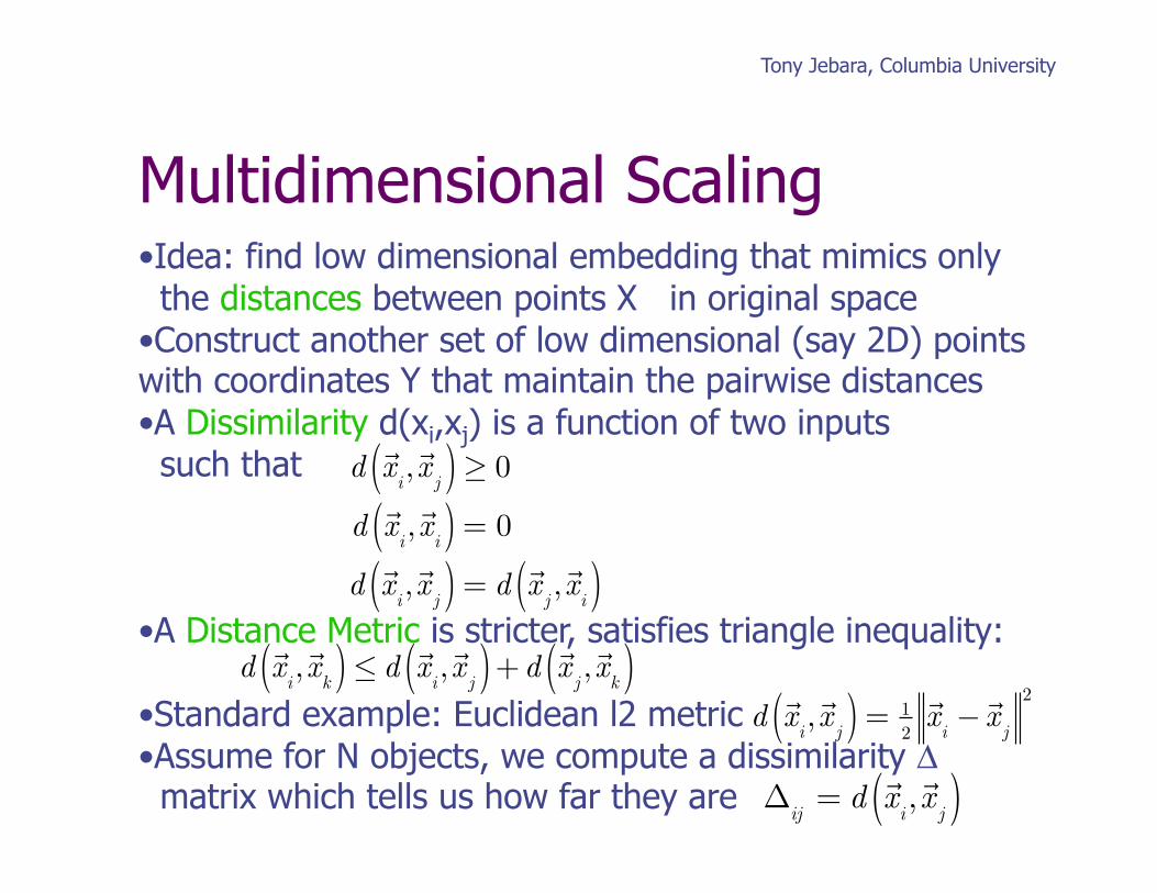
Multidimensional Scaling • Idea: find low dimensional embedding that mimics only the distances between points X in original space • Construct another set of low dimensional (say 2D) points with coordinates Y that maintain the pairwise distances • A Dissimilarity d(xi,xj) is a function of two inputs such that
• A Distance Metric is stricter, satisfies triangle inequality:
• Standard example: Euclidean l2 metric • Assume for N objects, we compute a dissimilarity Δ matrix which tells us how far they are
dx
i,x
j( )≥ 0
dx
i,x
i( ) = 0
dx
i,x
j( ) = dx
j,x
i( )
dx
i,x
k( )≤ dx
i,x
j( ) +dx
j,x
k( ) dx
i,x
j( ) = 12
x
i−x
j
2
Δ
ij= d
x
i,x
j( )
Tony Jebara, Columbia University
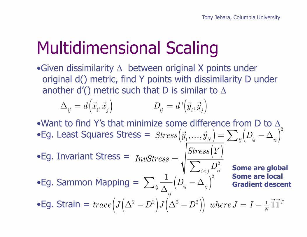
Multidimensional Scaling • Given dissimilarity Δ between original X points under original d() metric, find Y points with dissimilarity D under another d’() metric such that D is similar to Δ
• Want to find Y’s that minimize some difference from D to Δ • Eg. Least Squares Stress =
• Eg. Invariant Stress =
• Eg. Sammon Mapping =
• Eg. Strain =
Δ
ij= d
x
i,x
j( ) Dij
= d 'y
i,y
j( )
Stress
y
1,…,y
N( ) = Dij−Δ
ij( )2
ij∑
InvStress =Stress Y( )
Dij2
i<j∑
1Δ
ij
Dij−Δ
ij( )2
ij∑
trace J Δ2 −D2( )J Δ2 −D2( )( ) whereJ = I − 1
N
11T
Some are global Some are local Gradient descent
Tony Jebara, Columbia University
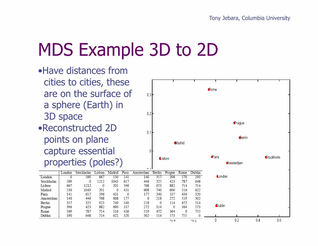
• Have distances from cities to cities, these are on the surface of a sphere (Earth) in 3D space • Reconstructed 2D points on plane capture essential properties (poles?)
MDS Example 3D to 2D
Tony Jebara, Columbia University
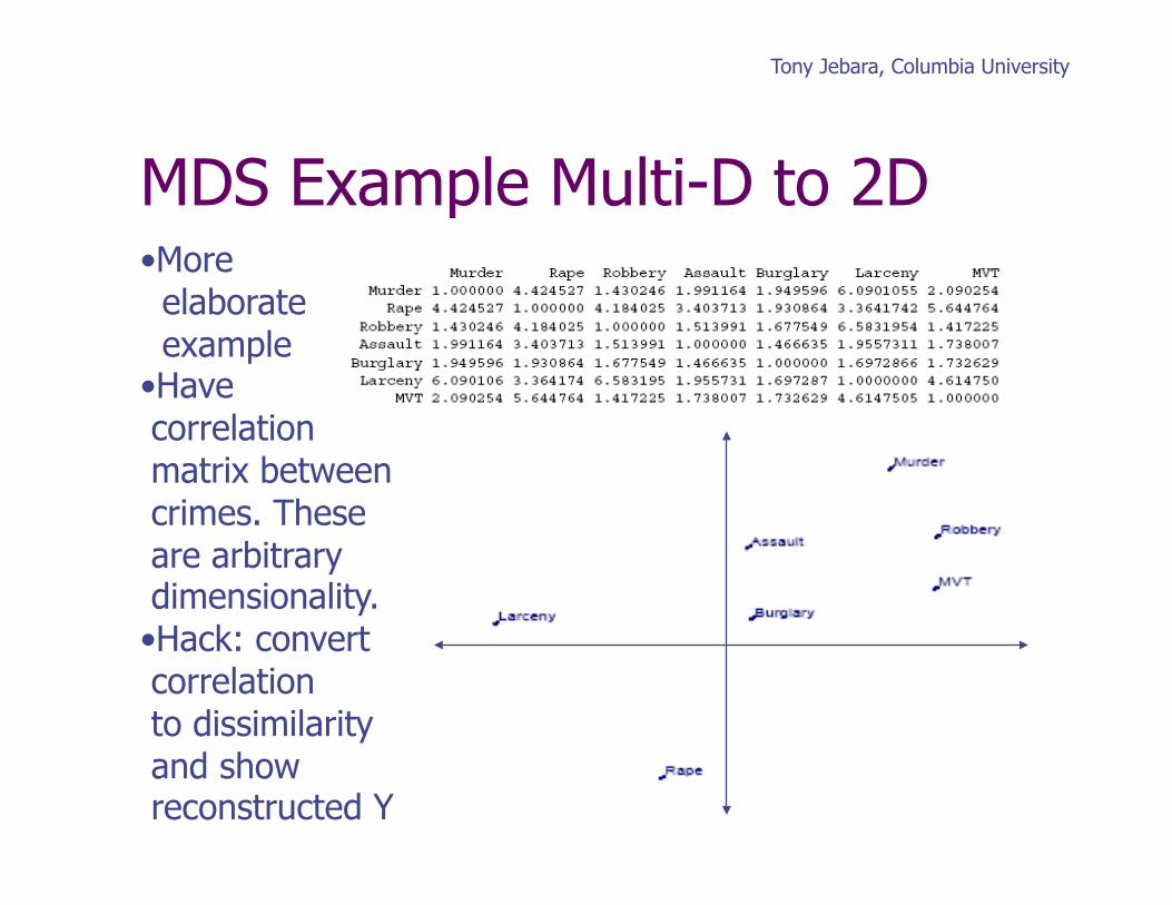
• More elaborate example • Have correlation matrix between crimes. These are arbitrary dimensionality. • Hack: convert correlation to dissimilarity and show reconstructed Y
MDS Example Multi-D to 2D
Tony Jebara, Columbia University
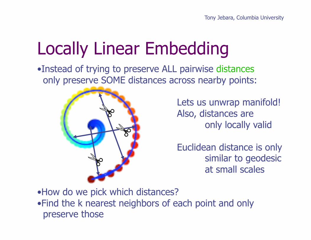
• Instead of trying to preserve ALL pairwise distances only preserve SOME distances across nearby points:
Lets us unwrap manifold! Also, distances are only locally valid
Euclidean distance is only similar to geodesic at small scales
• How do we pick which distances? • Find the k nearest neighbors of each point and only preserve those
Locally Linear Embedding
Tony Jebara, Columbia University
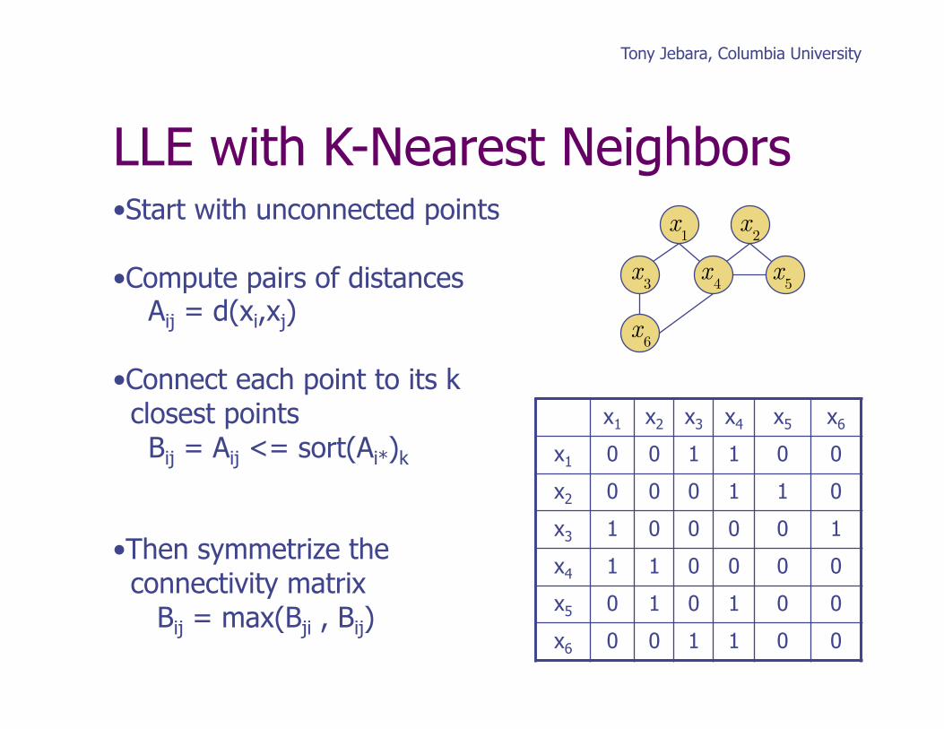
LLE with K-Nearest Neighbors • Start with unconnected points
• Compute pairs of distances Aij = d(xi,xj)
• Connect each point to its k closest points Bij = Aij <= sort(Ai*)k
• Then symmetrize the connectivity matrix Bij = max(Bji , Bij)
x1 x2 x3 x4 x5 x6
x1 0 0 1 1 0 0
x2 0 0 0 1 1 0
x3 1 0 0 0 0 1
x4 1 1 0 0 0 0
x5 0 1 0 1 0 0
x6 0 0 1 1 0 0
x2 x1
x4 x3 x5
x6
Tony Jebara, Columbia University
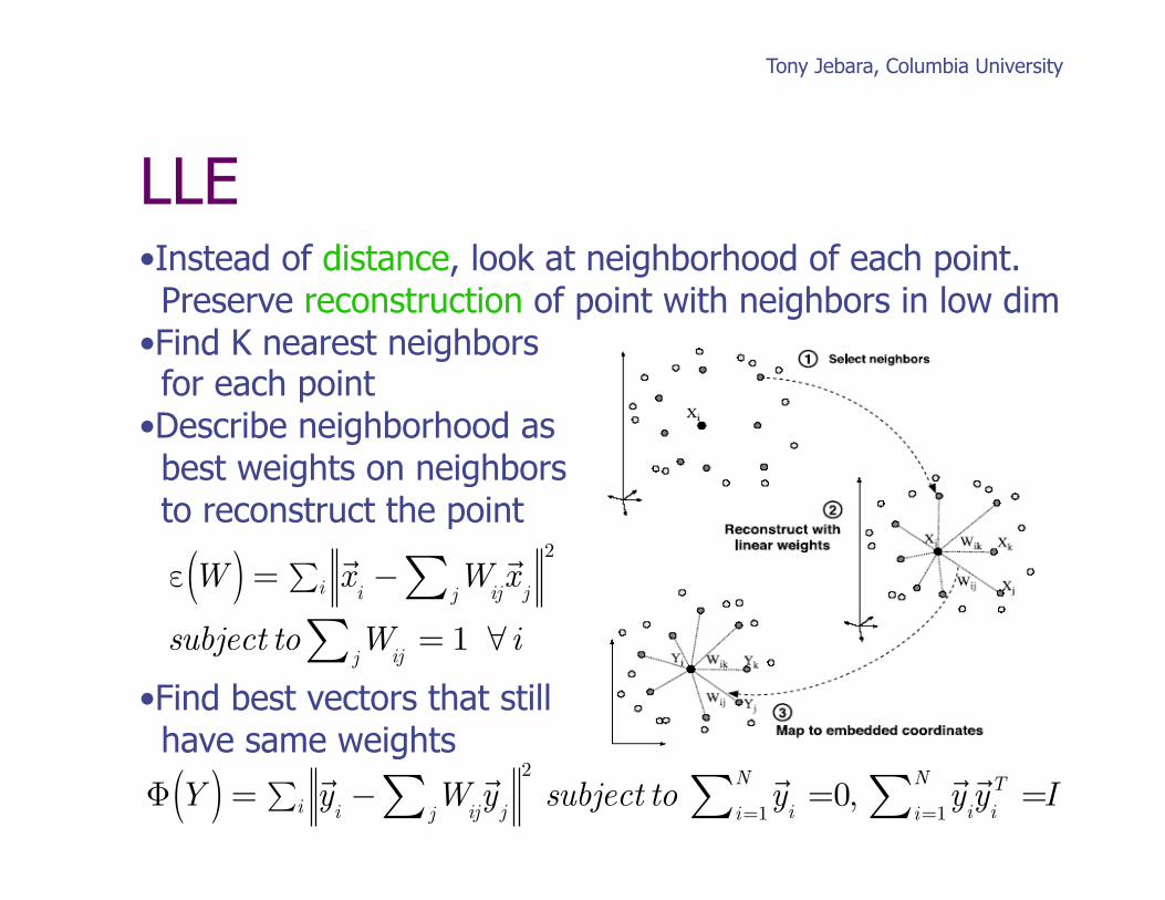
• Instead of distance, look at neighborhood of each point. Preserve reconstruction of point with neighbors in low dim • Find K nearest neighbors for each point • Describe neighborhood as best weights on neighbors to reconstruct the point
• Find best vectors that still have same weights
LLE
εW( ) =x
i− W
ij
x
jj∑2
i∑
subject to Wijj∑ = 1 ∀ i
Φ Y( ) =
y
i− W
ij
y
jj∑2
i∑ subject toy
i=
i=1
N∑ 0,y
i
y
iT =
i=1
N∑ I
Tony Jebara, Columbia University
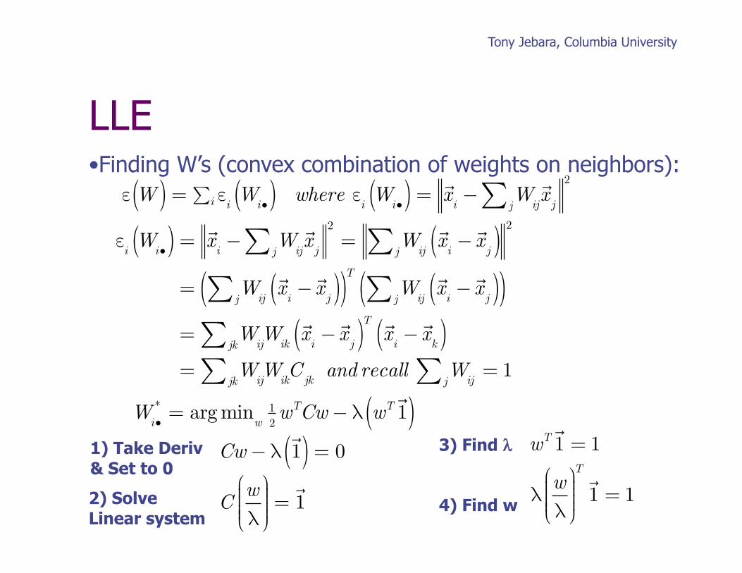
LLE • Finding W’s (convex combination of weights on neighbors):
εW( ) = ε
iW
i•( )i∑ where εiW
i•( ) =x
i− W
ij
x
jj∑2
εiW
i•( ) =x
i− W
ij
x
jj∑2
= Wij
x
i−x
j( )j∑2
= Wij
x
i−x
j( )j∑( )T
Wij
x
i−x
j( )j∑( )= W
ijW
ik
x
i−x
j( )T xi−x
k( )jk∑= W
ijW
ikC
jkjk∑ and recall Wij
= 1j∑
W
i•* = arg min
w12wTCw−λ wT
1( )
Cw−λ1( ) = 0
Cwλ
⎛
⎝⎜⎜⎜⎜
⎞
⎠⎟⎟⎟⎟
=1
1) Take Deriv & Set to 0
2) Solve Linear system
3) Find λ
4) Find w
wT1 = 1
λwλ
⎛
⎝⎜⎜⎜⎜
⎞
⎠⎟⎟⎟⎟
T 1 = 1
Tony Jebara, Columbia University
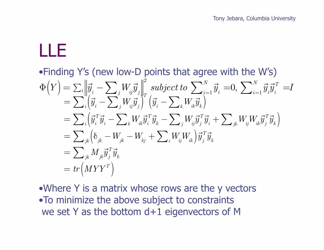
LLE • Finding Y’s (new low-D points that agree with the W’s)
• Where Y is a matrix whose rows are the y vectors • To minimize the above subject to constraints we set Y as the bottom d+1 eigenvectors of M
=y
i− W
ij
y
jj∑( )T yi− W
ik
y
kk∑( )i∑=
y
iT y
i− W
ik
y
iT y
kk∑ − Wij
y
jT y
ij∑ + WijW
ik
y
jT y
kjk∑( )i∑= δ
jk−W
jk−W
kj+ W
ijW
iki∑( ) yjT y
kjk∑= M
jk
y
jT y
kjk∑= tr MYYT( )
Φ Y( ) =
y
i− W
ij
y
jj∑2
i∑ subject toy
i=
i=1
N∑ 0,y
i
y
iT =
i=1
N∑ I
Tony Jebara, Columbia University
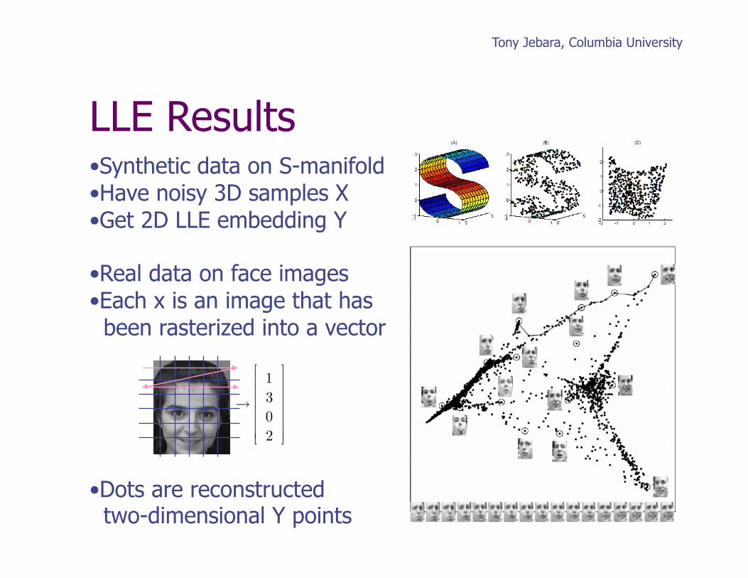
• Synthetic data on S-manifold • Have noisy 3D samples X • Get 2D LLE embedding Y
• Real data on face images • Each x is an image that has been rasterized into a vector
• Dots are reconstructed two-dimensional Y points
LLE Results
→
1302
⎡
⎣
⎢⎢⎢⎢⎢⎢
⎤
⎦
⎥⎥⎥⎥⎥⎥
Tony Jebara, Columbia University
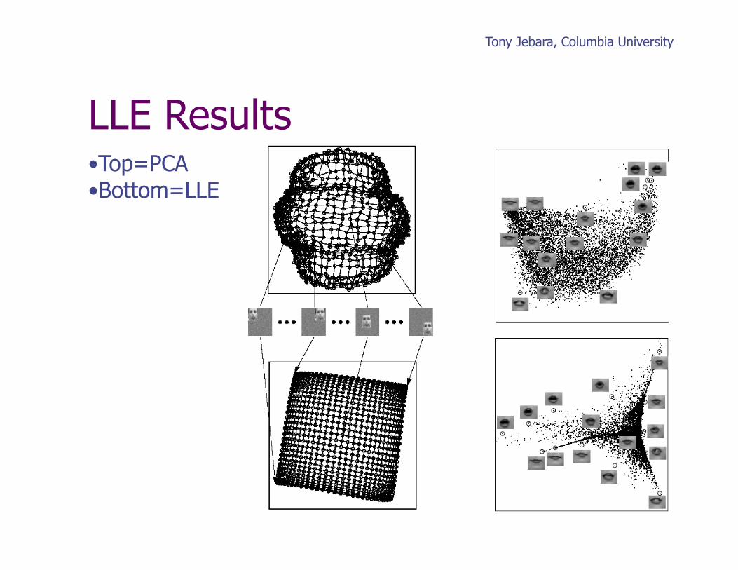
• Top=PCA • Bottom=LLE
LLE Results
Tony Jebara, Columbia University
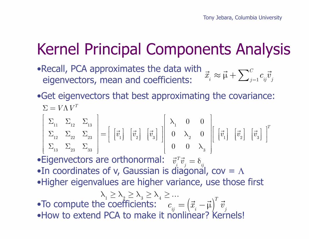
• Recall, PCA approximates the data with eigenvectors, mean and coefficients:
• Get eigenvectors that best approximating the covariance:
• Eigenvectors are orthonormal: • In coordinates of v, Gaussian is diagonal, cov = Λ • Higher eigenvalues are higher variance, use those first
• To compute the coefficients: • How to extend PCA to make it nonlinear? Kernels!
Kernel Principal Components Analysis
x
i≈µ + c
ij
v
jj =1
C∑
Σ =VΛVT
Σ11Σ
12Σ
13
Σ12Σ
22Σ
23
Σ13Σ
23Σ
33
⎡
⎣
⎢⎢⎢⎢⎢⎢
⎤
⎦
⎥⎥⎥⎥⎥⎥
=v
1⎡⎣⎢⎤⎦⎥v
2⎡⎣⎢⎤⎦⎥v
3⎡⎣⎢⎤⎦⎥
⎡⎣⎢
⎤⎦⎥
λ1
0 0
0 λ2
0
0 0 λ3
⎡
⎣
⎢⎢⎢⎢⎢⎢
⎤
⎦
⎥⎥⎥⎥⎥⎥
v
1⎡⎣⎢⎤⎦⎥v
2⎡⎣⎢⎤⎦⎥v
3⎡⎣⎢⎤⎦⎥
⎡⎣⎢
⎤⎦⎥T
c
ij=x
i−µ( )T vj
v
iT v
j= δ
ij
λ1≥ λ
2≥ λ
3≥ λ
4≥…
Tony Jebara, Columbia University
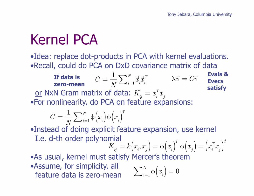
• Idea: replace dot-products in PCA with kernel evaluations. • Recall, could do PCA on DxD covariance matrix of data
or NxN Gram matrix of data: • For nonlinearity, do PCA on feature expansions:
• Instead of doing explicit feature expansion, use kernel I.e. d-th order polynomial
• As usual, kernel must satisfy Mercer’s theorem • Assume, for simplicity, all feature data is zero-mean
Kernel PCA
C =
1N
x
i
x
iT
i=1
N∑
K
ij= x
iTx
j
K
ij= k x
i,x
j( ) = φ xi( )T φ x
j( ) = xiTx
j( )d
C =
1N
φ xi( )φ x
i( )Ti=1
N∑
λv = C
v
Evals & Evecs satisfy
φ x
i( ) = 0i=1
N∑
If data is zero-mean
Tony Jebara, Columbia University
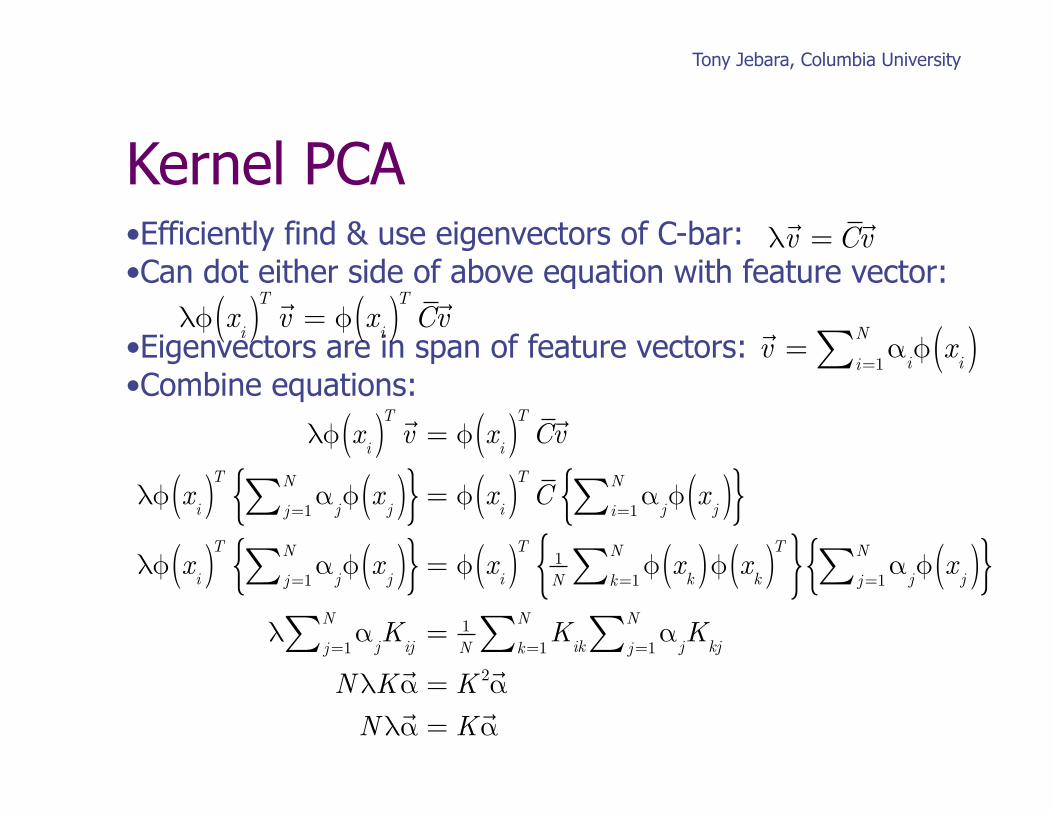
Kernel PCA • Efficiently find & use eigenvectors of C-bar: • Can dot either side of above equation with feature vector:
• Eigenvectors are in span of feature vectors: • Combine equations:
λv = C
v
v = α
iφ x
i( )i=1
N∑ λφ x
i( )T v = φ xi( )T C
v
λφ xi( )T v = φ x
i( )T Cv
λφ xi( )T α
jφ x
j( )j =1
N∑{ } = φ xi( )T C α
jφ x
j( )i=1
N∑{ }λφ x
i( )T αjφ x
j( )j =1
N∑{ } = φ xi( )T 1
Nφ x
k( )φ xk( )Tk=1
N∑{ } αjφ x
j( )j =1
N∑{ }λ α
jK
ijj =1
N∑ = 1N
Kikk=1
N∑ αjK
kjj =1
N∑NλK
α = K 2 α
Nλα = K
α
Tony Jebara, Columbia University
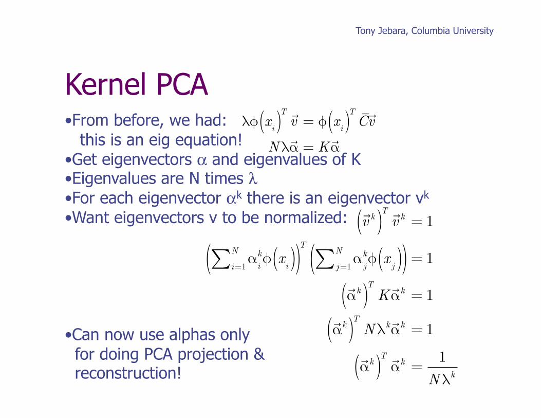
• From before, we had: this is an eig equation! • Get eigenvectors α and eigenvalues of K • Eigenvalues are N times λ • For each eigenvector αk there is an eigenvector vk • Want eigenvectors v to be normalized:
• Can now use alphas only for doing PCA projection & reconstruction!
Kernel PCA
λφ xi( )T v = φ x
i( )T Cv
Nλα = K
α
v k( )T v k = 1
αikφ x
i( )i=1
N∑( )T
αjkφ x
j( )j =1
N∑( ) = 1
αk( )T K
αk = 1
αk( )T Nλk αk = 1
αk( )T αk =
1Nλk
Tony Jebara, Columbia University
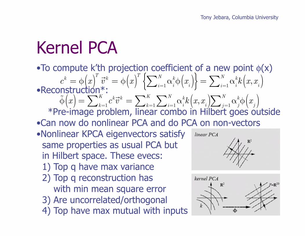
Kernel PCA • To compute k’th projection coefficient of a new point φ(x)
• Reconstruction*:
*Pre-image problem, linear combo in Hilbert goes outside • Can now do nonlinear PCA and do PCA on non-vectors • Nonlinear KPCA eigenvectors satisfy same properties as usual PCA but in Hilbert space. These evecs: 1) Top q have max variance 2) Top q reconstruction has with min mean square error 3) Are uncorrelated/orthogonal 4) Top have max mutual with inputs
ck = φ x( )T v k = φ x( )T α
ikφ x
i( )i=1
N∑{ } = αikk x,x
i( )i=1
N∑
φ x( ) = ck
k=1
K∑ v k = α
ikk x,x
i( )i=1
N∑ αjkφ x
j( )j =1
N∑k=1
K∑
Tony Jebara, Columbia University
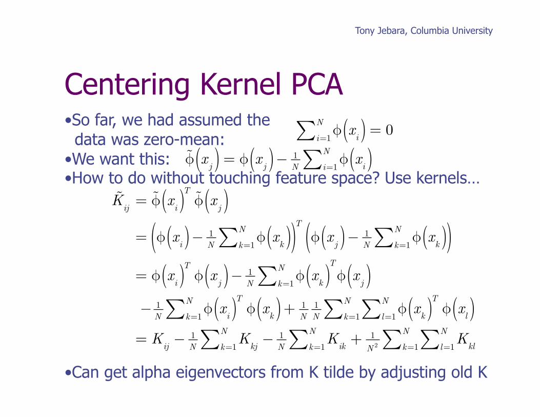
Centering Kernel PCA • So far, we had assumed the data was zero-mean: • We want this: • How to do without touching feature space? Use kernels…
• Can get alpha eigenvectors from K tilde by adjusting old K
φ x
i( ) = 0i=1
N∑
φ x
j( ) = φ xj( )− 1
Nφ x
i( )i=1
N∑
Kij
= φ xi( )T φ x
j( )= φ x
i( )− 1N
φ xk( )k=1
N∑( )T
φ xj( )− 1
Nφ x
k( )k=1
N∑( )= φ x
i( )T φ xj( )− 1
Nφ x
k( )k=1
N∑T
φ xj( )
− 1N
φ xi( )T φ x
k( )k=1
N∑ + 1N
1N
φ xk( )T φ x
l( )l=1
N∑k=1
N∑= K
ij− 1
NK
kjk=1
N∑ − 1N
Kikk=1
N∑ + 1N 2
Kkll=1
N∑k=1
N∑
Tony Jebara, Columbia University
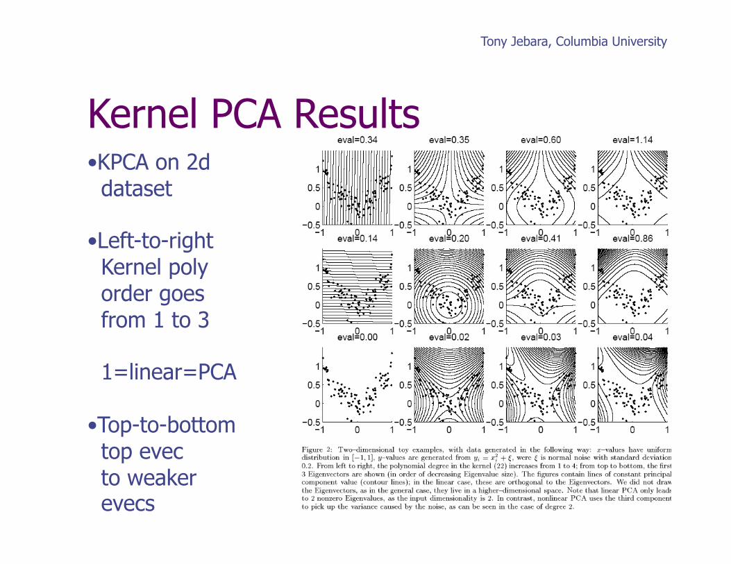
• KPCA on 2d dataset
• Left-to-right Kernel poly order goes from 1 to 3
1=linear=PCA
• Top-to-bottom top evec to weaker evecs
Kernel PCA Results
Tony Jebara, Columbia University
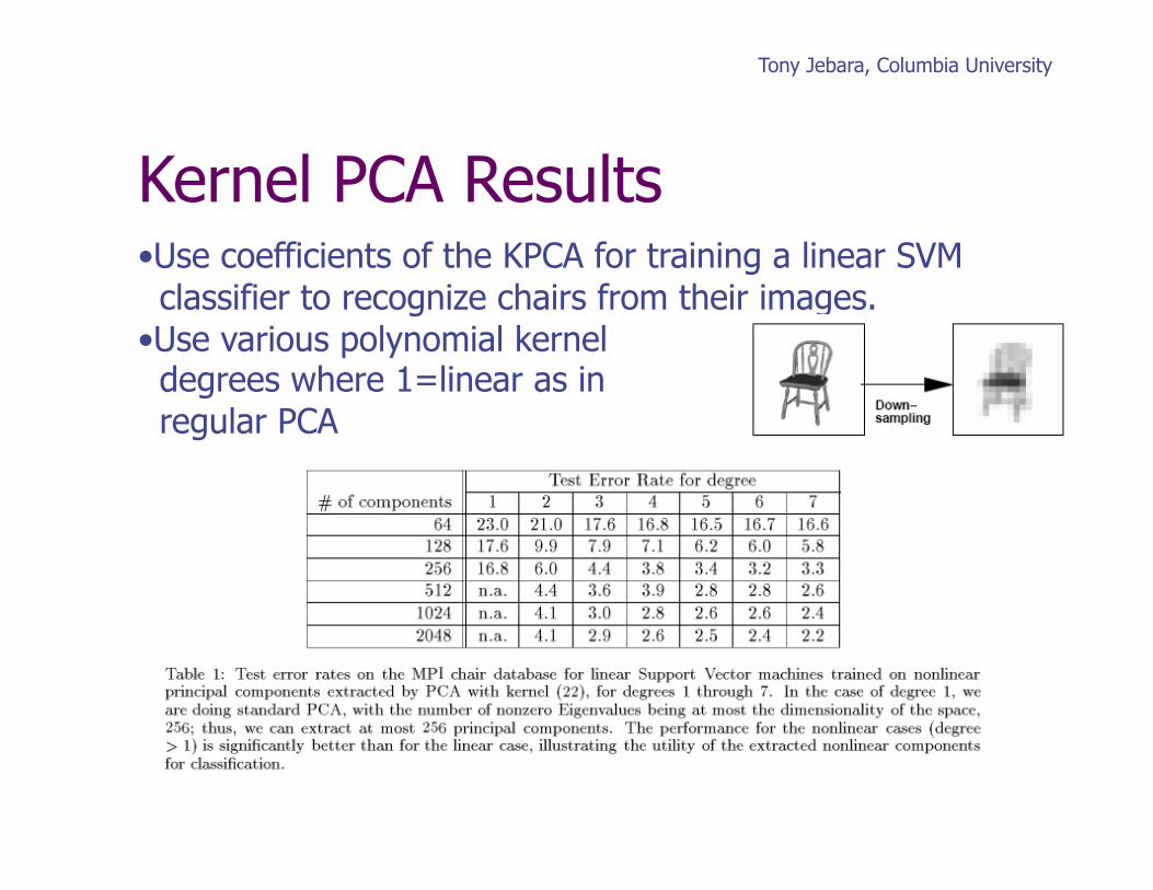
• Use coefficients of the KPCA for training a linear SVM classifier to recognize chairs from their images. • Use various polynomial kernel degrees where 1=linear as in regular PCA
Kernel PCA Results
Tony Jebara, Columbia University
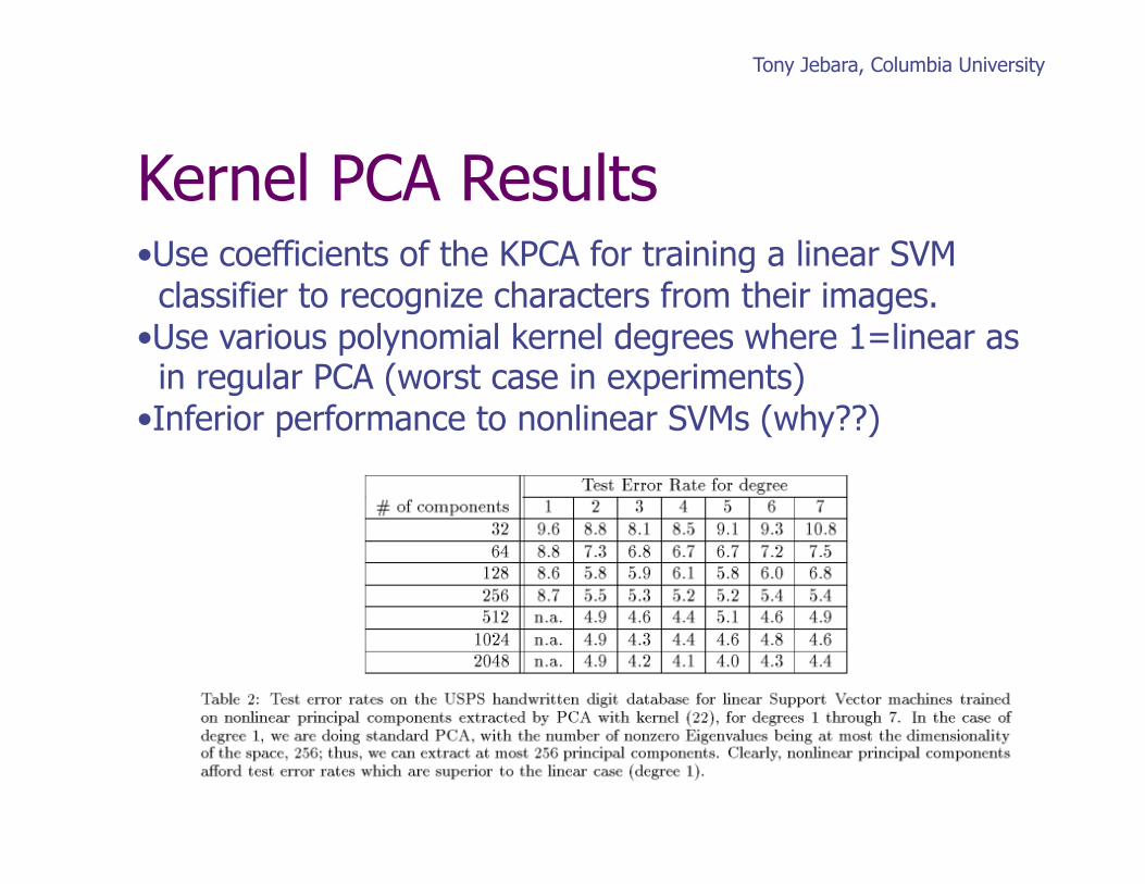
• Use coefficients of the KPCA for training a linear SVM classifier to recognize characters from their images. • Use various polynomial kernel degrees where 1=linear as in regular PCA (worst case in experiments) • Inferior performance to nonlinear SVMs (why??)
Kernel PCA Results
Tony Jebara, Columbia University
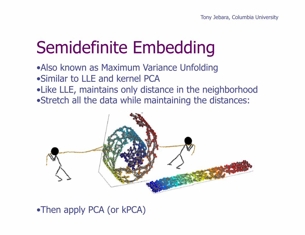
• Also known as Maximum Variance Unfolding • Similar to LLE and kernel PCA • Like LLE, maintains only distance in the neighborhood • Stretch all the data while maintaining the distances:
• Then apply PCA (or kPCA)
Semidefinite Embedding
Tony Jebara, Columbia University
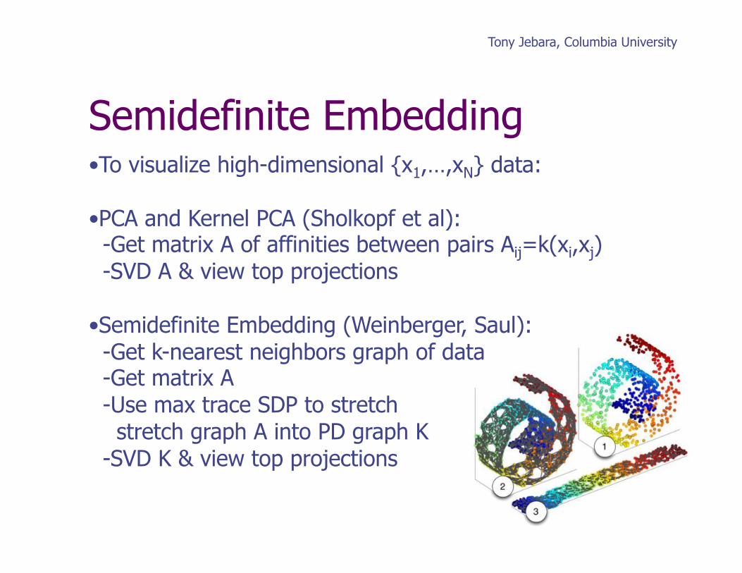
• To visualize high-dimensional {x1,…,xN} data:
• PCA and Kernel PCA (Sholkopf et al): -Get matrix A of affinities between pairs Aij=k(xi,xj) -SVD A & view top projections
• Semidefinite Embedding (Weinberger, Saul): -Get k-nearest neighbors graph of data -Get matrix A -Use max trace SDP to stretch stretch graph A into PD graph K -SVD K & view top projections
Semidefinite Embedding
Tony Jebara, Columbia University
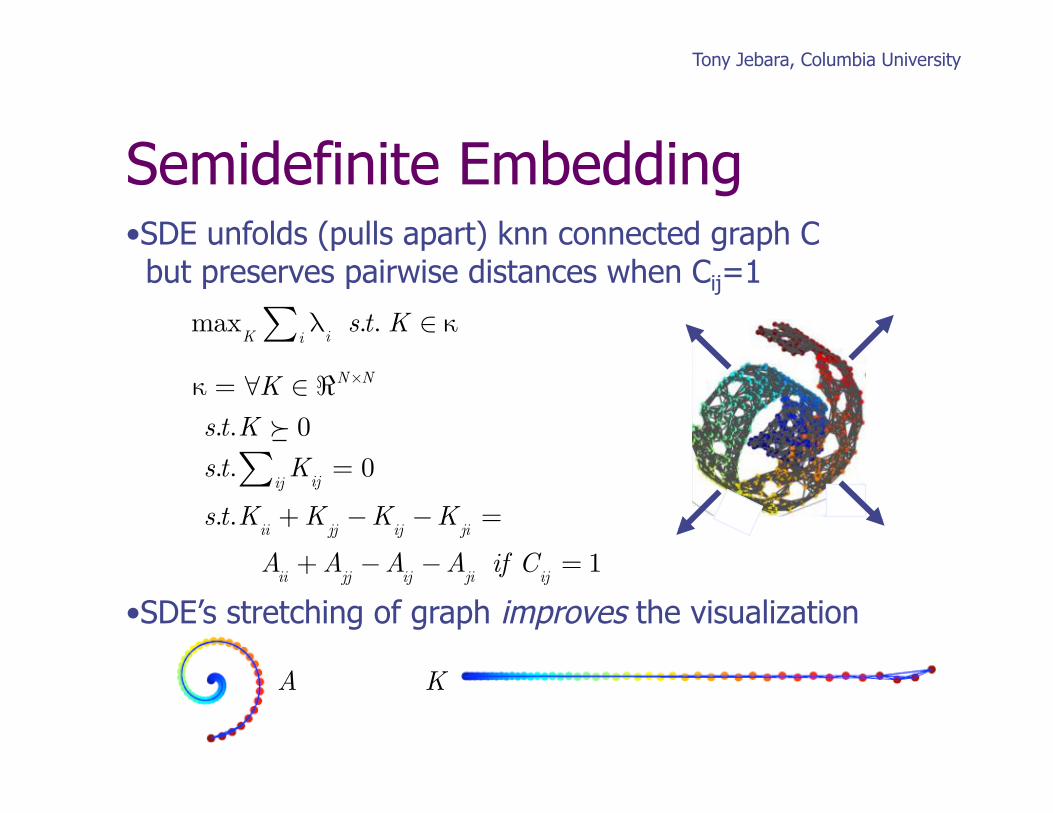
• SDE unfolds (pulls apart) knn connected graph C but preserves pairwise distances when Cij=1
• SDE’s stretching of graph improves the visualization
Semidefinite Embedding
max
Kλ
ii∑ s.t. K ∈ κ
κ = ∀K ∈ ℜN×N
s.t.K 0s.t. K
ij= 0
ij∑s.t.K
ii+ K
jj−K
ij−K
ji=
Aii
+ Ajj−A
ij−A
jiif C
ij= 1
Tony Jebara, Columbia University
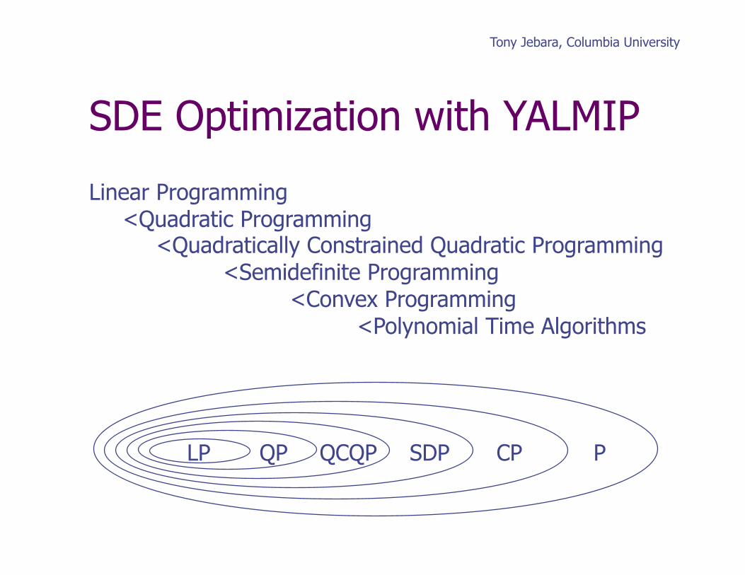
Linear Programming <Quadratic Programming <Quadratically Constrained Quadratic Programming <Semidefinite Programming <Convex Programming <Polynomial Time Algorithms
SDE Optimization with YALMIP
P CP SDP QCQP QP LP
Tony Jebara, Columbia University
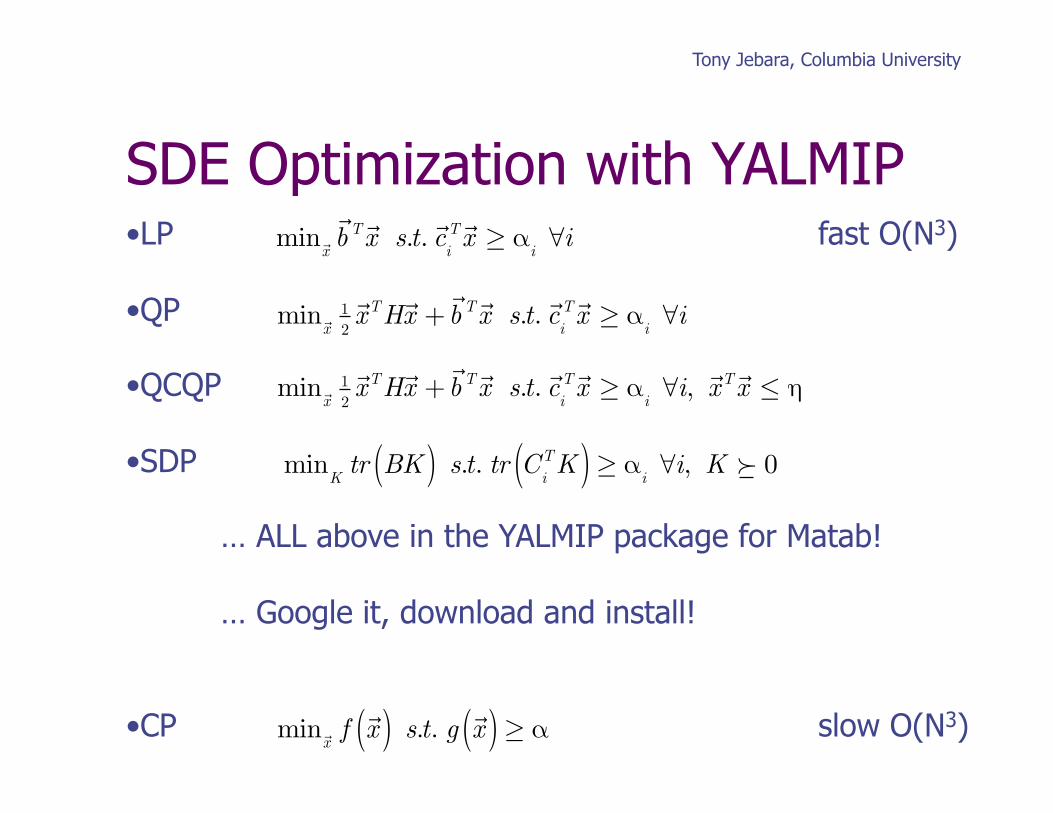
• LP fast O(N3) • QP
• QCQP
• SDP
… ALL above in the YALMIP package for Matab!
… Google it, download and install! • CP slow O(N3)
SDE Optimization with YALMIP min
x
bT x s.t.
c
iT x ≥ α
i∀i
min x
12
xTHx +bT x s.t.
c
iT x ≥ α
i∀i
min x
12
xTHx +bT x s.t.
c
iT x ≥ α
i∀i,xT x ≤ η
min
Ktr BK( ) s.t. tr C
iTK( )≥ αi
∀i, K 0
min
xfx( ) s.t. g
x( )≥ α
Tony Jebara, Columbia University
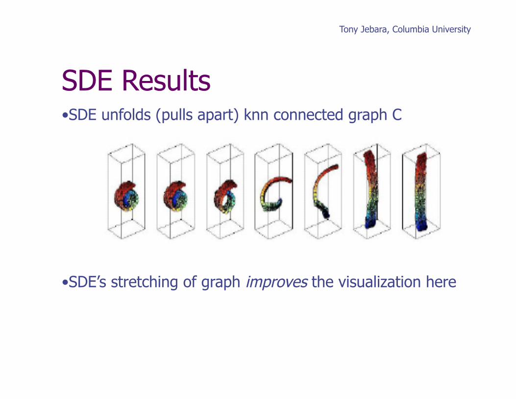
• SDE unfolds (pulls apart) knn connected graph C
• SDE’s stretching of graph improves the visualization here
SDE Results
Tony Jebara, Columbia University
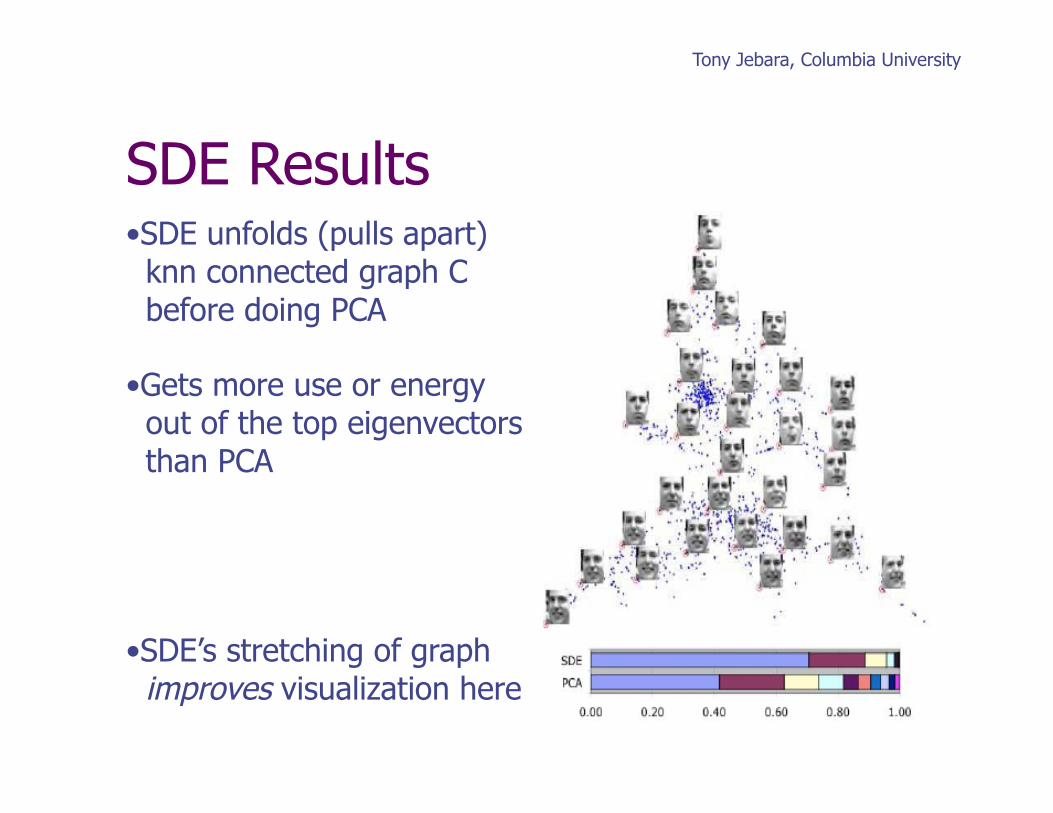
• SDE unfolds (pulls apart) knn connected graph C before doing PCA
• Gets more use or energy out of the top eigenvectors than PCA
• SDE’s stretching of graph improves visualization here
SDE Results
Tony Jebara, Columbia University
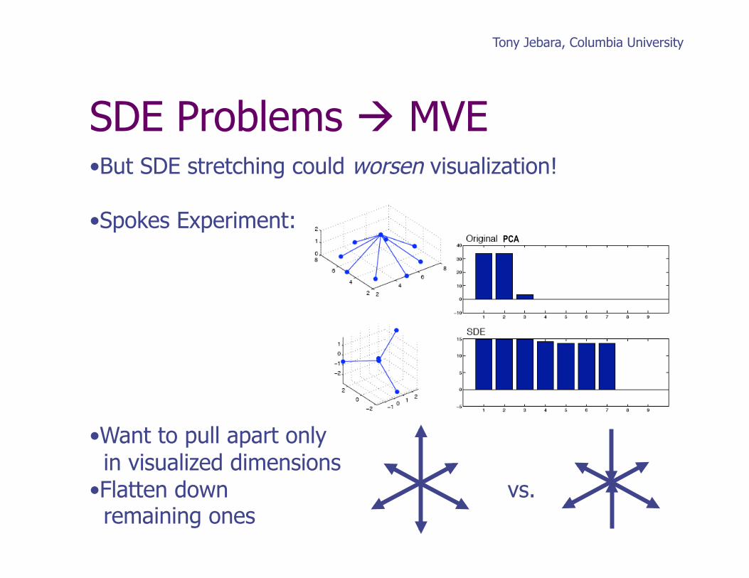
SDE Problems MVE • But SDE stretching could worsen visualization!
• Spokes Experiment:
• Want to pull apart only in visualized dimensions • Flatten down vs. remaining ones
PCA
Tony Jebara
33
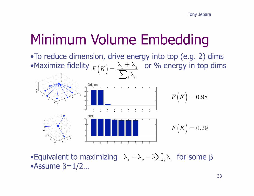
• To reduce dimension, drive energy into top (e.g. 2) dims • Maximize fidelity or % energy in top dims
• Equivalent to maximizing for some β • Assume β=1/2…
Minimum Volume Embedding
F K( ) =
λ1
+ λ2
λii∑
F K( ) = 0.98
F K( ) = 0.29
λ
1+ λ
2−β λ
ii∑
Tony Jebara, Columbia University
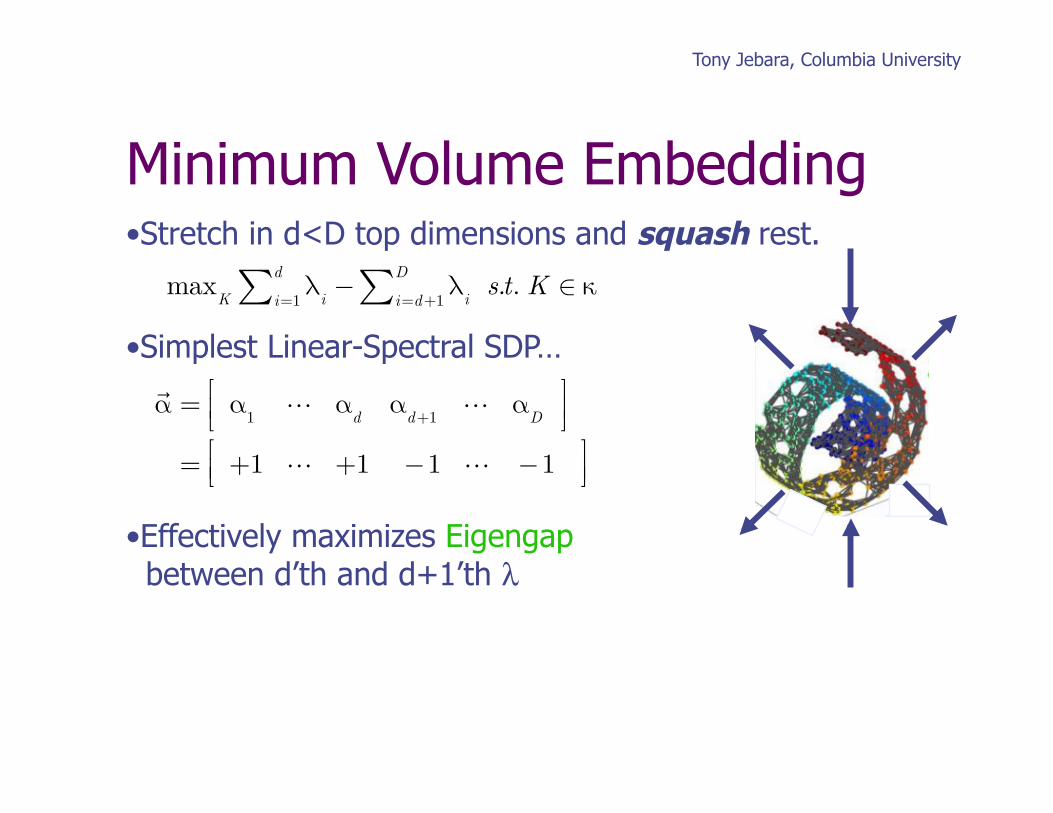
• Stretch in d<D top dimensions and squash rest.
• Simplest Linear-Spectral SDP…
• Effectively maximizes Eigengap between d’th and d+1’th λ
Minimum Volume Embedding
max
Kλ
ii=1
d∑ − λii=d+1
D∑ s.t. K ∈ κ
α = α
1 α
dα
d+1 α
D⎡⎣⎢
⎤⎦⎥
= +1 +1 −1 −1⎡⎣⎢
⎤⎦⎥
Tony Jebara, Columbia University
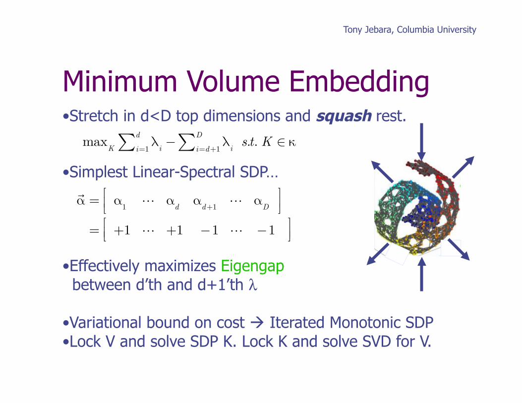
• Stretch in d<D top dimensions and squash rest.
• Simplest Linear-Spectral SDP…
• Effectively maximizes Eigengap between d’th and d+1’th λ
• Variational bound on cost Iterated Monotonic SDP • Lock V and solve SDP K. Lock K and solve SVD for V.
Minimum Volume Embedding
max
Kλ
ii=1
d∑ − λii=d+1
D∑ s.t. K ∈ κ
α = α
1 α
dα
d+1 α
D⎡⎣⎢
⎤⎦⎥
= +1 +1 −1 −1⎡⎣⎢
⎤⎦⎥
Tony Jebara, Columbia University
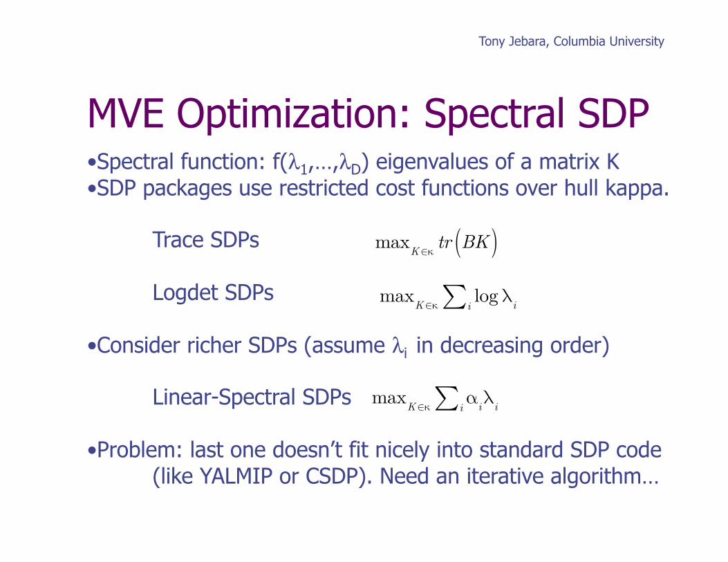
• Spectral function: f(λ1,…,λD) eigenvalues of a matrix K • SDP packages use restricted cost functions over hull kappa. Trace SDPs
Logdet SDPs
• Consider richer SDPs (assume λi in decreasing order)
Linear-Spectral SDPs
• Problem: last one doesn’t fit nicely into standard SDP code (like YALMIP or CSDP). Need an iterative algorithm…
MVE Optimization: Spectral SDP
max
K∈κtr BK( )
max
K∈κlogλ
ii∑
max
K∈κα
iλ
ii∑
Tony Jebara, Columbia University
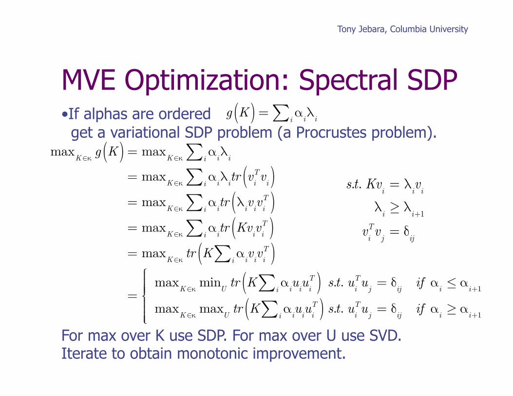
• If alphas are ordered get a variational SDP problem (a Procrustes problem).
For max over K use SDP. For max over U use SVD. Iterate to obtain monotonic improvement.
MVE Optimization: Spectral SDP g K( ) = α
iλ
ii∑
maxK∈κ
g K( ) = maxK∈κ
αiλ
ii∑= max
K∈κα
iλ
itr v
iTv
i( )i∑= max
K∈κα
itr λ
iv
iv
iT( )i∑
= maxK∈κ
αitr Kv
iv
iT( )i∑
= maxK∈κ
tr K αiv
iv
iT
i∑( )
=max
K∈κmin
Utr K α
iu
iu
iT
i∑( ) s.t. uiTu
j= δ
ijif α
i≤ α
i+1
maxK∈κ
maxU
tr K αiu
iu
iT
i∑( ) s.t. uiTu
j= δ
ijif α
i≥ α
i+1
⎧
⎨
⎪⎪⎪⎪
⎩⎪⎪⎪⎪
s.t. Kvi
= λiv
i
λi≥ λ
i+1
viTv
j= δ
ij
Tony Jebara, Columbia University
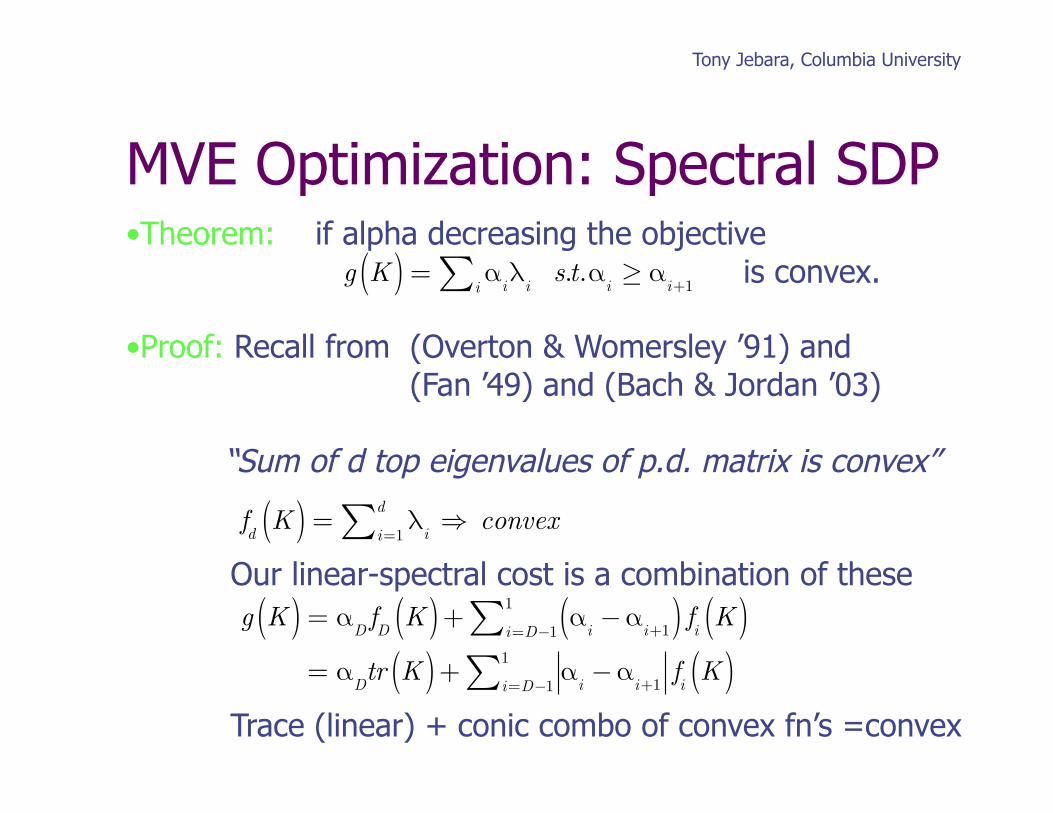
• Theorem: if alpha decreasing the objective
is convex.
• Proof: Recall from (Overton & Womersley ’91) and (Fan ’49) and (Bach & Jordan ’03)
“Sum of d top eigenvalues of p.d. matrix is convex”
Our linear-spectral cost is a combination of these
Trace (linear) + conic combo of convex fn’s =convex
MVE Optimization: Spectral SDP
fd
K( ) = λii=1
d∑ ⇒ convex
g K( ) = α
iλ
ii∑ s.t.αi≥ α
i+1
g K( ) = αDfD
K( ) + αi−α
i+1( ) fi
K( )i=D−1
1∑= α
Dtr K( ) + α
i−α
i+1fi
K( )i=D−1
1∑
Tony Jebara, Columbia University
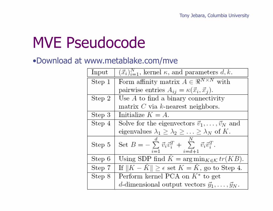
MVE Pseudocode • Download at www.metablake.com/mve
Tony Jebara, Columbia University
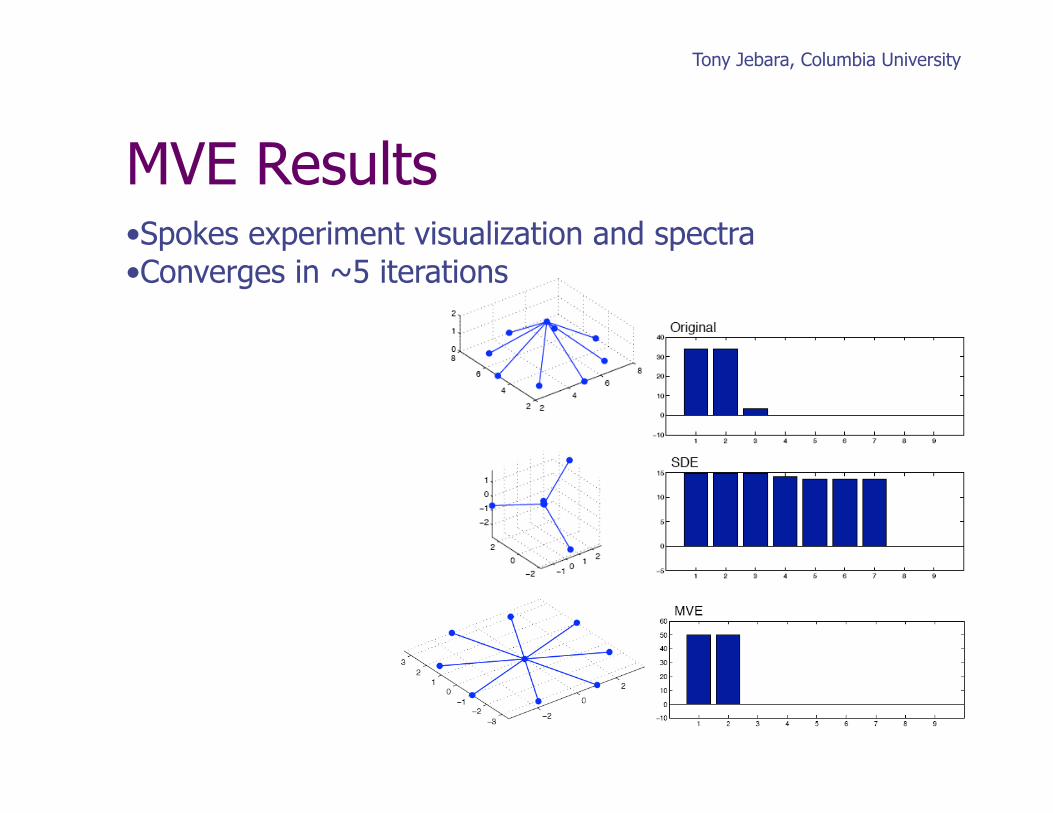
MVE Results • Spokes experiment visualization and spectra • Converges in ~5 iterations

Tony Jebara, Columbia University
MVE Results
PCA
SDE
MVE
• Swissroll Visualization (Connectivity via knn) (d is set to 2)
• Same convergence under random initialization or K=A…
Tony Jebara
42
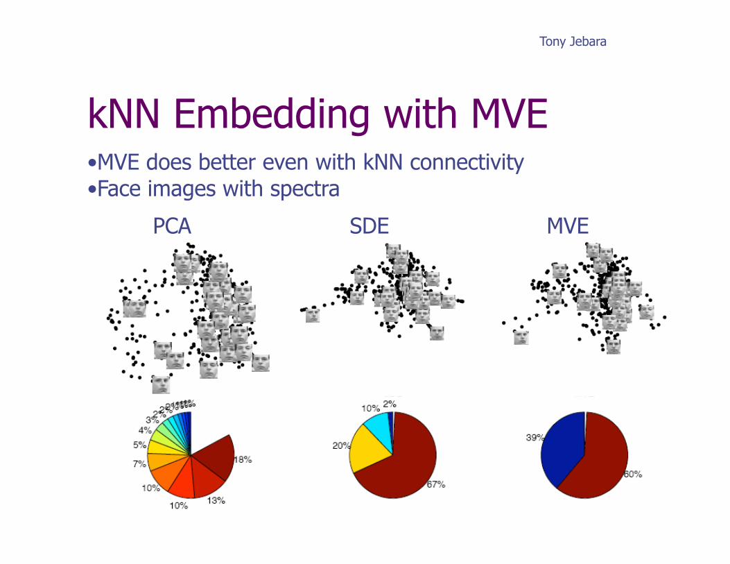
kNN Embedding with MVE • MVE does better even with kNN connectivity • Face images with spectra
PCA SDE MVE
Tony Jebara
43
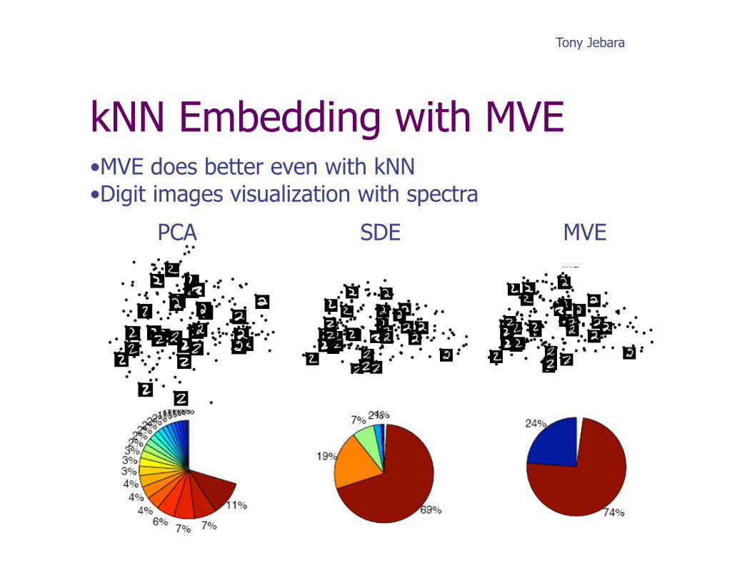
kNN Embedding with MVE • MVE does better even with kNN • Digit images visualization with spectra
PCA SDE MVE
Tony Jebara
44
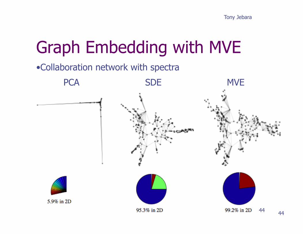
Graph Embedding with MVE • Collaboration network with spectra
PCA SDE MVE
44
Tony Jebara, Columbia University
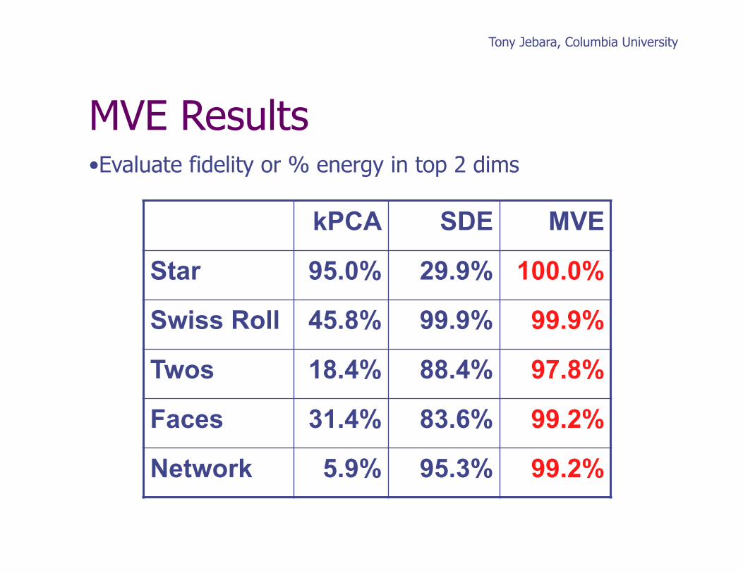
MVE Results
kPCA SDE MVE
Star 95.0% 29.9% 100.0%
Swiss Roll 45.8% 99.9% 99.9%
Twos 18.4% 88.4% 97.8%
Faces 31.4% 83.6% 99.2%
Network 5.9% 95.3% 99.2%
• Evaluate fidelity or % energy in top 2 dims
Tony Jebara, Columbia University
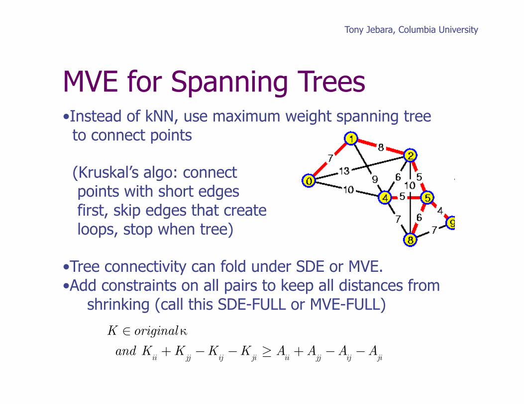
MVE for Spanning Trees • Instead of kNN, use maximum weight spanning tree to connect points
(Kruskal’s algo: connect points with short edges first, skip edges that create loops, stop when tree)
• Tree connectivity can fold under SDE or MVE. • Add constraints on all pairs to keep all distances from shrinking (call this SDE-FULL or MVE-FULL)
K ∈ original κand K
ii+ K
jj−K
ij−K
ji≥ A
ii+ A
jj−A
ij−A
ji
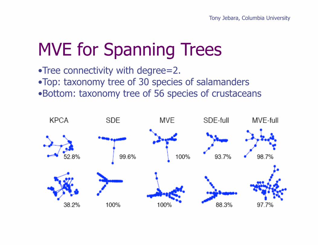
Tony Jebara, Columbia University
MVE for Spanning Trees • Tree connectivity with degree=2. • Top: taxonomy tree of 30 species of salamanders • Bottom: taxonomy tree of 56 species of crustaceans