Susceptibility effects in MRI and 1H MRS

The spurious echo artifact and susceptibility measurements

Åsa Carlsson

Department of Radiation Physics, University of Gothenburg Gothenburg, Sweden, 2009

i

Doctoral Thesis, 2009 Department of Radiation Physics University of Gothenburg Sahlgrenska University Hospital SE-413 45 Gothenburg Sweden Copyright © Åsa Carlsson ISBN 978-91-628-7688-3 Printed in Sweden by Chalmers Reproservice, Göteborg, 2009 E-publication: http://hdl.handle.net/2077/19002

ii

“Nobody climbs mountains for scientific reasons.  Science is used to raise money for the expeditions,  

but you really climb for the hell of it.”  

Sir Edmund Hillary, one of the first men to climb the Mount Everest

iii

 

iv

Abstract When performing magnetic resonance (MR) experiments, a strong homogeneous magnetic field is often preferred, especially in clinical applications. However, all objects that are placed in the magnetic field will disturb the field homogeneity and cause local magnetic field gradients. In the human body, which consists of a large number of tissues and organs of different shape and susceptibility (the ability to become magnetised), the field distribution becomes very complex. To minimise magnetic field inhomogeneities in the studied region, shim gradients, of linear or higher order, are locally optimised for each measurement.

In clinical MR the trend is towards higher field strengths, from 1.5 T to 3 T and beyond, and this leads to increased susceptibility effects, both in MR imaging (MRI) and MR spectroscopy (MRS). To have control of the susceptibility effects, and achieve high accuracy in phantom studies, it is valuable to have an easy and accessible method for measuring the susceptibility value of the phantom materials. A method which utilises MRI for susceptibility measurements was significantly improved by using an echo planar imaging sequence instead of the standard implementation of a spin echo sequence. An increased sensitivity and accuracy provides a possibility to detect smaller susceptibility differences, to be more flexible in choice of reference liquid or to decrease the sample volume. An automated evaluation method based on model fitting was also developed and this increased the accuracy even further. Finally, the volume susceptibility of two plastics, commonly used in phantoms, was determined.

For small volume 1H MRS in susceptibility influenced regions, the spurious echo artifact has become a problem. It is, however, seldom recognised as a susceptibility artifact. In this thesis a k-space description was introduced and the causes and conditions of this artifact were studied. When the shim gradients are optimised for a small volume, the possibility of achieving a good local shim, i.e. a locally homogenous magnetic field, is increased. An imaging technique was developed, the WSI-scan (water suppression imaging), which visualises how the global effects of the locally optimised shim might shift the water resonance in some regions outside the water suppression bandwidth. When regions of unsuppressed water overlap with the excitation regions of the volume selection, the probability of a spurious echo artifact increases significantly.

To destroy any outer volume signal strong spoiling gradients are implemented in the volume selection sequences. By using the new modified k-space concept it was possible to demonstrate all magnetic configurations and their relative positions prior to acquisition in one single k-space map. This tool showed to be powerful not only for describing the artifact formation but also for evaluating the effective spoiling of unwanted magnetic configurations and it was applied to two volume selection methods, PRESS (point resolved spectroscopy) and STEAM (stimulated echo acquisition mode). The k-space description was verified by in vitro experiments where the magnetic configurations of PRESS were separately refocused into spurious echo artifacts.

This thesis shows that shim gradients are not only likely to shift water resonances of the brain outside the water suppression band, they might also refocus unwanted, and spoiled, magnetic configurations into a spurious echo. The k-space concept, the WSI-scan and the susceptibility measurements all provide important tools for evaluating strategies and prerequisites for high quality 1H MRS of small volumes. Keywords: MRI, 1H MRS, susceptibility, spurious echo, artifact, artefact

v

vi

List of Papers This thesis is based on four papers, which in the text will be referred to by their Roman numerals. I k-space analysis of point resolved spectroscopy (PRESS) with regard to spurious

echoes in in vivo 1H MRS. Göran Starck, Åsa Carlsson, Maria Ljungberg, Eva Forssell-Aronsson NMR in Biomedicine 22(2) (2009) In press

II k-space analysis of the spurious echo artifact in 1H MRS: experimental

verification using PRESS and analysis of the spoiling characteristics in STEAM Åsa Carlsson, Göran Starck, Maria Ljungberg, Eva Forssell-Aronsson

Manuscript III Degraded water suppression in small volume 1H MRS due to shimming

Åsa Carlsson, Maria Ljungberg, Göran Starck, Eva Forssell-Aronsson Submitted 2009

IV Accurate and sensitive measurements of magnetic susceptibility using echo

planar imaging Åsa Carlsson, Göran Starck, Maria Ljungberg, Sven Ekholm, Eva Forssell-Aronsson

Magnetic Resonance Imaging 24 (2006) 1179–1185 Paper I was, with permission from Wiley-Blackwell, reprinted from NMR in Biomedicine, Copyright © (2008) John Wiley & Sons, Ltd. Paper IV was, with permission from Elsevier paper IV, reprinted from Magnetic Resonance Imaging, 24, Pages 1179-85, Copyright © (2006) Elsevier.

vii

Preliminary and Related Reports I Sensitive measurements of magnetic susceptibility in plastics using EPI

Carlsson Å, Starck G, Ljungberg M, Ekholm S, Forssell-Aronsson E European Society for Magnetic Resonance in Medicine and Biology ´19 2002, Cannes, #496

II Bestämning av magnetisk susceptibilitet i plaster med hjälp av MRI.

Carlsson Å, Starck G, Ljungberg M, Ekholm S, Forssell-Aronsson E Svenska Läkaresällskapets riksstämma 2002, Göteborg, MRA 6P

III Sensitive and accurate magnetic susceptibility measurements, a comparison between MRI and MRS Carlsson Å, Starck G, Ljungberg M, Ekholm S, Forssell-Aronsson E European Society for Magnetic Resonance in Medicine and Biology ´21 2004, Copenhagen, #438

IV A phantom design that minimizes the magnetic field inhomogeneity Ljungberg M, Bengtsson F, Carlsson Å, Lagerstrand K, Starck G, Vikhoff-Baaz B, Forssell-Aronsson E. European Society for Magnetic Resonance in Medicine and Biology ’22 2005, Basel, #503

IV The spurious echo artifact in 1H MRS and PRESS Carlsson Å, Ljungberg M, Starck G, Forssell-Aronsson E

International Society for Magnetic Resonance in Medicine ’16 2008, Toronto, #1551

viii

Abbreviations 1H hydrogen αn RF-pulse n (n ∈{1, 2, 3}), e.g. α1

(suffix indicating associated excitation region, magnetisation and signal) αnαm pair of RF-pulses n and m (n, m ∈{1, 2, 3}), e.g. α1α3

(suffix indicating associated excitation region, magnetisation and signal) α1α2α3 all three RF-pulses of the volume selection sequence

(suffix indicating associated excitation region, magnetisation and signal) B0 the external field of an MR-system [T] CHESS chemical shift suppression CSL centrum semiovale in the left hemisphere CSR centrum semiovale in the right hemisphere DC direct current DTPA diethylene triamine pentaacetic acid EEC European Economic Community EPI echo planar imaging FASTMAP fast automatic shimming technique by mapping along projections FID free induction decay FOV field of view FWHM full width at half maximum γ the gyro magnetic constant, 42.58 MHz for 1H Gαn spoiler gradient applied together with the αn RF-pulse GC gyrus cinguli GTM mixing time spoiler gradient H magnetising field [A/m] kαn vector component in k-space, in the direction normal to the excitation region of

αn Mαn magnetisation created by the αn RF-pulse Mαnαm magnetisation created by the αn and αm RF-pulses MSTE magnetisation created as the stimulated echo MSTE* magnetisation created as the virtual stimulated echo MVOI magnetisation associated with the VOI MR magnetic resonance MRI magnetic resonance imaging MRS magnetic resonance spectroscopy NAA n-acetyl-aspartate NCR nucleus caudatus in the right hemisphere NMR nuclear magnetic resonance NSA number of signals averaged OC occipital cortex PMMA polymetylmethacrylate ppm parts per million PRESS point resolved spectroscopy RF radio frequency ROI region of interest SD standard deviation SE spin echo

ix

SNR signal to noise ratio STE stimulated echo STE* virtual stimulated echo STEAM stimulated echo acquisition mode T1 spin-lattice or longitudinal relaxation time T2 spin-spin or transversal relaxation time TD time domain TE echo time TE* effective echo time TM mixing time TMS tetramethyl-silane T/R transmit/receive TR repetition time TRA large transversal volume centred on top of corpus callosum TSE turbo spin echo Vsuppressed fractional suppressed volume. VOI volume of interest WSI water suppression imaging Δχe equivalent volume susceptibility difference χV volume susceptibility [ppm] χm molar susceptibility [m3/mol] χg mass susceptibility [m3/kg]

x

Table of contents

1. Introduction ..................................................................................................... 1

1.1 Magnetic Susceptibility.................................................................................................. 2 1.1.1 Physical properties .................................................................................................... 2 1.1.2 Magnetic susceptibility in vivo.................................................................................. 3 1.1.3 Shimming .................................................................................................................. 4

1.2 MRI and Susceptibility .................................................................................................. 5 1.2.1 Pulse sequences ......................................................................................................... 5 1.2.2 Susceptibility measurement....................................................................................... 7

1.3 1H MRS and Susceptibility ............................................................................................ 8 1.3.1 Pulse sequences ......................................................................................................... 8 1.3.2 The spurious echo artifact ....................................................................................... 10 1.3.3 Susceptibility measurements ................................................................................... 12

2. Aim.................................................................................................................. 13

3. Material & Methods...................................................................................... 15

3.1 Spurious Echo Artifact (paper I, II and III).............................................................. 15 3.1.1 k-space concept and simulations (paper I and II).................................................... 15 3.1.2 Phantom measurements (paper II)........................................................................... 17 3.1.4 In vivo measurements (paper III) ............................................................................ 18

3.2 Susceptibility Measurements (paper IV).................................................................... 20 3.2.1 Measurements.......................................................................................................... 20 3.2.2 Analysis................................................................................................................... 21

4. Results............................................................................................................. 23

4.1 The Spurious Echo Artifact (paper I, II and III) ...................................................... 23 4.1.1 k-space concept and simulations (paper I and II).................................................... 23 4.1.2 Phantom measurements (paper II)........................................................................... 26 4.1.3 In vivo measurements (paper III) ............................................................................ 28

4.2 Susceptibility Measurements (paper IV).................................................................... 32 4.2.1 MRS ........................................................................................................................ 32 4.2.2 MRI ......................................................................................................................... 32

5. Discussion ....................................................................................................... 35

5.1 The Spurious Echo Artifact (paper I, II and III) ...................................................... 35

5.2 Susceptibility Measurements (paper IV).................................................................... 39

6. Conclusion...................................................................................................... 41

7. Acknowledgements........................................................................................ 43

8. References ...................................................................................................... 45

xi

xii

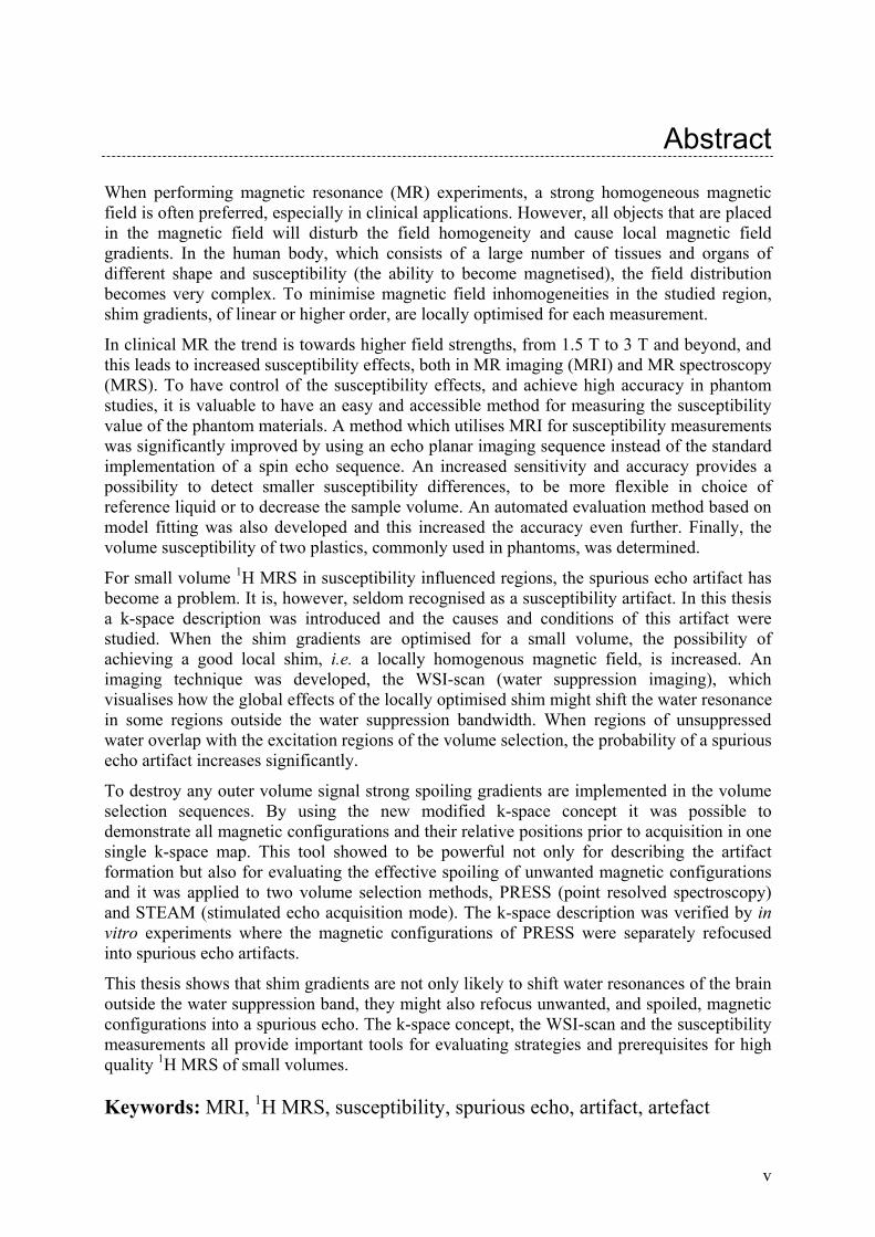
1. Introduction Magnetic resonance (MR) studies of hydrogen can be applied for a large variety of clinical applications, both in studies of anatomy and morphology with imaging (MRI) (Fig. 1a) and in non-invasive studies of cell and tissue metabolism using spectroscopy (MRS) (Fig. 1b). Common for many MR applications is the need for a strong homogeneous static magnetic field. The nuclear magnetisation of the hydrogen nuclei will be affected by this magnetic field, and a magnetisation that is aligned with the magnetic field will be created. Due to its angular momentum the nucleus will also start to precess and the precession frequency, i.e. the resonance frequency, ν, is determined by the Larmor equation,

B⋅= γν , (1)

where B is the magnetic field strength and γ is the gyromagnetic constant (42.58 MHz/T for 1H). By using an RF-pulse, with a bandwidth of frequencies around the resonance frequency, it is possible to perturb the magnetisation of the hydrogen nuclei and thereby cause an excitation. As a result a detectable signal is produced when the nuclei relaxes to equilibrium. This signal is called the FID (free induction decay). By applying linear magnetic field gradients in three dimensions, the magnetic field will become spatially dependent. This can be used for spatial encoding of an MR image, or for spatial selection of an MRS volume of interest (VOI) (1). The magnetic field gradients induce a spatial variation of phase and frequency and in conventional MRI the two in plane dimensions are therefore denoted phase and frequency encoding direction. The magnetic field gradients and the RF-pulses are combined into pulse sequences and by manipulating the pulse sequence a wide range of contrast phenomena are accomplished, resulting in many MR applications. T1, T2 and proton density are three fundamental properties of tissues and substances, and by changing the timing parameters of the imaging pulse sequence their influence on signal contrast between tissues in an MR image can be varied.

a b

Figure 1. a) A mid-sagittal T2 weighted MR image of the head. b) A 1H MR spectrum from grey matter in the occipital lobe in the brain. Commonly studied metabolites are marked with a number; 1) creatine, 2) glutamate +

1

glutamine, 3) myo-inositol, 4) choline and 5) N-acetylaspartate (NAA). A 1H MRS spectrum (Fig. 1b) contains a number of peaks where each peak corresponds to a molecule, or part of a molecule, that contains a 1H nucleus. The peak position is used to identify the molecule. The intensity, i.e. the integral, of the peak is proportional to the number of 1H nuclei contributing to the peak, i.e. proportional to the concentration of the molecule. The peak position, or frequency shift, is called the chemical shift and depends on how the 1H nuclei is shielded from the static magnetic field by electrons and other atoms (2). The effective magnetic field that the hydrogen nucleus experiences depends on the shielding constant, σ, which gives a modification of the Larmor frequency,

)1( σγν −⋅⋅= B . (2)

To eliminate the dependence of the chemical shift on the nominal static magnetic field strength, the chemical shift in a spectrum is usually given in parts per million (ppm) instead of Hertz.

)()()(

10)( 6

HzHzHzv

ppmreference

reference

νν

ν−

⋅= , (3)

where νreference is a chosen reference frequency, the zero point in spectrum, which often is tetramethyl-silane (TMS) for 1H MRS. When two adjacent materials have different susceptibility, i.e. difference in magnetisation by the applied magnetic field, a spatial variation of the magnetic field will arise in areas close to the border between the two materials. Hence, a difference in susceptibility leads to a local magnetic field gradient and according to the Larmor condition this gives a local variation in the resonance frequency. Since MR techniques utilise the frequency for both spatial encoding and molecule identification, a susceptibility induced frequency shift can result in measurement errors, displacement of signal and artifacts. Different pulse sequences can be more or less sensitive to the susceptibility effect. Thus, the susceptibility effects are mostly undesirable, but they can also be used for susceptibility determination with both MRI and MRS.

1.1 Magnetic Susceptibility

1.1.1 Physical properties There are several ways to express magnetic susceptibility and unfortunately no common standard have been agreed on in the scientific community. There are volume, molar and mass susceptibility, all with different dimensions and in the literature it is seldom stated which one is meant (3). Volume magnetic susceptibility (χV) is a dimensionless quantity that describes the contribution to the total magnetic flux density present, made by a substance when subjected to a magnetic field. For materials where the magnetisation, M (A/m), linearly depend on the strength of the magnetising field, H (A/m), the volume susceptibility is defined as

HM

V =χ . (4)

2

Molar susceptibility has the dimension m3/mol and is defined as

ρχχ VM

mW ⋅

= , (5)

where WM is the molar weight (kg/mol) and ρ the density (kg/m3). Mass susceptibility has the dimension m3/kg and is defined as

ρχχ V

g = . (6)

In this thesis and all four papers, the volume magnetic susceptibility is used. Diamagnetic materials have low negative volume magnetic susceptibility (e.g. water: χV = -9.03 ppm at 20°C), paramagnetic materials have low positive (e.g. titanium: χV = 182 ppm) and ferromagnetic materials have high positive susceptibility (e.g. iron: χV = 1011 ppm) (3). H is not commonly used in the clinical MR community. Instead the magnetic flux density, B, is used, often simply referred to as the magnetic field strength and with the unit Tesla (T).

( ) ( VHMHB )χμμ +⋅⋅=+⋅= 100 , (7)

where μ0 is the magnetic constant, i.e. the permeability of free space. When there is no material present, B and H will be redundant. But inside a material B will be affected by the susceptibility of the material. B0 is used to denote the external static magnetic field of an MR system.

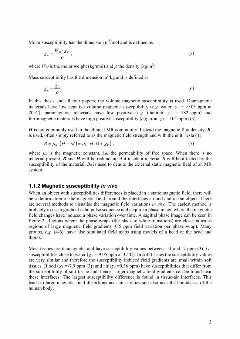
1.1.2 Magnetic susceptibility in vivo When an object with susceptibilities differences is placed in a static magnetic field, there will be a deformation of the magnetic field around the interfaces around and in the object. There are several methods to visualise the magnetic field variations in vivo. The easiest method is probably to use a gradient echo pulse sequence and acquire a phase image where the magnetic field changes have induced a phase variation over time. A sagittal phase image can be seen in figure 2. Regions where the phase wraps (the black to white transitions) are close indicates regions of large magnetic field gradients (0.5 ppm field variation per phase wrap). Many groups, e.g. (4-6), have also simulated field maps using models of a head or the head and thorax. Most tissues are diamagnetic and have susceptibility values between -11 and -7 ppm (3), i.e. susceptibilities close to water (χV =-9.05 ppm at 37°C). In soft tissues the susceptibility values are very similar and therefore the susceptibility induced field gradients are small within soft tissues. Blood (χV =-7.9 ppm (3)) and air (χV =0.36 ppm) have susceptibilities that differ from the susceptibility of soft tissue and, hence, larger magnetic field gradients can be found near these interfaces. The largest susceptibility difference is found in tissue-air interfaces. This leads to large magnetic field distortions near air cavities and also near the boundaries of the human body.

3

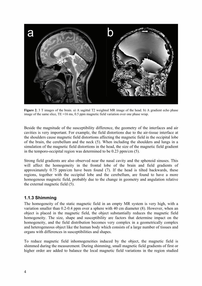
Figure 2. 3 T images of the brain. a) A sagittal T2 weighted MR image of the head. b) A gradient echo phase image of the same slice, TE =16 ms, 0.5 ppm magnetic field variation over one phase wrap. Beside the magnitude of the susceptibility difference, the geometry of the interfaces and air cavities is very important. For example, the field distortions due to the air-tissue interface at the shoulders cause magnetic field distortions affecting the magnetic field in the occipital lobe of the brain, the cerebellum and the neck (5). When including the shoulders and lungs in a simulation of the magnetic field distortions in the head, the size of the magnetic field gradient in the temporo-occipital region was determined to be 0.23 ppm/cm (5). Strong field gradients are also observed near the nasal cavity and the sphenoid sinuses. This will affect the homogeneity in the frontal lobe of the brain and field gradients of approximately 0.75 ppm/cm have been found (7). If the head is tilted backwards, these regions, together with the occipital lobe and the cerebellum, are found to have a more homogenous magnetic field, probably due to the change in geometry and angulation relative the external magnetic field (5).

1.1.3 Shimming The homogeneity of the static magnetic field in an empty MR system is very high, with a variation smaller than 0.2-0.4 ppm over a sphere with 40 cm diameter (8). However, when an object is placed in the magnetic field, the object substantially reduces the magnetic field homogeneity. The size, shape and susceptibility are factors that determine impact on the homogeneity, and the field distribution becomes very complex in a geometrically complex and heterogeneous object like the human body which consists of a large number of tissues and organs with differences in susceptibilities and shapes. To reduce magnetic field inhomogeneities induced by the object, the magnetic field is shimmed during the measurement. During shimming, small magnetic field gradients of first or higher order are added to balance the local magnetic field variations in the region studied

4

(the image volume for MRI and the VOI for MRS). The shim gradients must be optimised for each measurement situation. There are two principal ways to perform shimming, iterative or calculative. Iterative FID shimming is an optimisation method, which by repetitive measurements searches for the shim settings that give the maximal time integral of the magnitude of the FID signal (2). A faster optimisation can be achieved with a calculative method where the shim settings are calculated out of the guidance of a few measurement, e.g. FASTMAP (9,10). In the FASTMAP method the B0 magnetic field variations along several lines (pencil beams) in different directions through the studied region, are determined by measuring the phase variation along these lines. The optimal superposition of the eight orthogonal spherical harmonics of the first and second order shim coils is then found to match the field variations from the pencil beam scans. All shim gradients are centred in the iso-centre of the magnet and for higher order shimming this means that in any off-centre position, the spherical harmonics will all interact (11). Positions off-centre on a second order gradient will require the use of a linear gradient to balance the linear component of the second order gradient. Therefore, when using second order shimming for a VOI positioned off-centre, the linear shim gradient should both balance the linear component of the magnetic field over the VOI and the linear component of the second order shim gradient. The shim magnetic field gradients are optimised to minimise local differences but are added globally. This can result in larger magnetic field inhomogeneities in regions outside the one studied. By using higher order shimming, more complex inhomogeneities can be balanced, but they will also lead to a more complex global magnetic field distribution outside the studied region. For VOIs positioned off-centre, the linear gradient used to balance the linear component of the second order shim gradient inside the VOI, will add globally and can cause a considerably large magnetic field gradient outside the VOI.

1.2 MRI and Susceptibility In MRI, a susceptibility difference which induces differences in the magnetic field strengths and hence frequency shifts, will affect the spatial encoding (1). The resulting signal displacements can lead to accumulation as well as dispersion of the signal and appear as intensity spots and black spots in the image. Different pulse sequences are differently sensitive to susceptibility and the magnitude of the artifacts can vary extremely, sometimes the artifacts are subtle enough to be masked by the tissue structures in the image and sometimes the entire image is distorted.

1.2.1 Pulse sequences

k-space concept The object is represented in k-space by its Fourier transform. During scanning, the point of signal collection is moved around in k-space by the magnetic field gradients (Eq. 8) of the MR system according to the pulse sequence (12),

5

∫=t

dtt0

)(Gk γ , (8)

where γ is the gyromagnetic constant (cf. Eq. 1), G the linear magnetic field gradient and t the time. The total k-space trajectory depends on both gradients and RF-pulses. For imaging, most pulse sequences are repeated as many times as necessary to complete sampling of signal from the central area in k-space, determined by the desired spatial resolution and field of view. Depending on the acquisition strategy in k-space, the susceptibility artifact will have different appearance and distinction in the image. For conventional sampling, the main parameter that affects the size of the artifact is the bandwidth per pixel. Bandwidth per pixel is the frequency difference from one pixel to the next, which, in turn, is determined by the inverse of the time elapsed between adjacent k-space samples. The smaller the bandwidth per pixel, the greater the size of the susceptibility artifact will be.

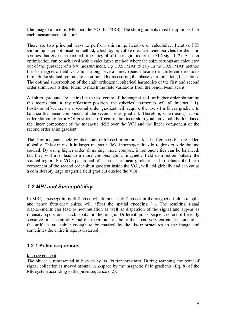
Spin-echo (SE) The spin echo sequence, SE, is one of the most common and simplest pulse sequences. The sequence and its k-space trajectory are shown in figure 3. It has a 180° RF-pulse that refocuses the spins at the echo time and thereby diminishes the phase shifts in the voxel, which are caused by local static magnetic field gradients. This refocusing 180° RF-pulse makes the SE pulse sequence less sensitive to susceptibility effects. All sample points on the same line along the phase encoding direction are acquired at the same point in time after excitation, implying infinite bandwidth per pixel in this direction. Therefore, the SE images are only affected by susceptibility differences in the frequency encoding direction. A faster version of the SE is the turbo spin echo (TSE) pulse sequence. TSE utilises several equidistant 180° RF-pulses to create several spin echoes and thereby acquire several k-space lines during one repetition time (TR).

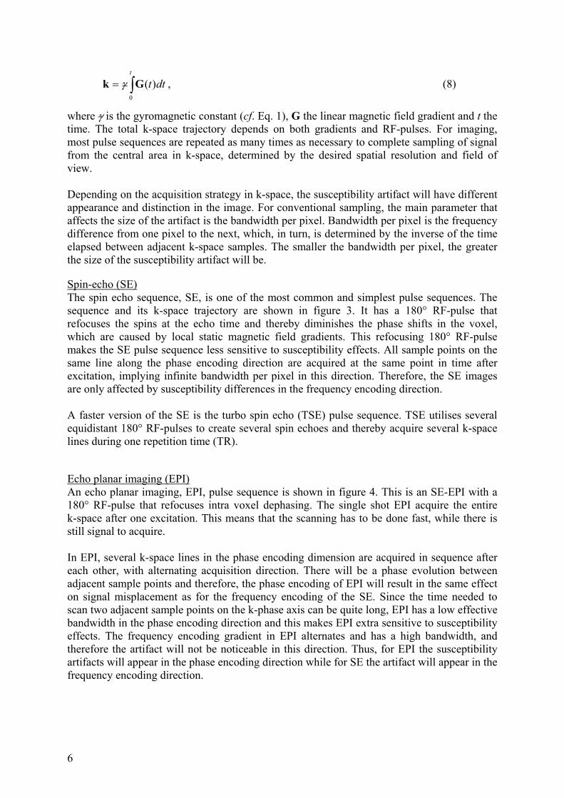
Echo planar imaging (EPI) An echo planar imaging, EPI, pulse sequence is shown in figure 4. This is an SE-EPI with a 180° RF-pulse that refocuses intra voxel dephasing. The single shot EPI acquire the entire k-space after one excitation. This means that the scanning has to be done fast, while there is still signal to acquire. In EPI, several k-space lines in the phase encoding dimension are acquired in sequence after each other, with alternating acquisition direction. There will be a phase evolution between adjacent sample points and therefore, the phase encoding of EPI will result in the same effect on signal misplacement as for the frequency encoding of the SE. Since the time needed to scan two adjacent sample points on the k-phase axis can be quite long, EPI has a low effective bandwidth in the phase encoding direction and this makes EPI extra sensitive to susceptibility effects. The frequency encoding gradient in EPI alternates and has a high bandwidth, and therefore the artifact will not be noticeable in this direction. Thus, for EPI the susceptibility artifacts will appear in the phase encoding direction while for SE the artifact will appear in the frequency encoding direction.

6

Figure 3. A spin echo pulse sequence and its trajectory, a-e, in k-space. a to e illustrates one phase encoding step and the sequence is repeated until all phase encoding steps are acquired. All sample points on the same line along the phase encoding direction are acquired at the same point in time after excitation, implying infinite bandwidth per pixel in this direction.

Figure 4. A single shot echo planar imaging pulse sequence and its trajectory, a-e, in k-space. a to e illustrates the path of the trajectory and the whole k-space is acquired in one excitation. All k-space lines in the phase encoding dimension are acquired in sequence. Therefore, there will be a phase evolution between adjacent sample points, and a low effective bandwidth, in phase encoding direction.

1.2.2 Susceptibility measurement The geometric susceptibility artifact can be utilised for susceptibility measurements to determine the susceptibility value for different materials (13). When imaging a coaxial cylinder, perpendicular to the magnetic field, the susceptibility difference between the inner and outer compartment causes the circular cross section of the inner compartment to appear as a spear-head. The size of the artifact is related to the susceptibility difference between the inner and outer compartment. Beuf et al. utilised a SE sequence for the susceptibility measurements (13). However, the high bandwidth of the SE sequence, which means low sensitivity to susceptibility effects, makes the range of susceptibilities possible to measure highly dependent on the susceptibility of the reference liquid. The susceptibility of plastics and tissue like materials is very difficult to measure using SE.

7

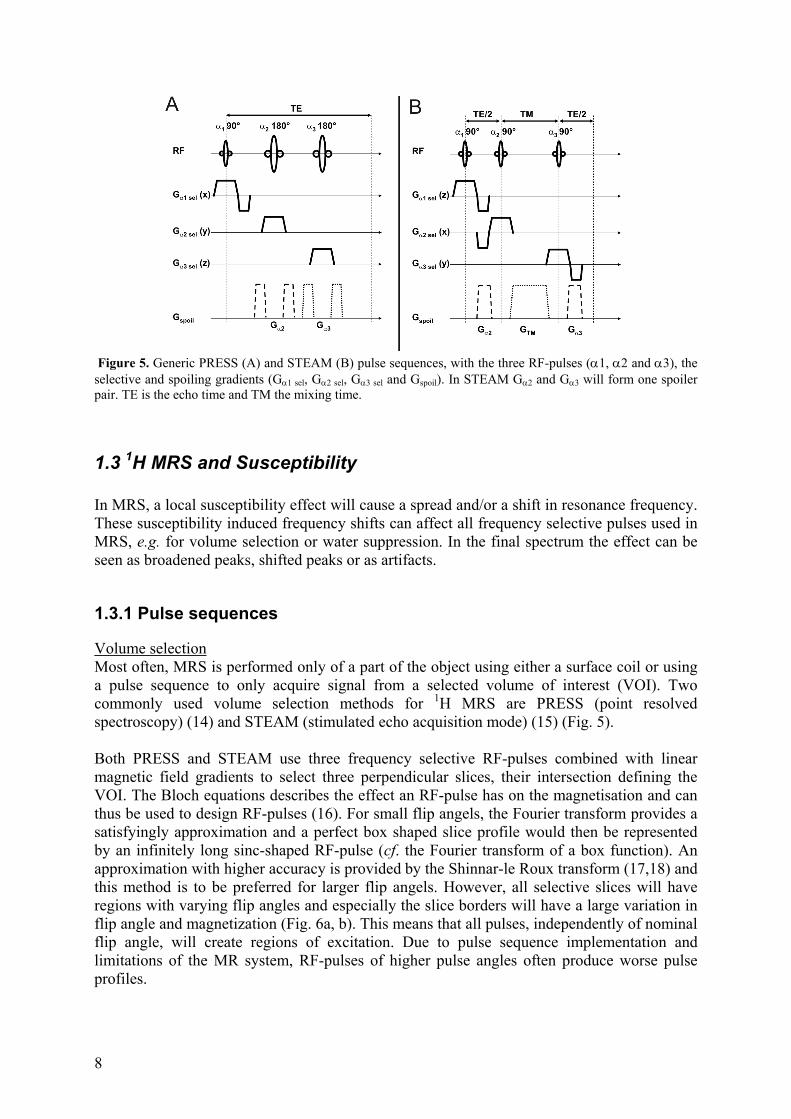
Figure 5. Generic PRESS (A) and STEAM (B) pulse sequences, with the three RF-pulses (α1, α2 and α3), the selective and spoiling gradients (Gα1 sel, Gα2 sel, Gα3 sel and Gspoil). In STEAM Gα2 and Gα3 will form one spoiler pair. TE is the echo time and TM the mixing time.

1.3 1H MRS and Susceptibility In MRS, a local susceptibility effect will cause a spread and/or a shift in resonance frequency. These susceptibility induced frequency shifts can affect all frequency selective pulses used in MRS, e.g. for volume selection or water suppression. In the final spectrum the effect can be seen as broadened peaks, shifted peaks or as artifacts.

1.3.1 Pulse sequences

Volume selection Most often, MRS is performed only of a part of the object using either a surface coil or using a pulse sequence to only acquire signal from a selected volume of interest (VOI). Two commonly used volume selection methods for 1H MRS are PRESS (point resolved spectroscopy) (14) and STEAM (stimulated echo acquisition mode) (15) (Fig. 5). Both PRESS and STEAM use three frequency selective RF-pulses combined with linear magnetic field gradients to select three perpendicular slices, their intersection defining the VOI. The Bloch equations describes the effect an RF-pulse has on the magnetisation and can thus be used to design RF-pulses (16). For small flip angels, the Fourier transform provides a satisfyingly approximation and a perfect box shaped slice profile would then be represented by an infinitely long sinc-shaped RF-pulse (cf. the Fourier transform of a box function). An approximation with higher accuracy is provided by the Shinnar-le Roux transform (17,18) and this method is to be preferred for larger flip angels. However, all selective slices will have regions with varying flip angles and especially the slice borders will have a large variation in flip angle and magnetization (Fig. 6a, b). This means that all pulses, independently of nominal flip angle, will create regions of excitation. Due to pulse sequence implementation and limitations of the MR system, RF-pulses of higher pulse angles often produce worse pulse profiles.

8

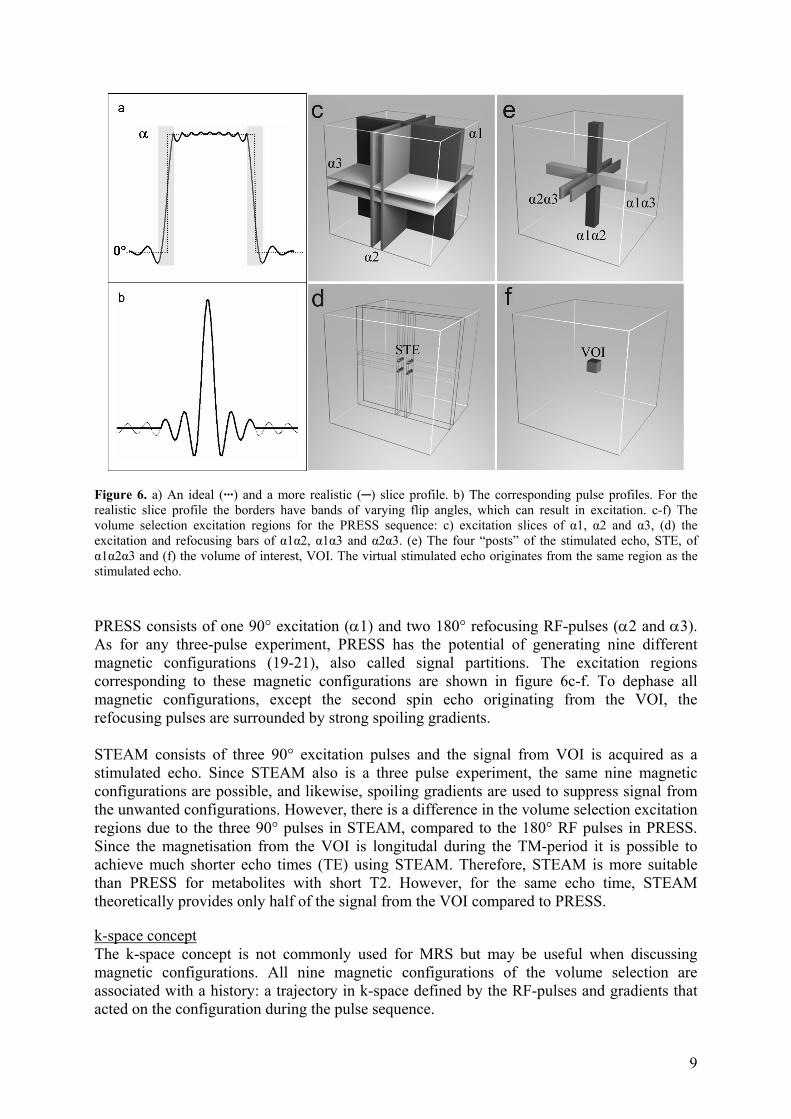
Figure 6. a) An ideal (···) and a more realistic (─) slice profile. b) The corresponding pulse profiles. For the realistic slice profile the borders have bands of varying flip angles, which can result in excitation. c-f) The volume selection excitation regions for the PRESS sequence: c) excitation slices of α1, α2 and α3, (d) the excitation and refocusing bars of α1α2, α1α3 and α2α3. (e) The four “posts” of the stimulated echo, STE, of α1α2α3 and (f) the volume of interest, VOI. The virtual stimulated echo originates from the same region as the stimulated echo. PRESS consists of one 90° excitation (α1) and two 180° refocusing RF-pulses (α2 and α3). As for any three-pulse experiment, PRESS has the potential of generating nine different magnetic configurations (19-21), also called signal partitions. The excitation regions corresponding to these magnetic configurations are shown in figure 6c-f. To dephase all magnetic configurations, except the second spin echo originating from the VOI, the refocusing pulses are surrounded by strong spoiling gradients. STEAM consists of three 90° excitation pulses and the signal from VOI is acquired as a stimulated echo. Since STEAM also is a three pulse experiment, the same nine magnetic configurations are possible, and likewise, spoiling gradients are used to suppress signal from the unwanted configurations. However, there is a difference in the volume selection excitation regions due to the three 90° pulses in STEAM, compared to the 180° RF pulses in PRESS. Since the magnetisation from the VOI is longitudal during the TM-period it is possible to achieve much shorter echo times (TE) using STEAM. Therefore, STEAM is more suitable than PRESS for metabolites with short T2. However, for the same echo time, STEAM theoretically provides only half of the signal from the VOI compared to PRESS.

k-space concept The k-space concept is not commonly used for MRS but may be useful when discussing magnetic configurations. All nine magnetic configurations of the volume selection are associated with a history: a trajectory in k-space defined by the RF-pulses and gradients that acted on the configuration during the pulse sequence.

9

Phase cycling Phase cycling is a method used to eliminate unwanted signals due to, e.g. DC offsets, spectrometer imbalances, coherent noise and/or multi pulse artifacts, on the basis of their phase property. The unwanted signals might have different phase behaviour compared to the desired signal, and by phase cycling of the RF-pulses and the receiver, unwanted signals may cancel, while the desired signal is accumulated. Phase cycling can be performed with different number of steps and the more steps utilised, the more unwanted signals are cancelled (22-24).

Water suppression The in vivo MRS signal from the molecules of interest is usually much weaker than the water signal, approximately by a factor of 1/10000. Therefore, water suppression techniques are used to spoil the water signal before acquisition. Water suppression can be achieved in several different ways but most methods utilise the difference in chemical shift between water and other resonances. The most commonly used water suppression method is CHESS (chemical shift selective), which works by exciting only a small bandwidth of frequencies around the water resonance and then spoil this signal using strong gradients before VOI localisation and signal acquisition (25). To get a more efficient water suppression, the CHESS sequence is often repeated up to three times before volume selection (2). The water suppression is performed without volume selection and will preferably spoil the water signal over the entire object. But if local magnetic field gradients or shim gradients are present, these can act as selective gradients by shifting the water resonance outside the water suppression bandwidth and thereby create regions with unsuppressed water.

1.3.2 The spurious echo artifact The spurious echo artifact is one of the susceptibility artifacts in MRS. Probably all MRS users experience it more or less frequently. It appears at various and unpredictable positions in spectrum as a complex structure with limited bandwidth (Fig. 7). The artifact have been referred to as ghosts, wiggles, beating signal, spurious peaks, unwanted echoes, spurious echoes etc. and has to some extent been described (26-29). However, although recognised for a long time, it seems as if the artifact now appears more frequently. In a retrospective study of MRS data at our site, a spurious artifact could be found in approximately 40 % of the spectra, when studied carefully. This does not mean that all of these spectra were unusable. Caution must be taken when interpreting spectral data if the artifact overlaps with peaks of the molecules of interest and therefore interfere with the result. The artifact is often easiest observed in the residual spectrum, i.e. the difference between the measured spectrum and a fitted model spectrum. Four experimental conditions must concur to give rise to a spurious echo artifact (26,27).

1. There must exist unsuppressed water, e.g. due to a static magnetic field gradient that shifts water resonances outside the water suppression band.

2. There must be an excitation of the unsuppressed water. 3. This water signal must be refocused into an echo during the signal acquisition. 4. The phase cancellation of unwanted signals in the phase cycling must fail.

10

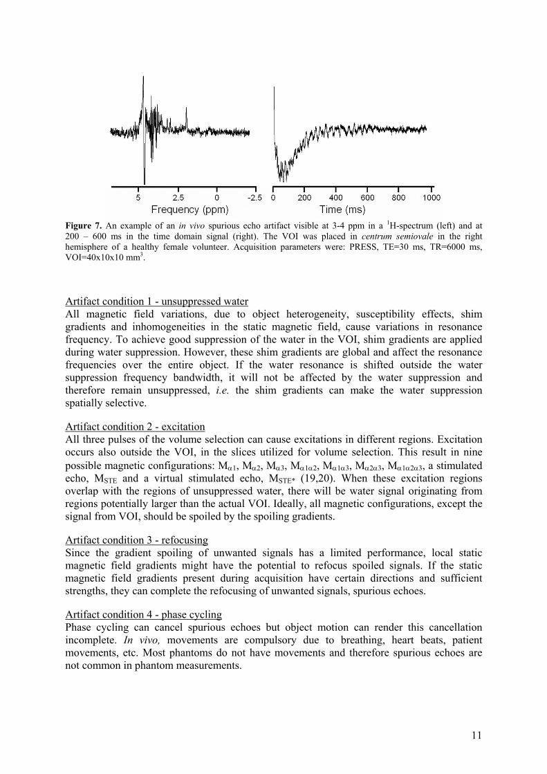
Figure 7. An example of an in vivo spurious echo artifact visible at 3-4 ppm in a 1H-spectrum (left) and at 200 – 600 ms in the time domain signal (right). The VOI was placed in centrum semiovale in the right hemisphere of a healthy female volunteer. Acquisition parameters were: PRESS, TE=30 ms, TR=6000 ms, VOI=40x10x10 mm3.

Artifact condition 1 - unsuppressed water All magnetic field variations, due to object heterogeneity, susceptibility effects, shim gradients and inhomogeneities in the static magnetic field, cause variations in resonance frequency. To achieve good suppression of the water in the VOI, shim gradients are applied during water suppression. However, these shim gradients are global and affect the resonance frequencies over the entire object. If the water resonance is shifted outside the water suppression frequency bandwidth, it will not be affected by the water suppression and therefore remain unsuppressed, i.e. the shim gradients can make the water suppression spatially selective.

Artifact condition 2 - excitation All three pulses of the volume selection can cause excitations in different regions. Excitation occurs also outside the VOI, in the slices utilized for volume selection. This result in nine possible magnetic configurations: Mα1, Mα2, Mα3, Mα1α2, Mα1α3, Mα2α3, Mα1α2α3, a stimulated echo, MSTE and a virtual stimulated echo, MSTE* (19,20). When these excitation regions overlap with the regions of unsuppressed water, there will be water signal originating from regions potentially larger than the actual VOI. Ideally, all magnetic configurations, except the signal from VOI, should be spoiled by the spoiling gradients.

Artifact condition 3 - refocusing Since the gradient spoiling of unwanted signals has a limited performance, local static magnetic field gradients might have the potential to refocus spoiled signals. If the static magnetic field gradients present during acquisition have certain directions and sufficient strengths, they can complete the refocusing of unwanted signals, spurious echoes.

Artifact condition 4 - phase cycling Phase cycling can cancel spurious echoes but object motion can render this cancellation incomplete. In vivo, movements are compulsory due to breathing, heart beats, patient movements, etc. Most phantoms do not have movements and therefore spurious echoes are not common in phantom measurements.

11

1.3.3 Susceptibility measurements The susceptibility effect in MRS can be used to measure the susceptibility of liquids (30). This method can not be used for solid materials since the signal diminishes too fast, i.e. the T2 value for solid materials are too small. A long circular cylinder placed parallel to the magnetic field and an identical cylinder placed perpendicular to the magnetic field will induce different susceptibility effects and the induced frequency shift can be utilized to determine the susceptibility of the liquid inside the cylinders (13).

12

2. Aim The aim of this thesis was to study susceptibility effects in MRI and 1H MRS, to describe and study the spurious echo artifact in 1H MRS and to utilise the susceptibility effects in MRI to measure susceptibility in phantom materials. Specifically, the aim of this work was to

- describe the theoretical considerations of the spurious echo artifact in MRS using a k-space concept.

- verify the k-space description and explore and characterise the spurious echo by in

vitro measurements.

- study different spoiling schemes for PRESS and STEAM using the k-space concept and examine strategies to minimise or reduce the risk of a spurious echo artifact in 1H MRS.

- study the effects of shimming on water suppression performance for small volumes in

in vivo 1H MRS and to compare the impact of first and second order shimming and different shimming optimization methods, and

- improve the sensitivity and accuracy of susceptibility determination to facilitate

measurements on materials commonly used for MR phantoms, e.g. plastics.

13

14

3. Material & Methods 3.1 Spurious Echo Artifact (paper I, II and III)

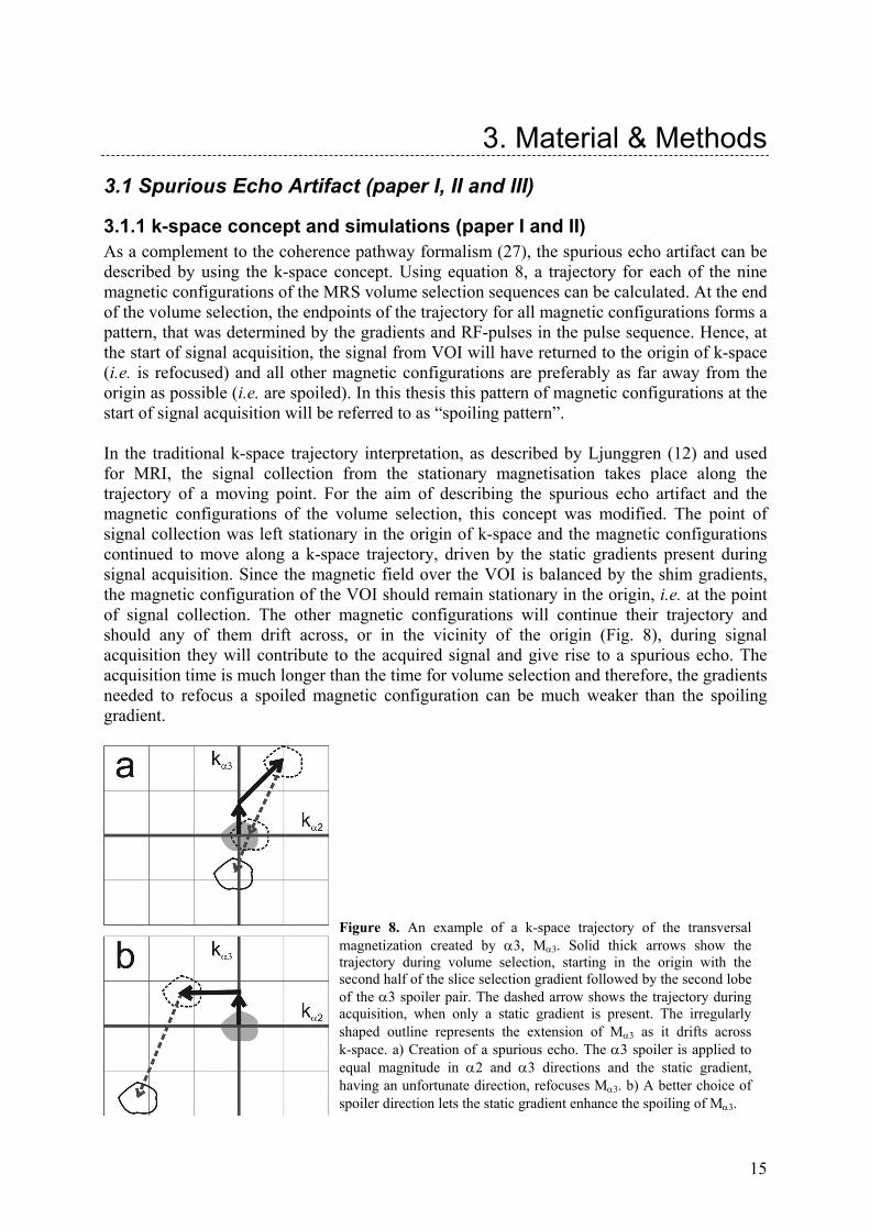
3.1.1 k-space concept and simulations (paper I and II) As a complement to the coherence pathway formalism (27), the spurious echo artifact can be described by using the k-space concept. Using equation 8, a trajectory for each of the nine magnetic configurations of the MRS volume selection sequences can be calculated. At the end of the volume selection, the endpoints of the trajectory for all magnetic configurations forms a pattern, that was determined by the gradients and RF-pulses in the pulse sequence. Hence, at the start of signal acquisition, the signal from VOI will have returned to the origin of k-space (i.e. is refocused) and all other magnetic configurations are preferably as far away from the origin as possible (i.e. are spoiled). In this thesis this pattern of magnetic configurations at the start of signal acquisition will be referred to as “spoiling pattern”. In the traditional k-space trajectory interpretation, as described by Ljunggren (12) and used for MRI, the signal collection from the stationary magnetisation takes place along the trajectory of a moving point. For the aim of describing the spurious echo artifact and the magnetic configurations of the volume selection, this concept was modified. The point of signal collection was left stationary in the origin of k-space and the magnetic configurations continued to move along a k-space trajectory, driven by the static gradients present during signal acquisition. Since the magnetic field over the VOI is balanced by the shim gradients, the magnetic configuration of the VOI should remain stationary in the origin, i.e. at the point of signal collection. The other magnetic configurations will continue their trajectory and should any of them drift across, or in the vicinity of the origin (Fig. 8), during signal acquisition they will contribute to the acquired signal and give rise to a spurious echo. The acquisition time is much longer than the time for volume selection and therefore, the gradients needed to refocus a spoiled magnetic configuration can be much weaker than the spoiling gradient.

Figure 8. An example of a k-space trajectory of the transversal magnetization created by α3, Mα3. Solid thick arrows show the trajectory during volume selection, starting in the origin with the second half of the slice selection gradient followed by the second lobe of the α3 spoiler pair. The dashed arrow shows the trajectory during acquisition, when only a static gradient is present. The irregularly shaped outline represents the extension of Mα3 as it drifts across k-space. a) Creation of a spurious echo. The α3 spoiler is applied to equal magnitude in α2 and α3 directions and the static gradient, having an unfortunate direction, refocuses Mα3. b) A better choice of spoiler direction lets the static gradient enhance the spoiling of Mα3.

15

Computer simulations were set up to analyse and illustrate the consequences of the slice profile and the k-space considerations of the spurious echo artifact. The simulation was setup to mimic a single voxel 1H MRS measurement in the brain in a clinical 1.5 T MR scanner. For PRESS one large VOI, 30x30x30 mm3, and one small VOI, 10x10x10 mm3, were examined. Echo time, and approximate duration of volume selection, was 30 ms. Numerical values for other sequence parameters were chosen to be representative for a clinical MR system for in vivo application in the brain. The three RF-pulses, α1, α2 and α3, were sinc shaped, truncated after the fourth pair of side lobes and weighted with a Hann window (also known as Hanning) (31). Pulse durations were 2.5 ms for α1 (90° flip angle) and 5 ms for α2 and α3 (180° flip angle). Slice profiles were calculated using the forward Shinnar-le Roux transformation (17,18). The content of spatial frequencies in the slice profiles, i.e. the extension of the magnetic configuration in k-space, was calculated by means of the Fourier transform and evaluated at the levels 10-1 and 10-5 of maximum in the modulus of the slice profile spectrum. The levels 10-1 and 10-5 indicate where metabolite signal and unsuppressed water signal, respectively, would be much less than e.g. N-acetyl-aspartate (NAA) signal in magnitude Signals below these levels were regarded as adequately spoiled, i.e. too weak to interfere with the signal from the VOI. For the small VOI, the slice selection gradients were 10 mT/m for the α1 slice and 3.6 mT/m for the α2 and α3 slices. Consequently, the magnitude of the k-vector of the selection gradients for the α2 and α3 slices was 766 m-1 each. The corresponding values for the large VOI were 3.3 mT/m, 1.2 mT/m and 255 m-1. The k-vector for one pair of spoiler gradients was 2x1000 m-1 for both VOI sizes. Finally, the extensions of the frequency spectra of the corresponding slice profiles were combined with the k-space pattern for the model PRESS sequence. Different spoiling patterns were investigated for both PRESS and STEAM. For PRESS, the sign of the spoiling gradients were altered. Only the components in the kα2 and kα3 directions of the spoiler gradient pairs were changed, and the slice selection gradients were omitted. This gives four alternative directions for the α2 spoiler pair: (kα2, kα3) = [(+1000m-1, +1000m-1), (+1000m-1, -1000m-1), (-1000m-1, +1000m-1), (-1000m-1, -1000m-1)]. The α3 spoiler pair can have any of these four directions for each alternative of the α2 spoilers, resulting in a total of 16 combinations of spoiler directions. For STEAM only the mixing time spoiling gradient (GTM) was altered, both by a change in strength and direction. The α2-α3 spoiler pair (cf. Gα2 and Gα3 in Fig. 5) was set to 2x1000 m-1. Three values of GTM strength were compared, 1000 m-1, 2000 m-1 and 3000 m-1. Altering the direction of the GTM only the components in the kα2 and kα3 directions of the spoiler gradient pairs were changed, the slice selection gradients were omitted. This gives four alternative directions for the TM spoiler pair: (kα2, kα3) = [(+3000m-1, +3000m-1), (+3000m-1, -3000m-1), (-3000m-1, +3000m-1), (-3000m-1, -3000m-1)].

16

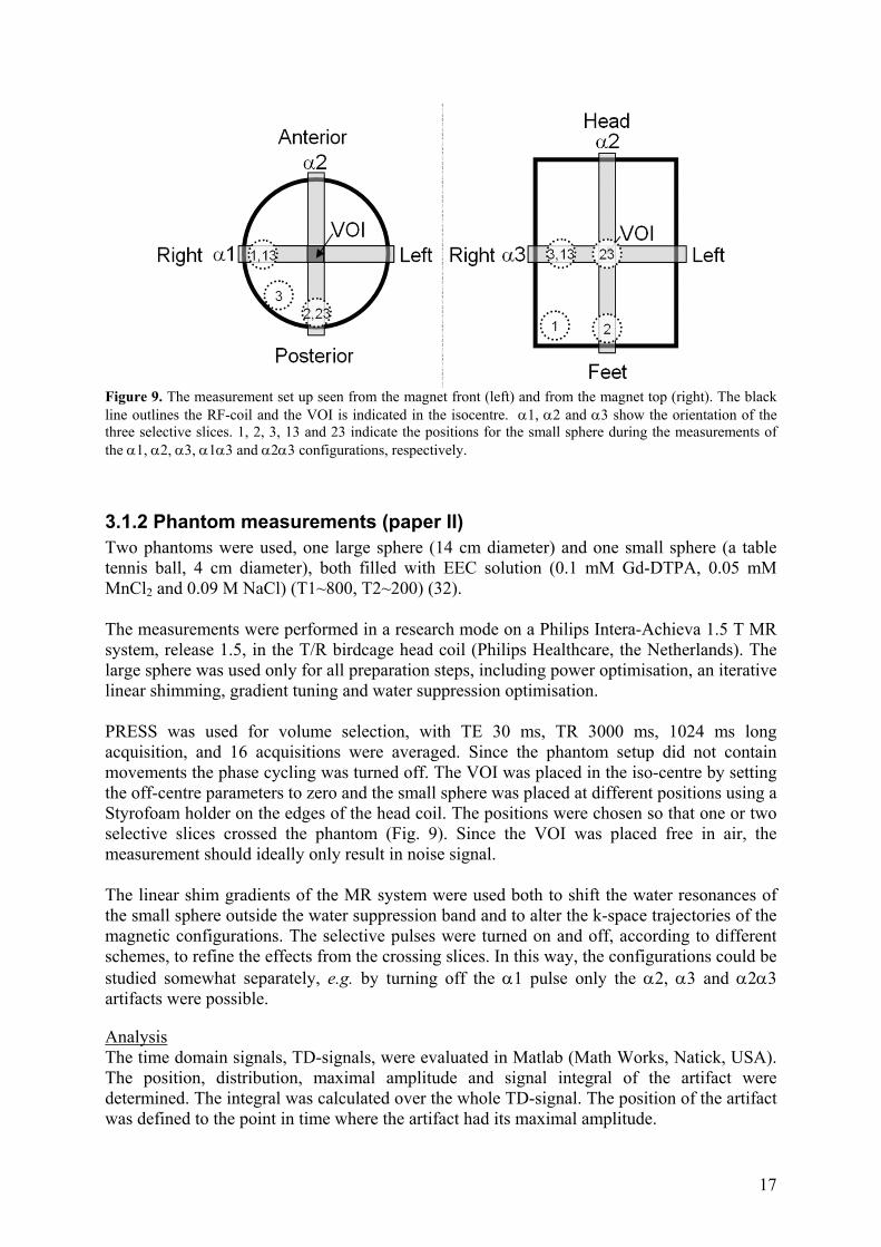
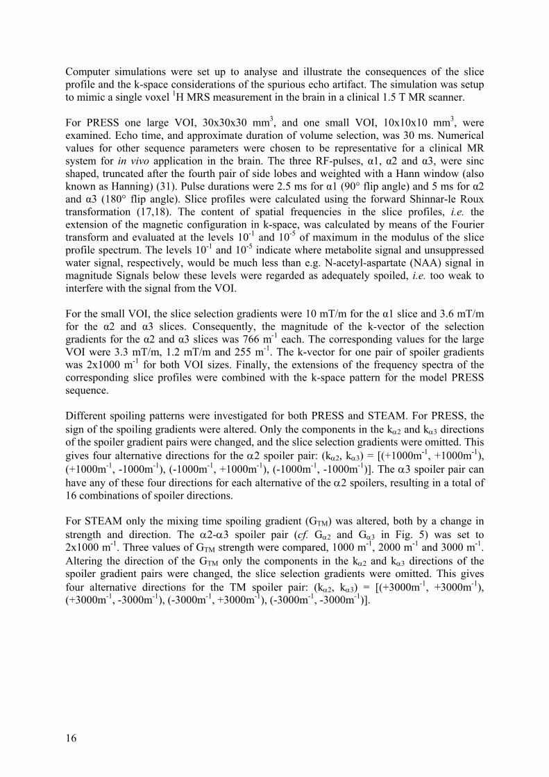
Figure 9. The measurement set up seen from the magnet front (left) and from the magnet top (right). The black line outlines the RF-coil and the VOI is indicated in the isocentre. α1, α2 and α3 show the orientation of the three selective slices. 1, 2, 3, 13 and 23 indicate the positions for the small sphere during the measurements of the α1, α2, α3, α1α3 and α2α3 configurations, respectively.

3.1.2 Phantom measurements (paper II) Two phantoms were used, one large sphere (14 cm diameter) and one small sphere (a table tennis ball, 4 cm diameter), both filled with EEC solution (0.1 mM Gd-DTPA, 0.05 mM MnCl2 and 0.09 M NaCl) (T1~800, T2~200) (32). The measurements were performed in a research mode on a Philips Intera-Achieva 1.5 T MR system, release 1.5, in the T/R birdcage head coil (Philips Healthcare, the Netherlands). The large sphere was used only for all preparation steps, including power optimisation, an iterative linear shimming, gradient tuning and water suppression optimisation. PRESS was used for volume selection, with TE 30 ms, TR 3000 ms, 1024 ms long acquisition, and 16 acquisitions were averaged. Since the phantom setup did not contain movements the phase cycling was turned off. The VOI was placed in the iso-centre by setting the off-centre parameters to zero and the small sphere was placed at different positions using a Styrofoam holder on the edges of the head coil. The positions were chosen so that one or two selective slices crossed the phantom (Fig. 9). Since the VOI was placed free in air, the measurement should ideally only result in noise signal. The linear shim gradients of the MR system were used both to shift the water resonances of the small sphere outside the water suppression band and to alter the k-space trajectories of the magnetic configurations. The selective pulses were turned on and off, according to different schemes, to refine the effects from the crossing slices. In this way, the configurations could be studied somewhat separately, e.g. by turning off the α1 pulse only the α2, α3 and α2α3 artifacts were possible.

Analysis The time domain signals, TD-signals, were evaluated in Matlab (Math Works, Natick, USA). The position, distribution, maximal amplitude and signal integral of the artifact were determined. The integral was calculated over the whole TD-signal. The position of the artifact was defined to the point in time where the artifact had its maximal amplitude.

17

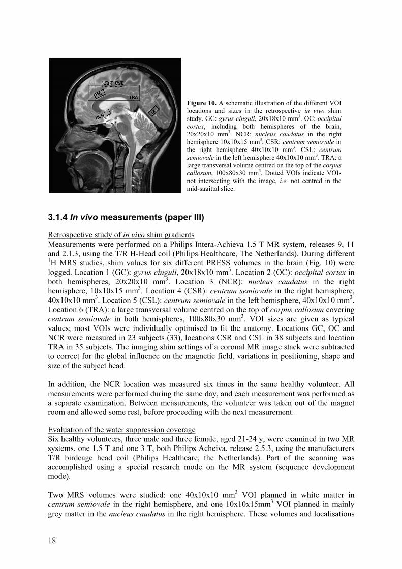
Figure 10. A schematic illustration of the different VOI locations and sizes in the retrospective in vivo shim study. GC: gyrus cinguli, 20x18x10 mm3. OC: occipital cortex, including both hemispheres of the brain, 20x20x10 mm3. NCR: nucleus caudatus in the right hemisphere 10x10x15 mm3. CSR: centrum semiovale in the right hemisphere 40x10x10 mm3. CSL: centrum semiovale in the left hemisphere 40x10x10 mm3. TRA: a large transversal volume centred on the top of the corpus callosum, 100x80x30 mm3. Dotted VOIs indicate VOIs not intersecting with the image, i.e. not centred in the mid-sagittal slice.

3.1.4 In vivo measurements (paper III)

Retrospective study of in vivo shim gradients Measurements were performed on a Philips Intera-Achieva 1.5 T MR system, releases 9, 11 and 2.1.3, using the T/R H-Head coil (Philips Healthcare, The Netherlands). During different 1H MRS studies, shim values for six different PRESS volumes in the brain (Fig. 10) were logged. Location 1 (GC): gyrus cinguli, 20x18x10 mm3. Location 2 (OC): occipital cortex in both hemispheres, 20x20x10 mm3. Location 3 (NCR): nucleus caudatus in the right hemisphere, 10x10x15 mm3. Location 4 (CSR): centrum semiovale in the right hemisphere, 40x10x10 mm3. Location 5 (CSL): centrum semiovale in the left hemisphere, 40x10x10 mm3. Location 6 (TRA): a large transversal volume centred on the top of corpus callosum covering centrum semiovale in both hemispheres, 100x80x30 mm3. VOI sizes are given as typical values; most VOIs were individually optimised to fit the anatomy. Locations GC, OC and NCR were measured in 23 subjects (33), locations CSR and CSL in 38 subjects and location TRA in 35 subjects. The imaging shim settings of a coronal MR image stack were subtracted to correct for the global influence on the magnetic field, variations in positioning, shape and size of the subject head. In addition, the NCR location was measured six times in the same healthy volunteer. All measurements were performed during the same day, and each measurement was performed as a separate examination. Between measurements, the volunteer was taken out of the magnet room and allowed some rest, before proceeding with the next measurement.

Evaluation of the water suppression coverage Six healthy volunteers, three male and three female, aged 21-24 y, were examined in two MR systems, one 1.5 T and one 3 T, both Philips Acheiva, release 2.5.3, using the manufacturers T/R birdcage head coil (Philips Healthcare, the Netherlands). Part of the scanning was accomplished using a special research mode on the MR system (sequence development mode). Two MRS volumes were studied: one 40x10x10 mm3 VOI planned in white matter in centrum semiovale in the right hemisphere, and one 10x10x15mm3 VOI planned in mainly grey matter in the nucleus caudatus in the right hemisphere. These volumes and localisations

18

correspond to the CSR and NCR locations in the retrospective shim study described above. PRESS was used for MRS volume selection, TE=30 ms, TR=2000 ms, 1024 ms signal acquisition and 128 measurements were averaged (NSA) for the larger CSR VOI and 128 or 256 NSA for the smaller NCR VOI. All MRS measurements were separately optimised regarding e.g. water suppression and shimming. For each measurement a 16 NSA non water suppressed reference spectrum was acquired for eddy current correction of the water suppressed spectra. The water suppression had a 1.1 ppm bandwidth. For the 1.5 T system, two different linear shimming optimisation methods were compared for each VOI localisation; one iterative and one calculative method called pencil beam. On the 3 T system, first and second order calculative shimming using pencil beams were compared for each VOI localisation. The iterative shim optimisation was performed on the VOI. For the calculative shimming, nine projections were used, the shim optimisation volume had never any dimension smaller than 25 mm and all spherical harmonics were fitted simultaneously. To visualize regions unaffected by the water suppression, an MRI scan which had the MRS water suppression added as a prepulse (RF-pulses and gradients) was developed. This scan is denoted “WSI-scan” (water suppression imaging). The WSI-scan was based on a single shot turbo spin echo sequence (TSE) with TE=70 ms and covered the entire head. For the 1.5 T system, the in-plane resolution was 3x5 mm2, slice thickness was 5 mm, 1 mm slice gap and an automatic linear shimming was performed with a first scan as a reference MRI-shim. On the 3 T system the WSI-scan in-plane resolution was 3x3 mm2, 3 mm slice thickness and 1 mm slice gap. Second order shimming was performed on a volume covering the entire head for reference MRI-shim values. The water suppression prepulse was a double CHESS sequence, where the second CHESS pulse was optimised for each VOI localisation. The WSI-scan time was approximately 22 s on both MR systems. Each MRS measurement was followed by a WSI-scan using the same shim setting and the same water suppression RF pulse angles. Thereby, the WSI-scan could visualise the water suppression regions for each MRS measurement. In addition, a WSI-scan which used the MRI optimized shims was acquired and for five of the twelve measurements a water spectrum (NSA=16) using the MRI shim settings was acquired (two 1.5 T and three 3 T). Also, a reference WSI-scan without water suppression was performed with MRI-shim values and with the water suppression RF-pulses angles set to zero. This pulse sequence was otherwise identical with the other WSI-scans. The WSI-scans were evaluated visually to give a qualitative description of the regions containing unsuppressed water, i.e. regions where the water resonance was shifted outside the water suppression bandwidth and therefore not affected by the water suppression. The WSI-scans were also quantitatively evaluated using image evaluation software MIPAV (34), where all images were segmented into binary masks showing voxels as either signalling or suppressed. The fractional suppressed volume in percent, Vsuppressed, was calculated using equation 9.

100⋅−

=reference

WSIreferencesuppressed V

VVV , (9)

where Vreference is the signalling volume of the binary mask for the reference scans where no water suppression was used and VWSI is the signalling volume of the binary mask for the WSI-scan.

19

The spectra were evaluated using both jMRUI (35) and LCmodel (36) to study the occurrence of spurious echo artifacts. jMRUI was also used to determine the FWHM of the reference water peak as a measure of quality of the VOI shim.

3.2 Susceptibility Measurements (paper IV)

3.2.1 Measurements

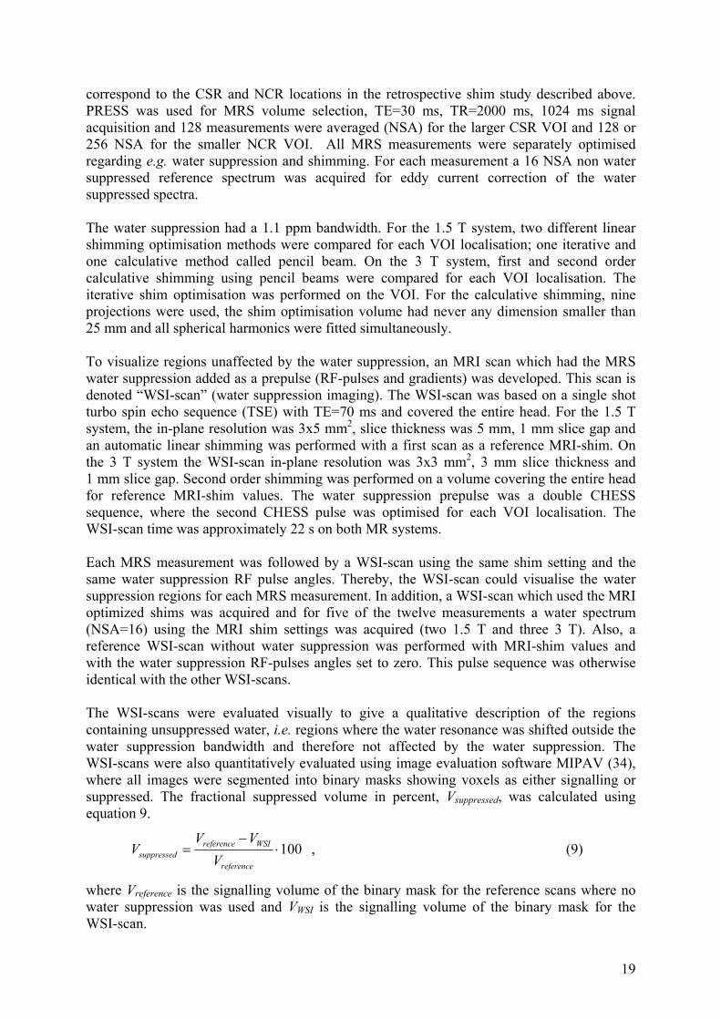
MRS phantom Two thin glass test tubes (175 mm long; 4 mm inner diameter; NMR sample tubes, (Wilmad Glass, USA) filled with the liquid sample were positioned horizontally in a head coil. The tubes were arranged perpendicularly to each other, one parallel and one transversal to the static magnetic field, B0. MRI phantom The phantom used for MRI was a 290 mm long coaxial circular cylinder (Fig. 11). It consists of an outer glass cylinder (compartment 4, 70.5 mm inner diameter) for the reference liquid (compartment 3) and an inner rod for a solid sample (compartments 1 and 2, 20.0 mm diameter) or an inner glass cylinder (compartment 2, 17.1 mm inner and 20.0 mm outer diameter) for a liquid sample or air (compartment 1). Distilled water (χV = -9.03 ppm at 20°C) was used as reference liquid. In total, 18 samples were imaged: 15 solutions with variable CuSO4 concentrations (6–400 mM; pro-analysis, CuSO4*5 H2O, Merck, Germany), 2 solid samples (PMMA and polyethylene) and air. MR systems Two MR systems, Philips Intera (1.5 T) and Philips ACS (1.5 T) (Philips Healthcare, The Netherlands), were used for non-volume selective MRS (1500 Hz bandwidth and 4096 samples) in the T/R head coil. Before MRS measurements, the systems were thoroughly shimmed using a spherical phantom (15 cm diameter) filled with doped saline solution.

Figure 11. A) The phantom used for MRI in the head coil. B) Cross section of the phantom. Outer cylinder (4) for reference liquid (3): 70.5 mm inner diameter; central sample: solid rod (1 and 2) 20.0 mm diameter or glass tube (2) 20.0 mm outer and 17.1 mm inner diameter filled with liquid sample (1). C) Simulation of a distortion. d is the distance between the intensity spots that appear due to signal elements positioned close to each other by the affected spatial encoding and reconstruction.

20

MRI was performed on a 1.5 T Magnetom Vision Plus software version VB33D and using the standard T/R head coil (Siemens AG, Germany). Before measurements, the system was thoroughly shimmed using a spherical phantom (180 millimetres diameter, containing 1000 g distilled water and 1.25 g NiSO4*6 H2O). The SE sequence had a gradient strength of 2.44 mT/m, providing a bandwidth of 104 kHz/m in the readout direction. The imaging parameters were as follows: FOV, 150 mm; matrix size, 256x256; TR, 300 ms; and TE, 35 ms. Five transaxial images with 10 mm slice thickness were acquired as cross sections of the phantom, and 6 of the 18 samples were measured with a CuSO4 concentration in the range of 12–400 mM. Samples with lower CuSO4 concentrations would not produce an artifact in the SE images. The EPI sequence was a SE–EPI and had a constant phase encoding gradient strength of 0.080 mT/m (corresponding to a bandwidth of 3.41 kHz/m), a frequency encoding gradient strength of 25 mT/m and a 75% partial scan. The imaging parameters used were the following: FOV, 245 mm; matrix size, 256x256; profile time, 1.2 ms; and TE, 137 ms. With EPI, 13 or 19 transaxial images with 10 mm slice thickness were acquired in all 18 samples.

3.2.2 Analysis The susceptibility of the CuSO4 solutions can be calculated theoretically from the CuSO4 concentration (30) and these susceptibility values were compared with both the MRI and MRS measurements. The images were evaluated using two different methods, one manual and one automatic in-house designed method based on model fitting.

MRS analysis The spectra were evaluated using jMRUI (35). The centre frequencies of the fitted Lorentzian curves were used in equation 10 to calculate the susceptibility of the sample.

( ) ioII χχδδ −=−⋅ ⊥2 , (10)

where χi is the susceptibility of the liquid inside the tubes and χo is the susceptibility for the medium outside the tubes, both given as parts per million. In paper IV, χo was denoted χe. δ⊥ and δII are the shift in reference frequency in ppm for the tube placed perpendicular and parallel to the magnetic field respectively (30).

MRI - manual image analysis The images were evaluated using the software Matlab 6.5 (Math Works, Natick, USA). The locations of the image intensity spots were determined by making three regions of interest (ROIs), one over each intensity spot, and by locating the pixel with the highest signal in each ROI. Equations 11a–11b (13) were then used to calculate the susceptibility of the sample.

2

2

1

232

30

3

22

1 )(829.2

2 χχχχ +⎟⎟⎠

⎞⎜⎜⎝

⎛⋅

⎥⎥⎦

⎤

⎢⎢⎣

⎡−−⎟

⎠⎞

⎜⎝⎛±=

aa

BGd

ar if d ≥ 2.305a2 (11a)

2

2

1

232

30

21 )(

707.1383.12 χχχχ +⎟⎟

⎠

⎞⎜⎜⎝

⎛⋅⎥

⎦

⎤⎢⎣

⎡−−⎟

⎠⎞

⎜⎝⎛ −

±=aa

BGad r if d ≤ 2.236a2 (11b)

where χn is the volume susceptibility and an is the outer radius for compartment n (Fig. 11b).

053

30 21 BB ⋅⎥⎦

⎤⎢⎣⎡ +

+=χχ (12)

B30 is the magnetic field in compartment 3 in an infinitely long coaxial cylinder, far from the interface between compartment 2 and 3 in which there is no effect from the susceptibility of

21

the sample (compartment 1). Gr is the gradient strength, and the artifact length, d, is defined as the distance between top and bottom intensity spots (Fig. 11c).

MRI - image analysis by model fitting An automatic and user independent evaluation program based on model fitting and iteration was developed. The susceptibility disturbance on the spatial encoding and the resulting misplacement, z’–z, of the signal were calculated using equation 13 (37). A simulated artifact was constructed by adding signals with the same image position. The simulated image was geometrically fitted to the MR image. By iteration, the susceptibility was found when the sum of absolute differences between pixel values of the model and the experiment was minimized.

)(' 22

2232 yz

yzaczz+−

⋅⋅=− where r

3032

2232

2121

GB

aa)(a)(

21c

⎭⎬⎫

⎩⎨⎧ χ−χ+χ−χ

= (13)

and z and y are the coordinates.

22

4. Results

4.1 The Spurious Echo Artifact (paper I, II and III)

4.1.1 k-space concept and simulations (paper I and II) Using the k-space concept it was possible to visualise how the unwanted magnetic configurations were shifted to different positions in k-space, while the signal from the VOI always ended up in the origin at the completion of volume selection. The spoiling of the model PRESS and STEAM sequences shifted the unwanted magnetic configurations to different positions in k-space, ranging from 500 m-1 to 5000-7000 m-1 in distance from the signal collection at the origin, depending on spoiling strengths chosen. Signal from magnetic configurations that are closest to the origin are most likely to refocus. In most variants of the model sequences, both for PRESS and STEAM, this was Mα3. The extension of an unwanted magnetic configuration determines the minimum distance that the configuration must be shifted away from the k-space origin, to avoid contributing signal to the spectrum. The slice profiles and their corresponding frequency spectra, i.e. their extension in k-space, are shown in figure 12. The simulated frequency spectra of the 3 cm slice profiles were 1/3 in width in comparison with the spectra of the 1 cm profiles. This reverse relationship between slice thickness and k-space extension is a fundamental property of Fourier space. When combining the PRESS k-space pattern of the spoiled magnetic configurations with the frequency spectra of the corresponding slice profiles, the frequency spread at the 10-5 level of the unwanted configurations was small compared to their distance from the origin for the 30x30x30 mm3 VOI. With a VOI of 10x10x10 mm3, the frequency spread at the 10-5 level (unsuppressed water signal) was comparable to the distance from origin for the closest of the unwanted configurations (Fig. 13), while the frequency spread was negligible for all configurations at the 10-1 level (metabolite signals). With twice as strong spoiling, the unwanted configurations were shifted to twice the distance from the origin. Altering the direction of the spoiling gradients in PRESS, the magnetic configurations were placed in three typical spoiling patterns (Fig. 14). The three spoiling patterns exist in four permutations through successive 90° rotations as well as four line-mirrored versions for the third pattern. When both spoiler pairs had the same direction (Fig. 14a) all magnetic configurations lined up, which only left two directions for refocusing any signal, and MSTE

was unfortunately left at the origin. This was avoided when the spoiler pairs differed in magnitude or direction, e.g. spoiler gradients applied perpendicular (Fig. 14c) which provided equal or less spoiling for all magnetic configurations except for MSTE. When altering the direction and strength of the TM spoiling in STEAM, the magnetic configurations were grouped into three groups. Group 1: Mα1, Mα2 and Mα1α2. Group 2: Mα1α3, Mα2α3, and Mα1α2α3. Group 3: MSTE, Mα3 and MSTE*. By increasing the TM spoiling strength, the distance between these groups was increased whereas the intra group distance was constant. Changing the direction of the TM spoiler the grouping of the magnetic configurations was the same and the first and second group was rotated by a change of the direction of the TM spoiling (Fig. 15c-f).

23

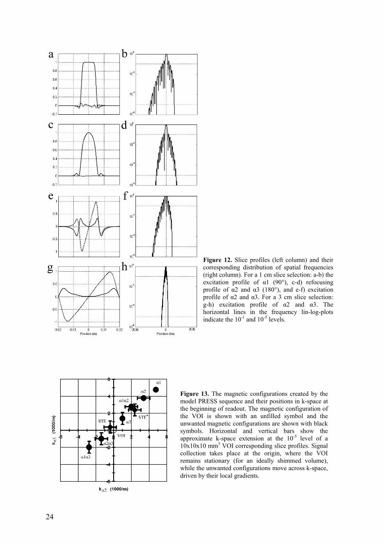
Figure 12. Slice profiles (left column) and their corresponding distribution of spatial frequencies (right column). For a 1 cm slice selection: a-b) the excitation profile of α1 (90°), c-d) refocusing profile of α2 and α3 (180°), and e-f) excitation profile of α2 and α3. For a 3 cm slice selection: g-h) excitation profile of α2 and α3. The horizontal lines in the frequency lin-log-plots indicate the 10-1 and 10-5 levels.

Figure 13. The magnetic configurations created by the model PRESS sequence and their positions in k-space at the beginning of readout. The magnetic configuration of the VOI is shown with an unfilled symbol and the unwanted magnetic configurations are shown with black symbols. Horizontal and vertical bars show the approximate k-space extension at the 10-5 level of a 10x10x10 mm3 VOI corresponding slice profiles. Signal collection takes place at the origin, where the VOI remains stationary (for an ideally shimmed volume), while the unwanted configurations move across k-space, driven by their local gradients.

24

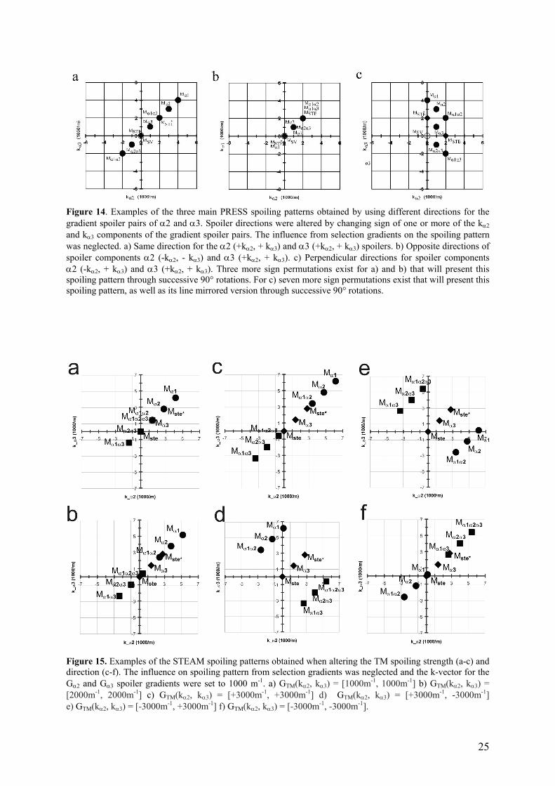
Figure 14. Examples of the three main PRESS spoiling patterns obtained by using different directions for the gradient spoiler pairs of α2 and α3. Spoiler directions were altered by changing sign of one or more of the kα2 and kα3 components of the gradient spoiler pairs. The influence from selection gradients on the spoiling pattern was neglected. a) Same direction for the α2 (+kα2, + kα3) and α3 (+kα2, + kα3) spoilers. b) Opposite directions of spoiler components α2 (-kα2, - kα3) and α3 (+kα2, + kα3). c) Perpendicular directions for spoiler components α2 (-kα2, + kα3) and α3 (+kα2, + kα3). Three more sign permutations exist for a) and b) that will present this spoiling pattern through successive 90° rotations. For c) seven more sign permutations exist that will present this spoiling pattern, as well as its line mirrored version through successive 90° rotations.

Figure 15. Examples of the STEAM spoiling patterns obtained when altering the TM spoiling strength (a-c) and direction (c-f). The influence on spoiling pattern from selection gradients was neglected and the k-vector for the Gα2 and Gα3 spoiler gradients were set to 1000 m-1. a) GTM(kα2, kα3) = [1000m-1, 1000m-1] b) GTM(kα2, kα3) = [2000m-1, 2000m-1] c) GTM(kα2, kα3) = [+3000m-1, +3000m-1] d) GTM(kα2, kα3) = [+3000m-1, -3000m-1] e) GTM(kα2, kα3) = [-3000m-1, +3000m-1] f) GTM(kα2, kα3) = [-3000m-1, -3000m-1].

25

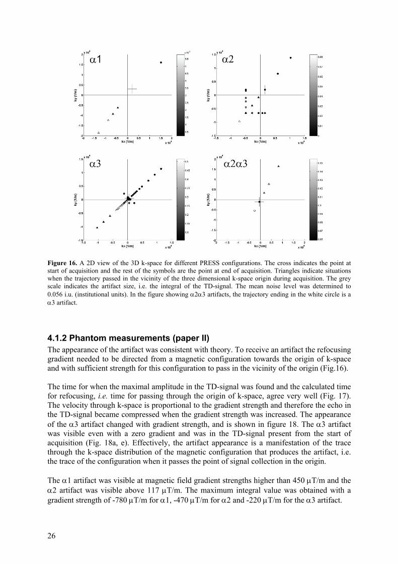
Figure 16. A 2D view of the 3D k-space for different PRESS configurations. The cross indicates the point at start of acquisition and the rest of the symbols are the point at end of acquisition. Triangles indicate situations when the trajectory passed in the vicinity of the three dimensional k-space origin during acquisition. The grey scale indicates the artifact size, i.e. the integral of the TD-signal. The mean noise level was determined to 0.056 i.u. (institutional units). In the figure showing α2α3 artifacts, the trajectory ending in the white circle is a α3 artifact.

4.1.2 Phantom measurements (paper II) The appearance of the artifact was consistent with theory. To receive an artifact the refocusing gradient needed to be directed from a magnetic configuration towards the origin of k-space and with sufficient strength for this configuration to pass in the vicinity of the origin (Fig.16). The time for when the maximal amplitude in the TD-signal was found and the calculated time for refocusing, i.e. time for passing through the origin of k-space, agree very well (Fig. 17). The velocity through k-space is proportional to the gradient strength and therefore the echo in the TD-signal became compressed when the gradient strength was increased. The appearance of the α3 artifact changed with gradient strength, and is shown in figure 18. The α3 artifact was visible even with a zero gradient and was in the TD-signal present from the start of acquisition (Fig. 18a, e). Effectively, the artifact appearance is a manifestation of the trace through the k-space distribution of the magnetic configuration that produces the artifact, i.e. the trace of the configuration when it passes the point of signal collection in the origin. The α1 artifact was visible at magnetic field gradient strengths higher than 450 μT/m and the α2 artifact was visible above 117 μT/m. The maximum integral value was obtained with a gradient strength of -780 μT/m for α1, -470 μT/m for α2 and -220 μT/m for the α3 artifact.

26

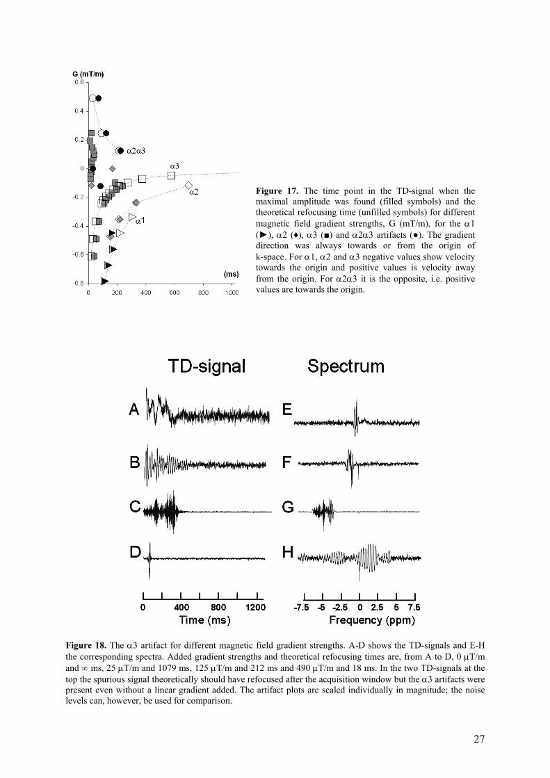
Figure 17. The time point in the TD-signal when the maximal amplitude was found (filled symbols) and the theoretical refocusing time (unfilled symbols) for different magnetic field gradient strengths, G (mT/m), for the α1 (►), α2 (♦), α3 (■) and α2α3 artifacts (●). The gradient direction was always towards or from the origin of k-space. For α1, α2 and α3 negative values show velocity towards the origin and positive values is velocity away from the origin. For α2α3 it is the opposite, i.e. positive values are towards the origin.

Figure 18. The α3 artifact for different magnetic field gradient strengths. A-D shows the TD-signals and E-H the corresponding spectra. Added gradient strengths and theoretical refocusing times are, from A to D, 0 μT/m and ∞ ms, 25 μT/m and 1079 ms, 125 μT/m and 212 ms and 490 μT/m and 18 ms. In the two TD-signals at the top the spurious signal theoretically should have refocused after the acquisition window but the α3 artifacts were present even without a linear gradient added. The artifact plots are scaled individually in magnitude; the noise levels can, however, be used for comparison.

27

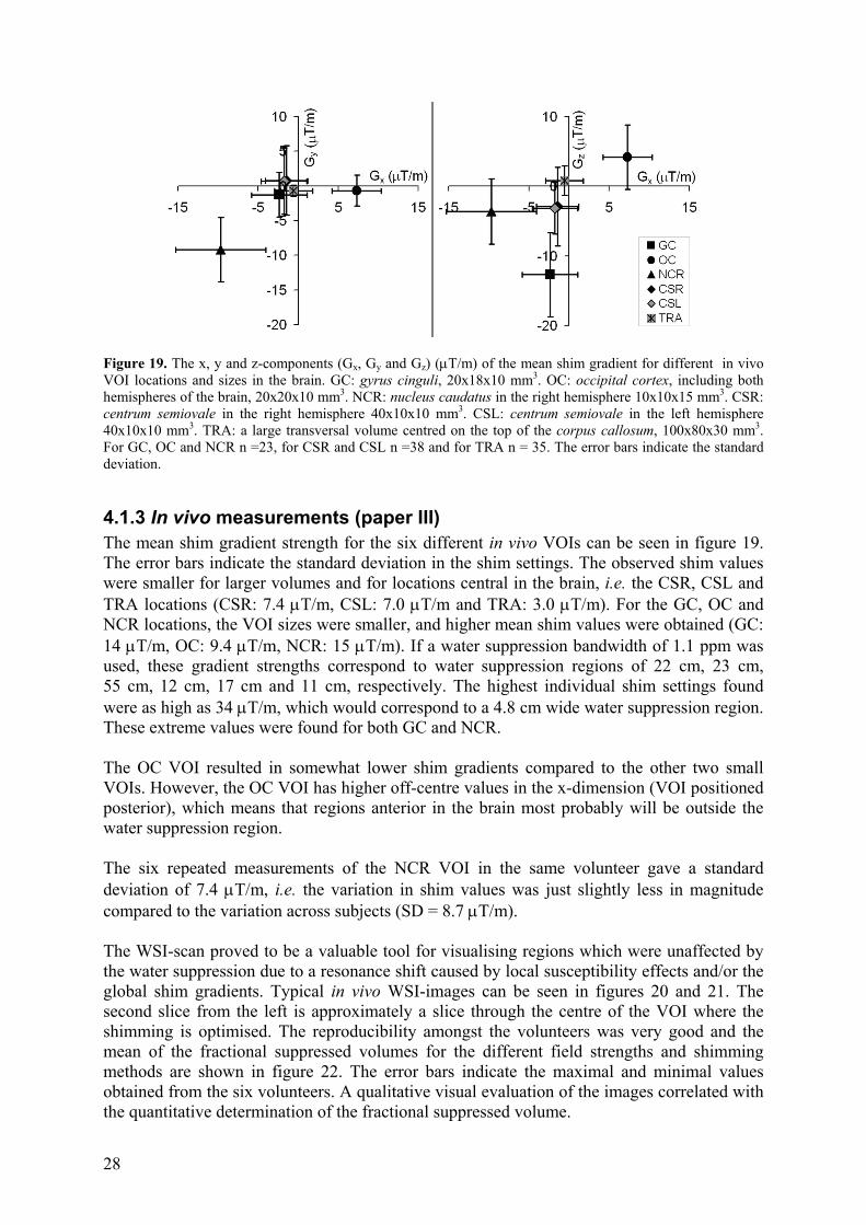
Figure 19. The x, y and z-components (Gx, Gy and Gz) (μT/m) of the mean shim gradient for different in vivo VOI locations and sizes in the brain. GC: gyrus cinguli, 20x18x10 mm3. OC: occipital cortex, including both hemispheres of the brain, 20x20x10 mm3. NCR: nucleus caudatus in the right hemisphere 10x10x15 mm3. CSR: centrum semiovale in the right hemisphere 40x10x10 mm3. CSL: centrum semiovale in the left hemisphere 40x10x10 mm3. TRA: a large transversal volume centred on the top of the corpus callosum, 100x80x30 mm3. For GC, OC and NCR n =23, for CSR and CSL n =38 and for TRA n = 35. The error bars indicate the standard deviation.

4.1.3 In vivo measurements (paper III) The mean shim gradient strength for the six different in vivo VOIs can be seen in figure 19. The error bars indicate the standard deviation in the shim settings. The observed shim values were smaller for larger volumes and for locations central in the brain, i.e. the CSR, CSL and TRA locations (CSR: 7.4 μT/m, CSL: 7.0 μT/m and TRA: 3.0 μT/m). For the GC, OC and NCR locations, the VOI sizes were smaller, and higher mean shim values were obtained (GC: 14 μT/m, OC: 9.4 μT/m, NCR: 15 μT/m). If a water suppression bandwidth of 1.1 ppm was used, these gradient strengths correspond to water suppression regions of 22 cm, 23 cm, 55 cm, 12 cm, 17 cm and 11 cm, respectively. The highest individual shim settings found were as high as 34 μT/m, which would correspond to a 4.8 cm wide water suppression region. These extreme values were found for both GC and NCR. The OC VOI resulted in somewhat lower shim gradients compared to the other two small VOIs. However, the OC VOI has higher off-centre values in the x-dimension (VOI positioned posterior), which means that regions anterior in the brain most probably will be outside the water suppression region. The six repeated measurements of the NCR VOI in the same volunteer gave a standard deviation of 7.4 μT/m, i.e. the variation in shim values was just slightly less in magnitude compared to the variation across subjects (SD = 8.7 μT/m). The WSI-scan proved to be a valuable tool for visualising regions which were unaffected by the water suppression due to a resonance shift caused by local susceptibility effects and/or the global shim gradients. Typical in vivo WSI-images can be seen in figures 20 and 21. The second slice from the left is approximately a slice through the centre of the VOI where the shimming is optimised. The reproducibility amongst the volunteers was very good and the mean of the fractional suppressed volumes for the different field strengths and shimming methods are shown in figure 22. The error bars indicate the maximal and minimal values obtained from the six volunteers. A qualitative visual evaluation of the images correlated with the quantitative determination of the fractional suppressed volume.

28

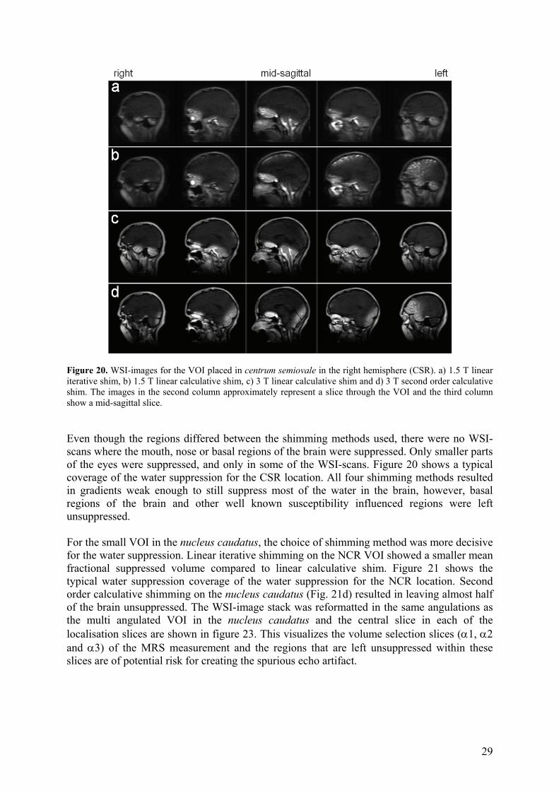
Figure 20. WSI-images for the VOI placed in centrum semiovale in the right hemisphere (CSR). a) 1.5 T linear iterative shim, b) 1.5 T linear calculative shim, c) 3 T linear calculative shim and d) 3 T second order calculative shim. The images in the second column approximately represent a slice through the VOI and the third column show a mid-sagittal slice. Even though the regions differed between the shimming methods used, there were no WSI-scans where the mouth, nose or basal regions of the brain were suppressed. Only smaller parts of the eyes were suppressed, and only in some of the WSI-scans. Figure 20 shows a typical coverage of the water suppression for the CSR location. All four shimming methods resulted in gradients weak enough to still suppress most of the water in the brain, however, basal regions of the brain and other well known susceptibility influenced regions were left unsuppressed. For the small VOI in the nucleus caudatus, the choice of shimming method was more decisive for the water suppression. Linear iterative shimming on the NCR VOI showed a smaller mean fractional suppressed volume compared to linear calculative shim. Figure 21 shows the typical water suppression coverage of the water suppression for the NCR location. Second order calculative shimming on the nucleus caudatus (Fig. 21d) resulted in leaving almost half of the brain unsuppressed. The WSI-image stack was reformatted in the same angulations as the multi angulated VOI in the nucleus caudatus and the central slice in each of the localisation slices are shown in figure 23. This visualizes the volume selection slices (α1, α2 and α3) of the MRS measurement and the regions that are left unsuppressed within these slices are of potential risk for creating the spurious echo artifact.

29

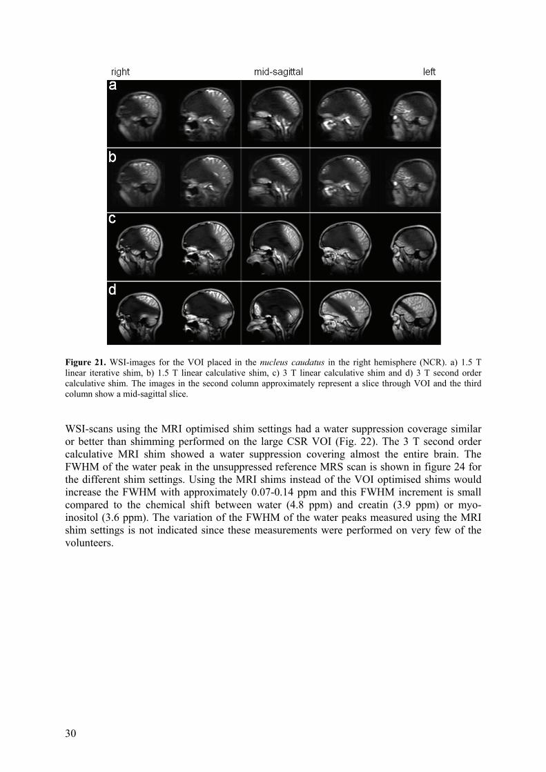
Figure 21. WSI-images for the VOI placed in the nucleus caudatus in the right hemisphere (NCR). a) 1.5 T linear iterative shim, b) 1.5 T linear calculative shim, c) 3 T linear calculative shim and d) 3 T second order calculative shim. The images in the second column approximately represent a slice through VOI and the third column show a mid-sagittal slice. WSI-scans using the MRI optimised shim settings had a water suppression coverage similar or better than shimming performed on the large CSR VOI (Fig. 22). The 3 T second order calculative MRI shim showed a water suppression covering almost the entire brain. The FWHM of the water peak in the unsuppressed reference MRS scan is shown in figure 24 for the different shim settings. Using the MRI shims instead of the VOI optimised shims would increase the FWHM with approximately 0.07-0.14 ppm and this FWHM increment is small compared to the chemical shift between water (4.8 ppm) and creatin (3.9 ppm) or myo-inositol (3.6 ppm). The variation of the FWHM of the water peaks measured using the MRI shim settings is not indicated since these measurements were performed on very few of the volunteers.

30

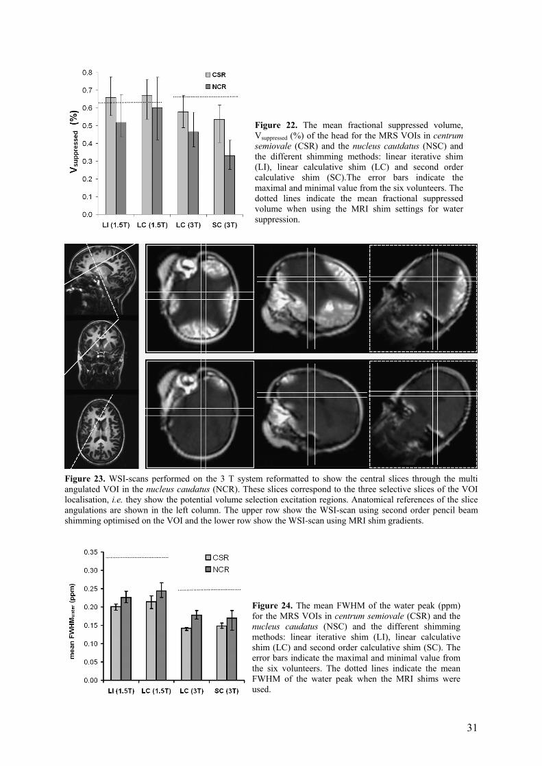
Figure 22. The mean fractional suppressed volume, Vsuppressed (%) of the head for the MRS VOIs in centrum semiovale (CSR) and the nucleus cautdatus (NSC) and the different shimming methods: linear iterative shim (LI), linear calculative shim (LC) and second order calculative shim (SC).The error bars indicate the maximal and minimal value from the six volunteers. The dotted lines indicate the mean fractional suppressed volume when using the MRI shim settings for water suppression.

Figure 23. WSI-scans performed on the 3 T system reformatted to show the central slices through the multi angulated VOI in the nucleus caudatus (NCR). These slices correspond to the three selective slices of the VOI localisation, i.e. they show the potential volume selection excitation regions. Anatomical references of the slice angulations are shown in the left column. The upper row show the WSI-scan using second order pencil beam shimming optimised on the VOI and the lower row show the WSI-scan using MRI shim gradients.

Figure 24. The mean FWHM of the water peak (ppm) for the MRS VOIs in centrum semiovale (CSR) and the nucleus caudatus (NSC) and the different shimming methods: linear iterative shim (LI), linear calculative shim (LC) and second order calculative shim (SC). The error bars indicate the maximal and minimal value from the six volunteers. The dotted lines indicate the mean FWHM of the water peak when the MRI shims were used.

31

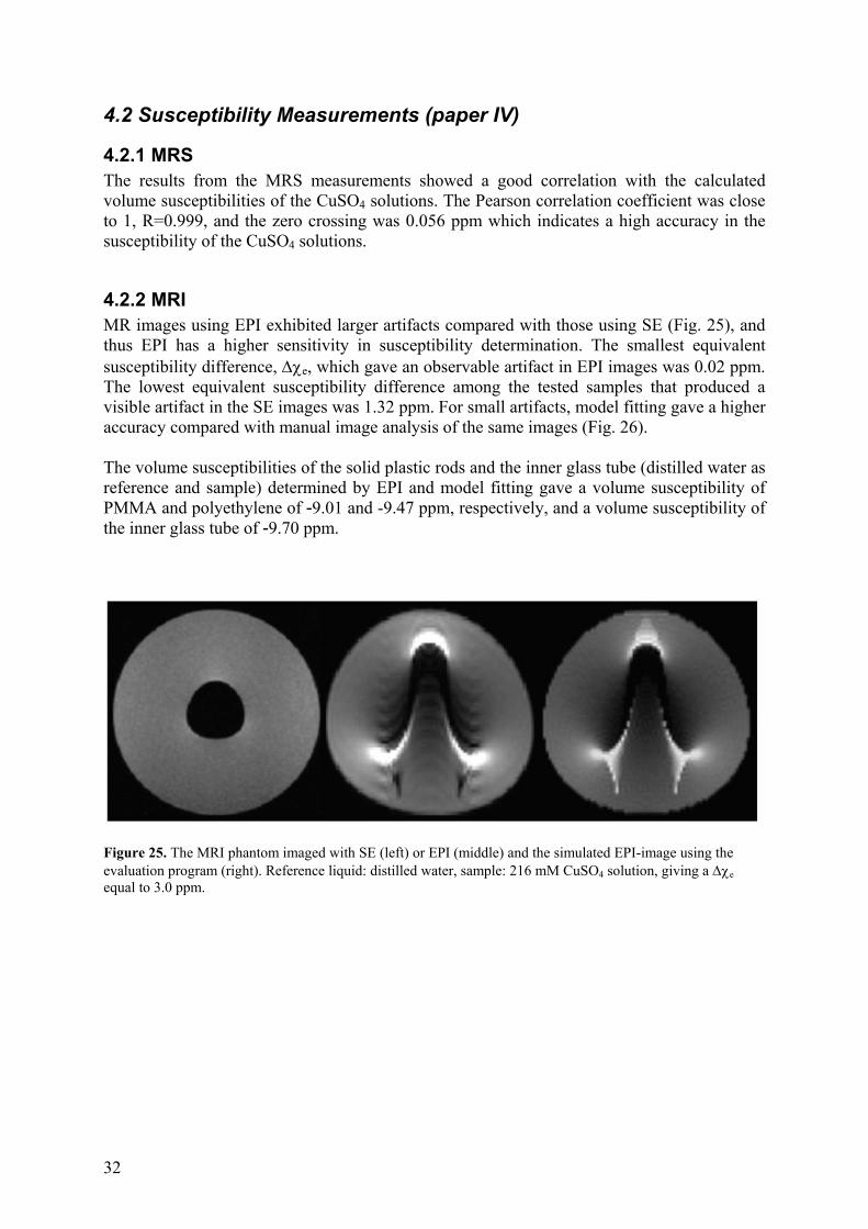
4.2 Susceptibility Measurements (paper IV)

4.2.1 MRS The results from the MRS measurements showed a good correlation with the calculated volume susceptibilities of the CuSO4 solutions. The Pearson correlation coefficient was close to 1, R=0.999, and the zero crossing was 0.056 ppm which indicates a high accuracy in the susceptibility of the CuSO4 solutions.

4.2.2 MRI MR images using EPI exhibited larger artifacts compared with those using SE (Fig. 25), and thus EPI has a higher sensitivity in susceptibility determination. The smallest equivalent susceptibility difference, Δχe, which gave an observable artifact in EPI images was 0.02 ppm. The lowest equivalent susceptibility difference among the tested samples that produced a visible artifact in the SE images was 1.32 ppm. For small artifacts, model fitting gave a higher accuracy compared with manual image analysis of the same images (Fig. 26). The volume susceptibilities of the solid plastic rods and the inner glass tube (distilled water as reference and sample) determined by EPI and model fitting gave a volume susceptibility of PMMA and polyethylene of -9.01 and -9.47 ppm, respectively, and a volume susceptibility of the inner glass tube of -9.70 ppm.

Figure 25. The MRI phantom imaged with SE (left) or EPI (middle) and the simulated EPI-image using the evaluation program (right). Reference liquid: distilled water, sample: 216 mM CuSO4 solution, giving a Δχe equal to 3.0 ppm.

32

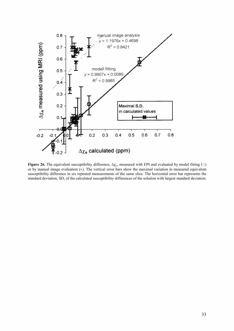
Figure 26. The equivalent susceptibility difference, Δχe, measured with EPI and evaluated by model fitting ( ) or by manual image evaluation (×). The vertical error bars show the maximal variation in measured equivalent susceptibility difference in six repeated measurements of the same slice. The horizontal error bar represents the standard deviation, SD, of the calculated susceptibility differences of the solution with largest standard deviation.

33

34

5. Discussion The trend in clinical MR is towards higher magnetic field strengths, from 1.5 T to 3 T and beyond. Increasing the magnetic field strength leads to increased susceptibility effects, both in MRI and MRS. To be able to have control of your phantom studies, you need to have control of the susceptibilities and susceptibility effects in your measurements. The susceptibility differences of phantoms used in different studies might give a pronounced effect on your measurement result and therefore it is valuable to have an easy and accessible method to measure the volume susceptibility with the MR system. The increased magnetic field strength also leads to increased SNR (signal to noise ratio), and hence, smaller VOIs become more accessible in MRS. The smaller VOIs are often preferred as they enable MRS measurements that are well focused on specific regions and also increases the possibility of achieving a good local shim within the VOI (38). However, the global effects of the locally optimised shim gradients might cause regions where the water resonance is shifted outside the water suppression bandwidth. When these regions are large, they are more probable to overlap with the volume selection excitation regions and hence the probability of a spurious echo artifact increases. Based on the concept of trajectories in k-space, it was possible to show all the different positions of the nine magnetic configurations prior to signal acquisition in one single k-space map. This k-space description was verified with in vitro measurements and this tool proved to be very powerful when describing the effective spoiling of unwanted magnetic configurations. To some extent, the k-space concept could also be used to describe how local gradients may drive the configurations differently during acquisition.

5.1 The Spurious Echo Artifact (paper I, II and III) A VOI which is well shimmed during volume selection and signal acquisition gives more narrow peaks, i.e. a higher spectral resolution. Many interesting parts of the brain have, in general, been inaccessible to MRS due to severe local magnetic field inhomogeneities. Basal and frontal areas are examples of such regions that might, to some extent, become accessible with smaller VOIs and more advanced shimming methods (38,39). If the VOI is well shimmed during water suppression, the water signal in the VOI can be well suppressed without the risk of affecting any of the metabolites close to water. However, successful cancellation of a large local magnetic field gradient in the VOI transforms, via the shim gradient, this large local gradient to a global one, which will affect and shift the resonance frequencies of the object within the coil sensitivity volume. Hence, water resonances outside the VOI might be shifted outside the water suppression band. The effects of shimming on the in vivo water suppression performance have, to my knowledge, not previously been studied. However, an in vitro experiment which confirms that locally optimised shimming can cause unsuppressed outer volume water signal has previously been performed (40). The WSI-scan presented in paper III appeared to be a valuable tool for visualising regions in vivo that were unaffected by the water suppression. It was possible to visually evaluate the combined effects of the global shim gradients and any local susceptibility induced magnetic fields.

35

The shim gradient can only balance the mean gradient of the same order in the VOI, e.g. the linear shim can only balance the mean linear gradient of the local magnetic field over the VOI. Therefore, in a small VOI, more local inhomogeneities can be balanced, and hence, higher shim values become more probable. The smaller VOIs did show higher shim values and large regions of unsuppressed water (Figs. 19 and 22). The complex patterns of the water suppressed regions appeared very similar for all six volunteers and unexpectedly the standard deviation of the linear shim values was of the same magnitude for the 23 volunteers as for the six repeated measurements in the same volunteer. However, the nucleus caudatus was chosen as a localisation known to be influenced by susceptibility effects (41) and a small shift of the VOI, relative to the anatomy, probably affects the magnetic field over the VOI in the same magnitude as the variation across subjects. As suspected, the larger VOIs showed lower shim values and larger water suppression regions in both the retrospective shim value study and in the study using WSI-scans. For the larger VOI, there were no large differences between the shim optimisation methods, or between first and second order shimming. Using second order shimming for the nucleus caudatus, the water suppression only covered about 35% of the head. Using linear shimming, larger regions of the brain were covered but there were still regions, mostly occipital or basal regions of the brain, where the water signal was left unsuppressed. Compared to linear calculative shim, linear iterative shimming on the NCR VOI showed a smaller mean fractional suppressed volume. The optimisation of the calculative shim was forced to use a shim volume with dimensions equal to or larger than 25 mm whereas the iterative shim was performed on the actual MRS VOI, i.e. 10x10x15 mm3. The iterative shim was thus optimised for a spatially smaller local magnetic field, which explains a higher shim gradient and also a smaller water suppression region. Hence, the difference in fractional suppressed volume is probably not caused by the difference in optimisation method but by the different sizes of the optimisation volumes. VOIs positioned off-centre will cause larger regions to be left unsuppressed since the spatial centrum for water suppression is shifted with the VOI. For a VOI positioned off-centre, a second order shim gradient will also force the use of a linear gradient to balance the linear component of the second order gradient in VOI (11). This added linear gradient will only balance the linear component of the second order gradient inside the VOI, while globally it will add to the second order gradient and can thereby cause large magnetic field gradients. Hence, using higher order shimming on small VOIs, and especially, small VOIs positioned off-centre, will cause significant and complex magnetic field gradients outside the VOI. Paper III showed that when performing small VOI 1H MRS, the shim gradients will degrade the water suppression. Even though the size of the regions differed between the large and small VOI, there were no WSI-scans where the mouth, nose or basal regions of the brain were suppressed. Only smaller parts of the eyes were suppressed, and only in some of the WSI-scans. When the regions of non-suppressed water overlap with the excitation regions of the volume selection, they become sources for potential spurious echo artifacts. The volume selection excitation regions differ for the different volume selection methods. STEAM consists of three 90° excitation slices whereas PRESS consists of one 90° excitation slice and two 180° refocusing slices. However, all three-pulse experiments are capable of forming the same nine magnetic configurations (19-21). The relative amplitude, the spatial

36

regions and the regions in k-space corresponding to these configurations will differ and depend on the pulses in the volume selection. In the k-space concept (12) all gradients and RF-pulses of the volume selection sequence affects the k-space trajectories for the magnetic configurations. The strong spoiling gradients shifted the unwanted magnetic configurations away from the origin of k-space, i.e. the point of signal collection. Changing the spoiling gradient strength and/or direction can thereby be a powerful tool for eliminating spurious echoes. The possibilities to distribute the unwanted configurations in k-space were different for PRESS and STEAM. For example, in STEAM the mixing time spoiler could be used to increase the spoiling of six of the configurations without increasing the echo time. However, the α3 configuration will not be affected by the mixing time spoiling. In paper I simulations of realistic slice profiles and their corresponding frequency spectra were performed. The range of spatial frequencies with amplitudes above the 10-5 level represents the extension in k-space of unsuppressed water signal from the slice that can not be neglected if it contributes to the MR spectrum. For a 1 cm slice the extensions were about 1500 m-1 and this indicates that a spoiling power of about 1000 m-1 would be sufficient, assuming a perfect homogeneous magnetic filed over the entire object. The k-space trajectory will be affected by all magnetic field gradients present over the excitation regions. During volume selection local magnetic field gradients and shim gradients are probably negligible compared to the stronger selection and spoiling gradients applied in the volume selection pulse sequence. However, during the long signal acquisition even small local gradients may cause a significant continuation of the k-space trajectory. Shimming the VOI prevents the magnetic configuration of the VOI from drifting off the k-space origin during signal acquisition. The course of the other configurations is determined by the B0 field variation resulting over the respective excitation region. Susceptibility induced local gradients together with the global effect of the shimming gradients can cause some of the configurations to pass the origin, or in its vicinity, i.e. cause a refocusing. Moonen et al. theoretically established that a local magnetic field gradient might act as a refocusing gradient (27), but, the influence of the global shim gradient was not included. The position at start of signal acquisition, in terms of both distance and direction relative to the k-space origin, is the prerequisite to prevent an unwanted magnetic configuration from refocusing. When combining the extension of the magnetic configuration in k-space for unsuppressed water and a small VOI with the spoiling pattern (Fig. 13) it is obvious that those configurations that are positioned closest to the origin pose a considerable risk of unwanted contribution in the collection of signal. The k-space coverage for these configurations is so large that they can hardly miss the origin, should they drift at all towards it. The results demonstrate that a gradient spoiling sufficient for elimination of unwanted signal for a given VOI size may not be sufficient for a smaller one. Likewise, a gradient spoiling that is sufficient for elimination of unwanted metabolite signal may not be sufficient for elimination of unsuppressed water signal. Hence, it is unlikely that there exists any fixed spoiling scheme that is optimal for all in vivo measurement situations. Rather, the spoiling has to be tailored for each measurement to eliminate the probability of spurious signal. The simulations and the k-space description of spurious echoes provide a basic theoretical tool for analysis of spoiling schemes and prediction of spurious signal.

37

The k-space description was verified by in vitro experiments and the appearance of the artifact was consistent with theory. To receive an artifact the refocusing gradient needed to be directed from a magnetic configuration towards the origin of k-space, and with sufficient strength for at least parts of the k-space distribution of the configuration to pass in the vicinity of the origin (Fig. 16). The gradient strength will determine the velocity by which the magnetic configuration passes the k-space origin and therefore the echo in the TD-signal became compressed when the gradient strength was increased. The trace through the k-space distribution of the magnetic configuration that passes through the point of signal collection will be decisive for the artifact appearance. The smaller artifacts appeared similar to the one published by Kreis (28), but differed somewhat from the ones published by Ernst et al. (26) which had less structure and were not as limited in frequency range. Papers I-III have clearly shown that for small VOI 1H MRS there are large regions of unsuppressed water, which most likely will overlap with the volume selection excitation regions, and that since the time for signal acquisition is much longer than the time for volume selection any refocusing gradient can be much weaker than the spoiling gradients and still refocus unwanted magnetic configurations into spurious echoes. As a result, there will only be the phase cycling left to prohibit the formation of a spurious echo artifact in the acquired spectrum. Henning illustrated how the phase cycling scheme called phase rotation effectively can cancel the spurious echoes (42). However, at this stage, a successful measurement relies on acquisitions from a number of phase cycles, each one contaminated with spurious signal, which when accumulated over all phase cycles cancels the spurious signal leaving an artifact free spectrum. PRESS and STEAM, which commonly are regarded as single experiment volume selection methods have turned into multi experiment methods and, as such, they are sensitive to object motion. The WSI-scans showed that regions which always were left unaffected by the water suppression were the mouth, nose and basal regions of the brain. These regions are also suffering from tissue motion and hence are regions where the phase cycling is more probable to fail. Almost all water suppression methods used are based on the chemical shift between water and the other resonances and all methods based on frequency selective excitation will be affected by the shim gradients. Increasing the number of CHESS pulses and implementing more efficient water suppression methods, e.g. DRYSTEAM (43), will not change the water suppression regions, and the regions will probably be very similar to what was shown in paper III. All these water suppression methods might benefit from using a more global shim for the water suppression. The actual volume selection and signal acquisition must be performed using the locally optimised shim to ensure a high spectral resolution. However, by choosing a more global shim, e.g. the imaging shim, during the water suppression part of the MRS measurement, a good coverage of the water suppression can be obtained. Due to the difference in resonance frequency between the two different shim settings, there is a risk of suppressing metabolite signal with the water suppression RF-pulses. In the present work, FWHM of the water peak showed a slight increase when the MRI shim was used, compared to when the VOI-optimised shim was used. In this thesis several ways to improve 1H MRS measurements by reducing the risk of a spurious echo artifact have been identified. For example, better prerequisites for MRS could be accomplished by implementing the WSI-scan in the MRS preparation. The WSI-scan used in this work was quick (22 s) and could easily be used for routine clinical MRS measurements. The WSI-images can then be used to adjust the slice order so that the α3 slice does not overlap with regions of unsuppressed water and tissue motion. Previous studies have

38

recommended an optimal slice order, placing the α3 slice in a transversal direction (26,27). With today’s use of multi angulated VOIs this recommendation needs to be updated. For multi angulated VOIs, and due to the complexity caused by higher order shim gradients, it will be very difficult to determine an optimal slice order without the information of the actual water suppression regions. An alternative approach can be to use the WSI-scan to indicate where to place saturation bands for extra outer volume suppression. The capability of the volume selection sequences to suppress spurious signal could be improved by increasing the spoiler gradients. The strength of the gradient will be limited by available gradient power and the durations will be limited by TE. Larger spoiler gradients might also lead to more eddy currents in the scanner and an increased risk of phase errors due to motion during the application of a spoiler gradient pair (44). Another option is to alter the directions of the spoiler gradients. This will be the equivalent to repositioning the spoiled configurations in k-space. Since the purpose is to avoid or remedy refocusing of spurious signal in each measurement situation, selection of spoiling directions should be guided by the direction of the shim gradient (Fig. 8). If it is not possible to change the sequence implementation there are several simple ways to try to eliminate the spurious echo artifact. First, immobilise the patient to prevent motion, e.g. using a vacuum cushion. Second, use as large VOI as possible, since the larger VOIs reduce the shim gradient strengths and reduce the extension of the signal region in k-space. Third, use linear shims for small VOIs, since the spectral resolution often is high enough even with first order shims. If second order is needed, the dimensions of the shim volume should be increased. Fourth, try to angulate the VOI so the extensions of the volume selection slices do not cross regions containing tissue motion. If this is hard to achieve, try using a saturation band. Finally, it is advisable to always study the FID and spectrum during signal acquisition. If a spurious echo artifact does turn up in the first measurements, it is advisable to abort the acquisition, change the slice order, reangulate or move the VOI slightly and restart the measurement. This thesis describes and discusses spurious signal in the context of 1H MRS in the brain. However, the theoretical considerations and the results are, in principle, valid for application of 1H MRS in any other part of the living body.

5.2 Susceptibility Measurements (paper IV) The MRS method for susceptibility measurements (30) was easy to use and is accurate, and there was no need for large sample sizes or well-known references other than air. However, due to broad peaks overlapping each other for samples with short T2 relaxation times, the MRS method is only suitable for liquids with sufficiently long T2 values. Other liquids, and all solids, require the MRI method. The MRI method was first implemented using a SE sequence (13). However, using EPI and model fitting for evaluation proved to be comparable with the MRS method with regard to accuracy and sensitivity. In the measurements using the EPI sequence the limit for an observable artifact was Δχe =0.02 ppm (as compared to 0.01 ppm for the MRS method). When considering the relative bandwidth per meter for the readout gradient in the SE sequence, compared with that of the phase encoding gradient in the EPI sequence, the

39

sensitivity was increased by a factor of 30 using EPI. With such a high increase in sensitivity, it would be possible to measure much smaller sample sizes, theoretically 5.5 times thinner, and still get the same artifact size, but the spatial resolution and SNR will be restricting factors. The ultimate limitation of susceptibility determination with MRI is, however, set by the field inhomogeneities remaining after shimming, i.e. it is of outmost importance that the shimming of the MR system is thorough and that there are prerequisites for a good shim. Model fitting was found to be superior to the manual image analysis because it utilised the entire artifact instead of only the three intensity spots as in the original evaluation method (13). This will make the evaluation and susceptibility determination less sensitive to other image artifacts. It also made it possible to accurately evaluate smaller susceptibility artifacts, e.g. images with only a barely visible artifact could be evaluated with a satisfying result. Being able to perform susceptibility measurements of plastics using distilled water as a reference makes it easy and accessible for everyone to perform susceptibility determination for phantom materials with an MR system. Model fitting should be used for evaluation if very high accuracy is needed in the susceptibility measurements. However, for many applications the manual analysis is probably good enough if the sensitivity in the imaging is high.

40

6. Conclusion In this thesis the susceptibility effects in MRI and 1H MRS were studied. Using the well recognised, but often unwanted, effects of susceptibility in EPI imaging the sensitivity of susceptibility measurements could be greatly improved. In MRS, susceptibility is well known to cause line broadening; however, the role of susceptibility in the creation of spurious echo artifacts is unknown to many. In this thesis the origin of the spurious echo artifact was explored using a k-space concept. One single k-space map could show all the different magnetic configurations and their relative positions. It was easy to follow the magnetic configurations during volume selection and to see the effective spoiling power prior to signal acquisition. To some extent the k-space description could also be used to describe the continuing trajectory during signal acquisition, and any refocusing of spurious echoes. The k-space description of the artifact was verified by in vitro measurements. Different magnetic configurations of the PRESS sequence were separately refocused using linear magnetic field gradients. The artifact appearance was consistent with theory. The in vitro measurements showed that the characteristics of the artifact strongly depended on the strength of the refocusing gradient. In the time domain signal the artifact is an imprint of the magnetic configuration as it passed through the origin of k-space during signal acquisition. The k-space concept provided a geometrical approach that proved to be especially valuable for discussing spoiling strategies. The position of the magnetic configurations at the start of acquisition, in terms of both distance and direction relative to the k-space origin, was a prerequisite to prevent refocusing of any of the configurations into a spurious echo. The k-space concept was applied on both STEAM and PRESS, where different spoiling patterns were examined. For STEAM it is possible to increase the spoiling power for six of the magnetic configurations, without affecting the shortest possible echo time which is not possible for PRESS. For both sequences the free induction decay of the last RF-pulse in the volume selection, α3, became the configuration closest to the k-space origin and was therefore the magnetic configuration most likely to cause a spurious echo artifact. However, for neither PRESS nor STEAM it was possible to increase the α3 spoiling without increasing the shortest possible echo time. This thesis showed how localised shimming in small VOIs can degrade the water suppression performance in 1H MRS. An imaging scan, the WSI-scan, was developed in which the MRS water suppression sequence was added as a pre-pulse. The accuracy of the WSI-scan was validated in vitro. In vivo the WSI-scan, with high contrast, visualised the regions unaffected by the water suppression, irrespective of if the shift in resonance frequency was caused by local susceptibility effects or the global shim gradients. For the large VOI in the homogeneous region of centrum semiovale, all shimming methods gave a similar result; the shim values were lower and the water signal was suppressed in most parts of the brain. For the small VOI in the more inhomogeneous magnetic field around nucleus caudatus, the choice of shimming method was more decisive for the water suppression performance. Second order shimming of the small VOI resulted in very large, complex regions of the brain where the water signal was left unsuppressed. Considering the small gain in FWHM of the water peak for second order shimming, second order shimming will most probably cause

41

more damage than gain for small VOIs. The quality of the small VOI 1H MRS measurements would most probably benefit if the water suppression shim was optimised on a more global volume and separated from the shim used during volume selection and signal acquisition. On a clinical MR scanner, the use of EPI instead of a standard implementation of an SE sequence increases the sensitivity in susceptibility measurements significantly. Increased sensitivity gives an opportunity to detect smaller susceptibility differences, to be more flexible in choice of reference liquid and to decrease the sample radius and volume. An automated evaluation method based on model fitting was developed, and evaluation by this method increased the accuracy further and the volume susceptibilities of two different plastics were determined. Being able to determine the susceptibility for phantom materials makes it possible to reduce unwanted susceptibility effects in phantom measurements. In summary, susceptibility is a common source for artifacts in both MRI and MRS and the importance of understanding susceptibility effects increases with field strength. The k-space concept, the WSI-scan and the susceptibility measurements all provide important tools for the development of strategies to obtain good prerequisites for high quality 1H MRS measurements of small volumes.

42

7. Acknowledgements This work was  supported  by  grants  from  the  Swedish Research Council  (14039),  the Lundberg Foundation (Gothenburg, Sweden) and the King Gustav V Jubilee Clinic Cancer Research Foundation (Gothenburg, Sweden).    This work had not been possible without the help from a number of people. First, I would  like  to  thank Prof. Eva  Forssell‐Aronsson  for  giving me  this  opportunity,  for making  this  expedition  possible  and  for  your  support  throughout  this  time. My deepest  gratitude  also  goes  to  Dr. Maria  Ljungberg, my  co‐supervisor.  You  were always there, you are a great supervisor and project group member. It has been a lot of  fun  flipping  spins  with  you!  Beside  my  supervisors,  I  am  deeply  grateful  to  As. Prof. Göran Starck, for all the time and effort you have spent on these projects and on my thesis. You have always given the projects new dimensions and pushed me to take them one step longer.   I would  also  like  to  acknowledge Dr  Frédéric Courivaud  (Rikshospitalet, Norway), former  clinical  scientist  at Philips Healthcare  for  valuable  system  information  and access,  Mats  Sak  (Medical  Physics  and  Biomedical  Engineering,  Sahlgrenska University Hospital)  for  excellent work with  the  phantoms  and  Lars  Jönsson, MD, (Radiology,  Sahlgrenska  University  Hospital)  for  valuable  help  on  the  brain anatomy,  and  Susanne  Ribbelin,  R.T.,  R.N.,  (Radiology,  Sahlgrenska  University Hospital) for skilful support on image optimisation.  It has not always been easy  to combine  the PhD‐studies with my work at  the MR‐centre, Sahlgrenska University Hospital.  I am deeply appreciative  to  Johnny Hanson (Medical  Physics  and  Biomedical  Engineering),  for  looking  the  other way when  I lately needed  time  to do my  research and  for  co‐founding  the many  conferences  I have attended.   Also, a special  thanks  to Maria Widmark, without your help on my other assignments I would never have finished this.  Off course I would also like to thank all my friends and colleagues at both the MR‐centre, Sahlgrenska University Hospital and at the Department of Radiation Physics, University of Gothenburg. Kerstin, Barbro, Micke, Stig and everyone else, you have all made it an enjoyable and inspiring place to work at. A warm thank is given Charlotta, Helena,  Jenny  and Anneli, who  really made  the PhD‐courses memorable. Thanks  to Niclas, you have seen my worst and my best, and we have had a lot of fun.  I would also like to send my gratitude to my team mates at GKSS over the years, with whom I have spent innumerable hours out on the water getting bruised and happy. 

43

Thank  you  especially  to  Linn,  for  taking  me  out  on  so  many  adventures,  both domestic  and  far  away.  I  truly  believe  I would  not  have made  it without  these disruptions.  Once again I would like to thank Charlotta, now for everything. We have had the best of  times!  Thanks  for  the  conversations  at  lunch  or  over  a  glass  of wine  ‐  this  is without a doubt where the most important questions are solved. I would also like to thank everyone else in the Johanson family for always welcoming me and making my years in Gothenburg so pleasant.    Hough thanks to my family: Mona, Lennart, Kjell, Solveig, Lena, Mickel, Lia and Hanne. You have always believed  in me, and  I hope,  I now will have more  time  to  spend with you. Lena gets special thanks for never seeing problems in my life and thereby pushing me in a way only an older sister can. I love you all!   Regarding my work my grandpa ones said: “It’s a pity it is in English; it makes it so difficult  to  understand”.  I  would  like  to  dedicate  this  book  to  him.  He  always believed in me, kept me on my toes and made me feel special. Love you forever.     

Åsa, Gothenburg, January 2009 

44

8. References 1. Haacke EM, Brown RW, Thompson MR, Venkatesan R. Magnetic resonance

Imaging. Physical principles and sequence design: John Wiley & Sons; 1999.

2. de Graaf RA. In vivo NMR spectroscopy: John Wiley & Sons; 1998.

3. Schenck JF. The role of magnetic susceptibility in magnetic resonance imaging: MRI magnetic compatibility of the first and second kinds. Med Phys 1996;23(6):815-850.

4. Collins CM, Yang B, Yang QX, Smith MB. Numerical calculations of the static magnetic field in three-dimensional multi-tissue models of the human head. Magn Reson Imaging 2002;20(5):413-424.

5. Truong TK, Clymer BD, Chakeres DW, Schmalbrock P. Three-dimensional numerical simulations of susceptibility-induced magnetic field inhomogeneities in the human head. Magn Reson Imaging 2002;20(10):759-770.

6. Li S, Williams GD, Frisk TA, Arnold BW, Smith MB. A computer simulation of the static magnetic field distribution in the human head. Magn Reson Med 1995;34(2):268-275.

7. Li S, Dardzinski BJ, Collins CM, Yang QX, Smith MB. Three-dimensional mapping of the static magnetic field inside the human head. Magn Reson Med 1996;36(5):705-714.

8. Report 06005. 1.5T MRI systems. Issue 6. London, UK: The Centre for Evidence-based Purchasing (CEP); 2006 March. Report nr 06005.

9. Gruetter R, Boesch C. Fast, Noniterative Shimming of Spatially Localized Signals - Invivo Analysis of the Magnetic-Field Along Axes. J Magn Reson 1992;96(2):323-334.

10. Gruetter R. Automatic, Localized Invivo Adjustment of All 1st-Order and 2nd-Order Shim Coils. MagnResonMed 1993;29(6):804-811.

11. Hoult DI. Shimming on Spatially Localized Signals. J Magn Reson 1987;73(1):174-177.

12. Ljunggren S. A simple graphical representation of Fourier-based imaging methods. J Magn Reson 1983;54(1):338-343.

13. Beuf O, Briguet A, Lissac M, Davis R. Magnetic resonance imaging for the determination of magnetic susceptibility of materials. J Magn Reson B 1996;112(2):111-118.

14. Bottomley PA; General Electric Company, assignee. Selective volume method for performing localized NMR spectroscopy. U.S. patent 4,480,228. 1984 October 30, 1984.

45

15. Frahm J, Merboldt KD, Hanicke W. Localized Proton Spectroscopy Using Stimulated Echoes. J Magn Reson 1987;72(3):502-508.

16. Vlaardingerbroek MT, den Boer JA. Magnetic Resonance Imaging. Theory and practice: Springer; 1999. 481 p.

17. Shinnar M, Eleff S, Subramanian H, Leigh JS. The synthesis of pulse sequences yielding arbitrary magnetization vectors. Magn Reson Med 1989;12(1):74-80.

18. Le Roux P; Procédé d’excitation radiofréquence dans une expérimentation de RMN. France patent 8610179. 1986.

19. Hahn EL. Spin Echoes. Phys Rev 1950;80(4):580-594.

20. Scheffler K. A pictorial description of steady-states in rapid magnetic resonance imaging. Concepts Magn Resonance 1999;11(5):291-304.

21. Woessner DE. Effects of Diffusion in Nuclear Magnetic Resonance Spin-Echo Experiments. J Chem Phys 1961;34(6):2057-2061.

22. Hoult DI, Richards RE. Critical factors in the design of sensitive high resolution nuclear magnetic resonance spectrometers. Proc R Soc London A 1975;344:311-340.

23. Reichert D, Hempel G. Receiver imperfections and CYCLOPS: An alternative description Concepts Magn Reson 2002;14(2):130-139.

24. Bodenhausen G, Freeman R, Turner DL. Suppression of artifacts in two-dimensional J spectroscopy. J Magn Reson 1977;27(3):511-514.

25. Haase A, Frahm J, Hanicke W, Matthaei D. 1H NMR chemical shift selective (CHESS) imaging. Phys Med Biol 1985;30(4):341-344.

26. Ernst T, Chang L. Elimination of artifacts in short echo time H MR spectroscopy of the frontal lobe. Magn Reson Med 1996;36(3):462-468.

27. Moonen CTW, Sobering G, van Zijl PCM, Gillen J, von Kienlin M, Bizzi A. Proton Spectroscopic Imaging of Human Brain. J Magn Reson 1992(98):556-575.

28. Kreis R. Issues of spectral quality in clinical 1H-magnetic resonance spectroscopy and a gallery of artifacts. NMR Biomed 2004;17(6):361-381.

29. Barker PB, Lin DDM. In vivo proton MR spectroscopy of the human brain. Prog Nucl Magn Reson Spectros 2006(49):99-128.

30. Chu SC, Xu Y, Balschi JA, Springer CS, Jr. Bulk magnetic susceptibility shifts in NMR studies of compartmentalized samples: use of paramagnetic reagents. Magn Reson Med 1990;13(2):239-262.

31. Harris FJ. On the Usw of Windows for Harmonic Analysis with the Discrete Fourier Transform. Proceedings of the IEEE 1978;66(1):51-83.

46

32. Leach MO, Collins DJ, Keevil S, Rowland I, Smith MA, Henriksen O, Bovée WMMJ, Podo F. Quality assessment in in vivo NMR spectroscopy: III. Clinical test objects: Design, construction, and solutions. Magn Reson Imaging 1995;13(1):131-137.

33. Starck G, Ljungberg M, Nilsson M, Jonsson L, Lundberg S, Ivarsson T, Ribbelin S, Ekholm S, Carlsson A, Forssell-Aronsson E, Carlsson ML. A 1H magnetic resonance spectroscopy study in adults with obsessive compulsive disorder: relationship between metabolite concentrations and symptom severity. J Neural Transm 2008;115(7):1051-1062.

34. McAuliffe MJ, Lalonde FM, McGarry D, Gandler W, Csaky K, Trus BL. Medical Image Processing, Analysis & Visualization In Clinical Research. IEEE Computer base medical systems (CBMS) 2001:381-386.

35. van der Veen JWC, de Beer R, Luyten PR, van Ormondt D. Accurate Quantification of in vivo 31-P NMR Signals using the variable projection method and prior knowledge. Magn Reson Med 1988;6:92-98.

36. Provencher SW. Estimation of metabolite concentrations from localized in vivo proton NMR spectra. Magn Reson Med 1993;30(6):672-679.

37. Zimmerman JR, Foster MR. Standadization of N.M.R. high resolution spectra. J Phys Chem 1957;61:282-289.

38. Ernst T, Hennig J, Ott D, Friedburg H. The importance of the voxel size in clinical 1H spectroscopy of the human brain. NMR Biomed 1989;2(5-6):216-224.

39. Fleysher R, Fleysher L, Liu S, Gonen O. On the voxel size and magnetic field strength dependence of spectral resolution in magnetic resonance spectroscopy. Magn Reson Imaging 2008:Epub ahead of print.

40. Pictet J, van der Klink JJ, Meuli R. Spurious signals in DQF spectroscopy: two-shot stimulated echoes. Magn Reson Mater Phy 2004;17(2):74-79.

41. Ogg RJ, Langston JW, Haacke EM, Steen RG, Taylor JS. The correlation between phase shifts in gradient-echo MR images and regional brain iron concentration. Magn Reson Imaging 1999;17(8):1141-1148.

42. Hennig J. The Application of Phase Rotation for Localized in vivo Proton Spectroscopy with Short Echo Times. J Magn Reson 1992;96(1):40-49.

43. Moonen CTW, van Zijl PCM. Highly effective water suppression for in vivo proton NMR spectroscopy (DRYSTEAM). J Magn Reson 1990(88):28-41.

44. Moonen CT, von Kienlin M, van Zijl PC, Cohen J, Gillen J, Daly P, Wolf G. Comparison of single-shot localization methods (STEAM and PRESS) for in vivo proton NMR spectroscopy. NMR Biomed 1989;2(5-6):201-208.

47

48