Survival analysis: A primer March, 2008 David A. Freedman ...census/survival.pdf · Survival Analysis 5 thereafter of something else anyway (“frailty”), we would all be over-estimating

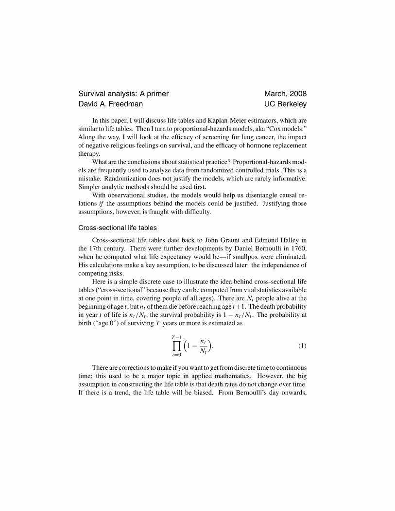
Survival analysis: A primer March, 2008David A. Freedman UC Berkeley

In this paper, I will discuss life tables and Kaplan-Meier estimators, which aresimilar to life tables. Then I turn to proportional-hazards models, aka “Cox models.”Along the way, I will look at the efficacy of screening for lung cancer, the impactof negative religious feelings on survival, and the efficacy of hormone replacementtherapy.

What are the conclusions about statistical practice? Proportional-hazards mod-els are frequently used to analyze data from randomized controlled trials. This is amistake. Randomization does not justify the models, which are rarely informative.Simpler analytic methods should be used first.

With observational studies, the models would help us disentangle causal re-lations if the assumptions behind the models could be justified. Justifying thoseassumptions, however, is fraught with difficulty.

Cross-sectional life tables

Cross-sectional life tables date back to John Graunt and Edmond Halley inthe 17th century. There were further developments by Daniel Bernoulli in 1760,when he computed what life expectancy would be—if smallpox were eliminated.His calculations make a key assumption, to be discussed later: the independence ofcompeting risks.

Here is a simple discrete case to illustrate the idea behind cross-sectional lifetables (“cross-sectional” because they can be computed from vital statistics availableat one point in time, covering people of all ages). There are Nt people alive at thebeginning of age t , butnt of them die before reaching age t+1. The death probabilityin year t of life is nt/Nt , the survival probability is 1 − nt/Nt . The probability atbirth (“age 0”) of surviving T years or more is estimated as

T−1∏t=0

(1 − nt

Nt

). (1)

There are corrections to make if you want to get from discrete time to continuoustime; this used to be a major topic in applied mathematics. However, the bigassumption in constructing the life table is that death rates do not change over time.If there is a trend, the life table will be biased. From Bernoulli’s day onwards,

2 David A. Freedman

death rates have been going down in the Western world; this was the beginningof the demographic transition (Kirk, 1996). Therefore, cross-sectional life tablesunderstate life expectancy.

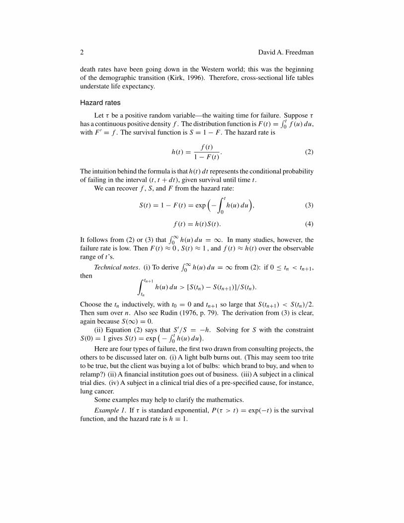
Hazard rates

Let τ be a positive random variable—the waiting time for failure. Suppose τhas a continuous positive density f . The distribution function isF(t) = ∫ t

0 f (u) du,with F ′ = f . The survival function is S = 1 − F . The hazard rate is

h(t) = f (t)

1 − F(t) . (2)

The intuition behind the formula is that h(t) dt represents the conditional probabilityof failing in the interval (t, t + dt), given survival until time t .

We can recover f , S, and F from the hazard rate:

S(t) = 1 − F(t) = exp(−

∫ t

0h(u) du

), (3)

f (t) = h(t)S(t). (4)

It follows from (2) or (3) that∫ ∞

0 h(u) du = ∞. In many studies, however, thefailure rate is low. Then F(t) ≈ 0 , S(t) ≈ 1 , and f (t) ≈ h(t) over the observablerange of t’s.

Technical notes. (i) To derive∫ ∞

0 h(u) du = ∞ from (2): if 0 ≤ tn < tn+1,then ∫ tn+1

tn

h(u) du > [S(tn)− S(tn+1)]/S(tn).

Choose the tn inductively, with t0 = 0 and tn+1 so large that S(tn+1) < S(tn)/2.Then sum over n. Also see Rudin (1976, p. 79). The derivation from (3) is clear,again because S(∞) = 0.

(ii) Equation (2) says that S′/S = −h. Solving for S with the constraintS(0) = 1 gives S(t) = exp

( − ∫ t0 h(u) du

).

Here are four types of failure, the first two drawn from consulting projects, theothers to be discussed later on. (i) A light bulb burns out. (This may seem too triteto be true, but the client was buying a lot of bulbs: which brand to buy, and when torelamp?) (ii) A financial institution goes out of business. (iii) A subject in a clinicaltrial dies. (iv) A subject in a clinical trial dies of a pre-specified cause, for instance,lung cancer.

Some examples may help to clarify the mathematics.

Example 1. If τ is standard exponential, P(τ > t) = exp(−t) is the survivalfunction, and the hazard rate is h ≡ 1.

Survival Analysis 3

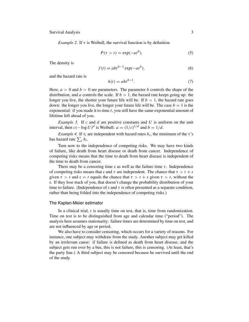
Example 2. If τ is Weibull, the survival function is by definition

P(τ > t) = exp(−atb). (5)

The density isf (t) = abtb−1 exp(−atb), (6)

and the hazard rate ish(t) = abtb−1. (7)

Here, a > 0 and b > 0 are parameters. The parameter b controls the shape of thedistribution, and a controls the scale. If b > 1, the hazard rate keeps going up: thelonger you live, the shorter your future life will be. If b < 1, the hazard rate goesdown: the longer you live, the longer your future life will be. The case b = 1 is theexponential: if you made it to time t , you still have the same exponential amount oflifetime left ahead of you.

Example 3. If c and d are positive constants and U is uniform on the unitinterval, then c(− logU)d is Weibull: a = (1/c)1/d and b = 1/d.

Example 4. If τi are independent with hazard rates hi , the minimum of the τ ’shas hazard rate

∑i hi .

Turn now to the independence of competing risks. We may have two kindsof failure, like death from heart disease or death from cancer. Independence ofcompeting risks means that the time to death from heart disease is independent ofthe time to death from cancer.

There may be a censoring time c as well as the failure time τ . Independenceof competing risks means that c and τ are independent. The chance that τ > t + sgiven τ > t and c = t equals the chance that τ > t + s given τ > t , without thec. If they lose track of you, that doesn’t change the probability distribution of yourtime to failure. (Independence of c and τ is often presented as a separate condition,rather than being folded into the independence of competing risks.)

The Kaplan-Meier estimator

In a clinical trial, t is usually time on test, that is, time from randomization.Time on test is to be distinguished from age and calendar time (“period”). Theanalysis here assumes stationarity: failure times are determined by time on test, andare not influenced by age or period.

We also have to consider censoring, which occurs for a variety of reasons. Forinstance, one subject may withdraw from the study. Another subject may get killedby an irrelevant cause: if failure is defined as death from heart disease, and thesubject gets run over by a bus, this is not failure, this is censoring. (At least, that’sthe party line.) A third subject may be censored because he survived until the endof the study.

4 David A. Freedman

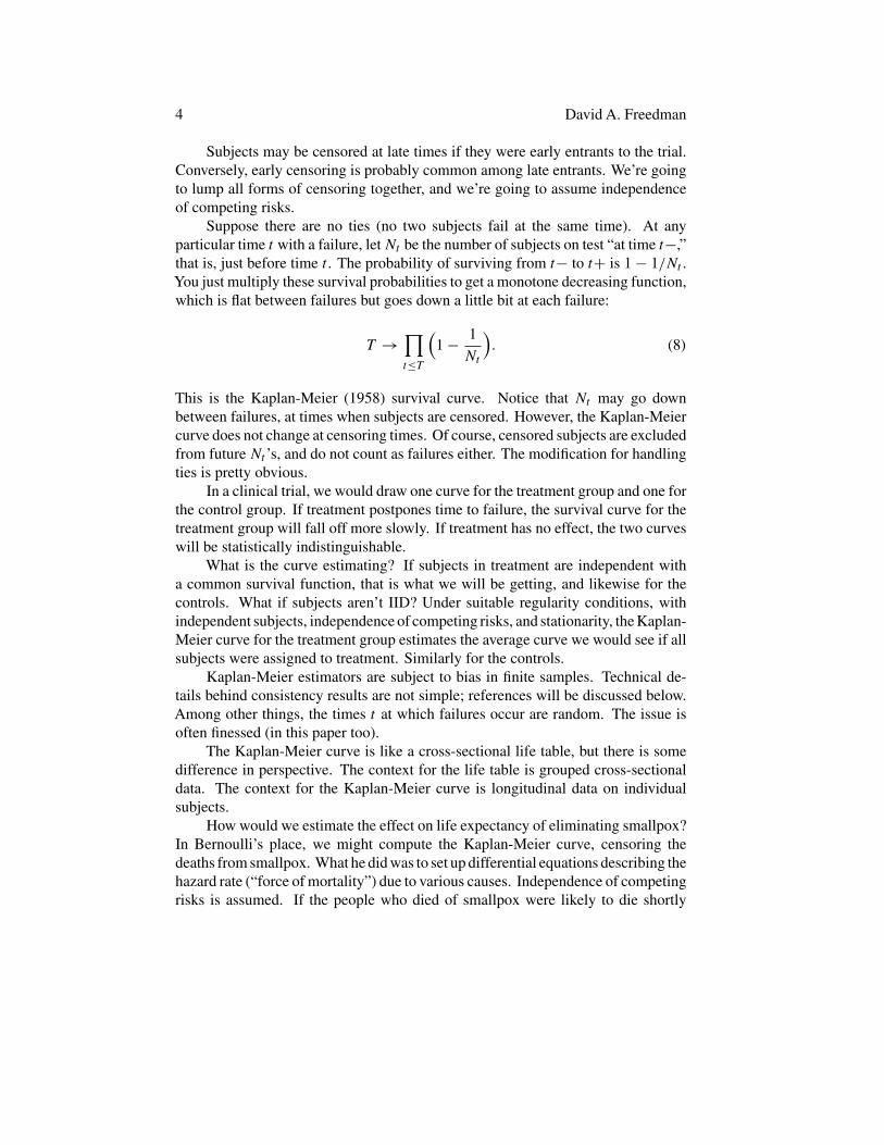
Subjects may be censored at late times if they were early entrants to the trial.Conversely, early censoring is probably common among late entrants. We’re goingto lump all forms of censoring together, and we’re going to assume independenceof competing risks.

Suppose there are no ties (no two subjects fail at the same time). At anyparticular time t with a failure, letNt be the number of subjects on test “at time t−,”that is, just before time t . The probability of surviving from t− to t+ is 1 − 1/Nt .You just multiply these survival probabilities to get a monotone decreasing function,which is flat between failures but goes down a little bit at each failure:

T →∏t≤T

(1 − 1

Nt

). (8)

This is the Kaplan-Meier (1958) survival curve. Notice that Nt may go downbetween failures, at times when subjects are censored. However, the Kaplan-Meiercurve does not change at censoring times. Of course, censored subjects are excludedfrom future Nt ’s, and do not count as failures either. The modification for handlingties is pretty obvious.

In a clinical trial, we would draw one curve for the treatment group and one forthe control group. If treatment postpones time to failure, the survival curve for thetreatment group will fall off more slowly. If treatment has no effect, the two curveswill be statistically indistinguishable.

What is the curve estimating? If subjects in treatment are independent witha common survival function, that is what we will be getting, and likewise for thecontrols. What if subjects aren’t IID? Under suitable regularity conditions, withindependent subjects, independence of competing risks, and stationarity, the Kaplan-Meier curve for the treatment group estimates the average curve we would see if allsubjects were assigned to treatment. Similarly for the controls.

Kaplan-Meier estimators are subject to bias in finite samples. Technical de-tails behind consistency results are not simple; references will be discussed below.Among other things, the times t at which failures occur are random. The issue isoften finessed (in this paper too).

The Kaplan-Meier curve is like a cross-sectional life table, but there is somedifference in perspective. The context for the life table is grouped cross-sectionaldata. The context for the Kaplan-Meier curve is longitudinal data on individualsubjects.

How would we estimate the effect on life expectancy of eliminating smallpox?In Bernoulli’s place, we might compute the Kaplan-Meier curve, censoring thedeaths from smallpox. What he did was to set up differential equations describing thehazard rate (“force of mortality”) due to various causes. Independence of competingrisks is assumed. If the people who died of smallpox were likely to die shortly

Survival Analysis 5

thereafter of something else anyway (“frailty”), we would all be over-estimating theimpact of eliminating smallpox.

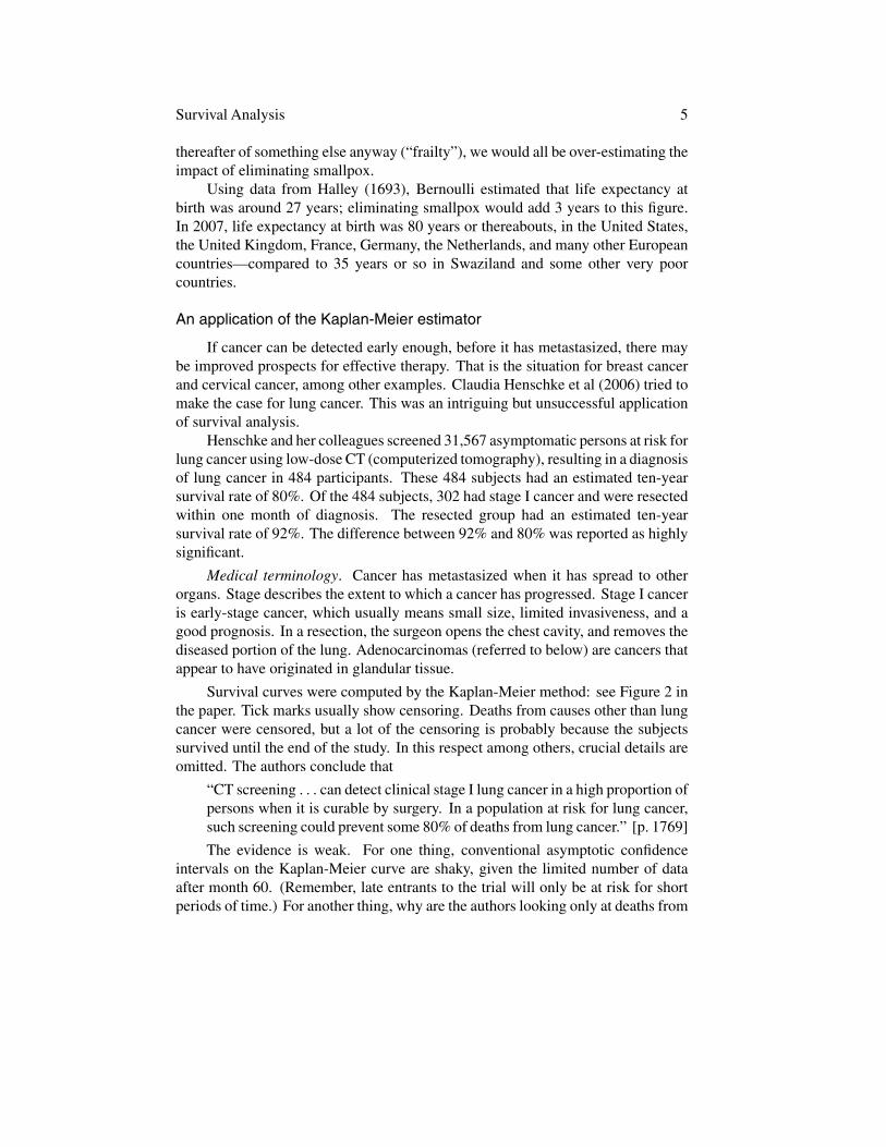
Using data from Halley (1693), Bernoulli estimated that life expectancy atbirth was around 27 years; eliminating smallpox would add 3 years to this figure.In 2007, life expectancy at birth was 80 years or thereabouts, in the United States,the United Kingdom, France, Germany, the Netherlands, and many other Europeancountries—compared to 35 years or so in Swaziland and some other very poorcountries.

An application of the Kaplan-Meier estimator

If cancer can be detected early enough, before it has metastasized, there maybe improved prospects for effective therapy. That is the situation for breast cancerand cervical cancer, among other examples. Claudia Henschke et al (2006) tried tomake the case for lung cancer. This was an intriguing but unsuccessful applicationof survival analysis.

Henschke and her colleagues screened 31,567 asymptomatic persons at risk forlung cancer using low-dose CT (computerized tomography), resulting in a diagnosisof lung cancer in 484 participants. These 484 subjects had an estimated ten-yearsurvival rate of 80%. Of the 484 subjects, 302 had stage I cancer and were resectedwithin one month of diagnosis. The resected group had an estimated ten-yearsurvival rate of 92%. The difference between 92% and 80% was reported as highlysignificant.

Medical terminology. Cancer has metastasized when it has spread to otherorgans. Stage describes the extent to which a cancer has progressed. Stage I canceris early-stage cancer, which usually means small size, limited invasiveness, and agood prognosis. In a resection, the surgeon opens the chest cavity, and removes thediseased portion of the lung. Adenocarcinomas (referred to below) are cancers thatappear to have originated in glandular tissue.

Survival curves were computed by the Kaplan-Meier method: see Figure 2 inthe paper. Tick marks usually show censoring. Deaths from causes other than lungcancer were censored, but a lot of the censoring is probably because the subjectssurvived until the end of the study. In this respect among others, crucial details areomitted. The authors conclude that

“CT screening . . . can detect clinical stage I lung cancer in a high proportion ofpersons when it is curable by surgery. In a population at risk for lung cancer,such screening could prevent some 80% of deaths from lung cancer.” [p. 1769]

The evidence is weak. For one thing, conventional asymptotic confidenceintervals on the Kaplan-Meier curve are shaky, given the limited number of dataafter month 60. (Remember, late entrants to the trial will only be at risk for shortperiods of time.) For another thing, why are the authors looking only at deaths from

6 David A. Freedman

lung cancer rather than total mortality? Next, stage I cancers—the kind detected bythe CT scan—are small. This augurs well for long-term survival, treatment or notreatment. Even more to the point, the cancers found by screening are likely to beslow-growing. That is “length bias.”

Table 3 in Henschke et al shows that most of the cancers were adenocarci-nomas; these generally have a favorable prognosis. Moreover, the cancer patientswho underwent resection were probably healthier to start with than the ones whodidn’t. In short, the comparison between the resection group and all lung cancers isuninformative. One of the things lacking in this study is a reasonable control group.

If screening speeds up detection, that will increase the time from detection todeath—even if treatment is ineffective. The increase is called “lead time” or “lead-time bias.” (To measure the effectiveness of screening, you might want to knowthe time from detection to death, net of lead time.) Lead time and length bias arediscussed in the context of breast cancer screening by Shapiro et al (1988).

When comparing their results to population data, Henschke et al measure ben-efits as the increase in time from diagnosis to death. This is misleading, as we havejust noted. CT scans speed up detection, but we do not know whether that helps thepatients live longer, because we do not know whether early treatment is effective.Henschke et al are assuming what needs to be proved. For additional discussion,see Patz et al (2000) and Welch et al (2007).

Lead time bias and length bias are problems for observational studies of screen-ing programs. Well-run clinical trials avoid such biases, if benefits are measured bycomparing death rates among those assigned to screening and those assigned to thecontrol group. This is an example of the intention-to-treat principle (Bradford Hill,1961, p. 259).

A hypothetical will clarify the idea of lead time. “Crypto-megalo-grandioma”(CMG) is a dreadful disease, which is rapidly fatal after diagnosis. Existing therapiesare excruciating and ineffective. No improvements are on the horizon. However,there is a screening technique that can reliably detect the disease 10 years before itbecomes clinically manifest. Will screening increase survival time from diagnosisto death? Do you want to be screened for CMG?

The proportional-hazards model in brief

Assume independence of competing risks; subjects are independent of oneanother; there is a baseline hazard rate h > 0, which is the same for all subjects.There is a vector of subject-specific characteristics Xit , which is allowed to varywith time. The subscript i indexes subjects and t indexes time. There is a parametervector β, which is assumed to be the same for all subjects and constant over time.Time can be defined in several ways. Here, it means time on test; but see Thiebautand Benichou (2004). The hazard rate for subject i is assumed to be

h(t) exp(Xitβ). (9)

Survival Analysis 7

No intercept is allowed: the intercept would get absorbed into h. The mostinteresting entry inXit is usually a dummy for treatment status. This is 1 for subjectsin the treatment group, and 0 for subjects in the control group. We pass over alltechnical regularity conditions in respectful silence.

The likelihood function is not a thing of beauty. To make this clear, we canwrite down the log likelihood function L(h, β), which is a function of the baselinehazard rate h and the parameter vector β. For the moment, we will assume there isno censoring and the Xit are constant (not random). Let τi be the failure time forsubject i. By (3)-(4),

L(h, β) =n∑i=1

log fi(τi |h, β), (10a)

where

fi(t |h, β) = hi(t |β) exp(−

∫ t

0hi(u|β) du

), (10b)

and

hi(t |β) = h(t) exp(Xitβ). (10c)

This is a mess, and maximizing over the infinite-dimensional parameter h is adaunting prospect.

Cox (1972) suggested proceeding another way. Suppose there is a failure attime t . Remember, t is time on test, not age or period. Consider the set Rt ofsubjects who were on test just before time t . These subjects have not failed yet, orbeen censored; so they are eligible to fail at time t . Suppose it was subject j whofailed. Heuristically, the chance of it being subject j rather than anybody else in therisk set is

h(t) exp(Xjtβ) dt∑i∈Rt h(t) exp(Xitβ) dt

= exp(Xjtβ)∑i∈Rt exp(Xitβ)

. (11)

Subject j is in numerator and denominator both, and by assumption there are noties: ties are a technical nuisance. The baseline hazard rate h(t) and the dt cancel!Now we can do business.

Multiply the right side of (11) over all failure times to get a “partial likelihoodfunction.” This is a function of β. Take logs and maximize to get β. Computethe Hessian—the second derivative matrix of the log partial likelihood—at β. Thenegative of the Hessian is the “observed partial information.” Invert this matrix toget the estimated variance-covariance matrix for the β’s. Take the square root of thediagonal elements to get asymptotic SEs.

Partial likelihood functions are not real likelihood functions. The harder youthink about (11) and the multiplication, the less sense it makes. The chance of whatevent, exactly? Conditional on what information? Failure times are random, not

8 David A. Freedman

deterministic; this is ignored by (11). The multiplication is bogus. For example,there is no independence: if Harriet is at risk at time T , she cannot have failed at anearlier time t . Still, there is mathematical theory to show that β performs like a realMLE, under the regularity conditions that we have passed over; also see Example 5below.

Proportional-hazards models are often used in observational studies and in clin-ical trials. The latter fact is a real curiosity. There is no need to adjust for confound-ing if the trial is randomized. Moreover, in a clinical trial, the proportional-hazardsmodel makes its calculations conditional on assignment. The random elements arethe failure times for the subjects. As far as the model is concerned, the randomizationis irrelevant. Equally, randomization does not justify the model.

A mathematical diversion

Example 5. Suppose the covariates Xit ≡ Xi do not depend on t and are non-stochastic; for instance, covariates are measured at recruitment into the trial and areconditioned out. Suppose there is no censoring. Then the partial likelihood functionis the ordinary likelihood function for the ranks of the failure times. Kalbfleisch andPrentice (1973) discuss more general results.

Sketch proof . The argument is not completely straightforward, and all theassumptions will be used. As a matter of notation, subject i has failure time τi . Thehazard rate of τi is h(t) exp(Xiβ), the density is fi(t), and the survival function isSi(t). Let ci = exp(Xiβ). We start with the case n = 2. Let C = c1 + c2. Use(3)-(4) to see that

P(τ1 < τ2) =∫ ∞

0S2(t)f1(t) dt

= c1

∫ ∞

0h(t)S1(t)S2(t) dt

= c1

∫ ∞

0h(t) exp

(− C

∫ t

0h(u)du

)dt. (12)

Last but not least,

C

∫ ∞

0h(t) exp

(− C

∫ t

0h(u)du

)dt = 1 (13)

by (4). So

P(τ1 < τ2) = c1

c1 + c2, (14)

as required.

Survival Analysis 9

Now suppose n > 2. The chance that τ1 is the smallest of the τ ’s is

c1

c1 + · · · + cn ,

as before: just replace τ2 by min {τ2, . . . , τn}. Given that τ1 = t and τ1 is the smallestof the τ ’s, the remaining τ ’s are independent and concentrated on (t,∞). If we lookat the random variables τi − t , their conditional distributions will have hazard ratescih(t + · ), so we can proceed inductively. A rigorous treatment might involveregular conditional distributions (Freedman, 1983, pp. 347ff). This completes thesketch proof.

Another argument, suggested by Russ Lyons, is to change the time scale so thehazard rate is identically 1. Under the conditions of Example 5, the transformationt → ∫ t

0 h(u) du reduces the general case to the exponential case. Indeed, if H isa continuous, strictly increasing function that maps [0,∞) onto itself, then H(τi)has survival function Si ◦H−1.

The mathematics does say something about statistical practice. At least inthe setting of Example 5, and contrary to general opinion, the model does not usetime-to-event data. It uses only the ranks: which subject failed first, which failedsecond, and so forth. That, indeed, is what enables the fitting procedure to getaround problems created by the intractable likelihood function.

An application of the proportional-hazards model

Pargament et al (2001) report on religious struggle as a predictor of mortalityamong very sick patients. Subjects were 596 mainly Baptist and Methodist patientsage 55+, hospitalized for serious illness at the Duke Medical Center and the DurhamVeterans’Affairs Medical Center. There was two-year followup, with 176 deaths and152 subjects lost to followup. Key variables of interest were positive and negativereligious feelings. There was adjustment by proportional hazards for age, race,gender, severity of illness, . . . , and for missing data.

The main finding reported by Pargament et al is that negative religious feelingsincrease the death rate. The authors say:

“Physicians are now being asked to take a spiritual history . . . . Our findingssuggest that patients who indicate religious struggle during a spiritual historymay be at particularly high risk . . . . Referral of these patients to clergy to helpthem work through these issues may ultimately improve clinical outcomes;further research is needed . . . .” [p. 1885]

The main evidence is a proportional-hazards model. Variables include age (in years),education (highest grade completed), race, gender, and . . . .

10 David A. Freedman

Religious feelings

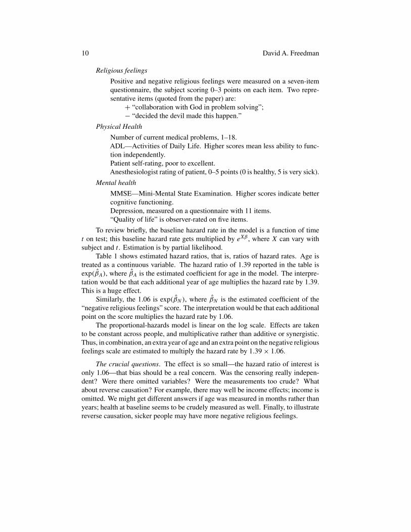
Positive and negative religious feelings were measured on a seven-itemquestionnaire, the subject scoring 0–3 points on each item. Two repre-sentative items (quoted from the paper) are:

+ “collaboration with God in problem solving”;− “decided the devil made this happen.”

Physical Health

Number of current medical problems, 1–18.ADL—Activities of Daily Life. Higher scores mean less ability to func-tion independently.Patient self-rating, poor to excellent.Anesthesiologist rating of patient, 0–5 points (0 is healthy, 5 is very sick).

Mental health

MMSE—Mini-Mental State Examination. Higher scores indicate bettercognitive functioning.Depression, measured on a questionnaire with 11 items.“Quality of life” is observer-rated on five items.

To review briefly, the baseline hazard rate in the model is a function of timet on test; this baseline hazard rate gets multiplied by eXβ , where X can vary withsubject and t . Estimation is by partial likelihood.

Table 1 shows estimated hazard ratios, that is, ratios of hazard rates. Age istreated as a continuous variable. The hazard ratio of 1.39 reported in the table isexp(βA), where βA is the estimated coefficient for age in the model. The interpre-tation would be that each additional year of age multiplies the hazard rate by 1.39.This is a huge effect.

Similarly, the 1.06 is exp(βN ), where βN is the estimated coefficient of the“negative religious feelings” score. The interpretation would be that each additionalpoint on the score multiplies the hazard rate by 1.06.

The proportional-hazards model is linear on the log scale. Effects are takento be constant across people, and multiplicative rather than additive or synergistic.Thus, in combination, an extra year of age and an extra point on the negative religiousfeelings scale are estimated to multiply the hazard rate by 1.39 × 1.06.

The crucial questions. The effect is so small—the hazard ratio of interest isonly 1.06—that bias should be a real concern. Was the censoring really indepen-dent? Were there omitted variables? Were the measurements too crude? Whatabout reverse causation? For example, there may well be income effects; income isomitted. We might get different answers if age was measured in months rather thanyears; health at baseline seems to be crudely measured as well. Finally, to illustratereverse causation, sicker people may have more negative religious feelings.

Survival Analysis 11

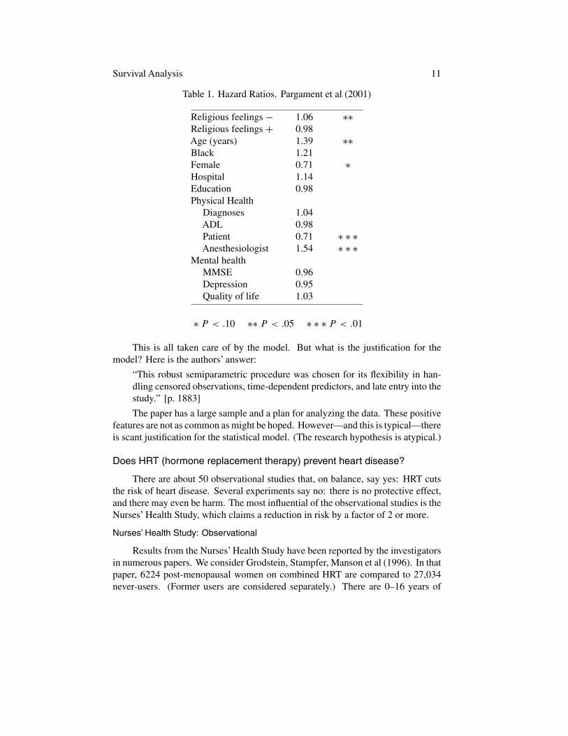
Table 1. Hazard Ratios. Pargament et al (2001)

Religious feelings − 1.06 ∗∗Religious feelings + 0.98Age (years) 1.39 ∗∗Black 1.21Female 0.71 ∗Hospital 1.14Education 0.98Physical Health

Diagnoses 1.04ADL 0.98Patient 0.71 ∗ ∗ ∗Anesthesiologist 1.54 ∗ ∗ ∗

Mental healthMMSE 0.96Depression 0.95Quality of life 1.03

∗ P < .10 ∗∗ P < .05 ∗ ∗ ∗ P < .01

This is all taken care of by the model. But what is the justification for themodel? Here is the authors’ answer:

“This robust semiparametric procedure was chosen for its flexibility in han-dling censored observations, time-dependent predictors, and late entry into thestudy.” [p. 1883]

The paper has a large sample and a plan for analyzing the data. These positivefeatures are not as common as might be hoped. However—and this is typical—thereis scant justification for the statistical model. (The research hypothesis is atypical.)

Does HRT (hormone replacement therapy) prevent heart disease?

There are about 50 observational studies that, on balance, say yes: HRT cutsthe risk of heart disease. Several experiments say no: there is no protective effect,and there may even be harm. The most influential of the observational studies is theNurses’ Health Study, which claims a reduction in risk by a factor of 2 or more.

Nurses’ Health Study: Observational

Results from the Nurses’ Health Study have been reported by the investigatorsin numerous papers. We consider Grodstein, Stampfer, Manson et al (1996). In thatpaper, 6224 post-menopausal women on combined HRT are compared to 27,034never-users. (Former users are considered separately.) There are 0–16 years of


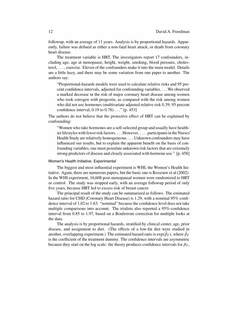
followup, with an average of 11 years. Analysis is by proportional hazards. Appar-ently, failure was defined as either a non-fatal heart attack, or death from coronaryheart disease.

The treatment variable is HRT. The investigators report 17 confounders, in-cluding age, age at menopause, height, weight, smoking, blood pressure, choles-terol, . . . , exercise. Eleven of the confounders make it into the main model. Detailsare a little hazy, and there may be some variation from one paper to another. Theauthors say:

“Proportional-hazards models were used to calculate relative risks and 95 per-cent confidence intervals, adjusted for confounding variables. . . .We observeda marked decrease in the risk of major coronary heart disease among womenwho took estrogen with progestin, as compared with the risk among womenwho did not use hormones (multivariate adjusted relative risk 0.39; 95 percentconfidence interval, 0.19 to 0.78). . . .” [p. 453]

The authors do not believe that the protective effect of HRT can be explained byconfounding:

“Women who take hormones are a self-selected group and usually have health-ier lifestyles with fewer risk factors. . . .However, . . . .participants in the Nurses’Health Study are relatively homogeneous. . . .Unknown confounders may haveinfluenced our results, but to explain the apparent benefit on the basis of con-founding variables, one must postulate unknown risk factors that are extremelystrong predictors of disease and closely associated with hormone use.” [p. 458]

Women’s Health Initiative: Experimental

The biggest and most influential experiment is WHI, the Women’s Health Ini-tiative. Again, there are numerous papers, but the basic one is Rossouw et al (2002).In the WHI experiment, 16,608 post-menopausal women were randomized to HRTor control. The study was stopped early, with an average followup period of onlyfive years, because HRT led to excess risk of breast cancer.

The principal result of the study can be summarized as follows. The estimatedhazard ratio for CHD (Coronary Heart Disease) is 1.29, with a nominal 95% confi-dence interval of 1.02 to 1.63: “nominal” because the confidence level does not takemultiple comparisons into account. The trialists also reported a 95%-confidenceinterval from 0.85 to 1.97, based on a Bonferroni correction for multiple looks atthe data.

The analysis is by proportional hazards, stratified by clinical center, age, priordisease, and assignment to diet. (The effects of a low-fat diet were studied inanother, overlapping experiment.) The estimated hazard ratio is exp(βT ), where βTis the coefficient of the treatment dummy. The confidence intervals are asymmetricbecause they start on the log scale: the theory produces confidence intervals for βT ,


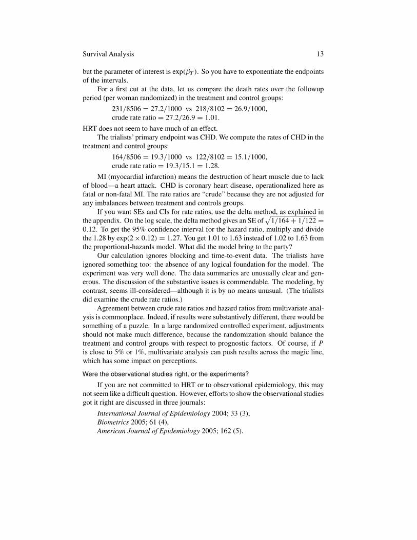
but the parameter of interest is exp(βT ). So you have to exponentiate the endpointsof the intervals.

For a first cut at the data, let us compare the death rates over the followupperiod (per woman randomized) in the treatment and control groups:

231/8506 = 27.2/1000 vs 218/8102 = 26.9/1000,crude rate ratio = 27.2/26.9 = 1.01.

HRT does not seem to have much of an effect.The trialists’ primary endpoint was CHD. We compute the rates of CHD in the

treatment and control groups:

164/8506 = 19.3/1000 vs 122/8102 = 15.1/1000,crude rate ratio = 19.3/15.1 = 1.28.

MI (myocardial infarction) means the destruction of heart muscle due to lackof blood—a heart attack. CHD is coronary heart disease, operationalized here asfatal or non-fatal MI. The rate ratios are “crude” because they are not adjusted forany imbalances between treatment and controls groups.

If you want SEs and CIs for rate ratios, use the delta method, as explained inthe appendix. On the log scale, the delta method gives an SE of

√1/164 + 1/122 =

0.12. To get the 95% confidence interval for the hazard ratio, multiply and dividethe 1.28 by exp(2 × 0.12) = 1.27. You get 1.01 to 1.63 instead of 1.02 to 1.63 fromthe proportional-hazards model. What did the model bring to the party?

Our calculation ignores blocking and time-to-event data. The trialists haveignored something too: the absence of any logical foundation for the model. Theexperiment was very well done. The data summaries are unusually clear and gen-erous. The discussion of the substantive issues is commendable. The modeling, bycontrast, seems ill-considered—although it is by no means unusual. (The trialistsdid examine the crude rate ratios.)

Agreement between crude rate ratios and hazard ratios from multivariate anal-ysis is commonplace. Indeed, if results were substantively different, there would besomething of a puzzle. In a large randomized controlled experiment, adjustmentsshould not make much difference, because the randomization should balance thetreatment and control groups with respect to prognostic factors. Of course, if Pis close to 5% or 1%, multivariate analysis can push results across the magic line,which has some impact on perceptions.

Were the observational studies right, or the experiments?

If you are not committed to HRT or to observational epidemiology, this maynot seem like a difficult question. However, efforts to show the observational studiesgot it right are discussed in three journals:

International Journal of Epidemiology 2004; 33 (3),Biometrics 2005; 61 (4),American Journal of Epidemiology 2005; 162 (5).


For the Nurses’ study, the argument is that HRT should start right after meno-pause, whereas in the WHI experiment, many women in treatment started HRT later.The WHI investigators ran an observational study in parallel with the experiment.This observational study showed the usual benefits. The argument here is that HRTcreates an initial period of risk, after which the benefits start. Neither of thesetiming hypotheses is fully consistent with the data, nor are the two hypothesesentirely consistent with each other (Petitti and Freedman, 2005). Results from latefollowup of WHI show an increased risk of cancer in the HRT group, which furthercomplicates the timing hypothesis (Heiss et al, 2008).

For reviews skeptical of HRT, see Petitti (1998, 2002). If the observationalstudies got it wrong, confounding is the likely explanation. An interesting possibilityis “prevention bias” or “complier bias” (Barrett-Connor, 1991; Petitti, 1994). Inbrief, subjects who follow doctors’ orders tend to do better, even when the ordersare to take a placebo. In the Nurses’ study, taking HRT seems to be thoroughlyconfounded with compliance.

In the clofibrate trial (Freedman-Pisani-Purves, 2007, pp. 14, A-4), compliershad half the death rate of non-compliers—in the drug group and the placebo groupboth. Interestingly, the difference between compliers and non-compliers could notbe predicted using baseline risk factors.

Another example is the HIP trial (Freedman, 2005, pp. 4–5). If you comparewomen who accepted screening for breast cancer to women who refused, the firstgroup had a 30% lower risk of death from causes other than breast cancer. Here,the compliance effect can be explained, to some degree, in terms of education andincome. Of course, the Nurses’ Health Study rarely adjusts for such variables.

Many other examples are discussed in Petitti and Chen (2008). For instance,using sunblock reduces the risk of heart attacks by a factor of 2; this estimate isrobust when adjustments are made for covariates.

Women who take HRT are women who see a doctor regularly. These womenare at substantially lower risk of death from a wide variety of diseases (Grodstein etal, 1997). The list includes diseases where HRT is not considered to be protective.The list also includes diseases like breast cancer, where HRT is known to be harmful.Grodstein et al might object that, in their multivariate proportional-hazards model,the hazard ratio for breast cancer isn’t quite significant—either for current users orformer users, taken separately.

Simulations

If the proportional-hazards model is right or close to right, it works pretty well.Precise measures of the covariates are not essential. If the model is wrong, there issomething of a puzzle: what is being estimated by fitting the model to the data? Onepossible answer is the crude rate ratio in a very large study population. We beginwith an example where the model works, then consider an example in the oppositedirection.


The model works

Suppose the baseline distribution of time to failure for untreated subjects isstandard exponential. There is a subject-specific random variable Wi which multi-plies the baseline time and gives the time to failure for subject i if untreated. Thehazard rate for subject i is therefore 1/Wi times the baseline hazard rate. By con-struction, the Wi are independent and uniform on [0, 1]. Treatment doubles thefailure time, that is, cuts the hazard rate in half—for every subject. We censor attime 0.10, which keeps the failure rates moderately realistic.

We enter logWi as the covariate. This is exactly the right covariate. The setupshould be duck soup for the model. We can look at simulation data on 5000 subjects,randomized to treatment or control by the toss of a coin. The experiment is repeated100 times.

The crude rate ratio is 0.620 ± 0.037. (In other words, the average across therepetitions is 0.620, and the SD is 0.037.)

The model with no covariate estimates the hazard ratio as 0.581 ± 0.039.

The model with the covariate logWi estimates the hazard ratio as 0.498±0.032.

The estimated hazard ratio is exp(βT ), where βT is the coefficient of the treat-ment dummy in the fitted model. The “real” ratio is 0.50. If that’s what you want,the full model looks pretty good. The no-covariate model goes wrong because itfails to adjust for logWi . This is complicated: logWi is nearly balanced between thetreatment and control groups, so it is not a confounder. However, without logWi ,the model is no good: subjects do not have a common baseline hazard rate. TheCox model is not “collapsible.”

The crude rate ratio (the failure rate in the treatment arm divided by the failurerate in the control arm) is very close to the true value, which is

1 − E[exp(0.05/Wi)]

1 − E[exp(0.10/Wi)]. (15)

The failure rates in treatment and control are about 17% and 28%, big enough sothat the crude rate ratio is somewhat different from the hazard ratio: 1/Wi has along, long tail. In this example and many others, the crude rate ratio seems to be auseful summary statistic.

The model is somewhat robust against measurement error. For instance, sup-pose there is a biased measurement of the covariate: we enter

√ − logWi into themodel, rather than logWi . The estimated hazard ratio is 0.516 ± 0.030, so the biasin the hazard ratio—created by the biased measurement of the covariate—is only0.016. Of course, if we degrade the measurement further, the model will performworse. If the covariate is

√ − logWi + logUi where Ui is an independent uniformvariable, the estimate is noticeably biased: 0.574 ± 0.032.


The model does not work

We modify the previous construction a little. To begin with, we dropWi . Thetime to failure if untreated (τi) is still standard exponential, and we still censor attime 0.10. As before, the effect of treatment is to double τi , which cuts the hazardrate in half. So far, so good: we are still on home ground for the model.

The problem is that we have a new covariate,

Zi = exp(−τi)+ cUi, (16)

where Ui is an independent uniform variable and c is a constant. Notice thatexp(−τi) is itself uniform. The hapless statistician in this fable will have the dataon Zi , but will not know how the data were generated.

The simple proportional-hazards model, without covariates, matches the cruderate ratio. If we enter the covariate into the model, all depends on c. Here are theresults for c = 0.

The crude rate ratio is 0.510 ± 0.063. (The true value is 1.10/2.10 ≈ 0.524.)


The model with the covariate (16) estimates the hazard ratio as 0.001 ± 0.001.

The crude rate ratio looks good, and so does the no-covariate model. However,the model with the covariate says that treatment divides the hazard rate by 1000.Apparently, this is the wrong kind of covariate to put into the model.

If c = 1, so that noise offsets the signal in the covariate, the full model estimatesa hazard ratio of about 0.45—somewhat too low. If c = 2, noise swamps the (bad)signal, and the full model works fine. There is actually a little bit of variancereduction.

Some observers may object that (16) is not a confounder, because (on average)there will be balance between treatment and control. To meet that objection, justchange the covariate to

Zi = exp(−τi)+ ζi exp(−τi/2)+ cUi, (17)

where ζi is the treatment dummy. The covariate (17) is unbalanced between treat-ment and control groups. It is related to outcomes. It contains valuable information.In short, it is a classic example of a confounder. But, for the proportional-hazardsmodel, it’s the wrong kind of confounder—poison, unless c is quite large.

Here are the results for c = 2, when half the variance in (17) is accounted forby noise, so there is a lot of dilution.

The crude rate ratio is 0.522 ± 0.056.


The model with the covariate (17) estimates the hazard ratio as 0.165 ± 0.138.


(We have independent randomization across examples, which is how 0.510 in theprevious example changed to 0.522 here.) Putting the covariate (17) into the modelbiases the hazard ratio downwards by a factor of 3.

What is wrong with these covariates? The proportional-hazards model is notonly about adjusting for confounders, it is also about hazards that are proportional tothe baseline hazard. The key assumption in the model is something like this. Giventhat a subject is alive and uncensored at time t , and given the covariate history up totime t , the probability of failure in (t, t + dt) is h(t) exp(Xitβ) dt , where h is thebaseline hazard rate. In (16) with c = 0, the conditional failure time will be known,because Zi determines τi . So the key assumption in the model breaks down. If c issmall, the situation is similar, as it is for the covariate in (17).

Some readers may ask whether problems can be averted by judicious use ofmodel diagnostics. No doubt, if we start with a well-defined type of breakdownin modeling assumptions, there are diagnostics that will detect the problem. Con-versely, if we fix a suite of diagnostics, there are problems that will evade detection(Freedman, 2008a).

Causal inference from observational data

Freedman (2005) reviews a logical framework, based on Neyman (1923), inwhich regression can be used to infer causation. There is a straightforward extensionto the Cox model with non-stochastic covariates. Beyond the purely statisticalassumptions, the chief additional requirement is “invariance to intervention.” Inbrief, manipulating treatment status should not change the statistical relations.

For example, suppose a subject chose the control condition, but we want toknow what would have happened if we had put him into treatment. Mechanically,nothing is easier: just switch the treatment dummy from 0 to 1, and compute thehazard rate accordingly. Conceptually, however, we are assuming that the inter-vention would not have changed the baseline hazard rate, or the values of the othercovariates, or the coefficients in the model.

Invariance is a heroic assumption. How could you begin to verify it, without ac-tually doing the experiment and intervening? That is one of the essential difficultiesin using models to make causal inferences from non-experimental data.

What is the bottom line?

There needs to be some hard thinking about the choice of covariates, theproportional-hazards assumption, the independence of competing risks, and so forth.In the applied literature, these issues are rarely considered in any depth. That is whythe modeling efforts, in observational studies as in experiments, are often uncon-vincing.

Cox (1972) grappled with the question of what the proportional hazards modelwas good for. He ends up by saying


“[i] Of course, the [model] outlined here can be made much more specific byintroducing explicit stochastic processes or physical models. The wide varietyof possibilities serves to emphasize the difficulty of inferring an underlyingmechanism indirectly from failure times alone rather than from direct studyof the controlling physical processes. [ii] As a basis for rather empirical datareduction, [the model] seems flexible and satisfactory.” [p. 201]

The first point is undoubtedly correct, although it is largely ignored by practitioners.The second point is at best debatable. If the model is wrong, why are the parameterestimates a good summary of the data? In any event, questions about summarystatistics seem largely irrelevant: practitioners fit the model to the data withoutconsidering assumptions, and leap to causal conclusions.

Where do we go from here?

I will focus on clinical trials. Altman, Schulz, and Moher et al (2001) doc-ument persistent failures in the reporting of the data, and make detailed proposalsfor improvement. The following recommendations are complementary; also seeAndersen (1991).

(i) As is usual, measures of balance between the assigned-to-treatment groupand the assigned-to-control group should be reported.

(ii) After that should come a simple intention-to-treat analysis, comparing rates(or averages and SDs) among those assigned to treatment and those assigned to thecontrol group.

(iii) Crossover should be discussed, and deviations from protocol.

(iv) Subgroup analyses should be reported, and corrections for crossover ifthat is to be attempted. Two sorts of corrections are increasingly common. (a) Per-protocol analysis censors subjects who cross over from one arm of the trial tothe other, for instance, subjects who are assigned to control but insist on treatment.(b) Analysis by treatment received compares those who receive treatment with thosewho do not, regardless of assignment. These analyses require special justification(Freedman, 2006).

(v) Regression estimates (including logistic regression and proportional haz-ards) should be deferred until rates and averages have been presented. If regressionestimates differ from simple intention-to-treat results, and reliance is placed on themodels, that needs to be explained. The usual models are not justified by random-ization, and simpler estimators may be more robust.

(vi) The main assumptions in the models should be discussed. Which oneshave been checked. How? Which of the remaining assumptions are thought to bereasonable? Why?

(vii) Authors should distinguish between analyses specified in the trial protocoland other analyses. There is much to be said for looking at the data; but readers need


to know how much looking was involved, before that significant difference poppedout.

(viii) The exact specification of the models used should be posted on journalwebsites, including definitions of the variables. The underlying data should beposted too, with adequate documentation. Patient confidentiality would need to beprotected, and authors may deserve a grace period after first publication to furtherexplore the data.

Some studies make data available to selected investigators under stringent con-ditions (Geller et al., 2004), but my recommendation is different. When data-collection efforts are financed by the public, the data should be available for publicscrutiny.

Some pointers to the literature

Early publications on vital statistics and life tables include Graunt (1662),Halley (1693), and Bernoulli (1760). Bernoulli’s calculations on smallpox mayseem a bit mysterious. For discussion, including historical context, see Gani (1978)or Dietz and Hesterbeek (2002). A useful book on the early history of statistics,including life tables, is Hald (2005).

Freedman (2007, 2008b) discusses the use of models to analyze experimentaldata. In brief, the advice is to do it late if at all. Fremantle et al. (2003) have a criticaldiscussion on use of “composite endpoints,” which combine data on many distinctendpoints. An example, not much exaggerated, would be fatal MI + non-fatal MI +angina + heartburn.

Typical presentations of the proportional-hazards model (this one included) in-volve a lot of hand-waving. It is possible to make math out the hand-waving. But thisgets very technical very fast, with martingales, compensators, left-continuous filtra-tions, and the like. One of the first rigorous treatments was OddAalen’s Ph. D. thesisat Berkeley, written under the supervision of Lucien LeCam. See Aalen (1978) forthe published version, which builds on related work by Pierre Bremaud and JeanJacod.

Survival analysis is sometimes viewed as a special case of “event history anal-ysis.” Standard mathematical references include Andersen et al (1996), Flemingand Harrington (2005). A popular alternative is Kalbfleisch and Prentice (2002).Some readers like Miller (1998); others prefer Lee and Wang (2003). Jewell (2003)is widely used. Technical details in some of these texts may not be in perfect focus.If you want mathematical clarity, Aalen (1978) is still a paper to be recommended.

For a detailed introduction to the subject, look at Andersen and Keiding (2006).This book is organized as a one-volume encyclopedia. Peter Sasieni’s entry on the“Cox Regression Model” is a good starting point; after that, just browse. Lawless(2003) is another helpful reference.


Appendix: The delta method in more detail

The context for this discussion is the Women’s Health Initiative, a randomizedcontrolled experiment on the effects of hormone replacement therapy. Let N andN ′ be the numbers of women randomized to treatment and control. Let ξ and ξ ′ bethe corresponding numbers of failures (that is, for instance, fatal or non-fatal heartattacks).

The crude rate ratio is the failure rate in the treatment arm divided by therate in the control arm, with no adjustments whatsoever. Algebraically, this is(ξ/N)

/(ξ ′/N ′). The logarithm of the crude rate ratio is

log ξ − log ξ ′ − logN + logN ′. (18)

Let µ = E(ξ). So

log ξ = log[µ

(1 + ξ − µ

µ

)]

= logµ+ log(

1 + ξ − µµ

)

≈ logµ+ ξ − µµ

, (19)

because log(1 + h) ≈ h when h is small. The delta-method ≈ a one-term Taylorseries.

For present purposes, take ξ to be approximately Poisson, so var(ξ) ≈ µ ≈ ξ

and

var(ξ − µµ

)≈ 1

µ≈ 1

ξ. (20)

A similar calculation can be made for ξ ′. Take ξ and ξ ′ to be approximately in-dependent, so the log of the crude rate ratio has variance approximately equal to1/ξ + 1/ξ ′.

The modeling is based on the idea that each subject has a small probability offailing during the trial. This probability is modifiable by treatment. Probabilities andeffects of treatment may differ from one subject to another. Subjects are assumedto be independent, and calculations are conditional on assignment.

Exact combinatorial calculations can be made, unconditionally, based on thepermutations used in the randomization. To take blocking, censoring, or time-to-failure into account, unpublished data would usually be needed.

For additional information on the delta method, see van derVaart (1998). Manyarguments for asymptotic behavior of the MLE turn out to depend on more rigorous(or less rigorous) versions of the delta method. Similar comments apply to theKaplan-Meier estimator.


References

Aalen, O. O. (1978). “Nonparametric Inference for a Family of Counting Processes,”Annals of Statistics, 6, 701–26.

Altman, D. G., Schulz, K. F., David Moher et al. (2001). “The Revised CONSORTStatement for Reporting Randomized Trials: Explanation and Elaboration,” Annalsof Internal Medicine, 134, 663–94.

Andersen, P. K. (1991). “Survival Analysis 1982–1991: The Second Decade of theProportional Hazards Regression Model,” Statistics in Medicine, 10, 1931–41.

Andersen, P. K., Borgan, Ø., Gill, R. D., and Keiding, N. (1996). Statistical ModelsBased on Counting Processes. Corr. 4th printing. New York: Springer-Verlag.

Andersen, P. K. and Keiding, N. eds. (2006). Survival and Event History Analysis.Chichester, U. K.: John Wiley & Sons.

Barrett-Connor, E. (1991). “Postmenopausal Estrogen and Prevention Bias,” Annalsof Internal Medicine, 115, 455–56.

Bernoulli, D. (1760). “Essai d’une nouvelle analyse de la mortalite causee par lapetite variole, et des avantages de l’inoculation pour la prevenir,” Memoires deMathematique et de Physique de l’Academie Royale des Sciences, Paris, 1–45.Reprinted in Histoire de l’Academie Royale des Sciences (1766) .

Cox, D. (1972). “Regression Models and Lifetables,” Journal of the Royal StatisticalSociety, Series B, 34, 187–220 (with discussion).

Dietz, K. and Heesterbeek, J. A. P. (2002). “Daniel Bernoulli’s EpidemiologicalModel Revisited,” Mathematical Biosciences, 180, 1–21.

Fleming, T. R. and Harrington, D. P. (2005). Counting Processes and Survival Anal-ysis. 2nd rev. edn. New York: John Wiley & Sons.

Freedman, D. A. (1983). Markov Chains. New York: Springer-Verlag.

Freedman, D. A. (2005). Statistical Models: Theory and Practice. New York: Cam-bridge University Press.

Freedman, D. A. (2006). “Statistical Models for Causation: What Inferential Lever-age Do They Provide?” Evaluation Review, 30, 691–713.

http://www.stat.berkeley.edu/users/census/oxcauser.pdf

Freedman, D. A. (2007). “On Regression Adjustments in Experiments with SeveralTreatments,” To appear in Annals of Applied Statistics.

http://www.stat.berkeley.edu/users/census/neyregcm.pdf

Freedman, D. A. (2008a). “Diagnostics Cannot Have Much Power Against GeneralAlternatives.”

http://www.stat.berkeley.edu/users/census/notest.pdf

Freedman, D. A. (2008b). “Randomization Does Not Justify Logistic Regression.”http://www.stat.berkeley.edu/users/census/neylogit.pdf


Freedman, D. A., Purves, R. A., and Pisani R. (2007). Statistics. 4th edn. New York:W. W. Norton & Co., Inc.

Fremantle, N., Calvert, M., Wood, J. et al. (2003). “Composite Outcomes in Ran-domized Trials: Greater Precision But With Greater Uncertainty?” Journal of theAmerican Medical Association, 289, 2554–59.

Gani, J. (1978). “Some Problems of Epidemic Theory,” Journal of the Royal Statis-tical Society, Series A, 141, 323–47 (with discussion).

Geller, N. L., Sorlie, P., Coady, S., Fleg, J., and Friedman, L. (2004). Limited accessdata sets from studies funded by the National Heart, Lung, and Blood Institute.Clinical Trials, 1, 517–524.

Graunt, J. (1662). Natural and Political Observations Mentioned in a followingIndex, and Made upon the Bills of Mortality. London. Printed by Tho. Roycroft,forJohn Martin, James Allestry, and Tho. Dicas, at the Sign of the Bell in St. Paul’sChurch-yard, MDCLXII. Available on-line at

http://www.ac.wwu.edu/˜stephan/Graunt/There is a life table on page 62. Reprinted by Ayer Company Publishers, NH, 2006.

Grodstein, F., Stampfer, M. J., Manson, J. et al. (1996). “Postmenopausal Estrogenand Progestin Use and the Risk of Cardiovascular Disease,” New England Journalof Medicine, 335, 453–61.

Grodstein, F., Stampfer, M. J., Colditz, G. A. et al. (1997). “Postmenopausal Hor-mone Therapy and Mortality,” New England Journal of Medicine, 336, 1769–75.

Hald, A. (2005). A History of Probability and Statistics and Their Applicationsbefore 1750. New York: John Wiley & Sons.

Halley, E. (1693). “An Estimate of the Mortality of Mankind, Drawn from CuriousTables of the Births and Funerals at the City of Breslaw; with anAttempt toAscertainthe Price of Annuities upon Lives,” Philosophical Transactions of the Royal Societyof London, 196, 596–610, 654–56.

Heiss, G., Wallace, R., Anderson, G. L., et al. (2008). “Health Risks and Benefits 3Years After Stopping Randomized Treatment With Estrogen and Progestin,” Journalof the American Medical Association, 299, 1036–45.

Henschke, C. I., Yankelevitz, D. F., Libby, D. M. et al. (2006). “The InternationalEarly Lung Cancer Action Program Investigators. Survival of Patients with Stage ILung Cancer Detected on CT Screening,” New England Journal of Medicine, 355,1763–71.

Hill, A. B. (1961). Principles of Medical Statistics. 7th ed. London: The Lancet.

Jewell, N. P. (2003). Statistics for Epidemiology. Boca Raton, FL: Chapman &Hall/CRC.

Kalbfleisch, J. D. and Prentice, R. L. (1973). “Marginal Likelihoods Based on Cox’sRegression and Life Model,” Biometrika, 60, 267–78.


Kalbfleisch, J. D. and Prentice, R. L. (2002). The Statistical Analysis of Failure TimeData. 2nd ed. New York: John Wiley & Sons.

Kaplan, E. L. and Meier, P. (1958). “Nonparametric Estimation from IncompleteObservations,” Journal of American Statistical Association, 53, 457–81.

Kirk, D. (1996). “Demographic Transition Theory,” Population Studies, 50, 361–87.

Lawless, J. F. (2003). Statistical Models and Methods for Lifetime Data. 2nd ed.New York: John Wiley & Sons.

Lee, E. T. and Wang, J. W. (2003). Statistical Methods for Survival Data Analysis.3rd ed. New York: John Wiley & Sons.

Miller, R. G., Jr. (1998). Survival Analysis. New York: John Wiley & Sons.

Neyman, J. (1923). Sur les applications de la theorie des probabilites aux experiencesagricoles: Essai des principes. Roczniki Nauk Rolniczych 10: 1–51, in Polish. Englishtranslation by Dabrowska, D. M. and Speed, T. P. (1990), Statistical Science, 5, 465–80 (with discussion).

Pargament, K. I., Koenig, H. G., Tarakeshwar, N., and Hahn, J. (2001). “ReligiousStruggle as a Predictor of Mortality among Medically Ill Patients,” Archives ofInternal Medicine, 161, 1881–85.

Patz, E. F., Jr., Goodman, P. C., and Bepler, G. (2000). “Screening for Lung Cancer,”New England Journal of Medicine, 343, 1627–33.

Petitti, D. B. (1994). “Coronary Heart Disease and Estrogen Replacement Therapy:Can Compliance Bias Explain the Results of Observational Studies?” Annals ofEpidemiology, 4, 115–18.

Petitti, D. B. (1998). “Hormone Replacement Therapy and Heart Disease Prevention:Experimentation Trumps Observation,” Journal of the American Medical Associa-tion, 280, 650–51.

Petitti, D. B. (2002). “Hormone Replacement Therapy for Prevention,” Journal ofthe American Medical Association, 288, 99–101.

Petitti, D. B. and Freedman, D. A. (2005). “Invited Commentary: How Far Can Epi-demiologists Get with Statistical Adjustment?” American Journal of Epidemiology,162, 415–18.

Petitti, D. B. and Chen, W. (2008). “Statistical Adjustment for a Measure of HealthyLifestyle Doesn’tYield the Truth about Hormone Therapy,” to appear in Probabilityand Statistics: Essays in Honor of David A. Freedman, eds. Deborah Nolan andTerry Speed. Institute of Mathematical Statistics.

Rossouw, J. E., Anderson, G. L., Prentice, R. L. et al. (2002). “Risks and Benefitsof Estrogen Plus Progestin in Healthy Postmenopausal Women: Principal Resultsfrom the Women’S Health Initiative Randomized Controlled Trial,” Journal of theAmerican Medical Association, 288, 321–333.


Rudin,W. (1976). Principles of Mathematical Analysis. 3rd. ed. NewYork: McGraw-Hill.

Shapiro, S., Venet, W., Strax, P., and Venet, L. (1988). Periodic Screening for BreastCancer: The Health Insurance Plan Project and its Sequelae, 1963–1986. Balti-more: Johns Hopkins University Press.

Thiebaut, A. C. M. and Benichou, J. (2004). “Choice of time-scale in Cox’s modelanalysis of epidemiologic cohort data: A simulation study,” Statistics in Medicine,23, 3803–3820.

van der Vaart, A. (1998). Asymptotic Statistics. Cambridge, U. K.: Cambridge Uni-versity Press.

Welch, H. G., Woloshin, S., Schwartz, L. M. et al. (2007). “Overstating the Evidencefor Lung Cancer Screening: The International Early Lung Cancer Action Program(I-ELCAP) Study,” Archives of Internal Medicine, 167, 2289–95.

Key words and phrases

Survival analysis, event history analysis, life tables, Kaplan-Meier estimator,proportional hazards, Cox model.

Author’s footnote

DavidA. Freedman is Professor of Statistics, University of California, BerkeleyCA 94720-3860 (E-mail: [email protected]). Charles Kooperberg, RussLyons, Diana Petitti, Peter Sasieni, and Peter Westfall were very helpful. KennethPargament generously answered questions about his study.

Documents

Survival analysis: A primer March, 2008 David A. Freedman ...census/survival.pdf · Survival Analysis 5 thereafter of something else anyway (“frailty”), we would all be over-estimating