Survival of Hedge Funds: Frailty versus Contagion

SERGE DAROLLES, PATRICK GAGLIARDINI and CHRISTIAN GOURIEROUX∗

First version: April 2011

This version: December 2013

∗Serge Darolles is from Paris Dauphine University and CREST. Patrick Gagliardini is from the Universita della SvizzeraItaliana (Lugano) and Swiss Finance Institute. Christian Gourieroux is from the University of Toronto and CREST (Paris).The authors are grateful to the editor K. Singleton and three anonymous referees for constructive criticisms and useful sug-gestions that helped them improving the paper. We thank T. Adrian, M. Billio, P. Christoffersen, J.-C. Duan, F. Franzoni,F. Irek, J. Jasiak, I. Makarov, C. Meghir, A. Melino, F. Pegoraro, O. Scaillet, B. Schwaab and participants at the Com-putational and Financial Econometrics Conference 2011 in London, the Third Annual Conference on Hedge Funds 2011in Paris, the International Conference on Stochastic Analysis and Applications 2011 in Hammamet, the ESEM 2012 inMalaga, the Conference on Recent Developments in Econometrics 2012 in Toulouse, the Humboldt-Copenhagen Confer-ence 2013 in Berlin, the Risk Forum 2013 in Paris, the SoFiE Annual Conference 2013 in Singapore, the EFMA Conference2013 in Reading and seminars at Toronto University, ESSEC Business School, ICMA Center and ACPR in Paris for usefulcomments. We gratefully acknowledge financial support of the chair QUANTVALLEY/Risk Foundation: “QuantitativeManagement Initiative”, the Swiss National Science Foundation through the NCCR FINRISK network, the Global RiskInstitute and the chair ACPR: Regulation and Systemic Risk. The views expressed in this paper are those of the authorsand do not necessarily reflect the views of the Autorite de Controle Prudentiel et de Resolution (ACPR).

1

Survival of Hedge Funds: Frailty versus Contagion

ABSTRACT

We develop a new methodology to analyse the dynamics of liquidation risk dependence in the

hedge funds industry. This dependence results either from a common exogenous factor, or from conta-

gion phenomena caused by an endogenous behaviour of fund managers. Our empirical analysis shows

that the common factor, the sensitivities to this factor and the contagion scheme can be interpreted in

terms of liquidity risks. The factor is related nonlinearly to rollover and margin funding liquidity risks.

The sensitivities to the factor are funding liquidity risk exposures, which depend on the redemption

and leverage policies of fund managers. The causal scheme captures the reinforcing spiral between

funding and market liquidity.

Keywords: Hedge Fund, Contagion, Dynamic Count Model, Systemic Risk, Stress-Tests, Funding

Liquidity.

JEL classification: G12, C23.

2

1 Introduction

The rather short lifetimes 1 of a majority of hedge funds (HF) and the dependence between their liq-

uidations motivate the interest of investors, academics and regulators in HF survival analysis. Several

economic reasons explain why a HF manager decides to liquidate a fund.

i) Large capital withdrawals

The income of a fund manager depends on the management fees, which are indexed in a compli-

cated way on the performance of the fund, as well as on the total Asset Under Management (AUM).

Therefore, when the outflows of capital are too large, the manager may decide to close the fund. More-

over, the effect of capital outflow is amplified by the specific high water mark fee structure of the HF

manager [see e.g. Brown, Goetzmann, Liang (2004), Darolles, Gourieroux (2014) for the descrip-

tion of fees]. The capital outflows impact the liability component of the balance sheet of the fund.

They can become a trigger of liquidation dependence when, during a funding liquidity crisis, several

fund managers experience large capital withdrawals, difficulty in borrowing and reduced possibilities

of leverage. The liquidation dependence may also be due to the capital withdrawal of some prime

brokers, and can be amplified by the use of debt to create the needed leverage. If the prime brokers

simultaneously quit several funds, we observe a frailty effect, that is, a common risk factor effect. This

frailty effect is exogenous, even when there is a herding behaviour of prime brokers, as long as their

decision is not triggered by past liquidation events.

ii) Market liquidity crises

If HF portfolios are invested in illiquid assets, it can be difficult and risky to continue to manage

funds during a market liquidity crisis. Indeed, the fire sales of a given fund manager will consume

the market liquidity of a given class of illiquid assets. The first consequence of such fire sales is a

1The global annual liquidation rate for hedge funds between 1994 and 2003 has been around 8%-9%, which corre-sponds to a median lifetime of 6-7 years. However, the liquidation rate is considerably varying according to the year andmanagement style, with values between about 4% and 30% for that period [see e.g. Getmanski, Lo, Mei (2004), Chan, Get-manski, Haas, Lo (2007), Table 6.14]. Moreover, the liquidation rate depends significantly on the definition of liquidationand on the database.

3

price pressure on these assets, which implies a decrease of the market value of all funds holding these

assets in their portfolio. This effect concerns the asset component of the balance sheet and is often

called contagion in the HF literature. A well-known example is the default of the Russian sovereign

debt in August 1998, when Long Term Capital Management (LTCM) and many other fixed-income

HF suffered catastrophic losses over the course of a few weeks. Then, the failure of one of such funds

increases the probability of liquidation of other funds. Another example is the increase of margin calls

for hedge funds with large exposure in subprime-related fixed income securities, which forced them to

sell securities held in their portfolios during the recent financial crisis.

In this paper we investigate empirically two causes of liquidation risk dependencies in the hedge

funds industry. i) The first one is the dependence due to frailty effects. There exist underlying exoge-

nous stochastic factors, which have a common influence on the liquidation intensities of the individual

HF. In the credit risk literature, these factors are called systematic risk factors or frailties [Duffie et al.

(2009)]. Such common exogenous shocks also affect HF lifetimes and are likely due to the funding

liquidity risk. ii) The second cause of liquidation risk dependence is contagion. Indeed, the risk depen-

dency can also arise when a shock to one fund has an impact on the probability of liquidation of other

funds. In the case of credit risk, contagion is generally due to the debt structure, when some banks or

funds invest in other banks or funds [see e.g. Upper, Worms (2004), Egloff, Leippold, Vanini (2007)

and Gourieroux, Heam, Monfort (2013)]. For HFs it corresponds mainly to the market liquidity risk.

To the best of our knowledge, this is the first paper to introduce both frailty and contagion effects

in HF survival models, and to measure the magnitudes of these effects. The liquidation intensity of

an individual HF is assumed to depend on the lagged observations on liquidation counts in the same

management style, or in other styles (contagion), as well as on a common unobservable dynamic fac-

tor (frailty). The specification allows to disentangle the two types of liquidation risk dependence by

exploiting the time lag that contagion necessitates to produce its effects. The model is applied to the

4

semi-aggregated liquidation counts of the management styles. This allows us to focus on the under-

lying systematic dynamic factors as well as on the contagion within and between management styles,

as the hedge fund specific aspects of the liquidation process become negligible after the aggregation.

The liquidation counts per management style are assumed to follow an autoregressive Poisson model

with frailty and contagion effects. We develop the estimation methods for this dynamic model and the

filtering algorithm to recover the values of the underlying unobservable factor. The first finding of our

empirical analysis is that the common factor, the sensitivities of the liquidation counts to this factor,

and the contagion scheme have all interpretations in terms of liquidity risks. The underlying factor

provides a measure of rollover and margin funding liquidity risks with two regimes. The sensitivities

of the factor provide the liquidity exposures of the different management styles; they are linked to the

redemption frequency and management of gates by the HF managers. Finally, the estimated causal

scheme captures a part of the spiral effect between funding and market liquidity risks highlighted in

Brunnermeier, Pedersen (2009). The second empirical finding is that the shared dynamic frailty is the

reason of the major part of the liquidation clustering in a portfolio of hedge funds. The direct effect of

contagion, that is, the transmission of the idiosyncratic shock to an individual HF within and between

management styles, is rather limited. However, the contagion scheme has a quantitatively important

indirect effect through the amplification of the shocks to the shared frailty.

The understanding of the systematic patterns of dependence between the individual liquidation

risks in the hedge funds industry is crucial for financial market regulation. The regulators have to

monitor both the funding and the market liquidity risks. They may modify and control the funding

liquidity exposure by means of restrictions on the use of leverage, the redemption frequency and the

minimal requirements for investing in a HF. Regulators may limit the market liquidity exposure by

applying the Basel III approach, for instance by introducing additional reserves based on liquidity

stress scenarios. The Poisson model with frailty and contagion is especially useful to analyze the

5

consequences of stress on either funding or market liquidity in a dynamic framework. It allows for

designing the policies that would attenuate their consequences. In this paper we illustrate how the

model can be used to i) predict the distributional properties (e.g., the mean and the quantiles) of the

liquidation rate in a given management style at any horizon, and ii) study the effects of stress scenarios

on these predicted liquidation rates. In particular, the stress on the current value of the frailty (shocks

on systematic funding liquidity risk) and the stress on the contagion matrix (shocks on the speed of

propagation) can be accommodated. The analysis of the common risk factors and contagion effects is

the first step in the assessment of the impact of HF on systemic risk for the global financial markets

and the possibility of cascades into a global financial crisis.

In this paper we focus on the liquidation times and do not consider the losses on Net Asset Value

during the liquidation process. 2 In the literature the analysis of HF lifetimes is generally based

on a duration model, which can be either parametric, semi-parametric, or nonparametric. In a first

step, researchers study how the liquidation intensity depends on the age of the HF, and/or on calendar

time. This is done by averaging the observed liquidation rates [see e.g. the Kaplan-Meier non para-

metric estimation of the hazard function in Baba, Goko (2006), Figure 1, for the description of age

dependence, or the log-normal hazard function used in Malkiel, Saha (2005)]. In the second step, a

parametric specification of the (discrete-time) liquidation intensity, such as a logit, or a probit model,

can be selected to analyze the possible determinants of liquidation. The explanatory variables can be

time independent HF characteristics, such as the management style, the domicile country (off-shore vs

domestic), the minimum investment, variables summarizing the governance structure, such as the ex-

istence of incentive management fees, and their design (high water mark, hurdle rate), the announced

cancellation policy (redemption frequency, lockup period), the experience and education level of the

2It would be much more difficult to measure the loss given liquidation of hedge funds than the loss given default oflarge corporations for the following three reasons: i) The exposure at liquidation are self-reported and have to be carefullychecked, ii) The hedge funds cannot issue bonds for refinancing and thus there exists no market value of their liquidationrisk, iii) The hedge fund portfolios can include a significant proportion of illiquid assets, which require time to be sold at areasonable price during the liquidation process.

6

manager [Boyson (2010)]. Regressors can also include time dependent HF individual characteristics,

such as lagged individual HF return, realized return volatility and skewness, Asset Under Management

(AUM) and the recent fund inflows [see e.g. Baquero, Horst, Verbeek (2005), Malkiel, Saha (2005),

Chan, Getmansky, Haas, Lo (2007), Section 6.5.1, Boyson (2010)], as well as time dependent market

characteristics [Chan, Getmansky, Haas, Lo (2007), Section 6.6.1, Carlson, Steinman (2008)] and the

competitive pressure, measured by the total number of HFs [Getmansky (2010)]. Finally, the paramet-

ric and nonparametric approaches can be combined in the proportional hazard model introduced by

Cox (1972), as in Brown, Goetzmann, Park (2001), Baba, Goko (2006), Gregoriou, Lhabitant, Rouah

(2010).

While the above survival models are useful for a descriptive analysis of liquidation rates, these

models are not always appropriate for liquidation risk prediction, evaluation of systematic risk, or

for capturing the observed liquidation clustering, that are required in a stress testing analysis. For

instance, for such purposes, it is not suitable to introduce time dependent explanatory variables in

survival models, because, then, the prediction of the future liquidation risk requires predicting the

future values of the time dependent explanatory variables. This is a difficult task as it necessitates a

joint dynamic model for the time dependent explanatory variables (whose number is typically large)

and the liquidation indicators. Furthermore, the duration models that exist in the literature assume

the independence of individual liquidation risks given the selected observed explanatory variables. In

particular, the liquidation correlation has not yet been included in the HF survival models.

The paper is organized as follows. In Section 2 we describe the dataset on hedge fund liquidation

used in our empirical study. We aggregate the liquidation counts per management style. In Section

3 we introduce the Poisson contagion model with dynamic frailty. The model with autoregressive

gamma frailty is especially convenient, since it provides a joint affine dynamics for the frailty and the

liquidation counts. This facilitates the prediction of future liquidation risk as well as the estimation

7

of parameters in such a nonlinear setting with unobservable factors. Dynamic models with contagion

and frailty are estimated in Section 4. We assess the relative magnitude of contagion and shared frailty

phenomena when we study liquidation risks dependence across different management styles. We

carefully distinguish between the direct frailty effect and the amplification of the exogenous systematic

shocks through the contagion network. We also discuss the interpretations of the causal scheme and

of the factor sensitivities in terms of liquidity risks. We derive in Section 5 the filtered values of the

underlying unobservable factor. We show that this underlying factor is related in a nonlinear way

with the standard proxies of the rollover and margin funding liquidity risks and discuss the observed

nonlinearity in terms of endogenous switching regimes. In Section 6 we illustrate our methodology

by an application to dynamic stress tests of HF portfolios, that evaluates the stress effects on the term

structure of liquidation risk. We perform different stress analyses by introducing shocks to either the

systematic factor, its dynamics, or the magnitude of the contagion in the spirit of the new regulations

for financial stability. Section 7 concludes. Technical proofs are gathered in the appendices and online

supplementary material.

2 Hedge funds data on liquidation

2.1 The database and data filtering

The Lipper TASS database 3 consists of monthly returns, Asset Under Management (AUM) and other

HF characteristics for individual funds from February 1977 to June 2009. The relevant information for

our study concerns the HF status. The database categorizes HF into “Live” and “Graveyard” funds.

The “Live” funds are presented as still active. There are several reasons 4 for a fund to be included in

3Tremont Advisory Shareholders Services. Further information about this database is provided on the websitehttp://www.lipperweb.com/products/LipperTASS.aspx.

4Graveyard status code: 1=fund liquidated; 2=fund no longer reporting to TASS; 3=TASS unable to contact the managerfor updated information; 4=fund closed to new investment; 5=fund has merged into another entity; 7=dormant fund;9=unknown.

8

the Graveyard database. For instance, these funds i) no longer report their performance to TASS, ii)

are liquidated, iii) are merged or restructured, iv) are closed to new investors. A HF can be listed in the

Graveyard database only after being listed in the Live database. The TASS dataset includes 6097 funds

in the “Live” database and 6767 funds in “Graveyard”. In our analysis, we consider only the HF, which

are reported as “Live”, or “Liquidated” (status code 1) 5. The latter are 2533 funds. Moreover, in order

to account for the time needed to pass from “Live” to “Graveyard” in TASS, we have transferred to the

“Graveyard” database the 273 funds of the “Live” database with missing data at least for April, May,

June 2009. Among these funds, 23 are considered as liquidated according to this criterion.

We apply a series of filters to the data. First, we select only funds with Net Asset Value (NAV)

written in USD. This currency filter avoids double counting, since the same fund can have shares

written in USD and Euro for example. After applying the currency code filter, we have 3183 funds

in the “Live” base, and 1881 liquidated funds. Second, we select only funds with monthly reporting

frequency. Nevertheless, we have also included the funds with quarterly reporting frequency, when the

intermediate monthly estimated returns were available. Third, to keep the interpretation in terms of in-

dividual funds, we eliminate the funds of funds and, for funds with multiple share classes, we eliminate

duplicate share classes from the sample. Finally, we select the nine management styles with a suffi-

ciently large size. These are Long/Short Equity Hedge (LSE), Event Driven (ED), Managed Futures

(MF), Equity Market Neutral (EMN), Fixed Income Arbitrage (FI), Global Macro (GM), Emerging

Markets (EM), Multi Strategy (MS), and Convertible Arbitrage (CONV). This allows us to use the

Poisson approximation for the analysis of the liquidation counts per management style (see Section 3).

After applying all these filters, we get 2279 funds in the “Live” database and 1520 liquidated funds.

The distribution by style of alive and liquidated funds in the database is reported in Table 1.

[Insert Table 1: The database]5Chan, Getmansky, Haas, Lo (2007) have regarded as liquidated all Graveyard funds in status code 1, 2 or 3.

9

The largest management style in the database of alive and liquidated funds is Long/Short Equity Hedge

(about 40%), followed by Managed Futures, Multi-Strategy and Event Driven (each about 10%).

2.2 Summary statistics

Figures 1 and 2 display the variation of the subpopulation sizes and the liquidation rates overtime for

different management styles, without distinguishing the age of the HF.

[Insert Figure 1: Subpopulation sizes of HF]

[Insert Figure 2: Liquidation rates of HF]

In Figure 1 we observe the HF market growth between 2000 and 2007, and the sharp decrease due to the

2008 financial crisis. However, the effect of the crisis is less pronounced for HF in the Global Macro

style. Figure 2 shows liquidation clustering both with respect to time and among management styles.

One liquidation clustering due to the LTCM debacle is observed in Summer 1998 and is especially

visible for the Emerging Markets and Global Macro styles. Another liquidation clustering is observed

in the 2008 crisis, but did not include the Global Macro style. In fact, for several management styles,

the increase of the liquidation rates started before the beginning of the crisis. This finding is likely due

to a bubble phenomenon. Indeed, we observe in Figure 1 the increase in the number of funds and also

the number of fund managers. It has likely been accompanied by a decrease of the average skill of the

new entering fund managers, which caused the larger observed liquidation rates.

Let us now focus on the age effect. The age of an individual HF is measured since the inception

date as reported in TASS. Thus, the age is the official age, that does not take into account the incubation

period. We provide in Figure 3 the smoothed nonparametric estimates of the liquidation intensity as a

function of age by management style. The estimates are obtained from the Kaplan-Meier estimators

of the survival functions [Kaplan, Meier (1958)].

10

[Insert Figure 3: Smoothed estimates of liquidation intensity]

These estimates have similar patterns, with a maximum at the age of about 4 years. We have computed

the estimated liquidation intensities at the ages of 0 and 100 months for each management style. These

liquidation intensities are 0.041 and 0.045 for Managed Futures, and 0.045 and 0.084 for Equity Market

Neutral, for instance. Thus, the intensity functions of different management styles are not proportional.

This suggests that the proportional hazard model should not be used for these data.

There can also exist cross-effects of time and age on the liquidation intensity, which are difficult to

observe when the hedge fund lifetimes are separately analysed with respect to either time (see Figure

2), or age (see Figure 3). These cross-effects can be detected by means of the Lexis diagrams. Each

liquidated fund is marked on the diagram by a dot with the date of death on the x-axis and its age at

death on the y-axis. All the funds in the same cohort are represented on the 450 line passing through

this dot. In particular, the intersection of this line with the x-axis provides the birth date of the funds

in this cohort (see Figure 4).

[Insert Figure 4: Lexis diagram]

The Lexis diagrams for three management styles are provided in Figures 5, 6 and 7. In these

figures, each star represents a liquidation event in the time-age set of coordinates, and we look for

concentration of stars in a band, that is either parallel to the x-axis (age effect), or parallel to the y-axis

(time effect), or parallel to the 450 line (cohort effect).

[Insert Figure 5: Lexis diagram for Emerging Markets]

[Insert Figure 6: Lexis diagram for Global Macro]

[Insert Figure 7: Lexis diagram for Multi Strategy]

11

The Emerging Markets strategy represented in Figure 5 features i) a concentration of liquidation events

around the age of 20 months, ii) regularly spaced liquidation events for the cohort born in 1993, and

iii) another concentration of liquidation events during the crisis of 2008. The Lexis diagram for the

Global Macro strategy (Figure 6) reveals two high time concentrations around 1998 (the LTCM crash)

and 2008-2009 (the recent financial crisis), whereas the time concentrations are around January 2003

and the 2008 crisis for the Multi Strategy funds (Figure 7).

Next we consider the modeling of the time concentration effects (clustering) in hedge funds liqui-

dation observed in the above figures.

3 Contagion modeling

In this section we introduce a dynamic model for the joint distribution of the liquidation count histories

of hedge funds in different management styles. The model disentangles the fundamental exogenous

common shocks (frailty) from the propagation of such shocks by the contagion phenomenons within

and between management styles. Then, we compare our specification with the literature on financial

contagion.

3.1 A multivariate dynamic Poisson model with frailty and contagion

In each month t and each management style k = 1, ..., 9, we observe the number nk,t of HF alive at

the beginning of the month, and the liquidation count Yk,t during the month. The model specifies the

conditional multivariate distribution of the vector of counts Yt = (Y1,t, ..., Y9,t)′ at the beginning of the

period. The conditioning set includes the lagged counts and an unobserved common factor Ft. The

counts are assumed conditionally independent across management styles, with Poisson distribution:

Yk,t ∼ P[(nk,t/nk,t0)(ak + bkFt + c′kY

∗t−1)], k = 1, ..., 9, (3.1)

12

where Y ∗t = (Y ∗1,t, ..., Y∗9,t)′, with Y ∗k,t = Yk,t/nk,t the liquidation rate in management style k, ak and bk

are scalar coefficients, and ck is a vector of coefficients of dimension 9. This specification is inspired

by the literature in epidemiology on contagion [see e.g. Anderson, Britton (2000)]. This literature goes

back to the work of Sir Ronald Ross [Ross (1911)], who was awarded the Nobel Prize in Medicine in

1902, and of his students Kermack and McKendrick [Kermack and McKendrick (1927, 1932, 1933)].

The baseline intensity includes two components. The first one, ak + bkFt, is the intensity of getting

the disease via the exogenous factor represented by Ft and the vector b = (b1, ..., b9)′ of exposures

to this factor. For instance, in the case of the Asian flu, the common factor is the contact with birds.

This factor is exogenous, since there is no contagion from humans to birds. In analogy with Duffie

et al. (2009) in an application to credit risk, we refer to the unobservable common factor Ft as the

“dynamic frailty”. 6 The second component, c′kY∗t−1 =

9∑l=1

ck,lY∗l,t−1, is the analog of the intensity to

get the disease via the contact with a sick human, in the same or in a different subpopulation. The

contagion is introduced with a lag effect to capture the propagation phenomenon, which is inherently

a dynamic phenomenon. It is also necessary to adjust the model i) for the time-varying sizes of the

subpopulations, via the term nk,t/nk,t0 scaling the baseline intensity, and ii) for the density of sick

people in the subpopulations, via the use of Y ∗t−1 instead of Yt−1 as explanatory variable. To ensure

positivity of the liquidation intensity, we assume that the frailty process Ft is positive valued, and that

the model coefficients ak, bk and ck,l are non-negative.

The contagion effect is measured by means of the 9 × 9 contagion matrix C with rows c′k, k =

1, ..., 9. This modeling enables to account for contagion within as well as between management styles,

since both diagonal and nondiagonal elements of the contagion matrix C can be nonzero.

As discussed in the Introduction, for HF liquidation the intensity specification (3.1) admits an

6The notion of frailty has been initially introduced in duration models in Vaupel, Manton, Stallard (1979) and laterused to define the Archimedean copulas [Oakes (1989)]. In this meaning, the frailty is an unobservable individual variableintroduced to account for omitted individual characteristics and correct for the so-called mover-stayer phenomenon [seee.g. Baba, Goko (2006) for the introduction of an individual static frailty in the HF literature]. In our framework, Ft isindexed by time and common to all HF, which justifies the terminology “dynamic frailty”.

13

economic interpretation that differs from the one of epidemiological models. The exogenous shocks

are mainly shocks to liability due to large cash withdrawals of investors. This is the redemption risk

discussed in Diamond, Dybvig (1983), and Shleifer, Vishny (1997). The contagion due to fire sales

goes through the asset component of the balance sheet. “Market liquidity and funding liquidity are

mutually reinforcing leading to a liquidity spiral” [Brunnermeier, Pedersen (2009)].

The choice of a conditional Poisson distribution for the liquidation counts in (3.1) can be motivated

as follows. Suppose that there exist a number of microscopic contagion models for the individual

hedge funds. In each microscopic model, the liquidation intensity of a fund in management style k at

month t is proportional to ak + bkFt + c′kY∗t−1. The Poisson model for the counts is obtained as the

limit when the sizes of the management styles tend to infinity and the proportionality constants in the

liquidation intensities tend to zero. Thus, the Poisson model can be seen as a macroscopic approxi-

mation for large classes of management styles with rather small monthly liquidation intensities [see

e.g. Czado, Delwarde, Denuit (2005) and Gagliardini, Gourieroux (2013) for Poisson approximations

in life insurance, and credit risk, applications, respectively]. In the microscopic model the propor-

tionality constants can depend on the fund and capture the fund specific (idiosyncratic) components

of the liquidation risk. These idiosyncratic effects are assumed to be eliminated by the aggregation.

The aggregation procedure has the advantage of revealing the common factor of interest (frailty). This

explains why other data available in the TASS database, such as the HF returns, are not included in the

model 7.7By performing the analysis at the semi-aggregate level of the management style, we also avoid error-in-variable biases.

Indeed, while the data on HF lifetimes are rather reliable up to the filtering described in Section 2.1, this is not the casefor other individual HF data reported by the fund managers on a voluntary basis. Moreover, during the crisis the hedgefunds get the authorization to put their assets, which are difficult to price, in side pockets, and to compute the returns onthe remaining part of the portfolio. Due to these side pockets the reported returns can be subject to a significant selectivitybias.

14

3.2 The literature on financial contagion

It is often believed that there is “no consensus on what constitutes contagion and how it should be

defined” [Forbes, Rigobon (2002); see also Bekaert, Harvey, Ng (2005)]. This lack of accordance

on what contagion means is likely due to the fact that the financial literature has mostly focused on

the “contagion” between asset returns. However, when the analysis concerns the asset returns, the

interpretation suggested by the epidemiological models is not applicable. Following Eichengreen,

Rose, Wyplosz (1996), some authors including Bae, Karolyi, Stulz (2003) and Boyson, Stahel, Stulz

(2010) circumvent this difficulty by replacing the analysis of asset returns by the analysis of “risk

infected” assets. An asset (hedge fund, or stock) is “risk infected”, i.e. “sick” in epidemiological terms,

if its return is below some cutoff point, such as the 10% quantile of the overall returns distribution.

The contagion models for asset returns considered in the literature differ with respect to the ex-

planatory variables in the return equations. The differences are: i) the presence or absence of common

exogenous factors for capturing a part of the dependence across assets, also called the fundamental

dependence, or interdependence; ii) the observability of these common factors; iii) the presence or

absence of asset returns among the explanatory variables; iv) the fact that the returns are contempora-

neous or lagged. For instance, Forbes, Rigobon (2002) and Dungey, Fry, Gonzalez-Hermosillo, Martin

(2005) consider a contagion model with unobservable factor and contemporaneous returns among the

explanatory variables. Boyson, Stahel, Stulz (2010), Section II.C, consider a model with observable

factors, lagged “worst” return for the within-class contagion effects and contemporaneous “worst” re-

turn for the between-classes contagion effect. Ait-Sahalia, Cacho-Diaz, Laeven (2010) and Billio et al

(2012) consider contagion models without common exogenous factor, whereas Boyson, Stahel, Stulz

(2010), Section II.B, use a model with observable factors only.

It follows from the standard epidemiological model, that it is more important to introduce lagged

dependent variables rather than contemporaneous dependent variables among the regressors. The main

15

reason is that contagion is a propagation effect. The dynamic aspect is required for the prediction of

future risks, computation of reserves, as well as for stress testing (see Section 6). It is also important

to introduce unobservable rather than observable factors. First, in a model with observable factors it is

not possible to predict the future risk, compute the reserves, or perform stress tests without adding to

the liquidation intensity specification a model describing the future evolution of these factors, which

means consider those factors as random. Second, the structural interpretation of contagion requires

exogenous factors. Therefore, if the observable factors are introduced ex-ante, it is necessary to test if

they are exogenous in order to avoid a misleading interpretation of the contagion matrix. This test of

factor exogeneity is usually omitted in the literature. Third, it might be inadequate to introduce a large

number of observable factors, as the matrix of factor loadings for all management styles has to be of

full rank.

Frailty and contagion both create correlation between the lifetimes of individual HF. In the limiting

case of a static model, that is, with a serially independent frailty process (Ft) and simultaneous effects

of observed liquidation counts, the two phenomena cannot be identified. This is the reflection problem

highlighted in Manski (1993). In our dynamic framework, frailty and contagion can be disentangled,

as the frailty has a contemporaneous effect while the contagion is observed only after a time lag

[see Gagliardini, Gourieroux (2012) for a discussion of identification in models with latent dynamic

factors].

The models with common factors only (resp. asset returns only) as the explanatory variables are

special cases of models with both types of these covariates. Thus, the constrained specifications can

be easily tested. Empirically (see Section 4) the constrained specifications appear to be misspecified,

which may imply significant biases in contagion analysis. In particular, when the common factors

are omitted, the contagion phenomena are overestimated. When the asset returns are omitted, the

contagion effects are hidden in the dependence between the residuals [see e.g. Boyson, Stahel, Stulz

16

(2010), Section II.B].

4 Empirical analysis

Let us now move to the estimation of the dynamic Poisson model for contagion. We consider first a

model with pure contagion. Then we also introduce an unobserved frailty model with autoregressive

gamma dynamics.

4.1 Model with contagion only

Let us first consider the model with pure contagion:

Yk,t ∼ P[(nk,t/nk,t0)

(ak + c′kY

∗t−1

)], k = 1, ..., 9. (4.1)

This specification corresponds to model (3.1) with bk = 0 for any management style k. It is a multi-

variate Poisson regression model, with the observed lagged adjusted liquidation counts as explanatory

variables. The lagged counts capture the liquidation clustering effects and their diffusion between and

within management styles. The model involves 9 intercept parameters ak, with k = 1, ..., 9, and a

matrix of 81 contagion parameters ck,l, with k, l = 1, ..., 9. The parameters of the Poisson regression

model are estimated by the Maximum Likelihood (ML) [Cameron, Trivedi (1998)]. We estimate the

model on the sample from January 1996 to June 2009 in order to ensure that the size of each of the

nine management styles is sufficiently large, specifically at least 50 funds. The estimated values of the

intercepts are given in Table 2 with standard errors in parentheses. The estimated contagion matrix is

provided in Table 3, where we display only the statistically significant contagion coefficients at the 5%

level.

[Insert Table 2: Estimated intercepts in the pure contagion model]

17

[Insert Table 3: Estimated contagion parameters in the pure contagion model]

In Tables 2 and 3, the estimates of the intercepts ak and the rows c′k of the contagion matrix differ

significantly across management styles k. When another model with the fund age and management

style as the explanatory variables is fitted to the data (see Figure 3), the age variable partly captures

the effect of the time-varying lagged liquidation counts, which appeared as the explanatory variables

in model (4.1), with different impacts to the various management styles. Thus, the results in Tables 2

and 3 are compatible with the findings in Figure 3, and support the evidence that a proportional hazard

specification without any time-varying explanatory variables is not adequate.

The contagion matrix is represented as a network in Figure 8, where an arrow from style l to style

k corresponds to an estimate of parameter ck,l that is statistically significant at the 5% level.

[Insert Figure 8: The contagion scheme for the pure contagion model]

All strategies are interconnected either directly, or indirectly through some multistep contagion chan-

nels. A contagion scheme featuring this property corresponds to a complete structure in Allen, Gale

(2000) terminology. The structure of the contagion matrix provides interesting information on the

contagion interactions and the possible model misspecification. We observe the special roles of the

Fixed Income Arbitrage and Long/Short Equity Hedge styles, which influences directly, respectively

is influenced by, most of the other styles. However, some estimated contagion parameters likely in-

dicate a misspecification of the model without frailty and lead possibly to misleading interpretations.

For instance, we get a large value 0.64 of the contagion parameter from Fixed Income Arbitrage to

Long/Short Equity Hedge. Such a causal effect is unlikely as the Fixed Income Arbitrage strategies in-

vest in bonds and, when the associated managers deleverage their portfolios, the impact on Long/Short

Equity strategies invested in stocks is expected to be small. In the supplementary material available

online we consider some test statistics based on the model residuals that can be used as diagnostic

18

tools. The results of the tests show that the Poisson model with pure contagion is not able to fully

reproduce the observed clustering in the liquidation counts. This finding supports the hypothesis of

the misspecification of the contagion model without frailty.

In the model with pure contagion, the funding and market liquidity risks cannot be separated and

are both captured by the lagged liquidation counts. To disentangle the effects of the two types of

liquidity risk, we extend the model to include an exogenous shared dynamic frailty, that is expected to

represent economy wide funding liquidity risks.

4.2 Model with frailty and contagion

We assume that the frailty variable follows an Autoregressive Gamma (ARG) process. The ARG pro-

cess is the time discretized Cox, Ingersoll, Ross process [Cox, Ingersoll, Ross (1985)]. The transition

of this Markov process corresponds to a noncentral gamma distribution γ(δ, ηFt−1, ν), where ν > 0 is

a scale parameter, δ > 0 is the degree of freedom of the Gamma transition distribution and parameter

η ≥ 0 is such that ρ = ην is the first-order autocorrelation (see Appendix A.1 for basic results on

the ARG process). Since the factor is unobservable, it is always possible to assume E(Ft) = 1 for

identification purpose. Then, the frailty dynamics can be conveniently parameterized by parameters δ

and ρ. We get:

Yk,t ∼ P[(nk,t/nk,t0)

(ak + bkFt + c′kY

∗t−1

)], k = 1, ..., 9,

Ft ∼ γ

(δ,

ρδ

1− ρFt−1,

1− ρδ

). (4.2)

The ARG specification has several advantages. First, it ensures positive values for the factor, and thus

a positive intensity, if bk ≥ 0 and ck,l ≥ 0 for all k, l. Second, the joint model (4.2) for the liquidation

counts and the factor is an affine model [see e.g. Duffie, Filipovic, Schachermayer (2003) for contin-

uous time affine processes, and Darolles, Gourieroux, Jasiak (2006) for discrete time]. This allows us

19

to derive analytically the expressions of nonlinear forecasts at any horizon (see Appendix A.2). The

single factor assumption is introduced for tractability. It is also in line with some empirical findings

in the literature. For instance, Carlson, Steinman (2008) regress the aggregate liquidation count for

the entire HF market on several time-dependent observable variables related to market conditions and

on the lagged aggregate liquidation count, and find only one statistically significant variable. 8 The

model (4.2) involves 99 parameters ak, bk and ck,l in the liquidation intensities, plus two parameters

in the frailty dynamics, that are the degrees of freedom δ and the autocorrelation ρ. The large number

of parameters is due to the cross-effects between the management style and frailty, and between the

management style and lagged liquidation counts.

The likelihood function of this multivariate autoregressive Poisson regression model with shared

dynamic frailty is a multi-dimensional integral with a large number of parameters. This makes the

numerical optimization of the likelihood function via simulation based methods cumbersome [see e.g.

Cappe, Moulines, Ryden (2005) for estimation methods based on Gibbs sampling in nonlinear state

space models, and Duffie et al. (2009) for an application in credit risk]. We propose in Appendix B a

new informative Generalized Method of Moments [GMM, Hansen (1982), Hansen, Singleton (1982)]

approach for our estimation problem. The moment restrictions are based on the conditional Laplace

transform and involve either the stationary distribution of the frailty (static moment restrictions), or

the transition distribution of the frailty (dynamic moment restrictions).

In Table 4 we display the estimated intercept parameters ak and factor sensitivities bk along with

their standard errors. The estimated contagion matrix is provided in Table 5, where we display only

the statistically significant contagion coefficients at the 10% level. The estimated parameters of the

frailty dynamics are δ = 0.59 (with standard error 0.34) and ρ = 0.74 (with standard error 0.20). The

standard errors of the GMM estimates are computed using the asymptotic distribution.

8These market conditions are essentially the market index return and the market volatility, the significant observedvariable being the S&P 500 return. However, the model in Carlson, Steinman (2008) includes no variable measuringliquidity features, such as measures of counterparty risk.

20

[Insert Table 4: Estimated intercepts and factor sensitivities in the model with contagion and frailty]

[Insert Table 5: Estimated contagion parameters in the model with contagion and frailty]

The estimated factor sensitivities are all statistically significant. As discussed in the Introduction, the

unobservable frailty is likely a measure of economy wide funding liquidity risk. This interpretation is

supported by a careful analysis of the estimated sensitivities across management styles. For a given

management style, the liquidity features are twofold: the portfolio can be invested in more or less

liquid assets (i.e., assets without a large haircut in case of fire sales), and the strategy can require a

longer or shorter horizon to be applied. In this respect, Global Macro and Managed Futures portfolios

are invested in liquid assets; they can offer to investors weekly, or even daily liquidity conditions,

and have small sensitivity coefficients 0.33 and 0.63, respectively. At the opposite, the Event Driven

strategies are essentially looking for positive outcomes in mergers and acquisitions, which can only

be expected in a medium horizon. They have less interesting, generally quarterly, liquidity conditions

and the factor sensitivity coefficient 1.39 is the second highest one. Similar remarks can be done for

other management styles.

The discussion above is completed by comparing the factor sensitivities to the average redemption

frequencies and leverage in each management style, which are displayed in Table 6.

[Insert Table 6: Redemption frequency, leverage and factor sensitivity]

While the majority of funds across management styles allow for redemptions on a monthly basis or

more often, we observe some differences, especially in the Event Driven management style, where the

redemption frequency is often close to 3 months. It has been observed that “hedge funds with favorable

redemption terms differ significantly in terms of their appetites for liquidity risks” [see Teo (2011)].

In Table 6 we observe a significant negative link between the factor sensitivity and the proportion

of hedge funds with a redemption frequency of one month or less (resp. of HF reporting the use

21

of leverage). This link is likely explained by the type of assets introduced in the HF portfolio. For

instance, as already remarked the funds in the management styles Managed Futures and Global Macro

are invested in very liquid assets. Thus, they can easily propose good redemption frequencies and

use leverage without being too sensitive to the common factor. However, to attract investors, some

managers in other strategies may propose “favorable” redemption conditions and simultaneously post

high returns obtained by taking an excessive liquidity risk. This is likely the case for some HF in the

Long Short Equity category, where the favorable announced redemption and the usual high leverage

are not in line with the very high exposure to the funding liquidity risk factor. 9 The link between the

frailty sensitivities and the redemption frequencies is confirmed by the correlation between the former

and the proportion of favorable redemption conditions (less than one month) equal to−0.27, passing to

−0.56 when the Long Short Equity category is not considered. Similarly, the correlation between the

frailty sensitivities and the proportions of funds reporting the use of leverage is −0.32. To summarize,

the sensitivity coefficients measure the funding liquidity risk exposures of the different management

styles, and these exposures are related to the management of gates and leverage. This interpretation

will be further discussed in Section 5 when filtering the factor.

The sums ak + bk = ak + bkE[Ft] in Table 4 are much larger than the coefficients ak estimated in

the pure contagion model (see Table 2). Thus, a large fraction of the common liquidation features is

captured by the frailty. This effect is balanced by a reduction in the estimated values of the contagion

parameters. Only 11 (resp. 13) estimated contagion parameters in Table 5 are statistically significant

at the 5% (resp. 10%) level. These numbers have to be compared with the 24 statistically significant

contagion parameters at 5% in Table 3 obtained when the frailty component is omitted. The conta-

gion scheme for the model with contagion and frailty is displayed in Figure 9, where any estimated

9Note in this respect that 43% of the Long Short Equity Hedge funds managers report zero leverage (Table 6), which isnot compatible with their announced management style. There does not exist reliable data on leverage of hedge funds. Ingeneral they are static and not detailed enough to distinguish the short and long positions of the HF. An exception is Ang,Gorovyy, van Inwegen (2011), who get such a database for a subpopulation of HF from a fund of hedge funds. However,even if this subpopulation is almost representative of the TASS population, the definition of the management styles differ.

22

contagion coefficient in Table 5, that is statistically significant at 5% level, is represented by an arrow.

[Insert Figure 9: The contagion scheme for the model with contagion and frailty]

By comparing Figure 9 with Figure 8, we see that the presence of the systematic risk factor Ft dimin-

ishes the perception of contagion phenomena. In particular, the key roles of Fixed Income Arbitrage

and Long-Short Equity Hedge in Table 3 and Figure 8 were mostly due to the effect of the common

factor, and to the fact that these management styles, especially the second one, are rather sensitive to

the factor. Moreover, in Figure 9 we observe that contagion occurs along some specific directions, such

as Multi Strategy→ Equity Market Neutral→ Event Driven→ Fixed Income Arbitrage→ Emerging

Markets, without any evidence of contagion in the reverse direction. The Long-Short Equity Hedge

management style is the largest in our dataset in terms of both number of funds (see Table 1) and total

AUM (about 40% of our total database AUM). The lack of a central role of Long-Short Equity Hedge

funds in the contagion scheme in Figure 9 confirms the idea that systemic relevance is not necessarily

associated with size.

Let us now discuss carefully the scheme in Figure 9. This estimated scheme shows a classification

of management styles into four categories: i) Funds mainly invested in fixed income products and us-

ing high leverage, that are Fixed Income Arbitrage, Managed Futures, Emerging Markets and Global

Macro. ii) Funds mainly invested in equities, such as Equity Market Neutral, Long/Short Equity Hedge

and Event Driven. iii) Funds in the Convertible Arbitrage management style, in which the convertible

products have features of the corporate bonds and associated stocks. iv) Funds in the Multi-Strategy

management style, with portfolios including subprimes and equities. This classification clearly dif-

fers from other classifications in the literature such as the one introduced by Morningstar, in which

the funds are divided into Directional Traders, Relative Value, Security Selection and Multiprocess,

respectively [see MSCI (2006) and Agarwal, Daniel, Naik (2009), Appendix B]. That classification

is based on the type of portfolio management strategy followed by the fund. For instance, Security

23

Selection managers take long and short positions in undervalued and overvalued securities, while try-

ing to reduce the systematic market risk. However, they can invest in more or less liquid assets, and

introduce different levels of leverage. By comparison, our classification is clearly funding liquidity

risk oriented and revealed by the HF liquidation data.

The causal scheme in Figure 9 has been estimated from a sample that contains several funding

liquidity crises. Depending on the specific crisis, the exogenous shocks to funding liquidity may

impact some management styles more than the others. Then, if the shock hits for instance the Fixed

Income Arbitrage style, that shock will have a direct effect on the Emerging Markets, but not on the

styles that are before the Emerging Markets in the causal chain, such as the Event Driven and the

Equity Market Neutral styles. As an illustration, let us discuss the causal scheme in relation with

the recent subprime crisis and the associated lack of market liquidity in various classes of assets. In

2007, there has been an increase of expected default rates for mortgages, followed by an increase of

margin calls for credit derivatives. The Multi-Strategy funds, that invest in subprimes and in liquid

market neutral strategies, needed cash in order to satisfy the margin requirements. It was then natural

for them to liquidate the most liquid part of their portfolios, i.e. the equity strategies. This massive

deleveraging had a direct effect on the stock prices. At the beginning this effect was not observed

in the stock indices, but mainly in the relative performances of individual stocks: the high-ranked

stocks becoming low ranked and vice-versa, since the strategies followed by Equity Market Neutral

and Long/Short Equity Hedge funds, for instance, are less sensitive to the market [see Patton (2009)

for a careful analysis]. This dislocation effect of stock prices has impacted all the equity strategies,

including the Event Driven funds. The associated M&A strategies have transformed the short-term

shocks into long-term shocks. This explains the key (systemic) role of the Event Driven management

style, which creates the link between the shocks to stock markets and the shocks to fixed income

markets.

24

4.3 The relative importance of frailty and contagion

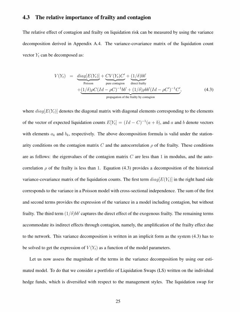
The relative effect of contagion and frailty on liquidation risk can be measured by using the variance

decomposition derived in Appendix A.4. The variance-covariance matrix of the liquidation count

vector Yt can be decomposed as:

V (Yt) = diag[E(Yt)]︸ ︷︷ ︸Poisson

+ CV (Yt)C′︸ ︷︷ ︸

pure contagion

+ (1/δ)bb′︸ ︷︷ ︸direct frailty

+(1/δ)ρC(Id− ρC)−1bb′ + (1/δ)ρbb′(Id− ρC ′)−1C ′︸ ︷︷ ︸propagation of the frailty by contagion

, (4.3)

where diag[E(Yt)] denotes the diagonal matrix with diagonal elements corresponding to the elements

of the vector of expected liquidation counts E[Yt] = (Id − C)−1(a + b), and a and b denote vectors

with elements ak and bk, respectively. The above decomposition formula is valid under the station-

arity conditions on the contagion matrix C and the autocorrelation ρ of the frailty. These conditions

are as follows: the eigenvalues of the contagion matrix C are less than 1 in modulus, and the auto-

correlation ρ of the frailty is less than 1. Equation (4.3) provides a decomposition of the historical

variance-covariance matrix of the liquidation counts. The first term diag[E(Yt)] in the right hand side

corresponds to the variance in a Poisson model with cross-sectional independence. The sum of the first

and second terms provides the expression of the variance in a model including contagion, but without

frailty. The third term (1/δ)bb′ captures the direct effect of the exogenous frailty. The remaining terms

accommodate its indirect effects through contagion, namely, the amplification of the frailty effect due

to the network. This variance decomposition is written in an implicit form as the system (4.3) has to

be solved to get the expression of V (Yt) as a function of the model parameters.

Let us now assess the magnitude of the terms in the variance decomposition by using our esti-

mated model. To do that we consider a portfolio of Liquidation Swaps (LS) written on the individual

hedge funds, which is diversified with respect to the management styles. The liquidation swap for

25

management style k pays 1 USD for each fund of style k that is liquidated in month t. The payoff of

the LS portfolio at month t is e′Yt, where e = (1, 1, ..., 1)′ is a (9, 1) vector of ones. To ensure the

time-invariant diversification, the portfolio of LS has to be appropriately rebalanced when a liquida-

tion occurs. By using the variance decomposition, we can evaluate the percentage of portfolio variance

e′V (Yt)e, due to the underlying idiosyncratic (i.e., management style specific) Poisson shocks, conta-

gion and frailty, respectively. The decomposition is displayed in Table 7.

[Insert Table 7: Decomposition of the variance]

The largest contribution to the portfolio variance comes from the frailty process, either through a direct

effect (64.30%), or through an indirect effect via the contagion network (24.06%). The remaining part

of portfolio variance is explained by the underlying Poisson shocks (6.54%) and the direct contagion

effects (5.10%). Even though the direct effect of contagion is modest, the network plays an important

role in amplifying the effect of the exogenous frailty.

5 The funding liquidity factor

Three types of approaches have been followed in the literature to measure and analyze the funding

liquidity risk and its evolution:

i) The first approach considers directly the refinancing costs. The Treasury-Eurodollar (TED)

spread, equal to the difference between the 3-month Eurodollar LIBOR rate and the 3-month Treasury

bill rate, is such a measure of refinancing cost frequently considered in the literature [see e.g. Gupta,

Subrahmaniam (2000), Boyson, Stahel, Stulz (2010), Teo (2011)].

ii) Alternatively, one could consider a direct measure of market liquidity, such as a bid-ask spread,

and use the link between funding and market liquidity emphasized in Brunnermeier, Pedersen (2009)

[see e.g. Goyenko, Subrahmaniam, Ukhov (2011)].

26

iii) Finally, liquidity is analyzed from its effects on asset prices. In this respect, Vayanos (2004)

suggests to measure the liquidity premium between two assets with similar characteristics, but of

different liquidities. These assets can be for instance thirty-year Treasury bonds just issued (on-the-

run), or issued three months ago. They have the same cash flows, but the on-the-run bonds are much

more liquid [see e.g. Fontaine, Garcia (2012)]. Another example of such assets are the German bonds

(i.e. the bunds) and those issued by the Kreditanstalt fur Wiederaufbau (KfW), a German agency

whose bonds are explicitly guaranteed by the Federal Republic of Germany [see e.g. Gourieroux,

Monfort, Pegoraro, Renne (2013)].

In our paper we follow another approach. Since the hedge funds are often invested in derivatives

and use a high leverage, they can be very sensitive to the funding liquidity risks. Thus, we expect the

common factor in the analysis of hedge fund survival to be a proxy for funding liquidity risk. This

section motivates the funding liquidity risk interpretation of the frailty developed in Subsection 4.2.

We first filter the unobservable factor path. Then, we investigate how this factor is related with other

funding liquidity proxies introduced in the literature.

5.1 Filtering of the factor

The Poisson model with both frailty and contagion is a nonlinear state space model, which requires

adequate methods to filter the unobservable factor. Since the joint process (Y ′t , Ft)′ of observable and

unobservable variables is affine (see Appendix A), the Bates filter [Bates (2006)] might be used to

update the conditional Laplace (or Fourier) transform of the filtering distribution. However, the im-

plementation of the Bates filter requires, at each iteration, the evaluation of a numerical integral of

dimension equal to the number of observable variables. In our model, the vector of observations (the

liquidation counts) is of dimension nine, which makes the implementation of the Bates filter numer-

ically unfeasible. In the online supplementary material we build on the insight of Bates (2006) and

27

propose a new filter for our model, which takes advantage of the affine property of the ARG frailty dy-

namics, but requires only a few one-dimensional numerical integrals to be computed at each iteration.

The filter is based on the idea of approximating any conditional distribution of the frailty given the

available information by means of a distribution in the gamma family (see the online supplementary

material for a description of, and a comparison with, alternative filtering approaches). The filtered path

of the frailty is displayed in Figure 10.

[Insert Figure 10: Filtered path of the frailty]

The frailty features a rather stable path between 1996 and 2006, with spikes at the end of 2001 (the

9/11 terrorist attack), the end of 2002 (the market confidence crisis due to the internet bubble), ... The

frailty path features an upward trend over the years 2007 and 2008 (the recent financial crisis), and

decreases rapidly afterwards.

5.2 The factor interpretation

The TED spread and the VIX are commonly used as measures of capital availability in the economy

[see e.g. Goyenko (2012)]. As already mentioned, the TED spread is a measure of the refinancing cost

on the clearing houses. It is introduced to capture a part of the rollover funding liquidity risk. The

VIX is a weighted average of the implied volatility in the S&P index options. This index measures the

aggregate volatility of the stock market as well as the price of this volatility. In our framework, it is

introduced to capture the magnitude and the cost of leverage. Ang, Gorovyy, van Inwegen (2011) find

that the dynamics of the HF net leverage (i.e., the difference between short and long positions) and

gross leverage (i.e., the sum of these positions) are explained by the VIX and the TED. Adrian, Shin

(2010) report similar findings for other financial intermediaries. The VIX is also introduced to capture

the cost of leverage, i.e., the margin funding liquidity risk. Indeed, for listed derivatives, but also for

28

OTC derivatives, the margin calls depend on the volatility of the underlying index (and are independent

of the riskiness of the fund). Thus, an increase of the volatility, proxied by the VIX, implies an increase

of the margin calls and an increase of the cost of leverage. Moreover, in crisis periods HF managers

turn to VIX futures for volatility hedging and their short positions on VIX futures were for instance so

extreme on February 27, 2013, that the market was close to a significant squeeze. The margin calls on

VIX futures are directly written on the VIX itself. The time series of the TED spread and the VIX are

displayed in Figure 11. The data are obtained from the Federal Reserve Board’s website for the TED

spread, and from the Chicago Board Options Exchange (CBOE) website for the VIX.

[Insert Figure 11: Observable liquidity indicators]

We estimate the regression:

Ft = I(V IXt ≤ c) (β1 + β2TEDt + β3TEDLt + β4V IXt + β5V IXLt + β6SPRt) (4.4)

+I(V IXt > c) (γ1 + γ2TEDt + γ3TEDLt + γ4V IXt + γ5V IXLt + γ6SPRt) + et,

where the explained variable Ft is the filtered value of the frailty. In addition to the current values of the

TED spread and the VIX, the regression includes lagged observations via the average value of the TED

spread in the previous quarter (TEDL) and the average value of the VIX in the previous 12 months

(VIXL), to potentially capture the impacts of the associated innovations. The regression also includes

the spread SPR between the BAA and AAA yields from the FRED database at the Federal Reserve

Bank of St. Louis (see Figure 11, lower panel). It is often stated that part of this spread is unrelated to

credit risk, and it is due to the lower liquidity of the corporate bonds in the more risky rating classes.

While the empirical literature focuses mostly on linear relationships between the unobservable factor

and the observed explanatory variables, we expect to detect nonlinear effects. Indeed, it is widely

believed that hedge funds provide liquidity to the markets, especially to markets of assets with high

29

degree of information asymmetry [see e.g. Agarwal, Fung, Loon, Naik (2007), Brophy, Ouimet,

Sialm (2009)]. However, this occurs in the standard situation of reasonable funding liquidity costs.

In this “good equilibrium”, the hedge funds provide liquidity and are invested in rather illiquid assets

with high leverage. But, as noted in Ben-David, Franzoni, Moussawi (2012), when the refinancing

costs increase, hedge funds reallocate their portfolios, reduce their equity holdings and try to diminish

their leverage in order to anticipate the consequences of possible outflows. In this “bad equilibrium”,

the hedge funds are liquidity seekers. This double equilibrium is captured by the threshold on the

VIX, with the estimated monthly percentage value c = 25. We use a switching regime regression by

allowing for different coefficient values in the low and high volatility regimes. The estimates of the

coefficients in regression (4.4), as well as in some restricted specifications, are displayed in Table 8.

[Insert Table 8: Regression of the frailty on observable variables]

The estimated regressions show that a large fraction of the common factor (i.e. about 70%) is explained

by the proxies for funding liquidity risk introduced in the specifications. The coefficient of TED is

statistically significant (at the 1% level) and larger in the “bad equilibrium”, while in the “good equi-

librium” the lagged value TEDL has a larger effect. The effect of the volatility index passes through

the lagged value VIXL, which has a negative and statistically significant coefficient. This negative

effect of VIXL is more pronounced in the “bad equilibrium”. The negative regression coefficient for

the lagged VIX has to be interpreted in relation with the interaction between VIX and TED. 10 Indeed,

when we regress the frailty on a constant, VIX and VIXL, we find a positive coefficient on the current

VIX, and a negative coefficient of about the same magnitude on the lagged VIX. Thus, the short term

overreaction to a shock to the VIX disappears almost completely in the long term. In other words, the

frailty reacts to the innovations in the VIX. When the TED and its lagged values are included in the

regression, the short term effect of VIX is captured by the TED, and the associated regression coeffi-

10The correlation between VIX and TED is 0.33 in the low volatility regime, and 0.57 in the high volatility regime.

30

cient becomes statistically non-significant. Finally, we observe that the marginal effect of the spread

SPR is smaller in the high volatility regime.

Even if observable proxies for the funding liquidity risk, such as the TED spread and the VIX, can

explain a substantial part of the frailty effect, Table 8 shows that the frailty is not entirely captured by

these observable proxies. This finding highlights the usefulness of including an unobservable common

factor in the liquidation intensity specification. By identifying, a priori, the systematic risk factor

with some observable variables, we would implicitly disregard the risk associated with the difference

between the frailty and the observable proxies.

6 Stress-tests

The estimated model with dynamic frailty and contagion can be used for portfolio management of

a fund of funds, and computation of reserves, etc. In this section, we illustrate how to implement

the prediction of future liquidation counts and the stress-tests for liquidation risk. We consider a

portfolio of HF with fixed style sizes and compare the distribution of the future liquidation counts in

the unstressed and stressed situations. The future counts are subject to a double uncertainty, that is the

drawing of the idiosyncratic risks in the Poisson conditional distribution, and the stochastic evolution

of the exogenous dynamic frailty. The analysis in the unstressed situation corresponds to the prediction

of any (nonlinear) function of the liquidation counts and serves as a benchmark. In the conditioning

set, the unobservable current value Ft of the frailty is replaced by the filtered value (see Section 5.1).

The stress can be designed in the following ways:

i) We can stress the current factor value by setting Ft = qα in the conditioning set, where qα is the

quantile of the estimated stationary distribution of the frailty Ft at level α. By choosing α = 95%, or

99%, we consider an extreme scenario with a large transitory shock to the underlying funding liquidity

risk factor at month t.

31

ii) Alternatively, we can change some parameters values, by either “increasing” the matrix of

contagion C, or by increasing the value of the frailty persistence parameter ρ. This stress scenario will

increase the liquidation risks by amplifying the impact of the exogenous shock by contagion, and by

introducing serial clustering in the exogenous shocks, respectively.

At month t, the stress scenario is characterized by the observed liquidation counts and the possi-

bly stressed values of the factor in month t and the parameter values. Next, the future paths of both

the factor and the liquidation counts could be simulated conditional on this information and used to

compute the conditional distribution of the liquidation counts at any horizon of interest. In particular,

we focus on the term structures of the expected liquidation counts, and of the volatility and overdis-

persion of these counts. Actually, these term structures can be derived in closed form in our model

by using the exponential affine property of the joint process of frailty and liquidation counts (see the

supplementary material). Our stress test analysis is dynamic, as it fully accounts for both liquidation

counts and the exogenous frailty dynamics. Therefore, it sharply differs from the stress test analysis

in models with time-varying observable variables, in which a crystallized scenario for the future factor

path is assumed. Such a stress test would disregard the liquidation risk dependence induced by the

exogenous factors and would generally undervaluate the future risk.

We consider three sets of stress scenarios:

S.1: The current factor value Ft is increased from the filtered value to the 95% quantile of the his-

torical distribution. The parameter values correspond to the estimates of Section 4.2. By con-

ditioning on an extreme event on the current value of the systematic risk factor, the expected

liquidation counts are in line with the measures for systemic risk such as the CoVaR [Adrian,

Brunnermeier (2011)], or the marginal expected shortfall [Acharya et al. (2010)]. The main

difference is in the definition of the conditioning set including the unobservable factor and the

observable liquidation counts, instead of including the return of a market portfolio.

32

S.2: The contagion matrix is changed from C to 2C, where C is the estimate of Section 4.2. The

other parameter values are kept constant and equal to the estimates of Section 4.2. The current

factor value Ft is set equal to the filtered value.

S.3: The frailty autocorrelation is increased from ρ = 0.74 (corresponding to the estimate in Section

4.2) to ρ = 0.90. The other parameter values are kept constant and equal to the estimates of

Section 4.2. The current factor value Ft is set equal to the filtered value.

For all stress scenarios, the filtered value of the frailty and the vector of observed liquidation counts

in the conditioning set correspond to the last month of the sample, i.e. June 2009. The category sizes

correspond to this date as well. In Figures 12, 13 and 14 we display for the nine management styles

the impact of stress scenarios S.1, S.2 and S.3, respectively, on the term structures of the conditional

expectations of liquidation counts. 11

[Insert Figure 12: Term structure of expected liquidation counts when stressing the current factor value]

[Insert Figure 13: Term structure of expected liquidation counts when stressing the contagion matrix]

[Insert Figure 14: Term structure of expected liquidation counts when stressing the frailty persistence]

In each figure, the squares represent the term structures of the expected liquidation counts before

stress, that are the same in each scenario. As the horizon increases, the term structure converges to the

unconditional expectation of the liquidation count, for each management style. The unstressed term

structures are upward sloping since the current month, i.e. June 2009, corresponds to a period with

few liquidation events in any management style and a small frailty value compared to the historical

average. The circles represent the term structures of the expected liquidation counts after the shock.

We observe that the three types of shocks have very different effects on the term structures. The shock

11Figures with the term structures of conditional volatility and overdispersion of liquidation counts are provided in thesupplementary material.

33

to the current factor value in stress scenario S.1 is a transitory funding liquidity shock, with different

impacts in the short run with respect to the management style (see Figure 12). Its effect decays rather

quickly and disappears after about 12 months. The results of these stress tests are compatible with the

liquidity interpretation of the unobservable factor. We observe an immediate effect of the shock on

the highly exposed strategies of the Long/Short Equity Hedge management style, whereas the effect

is clearly lagged, and mainly due to contagion, for the Fixed Income Arbitrage strategies featuring

small factor betas (see Table 4). The magnitude of the impact on the term structure depends on the

conditioning information, i.e. on the liquidation counts at the month of the stress. In stress scenario

S.2, the change in the contagion matrix is a permanent shock. In Figure 13, there is no important effect

in the short run, but the long run behaviors of the models with and without the shock in the contagion

matrix significantly differ for all styles, except for Global Macro. Indeed, the elements in the row of

the estimated contagion matrix (Table 5) for that management style are zero. We conclude that there

is no significant contagion effect impacting the Global Macro style. Therefore, the stress in scenario

S.2 is irrelevant for the distribution of liquidation counts in that management style. Finally, when the

frailty persistence parameter is shocked in stress scenario S.3, we observe an increase in the time at

which the long run expected values of the liquidation counts are attained (Figure 14).

A large part of the literature on financial contagion applied to asset returns defines contagion as

revealed by an increased correlation of asset returns during crisis periods [see e.g. King, Wadhwani

(1990)]. Then, the idea is to test for significant changes in some parameters between the crisis and

non-crisis periods [see e.g. Forbes, Rigobon (2002)]. The above stress-tests analysis shows that there

exist different ways to obtain extreme liquidation counts in some months. This can be due to an

extreme exogenous shock possibly amplified by contagion. It can also be due to a standard exogenous

shock and a significant change in the contagion matrix. These two situations are clearly different.

In the first case, we get an “exogenous crisis” and this exogenous crisis can arise without modifying

34

the contagion matrix C, that is, the speed of propagation of the shocks. In the second case, there

is a change in the structure and speed of contagion, which is more in line with the above mentioned

financial literature. Such a change can be due to either a change in the behaviour of the fund managers,

or of the regulator for systemic risk. 12 To summarize, the model considered in this paper provides

a framework to highlight that the policy maker and the regulator may have to distinguish between

exogenous crises, due to exogenous shocks, and endogenous crises, due to changes in the contagion

matrix. To diminish the probability of an exogenous crisis, the policy maker and the regulator have to

control the extreme exogenous risks, that is, the distribution of factor Ft. As an illustration let us recall

the example of the Asian flu. In order to control the exogenous risk, the authorities in charge of health

supervision will reduce the population of birds. In order to diminish the probability of endogenous

crisis, the authorities would try to limit the contacts between humans. The usual practice of stress tests

is to consider only the exogenous shocks with a given contagion scheme, and to define as carefully

as possible the sources of the shocks. For the analysis of systemic risk, it is more relevant to shock

directly the underlying common risk factor instead of introducing shocks to the idiosyncratic risks of

each management style hidden in the Poisson (conditional) distribution. By selecting the factor we

introduce a common shock to all management styles with different weights given by the frailty beta

coefficients. As the policy maker and the regulator do not have models with frailty and contagion at

hand, they have never implemented stress testing to the contagion scheme itself. Nevertheless, during

the crisis, some regulators have imposed a change of the contagion scheme, for instance by allowing

to isolate a part of the hedge funds portfolios invested in illiquid assets into the so-called side pockets.

Let us now analyse the dynamics of the stress effects over a given horizon. We focus on the stress

to the current factor value similarly as in scenario S.1, and at the one-month horizon.

[Insert Figure 15: Time series of prediction and stress tests for liquidation rates]

12Time variation in the contagion matrix could be made endogenous in the model. Such an extension is beyond thescope of this paper.

35

In Figure 15 we display four time series for each management style: i) The time series of the condi-

tional expected liquidation rate over the period from January 1996 to June 2009. In each month, the

conditioning information corresponds to the filtered value Ft of the frailty and the observed liquidation

counts Yt. ii) The time series of the conditional 95 percentile of the liquidation rate, with the same

conditioning information as in the previous series. iii) The time series of the conditional 95 percentile

of the liquidation rate, with the conditioning information corresponding to the observed liquidation

counts and a stressed value of the frailty. This stressed value is the 95 percentile of the conditional dis-

tribution of the frailty given the current filtered value Ft. iv) The time series of the realized liquidation

rate. We focus on the liquidation rate, instead of the liquidation counts, to eliminate the effect of the

time-varying sizes of the management styles. Moreover, the liquidation rate parallels the portfolio de-

fault probability usually considered in credit risk analysis. 13 The series of the conditional expectation

and conditional quantile in i) and ii) provide the predictions of the mean and an extreme value, re-

spectively, of the one-month-ahead liquidation rate. In particular, the conditional quantile corresponds

to the Value-at-Risk (VaR) measure, and serves as a basis to compute the reserves. The difference

between the conditional quantile and the conditional expectation is the analog of the economic capital.

The use of the current filtered value of the frailty in the conditioning information corresponds to an un-

stressed situation. To get a stressed value of the VaR, we increase the frailty value in the conditioning

set from the filtered value to the 95 percentile of the conditional distribution given this filtered value.

The stressed factor value is defined with respect to the conditional distribution, and not the historical

distribution, in order to ensure that the stressed factor value is an extreme scenario compared to the

current environment also during a crisis period. The difference between the stressed and unstressed

conditional quantiles corresponds to an additional reserve, that is, a second capital buffer.

In Figure 15 the series of conditional quantiles vary over time and increase substantially during the

13The portfolio loss is proportional to the portfolio default frequency, if the portfolio has uniform exposures and therecovery rate, assumed independent of the default event, can be replaced by its expectation, that is, one minus the expectedloss given default.

36

recent financial crisis for most management styles, pointing to the higher liquidation risk in this period.

The panels show that the increase of reserves (VaR and stressed VaR) based on our model starts gradu-

ally from the end of the first quarter of 2007, that is, some months before the freezing announcements.

The dates at which this increase starts differ by one or two months across the management styles, due

to the contagion effect. This rather early increase of the need for reserves is due to the introduction

of the common frailty in the model. This frailty captures the preliminary effect of the crisis once a

first management style is impacted, and is then transmitted to the other management styles. A model

without dynamic frailty would increase the reserves once a significant number of styles have been im-

pacted, that would be too late. Thus, our approach is in line with the recent emphasis on the regulation

of systemic factors, especially the smoothing of the reserve increase at the top of the cycle in order to

diminish the procyclical effect of the regulation on the required capital [Basel Committee on Banking

Supervision (2010)]. In Figure 15, we also observe that the unstressed conditional quantile admits a

coverage close to the nominal one, with occurrences of a realized liquidation rate above the conditional

quantile in line with the 5% nominal probability. The increase in the conditional quantile due to the

stress to the current factor value is rather constant in time. For instance, it is equal to about 0.02 for

the Convertible Arbitrage hedge funds. The realized liquidation rate never exceeds the stressed condi-

tional quantile in our sample. The series of unstressed and stressed predictions for the Global Macro

hedge funds are smoother than for other management styles, since the Global Macro style features a

small sensitivity to the dynamic frailty and is not impacted by significant contagion effects (see Tables

4 and 5).

7 Concluding remarks

In this paper we develop a new methodology to analyse the dynamics of liquidation risk dependence

in the hedge fund industry. The autoregressive Poisson model with dynamic frailty is especially ad-

37

vantageous as it allows for distinguishing the effect of the exogenous shocks, which affect directly the

liability component of the balance sheet, from the endogenous contagion effects, which pass through

the asset component. The common factor, the sensitivities to this factor, and the contagion scheme

can all be interpreted in terms of the liquidity risks. The underlying factor is related nonlinearly to the

standard proxies of rollover and margin funding liquidity risks with two endogenous regimes. In the

first regime, when the aggregate funding liquidity is not tight, the hedge funds are liquidity providers,

while in the second regime, when the aggregate funding liquidity is tight, hedge funds become liquid-

ity seekers. The sensitivities to the factor represent the funding liquidity risk exposures of the different

management styles and are linked with the redemption frequencies and gate management by the fund

managers. Finally, the causal scheme captures a part of the spiral effect highlighted in Brunnermeier,

Pedersen (2009), in which market liquidity and funding liquidity are mutually reinforcing, with a

shock to one management style propagating into the others. Only a specification with both frailty and

contagion allows for performing relevant stress tests. The recent regulation has to define the reserves

to cover extreme systematic risks. To do that the regulator has to stress the systematic factor without

stressing the hedge fund specific risk factors, and to account properly for contagion phenomena. That

analysis leads to the term structure of the reserves for different horizons and the identification of the

systematically important management styles.

The frailty and contagion components could also be disentangled in a more general parametric

dynamic framework. For instance, the model can include more than one factor, or the lagged effects of

these factors on the liquidation intensity. In the latter case, the effect of the (multiple) frailty will also

be observed at some lags. Moreover, the model can account for an autoregressive order larger than

one in the past liquidation counts. The relative magnitude of the frailty and contagion components will

depend on the selected number of factors and lags.

It is known that systemic risk can be due to a significant shock to a common factor amplified by

38

the contagion. Models with both frailty and contagion can reveal the main channel of systemic risk,

namely the exogenous shock and/or contagion, and can help develop accurate strategies against sys-

temic crises. In the hedge funds, such an analysis would have to include jointly the market risk, that is

the returns, and the liquidation risk, that is the lifetime variables. In this respect, our work completes

the systemic risk analysis based on returns developed in a series of recent papers including Sadka

(2010), Boyson, Stahel, Stulz (2010), Akay, Seniuz, Yoldas (2011), Brown et al. (2011), Billio et al.

(2012), Bali, Brown, Caglayan (2012), and the analysis of comovements between the cash inflows and

outflows [Sialm, Sun and Zheng (2012)], especially since the common factor for HF liquidation differs

from the factors usually exhibited for HF returns. In such analysis, it would be interesting to study the

causality between liquidation (or distress) events and returns. Indeed, in August 7, 2007, BNP Paribas

has frozen three investment funds, suspending the calculation of their net asset values. The news of

this event is often considered as an initial step in the recent financial crisis, including the market freeze

for liquidity and the failure of Bear Stearn’s or Lehman Brother’s. However, these funds have been

defrozen later on, and not bankrupted. Thus, some distress events can be advanced indicators of losses

of values on other assets. Of course, such joint analysis might be performed for an enlarged perimeter,

including hedge funds, stocks, corporate bonds, but for the reasons mentioned before clearly distin-

guishing the distress events (liquidation, failure, Chapter 11, renegotiation of credits) from the changes

in values. The specification of a joint model for hedge fund returns and endogenous liquidation is an

interesting avenue for future research.

39

References

Acharya, V., Pedersen, L., Philippon, T., and M., Richardson (2010): “Measuring Systemic Risk”,

Working Paper, New York University.

Adrian, T., and M., Brunnermeier (2011): “CoVaR”, Working Paper, Princeton University and Federal

Reserve Bank of New York.

Adrian, T., and H., Shin (2010): “Liquidity and Leverage”, Journal of Financial Intermediation, 19,

418-437.

Agarwal, V., Daniel, N., and N., Naik (2009): “Role of Managerial Incentives and Discretion in Hedge

Fund Performance”, Journal of Finance, 64, 2221-2256.

Agarwal, V., Fung, W., Loon, Y., and N., Naik (2007): “Liquidity Provision in the Convertible Bond

Market: Analysis of Convertible Arbitrage Hedge Funds”, Working Paper.

Ait-Sahalia, Y., Cacho-Diaz, J., and R., Laeven (2010): “Modeling Financial Contagion Using Mutu-

ally Exciting Jump Processes”, Princeton Univ. DP.

Akay, O., Senyuz, Z., and E., Yoldas (2011): “Understanding Hedge Fund Contagion: A Markov-

switching Dynamic Factor Approach”, DP Bentley University.

Allen, F., and D., Gale (2000): “Financial Contagion”, Journal of Political Economy, 108, 1-11.

Anderson, H., and T., Britton (2000): Stochastic Epidemic Models and Their Statistical Analysis.

Lecture Notes in Statistics, Springer.

Ang, A., Gorovyy, S., and G., van Inwegen (2011): “Hedge Fund Leverage”, NBER Working Paper.

Baba, N., and H., Goko (2006): “Survival Analysis of Hedge Funds”, Bank of Japan, DP, 06-E-05.

Bae, K., Karolyi, A., and R., Stulz (2003): “A New Approach to Measuring Financial Contagion”,

Review of Financial Studies, 16, 717-764.

Bali, T., Brown, S., and M., Caglayan (2012): “Systemic Risk and the Cross-Section of Hedge Funds

Returns”, Journal of Financial Economics, 106, 114-131.

Baquero, G., Horst, J., and M., Verbeek (2005): “Survivor, Look-Ahead Bias and the Performance of

Hedge Funds”, Journal of Financial and Quantitative Analysis, 40, 493-518.

Basel Committee for Banking Supervision (2010): “Guidance for National Authorities Operating the

Countercyclical Capital Buffer”, Consultative Document, Bank of International Settlements, Basel.

Bates, D. (2006): “Maximum Likelihood Estimation of Latent Affine Processes”, Review of Financial

Studies, 19, 909-965.

Bekaert, G., Harvey, C., and A., Ng (2005): “Market Integration and Contagion”, Journal of Business,

78, 1-31.

40

Ben-David, I., Franzoni, F., and R., Moussawi (2012): “Hedge Fund Stock Trading in the Financial

Crisis of 2007-2009”, Review of Financial Studies, 25, 1-54.

Billio, M., Getmansky, M., Lo, A., and L., Pellizzon (2012): “Econometric Measures of Correlation

and Systemic Risk in the Finance and Insurance Sectors”, Journal of Financial Economics, 104, 535-

539.

Boyson, N. (2010): “Implicit Incentives and Reputational Hedging by Hedge Fund Managers”, Jour-

nal of Empirical Finance, 17, 283-299.

Boyson, N., Stahel, C., and R., Stulz (2010): “Hedge Fund Contagion and Liquidity Shocks”, Journal

of Finance, 65, 1789-1816.

Brophy, D., Ouimet, P., and C., Sialm (2009): “Hedge Funds as Investors of Last Resort?”, Review of

Financial Studies, 22, 541-574.

Brown, S., Goetzmann, W., and B., Liang (2004): “Fees on Fees in Funds of Funds”, Journal of

Investment Management, 3, 39-56.

Brown, S., Goetzmann, W., and J., Park (2001): “Careers and Survival Competition and Risks with

Hedge Fund and CTA Industry”, Journal of Finance, 56, 1869-1886.

Brown, S., Hwang, I., In, F., and T., Kim (2011): “Systemic Risk and Cross-Sectional Hedge Fund

Returns”, Working Paper.

Brunnermeier, M., and L. H., Pedersen (2009): “Market Liquidity and Funding Liquidity”, Review of

Financial Studies, 22, 2201-2238.

Cameron, A., and P., Trivedi (1998): Regression Analysis of Count Data, Cambridge University Press,

Cambridge.

Cappe, O., Moulines, E., and T., Ryden (2005): Inference in Hidden Markov Models, Springer Verlag.

Carlson, M., and J., Steinman (2008): “Market Conditions and Hedge Fund Survival”, Federal Reserve

Board, Washington, FEDS Working Paper 2008-28.

Carrasco, M., Chernov, M., Florens, J.-P., and E., Ghysels (2007): “Efficient Estimation of General

Dynamic Models with a Continuum of Moment Conditions”, Journal of Econometrics, 140, 529-573.

Chan, N., Getmansky, M., Haas, S. and A., Lo (2007): “Systemic Risk and Hedge Funds”, in The

Risks of Financial Institutions, ed. by M., Carey and R., Stulz, University of Chicago Press, 235-338.

Cox, D. (1972): “Regression Models and Life Tables”, Journal of the Royal Statistical Society, Series

B, 34, 187-220.

Cox, J., Ingersoll, J., and S. Ross (1985): “A Theory of the Term Structure of Interest Rates”, Econo-

metrica, 53, 385-407.

41

Czado, C., Delwarde, A., and M., Denuit (2005): “Bayesian Poisson Log-bilinear Mortality Projec-

tions”, Insurance: Mathematics and Economics, 36, 260-284.

Darolles, S., and C., Gourieroux (2014): “The Effects of Management and Provision Accounts on

Hedge Fund Returns. Part 1: High Water Mark Allocation Scheme; Part 2: Loss Carry Forward

Scheme”, in Advances in Intelligent Systems and Computing, 251, V. Huyun et al. eds, Springer,

23-46 and 47-62.

Darolles, S., Gourieroux, C., and J., Jasiak (2006): “Structural Laplace Transform and Compound

Autoregressive Models”, Journal of Time Series Analysis, 27, 477-503.

Diamond, D., and P., Dybvig (1983): “Bank Runs, Deposit Insurance, and Liquidity”, Journal of

Political Economy, 91, 401-419.

Duffie, D., Eckner, A., Horel, G., and L., Saita (2009): “Frailty Correlated Default”, Journal of Fi-

nance, 64, 2089-2183.

Duffie, D., Filipovic, D., and W., Schachermayer (2003): “Affine Processes and Applications in Fi-

nance”, Annals of Applied Probability, 13, 984-1053.

Dungey, M., Fry, R., Gonzalez-Hermosillo, B., and V., Martin (2005): “Empirical Modeling of Con-

tagion: A Review of Methodologies”, Quantitative Finance, 5, 9-24.

Egloff, D., Leippold, M., and P., Vanini (2007): “A Simple Model of Credit Contagion”, Journal of

Banking and Finance, 31, 2475-2492.

Eichengreen, B., Rose, A., and C., Wyplosz (1996): “Contagious Currency Crises: First Tests”, Scan-

dinavian Journal of Economics, 98, 463-484.

Fontaine, J.-S., and R., Garcia (2012) : “Bond Liquidity Premia”, Review of Financial Studies, 25,

1207-1254.

Forbes, K., and R., Rigobon (2002): “No Contagion, Only Interdependence: Measuring Stock Market

Co-Movements”, Journal of Finance, 57, 2223-2261.

Gagliardini, P., and C., Gourieroux (2012): “Identification by Laplace Transforms in Panel and Time

Series Models with Unobserved Stochastic Time Effects”, DP CREST.

Gagliardini, P., and C., Gourieroux (2013): “Correlated Risks vs Contagion in Stochastic Transition

Models”, forthcoming in Journal of Economic Dynamics and Control.

Getmansky, M. (2010): “The Life Cycle of Hedge Funds: Fund Flows, Size and Performance”, DP

MIT.

Getmansky, M., Lo, A., and S., Mei (2004): “Sifting Through the Wreckage: Lessons from Recent

Hedge-Fund Liquidations”, Journal of Investment Management, 2, 6-38.

42

Gourieroux, C., Heam, J.-C., and A., Monfort (2012): “Bilateral Exposures and Systemic Solvency

Risk”, Canadian Journal of Statistics, 45, 1273-1309.

Gourieroux, C., and J., Jasiak (2006): “Autoregressive Gamma Process”, Journal of Forecasting, 25,

129-152.

Gourieroux, C., Monfort, A., Pegoraro, F., and J.-P., Renne (2013): “Regime Switching and Bond

Pricing”, forthcoming in Journal of Financial Econometrics.

Goyenko, R. (2012): “Treasury Liquidity and Funding Liquidity: Evidence from Mutual Fund Re-

turns”, DP McGill University.

Goyenko, R., Subrahmaniam, A., and A., Uhkov (2011): “The Term Structure of Bond Market Liquid-

ity and its Implications for Expected Bond Returns”, Journal of Financial and Quantitative Analysis,

46, 111-139.

Gregoriou, G., Lhabitant, F.-S., and F., Rouah (2010): “Survival of Exchange-Listed Hedge Funds”,

Journal of Applied Research in Accounting and Finance, 4, 2-11.

Gupta, A., and M., Subrahmaniam (2000): “An Empirical Investigation of the Convexity Bias in the

Pricing of Interest Rate Swaps”, Journal of Financial Economics, 55, 239-279.

Hansen, L. (1982): “Large Sample Properties of Generalized Method of Moments Estimators”, Econo-

metrica, 50, 1029-1054.

Hansen, L., and K., Singleton (1982): “Generalized Instrumental Variable Estimation of Nonlinear

Rational Expectations Models”, Econometrica, 50, 1269-1286.

Kaplan, E., and P., Meier (1958): “Nonparametric Estimation from Incomplete Observations”, Journal

of the American Statistical Association, 53, 457-481.

Kermack, W., and A., McKendrick (1927): “A Contribution to the Mathematical Theory of Epidemics.

Part I”, Proceedings of the Royal Society A, 115, 700-721. Reprinted in Bulletin of Mathematical

Biology, 53, 33-55.

Kermack, W., and A., McKendrick (1932): “A Contribution to the Mathematical Theory of Epidemics.

Part II”, Proceedings of the Royal Society London, 138, 55-83.

Kermack, W., and A., McKendrick (1933): “A Contribution to the Mathematical Theory of Epidemics.

Part III”, Proceedings of the Royal Society London, 141, 94-112.

King, M., and S., Wadhwani (1990): “Transmission of Volatility Between Stock Markets”, Review of

Financial Studies, 3, 5-33.

Malkiel, B., and A., Saha (2005): “Hedge Funds: Risk and Return”, Financial Analysts Journal, 61,

80-88.

43

Manski, C. (1993): “Identification of Endogenous Social Effects: The Reflection Problem”, Review of

Economic Studies, 60, 531-542.

MSCI (2006): “Hedge Fund Indices: Index Methodology”, Morningstar, Objectives and Guiding Prin-

ciples.

Oakes, D. (1989): “Bivariate Survival Models Induced by Frailties”, Journal of the American Statisti-

cal Association, 84, 487-493.

Patton, A. (2009): “Are “Market Neutral” Hedge Funds Really Market Neutral?”, Review of Financial

Studies, 22, 2495-2530.

Ross, R. (1911): The Prevention of Malaria. John Murray, London.

Sadka, R. (2010): “Liquidity Risk and the Cross Section of Hedge Fund Returns”, Journal of Financial

Economics, 98, 54-71.

Shleifer, A., and R., Vishny (1997): “The Limits of Arbitrage”, Journal of Finance, 52, 35-55.

Sialm, C., Sun, Z., and L., Zheng (2012): “Home Bias and Local Contagion: Evidence From Funds of

Funds”, Working Paper, University of California Irvine.

Teo, M. (2011): “The Liquidity Risk of Liquid Hedge Funds”, Journal of Financial Economics, 100,

24-44.

Upper, C., and A., Worms (2004): “Estimating Bilateral Exposures in the German Interbank Market:

Is There a Danger of Contagion?”, European Economic Review, 48, 827-849.

Vaupel, J., Manton, K., and E., Stallard (1979): “The Impact of Heterogeneity in Individual Frailty on

the Dynamics of Mortality”, Demography, 16, 439-454.

Vayanos, D. (2004): “Flight to Quality, Flight to Liquidity, and the Pricing of Risk”, NBER WP 10327.

44

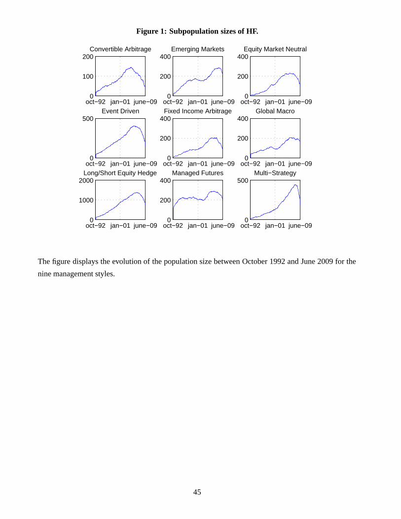
Figure 1: Subpopulation sizes of HF.

oct−92 jan−01 june−090

100

200Convertible Arbitrage

oct−92 jan−01 june−090

200

400Emerging Markets

oct−92 jan−01 june−090

200

400Equity Market Neutral

oct−92 jan−01 june−090

500Event Driven

oct−92 jan−01 june−090

200

400Fixed Income Arbitrage

oct−92 jan−01 june−090

200

400Global Macro

oct−92 jan−01 june−090

1000

2000Long/Short Equity Hedge

oct−92 jan−01 june−090

200

400Managed Futures

oct−92 jan−01 june−090

500Multi−Strategy

The figure displays the evolution of the population size between October 1992 and June 2009 for the

nine management styles.

45

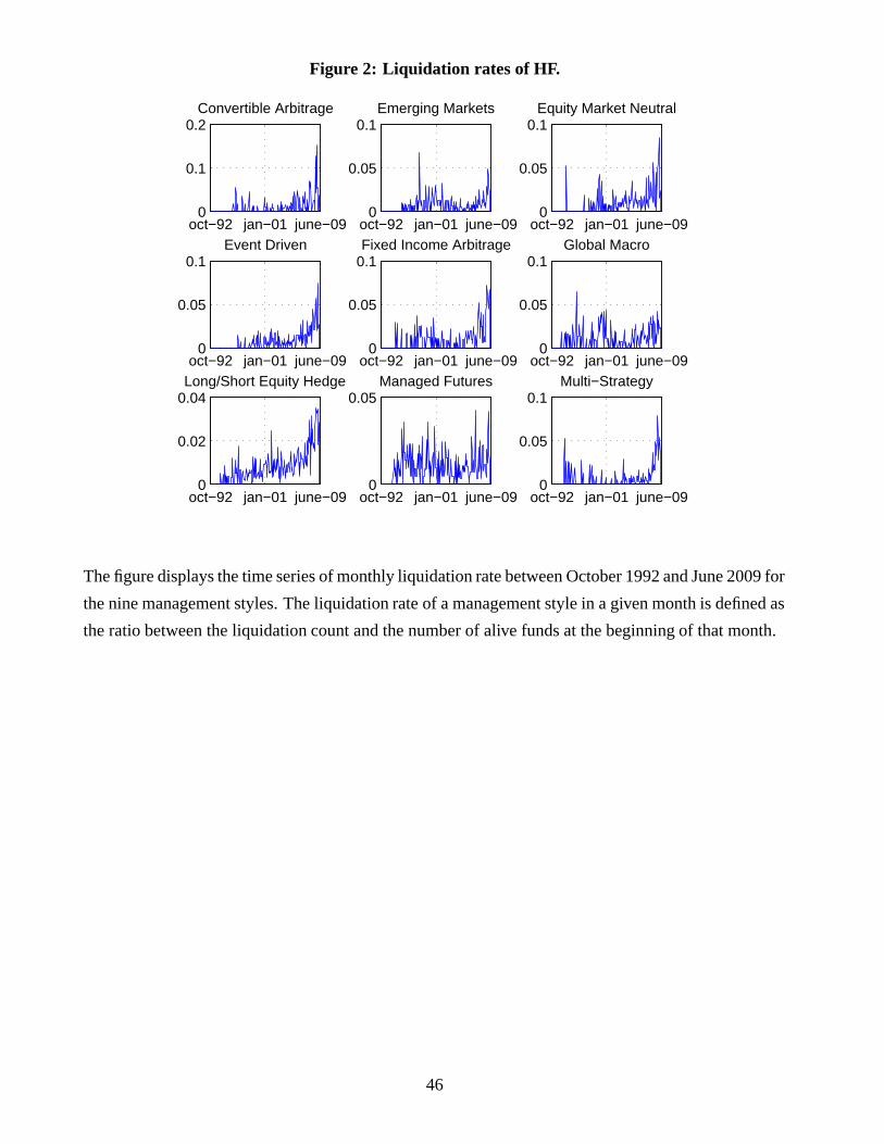
Figure 2: Liquidation rates of HF.

oct−92 jan−01 june−090

0.1

0.2Convertible Arbitrage

oct−92 jan−01 june−090

0.05

0.1Emerging Markets

oct−92 jan−01 june−090

0.05

0.1Equity Market Neutral

oct−92 jan−01 june−090

0.05

0.1Event Driven

oct−92 jan−01 june−090

0.05

0.1Fixed Income Arbitrage

oct−92 jan−01 june−090

0.05

0.1Global Macro

oct−92 jan−01 june−090

0.02

0.04Long/Short Equity Hedge

oct−92 jan−01 june−090

0.05Managed Futures

oct−92 jan−01 june−090

0.05

0.1Multi−Strategy

The figure displays the time series of monthly liquidation rate between October 1992 and June 2009 for

the nine management styles. The liquidation rate of a management style in a given month is defined as

the ratio between the liquidation count and the number of alive funds at the beginning of that month.

46

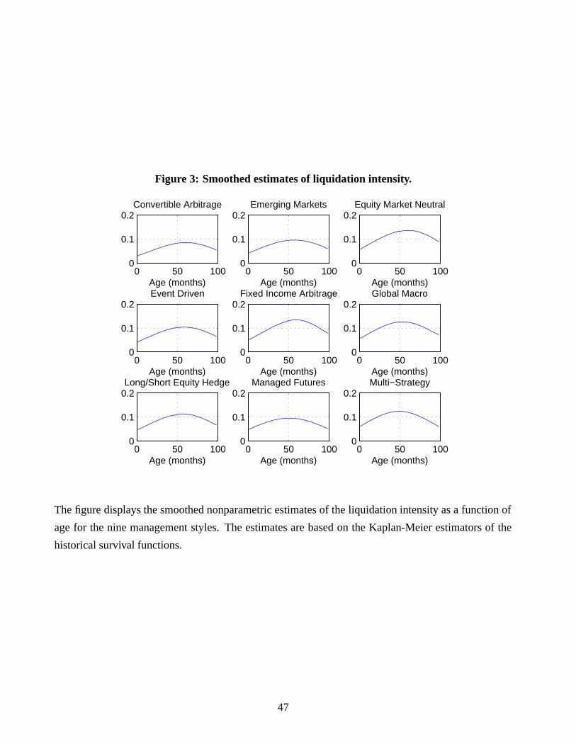
Figure 3: Smoothed estimates of liquidation intensity.

0 50 1000

0.1

0.2Convertible Arbitrage

Age (months)0 50 100

0

0.1

0.2Emerging Markets

Age (months)0 50 100

0

0.1

0.2Equity Market Neutral

Age (months)

0 50 1000

0.1

0.2Event Driven

Age (months)0 50 100

0

0.1

0.2Fixed Income Arbitrage

Age (months)0 50 100

0

0.1

0.2Global Macro

Age (months)

0 50 1000

0.1

0.2Long/Short Equity Hedge

Age (months)0 50 100

0

0.1

0.2Managed Futures

Age (months)0 50 100

0

0.1

0.2Multi−Strategy

Age (months)

The figure displays the smoothed nonparametric estimates of the liquidation intensity as a function of

age for the nine management styles. The estimates are based on the Kaplan-Meier estimators of the

historical survival functions.

47

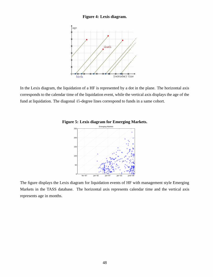
Figure 4: Lexis diagram.

In the Lexis diagram, the liquidation of a HF is represented by a dot in the plane. The horizontal axis

corresponds to the calendar time of the liquidation event, while the vertical axis displays the age of the

fund at liquidation. The diagonal 45-degree lines correspond to funds in a same cohort.

Figure 5: Lexis diagram for Emerging Markets.

fev−87 jan−92 jan−97 jan−03 june−090

50

100

150

200

250Emerging Markets

The figure displays the Lexis diagram for liquidation events of HF with management style Emerging

Markets in the TASS database. The horizontal axis represents calendar time and the vertical axis

represents age in months.

48

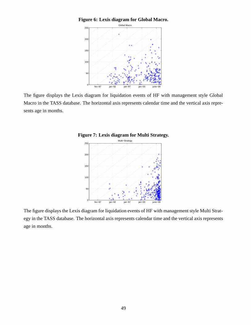
Figure 6: Lexis diagram for Global Macro.

fev−87 jan−92 jan−97 jan−03 june−090

50

100

150

200

250Global Macro

The figure displays the Lexis diagram for liquidation events of HF with management style Global

Macro in the TASS database. The horizontal axis represents calendar time and the vertical axis repre-

sents age in months.

Figure 7: Lexis diagram for Multi Strategy.

fev−87 jan−92 jan−97 jan−03 june−090

50

100

150

200

250Multi−Strategy

The figure displays the Lexis diagram for liquidation events of HF with management style Multi Strat-

egy in the TASS database. The horizontal axis represents calendar time and the vertical axis represents

age in months.

49

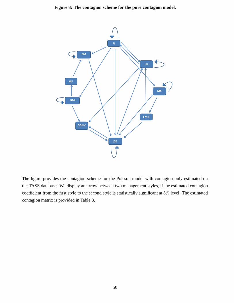
Figure 8: The contagion scheme for the pure contagion model.

FI

LSE

EM

MF

GM

CONV

ED

MS

EMN

The figure provides the contagion scheme for the Poisson model with contagion only estimated on

the TASS database. We display an arrow between two management styles, if the estimated contagion

coefficient from the first style to the second style is statistically significant at 5% level. The estimated

contagion matrix is provided in Table 3.

50

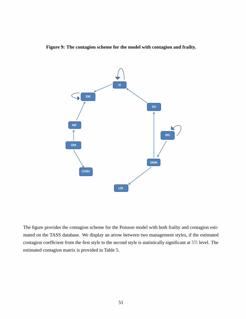
Figure 9: The contagion scheme for the model with contagion and frailty.

FI

LSE

EM

MF

GM

CONV

ED

MS

EMN

The figure provides the contagion scheme for the Poisson model with both frailty and contagion esti-

mated on the TASS database. We display an arrow between two management styles, if the estimated

contagion coefficient from the first style to the second style is statistically significant at 5% level. The

estimated contagion matrix is provided in Table 5.

51

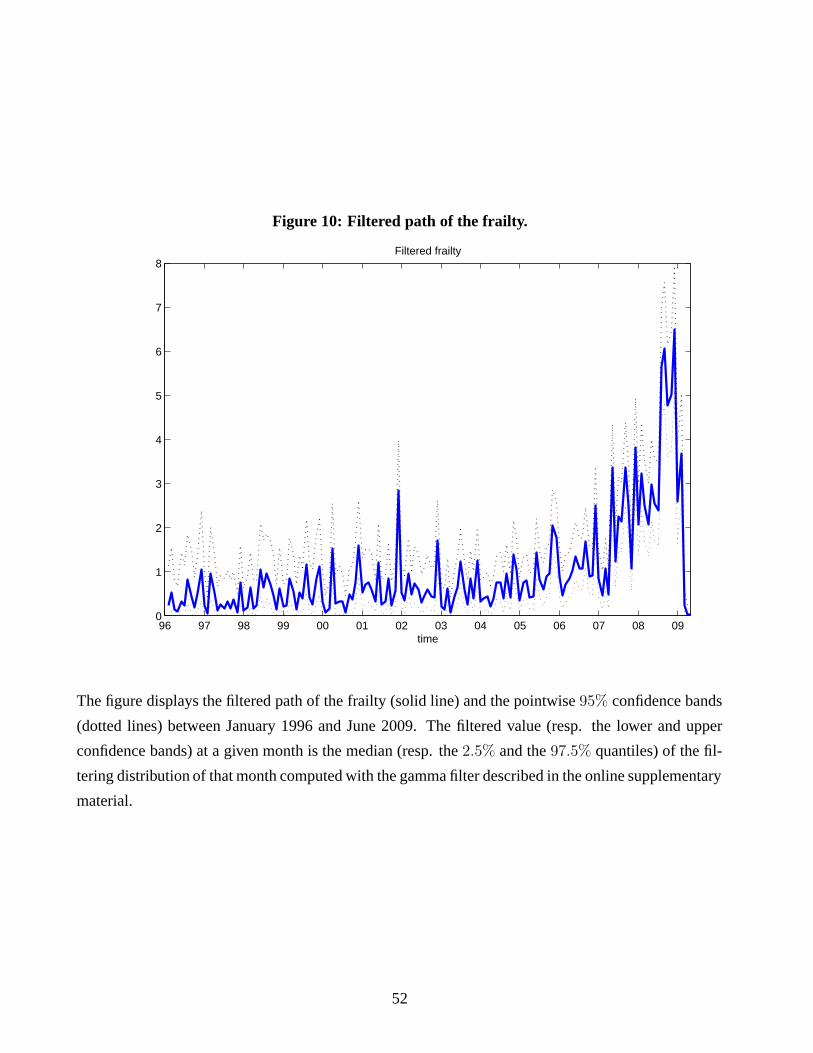
Figure 10: Filtered path of the frailty.

96 97 98 99 00 01 02 03 04 05 06 07 08 090

1

2

3

4

5

6

7

8Filtered frailty

time

The figure displays the filtered path of the frailty (solid line) and the pointwise 95% confidence bands

(dotted lines) between January 1996 and June 2009. The filtered value (resp. the lower and upper

confidence bands) at a given month is the median (resp. the 2.5% and the 97.5% quantiles) of the fil-

tering distribution of that month computed with the gamma filter described in the online supplementary

material.

52

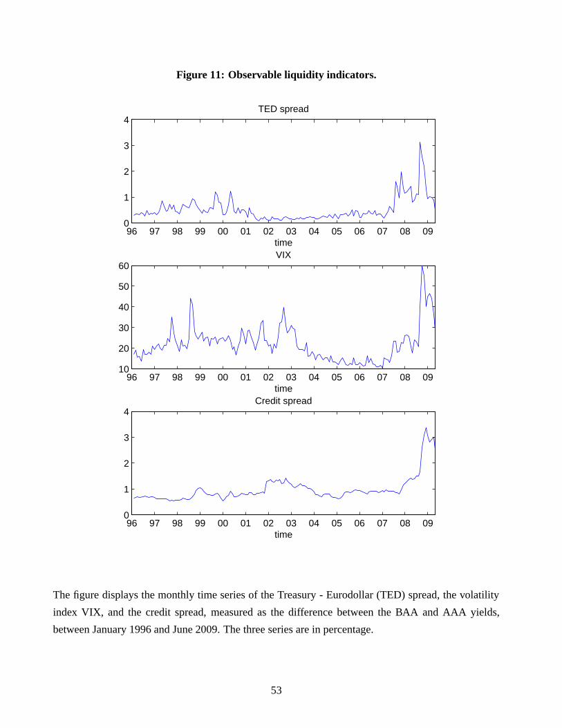
Figure 11: Observable liquidity indicators.

96 97 98 99 00 01 02 03 04 05 06 07 08 090

1

2

3

4TED spread

time

96 97 98 99 00 01 02 03 04 05 06 07 08 0910

20

30

40

50

60VIX

time

96 97 98 99 00 01 02 03 04 05 06 07 08 090

1

2

3

4Credit spread

time

The figure displays the monthly time series of the Treasury - Eurodollar (TED) spread, the volatility

index VIX, and the credit spread, measured as the difference between the BAA and AAA yields,

between January 1996 and June 2009. The three series are in percentage.

53

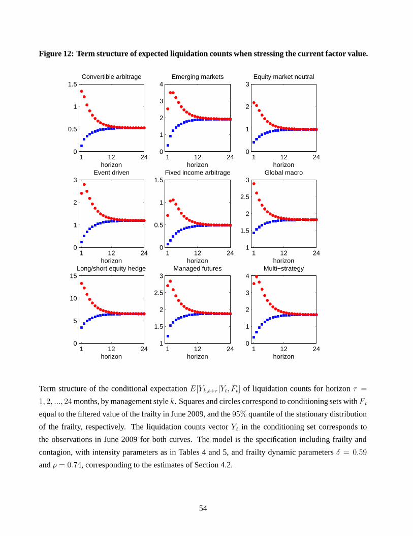
Figure 12: Term structure of expected liquidation counts when stressing the current factor value.

1 12 240

0.5

1

1.5Convertible arbitrage

horizon1 12 24

0

1

2

3

4Emerging markets

horizon1 12 24

0

1

2

3Equity market neutral

horizon

1 12 240

1

2

3Event driven

horizon1 12 24

0

0.5

1

1.5Fixed income arbitrage

horizon1 12 24

1

1.5

2

2.5

3Global macro

horizon

1 12 240

5

10

15Long/short equity hedge

horizon1 12 24

1

1.5

2

2.5

3Managed futures

horizon1 12 24

0

1

2

3

4Multi−strategy

horizon

Term structure of the conditional expectation E[Yk,t+τ |Yt, Ft] of liquidation counts for horizon τ =

1, 2, ..., 24 months, by management style k. Squares and circles correspond to conditioning sets with F t

equal to the filtered value of the frailty in June 2009, and the 95% quantile of the stationary distribution

of the frailty, respectively. The liquidation counts vector Yt in the conditioning set corresponds to

the observations in June 2009 for both curves. The model is the specification including frailty and

contagion, with intensity parameters as in Tables 4 and 5, and frailty dynamic parameters δ = 0.59

and ρ = 0.74, corresponding to the estimates of Section 4.2.

54

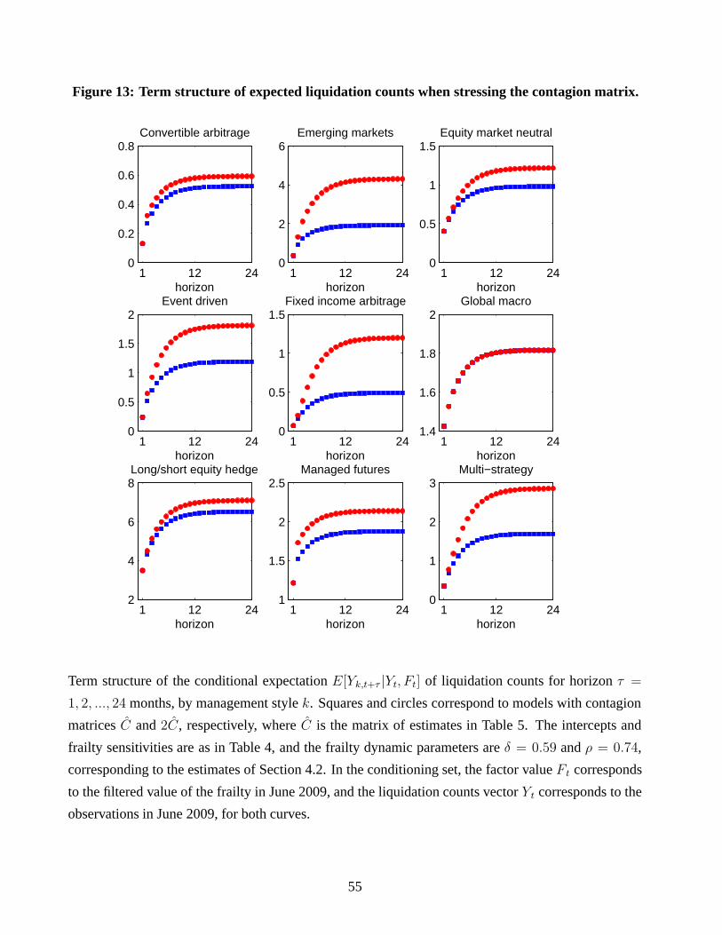
Figure 13: Term structure of expected liquidation counts when stressing the contagion matrix.

1 12 240

0.2

0.4

0.6

0.8Convertible arbitrage

horizon1 12 24

0

2

4

6Emerging markets

horizon1 12 24

0

0.5

1

1.5Equity market neutral

horizon

1 12 240

0.5

1

1.5

2Event driven

horizon1 12 24

0

0.5

1

1.5Fixed income arbitrage

horizon1 12 24

1.4

1.6

1.8

2Global macro

horizon

1 12 242

4

6

8Long/short equity hedge

horizon1 12 24

1

1.5

2

2.5Managed futures

horizon1 12 24

0

1

2

3Multi−strategy

horizon

Term structure of the conditional expectation E[Yk,t+τ |Yt, Ft] of liquidation counts for horizon τ =

1, 2, ..., 24 months, by management style k. Squares and circles correspond to models with contagion

matrices C and 2C, respectively, where C is the matrix of estimates in Table 5. The intercepts and

frailty sensitivities are as in Table 4, and the frailty dynamic parameters are δ = 0.59 and ρ = 0.74,

corresponding to the estimates of Section 4.2. In the conditioning set, the factor value Ft corresponds

to the filtered value of the frailty in June 2009, and the liquidation counts vector Yt corresponds to the

observations in June 2009, for both curves.

55

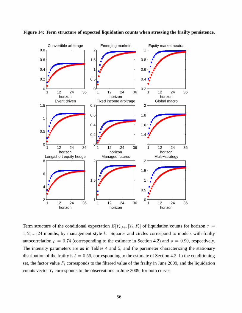
Figure 14: Term structure of expected liquidation counts when stressing the frailty persistence.

1 12 24 360

0.2

0.4

0.6

0.8Convertible arbitrage

horizon1 12 24 36

0

0.5

1

1.5

2Emerging markets

horizon1 12 24 36

0.2

0.4

0.6

0.8

1Equity market neutral

horizon

1 12 24 360

0.5

1

1.5Event driven

horizon1 12 24 36

0

0.2

0.4

0.6

0.8Fixed income arbitrage

horizon1 12 24 36

1.4

1.6

1.8

2Global macro

horizon

1 12 24 362

4

6

8Long/short equity hedge

horizon1 12 24 36

1

1.5

2Managed futures

horizon1 12 24 36

0

0.5

1

1.5

2Multi−strategy

horizon

Term structure of the conditional expectation E[Yk,t+τ |Yt, Ft] of liquidation counts for horizon τ =

1, 2, ..., 24 months, by management style k. Squares and circles correspond to models with frailty

autocorrelation ρ = 0.74 (corresponding to the estimate in Section 4.2) and ρ = 0.90, respectively.

The intensity parameters are as in Tables 4 and 5, and the parameter characterizing the stationary

distribution of the frailty is δ = 0.59, corresponding to the estimate of Section 4.2. In the conditioning

set, the factor value Ft corresponds to the filtered value of the frailty in June 2009, and the liquidation

counts vector Yt corresponds to the observations in June 2009, for both curves.

56

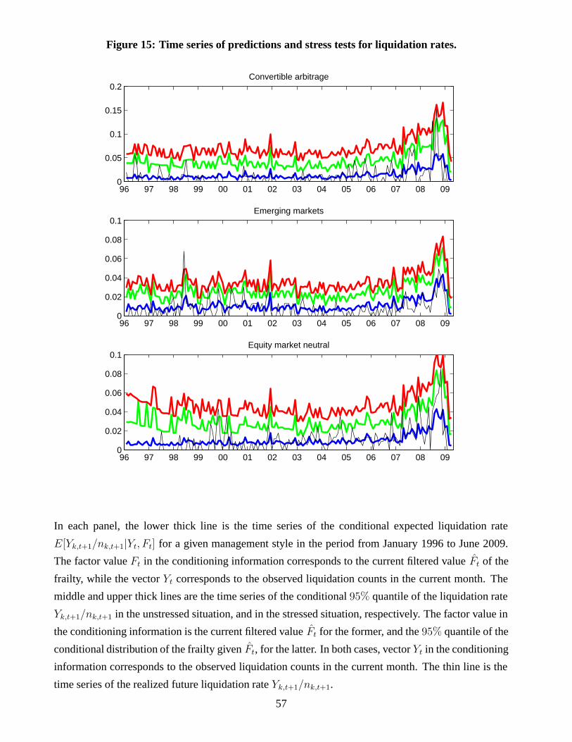
Figure 15: Time series of predictions and stress tests for liquidation rates.

96 97 98 99 00 01 02 03 04 05 06 07 08 090

0.05

0.1

0.15

0.2Convertible arbitrage

96 97 98 99 00 01 02 03 04 05 06 07 08 090

0.02

0.04

0.06

0.08

0.1Emerging markets

96 97 98 99 00 01 02 03 04 05 06 07 08 090

0.02

0.04

0.06

0.08

0.1Equity market neutral

In each panel, the lower thick line is the time series of the conditional expected liquidation rate

E[Yk,t+1/nk,t+1|Yt, Ft] for a given management style in the period from January 1996 to June 2009.

The factor value Ft in the conditioning information corresponds to the current filtered value Ft of the

frailty, while the vector Yt corresponds to the observed liquidation counts in the current month. The

middle and upper thick lines are the time series of the conditional 95% quantile of the liquidation rate

Yk,t+1/nk,t+1 in the unstressed situation, and in the stressed situation, respectively. The factor value in

the conditioning information is the current filtered value Ft for the former, and the 95% quantile of the

conditional distribution of the frailty given Ft, for the latter. In both cases, vector Yt in the conditioning

information corresponds to the observed liquidation counts in the current month. The thin line is the

time series of the realized future liquidation rate Yk,t+1/nk,t+1.

57

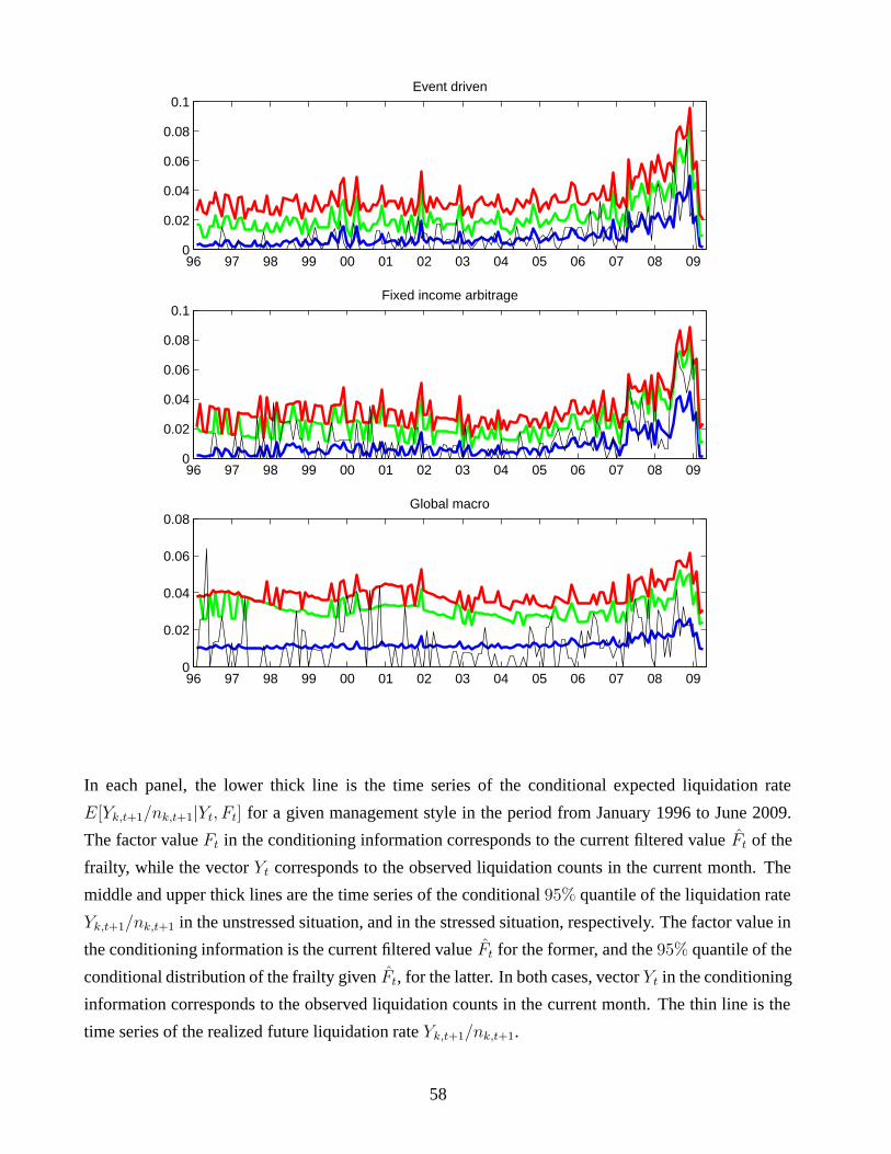
96 97 98 99 00 01 02 03 04 05 06 07 08 090

0.02

0.04

0.06

0.08

0.1Event driven

96 97 98 99 00 01 02 03 04 05 06 07 08 090

0.02

0.04

0.06

0.08

0.1Fixed income arbitrage

96 97 98 99 00 01 02 03 04 05 06 07 08 090

0.02

0.04

0.06

0.08Global macro

In each panel, the lower thick line is the time series of the conditional expected liquidation rate

E[Yk,t+1/nk,t+1|Yt, Ft] for a given management style in the period from January 1996 to June 2009.

The factor value Ft in the conditioning information corresponds to the current filtered value Ft of the

frailty, while the vector Yt corresponds to the observed liquidation counts in the current month. The

middle and upper thick lines are the time series of the conditional 95% quantile of the liquidation rate

Yk,t+1/nk,t+1 in the unstressed situation, and in the stressed situation, respectively. The factor value in

the conditioning information is the current filtered value Ft for the former, and the 95% quantile of the

conditional distribution of the frailty given Ft, for the latter. In both cases, vector Yt in the conditioning

information corresponds to the observed liquidation counts in the current month. The thin line is the

time series of the realized future liquidation rate Yk,t+1/nk,t+1.

58

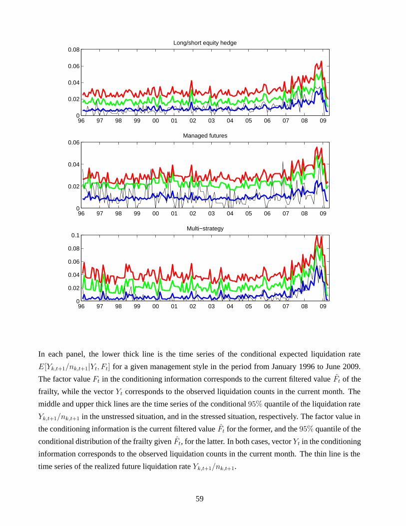
96 97 98 99 00 01 02 03 04 05 06 07 08 090

0.02

0.04

0.06

0.08Long/short equity hedge

96 97 98 99 00 01 02 03 04 05 06 07 08 090

0.02

0.04

0.06Managed futures

96 97 98 99 00 01 02 03 04 05 06 07 08 090

0.02

0.04

0.06

0.08

0.1Multi−strategy

In each panel, the lower thick line is the time series of the conditional expected liquidation rate

E[Yk,t+1/nk,t+1|Yt, Ft] for a given management style in the period from January 1996 to June 2009.

The factor value Ft in the conditioning information corresponds to the current filtered value Ft of the

frailty, while the vector Yt corresponds to the observed liquidation counts in the current month. The

middle and upper thick lines are the time series of the conditional 95% quantile of the liquidation rate

Yk,t+1/nk,t+1 in the unstressed situation, and in the stressed situation, respectively. The factor value in

the conditioning information is the current filtered value Ft for the former, and the 95% quantile of the

conditional distribution of the frailty given Ft, for the latter. In both cases, vector Yt in the conditioning

information corresponds to the observed liquidation counts in the current month. The thin line is the

time series of the realized future liquidation rate Yk,t+1/nk,t+1.

59

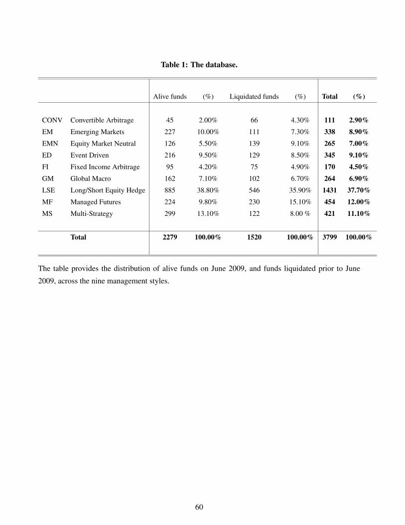
Table 1: The database.

Alive funds (%) Liquidated funds (%) Total (%)

CONV Convertible Arbitrage 45 2.00% 66 4.30% 111 2.90%EM Emerging Markets 227 10.00% 111 7.30% 338 8.90%EMN Equity Market Neutral 126 5.50% 139 9.10% 265 7.00%ED Event Driven 216 9.50% 129 8.50% 345 9.10%FI Fixed Income Arbitrage 95 4.20% 75 4.90% 170 4.50%GM Global Macro 162 7.10% 102 6.70% 264 6.90%LSE Long/Short Equity Hedge 885 38.80% 546 35.90% 1431 37.70%MF Managed Futures 224 9.80% 230 15.10% 454 12.00%MS Multi-Strategy 299 13.10% 122 8.00 % 421 11.10%

Total 2279 100.00% 1520 100.00% 3799 100.00%

The table provides the distribution of alive funds on June 2009, and funds liquidated prior to June

2009, across the nine management styles.

60

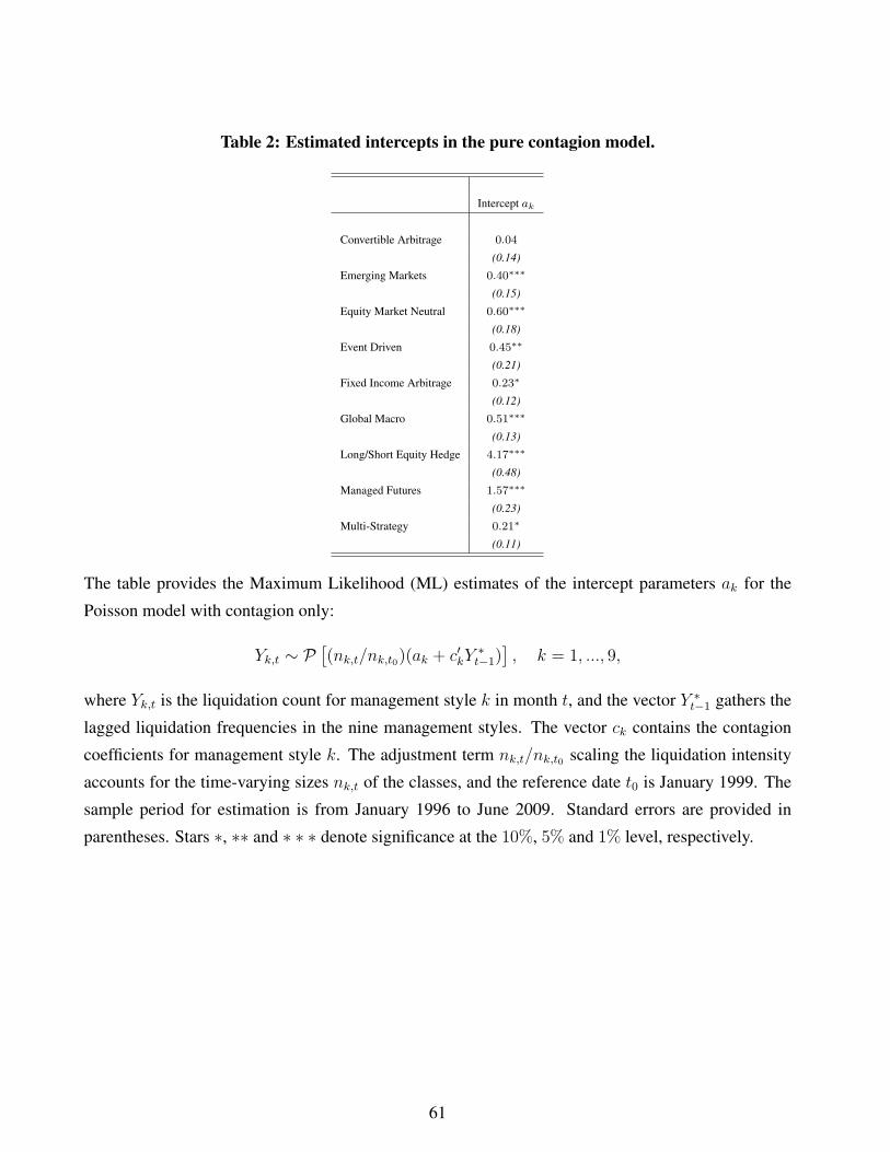
Table 2: Estimated intercepts in the pure contagion model.

Intercept ak

Convertible Arbitrage 0.04

(0.14)

Emerging Markets 0.40∗∗∗

(0.15)

Equity Market Neutral 0.60∗∗∗

(0.18)

Event Driven 0.45∗∗

(0.21)

Fixed Income Arbitrage 0.23∗

(0.12)

Global Macro 0.51∗∗∗

(0.13)

Long/Short Equity Hedge 4.17∗∗∗

(0.48)

Managed Futures 1.57∗∗∗

(0.23)

Multi-Strategy 0.21∗

(0.11)

The table provides the Maximum Likelihood (ML) estimates of the intercept parameters ak for the

Poisson model with contagion only:

Yk,t ∼ P[(nk,t/nk,t0)(ak + c′kY

∗t−1)

], k = 1, ..., 9,

where Yk,t is the liquidation count for management style k in month t, and the vector Y ∗t−1 gathers the

lagged liquidation frequencies in the nine management styles. The vector ck contains the contagion

coefficients for management style k. The adjustment term nk,t/nk,t0 scaling the liquidation intensity

accounts for the time-varying sizes nk,t of the classes, and the reference date t0 is January 1999. The

sample period for estimation is from January 1996 to June 2009. Standard errors are provided in

parentheses. Stars ∗, ∗∗ and ∗ ∗ ∗ denote significance at the 10%, 5% and 1% level, respectively.

61

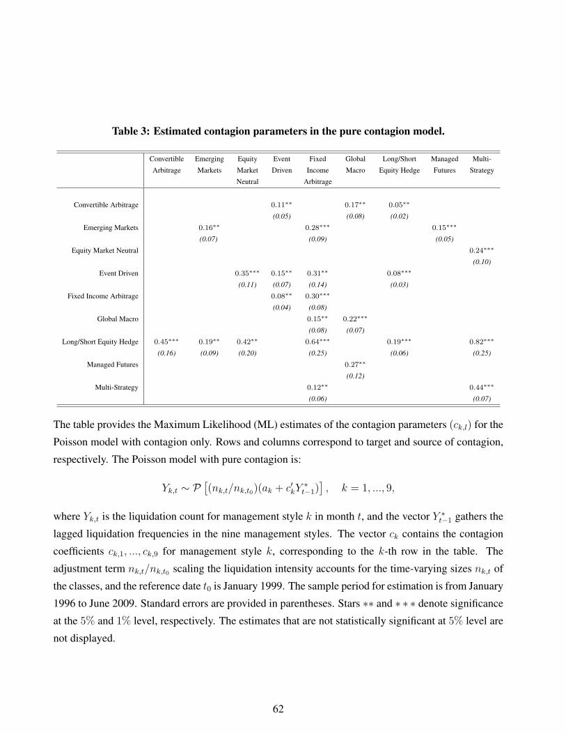
Table 3: Estimated contagion parameters in the pure contagion model.

Convertible Emerging Equity Event Fixed Global Long/Short Managed Multi-

Arbitrage Markets Market Driven Income Macro Equity Hedge Futures Strategy

Neutral Arbitrage

Convertible Arbitrage 0.11∗∗ 0.17∗∗ 0.05∗∗

(0.05) (0.08) (0.02)

Emerging Markets 0.16∗∗ 0.28∗∗∗ 0.15∗∗∗

(0.07) (0.09) (0.05)

Equity Market Neutral 0.24∗∗∗

(0.10)

Event Driven 0.35∗∗∗ 0.15∗∗ 0.31∗∗ 0.08∗∗∗

(0.11) (0.07) (0.14) (0.03)

Fixed Income Arbitrage 0.08∗∗ 0.30∗∗∗

(0.04) (0.08)

Global Macro 0.15∗∗ 0.22∗∗∗

(0.08) (0.07)

Long/Short Equity Hedge 0.45∗∗∗ 0.19∗∗ 0.42∗∗ 0.64∗∗∗ 0.19∗∗∗ 0.82∗∗∗

(0.16) (0.09) (0.20) (0.25) (0.06) (0.25)

Managed Futures 0.27∗∗

(0.12)

Multi-Strategy 0.12∗∗ 0.44∗∗∗

(0.06) (0.07)

The table provides the Maximum Likelihood (ML) estimates of the contagion parameters (ck,l) for the

Poisson model with contagion only. Rows and columns correspond to target and source of contagion,

respectively. The Poisson model with pure contagion is:

Yk,t ∼ P[(nk,t/nk,t0)(ak + c′kY

∗t−1)

], k = 1, ..., 9,

where Yk,t is the liquidation count for management style k in month t, and the vector Y ∗t−1 gathers the

lagged liquidation frequencies in the nine management styles. The vector ck contains the contagion

coefficients ck,1, ..., ck,9 for management style k, corresponding to the k-th row in the table. The

adjustment term nk,t/nk,t0 scaling the liquidation intensity accounts for the time-varying sizes nk,t of

the classes, and the reference date t0 is January 1999. The sample period for estimation is from January

1996 to June 2009. Standard errors are provided in parentheses. Stars ∗∗ and ∗ ∗ ∗ denote significance

at the 5% and 1% level, respectively. The estimates that are not statistically significant at 5% level are

not displayed.

62

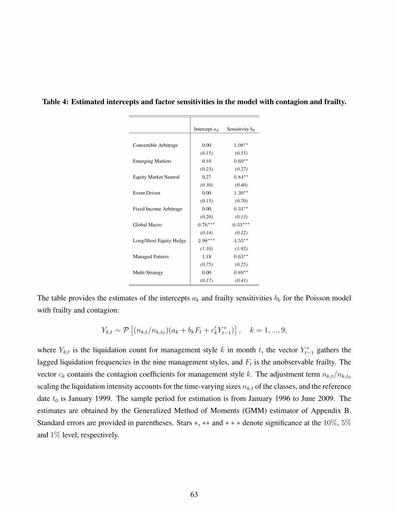
Table 4: Estimated intercepts and factor sensitivities in the model with contagion and frailty.

Intercept ak Sensitivity bk

Convertible Arbitrage 0.00 1.08∗∗

(0.15) (0.55)

Emerging Markets 0.10 0.69∗∗

(0.23) (0.27)

Equity Market Neutral 0.27 0.84∗∗

(0.30) (0.40)

Event Driven 0.00 1.39∗∗

(0.15) (0.70)

Fixed Income Arbitrage 0.00 0.31∗∗

(0.20) (0.13)

Global Macro 0.76∗∗∗ 0.33∗∗∗

(0.14) (0.12)

Long/Short Equity Hedge 2.98∗∗∗ 4.55∗∗

(1.10) (1.92)

Managed Futures 1.18 0.63∗∗

(0.75) (0.25)

Multi-Strategy 0.00 0.89∗∗

(0.17) (0.41)

The table provides the estimates of the intercepts ak and frailty sensitivities bk for the Poisson model

with frailty and contagion:

Yk,t ∼ P[(nk,t/nk,t0)(ak + bkFt + c′kY

∗t−1)

], k = 1, ..., 9,

where Yk,t is the liquidation count for management style k in month t, the vector Y ∗t−1 gathers the

lagged liquidation frequencies in the nine management styles, and Ft is the unobservable frailty. The

vector ck contains the contagion coefficients for management style k. The adjustment term nk,t/nk,t0

scaling the liquidation intensity accounts for the time-varying sizes nk,t of the classes, and the reference

date t0 is January 1999. The sample period for estimation is from January 1996 to June 2009. The

estimates are obtained by the Generalized Method of Moments (GMM) estimator of Appendix B.

Standard errors are provided in parentheses. Stars ∗, ∗∗ and ∗ ∗ ∗ denote significance at the 10%, 5%

and 1% level, respectively.

63

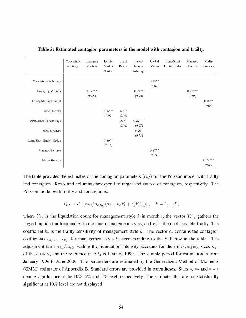
Table 5: Estimated contagion parameters in the model with contagion and frailty.

Convertible Emerging Equity Event Fixed Global Long/Short Managed Multi-

Arbitrage Markets Market Driven Income Macro Equity Hedge Futures Strategy

Neutral Arbitrage

Convertible Arbitrage 0.15∗∗

(0.07)

Emerging Markets 0.17∗∗∗ 0.21∗∗ 0.20∗∗∗

(0.06) (0.08) (0.05)

Equity Market Neutral 0.10∗∗

(0.05)

Event Driven 0.35∗∗∗ 0.10∗

(0.09) (0.06)

Fixed Income Arbitrage 0.09∗∗ 0.22∗∗∗

(0.04) (0.07)

Global Macro 0.20∗

(0.11)

Long/Short Equity Hedge 0.39∗∗

(0.16)

Managed Futures 0.27∗∗

(0.11)

Multi-Strategy 0.29∗∗∗

(0.06)

The table provides the estimates of the contagion parameters (ck,l) for the Poisson model with frailty

and contagion. Rows and columns correspond to target and source of contagion, respectively. The

Poisson model with frailty and contagion is:

Yk,t ∼ P[(nk,t/nk,t0)(ak + bkFt + c′kY

∗t−1)

], k = 1, ..., 9,

where Yk,t is the liquidation count for management style k in month t, the vector Y ∗t−1 gathers the

lagged liquidation frequencies in the nine management styles, and Ft is the unobservable frailty. The

coefficient bk is the frailty sensitivity of management style k. The vector ck contains the contagion

coefficients ck,1, ..., ck,9 for management style k, corresponding to the k-th row in the table. The

adjustment term nk,t/nk,t0 scaling the liquidation intensity accounts for the time-varying sizes nk,t

of the classes, and the reference date t0 is January 1999. The sample period for estimation is from

January 1996 to June 2009. The parameters are estimated by the Generalized Method of Moments

(GMM) estimator of Appendix B. Standard errors are provided in parentheses. Stars ∗, ∗∗ and ∗ ∗ ∗denote significance at the 10%, 5% and 1% level, respectively. The estimates that are not statistically

significant at 10% level are not displayed.

64

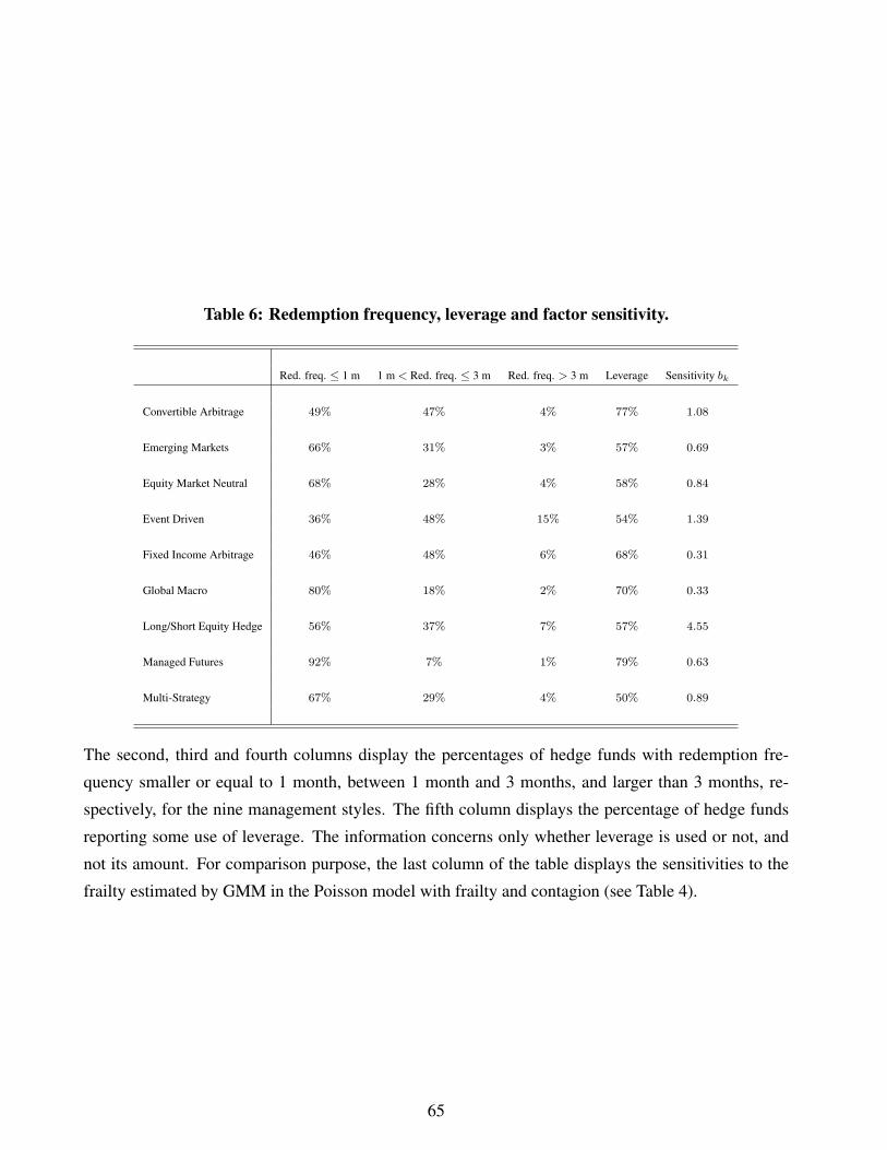
Table 6: Redemption frequency, leverage and factor sensitivity.

Red. freq. ≤ 1 m 1 m < Red. freq. ≤ 3 m Red. freq. > 3 m Leverage Sensitivity bk

Convertible Arbitrage 49% 47% 4% 77% 1.08

Emerging Markets 66% 31% 3% 57% 0.69

Equity Market Neutral 68% 28% 4% 58% 0.84

Event Driven 36% 48% 15% 54% 1.39

Fixed Income Arbitrage 46% 48% 6% 68% 0.31

Global Macro 80% 18% 2% 70% 0.33

Long/Short Equity Hedge 56% 37% 7% 57% 4.55

Managed Futures 92% 7% 1% 79% 0.63

Multi-Strategy 67% 29% 4% 50% 0.89

The second, third and fourth columns display the percentages of hedge funds with redemption fre-

quency smaller or equal to 1 month, between 1 month and 3 months, and larger than 3 months, re-

spectively, for the nine management styles. The fifth column displays the percentage of hedge funds

reporting some use of leverage. The information concerns only whether leverage is used or not, and

not its amount. For comparison purpose, the last column of the table displays the sensitivities to the

frailty estimated by GMM in the Poisson model with frailty and contagion (see Table 4).

65

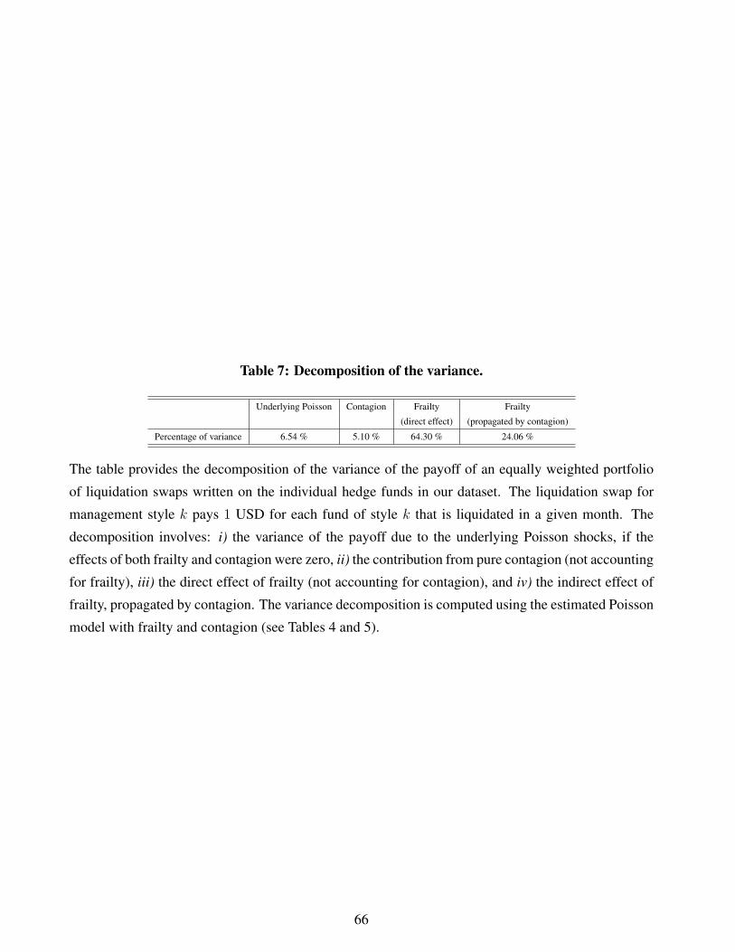
Table 7: Decomposition of the variance.

Underlying Poisson Contagion Frailty Frailty

(direct effect) (propagated by contagion)

Percentage of variance 6.54 % 5.10 % 64.30 % 24.06 %

The table provides the decomposition of the variance of the payoff of an equally weighted portfolio

of liquidation swaps written on the individual hedge funds in our dataset. The liquidation swap for

management style k pays 1 USD for each fund of style k that is liquidated in a given month. The

decomposition involves: i) the variance of the payoff due to the underlying Poisson shocks, if the

effects of both frailty and contagion were zero, ii) the contribution from pure contagion (not accounting

for frailty), iii) the direct effect of frailty (not accounting for contagion), and iv) the indirect effect of

frailty, propagated by contagion. The variance decomposition is computed using the estimated Poisson

model with frailty and contagion (see Tables 4 and 5).

66

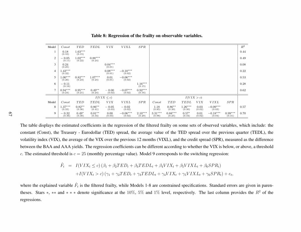
Table 8: Regression of the frailty on observable variables.

Model Const TED TEDL V IX V IXL SPR R2

1 0.18(0.10)

1.63∗∗∗(0.15)

0.44

2 − 0.05(0.11)

1.02∗∗∗(0.22)

0.88∗∗∗(0.24)

0.49

3 0.24(0.25)

0.04∗∗∗(0.01)

0.08

4 1.43∗∗∗(0.32)

0.08∗∗∗(0.01)

−0.10∗∗∗(0.02)

0.22

5 1.00∗∗∗(0.26)

0.82∗∗∗(0.23)

1.07∗∗∗(0.24)

0.01(0.01)

−0.06∗∗∗(0.02)

0.53

6 − 0.11(0.16)

1.16∗∗∗(0.15)

0.28

7 0.94∗∗∗(0.24)

0.95∗∗∗(0.21)

0.49∗∗(0.24)

− 0.00(0.02)

−0.07∗∗∗(0.02)

0.92∗∗∗(0.16)

0.62

I(V IX ≤ c) I(V IX > c)

Model Const TED TEDL V IX V IXL SPR Const TED TEDL V IX V IXL SPR

8 1.37∗∗∗(0.33)

0.82∗∗(0.36)

0.86∗∗(0.41)

− 0.05(0.03)

− 0.02(0.02)

1.18(0.85)

0.86∗∗(0.30)

1.26∗∗∗(0.30)

0.03(0.02)

−0.09∗∗∗(0.03)

0.57

9 − 0.32(0.36)

0.49∗(0.30)

0.81∗∗(0.34)

0.00(0.03)

−0.06∗∗∗(0.02)

2.10∗∗∗(0.29)

3.31∗∗∗(0.98)

0.88∗∗∗(0.25)

0.57∗(0.34)

0.01(0.02)

−0.18∗∗∗(0.04)

0.99∗∗∗(0.31)

0.70

The table displays the estimated coefficients in the regression of the filtered frailty on some sets of observed variables, which include: the

constant (Const), the Treasury - Eurodollar (TED) spread, the average value of the TED spread over the previous quarter (TEDL), the

volatility index (VIX), the average of the VIX over the previous 12 months (VIXL), and the credit spread (SPR), measured as the difference

between the BAA and AAA yields. The regression coefficients can be different according to whether the VIX is below, or above, a threshold

c. The estimated threshold is c = 25 (monthly percentage value). Model 9 corresponds to the switching regression:

Ft = I(V IXt ≤ c) (β1 + β2TEDt + β3TEDLt + β4V IXt + β5V IXLt + β6SPRt)

+I(V IXt > c) (γ1 + γ2TEDt + γ3TEDLt + γ4V IXt + γ5V IXLt + γ6SPRt) + et,

where the explained variable Ft is the filtered frailty, while Models 1-8 are constrained specifications. Standard errors are given in paren-

theses. Stars ∗, ∗∗ and ∗ ∗ ∗ denote significance at the 10%, 5% and 1% level, respectively. The last column provides the R2 of the

regressions.

67

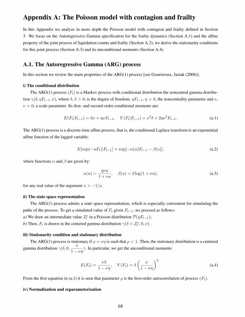
Appendix A: The Poisson model with contagion and frailty

In this Appendix we analyze in more depth the Poisson model with contagion and frailty defined in Section

3. We focus on the Autoregressive Gamma specification for the frailty dynamics (Section A.1) and the affine

property of the joint process of liquidation counts and frailty (Section A.2), we derive the stationarity conditions

for this joint process (Section A.3) and its unconditional moments (Section A.4).

A.1. The Autoregressive Gamma (ARG) process

In this section we review the main properties of the ARG(1) process [see Gourieroux, Jasiak (2006)].

i) The conditional distributionThe ARG(1) process (Ft) is a Markov process with conditional distribution the noncentral gamma distribu-

tion γ(δ, ηFt−1, ν), where δ, δ > 0, is the degree of freedom, ηFt−1, η > 0, the noncentrality parameter and ν,

ν > 0, a scale parameter. Its first- and second-order conditional moments are:

E(Ft|Ft−1) = δν + ηνFt−1, V (Ft|Ft−1) = ν2δ + 2ην2Ft−1. (a.1)

The ARG(1) process is a discrete-time affine process, that is, the conditional Laplace transform is an exponential

affine function of the lagged variable:

E[exp(−uFt)|Ft−1] = exp[−α(u)Ft−1 − β(u)], (a.2)

where functions α and β are given by:

α(u) =ηνu

1 + νu, β(u) = δ log(1 + νu), (a.3)

for any real value of the argument u > −1/ν.

ii) The state space representationThe ARG(1) process admits a state space representation, which is especially convenient for simulating the

paths of the process. To get a simulated value of Ft given Ft−1, we proceed as follows:

a) We draw an intermediate value Zst in a Poisson distribution P(ηFt−1);

b) Then, Ft is drawn in the centered gamma distribution γ(δ + Zst , 0, ν).

iii) Stationarity condition and stationary distributionThe ARG(1) process is stationary if ρ = νη is such that ρ < 1. Then, the stationary distribution is a centered

gamma distribution γ(δ, 0,ν

1− νη). In particular, we get the unconditional moments:

E(Ft) =νδ

1− νη, V (Ft) = δ

(ν

1− νη

)2

. (a.4)

From the first equation in (a.1) it is seen that parameter ρ is the first-order autocorrelation of process (Ft).

iv) Normalization and reparameterization

68

When theARG(1) process is used as a latent frailty, the scale of the process can be absorbed in the sensitivity

parameters bk of the intensity function in (3.1). Then, the process (Ft) can be normalized to have stationary

expectation E(Ft) = 1. Thus, from the first equation in (a.4), the parameters are such that νδ = 1−νη = 1−ρ.

It follows that the model can be parameterized in terms of δ and ρ, while the remaining parameters are given by:

ν =1− ρδ

, η =ρδ

1− ρ. (a.5)

The stationary distribution is γ(δ, 0, 1/δ), with Laplace transform E[exp(−uFt)] = (1 + u/δ)−δ, for u > −δ.

Moreover, the stationary variance is V (Ft) = 1/δ.

A.2 The affine property

In this section we show that the joint process of liquidation counts and frailty defined in System (4.2) is affine.

For completeness, we give the definition of the process in the next Assumption A.1.

Assumption A.1: The joint distribution of the liquidation counts Yt and frailty Ft given the past values Yt−1 =

(Yt−1, Yt−2, ...) and Ft−1 = (Ft−1, Ft−2, ...) is such that:

Yk,t|Yt−1, Ft ∼ P[(nk,t/nk,t0)

(ak + bkFt + c′kY

∗t−1

)], independent across k = 1, ...,K,

Ft|Yt−1, Ft−1 ∼ γ (δ, ηFt−1, ν) ,

where parameters η and ν are given in (a.5).

The liquidation counts of different management styles are conditionally independent given the past values of the

liquidation counts and the current and past values of the frailty. Moreover, the conditional distribution of the

frailty Ft is independent on the past liquidations counts. This condition corresponds to the exogeneity property

of the frailty process, which follows a ARG(1) process.

Let us now show that the joint process (Yt, Ft) is affine. By the moment generating function of the Poisson

distribution, we deduce that the conditional Laplace transform of the current liquidation counts vector Yt given

Ft and Yt−1 is:

ψt(u) = E[exp(−u′Yt)|Ft, Yt−1

]=∏k

E[exp(−ukYk,t)|Ft, Yt−1]

=∏k

exp {−γk,tλk,t[1− exp(−uk)]}

= exp

{−∑k

[1− exp(−uk)]γk,tak −∑k

[1− exp(−uk)]γk,tbkFt −∑k

[1− exp(−uk)]γk,tc′kY ∗t−1

},

(a.6)

where u is a vector with nonnegative components uk, and we use the notation λk,t = (nk,t/nk,t0)(ak + bkFt +

c′kY∗t−1) for the conditional intensity and γk,t = nk,t/nk,t0 for the size adjustment in management style k.

Moreover, by the exogenous ARG(1) dynamics of the frailty process, we have:

E[exp(−vFt)|Yt−1, Ft−1] = exp[−α(v)Ft−1 − β(v)], (a.7)

69

where functions α and β are given in (a.3). Then, from (a.6)-(a.7) and the Law of iterated expectation, we get

the conditional Laplace transform of the joint process (Y ′t , Ft)′ given its past:

ψt(u, v) = E[exp(−u′Yt − vFt)|Ft−1, Yt−1]

= E{E[exp(−u′Yt)|Ft, Yt−1

]exp(−vFt)|Ft−1, Yt−1

}= exp

{−∑k

γk,tak[1− exp(−uk)]−∑k

[1− exp(−uk)]γk,tc′kY ∗t−1

−α

∑k,

γk,tbk[1− exp(−uk)] + v

Ft−1 − β

(∑k

γk,tbk[1− exp(−uk)] + v

) .(a.8)

This joint conditional Laplace transform is exponential affine in lagged values Yt−1 and Ft−1, that is, it is of the

form:

ψt(u, v) = exp{−α1,t(u, v)′Yt−1 − α2,t(u, v)Ft−1 − βt(u, v)}, say, (a.9)

where the sensitivity coefficients α1,t, α2,t and βt depend on the class sizes and are time dependent in general.

Thus, process (Y ′t , Ft)′ is a time-heterogeneous affine Markov process. The closed form exponential affine

expression of the conditional Laplace transform of process (Y ′t , Ft)′ simplifies the computation of the predictive

distributions at any prediction horizon required in the stress-testing analysis, and the filtering of the latent factor

(see the online supplementary material). The closed form expression of the conditional Laplace transform

also provides informative moment restrictions, which are the basis of estimation with the Generalized Method

of Moments (see Appendix B). While we have kept the frailty process one-dimensional with ARG dynamics

for simplicity, the affine property of the joint process (Y ′t , Ft)′ remains valid as long as the frailty admits a

(multidimensional) affine dynamics.

A.3 Stationarity

In some applications such as stress testing (see Section 6), it is appropriate to consider a given portfolio structure

with respect to the management style, which is held fixed through time in the analysis. For this purpose, we

consider the next Assumption A.2 in the rest of this Appendix.

Assumption A.2: The size adjustments are constant and equal to 1: γk,t = 1, for any k, t.

Thus, the sizes of the categories are fixed through time, and are assumed homogeneous across management

styles for expository purpose.

Let us now derive the stationarity conditions for the joint process Zt = (Y ′t , Ft)′ under Assumptions A.1

and A.2. From equation (a.8), the conditional Laplace transform of the Markov process Zt is given by:

E[exp

(−w′Zt

)|Zt−1

]= exp

(−A(w)′Zt−1 −B(w)

),

where w = (u′, v)′ ∈ RK × R, functions A(w) and B(w) are given by:

A(w) =

[K∑k=1

c′k(1− e−uk), α

(v +

K∑k=1

(1− e−uk)bk

)]′,

70

and:

B(w) =K∑k=1

(1− e−uk)ak + β

(v +

K∑k=1

(1− e−uk)bk

),

and functions α and β are given in (a.3). Thus, process (Zt) is a time-homogeneous affine process. From

Proposition 2 in Darolles, Gourieroux, Jasiak (2006), process (Zt) is strictly stationary if:

limτ→∞

[∂A(0)∂w′

]τ= 0. (a.10)

Now, by using that∂A(0)∂uk

= [c′k, bkdα(0)/du]′ = [ck, ρbk]′, for k = 1, ...,K, and∂A(0)∂v

= [0′, dα(0)/du]′ =

[0′, ρ]′, we get:∂A(0)∂w′

=

(C 0

ρb′ ρ

).

Thus, condition (a.10) is satisfied if, and only if, the first-order autocorrelation of the frailty is such that ρ < 1

and the eigenvalues of the contagion matrix C have modulus smaller than 1.

A.4 Unconditional moments

In this section we derive the first- and second-order unconditional moments of the liquidation count process Ytunder the stationarity conditions derived in the previous section.

i) Moments of order 1From the conditional Poisson distribution of the counts, we have:

Et−1(Yt) = Et−1[Et−1(Yt|Ft)] = Et−1(a+ bFt + CYt−1) = a+ bEt−1(Ft) + CYt−1,

where Et−1 denotes expectation conditional on the past histories of liquidation counts Yt−1 and factor Ft−1.

By taking the expectation of both sides of the equation, and using the stationarity of process (Yt) and the

normalization E(Ft) = 1, we get:

E(Yt) = a+ b+ CE(Yt) ⇔ E(Yt) = (Id− C)−1(a+ b). (a.11)

ii) Moments of order 2Let us first consider the covariance between the liquidation counts and the frailty. We have:

Et−1(FtYt) = Et−1[Et−1(FtYt|Ft)] = Et−1[Ft(a+ bFt + CYt−1)]

= aEt−1(Ft) + bEt−1(F 2t ) + CEt−1(Ft)Yt−1

= aEt−1(Ft) + bEt−1(F 2t ) + C(1− ρ+ ρFt−1)Yt−1,

from equations (a.1) and (a.5). By taking the expectation of both sides of the equation, we get:

E(FtYt) = a+ b(1 + σ2) + (1− ρ)C(Id− C)−1(a+ b) + ρCE(FtYt),

71

where σ2 = V (Ft) = 1/δ denotes the variance of the frailty [see Section A.1 iv)]. We deduce that:

E(FtYt) = (Id− ρC)−1{bσ2 + [Id+ (1− ρ)C(Id− C)−1](a+ b)},

= (Id− ρC)−1bσ2 + (Id− C)−1(a+ b).

Thus:

Cov(Yt, Ft) = σ2(Id− ρC)−1b. (a.12)

Let us now consider the variance-covariance matrix of the liquidation counts vector Yt. We have:

Et−1(YtY ′t ) = Et−1(Et−1[YtY ′t |Ft]) = Et−1[Vt−1(Yt|Ft) + Et−1(Yt|Ft)Et−1(Yt|Ft)′]

= Et−1[diag(a+ bFt + CYt−1)] + Et−1[(a+ bFt + CYt−1)(a+ bFt + CYt−1)′]

= diag[a+ bEt−1(Ft) + CYt−1] + bb′Vt−1(Ft)

+[Et−1(a+ bFt + CYt−1)][Et−1(a+ bFt + CYt−1)]′

= diag[a+ bEt−1(Ft) + CYt−1] + bb′Vt−1(Ft)

+[a+ b(1− ρ+ ρFt−1) + CYt−1][a+ b(1− ρ+ ρFt−1) + CYt−1]′.

By taking the expectation of both sides, we deduce:

E(YtY ′t ) = diag[a+ b+ C(Id− C)−1(a+ b)] + bb′E[Vt−1(Ft)] + V [bρFt−1 + CYt−1]

+E[a+ b(1− ρ+ ρFt−1) + CYt−1]E[a+ b(1− ρ+ ρFt−1) + CYt−1]′

= diag[(Id− C)−1(a+ b)] + σ2(1− ρ2)bb′ + V [bρFt−1 + CYt−1] + E(Yt)E(Y ′t ),

where we use that E[Vt−1(Ft)] = σ2(1 − ρ2). Therefore, the variance-covariance matrix of Yt satisfies the

recursive equation:

V (Yt) = CV (Yt)C ′ + diag[(Id− C)−1(a+ b)] + σ2bb′

+ρbCov(Ft, Yt)C ′ + ρCCov(Yt, Ft)b′. (a.13)

Equation (4.3) is obtained by substituting the expression (a.12) of Cov(Yt, Ft).

iii) Autocovariance at order 1We have:

Cov(Yt, Yt−1) = Cov[Et−1(Yt), Yt−1] = Cov[Et−1(a+ bFt + CYt−1), Yt−1]

= Cov[a+ b(1− ρ+ ρFt−1) + CYt−1, Yt−1].

Therefore:

Cov(Yt, Yt−1) = Cov(bρFt−1 + CYt−1, Yt−1) = bρCov(Ft−1, Yt−1) + CV (Yt)

= CV (Yt) + σ2ρbb′(Id− ρC ′)−1. (a.14)

72

Appendix B: GMM estimation of the Poisson model with frailtyand contagion

In this Appendix we develop an estimation approach for the parameters of the Poisson model with contagion and

frailty that is based on the Generalized Method of Moments [GMM, Hansen (1982), Hansen, Singleton (1982)].

We start by considering moment restrictions that involve the liquidation intensity parameters and the parameters

in the stationary distribution of the frailty only (Section B.1). We then present moment restrictions that involve

the autoregressive parameter of the frailty as well (Section B.2). Finally, we discuss the implementation of the

associated GMM estimators (Section B.3).

B.1 Static moment restrictions

The moment restrictions are based on the special form of the conditional Laplace transform in equation (a.6).

For management style k we have:

E[exp (−ukYk,t) |Ft, Yt−1] = exp{−γk,t

(ak + bkFt + c′kY

∗t−1

)(1− e−uk)

}, (b.1)

for any argument uk ∈ [0,∞). These conditional moments are appropriate for analyzing risk parameters.

Indeed, the left hand side of the above equation is simply the expected utility function for an investor with a

portfolio totally invested in the liquidation events of style k, and an absolute risk aversion equal to uk. By

considering the associated set of moment restrictions, we consider all types of investment, for all values of risk

aversion. Therefore, the associated moment method will calibrate the unknown parameters on the whole set of

expected utilities.

The equations in (b.1) can be rewritten as:

E[exp

{−ukYk,t + γk,t

(ak + c′kY

∗t−1

)(1− e−uk)

}|Ft, Yt−1

]= exp

{−γk,tbk(1− e−uk)Ft

}, (b.2)

for uk ∈ [0,∞). Thus, we obtain nonlinear transforms of the observable liquidation count variables, whose

conditional expectation depends on the frailty only. As equation (b.2) holds for all real positive arguments uk,

we can consider a time-dependent argument uk. The time dependence is selected such that the RHS of equation

(b.2), and thus the LHS as well, is stationary. More precisely, let uk,t be such that 1− e−uk,t = v/γk,t, for given

v ∈ Vk, i.e. uk,t = − log (1− v/γk,t). In order to obtain a well-defined uk,t in [0,∞), the real interval Vk has

to be a subset of [0, inftγk,t). Then, equation (b.2) becomes:

E[exp

{log(1− v/γk,t)Yk,t + v

(ak + c′kY

∗t−1

)}|Ft, Yt−1

]= exp (−vbkFt) , ∀v ∈ Vk. (b.3)

These moment restrictions are conditional on factor path Ft and cannot be used directly for estimation since the

factor is unobservable. Therefore, we integrate out the latent factor by taking expectation on both sides of the

equation w.r.t. the gamma stationary distribution γ(δ, 0, 1/δ) of factor process Ft [see Appendix A.1 iv)]. We

get a continuum of unconditional moment restrictions:

E[exp

{log(1− v/γk,t)Yk,t + v

(ak + c′kY

∗t−1

)}]=

1

(1 + vbk/δ)δ, ∀v ∈ Vk. (b.4)

73

These static moment restrictions involve the intensity parameters ak, bk, ck for any type k, as well as parameter

δ characterizing the stationary distribution of the frailty, but do not allow to identify the frailty persistence

parameter ρ.

B.2 Dynamic moment restrictions

In order to derive moment restrictions that allow for estimation of parameter ρ, let us consider equation (b.3)

and multiply both sides by exp(−ul,t−1Yl,t−1), where ul,t−1 = − log(1 − v/γl,t−1), for some type l and any

v ∈ Vl. We have:

E[exp

{−uk,tYk,t − ul,t−1Yl,t−1 + v

(ak + c′kY

∗t−1

)}|Ft, Yt−1

]= exp (−vbkFt − ul,t−1Yl,t−1) ,

for all v ∈ Vk, v ∈ Vl, where uk,t = log(1 − v/γk,t). By taking the conditional expectation given Ft and the

liquidation counts history Yt−2 up to month t− 2 on both sides of the equation, we get:

E[exp

{−uk,tYk,t − ul,t−1Yl,t−1 + v

(ak + c′kY

∗t−1

)}|Ft, Yt−2

]= exp (−vbkFt)E

[exp (−ul,t−1Yl,t−1) |Ft, Yt−2

]= exp

{−vbkFt − (al + blFt−1 + c′lY

∗t−2)v

}.

By rearranging terms, and computing the unconditional expectation of both sides, we get:

E[exp

{−uk,tYk,t − ul,t−1Yl,t−1 + v

(ak + c′kY

∗t−1

)+ v

(al + c′lY

∗t−2

)}]= E [exp (−vbkFt − vblFt−1)] ,

for all v ∈ Vk, v ∈ Vl. The expectation in the right-hand side involves the joint distribution of the frailty values

Ft and Ft−1 on two consecutive months, and hence depends on the frailty autocorrelation parameter ρ. In fact,

by the exponential affine property of the ARG process (see Appendix A.1) we have:

E [exp (−vbkFt − vblFt−1)]

= E [E[exp (−vbkFt) |Ft−1] exp (−vblFt−1)] = exp (−β(vbk))E [exp (−[α(vbk) + vbl]Ft−1)]

=1

[1 + (1− ρ)vbk/δ]δ1

[1 + [α(bvk) + vbl]/δ]δ

=1

[1 + (vbk + vbl)/δ + (1− ρ)vvbkbl/δ2]δ,

where we use β(u) = δ log(1 + (1− ρ)u/δ) and α(u) =ρu

1 + (1− ρ)u/δfrom equations (a.3) and (a.5). Thus,

we get the continuum of unconditional dynamic moment restrictions:

E[exp

{log(1− v/γk,t)Yk,t + log(1− v/γl,t−1)Yl,t−1 + v

(ak + c′kY

∗t−1

)+ v

(al + c′lY

∗t−2

)}]=

1

[1 + (vbk + vbl)/δ + (1− ρ)vvbkbl/δ2]δ, ∀v ∈ Vk, v ∈ Vl. (b.5)

These dynamic moment restrictions, written for all pairs of management styles (k, l), involve all model param-

eters. For v = 0, these moment restrictions reduce to the static moment restrictions (b.4).

74

B.3 GMM estimators

The moment restrictions in Sections B.1 and B.2 can be used in different ways to define GMM estimators. We

consider below three possible GMM approaches.

i) We can use the static moment restrictions (b.4) written for all types k to define a first-step GMM estimator

of parameters ak, bk, ck, for all management styles k, and parameter δ. Then, a second-step GMM estimator

of parameter ρ can be defined by using some subset of the dynamic moment restrictions (b.5) and replacing

parameters ak, bk, ck and δ with their first-step GMM estimates.

ii) Alternatively, the dynamic moment restrictions (b.5) can be used to estimate jointly all model parameters

(θ′, ϕ′)′, where θ = (ak, bk, c′k, k = 1, ...,K)′ and ϕ = (δ, ρ)′, in one step. More precisely, consider the dynamic

moment restrictions (b.5) written for all management styles k, with l = k, and for a given grid of values v, v. 14

They define a set of unconditional moment restrictions E [hk,t(ak, bk, ck, ϕ)] = 0, for k = 1, ...,K, say, where

the hk,t are the moment functions. Then, the GMM estimator (θ′, ϕ′)′ minimizes the criterion:

QT (θ, ϕ) =K∑k=1

‖hk,T (ak, bk, ck, ϕ)‖2, (b.6)

where hk,T (ak, bk, ck, ϕ) =1T

T∑t=1

hk,t(ak, bk, ck, ϕ) is the sample average of the orthogonality function. By

including only the moment restrictions with k = l, and using a weighting matrix that is diagonal across man-

agement styles, we simplify considerably the optimization problem. 15 In fact, for given value of the bivariate

frailty parameter ϕ = (δ, ρ)′, the GMM criterion (b.6) is additive w.r.t. the parameters of the styles. Therefore,

the minimization can be performed by concentrating w.r.t. parameter θ. Namely, for given ϕ, the criteria for the

different styles k are separately minimized w.r.t. parameters ak, bk, ck by a Newton-Raphson algorithm. Then,

the concentrated criterion is minimized by a bi-dimensional grid search over parameters (δ, ρ).

iii) We can also consider the GMM estimators that exploit the full set of dynamic moment restrictions

(b.5) written for all pairs of management styles (k, l). Such GMM estimators are expected to be more efficient

than the GMM estimator minimizing criterion (b.6). However, such GMM estimators are computationally less

convenient, because they involve an optimization over a large-dimensional parameter space that can not be dealt

with by concentration easily.

In this paper we apply method ii), which provides a trade-off between tractability and efficiency.

14It might also be possible to apply an efficient GMM taking into account the continuum of moment restrictions (b.5)[see e.g. Carrasco et al (2007)].

15For expository purpose the weighting matrix is set equal to the identity matrix for each type.

75