1

Surge Modeling Tips and Procedures

Dr. Don J. Wood & Dr. Srinivasa Lingireddy

This Document contains a collection of answers to often asked questions, tips and

advice for surge modeling. As always please contact Dr. Wood, Dr. Lingireddy or one

of our other support staff if you have questions.

Length Tolerance

Using Pump Files

Sizing Compressor and Bladder Surge Tanks Using Surge

Handling Cavitation at SDO Devices

Surge Model Results – Excessive Pressure Spiking

Using Reduced Wave Speeds in Pump Stations

Check Valve Modeling and Responses

Trapped High Pressure Liquid

Fixed vs. Pressure Sensitive Demands

Dynamic vs. Static Friction

Comparing she MOC and the WCM

Convergence Issues Due to Pump Curve Shape

How to Create a Custom Pump File (Suter diagram)

Using Control Valves for Surge Protection

2

Length Tolerance

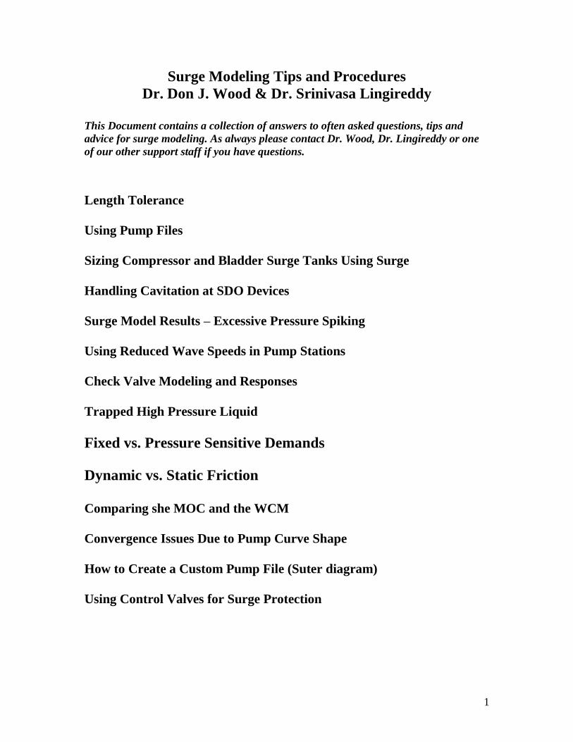
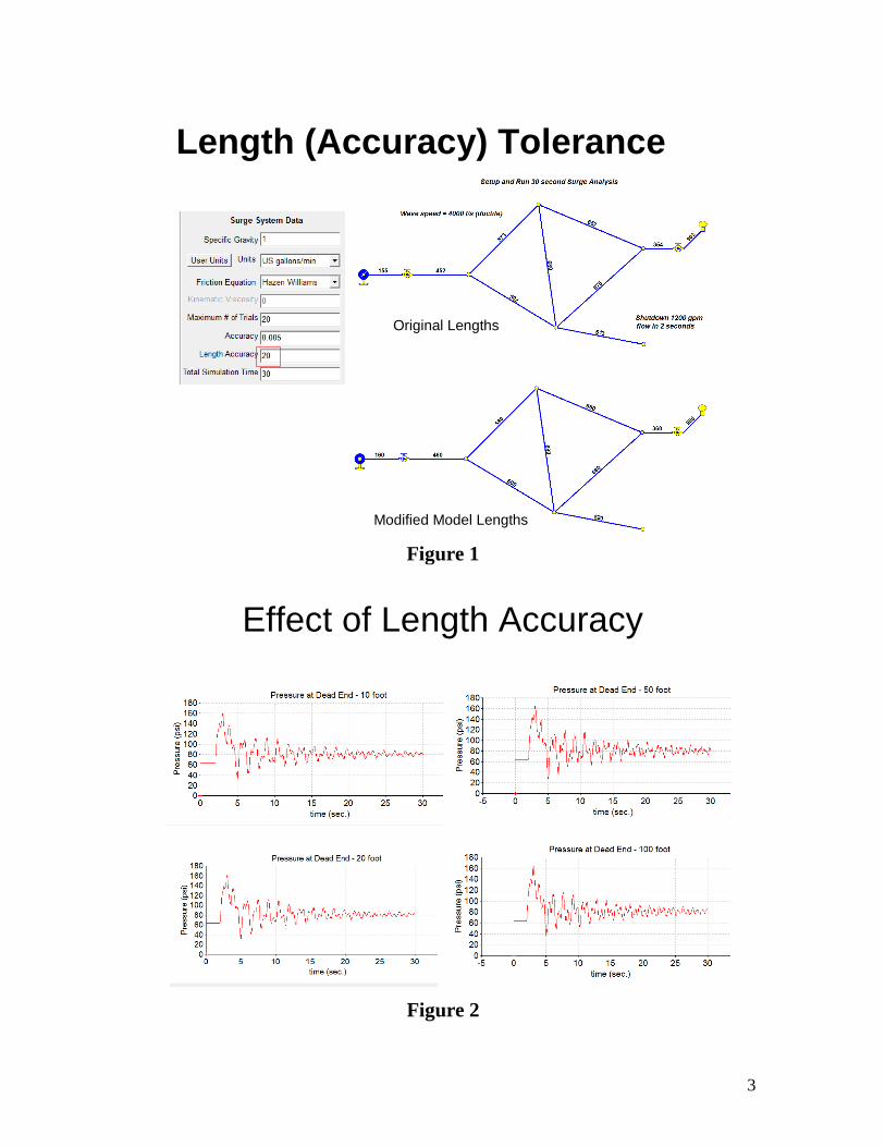
This input defaults to 10 ft (3 m) and represents the maximum difference between the

actual pipe lengths and the ones chosen for the model. Note the calculation time

increment and required computational time are affected by this selection and decreasing

the length accuracy by a factor of two will double the required computational time.

Pipe lengths (or wave speeds) in the model must be adjusted so each pipe will be a length

– wave speed combination such that the pressure wave will traverse the pipe in a time

which is an exact integer multiple of the computational time increment. Lengths will be

rounded to the nearest multiple of the Length Accuracy (not including 0), therefore the

maximum difference between adjusted pipe lengths in the model and actual system is

usually Length Accuracy/2. For example if we use Length Accuracy = 20 the lengths will

be rounded to the nearest multiple of 20 and the largest difference between the model

adjusted lengths and actual length is 10 feet (say 380 feet for a 389 foot pipe). This does

not hold for pipes which are shorter than the Length Accuracy. The adjusted pipe length

will be equal to the Length Accuracy so that the maximum difference is <= Length

Accuracy. For example if a pipe is 0.5 feet long and the Length Accuracy is 10, then the

adjusted pipe length will be 10 ft or 9.5 feet of difference.

It is important therefore for the Length Accuracy to be similar in value to the length of

the smaller pipes in the model.

While the shortest pipe in the model often does set the time step this is not always the

case. We determine the largest time step we can use and meet the length tolerance for all

pipes in the model. The figure below illustrates the process of adjusting lengths.

3

Length (Accuracy) Tolerance

Original Lengths

Modified Model Lengths

Figure 1

Effect of Length Accuracy

Figure 2

4

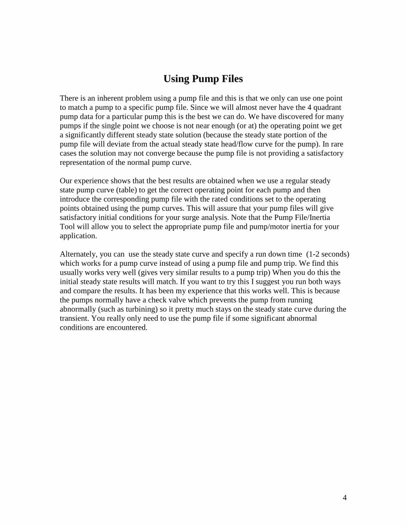
Using Pump Files

There is an inherent problem using a pump file and this is that we only can use one point

to match a pump to a specific pump file. Since we will almost never have the 4 quadrant

pump data for a particular pump this is the best we can do. We have discovered for many

pumps if the single point we choose is not near enough (or at) the operating point we get

a significantly different steady state solution (because the steady state portion of the

pump file will deviate from the actual steady state head/flow curve for the pump). In rare

cases the solution may not converge because the pump file is not providing a satisfactory

representation of the normal pump curve.

Our experience shows that the best results are obtained when we use a regular steady

state pump curve (table) to get the correct operating point for each pump and then

introduce the corresponding pump file with the rated conditions set to the operating

points obtained using the pump curves. This will assure that your pump files will give

satisfactory initial conditions for your surge analysis. Note that the Pump File/Inertia

Tool will allow you to select the appropriate pump file and pump/motor inertia for your

application.

Alternately, you can use the steady state curve and specify a run down time (1-2 seconds)

which works for a pump curve instead of using a pump file and pump trip. We find this

usually works very well (gives very similar results to a pump trip) When you do this the

initial steady state results will match. If you want to try this I suggest you run both ways

and compare the results. It has been my experience that this works well. This is because

the pumps normally have a check valve which prevents the pump from running

abnormally (such as turbining) so it pretty much stays on the steady state curve during the

transient. You really only need to use the pump file if some significant abnormal

conditions are encountered.

5

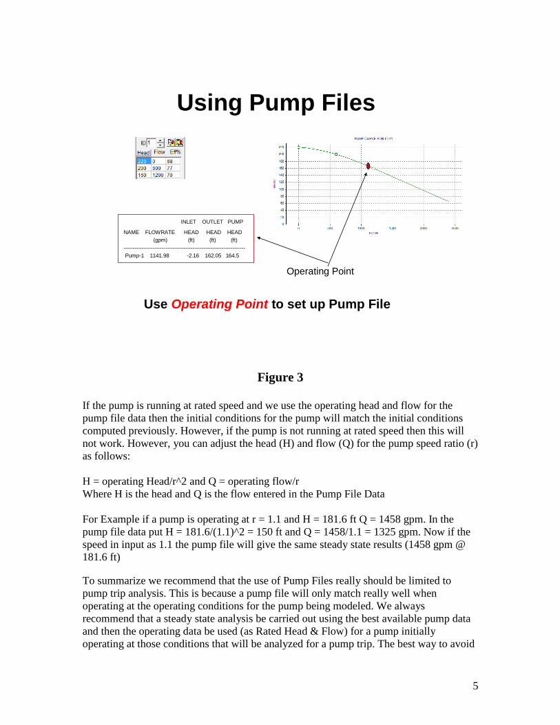
Using Pump Files

• INLET OUTLET PUMP

• NAME FLOWRATE HEAD HEAD HEAD

• (gpm) (ft) (ft) (ft)

• -------------------------------------------------------------------

• Pump-1 1141.98 -2.16 162.05 164.5

Operating Point

Use Operating Point to set up Pump File

Figure 3

If the pump is running at rated speed and we use the operating head and flow for the

pump file data then the initial conditions for the pump will match the initial conditions

computed previously. However, if the pump is not running at rated speed then this will

not work. However, you can adjust the head (H) and flow (Q) for the pump speed ratio (r)

as follows:

H = operating Head/r^2 and Q = operating flow/r

Where H is the head and Q is the flow entered in the Pump File Data

For Example if a pump is operating at r = 1.1 and H = 181.6 ft Q = 1458 gpm. In the

pump file data put H = 181.6/(1.1)^2 = 150 ft and Q = 1458/1.1 = 1325 gpm. Now if the

speed in input as 1.1 the pump file will give the same steady state results (1458 gpm @

181.6 ft)

To summarize we recommend that the use of Pump Files really should be limited to

pump trip analysis. This is because a pump file will only match really well when

operating at the operating conditions for the pump being modeled. We always

recommend that a steady state analysis be carried out using the best available pump data

and then the operating data be used (as Rated Head & Flow) for a pump initially

operating at those conditions that will be analyzed for a pump trip. The best way to avoid

6

problems associated with Pump Files is to Only use a Pump File for a Pump Trip

analysis.

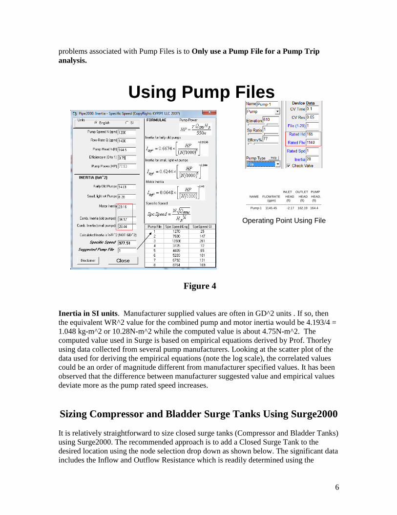
Using Pump Files

INLET OUTLET PUMP

NAME FLOWRATE HEAD HEAD HEAD.

(gpm) (ft) (ft) (ft)

------------------------------------------------------------------------Pump-1 1145.45 -2.17 162.19 164.4

Operating Point Using File

Figure 4

Inertia in SI units. Manufacturer supplied values are often in GD^2 units . If so, then

the equivalent WR^2 value for the combined pump and motor inertia would be 4.193/4 =

1.048 kg-m^2 or 10.28N-m^2 while the computed value is about 4.75N-m^2. The

computed value used in Surge is based on empirical equations derived by Prof. Thorley

using data collected from several pump manufacturers. Looking at the scatter plot of the

data used for deriving the empirical equations (note the log scale), the correlated values

could be an order of magnitude different from manufacturer specified values. It has been

observed that the difference between manufacturer suggested value and empirical values

deviate more as the pump rated speed increases.

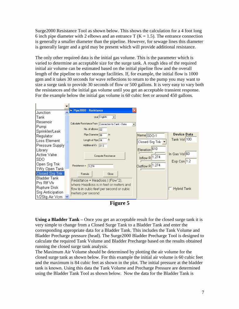
Sizing Compressor and Bladder Surge Tanks Using Surge2000

It is relatively straightforward to size closed surge tanks (Compressor and Bladder Tanks)

using Surge2000. The recommended approach is to add a Closed Surge Tank to the

desired location using the node selection drop down as shown below. The significant data

includes the Inflow and Outflow Resistance which is readily determined using the

7

Surge2000 Resistance Tool as shown below. This shows the calculation for a 4 foot long

6 inch pipe diameter with 2 elbows and an entrance T (K = 1.5). The entrance connection

is generally a smaller diameter than the pipeline. However, for sewage lines this diameter

is generally larger and a grid may be present which will provide additional resistance.

The only other required data is the initial gas volume. This is the parameter which is

varied to determine an acceptable size for the surge tank. A rough idea of the required

initial air volume can be estimated based on the initial pipeline flow and the overall

length of the pipeline to other storage facilities. If, for example, the initial flow is 1000

gpm and it takes 30 seconds for wave reflections to return to the pump you may want to

size a surge tank to provide 30 seconds of flow or 500 gallons. It is very easy to vary both

the resistances and the initial gas volume until you get an acceptable transient response.

For the example below the initial gas volume is 60 cubic feet or around 450 gallons.

Figure 5

Using a Bladder Tank – Once you get an acceptable result for the closed surge tank it is

very simple to change from a Closed Surge Tank to a Bladder Tank and enter the

corresponding appropriate data for a Bladder Tank. This includes the Tank Volume and

Bladder Precharge pressure (head). The Surge2000 Bladder Precharge Tool is designed to

calculate the required Tank Volume and Bladder Precharge based on the results obtained

running the closed surge tank analysis.

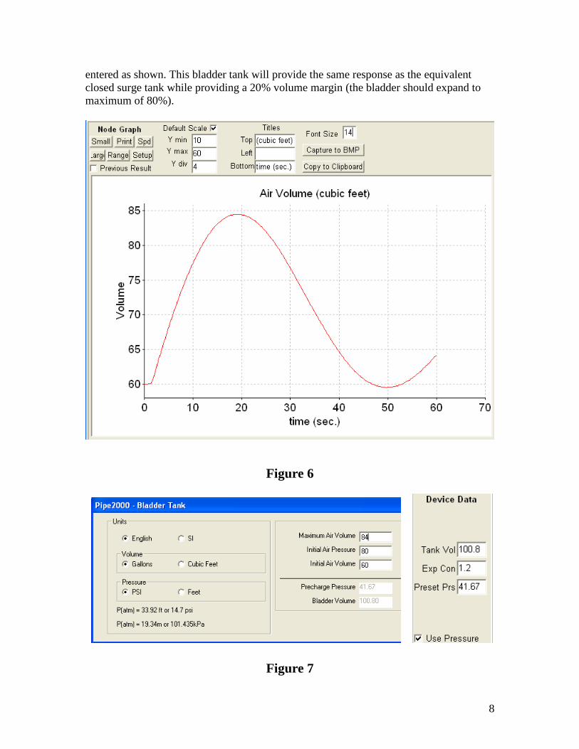
The Maximum Air Volume should be determined by plotting the air volume for the

closed surge tank as shown below. For this example the initial air volume is 60 cubic feet

and the maximum is 84 cubic feet as shown in the plot. The initial pressure at the bladder

tank is known. Using this data the Tank Volume and Precharge Pressure are determined

using the Bladder Tank Tool as shown below. Now the data for the Bladder Tank is

8

entered as shown. This bladder tank will provide the same response as the equivalent

closed surge tank while providing a 20% volume margin (the bladder should expand to

maximum of 80%).

Figure 6

Figure 7

9

Damping of Surges at zero flow

You may notice that the model predicts that transients damp out very slowly when

systems are shut down. The reason that the transient doesn't damp out more rapidly is due

to the way resistance is modeled. For both the Darcy Weisbach and the Hazen Williams

approach the resistance in a pipe is assumed to be a constant term which is determined

using the starting conditions, i.e. the resistance for a pipe section is the initial head drop

divided by the initial flow squared. We actually use this approach to calculate pipe

segment resistance for all situations. What this does is ignore the fact that pipe resistance

increases very much as the flow approaches zero. Therefore the models don't damp the

wave nearly as fast as they should when the final flow is zero as in a complete shutdown.

To illustrate this situation put in a valve with only a small initial loss (so it has little effect

in the steady state) Then close the valve to 99% after the system shutdown. This creates

a large resistance which quickly damps the wave. Without this the small initial pipe

resistances damp the waves very slowly.

In general this causes no significant problems in surge modeling. The magnitude of the

transients which are generated by an event are not really affected significantly by using a

constant pipe resistance - just the rate of damping. Note that this situation only shows up

(slow damping) for systems where the final flows are zero - if the final flow is non zero

then the constant pipe resistance works quite well to provide damping effects

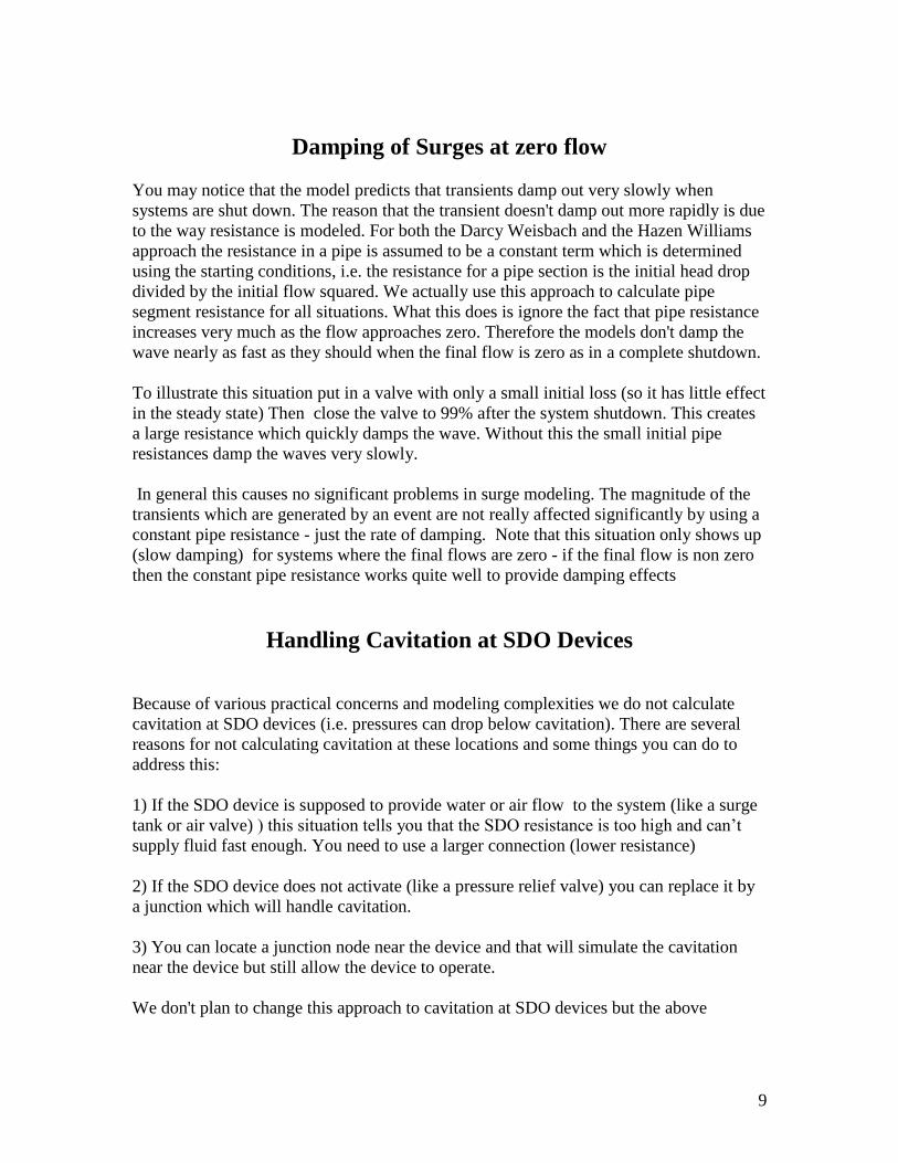
Handling Cavitation at SDO Devices

Because of various practical concerns and modeling complexities we do not calculate

cavitation at SDO devices (i.e. pressures can drop below cavitation). There are several

reasons for not calculating cavitation at these locations and some things you can do to

address this:

1) If the SDO device is supposed to provide water or air flow to the system (like a surge

tank or air valve) ) this situation tells you that the SDO resistance is too high and can’t

supply fluid fast enough. You need to use a larger connection (lower resistance)

2) If the SDO device does not activate (like a pressure relief valve) you can replace it by

a junction which will handle cavitation.

3) You can locate a junction node near the device and that will simulate the cavitation

near the device but still allow the device to operate.

We don't plan to change this approach to cavitation at SDO devices but the above

10

technique should handle situations when the user is concerned because pressures fall

below cavitation at SDO devices.

Handling Cavitation at SDO Devices

Cavitation indicates resistance is too high – device can’t perform

Figure 8

11

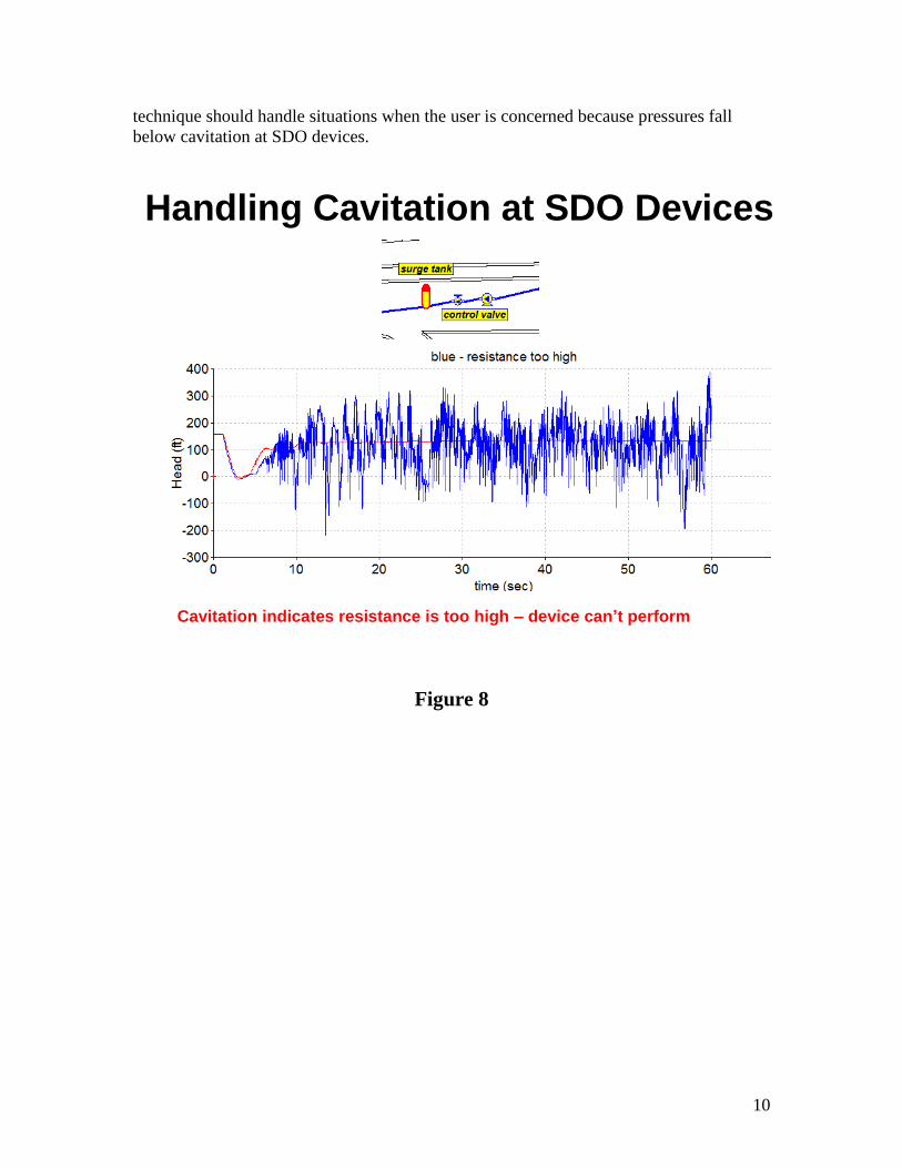
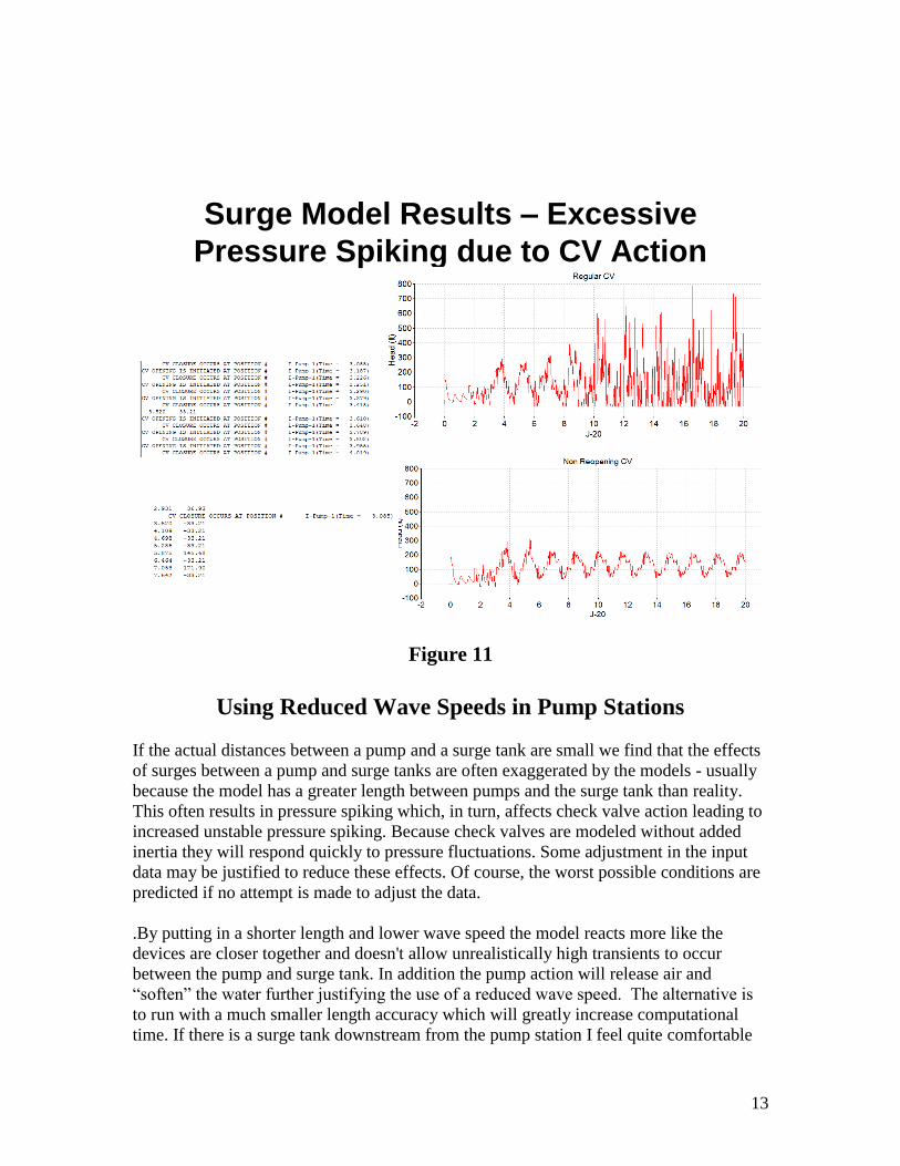
Surge Model Results – Excessive Pressure Spiking

Sometimes the results of a transient analysis show excessive spiking of the pressure as

shown

Figure 9

The solution may continue as pressure spikes and no final steady state result will be

reached. The spikes may even grow and reach very high values. This occurrence is

almost always due to:

1) Cavitation – spikes generated due to cavity collapse

2) Check Valve action – opening and closing of CV’s. A review of the tabulated

results report will indicate whether this action is occurring because check valve

action is noted in this report.

Either one or a combination of these situations can produce this type of result.

If this type of solution occurs due to check valve action at a pump which has been shut

down then the pump is operating in an abnormal fashion (flow reversals, etc.). Therefore,

it is essential that a pump file be used in the analysis and the pump trip option used for

the pump shutdown. In this manner the behavior of the pump can be calculated. Also the

effects of inertia and check valve properties can be evaluated.

12

When these results are obtained it is important to view the results more in a qualitative

than quantitative manner. The actual calculated magnitude of the spikes are very sensitive

to the system data and small changes can significantly affect the magnitude of the

pressure spikes. The important result is that the response is very volatile and unstable.

Because of the sensitivity of actual spike magnitudes to the timing of the events and data

it is not reasonable to compare solutions based on the highest calculated pressure spikes.

The solutions are just too sensitive. What can be concluded is that the transients can be

unstable and excessive pressure spikes are possible.

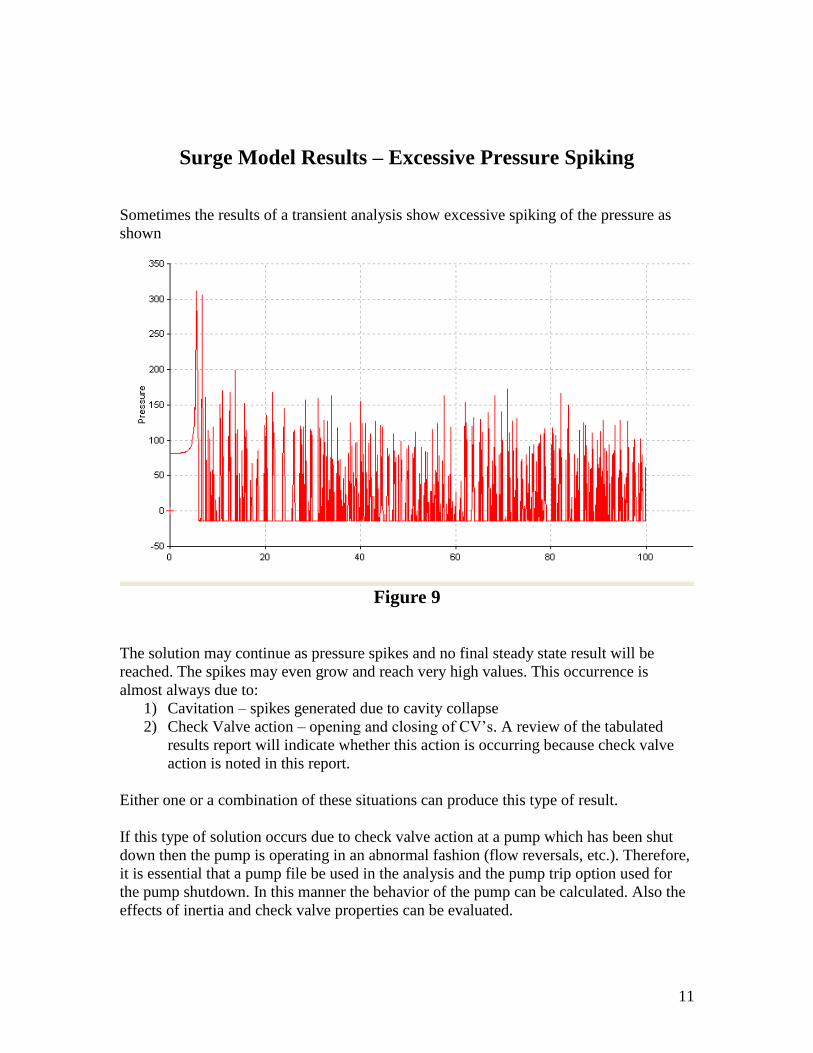
If you want to further evaluate the cause of an unstable result you can:

1) Set the default Cavitation Head to a very low value (such as -1000 ft. (m)). When

this is done and cavitation and the resulting unstable solution does not occur you

will know that cavity collapse is the cause of the pressure spiking..

2) Either remove check valves or set them to non reopening type so they will not

constantly open and close.

These actions should allow for the calculation of a stable response and will allow you to

evaluate the cause of the instability for your system.

Surge Model Results – Excessive

Pressure Spiking due to Cavitation

Figure 10

13

Surge Model Results – Excessive

Pressure Spiking due to CV Action

Figure 11

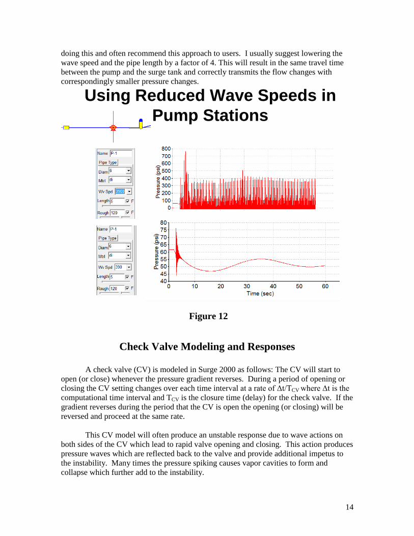
Using Reduced Wave Speeds in Pump Stations

If the actual distances between a pump and a surge tank are small we find that the effects

of surges between a pump and surge tanks are often exaggerated by the models - usually

because the model has a greater length between pumps and the surge tank than reality.

This often results in pressure spiking which, in turn, affects check valve action leading to

increased unstable pressure spiking. Because check valves are modeled without added

inertia they will respond quickly to pressure fluctuations. Some adjustment in the input

data may be justified to reduce these effects. Of course, the worst possible conditions are

predicted if no attempt is made to adjust the data.

.By putting in a shorter length and lower wave speed the model reacts more like the

devices are closer together and doesn't allow unrealistically high transients to occur

between the pump and surge tank. In addition the pump action will release air and

“soften” the water further justifying the use of a reduced wave speed. The alternative is

to run with a much smaller length accuracy which will greatly increase computational

time. If there is a surge tank downstream from the pump station I feel quite comfortable

14

doing this and often recommend this approach to users. I usually suggest lowering the

wave speed and the pipe length by a factor of 4. This will result in the same travel time

between the pump and the surge tank and correctly transmits the flow changes with

correspondingly smaller pressure changes.

Using Reduced Wave Speeds in

Pump Stations

Figure 12

Check Valve Modeling and Responses

A check valve (CV) is modeled in Surge 2000 as follows: The CV will start to

open (or close) whenever the pressure gradient reverses. During a period of opening or

closing the CV setting changes over each time interval at a rate of Δt/TCV where Δt is the

computational time interval and TCV is the closure time (delay) for the check valve. If the

gradient reverses during the period that the CV is open the opening (or closing) will be

reversed and proceed at the same rate.

This CV model will often produce an unstable response due to wave actions on

both sides of the CV which lead to rapid valve opening and closing. This action produces

pressure waves which are reflected back to the valve and provide additional impetus to

the instability. Many times the pressure spiking causes vapor cavities to form and

collapse which further add to the instability.

15

This action is all based on an accurate surge analysis for the check valve model

used in Surge2000. When you get this response you should realize that CV action can

produce unstable responses and large pressure surges. However, for a number of reasons

the model may over predict the instability. Some factors are:

1 Air released which dampens the action.

2 The model assumes air instantaneous response for the check valve (it will

start to open or change directions at the instant the pressure gradient

switches.)

3 If the suction line is modeled rapid pressure changes occur in the suction

line increasing the CV action.

4 Time delays for closing may allow significant velocity to develop just prior

to closure – causing pressure surges.

There are several ways to reduce or eliminate the instable CV responses obtained

by your model..

1 Use a non reopening CV. This device will close only one time and will

remain closed.

2 Eliminate the suction line by modeling the pump connected directly to the

supply reservoir.

3 Reduce the CV closing time (time delay).

.

In general I do not believe these actions causes any major problems in surge modeling

and can be employed. However, situations where check valve action leading to pressure

spiking and failures have been observed. A conservative design will model the piping

and devices within the pump station and address any predicted instabilities.

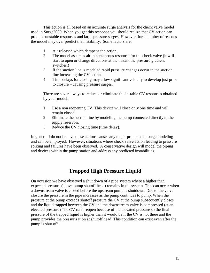
Trapped High Pressure Liquid

On occasion we have observed a shut down of a pipe system where a higher than

expected pressure (above pump shutoff head) remains in the system. This can occur when

a downstream valve is closed before the upstream pump is shutdown. Due to the valve

closure the pressure in the pipe increases as the pump continues to pump. When the

pressure at the pump exceeds shutoff pressure the CV at the pump subsequently closes

and the liquid trapped between the CV and the downstream valve is compressed (at an

elevated pressure) The CV can't reopen because of the elevated pressure so the final

pressure of the trapped liquid is higher than it would be if the CV is not there and the

pump provides the pressurization at shutoff head. This condition can exist even after the

pump is shut off.

16

Trapped High Pressure Liquid

1) Valve Closes

2) Pump runs – liquid compresses

3) Flow reverses

4) Pump CV closes trapping compressed liquid

Figure 13

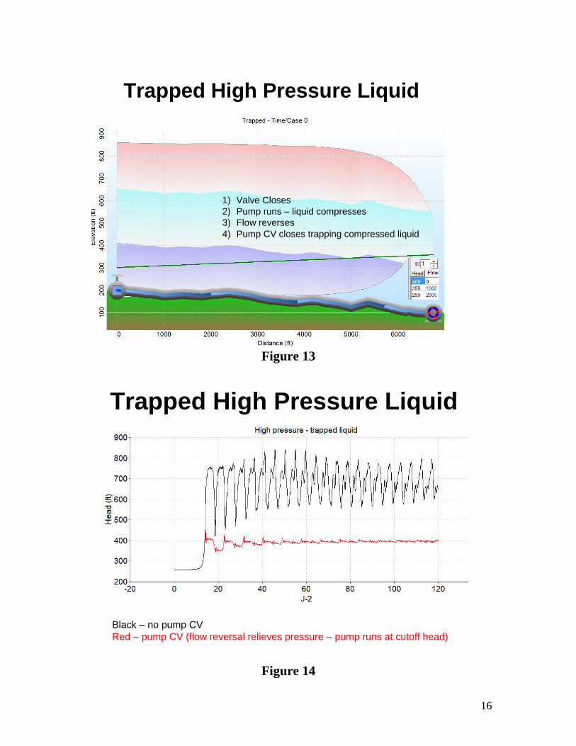
Trapped High Pressure Liquid

Black – no pump CV

Red – pump CV (flow reversal relieves pressure – pump runs at cutoff head)

Figure 14

17

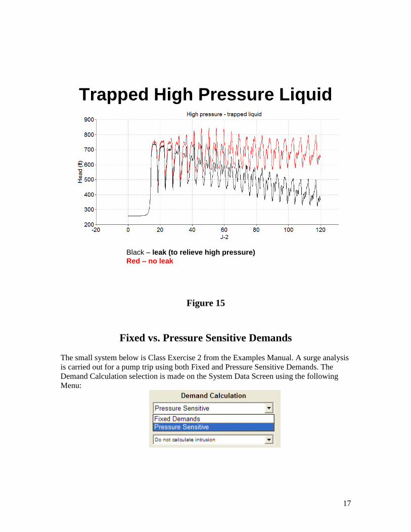
Trapped High Pressure Liquid

Black – leak (to relieve high pressure)

Red – no leak

Figure 15

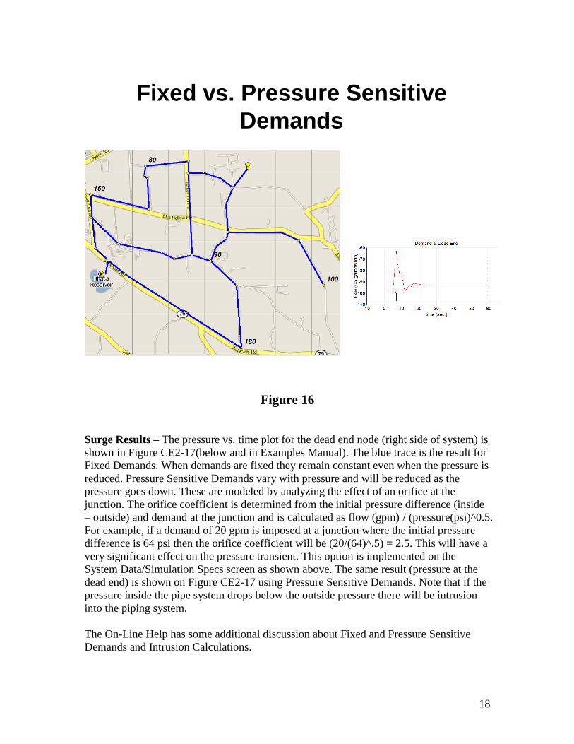
Fixed vs. Pressure Sensitive Demands

The small system below is Class Exercise 2 from the Examples Manual. A surge analysis

is carried out for a pump trip using both Fixed and Pressure Sensitive Demands. The

Demand Calculation selection is made on the System Data Screen using the following

Menu:

18

Fixed vs. Pressure Sensitive

Demands

Figure 16

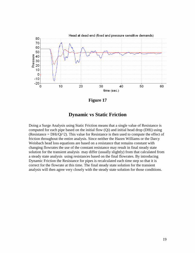
Surge Results – The pressure vs. time plot for the dead end node (right side of system) is

shown in Figure CE2-17(below and in Examples Manual). The blue trace is the result for

Fixed Demands. When demands are fixed they remain constant even when the pressure is

reduced. Pressure Sensitive Demands vary with pressure and will be reduced as the

pressure goes down. These are modeled by analyzing the effect of an orifice at the

junction. The orifice coefficient is determined from the initial pressure difference (inside

– outside) and demand at the junction and is calculated as flow (gpm) / (pressure(psi)^0.5.

For example, if a demand of 20 gpm is imposed at a junction where the initial pressure

difference is 64 psi then the orifice coefficient will be (20/(64)^.5) = 2.5. This will have a

very significant effect on the pressure transient. This option is implemented on the

System Data/Simulation Specs screen as shown above. The same result (pressure at the

dead end) is shown on Figure CE2-17 using Pressure Sensitive Demands. Note that if the

pressure inside the pipe system drops below the outside pressure there will be intrusion

into the piping system.

The On-Line Help has some additional discussion about Fixed and Pressure Sensitive

Demands and Intrusion Calculations.

19

Figure 17

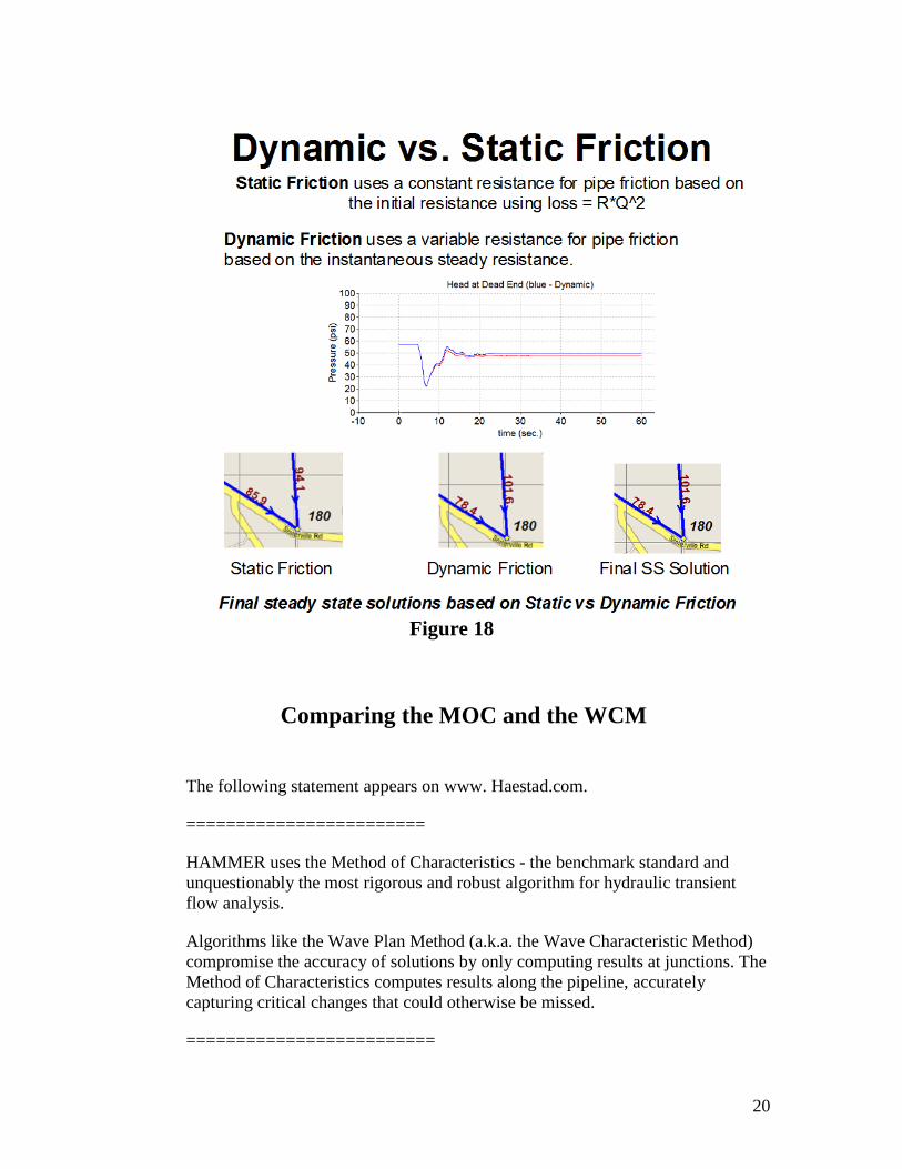
Dynamic vs Static Friction

Doing a Surge Analysis using Static Friction means that a single value of Resistance is

computed for each pipe based on the initial flow (Qi) and initial head drop (DHi) using

(Resistance = DHi/Qi^2). This value for Resistance is then used to compute the effect of

friction throughout the entire analysis. Since neither the Hazen Williams or the Darcy

Weisbach head loss equations are based on a resistance that remains constant with

changing flowrates the use of the constant resistance may result in final steady state

solution for the transient analysis may differ (usually slightly) from that calculated from

a steady state analysis using resistances based on the final flowrates. By introducing

Dynamic Friction the Resistance for pipes is recalculated each time step so that it is

correct for the flowrate at this time. The final steady state solution for the transient

analysis will then agree very closely with the steady state solution for those conditions.

20

Figure 18

Comparing the MOC and the WCM

The following statement appears on www. Haestad.com.

========================

HAMMER uses the Method of Characteristics - the benchmark standard and

unquestionably the most rigorous and robust algorithm for hydraulic transient

flow analysis.

Algorithms like the Wave Plan Method (a.k.a. the Wave Characteristic Method)

compromise the accuracy of solutions by only computing results at junctions. The

Method of Characteristics computes results along the pipeline, accurately

capturing critical changes that could otherwise be missed.

=========================

21

The above statements from Haestad’s www site is misleading and just plain wrong. The

following items address the issue of the Method of Characteristics (MOC) vs. the Wave

Characteristic Method (WCM) methods of transient analysis. The above statement

appears to be an attempt to put a positive spin on an enormous disadvantage of the MOC

– the computational inefficiency of the MOC technique.

1) An acceptable technique for solving the basic pipe system momentum and

continuity transient flow equations produces a correct solution. Since the solution

techniques are not exact mathematical solutions a correct solution is one which

satisfies all the basic equations and boundary conditions with an acceptable

degree of accuracy. Although there are multiple techniques for obtaining a

solution there is only one correct solution for a given problem. The concept that

one viable technique (MOC) is more rigorous and robust than another (WCM) is

nonsense since they both produce essentially the same result. The fact that the

MOC and the WCM produce the same result is documented in several technical

journal articles (listed at end of this section)

2) The efficiency of the solution technique used is an entirely different concept.

Certainly different computational procedures can be used to obtain the correct

solution and the WCM happens to be orders of magnitude more computationally

efficient than the MOC. This is particularly important because transient flow

analysis in a sizable piping system requires an extremely large number of

computations and an efficient algorithm is necessary to handle larger piping

systems in a timely manner

3) The implication that the WCM compromises accuracy because it computes results

only at junctions is also flawed. The WCM computes results at all devices in the

system and at junctions and any desired additional location. Good pipe system

modeling (steady state and transient) always dictates that modeling nodes are

placed at critical high and low points which are normally the only points of real

concern along a pipeline. No engineer would suggest that we add a node every

20-40 feet in every pipe in the steady state pipe system model because we might

miss a critical event. This would add great difficulty and overhead to the

modeling and analysis and rarely (if ever) provide any additional useful

information. Yet this is exactly what the above statement implies

4) It needs to be stressed that the only transient event (critical change referred to in

the above statement) occurring within a pipeline which affects the results is the

formation and analysis of a vapor cavity. Vapor cavities normally occur at a

device such as a pump or valve. When they occur within a pipeline they normally

form at local high points. As noted above good modeling will place a node and

define the elevation at local high points within the pipeline. An accurate

prediction of this event within a pipeline requires that the elevation of the location

is known precisely. A difference of just a few feet will compromise this

calculation. MOC models normally interpolate elevations at interior points. This

approximation will affect the accuracy of the prediction of the formation of a

vapor cavity – the critical change referred to in the above statement. Certainly

22

nodes placed precisely at high points will adequately predict the occurance of

cavitation.

5) The WCM technique for solving transient flow in piping systems requires that

solutions be calculated at all nodes (pumps, valves, etc), junctions, and additional

nodes (if any) inserted at critical locations. The MOC technique makes the same

calculations plus many additional required ones at numerous internal locations.

The MOC technique requires these internal calculations to handle the wave

propagation and frictional effects. Pressure wave action is incorporated into the

WCM method to handle the wave propagation and the effects of wall friction and

requires just one additional calculation for each pipe section. The result of this is

that the MOC usually requires order of magnitudes more calculations than does

the WCM to obtain the same solution. Because calculations are required at small

time increments (often .01 seconds or less) and simulations of 60 to 300 or more

seconds may be necessary, millions of calculations are often needed. Using a

technique which increases this requirement by orders of magnitude to get the

same result doesn’t make much sense. Even with modern fast computers the time

requirements for handling many water distribution systems could be very

significant (1 minute (WCM) vs 45 minutes (MOC), for example). Interestingly,

the Method of Characteristics was originally developed for solving open channel

transient flow problems with relatively slow moving pressure waves (compared to

the fast wave speeds of closed conduit flows) and that speaks volumes about the

inefficiency of MOC method when applied to closed conduit flows.

Boulos, P. F., Wood, D.J. and Funk, J.E. "A Comparison of Numerical and Exact Solutions for

Pressure Surge Analysis," Chapter 12, Proceedings, 6th International Conference on Pressure

Surges, Cambridge, England, Oct. 1989, pp. 149-159.

Wood, D.J.; Lingireddy, S., and Boulos, P.F., 2004 Pressure Wave Analysis Of Transient Flow In

Pipe Distribution Systems, MWHSoft Inc. Pasadena, CA. (2005)

Wood, D.J.; Lingireddy, S., Boulos, P.F., Karney B. W. and McPherson, D. L. Numerical

Methods for Modeling Transient Flow in Distribution Systems, Journal AWWA, July 2005

23

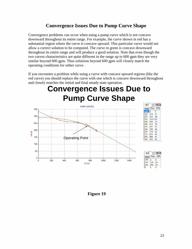
Convergence Issues Due to Pump Curve Shape

Convergence problems can occur when using a pump curve which is not concave

downward throughout its entire range. For example, the curve shown in red has a

substantial region where the curve is concave upward. This particular curve would not

allow a correct solution to be computed. The curve in green is concave downward

throughout its entire range and will produce a good solution. Note that even though the

two curves characteristics are quite different in the range up to 600 gpm they are very

similar beyond 600 gpm. Thus solutions beyond 600 gpm will closely match the

operating conditions for either curve.

If you encounter a problem while using a curve with concave upward regions (like the

red curve) you should replace the curve with one which is concave downward throughout

and closely matches the initial and final steady state operation.

Convergence Issues Due to

Pump Curve Shape

Operating Point

Figure 19

24

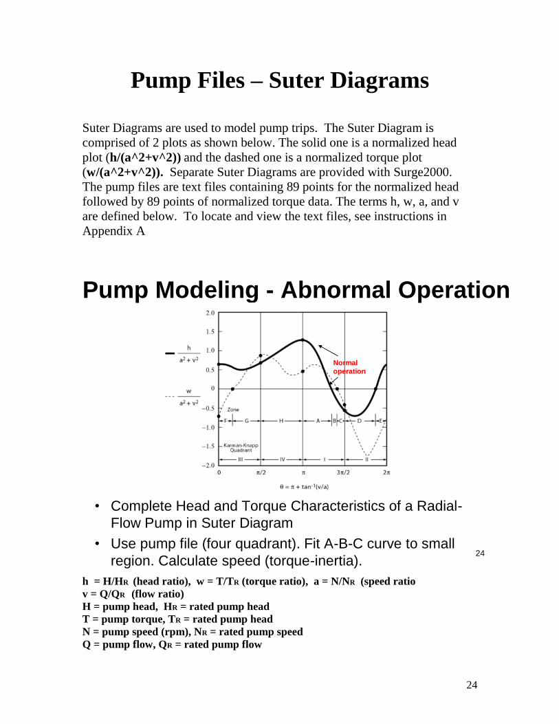
Pump Files – Suter Diagrams

Suter Diagrams are used to model pump trips. The Suter Diagram is

comprised of 2 plots as shown below. The solid one is a normalized head

plot (h/(a^2+v^2)) and the dashed one is a normalized torque plot

(w/(a^2+v^2)). Separate Suter Diagrams are provided with Surge2000.

The pump files are text files containing 89 points for the normalized head

followed by 89 points of normalized torque data. The terms h, w, a, and v

are defined below. To locate and view the text files, see instructions in

Appendix A

24

Pump Modeling - Abnormal Operation

• Complete Head and Torque Characteristics of a Radial-

Flow Pump in Suter Diagram

• Use pump file (four quadrant). Fit A-B-C curve to small

region. Calculate speed (torque-inertia).

Normal

operation

h = H/HR (head ratio), w = T/TR (torque ratio), a = N/NR (speed ratio

v = Q/QR (flow ratio)

H = pump head, HR = rated pump head

T = pump torque, TR = rated pump head

N = pump speed (rpm), NR = rated pump speed

Q = pump flow, QR = rated pump flow

25

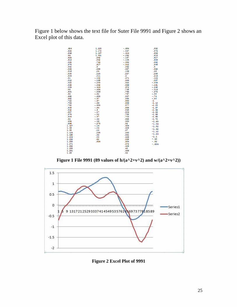
Figure 1 below shows the text file for Suter File 9991 and Figure 2 shows an

Excel plot of this data.

Figure 1 File 9991 (89 values of h/(a^2+v^2) and w/(a^2+v^2))

Figure 2 Excel Plot of 9991

26

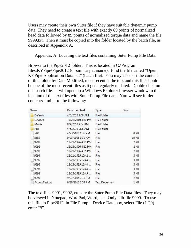
Users may create their own Suter file if they have suitable dynamic pump

data. They need to create a text file with exactly 89 points of normalized

head data followed by 89 points of normalized torque data and name the file

9999.txt. Then it must be copied into the folder located by the batch file, as

described in Appendix A.

Appendix A: Locating the text files containing Suter Pump File Data.

Browse to the Pipe2012 folder. This is located in C:\Program

files\KYPipe\Pipe2012 (or similar pathname). Find the file called “Open

KYPipe Application Data.bat” (batch file). You may also sort the contents

of this folder by Date Modified, most recent at the top, and this file should

be one of the most recent files as it gets regularly updated. Double click on

this batch file. It will open up a Windows Explorer browser window to the

location of the text files with Suter Pump File data. You will see folder

contents similar to the following:

The text files 9991, 9992, etc. are the Suter Pump File Data files. They may

be viewed in Notepad, WordPad, Word, etc. Only edit file 9999. To use

this file in Pipe2012, in File Pump – Device Data box, select File (1-20)

enter “9”.

27

Using Control Valves for Surge Protection

Suppose you need to shut down the flow in a pipeline in a specified period of time. This

action will always cause a pressure surge related to the deceleration of the fluid in the

pipeline. The type of valve you use and how it is operated can have a very significant

effect on the magnitude of the pressure surge and can provide protection against the

development of an excessive pressure surge.

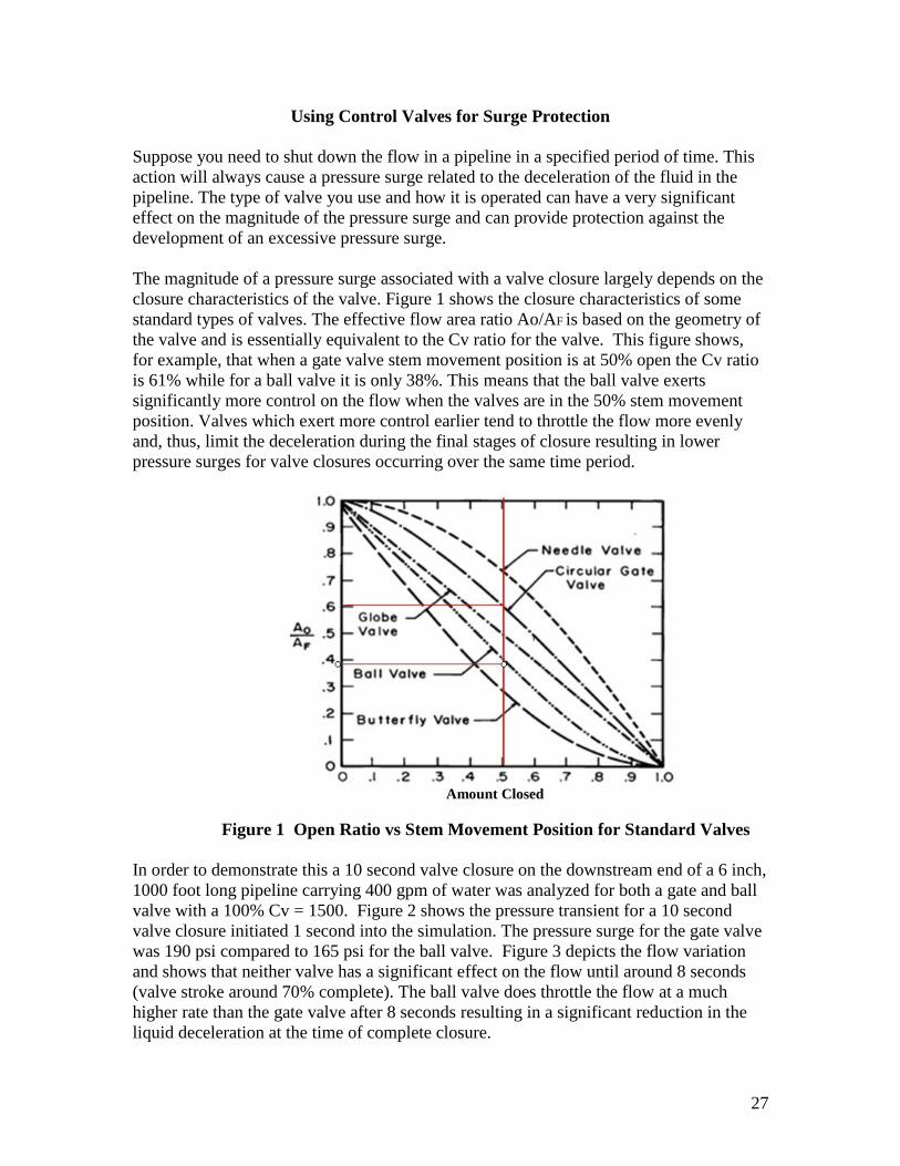
The magnitude of a pressure surge associated with a valve closure largely depends on the

closure characteristics of the valve. Figure 1 shows the closure characteristics of some

standard types of valves. The effective flow area ratio Ao/AF is based on the geometry of

the valve and is essentially equivalent to the Cv ratio for the valve. This figure shows,

for example, that when a gate valve stem movement position is at 50% open the Cv ratio

is 61% while for a ball valve it is only 38%. This means that the ball valve exerts

significantly more control on the flow when the valves are in the 50% stem movement

position. Valves which exert more control earlier tend to throttle the flow more evenly

and, thus, limit the deceleration during the final stages of closure resulting in lower

pressure surges for valve closures occurring over the same time period.

Amount Closed

Figure 1 Open Ratio vs Stem Movement Position for Standard Valves

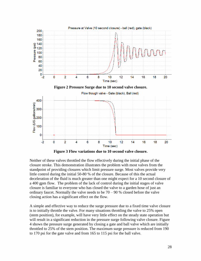
In order to demonstrate this a 10 second valve closure on the downstream end of a 6 inch,

1000 foot long pipeline carrying 400 gpm of water was analyzed for both a gate and ball

valve with a 100% Cv = 1500. Figure 2 shows the pressure transient for a 10 second

valve closure initiated 1 second into the simulation. The pressure surge for the gate valve

was 190 psi compared to 165 psi for the ball valve. Figure 3 depicts the flow variation

and shows that neither valve has a significant effect on the flow until around 8 seconds

(valve stroke around 70% complete). The ball valve does throttle the flow at a much

higher rate than the gate valve after 8 seconds resulting in a significant reduction in the

liquid deceleration at the time of complete closure.

28

Figure 2 Pressure Surge due to 10 second valve closure.

Figure 3 Flow variations due to 10 second valve closure.

Neither of these valves throttled the flow effectively during the initial phase of the

closure stroke. This demonstration illustrates the problem with most valves from the

standpoint of providing closures which limit pressure surge. Most valves provide very

little control during the initial 50-80 % of the closure. Because of this the actual

deceleration of the fluid is much greater than one might expect for a 10 second closure of

a 400 gpm flow. The problem of the lack of control during the initial stages of valve

closure is familiar to everyone who has closed the valve to a garden hose of just an

ordinary faucet. Normally the valve needs to be 70 – 90 % closed before the valve

closing action has a significant effect on the flow.

A simple and effective way to reduce the surge pressure due to a fixed time valve closure

is to initially throttle the valve. For many situations throttling the valve to 25% open

(stem position), for example, will have very little effect on the steady state operation but

will result in a significant reduction in the pressure surge following valve closure. Figure

4 shows the pressure surge generated by closing a gate and ball valve which are initially

throttled to 25% of the stem position. The maximum surge pressure is reduced from 190

to 170 psi for the gate valve and from 165 to 115 psi for the ball valve.

29

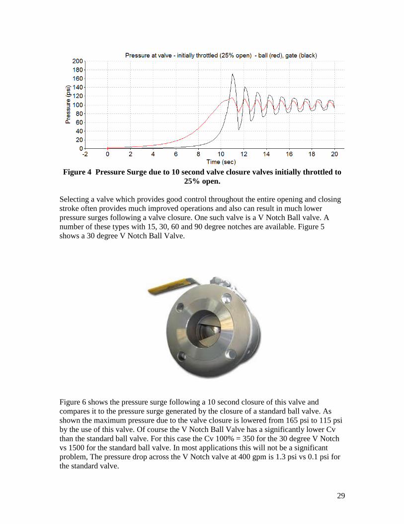
Figure 4 Pressure Surge due to 10 second valve closure valves initially throttled to

25% open.

Selecting a valve which provides good control throughout the entire opening and closing

stroke often provides much improved operations and also can result in much lower

pressure surges following a valve closure. One such valve is a V Notch Ball valve. A

number of these types with 15, 30, 60 and 90 degree notches are available. Figure 5

shows a 30 degree V Notch Ball Valve.

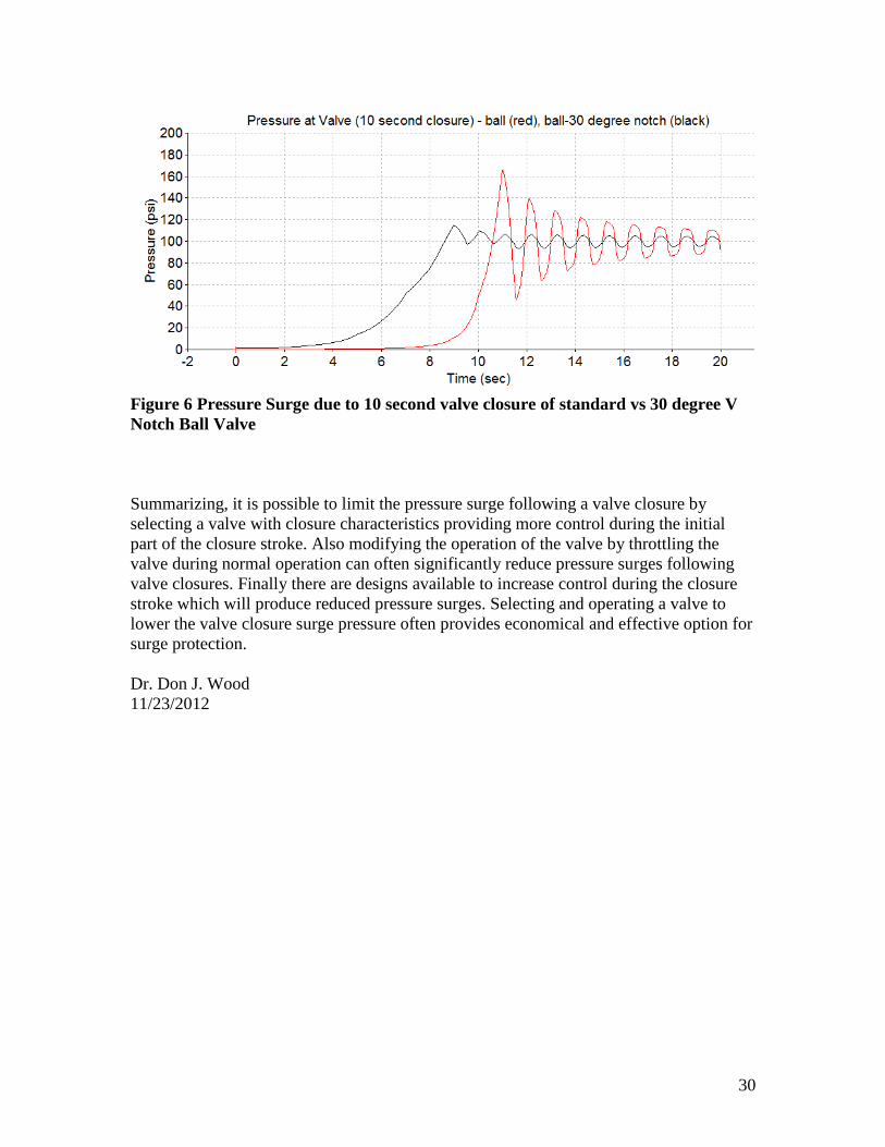
Figure 6 shows the pressure surge following a 10 second closure of this valve and

compares it to the pressure surge generated by the closure of a standard ball valve. As

shown the maximum pressure due to the valve closure is lowered from 165 psi to 115 psi

by the use of this valve. Of course the V Notch Ball Valve has a significantly lower Cv

than the standard ball valve. For this case the Cv 100% = 350 for the 30 degree V Notch

vs 1500 for the standard ball valve. In most applications this will not be a significant

problem, The pressure drop across the V Notch valve at 400 gpm is 1.3 psi vs 0.1 psi for

the standard valve.

30

Figure 6 Pressure Surge due to 10 second valve closure of standard vs 30 degree V

Notch Ball Valve

Summarizing, it is possible to limit the pressure surge following a valve closure by

selecting a valve with closure characteristics providing more control during the initial

part of the closure stroke. Also modifying the operation of the valve by throttling the

valve during normal operation can often significantly reduce pressure surges following

valve closures. Finally there are designs available to increase control during the closure

stroke which will produce reduced pressure surges. Selecting and operating a valve to

lower the valve closure surge pressure often provides economical and effective option for

surge protection.

Dr. Don J. Wood

11/23/2012