Surface roughness inspection by computer vision in turning operations

International Journal of Machine Tools & Manufacture 41 (2001) 1251–1263

Surface roughness inspection by computer vision in turningoperations

B.Y. Lee a, Y.S. Tarng b,*

a Department of Mechanical Manufacture Engineering, National Huwei Institute of Technology, Yunlin 642, Taiwan,ROC

b Department of Mechanical Engineering, National Taiwan University of Science and Technology, Taipei 106,Taiwan, ROC

Received 6 November 2000; accepted 26 January 2001

Abstract

The use of computer vision techniques to inspect surface roughness of a workpiece under a variationof turning operations has been reported in this paper. The surface image of the workpiece is first acquiredusing a digital camera and then the feature of the surface image is extracted. A polynomial network usinga self-organizing adaptive modeling method is applied to constructing the relationships between the featureof the surface image and the actual surface roughness under a variation of turning operations. As a result,the surface roughness of the turned part can be predicted with reasonable accuracy if the image of theturned surface and turning conditions are given. 2001 Published by Elsevier Science Ltd.

Keywords: Inspection; Surface roughness; Computer vision; Polynomial networks

1. Introduction

Turning is a widely used machining operation in the manufacturing process. Surface finishquality of workpiece is an issue of main concern to the manufacturing industry [1] and the inspec-tion of surface roughness of the workpiece is a very important technology. Basically, surfaceroughness measurements can be divided into two approaches: direct and indirect contact methods.Direct contact method depends on using stylus instruments, which require direct contact with thesurface to be investigated. Stylus instruments have limited flexibility in handling the differentgeometrical parts to be measured. In addition to this, measurement speed of the stylus instrument

* Corresponding author. Tel.: +886-2-2737-6456; fax: +886-2-737-6460.E-mail address: [email protected] (Y.S. Tarng).

0890-6955/01/$ - see front matter 2001 Published by Elsevier Science Ltd.PII: S0 890- 695 5(01 )000 23- 2

1252 B.Y. Lee, Y.S. Tarng / International Journal of Machine Tools & Manufacture 41 (2001) 1251–1263

is also slow. In contrast, the indirect method uses optical instruments which are inherently non-contact measurements and easy to automate. In this paper, an indirect method using computervision for inspecting surface roughness in turning has been developed.

In past decades, computer vision technology has maintained tremendous vitality in a lot offields. New applications continue to be found and existing applications to expand. Several investi-gations have been performed to inspect surface roughness of a workpiece based on computervision technology [2–6]. Although it has been shown that the surface roughness of a workpieceis strongly characterized by the surface image, practical surface roughness instruments based oncomputer vision technology are still difficult. The main obstacle is how to process the surfaceimage to obtain the actual surface roughness of workpiece, and this problem requires furtherresearch effect, especially under various cutting operations. In this paper, a self-organizing adapt-ive learning tool, called polynomial network [7], has been used to establish the relationshipsbetween the actual surface roughness of a workpiece and the feature of surface image under avariety of cutting operations. It has been shown that the polynomial network has great represen-tational power for dealing with highly nonlinear, strongly coupled, multivariable systems [8–11].As a result, the relationships between the actual surface roughness of the workpiece and thefeature of surface image under a variation of cutting operations can be constructed based on apolynomial network.

The paper is organized in the following manner. Measurement of the surface image of a work-piece is described first. The theory of polynomial networks is introduced next. Then, the use ofpolynomial networks to predict surface roughness of a workpiece under a variety of cutting oper-ations is shown. Finally, experimental verification of this approach is given.

2. Measurement of the surface image of a workpiece

A schematic diagram of the computer vision system for inspecting surface roughness in turningoperations is shown in Fig. 1. First, an appropriate light source is arranged to illuminate thesurface image of the workpiece. The surface image of a workpiece is acquired using a digitalcamera (Olympus C-1400L) and then transferred to the PC workstation through frame buffers.

Fig. 1. Schematic diagram of the computer vision system for inspecting surface roughness.

1253B.Y. Lee, Y.S. Tarng / International Journal of Machine Tools & Manufacture 41 (2001) 1251–1263

The digital camera captures the surface image with 1280×1024 resolution, 1/30 s grabbing speedand 8 bit digit output.

To investigate surface roughness under different cutting conditions, a number of cutting testswere carried out using a CNC lathe with a tungsten carbide tool and working on S45C steel bars.Experimental data with regard to different cutting parameters (cutting speed, feed rate and depthof cut) were performed. The feasible spaces of the cutting parameters were selected by varyingcutting speed V in the range 53.44–199.49 m/min, feed rate F in the range 0.06–0.52 mm/rev,depth of cut D in the range 0.5–1.5 mm. Fifty-seven turning experiments were performed basedon the cutting parameter combinations (Table 1).

Machined surface roughness was measured by a profile meter (Surfcorder SE-1100) within asampling length of 8 mm and measurement speed of 0.5 mm/s. The average surface roughnessRa that is the most widely used surface finish parameter in industry is selected in this study. Itis the arithmetic average of the absolute value of the heights of roughness irregularities from themean value measured, that is:

Ra�1n�

n

i�1

|yi| (1)

where yi is the height of roughness irregularities from the mean value and n is the number ofsampling data.

In this study, a feature of the surface image, called the arithmetic average of the grey levelGa, is used to predict the actual surface roughness of the workpiece. The arithmetic average ofthe grey level Ga can be expressed as:

Ga�1n�

n

i�1

|gi| (2)

where gi is the grey level of surface image deviated from the mean grey value.An example of how to obtain the arithmetic average of the grey level Ga from a surface image

is shown in Fig. 2. Fig. 2(a) displays the grey level of the surface image acquired by the digitalcamera and only the grey value along the dashed line is extracted. The grey level of the dashedline gi deviated from the mean grey value (Fig. 2(b)) is then calculated. Finally, the arithmeticaverage of the grey level Ga can be obtained using Eq. (2). The arithmetic average of the surfaceroughness Ra and the arithmetic average of the grey level Ga for the surface image correspondingto 57 turning experiments are summarized and also listed in Table 1. In the next section, thepolynomial network is used to establish the relationships between the actual surface roughness ofthe workpiece Ra and the feature of the surface image Ga under a variation of cutting operations.

3. Modeling of surface roughness based on the polynomial network

Polynomial networks proposed by Ivakhnenko [12] are a group method of data handling(GMDH) technique [13]. In a polynomial network, complex systems are decomposed into smaller,simpler subsystems and grouped into several layers using polynomial functional nodes. Inputs of


Tab

le1

Exp

erim

enta

ltu

rnin

gpa

ram

eter

san

dsu

rfac

ero

ughn

ess

for

trai

ning

test

s

Tes

tV

FD

Ga

Styl

usT

est

VF

DG

aSt

ylus

inst

rum

ent

inst

rum

ent

no.

(m/m

in)

(mm

/rev

)(m

m)

(gra

yle

vel)

Ra

(µm

)no

.(m

/min

)(m

m/r

ev)(

mm

)(g

ray

leve

l)R

a(µ

m)

153

.44

0.06

1.5

13.5

41.

454

3010

6.88

0.29

1.5

51.1

88.

332

253

.44

0.16

1.5

16.2

32.

213

3110

6.88

0.40

1.5

51.2

017

.90

353

.44

0.29

1.5

55.7

29.

625

3210

6.88

0.52

1.5

63.8

822

.72

453

.44

0.40

1.5

57.4

017

.16

3311

5.17

0.06

0.5

11.7

90.

882

553

.44

0.52

1.5

66.3

122

.25

3411

5.17

0.16

0.5

12.6

02.

184

657

.95

0.06

0.5

28.6

62.

375

3511

5.17

0.29

0.5

39.7

87.

176

757

.95

0.16

0.5

19.8

32.

525

3611

5.17

0.40

0.5

61.8

915

.97

857

.95

0.29

0.5

44.4

06.

6037

115.

170.

520.

554

.13

23.4

69

57.9

50.

400.

553

.44

14.4

238

119.

690.

061.

014

.51

0.82

510

57.9

50.

520.

575

.52

21.7

939

119.

690.

161.

013

.44

2.26

511

59.8

50.

061.

011

.86

1.66

4011

9.69

0.26

1.0

50.4

16.

713

1259

.85

0.16

1.0

14.5

22.

167

4111

9.69

0.40

1.0

59.5

85.

1313

59.8

50.

291.

056

.63

7.04

242

119.

690.

521.

063

.36

24.7

214

59.8

50.

521.

062

.83

25.7

043

178.

130.

061.

58.

751

0.71

715

75.7

00.

061.

515

.60

0.88

344

178.

130.

161.

517

.32

2.54

516

75.7

00.

161.

518

.40

2.46

545

178.

130.

291.

540

.11

9.03

417

75.7

00.

291.

552

.28

9.57

346

178.

130.

401.

554

.11

17.0

118

75.7

00.

401.

562

.68

15.0

547

178.

130.

521.

554

.26

23.2

619

75.7

00.

521.

570

.09

22.3

348

191.

950.

060.

512

.09

0.66

420

81.5

80.

060.

517

.99

0.82

449

191.

950.

160.

510

.78

2.16

121

81.5

80.

160.

513

.23

2.33

150

191.

950.

290.

542

.96

7.27

322

81.5

80.

290.

553

.48

6.81

551

191.

950.

400.

551

.50

15.0

823

81.5

80.

400.

564

.54

14.7

552

191.

950.

520.

556

.95

22.4

424

81.5

80.

520.

577

.20

23.1

553

199.

490.

061.

010

.94

0.88

725

84.7

80.

061.

013

.29

0.97

954

199.

490.

161.

014

.34

2.38

526

84.7

80.

161.

013

.45

1.87

155

199.

490.

291.

041

.28

7.02

627

84.7

80.

291.

053

.50

6.43

256

199.

490.

401.

051

.22

15.2

628

106.

880.

061.

59.

497

0.81

557

199.

490.

521.

062

.19

26.3

929

106.

880.

161.

513

.12

2.33

6


Fig. 2. An example of a surface image. (a) Grey level of the surface image. (b) Variations of the grey value alongthe dashed line (cutting speed, 119.69 m/min; feed rate, 0.4 mm/rev; depth of cut, 1.0 mm).

the network are subdivided into groups, then transmitted into individual functional nodes. Thesenodes evaluate the limited number of inputs by a polynomial function and generate an output toserve as an input to subsequent nodes of the next layer. The general methodology of dealing witha limited number of inputs at a time, then summarizing the input information, and then passingthe summarized information to a higher reasoning level is directly related to human behaviorsobserved by Miller [14]. Therefore, polynomial networks can be recognized as a special class ofbiologically inspired networks with machine intelligence and can be used effectively as a predictorfor estimating the outputs of complex systems.

3.1. Polynomial functional nodes

The general polynomial function known as the Ivakhnenko polynomial in a polynomial func-tional node can be expressed as:

y0�w0��mi�1

wixi��mi�1

�mj�1

wijxixj��mi�1

�mj�1

�mk�1

wijkxixjxk�… (3)

where xi, xj, xk are the inputs, y0 is the output, and w0, wi, wij, wijk are the coefficients of thepolynomial functional node.

In the present study, several specific types of polynomial functional nodes (Fig. 3) are used inthe polynomial network for the modeling of cutting performance in turning operations. An expla-nation of these polynomial functional nodes is given as follows.(i) Normalizer:A normalizer transforms the original input into the normalized input and the corresponding poly-nomial function can be expressed as:

y1�w0�w1x1 (4)


Fig. 3. Various polynomial functional nodes.

where x1 is the original input, y1 is the normalized input, and w0,w1 are the coefficients of the nor-malizer.

During this normalization process, the normalized input y1 is adjusted to have a mean of zeroand a variance of one.(ii) Unitizer:On the other hand, a unitizer converts the output of the network to the real output. The polynomialequation of the unitizer can be expressed as:

y1�w0�w1x1 (5)

where x1 is the output of the network, y1 is the real output, and w0,w1 are the coefficients ofthe unitizer.


The mean and variance of the real output must be equal to those of the output used to synthesizethe network.(iii) Single node:The single node only has one input and the polynomial equation is limited to the third degree,that is:

y1�w0�w1x1�w2x21�w3x3

1 (6)

where x1 is the input to the node, y1 is the output of the node, and w0,w1,w2 and w3 are thecoefficients of the single node.(vi) Double node:The double node takes two inputs at a time and the third-degree polynomial equation has thecross-term so as to consider the interaction between the two inputs, that is:

y1�w0�w1x1�w2x2�w3x21�w4x2

2�w5x1x2�w6x31�w7x3

2 (7)

where x1,x2 are the inputs to the node, y1 is the output of the node, and w0,w1,w2,%w7 are thecoefficients of the double node.(v) Triple node:Similar to the single and double nodes, the triple node with three inputs has more complicatedpolynomial equation allowing the interaction among these inputs, that is:

y1�w0�w1x1�w2x2�w3x3�w4x21�w5x2

2�w6x23�w7x1x2�w8x1x3�w9x2x3�w10x1x2x3 (8)

�w11x31�w12x3

2�w13x33

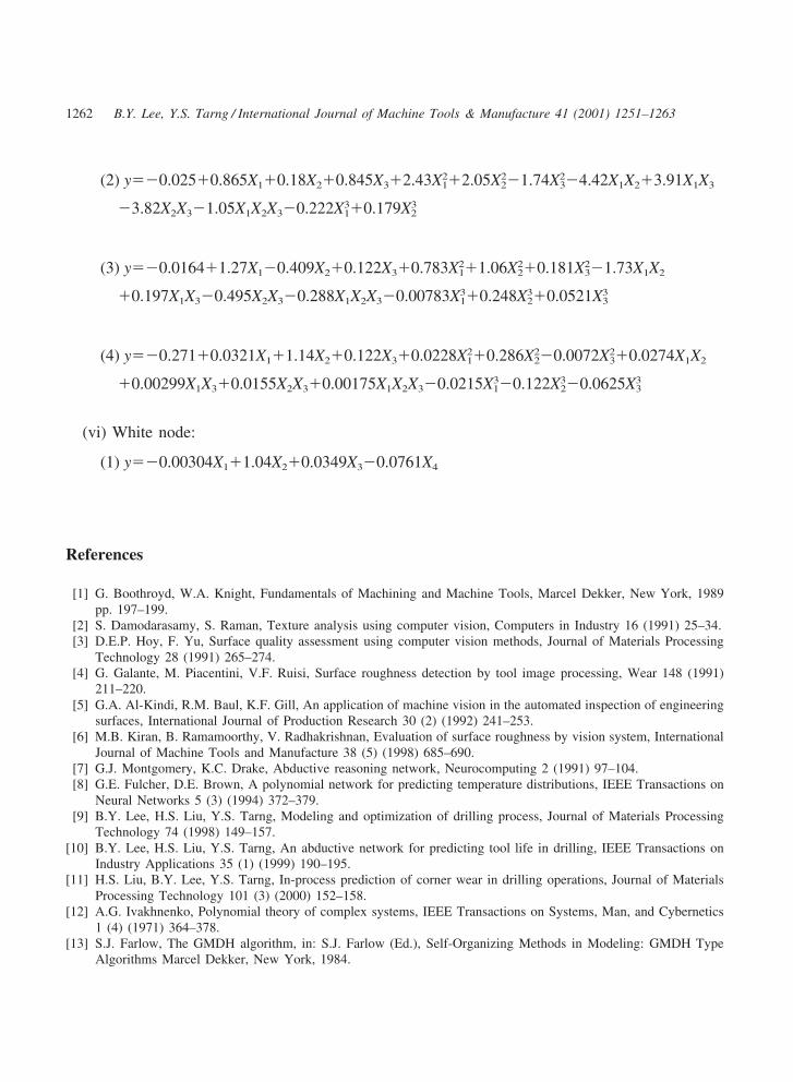
where x1,x2,x3 are the inputs to the node, y1 is the output of the node, and w0,w1,w2%w13 are thecoefficients of the triple node.(vi) White node:The white node is used to summarize all linear weighted inputs plus a constant, that is:

y1�w0�w1x1�w2x2�w3x3�…�wnxn (9)

where x1,x2,x3,…,xn are the inputs to the node, y1 is the output of the node, and w0,w1,w2,%wn

are the coefficients of the triple node.Since the functions of various polynomial functional nodes are explained, the next step is to

construct a polynomial network based on these functional nodes.

3.2. Synthesis of polynomial networks

To build a polynomial network, training samples with the information of inputs and outputsare required first (Table 1). Then, an algorithm for synthesis of polynomial networks (ASPN)[15] is used to determine an optimal network structure with the minimum value of the predictedsquared error (PSE) of the training samples. The PSE of the training samples is composed of twoterms, that is:

PSE�FSE�KP (10)

where FSE is the average squared error of the network for fitting the training data and KP is thecomplex penalty of the network.


The average squared error of the network FSE can be expressed as:

FSE�1N�

N

i�1

(yi�yi)2 (11)

where N is the number of training data, yi is the desired value in the training set, and yi is thepredicted value from the network.

The complex penalty of the network KP can be expressed as:

KP�CPM2s2

PKN

(12)

where CPM is the complex penalty multiplier, K is the number of coefficients in the network,and s2

P is a prior estimate of the model error variance, also equal to a prior estimate of FSE.As shown in Eq. (10), a trade-off between model accuracy and complexity is performed in the

ASPN criterion. This is because the principle of the ASPN criterion is to select a network asaccurate but as least complex as possible. In addition, the coefficient of CPM (Eq. (12)) can beused to adjust the trade-off. A complex network will be penalized more in the ASPN criterionas CPM is increased. In contrast, a complex network will be selected if CPM is decreased.

3.3. Prediction of surface roughness using the polynomial network

The polynomial network for predicting surface roughness can be constructed based on theexperimental data listed in Table 1. The input variables of the network are cutting speed V, feedrate F, depth of cut D, and the feature of surface image Ga. The output variable of the networkis then the predicted surface roughness Ra. The best network structure, number of layers, andfunctional node types can be determined using the ASPN criterion (Eqs. (10)–(12)). The flowchartfor the inspection of surface roughness proposed by this study is shown in Fig. 4. Fig. 5 showsthe developed polynomial network for predicting surface roughness. The polynomial equationsused in the network (Fig. 3) are listed in Appendix A. The predicted surface roughness Ra consist-ent with the measured surface roughness Ra is shown in Fig. 6. To further verify the predictionaccuracy of the polynomial network, several experiments were also performed (Table 2). A com-parison of the predicted surface roughness Ra and measured surface roughness Ra is shown inTable 2. It is shown that the polynomial network (Fig. 3) can be used to predict surface roughnesswith reasonable accuracy.

4. Conclusions

This paper has described the use of computer vision techniques to inspect the surface roughnessof a workpiece under various turning operations. The advantages of this approach are the non-contact measurements and ease of automation. A polynomial network with self-organized adaptivelearning ability is adopted in this study to process the surface image to obtain the surface rough-ness of the workpiece. It is shown that the polynomial network can correctly correlate the inputvariables (cutting speed, feed rate, depth of cut, and the feature of surface image) with the output


Fig. 4. Flowchart for the inspection of surface roughness based on the computer vision approach.

Fig. 5. Polynomial network for predicting surface roughness.


Fig. 6. Effect of the predicted surface roughness versus the measured surface roughness using training test data.

Table 2Experimental turning parameters and surface roughness for verification tests

Test V F D Vision Stylus instrument Errormeasurement

no. (m/min) (mm/rev) (mm) Ra (µm) Ra (µm) (%)

1 75.44 0.26 0.80 5.615 5.462 �2.82 75.44 0.32 0.80 8.123 8.140 0.23 75.44 0.35 0.80 10.801 11.710 7.84 75.44 0.45 0.80 21.457 19.890 �7.85 88.79 0.20 1.00 3.507 3.596 2.56 06.50 0.32 0.80 8.990 10.550 4.07 06.50 0.35 0.80 10.377 11.550 10.18 06.50 0.45 0.08 19.091 21.730 12.19 29.12 0.20 1.00 3.345 3.797 11.910 29.12 0.23 1.00 4.293 4.555 5.711 29.12 0.26 1.00 5.412 5.332 �1.512 77.50 0.32 1.20 9.652 11.230 14.013 77.50 0.35 0.80 10.819 11.280 4.014 77.50 0.45 1.20 20.529 20.060 �2.315 77.50 0.45 0.80 19.548 21.160 7.616 79.07 0.23 1.50 5.386 5.653 4.7


variable, surface roughness of the workpiece. As a result, experimental results have shown thatthe surface roughness of a turned part can be predicted with reasonable accuracy once the imageof the turned surface and turning conditions (cutting speed, feed rate, and depth of cut) are given,even under different turning operations.

Acknowledgements

Partially financial supported from the National Science Council of the Republic of China, Tai-wan under grant number NSC87-2216-E-011-025 is acknowledged with gratitude.

Appendix A

(i) Normalizer:

(1) y��1.68�6.05X1

(2) y��2.37�2.37X1

(3) y��1.47�0.0449X1

(4) y��2.18�0.00194X1

(ii) Unitizer:

(1) y�9.61�8.51X1

(iii) Single node:

(1) y��0.11�0.0366X1�0.112X21

(iv) Double node:

(1) y��0.61�0.493X1�1.2X2�0.202X21�0.576X2

2�0.227X1X2�0.231X31�0.167X3

2

(v) Triple node:

(1) y��0.249�1.29X1�0.0975X2�0.11X3�0.387X21�0.00458X2

2�0.0362X23�0.00791X1X2

�0.157X1X3�0.0207X2X3�0.0696X1X2X3�0.161X31


(2) y��0.025�0.865X1�0.18X2�0.845X3�2.43X21�2.05X2

2�1.74X23�4.42X1X2�3.91X1X3

�3.82X2X3�1.05X1X2X3�0.222X31�0.179X3

2

(3) y��0.0164�1.27X1�0.409X2�0.122X3�0.783X21�1.06X2

2�0.181X23�1.73X1X2

�0.197X1X3�0.495X2X3�0.288X1X2X3�0.00783X31�0.248X3

2�0.0521X33

(4) y��0.271�0.0321X1�1.14X2�0.122X3�0.0228X21�0.286X2

2�0.0072X23�0.0274X1X2

�0.00299X1X3�0.0155X2X3�0.00175X1X2X3�0.0215X31�0.122X3

2�0.0625X33

(vi) White node:

(1) y��0.00304X1�1.04X2�0.0349X3�0.0761X4

References

[1] G. Boothroyd, W.A. Knight, Fundamentals of Machining and Machine Tools, Marcel Dekker, New York, 1989pp. 197–199.

[2] S. Damodarasamy, S. Raman, Texture analysis using computer vision, Computers in Industry 16 (1991) 25–34.[3] D.E.P. Hoy, F. Yu, Surface quality assessment using computer vision methods, Journal of Materials Processing

Technology 28 (1991) 265–274.[4] G. Galante, M. Piacentini, V.F. Ruisi, Surface roughness detection by tool image processing, Wear 148 (1991)

211–220.[5] G.A. Al-Kindi, R.M. Baul, K.F. Gill, An application of machine vision in the automated inspection of engineering

surfaces, International Journal of Production Research 30 (2) (1992) 241–253.[6] M.B. Kiran, B. Ramamoorthy, V. Radhakrishnan, Evaluation of surface roughness by vision system, International

Journal of Machine Tools and Manufacture 38 (5) (1998) 685–690.[7] G.J. Montgomery, K.C. Drake, Abductive reasoning network, Neurocomputing 2 (1991) 97–104.[8] G.E. Fulcher, D.E. Brown, A polynomial network for predicting temperature distributions, IEEE Transactions on

Neural Networks 5 (3) (1994) 372–379.[9] B.Y. Lee, H.S. Liu, Y.S. Tarng, Modeling and optimization of drilling process, Journal of Materials Processing

Technology 74 (1998) 149–157.[10] B.Y. Lee, H.S. Liu, Y.S. Tarng, An abductive network for predicting tool life in drilling, IEEE Transactions on

Industry Applications 35 (1) (1999) 190–195.[11] H.S. Liu, B.Y. Lee, Y.S. Tarng, In-process prediction of corner wear in drilling operations, Journal of Materials

Processing Technology 101 (3) (2000) 152–158.[12] A.G. Ivakhnenko, Polynomial theory of complex systems, IEEE Transactions on Systems, Man, and Cybernetics

1 (4) (1971) 364–378.[13] S.J. Farlow, The GMDH algorithm, in: S.J. Farlow (Ed.), Self-Organizing Methods in Modeling: GMDH Type

Algorithms Marcel Dekker, New York, 1984.


[14] G.A. Miller, The magic number seven, plus or minus two: some limits on our capacity for processing information,The Psychological Review 63 (1956) 81–97.

[15] A.R. Barron, Predicted squared error: a criterion for automatic model selection, in: S.J. Farlow (Ed.), Self-Organiz-ing Methods in Modeling: GMDH Type Algorithms Marcel Dekker, New York, 1984.

Documents

Surface roughness inspection by computer vision in turning operations