Surface Ozone Variability and Trend over Urban and

Aerosol and Air Quality Research, 16: 138–152, 2016 Copyright © Taiwan Association for Aerosol Research ISSN: 1680-8584 print / 2071-1409 online doi: 10.4209/aaqr.2015.02.0113

Surface Ozone Variability and Trend over Urban and Suburban Sites in Portugal Pavan S. Kulkarni1*, Daniele Bortoli1,2, Ana Domingues1, Ana Maria Silva1,3 1 Instituto de Ciências da Terra (ICT), University of Évora, Évora, Portugal 2 Institute for Atmospheric Science and Climate (ISAC-CNR), Bologna, Italy 3 Department of Physics, University of Évora, Évora, Portugal ABSTRACT

The surface ozone time series is analyzed for the seasonal and inter-annual variations and the trend in the following three categories (a) monthly mean (b) 8 hr monthly mean and (c) daily maximum monthly mean measured at 8 (urban/suburban) sites in Portugal for the period 2000–2010. The inter-annual variation of the monthly mean surface ozone time series showed an year to year variation with the highest value in May 2009 (95 µg m–3) at Monte Chãos and the lowest in Jan 2002 (17 µg m–3) at Paio Pires. The trend analysis of (1) original surface ozone time series and of (2) deseasonalized surface ozone time series for all the three data set categories and for all the 8 sites was performed and found to be statistically significant at 6 sites for monthly mean and 8 hr monthly mean and at 5 sites for daily maximum monthly meanusing the non-parametric Mann-Kendall test. The analysis of original surface ozone time series showed a positive trend at 6 out of 8 sites, but the results were not statistically significant for most of the sites due to the presence of the annual cycle masking the actual trend values. However, the analysis of deseasonalized surface ozone time series showed a statistically significant increasing trend at 7 out of 8 sites with high Z values. The positive trends found in the deseasonalized surface ozone time series were in the range 0.44 up to 1.42 µg m–3 year–1 for the monthly mean surface ozone time series (7 stations), 0.33 up to 1.43 µg m–3 year–1 in the case of the 8 hr monthly mean surface ozone time series (7 stations) and 0.66 up to 1.55 µg m–3 year–1 in the daily maximum monthly mean surface ozone time series (6 stations). Keywords: Surface Ozone; Ozone variability; Ozone trend; Deseasonalization. INTRODUCTION

Surface ozone (O3) is a highly reactive trace gas and an important greenhouse gas (Mickley et al., 2001) which contributes to global warming and climate change (Unger et al., 2006). It is also a volatile secondary photochemical air pollutant and an important photochemical oxidant. Surface O3 affects adversely to the human health from its irritant properties and its induction of an inflammatory response in the lung. O3 also has adverse effects on crop yields and tree growth (Felzer et al., 2007; Premuda et al., 2013).

Increase in emission of O3 precursors such as nitrogen oxides (NOx), volatile organic compounds (VOC’s), carbon monoxide (CO) and non-methane hydrocarbons (NMHCs) (Saito et al., 2002) from traffic and industrial activities lead to increased production of surface O3 over polluted regions (Kulkarni et al., 2010). This is of great importance since O3 * Corresponding author.

Tel.: +351-266 740800; Fax: +351-266-745394 E-mail addresses: [email protected]; [email protected]

formed over source regions can then be transported over great distances affecting areas far from the source (Kulkarni et al., 2009; Kulkarni et al., 2011a, b). The build-up of surface O3 has broad implications on atmospheric chemistry and plays a significant role in controlling the chemical lifetimes and the reaction products of many atmospheric species. During sunlight hours, photochemical oxidation of VOCs initiated by hydroxyl radicals (OH) produces organic peroxy radicals (RO2), facilitating cycling of nitrogen oxide (NO) to nitrogen dioxide (NO2) and formation of surface O3 (Eqs. (1)–(4)) (Zhang et al., 2004; West et al., 2006). OH + VOC (+ O2) → RO2 (1) RO2 + NO → RO + NO2 (2) NO2 + hv → NO + O (3) O + O2 → O3 (4)

As solar zenith angle (SZA) decreases, from early morning till afternoon, production rate of O3 goes up and begins to accumulate in the atmosphere and reaches maximum concentration in the late afternoon. In the evening, with

Kulkarni et al., Aerosol and Air Quality Research, 16: 138–152, 2016 139

increasing SZA, O3 concentration starts declining and, after sunset, reaches its minimum around late night/early morning. At night, the photochemical process ceases, terminating chemical NOx removal such as by the reaction of OH with NO2 to form HNO3. Consequently, the large abundance of NOx near the surface level leads to the removal of O3 (Eq. (5)) (Zhang et al., 2004; West et al., 2006). NO + O3 → NO2 + O2 (5)

The Eqs. (1)–(5) along with O3 removal due to surface deposition (Pio et al., 2000) are primarily responsible for the diurnal variation of surface O3, with day time maxima and night time minima in the surface O3 concentration.

Surface O3 concentration in urban and suburban areas exhibits marked seasonal variability (Air Quality Expert Group-AQEG, 2009), with high concentration during the summer (due to high solar radiation and long sunlight hours) and low concentration during the winter (due to low solar radiation and short sunlight hours). However, in many rural environments the ozone seasonal peak may occur in spring, which may be due to the biogenic emissions in the rural regions leading to ozone formation. Apart from in-situ production of surface O3, long as well as short range transport of O3 and of O3 precursors, has an important impact on O3 concentrations at both regional and local scales. On the other hand, transport of O3 from the stratosphere to free troposphere, where mixing ratios are higher, and further into the boundary layer is another important source of surface O3 (Jain et al., 2005). Furthermore, O3 is formed in the free troposphere, especially in the northern hemisphere, mainly by the oxidation of methane (CH4) and also of CO (West et al., 2006; Ghude et al., 2011a, b) which, under favorable conditions, gets transported into the boundary layer. Besides temporal variability and transport mechanisms, variability in the meteorological conditions contributes to large inter-annual variability of surface O3 concentrations.

Surface O3 concentration at any given location can increase or decrease over a period of time and may give rise to a trend. Therefore one of the main goals of surface O3 concentration long term studies is the analysis of trends. The studies of seasonal and inter-annual variation as well as of trend analysis of surface O3 concentration are essential for formulating policy decisions on air quality.

Recent studies have shown an increasing trend of surface O3 over rural areas in Europe and over many urban and suburban sites all over the world. For example, Sicard et al. (2009) reported slight increase in annual averaged O3 concentrations in rural areas between 1995 and 2003 over France. Brönnimann et al. (2002) found increase in the monthly mean values in Switzerland in the 1990s. AQEG (2009) reported positive trend in the annual mean daily maximum 8-hour mean surface O3 at 48 sites out of 50 urban and roadside sites spread across the United Kingdom during the period from 1990 onwards and found that 18 of the 48 sites have statistically significant trend at 0.01(3 sites), 0.05 (7 sites) and 0.1 (8 sites) level of significance. The long term trend analysis of surface O3 performed by Fernández-Fernández et al. (2011) for the period 2001–

2007 over Iberian Peninsula, including one rural surface O3 monitoring site (Monte Velho) in Portugal, located at the Atlantic coast, observed increasing trend in the south of the Iberian Peninsula (IB) whereas decreasing trends were observed in the northern IB. Similarly, Monteiro et al. (2012) reported negative trends over eastern and northern Iberian Peninsula and positive trends over Atlantic coast, including two surface O3 monitoring site (Custóias and Paio Pires) in Portugal, for the period 2000–2009.

There have been various studies on the analysis of surface O3 using different statistical techniques in different regions of Portugal, particularly over northern Portugal (Pio et al., 2000; Pereira et al., 2005; Alvim-Ferraz et al., 2006; Sousa et al., 2009a; Carvalho et al., 2010; Sousa et al., 2010). Pereira et al. (2005) observed surface O3 exceedance of public information values and alert levels defined by air quality framework directive for Europe around Oporto region during the study period. Pio et al. (2000) carried out O3 dry deposition measurement in the northern Portugal during 1994–1995 and observed prominent diurnal and seasonal patterns in deposition flux, dry deposition velocity and surface resistance, especially for the daytime period. Alvim-Ferraz et al. (2006) compared surface O3 measurements from 1861–1897 with measurements from 2002–2003 period and found that these values are 147% higher than the ones obtained in the previous period 1861–1897, concluding that this increase is the result of enhanced photochemical production of O3 due to the growth in anthropogenic emissions. Monteiro et al. (2005) developed and validated a numerical air quality operational forecasting system over Portugal during the summer 2003 and noted that still improvements are needed on the chemistry-transport model. Sousa et al. (2009b; 2011) observed that occurrence of childhood asthmatic symptoms were significantly higher at sites with high surface O3 values than at sites with low surface O3 values.

Long term trend analysis of surface O3 time series is performed for one rural site (Monte Velho) (Fernández-Fernández et al., 2011) and two suburban sites (Custóias and Paio Pires) (Monteiro et al., 2012). However, the same was not done for any site using deseasonalized time series which is the suitable approach for analyzingstatistically significant trends of a given environmental quantity varying periodically with time (Carslaw, 2005). Moreover this type of analysis was also never done for urban/suburban background sites used in this study, with the exception of Paio Pires.

The objectives of this work were: (1) to study seasonal and inter-annual variation of surface O3 for the period 2000–2010 over urban and suburban sites in continental Portugal; (2) to analyze surface O3 time series and deseasonalized surface O3 time series for identifying possible existence of statistically significant trends over urban/suburban background sites in Portugal. DATA AND METHODOLOGY

Hourly records of surface O3 concentrations were obtained from 8 background sites representative of two categories: (A) urban background and suburban background close to urban centers i.e., to Lisbon metropolitan area and to Porto


metropolitan area, and (B) suburban background far from urban centers, spread over continental Portugal (see Fig. 1). All of these stations belong to the Environmental Portuguese Agency (APA-Agência Portuguesa do Ambiente) network. The APA is responsible for air pollution measurements at various stations all over Portugal in different type of environment (urban, suburban and rural) and of influence (background, traffic and industrial). The categorization of both types (environment and influence) is done by APA. The air quality data measured at the stations are sent to a central database for public display. The data then undergoes a validation and quality check before being archived on the website for further use. APA measures various pollutants but primarily uses five main pollutants for the calculation of the index of air quality, which are CO, NO2, sulfur dioxide (SO2), O3 and aerosols (measured as PM10). For further details about APA and its functioning please visit http://www.qualar.apambiente.pt/.

Table 1 provides a detailed list with information such as name of thestation, station code (used in this study), latitude-longitude-altitude coordinates, type of station (urban or suburban), temporal period and number of months of data used for trend analysis. Last column of Table 1 also shows, in parenthesis, percentage of number of months used for trend analysis with respect to the study period. Only days with more than 75% or with 18 hr of measurements (Air quality Directive 2008/50/EC) and months with more than 65% or 19 days of measurementsare used to compute monthly means for studying seasonal and inter-annual variations and trend analysis.

For simplification of analysis the aforementioned 8 sites can be broadly categorized into three regions namely, (a) Porto region: consisting of Ermesinde, VN da Telha and Leça do Balio monitoring sites, all within a radius of about 10 km, (b) Lisbon region: consisting of Beato, Alfragide and Paio Pires monitoring sites, all within a radius of about 15 km and (c) remaining sites: which include Teixugueira and Monte Chãos as depicted in Fig. 1. Lisbon is capital of Portugal and biggest metropolitan area with a population of 2,224,984 (Censes, 2011) with 0.58% growth since 2001. Lisbon region, comprising Lisbon Metropolitan area (LMA), is located in the western coast of Portugal (central part) close to the Atlantic Ocean with a complex coastline. To the north, there are Montejunto and Sintra hills reaching more than 400 m above sea level (a.s.l.). To the south, there are Arrábida hills (501 m) and the Sado estuary. The city of Lisbon is located at the northern side of Tagus river, near the Atlantic ocean. Tagus and Sado river (south of Lisbon Metropolitan area) valleys are the major orographic features (Barros et al., 2003). Lisbon and south of Lisbon has subtropical Mediterranean climate (Koppen-Geiger Climate Classification Csa) with mild winters and medium hot summers. Porto is the country’s second biggest metropolitan area, which has a population of 1,816,045 (Censes, 2011) with 0.082% relativegrowth since 2001. Porto region, comprising Porto Metropolitan area (PMA), is located in the northwest of Portugal, at the cross-section of Douro River and Atlantic Ocean (Madureira et al., 2011). Porto and the north of Porto with some part of central Portugal has Mediterranean climate (Koppen-Geiger Climate Classification

Fig. 1. Map of Portugal with location of Air Quality (ozone) monitoring sites (red dots) used in this study.

Csb) with humid warm summers and mild rainy winters. The remaining two sites are suburban and urban areas with combined population of less than 100,000 and are also located on the western coast of the Iberian Peninsula close to the Atlantic Ocean. All the O3 monitoring sites used in this study are located more or less within 50 km line of sight from the Atlantic Ocean. Peculiar orographic characteristics of each region lead to different local wind patterns in all the three regions, even under similar synoptic-scale conditions. The overall vehicular density in Portugal, particularly car, was 572 cars per 1000 inhabitants in 2003 (European Commission, DG-REGIO, 2006).

In this study, three different surface O3 time series were computed such as: (a) monthly mean, (b) daytime 8 hr monthly mean and (c) daily maxima monthly mean. The importance of computing monthly mean surface O3 values from hourly data helps in identifying seasonal variationsas well as trends and reflects the overall growth scenario (increasing or decreasing). On the other hand, the computing daily maximum monthly mean surface O3 values focuses on short exposure at a high level (Qin et al., 2004) and the monthly mean of daytime (1000 hr–1700 hr) 8 hr monthly mean value emphases on longer exposure at a moderate level (USEPA, 1996). Moreover several studies have shown


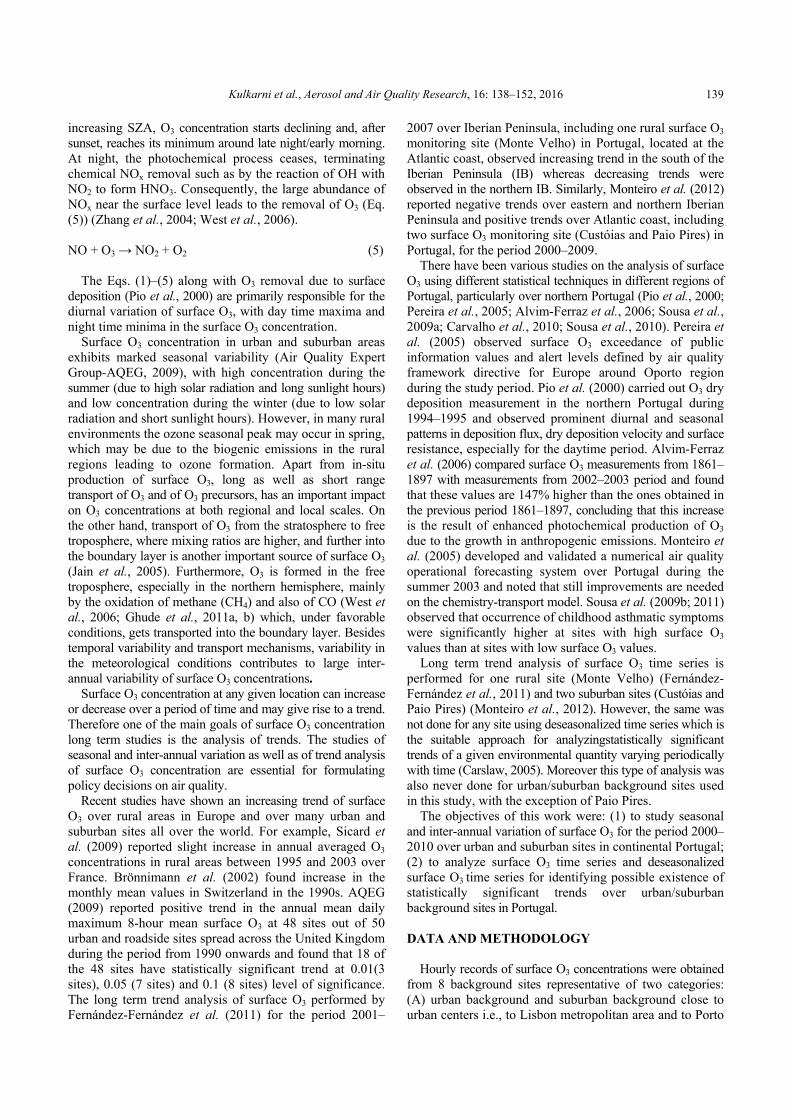
Table 1. Location of ozone monitoring sites, Lat; Long; Altitude, type, study period, No. of months data used for trend analysis (% w.r.t period).

Site Site code Lat; Long; Altitude Type* Period B(%) Beato B 38°53'41''; –9°07'03''; 56 U 2000–2010 132 (100)

Alfragide A 38°44'20''; –9°12'27''; 109 U 2001–2010 117 (97.5) Paio Pires PP 38°37'10''; –9°04'52''; 47 S 2001–2010 118 (98.3) Ermesinde E 41°12'24''; –8°33'10''; 140 U 2000–2010 130 (98.4)

Vila Nova da Telha VNT 41°15'08''; –8°39'38''; 88 S 2000–2010 126 (98.4) Leça do Balio LB 41°13'05''; –8°37'56''; 40 S 2000–2010 117 (88.6) Teixugueira T 40°45'24''; –8°34'22''; 20 S 2000–2010 124 (93.9)

Monte Chãos MC 37°57'15''; –8°50'17''; 129 S 2000–2010 123 (93.1) * All background sites (U-Urban; S-Suburban). B: –No. of months of data used for trend analysis.

that the new 8 hr O3 standard is more stringent than the 1 hr standard (Husar, 1996; Lefohn et al., 1998; Hogrefe et al., 2000; Velasco et al., 2000; Sather et al., 2001). Each surface O3 time series is analyzed for seasonal and inter-annual variations and to compute the long term trends.

The trend analysis was done on the original surface O3 time series and on the deseasonalized surface O3 time series. In both cases, first the linear O3 trend was derived from a simple linear regression analysis and secondly the statistical significance of the trend was tested with the non-parametric Mann-Kendall test. Simple linear regression is a technique in the parametric statistics that is commonly used for analyzing mean response of variable Y which changes according to the magnitude of an intervention variable X. It fits a straight line through the set of n points in such a way that makes the sum of squared residuals of the model as small as possible. The non-parametric Mann-Kendall test can be used to detect trends that are monotonic but not necessarily linear (Olofintoye and Sule, 2010) and is generally used in environmental science (AQEG 2009; De Leeuw, 2000). The null hypothesis in the Mann-Kendall test is that the data are independent and randomly ordered. The Mann-Kendall test does not require the assumption of normality, and only indicates the direction but not the magnitude of significant trends (McBean and Motiee, 2008). The Mann-Kendall test statistic S can be positive, negative or null. A very high positive value of S shows an increasing trend and a very low negative value shows a decreasing trend. However, it is necessary to compute the probability associated with S and the sample size, n, to statistically quantify the significance of the trend (Khambhammettu, 2005). The statistic test Z (which follow a normal distribution) has to be computed for a given level of significance, and in this study the 90% level of confidence (Z0.05 = 1.68) was used. The trend is increasing if Z is positive and greater than the level of significance and decreasing if Z is negative and the absolute value is greater than the level of significance. If the absolute value of Z is less than the level of significance, there is no significant trend (Khambhammettu, 2005). RESULTS AND DISCUSSION Seasonal and Inter-Annual Variation

The major component of surface O3 variation, both inter-

annual and seasonal, is its annual cycle (spring/summer maxima and winter minima), which is primarily controlled at macro level by solar insolation cycle, in-situ production and transport, which includes both long and short ranges. The annual cycle dominates in the monthly mean, the 8 hr monthly mean and the daily maximum monthly mean surface O3 time series values at any given location around the globe and the same was also observed at all the sites used in this study (Supporting Information SI1-Figs. 1(a), 1(b), 1(c): time series plots for all the 8 sites for each time series respectively). The high concentration of surface O3 during spring/summer is mainly due to high solar radiation and longer daylight hours, while comparatively low concentration of surface O3 during winter is due to low solar radiation and shorter daylight hours. Similarlythe type of environment, the type of influence (background, traffic or industrial) and pollutant transport also play a vital role.

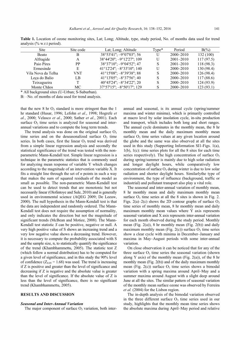
The seasonal and inter-annual variation of monthly mean, 8 hr monthly mean and daily maximum monthly mean surface O3 time series at all the 8 sites is shown in Fig. 2. Figs. 2(a)–2(c) shows the 2D contour graphs of surface O3 time series of monthly mean, 8 hr monthly mean and daily maximum monthly mean values where Y axis represents seasonal variation and X axis represents inter-annual variation for each month observed during the study period. Monthly mean (Fig. 2(a)), 8 hr monthly mean (Fig. 2(b)) and daily maximum monthly mean (Fig. 2(c)) surface O3 time series show a clear cycle with minima in December–January and maxima in May–August periods with some inter-annual variation.

On close observation it can be noticed that for any of the three surface O3 time series the seasonal variation (shown along Y axis) of the monthly mean (Fig. 2(a)), of the 8 hr monthly mean (Fig. 2(b)) and of the daily maximum monthly mean (Fig. 2(c)) surface O3 time series shows a bimodal variation with a spring maxima around April–May and a summer maxima around August with a slight deep around June at all the sites. The similar pattern of seasonal variation of the monthly mean surface ozone was observed by Ferreira et al. (2004) for the Lisbon region.

The in-depth analysis of the bimodal variation observed in the three different surface O3 time series used in our study, highlights that the monthly mean time series shows the absolute maxima during April–May period and relative


Fig. 2(a). Seasonal and year to year variation of monthly mean surface ozone concentration at different sites during the period 2000–2010 (2001–2010 for A and PP).

maximum values around August (Fig. 2(a)), whereas the bimodal variation observed for the 8 hr monthly mean and for the daily maximum monthly mean time series presents the relative maxima for the April–May period and the absolute maximum values in July–August period (Figs. 2(b) and 2(c)).

The spring maxima of surface O3 concentration in April–May period are probably due to more than one reason. Some of the known reasons can be the enhanced photochemistry after a winter accumulation of air pollutants (Penkett and Brice, 1986; Fernández-Fernández et al., 2011), Stratospheric-Tropospheric exchange of O3 which further intrudes into the boundary layer (Atlas et al., 2003), long and short range transport (Carvalho et al., 2010) and variability of meteorological parameters (Kulkarni et al., 2013). The summer maxima of surface O3 concentration in July–August seems to be due to high temperatures observed in the region during July–August period along with the variability in the number and in the magnitude of forest fires occurring in and around Portugal (Carvalho et al., 2011). Further, Ferreira et al. (2004) observed that high numbers of exceedances of the information threshold (180 µg m–3 -

one hour) are usually registered in July and August period. This confirms that the observed bimodal variation in the seasonal cycle of surface O3 with thespring maxima around April–May is mainly due to the dynamics of atmospheric processes in the atmospheric boundary layer and the summer maxima in July–August is due to the photochemical ozone generation (Tarasova et al., 2007; Zvyagintsev et al., 2008). Further, the spring relative maxima and the summer absolute maxima observed in the 8 hr monthly mean and in the daily maximum surface O3 time series is representative of day time photochemistry due to high solar radiation and temperature leading to high numbers of exceedances during the summer, whereas the spring absolute maxima and summer relative maxima observed in the monthly mean surface O3 time series is representative of the 24 hour average with longer nighttime period during spring compared to the summer time. In addition, Table 2 gives the statistical summary of minima, maxima and means (± Standard deviation) of monthly mean, 8 hr monthly mean and daily maximum monthly mean surface O3 time series at all the 8 sites during the study period.


Fig. 2(b). Seasonal and year to year variation of 8 hr monthly mean surface ozone concentration at different sites during the period 2000–2010 (2001–2010 for A and PP).

In Lisbon region, at Beato, Alfragide and Paio Pires stations, the observed monthly mean, 8 hr monthly mean and daily maximum monthly mean values of surface O3 for the study period are approximately the same (Table 2). The orographic features of Lisbon metropolitan region with Tagus and Sado river valleys trap the pollution and local circulation pattern may help toa better mixing of pollutants, which needs to be further validated. In Porto region, at the Ermesinde station the observed 8 hr monthly mean and daily maximum monthly meanvalues along with standard deviations are approximately the same (59 ± 17 µg m–3) which leads to the conclusion that surface O3 concentration remains more or less the same over the period of 8 h on most of the days and there are very few peak of O3 concentrations. However, at Vila Nova da Telha and Leça do Balio stations, which are suburban sites west of Ermesinde station and of Porto metropolitan area, lower 8 hr monthly mean surface O3 values are observed compared to the daily maximum monthly mean surface O3 values (Table 2). At Teixugueira and Monte Chãos, the observed maxima and mean values of monthly mean, 8 hr monthly mean and of daily maximum

monthly mean surface O3 concentration are more than over other urban/suburban sites (Table 2). The analysis of wind vectors was done (Supporting Information SI2-Fig. 2) using the European Centre for Medium-Range Weather Forecasts (ECMWF) ERA40 re-analysis data products (Uppala et al., 2005) with 1.125° horizontal resolution at 925 hPa over Portugal and adjacent area. The 925 hPa pressure level of the wind vectors was chosen as it approximately represents the 750 m altitude, which is well within the boundary layer height (for most of the days of the year as well as most of the time of the day). Secondly, the various stations used in the study have different topography and are located at different altitudes with different micro wind regimes. For large horizontal transport of the pollutants (in this case ozone precursors) emitted at the surface or near the surface, the pollutants gets elevated and are typically transported downwind far from the source within the boundary layer (Carvalho et al., 2011; Kulkarni et al., 2011b; Carvalho et al., 2012).The analysis of wind vectors shows that the typical prevailing wind conditions on the south western part of the Iberian Peninsula are north to south causing


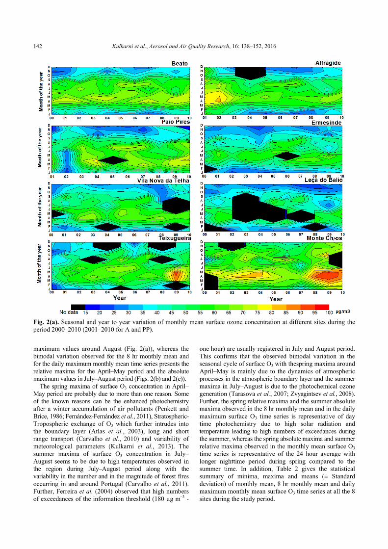
Fig. 2(c). Seasonal and year to year variation of daily maximum monthly mean surface ozone concentration at different sites during the period 2000–2010 (2001–2010 for A and PP).

Table 2. Minimum, Maximum and Mean surface ozone concentration of monthly mean, 8 hr monthly mean and daily maximum monthly mean values at each site.

Site code MM 8 hr MM MM Daily Max

Min Max Mean (± sd) Min Max Mean (± sd) Min Max Mean (± sd)B 22.4 75.0 51.3 (± 14) 30.2 97.2 65.1 (± 15) 41.0 117.6 79.5 (± 17)A 18.7 80.8 50.6 (± 14) 26.4 100.9 63.5 (± 17) 41.3 117.8 79.4 (± 17)PP 17.7 77.6 49.2 (± 15) 22.2 102.6 65.2 (± 20) 31.9 126.7 79.5 (± 22)E 19.2 66.6 42.1 (± 11) 25.8 95.2 59.8 (± 17) 39.7 119.4 59.8 (± 17)

VNT 22.1 69.6 45.4 (± 12) 29.8 92.9 62.5 (± 16) 39.7 111.9 76.8 (± 16)LB 20.6 60.7 39.7 (± 10) 27.2 96.7 57.0 (± 15) 42.2 117.7 71.5 (± 15)T 18.3 94.1 49.3 (± 13) 29.1 110.0 71.4 (± 19) 41.2 134.0 86.6 (± 19)

MC 23.4 95.5 62.7 (± 12) 28.6 103.5 70.1 (± 13) 38.9 115.4 81.8 (± 14)

pollution transport from Porto and Lisbon metropolitans sites to Teixugueira and to Monte Chãos, respectively. This may lead to the transport of O3 produced and O3 precursors released over Lisbon and Porto metropolitan areas (traffic as well as industrial), respectively to Teixugueira and to Monte Chãos monitoring sites, resulting in higher values of surface O3.

Long Term Trend in Surface Ozone Concentration In this sub-section long-term surface O3 trend are analyzed

for both surface O3 time series and deseasonalized surface O3 time series of monthly mean, 8 hr monthly mean and daily maximum monthly mean values at all the 8 sites used in this study. In order to obtain deseasonalized surface O3 time series the major component of natural surface O3 variations


(seasonal component) must be subtracted from each of the three surface O3 time series (Supporting Information SI1-Figs. 1(a), 1(b), 1(c)). The surface O3 time series (Supporting Information SI1-Figs. 1(a), 1(b), 1(c)) and the deseasonalized surface O3 time series (Figs. 3(a), 3(b), 3(c)), respectively of monthly mean, 8 hr monthly mean and daily maximum monthly mean surface O3 concentrations were used to compute linear trends over study locations (all 8 sites) as was explained in Section 2.

Tables 3–5 present the results of both the trend analysis for monthly mean, 8 hr monthly mean and daily maximum monthly mean surface O3 time series and of the deseasonalized

surface O3 time series for the whole period of each station, listing the Mann-Kendall test statistic ‘S’, variance of S ‘V’, significance level ‘Z’ at 90% level of confidence (Z0.05 = 1.68), magnitude of Trend ‘T’ (µg m–3 year–1) and the Trend significance ‘TS’. All the three regions, except two sites i.e., Alfragide and Leça do Balio, show an increasing trend in the monthly mean and daily maximum monthly mean surface O3 time series, and all regions, except one site i.e., Alfragide, show an increasing trend in the 8 hr monthly mean surface O3 time series. However, at most of the sites, except for Alfragide, Teixugueira and Monte Chão sites, the trends are statistically not significant for the

Fig. 3(a). Deseasonalized time series of monthly mean surface ozone concentration at different sites during the period 2000–2010 (2001–2010 for A and PP). Straight lines show the linear fits on the monthly mean surface ozone concentration.


Fig. 3(b). Deseasonalized time series of 8 hr monthly mean surface ozone concentration at different sites during the period 2000–2010 (2001–2010 for A and PP). Straight lines show the linear fits on the 8 hr monthly mean surface ozone concentration.

monthly mean surface O3 time series. Similarly, at all of the sites and except for Alfragide, the trends are statistically not significant for the 8 hr monthly mean and for the daily maximum monthly mean surface O3 time series. Therefore, for further trend analysis, deseasonalized monthly mean, 8 hr monthly mean and daily maximum monthly mean surface O3 time series are used.

In Lisbon region, Beato (B) and Paio Pires (PP) sites show an increasing trend in deseasonalized monthly mean surface O3 time series with high positive Mann-Kendall statistic S (T = 0.44 µg m–3 year–1 and S = 1566) and (T = 1.25 µg m–3

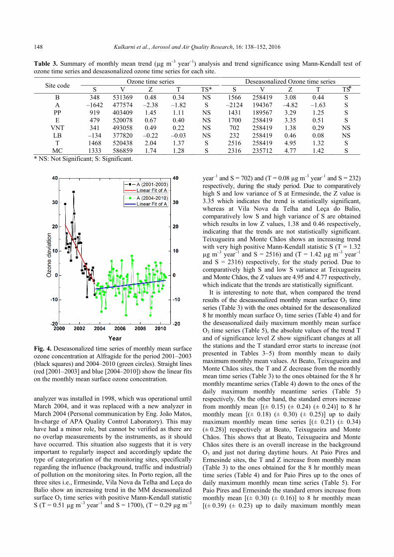
year–1 and S = 1431) respectively, and Alfragide (A) shows a decreasing trend in deseasonalized monthly mean surface O3 time series with high negative Mann-Kendall statistic S (T = –1.63 µg m–3 year–1 and S = –2124) for the study period. All the three sites (B, PP, A) in Lisbon region shows comparatively low S variance which results in a high Z value (Table 3) indicating that the trends are statistically significant. Further analysis of negative trend at Alfragide during the study period reveals that there are in fact two different trend regimes for all the three deseasonalized surface O3 time series, as shown in Fig. 4 (only for deseasonalized


Fig. 3(c). Deseasonalized time series of daily maximum monthly mean surface ozone concentration at different sites during the period 2000–2010 (2001–2010 for A and PP). Straight lines show the linear fits on the daily maximum monthly mean surface ozone concentration.

monthly mean surface O3 time series). The first regime shows a very strong negative trend during the period 2001–2003 and the second regime shows slightly positive trend during the period 2004–2010. The overall negative trend for the entire study period at Alfragide is due to the influence of strong negative trend observed for the period 2001–2003 masking the marginal positive trend observed for the period 2004–2010. This change of the trend regime may be due to two reasons. The first and the main one may be the large scale land-use changes occurred around Alfragide monitoring site in the period (around) 2001–2003 (Kulkarni

et al., 2013) for the construction of the highway ‘CRIL’ (Circular Regional Interior de Lisboa). This may have resulted in the increased emission of NOX from vehicular exhausts, affecting O3 mixing ratios due to titration effect of local high NOx emissions. By analyzing the NO and NO2 time series (NOx = NO + NO2) two different regimes can be observed (Supporting Information SI3-Figs. 3(a) and 3(b)) in the periods (a) 2001–2003 and (b) 2004–2010, as in the case of surface O3 at the Alfragide site (Fig. 4). The second reason may be due to the change of the surface O3 analyzer at the Alfragide site. The first surface O3


Table 3. Summary of monthly mean trend (µg m–3 year–1) analysis and trend significance using Mann-Kendall test of ozone time series and deseasonalized ozone time series for each site.

Site code Ozone time series Deseasonalized Ozone time series

S V Z T TS* S V Z T TS⃰ B 348 531369 0.48 0.34 NS 1566 258419 3.08 0.44 S A –1642 477574 –2.38 –1.82 S –2124 194367 –4.82 –1.63 S PP 919 403409 1.45 1.11 NS 1431 189567 3.29 1.25 S E 479 520078 0.67 0.40 NS 1700 258419 3.35 0.51 S

VNT 341 493058 0.49 0.22 NS 702 258419 1.38 0.29 NS LB –134 377820 –0.22 –0.03 NS 232 258419 0.46 0.08 NS T 1468 520438 2.04 1.37 S 2516 258419 4.95 1.32 S

MC 1333 586859 1.74 1.28 S 2316 235712 4.77 1.42 S * NS: Not Significant; S: Significant.

Fig. 4. Deseasonalized time series of monthly mean surface ozone concentration at Alfragide for the period 2001–2003 (black squares) and 2004–2010 (green circles). Straight lines (red [2001–2003] and blue [2004–2010]) show the linear fits on the monthly mean surface ozone concentration.

analyzer was installed in 1998, which was operational until March 2004, and it was replaced with a new analyzer in March 2004 (Personal communication by Eng. João Matos, In-charge of APA Quality Control Laboratory). This may have had a minor role, but cannot be verified as there are no overlap measurements by the instruments, as it should have occurred. This situation also suggests that it is very important to regularly inspect and accordingly update the type of categorization of the monitoring sites, specifically regarding the influence (background, traffic and industrial) of pollution on the monitoring sites. In Porto region, all the three sites i.e., Ermesinde, Vila Nova da Telha and Leça do Balio show an increasing trend in the MM deseasonalized surface O3 time series with positive Mann-Kendall statistic S (T = 0.51 µg m–3 year–1 and S = 1700), (T = 0.29 µg m–3

year–1 and S = 702) and (T = 0.08 µg m–3 year–1 and S = 232) respectively, during the study period. Due to comparatively high S and low variance of S at Ermesinde, the Z value is 3.35 which indicates the trend is statistically significant, whereas at Vila Nova da Telha and Leça do Balio, comparatively low S and high variance of S are obtained which results in low Z values, 1.38 and 0.46 respectively, indicating that the trends are not statistically significant. Teixugueira and Monte Chãos shows an increasing trend with very high positive Mann-Kendall statistic S (T = 1.32 µg m–3 year–1 and S = 2516) and (T = 1.42 µg m–3 year–1 and S = 2316) respectively, for the study period. Due to comparatively high S and low S variance at Teixugueira and Monte Chãos, the Z values are 4.95 and 4.77 respectively, which indicate that the trends are statistically significant.

It is interesting to note that, when compared the trend results of the deseasonalized monthly mean surface O3 time series (Table 3) with the ones obtained for the deseasonalized 8 hr monthly mean surface O3 time series (Table 4) and for the deseasonalized daily maximum monthly mean surface O3 time series (Table 5), the absolute values of the trend T and of significance level Z show significant changes at all the stations and the T standard error starts to increase (not presented in Tables 3–5) from monthly mean to daily maximum monthly mean values. At Beato, Teixugueira and Monte Chãos sites, the T and Z decrease from the monthly mean time series (Table 3) to the ones obtained for the 8 hr monthly meantime series (Table 4) down to the ones of the daily maximum monthly meantime series (Table 5) respectively. On the other hand, the standard errors increase from monthly mean [(± 0.15) (± 0.24) (± 0.24)] to 8 hr monthly mean [(± 0.18) (± 0.30) (± 0.25)] up to daily maximum monthly mean time series [(± 0.21) (± 0.34) (± 0.28)] respectively at Beato, Teixugueira and Monte Chãos. This shows that at Beato, Teixugueira and Monte Chãos sites there is an overall increase in the background O3 and just not during daytime hours. At Paio Pires and Ermesinde sites, the T and Z increase from monthly mean (Table 3) to the ones obtained for the 8 hr monthly mean time series (Table 4) and for Paio Pires up to the ones of daily maximum monthly mean time series (Table 5). For Paio Pires and Ermesinde the standard errors increase from monthly mean [(± 0.30) (± 0.16)] to 8 hr monthly mean [(± 0.39) (± 0.23) up to daily maximum monthly mean


Table 4. Summary of 8 hr monthly mean trend (µg m–3 year–1) analysis and trend significance using Mann-Kendall test of ozone time series and deseasonalized ozone time series for each site.


S V Z T TS* S V Z T TS⃰ B 144 536980 0.20 0.23 NS 892 258491 1.76 0.33 S A –1254 417895 –1.94 –1.60 S –1954 194367 –4.43 –1.40 S PP 765 408864 1.20 1.28 NS 1197 189567 2.75 1.43 S E 761 522995 1.05 0.74 NS 1978 258419 3.89 0.86 S

VNT 217 511477 0.30 0.22 NS 786 258419 1.55 0.35 NS LB 48 383535 0.08 0.12 NS 666 258419 1.31 0.25 NS T 1056 533819 1.44 1.32 NS 1904 258419 3.75 1.21 S

MC 1155 542616 1.57 1.14 NS 2214 235712 4.56 1.34 S * NS: Not Significant; S: Significant.

Table 5. Summary of monthly mean daily maximum trend (µg m–3 year–1) analysis and trend significance using Mann-Kendall test of ozone time series and deseasonalized ozone time series for each site.


S V Z T TS* S V Z T TS⃰ B 54 534192 0.08 0.12 NS 582 258419 1.15 0.21 NS A –1410 423447 –2.17 –1.85 S –2096 194367 –4.76 –1.68 S PP 755 417990 1.17 1.42 NS 1029 189567 2.37 1.55 S E 623 521828 0.86 0.57 NS 1662 258417 3.27 0.66 S

VNT 162 511614 0.23 0.10 NS 571 258418 1.13 0.23 NS LB –99 387622 –0.16 –0.09 NS 346 258419 0.68 0.02 NS T 1065 544951 1.44 1.19 NS 1556 258417 3.06 1.07 S

MC 822 533629 1.13 0.84 NS 1670 235712 3.44 1.05 S * NS: Not Significant; S: Significant.

[(± 0.46) (± 0.27)] respectively. This shows that at Paio Pires and Ermesinde, there is a higher increase of surface O3

during daytime hours than the background O3. At Alfragide the magnitudes of T and Z increase from the ones obtained for the monthly meantime series up to the ones obtained for the 8 hr monthly mean series but decrease from the ones obtained for the monthly mean to the ones obtained for the daily maximum monthly mean time series whereas the standard errors decrease from monthly mean (± 0.24) down to 8 hr monthly mean (± 0.23) and increases from MM to daily maximum monthly mean (± 0.28). The trend T at Vila Nova da Telha and Leça do Balio are not statistically significant for all the three deseasonalized surface O3 time series, so the change in T, Z and T standard error will not give clear conclusions.

It can be noted that PP, T and MC sites show higher T for monthly mean (Table 3), 8 hr monthly mean (Table 4) and daily maximum monthly mean (Table 5) surface O3 time series and forthe deseasonalized surface O3 time series compared to other 5 sites. As described in previous sub-section and from Fig. 1, it is clear that Teixugueira, Paio Pires and Monte Chãos are located downwind of Porto and Lisbon metropolitan areas. Generally, sites located downwind regions of big metropolitan areas shows higher trend T due to regional impact and transport of O3 and O3 precursors (von Schneidemesser et al., 2014).

The European policy review (ACCENT) has concluded that there is strong evidence that background O3 concentrations in the northern hemisphere have increased by

up to 10 µg m–3 per decade over the last 20–30 years (Raes and Hjorth, 2006). The trends revealed by O3 soundings for the middle and upper troposphere (Logan, 1999) broadly agree with those from the surface observations. Furthermore tropospheric O3 values were compared over the Iberian Peninsula for the two periods (1979–1993 and 1997–2005) and a systematic increase in the number of months with higher tropospheric O3 concentration has been observed during the second period with respect to the first suggesting increase in Tropospheric O3 in the last decade (Kulkarni et al., 2011b).The increasing trend of background surface O3 and of free tropospheric O3 observed by various researchers (Logan, 1999; Raes and Hjorth, 2006; Kulkarni et al., 2011b) are considered to be driven by increasing emissions of man-made tropospheric O3 precursor gases, particularly methane, VOCs, CO and NOx since pre-industrial times. Lifetime of surface O3 is short (few hours to couple of days, depending on the location and time of observation) compared to aloft or free tropospheric O3 (IPCC, 2001). The increasing trend of free tropospheric O3 and of the background surface O3 may be one of the reasons for positive trendsalso observed over Portugal, at the different sites analyzed in this study, all classified as background sites, independently of their type of environment being urban or suburban. CONCLUSIONS

The seasonal variation of surface O3 concentration in Portugal was characterized by bimodal variation in the


annual cycle with spring and summer maxima, with a slight dip around June, and the winter minima. In the bimodal variation observed in themonthly mean surface O3 time series, the absolute maxima occurs in the spring season and the relative maxima in the summer, while in the bimodal variation observed in the 8 hr monthly mean and in the daily maximum monthly mean surface O3 time series, the relative maxima occurs in the spring and the absolute maxima in the summer. The observed change in the occurrence of absolute and relative maxima during the spring and summer in the monthly mean surface O3 time series compared to 8 hr monthly mean and the daily maximum monthly mean surface O3 time series can be attributed to:

1. The day time photochemistry, due to high solar radiation and temperature, is more intense during the summer than during the spring, leading to high numbers of exceedances and to the occurrence of absolute maxima in the summer in both the 8 hr and the daily maximum monthly mean surface O3 time series.

2. The monthly mean surface O3 time series is representative of 24 hour average of days with longer nighttime period during spring compared to the summer time.

All stations show large inter-annual variation in the surface O3 concentration averaged over the study period, varying from 40 up to 62 (± 10–15) µg m–3 for monthly mean surface O3 time series, from 57 up to 71 (± 13–20) µg m–3

for 8 hr monthly mean surface O3 time series and from 60 up to 87 (± 14–22) µg m–3 for the daily maximum monthly mean surface O3 time series. Suburban sites located away but downwind from Lisbon and Porto metropolitan areas, such as Teixugueira and Monte Chão, showed higher 8 hr monthly mean and daily maximum monthly mean surface O3 concentrations, averaged over the study period, than sites (urban/suburban) located inside the two metropolitan areas.

A trend analysis showed that in general the annual cycle (summer maxima and winter minima) of surface O3

concentration masks the actual trend values, sometimes even polarity, and their statistical significance due to low Mann-Kendall test statistic ‘S’ and high variance of S ‘V’. This implies that the deseasonalization of original surface O3 time series is very important before calculating trends. An increasing long term trend in the deseasonalized monthly mean, 8 hr monthly mean and daily maximum monthly mean time series of surface O3 was observed at 7 out of 8 stations located inthe different parts of Portugal used in this study. Out of 8 stations, 6 stations (5 positive and 1 negative) show statistically significant trends in the monthly mean and 8 hr monthly mean surface O3 time series, whereas 5 stations (4 positive and 1 negative) show statistically significant trend in the daily maximum monthly mean surface O3 time series with high Z values. Further the suburban sites (PP, T and MC) located downwind region of big metropolitan areas (Lisbon and Porto) show higher trend values due to transport of O3 and O3 precursors. The two different trend regimes observed at Alfragide shows the effect of land-use changes and the influence of development activities on the monitoring sites and warrants regular inspection and updating of the classification of the measuring station, specifically regarding the influence (background, traffic and industrial)

of pollution on the monitoring sites. ACKNOWLEDGEMENT

Author (PSK) is thankful to Fundaçãopara a Ciência e a Tecnologia (FCT) for the grant SFRH/BPD/82033/2011. Thanks are also due to Agência Portuguesa do Ambiente (APA) (http://www.qualar.apambiente.pt/) for surface ozone data. We also thank Eng. João Matos, In-charge of APA Quality Control Laboratory. The paper was partially funded through FEDER (Programa Operacional Factores de Competitividade-COMPETE) and National funding through FCT-Fundaçãopara a Ciência e a Tecnologia in the framework of project FCOMP-01-0124-FEDER-014024 (Refª. FCT PTDC/AAC-CLI/114031/2009).The authors acknowledge the funding provided by ICT, under contract with FCT (the Portuguese Science and Technology Foundation). SUPPLEMENTARY MATERIALS

Supplementary data associated with this article can be found in the online version at http://www.aaqr.org. REFERENCES Alvim-Ferraz, M.C.M., Sousa, S.I.V., Pereira, M.C. and

Martins, F.G. (2006). Contribution of Anthropogenic Pollutants to the Increase of Tropospheric Ozone Levels in the Oporto Metropolitan Area, Portugal since the 19th Century. Environ. Pollut. 140: 516–524.

AQEG (2009). Air Quality Expert Group-Ozone in the United Kingdom: Chapter 2. Temporal Trends and Spatial Distributions in Ozone Concentrations Determined from Monitoring Data. Department for the Environment, Food and Rural Affairs. AQEG Report 5: 15–62.

Atlas, E.L., Ridley, B.A. and Cantrell, C.A. (2003). The Tropospheric Ozone Production about the Spring Equinox (TOPSE) Experiment: Introduction. J. Geophys. Res. 108: 8353.

Brönnimann, S., Buchmann, B. and Wanner, H. (2002). Trends in Near-Surface Ozone Concentrations in Switzerland: The 1990s. Atmos. Environ. 36: 2841–2852.

Carslaw, D.C. (2005). On the Changing Seasonal Cycles and Trends of Ozone at Mace Head, Ireland. Atmos. Chem. Phys. 5: 3441–3450.

Carvalho, A., Monteiro, A., Ribeiro, I., Tchepel, O., Miranda, A.I., Borrego, C., Saavedra, S., Souto, J.A. and Casares, J.J. (2010). High Ozone Levels in the Northeast of Portugal: Analysis and Characterization. Atmos. Environ. 44: 1020–1031.

Carvalho, A., Monteiro, A., Flannigan, M., Solman, S., Miranda, A.I. and Borrego, C. (2011). Forest Fires in a Changing Climate and Their Impacts on Air Quality. Atmos. Environ. 45: 5545–5553.

Censes (2011). http://www.ine.pt/scripts/flex_v10/Main.html De Leeuw, F. (2000). Trends in Ground Level Ozone

Concentrations in the European Union. Environ. Sci. Policy 3: 189–199.


DIRECTIVE 2008/50/Ec of the European Parliament and of The Council (2008) of 21 May 2008 on Ambient Air Quality and Cleaner Air for Europe, Official Journal of the European Union 152: 1–44.

European Commission, DG-REGIO (2006). Study on Strategic Evaluation on Transport Investment Priorities under Structural and Cohesion Funds for the Programming Period 2007–2013. No. 2005.CE.16.0.AT. 014, 2006. Country Report Portugal. http://ec.europa.eu/regional _policy/sources/docgener/evaluation/pdf/evasltrat_tran/portugal.pdf.

Felzer, B.S., Cronin, T., Reilly, J.M., Melillo, J.M. and Wang, X. (2007). Impacts of Ozone on Trees and Crops. C.R. Geosci. 339: 784–798.

Ferreira, F.C., Torres, P.M., Tente, H.S., Jorge, B. and Neto, J.B. (2004). Ozone Levels in Portugal: the Lisbon Region Assessment. Em Proceedings of Air and Waste Management’s 97th Annual Conference and Exhibition. June 22–25, 2004.

Ghude, S.D., Beig, G., Kulkarni, P.S., Kanawade, V.P., Fadnavis, S. and Remedios, J.J. (2011a). Regional CO Pollution over the Indian-Subcontinent and Various Transport Pathways as Observed by MOPITT. Int. J. Remote Sens. 32: 6133–6148.

Ghude, S.D., Kulkarni, S.H., Kulkarni, P.S., Kanawade, V.P., Fadnavis, S., Pokhrel, S., Jena, C., Beig, G. and Bortoli, D. (2011b). Anomalous low Tropospheric Column Ozone over Eastern India during 2002 Severe Drought Event: A Case Study. Environ. Sci. Pollut. Res. 18: 1–14.

Hogrefe, C., Rao, S.T., Zurbenko, L.G. and Porter, P.S. (2000). Interpreting the Information in Ozone Observations and Model Predictions Relevant to Regulatory Policies in Eastern United Station. Bull. Am. Meteorol. Soc. 81: 2083–2106.

Husar, R.B. (1996). Pattern of 8-Hour Daily Maximum O3 and Comparison with the 1-Hour Standard, 1996. http://capital.wustl.edu/otag/reports/8HDMAXO3/Dmax8hr.html.

IPCC Climate change (2001). The Scientific Basis. Intergovernmental Panel on Climate Change. Cambridge University Press, Cambridge, UK. http://www.ipcc.ch/ ipccreports/tar/wg1/index.htm.

Jain, S.L., Arya, B.C., Kumar, A., Ghude, S.D. and Kulkarni, P.S. (2005). Observational Study of Surface Ozone at New Delhi, India. Int. J. Remote Sens. 26: 3515–3526.

Khambhammettu, P. (2005). Mann-Kendall Analysis. Annual Groundwater Monitoring Report of Hydro Geologic Inc., Fort Ord, California.

Kulkarni, P.S., Jain, S.L., Ghude, S.D., Arya, B.C., Dubey, P.K. and Shahnawaz (2009). On Some Aspects of Tropospheric Ozone Variability over the Indo-Gangetic (IG) Basin, India. Int. J. Remote Sens. 30: 4111–4122.

Kulkarni, P.S., Ghude, S.D. and Bortoli, D. (2010). Tropospheric Ozone (TOR) Trend over Three Major Inland Indian Cities: Delhi, Hyderabad and Bangalore. Ann. Geophys. 28: 1879–1885.

Kulkarni, P.S., Ghude, S.D., Jain, S.L., Arya, B.C., Dubey,

P.K. and Shahnawaz (2011a). Tropospheric Ozone Variability over the Indian Coastline and Adjacent Land and Sea. Int. J. Remote Sens. 32: 1545–1559.

Kulkarni, P.S., Bortoli, D., Salgado, R., Antón, M., Costa, M.J. and Silva, A.M. (2011b). Tropospheric Ozone Variability over the Iberian Peninsula. Atmos. Environ. 45: 174–182.

Kulkarni, P.S., Bortoli, D. and Silva, A.M. (2013). Nocturnal Surface Ozone Enhancement and Trend over Urban and Suburban Sites in Portugal. Atmos. Environ. 71: 251–259.

Lefohn, A.S., Shadwick, D.S. and Ziman, S.D. (1998).The Difficult Challenge of Attaining EPA’s New Ozone Standard. Environ. Sci. Technol. 32: 276–282.

Logan, J.A. (1999). An Analysis of Ozone Sonde Data for the Troposphere: Recommendations for Testing 3-D Models and Development of a Gridded Climatology for Tropospheric Ozone. J. Geophys. Res. 104: 16115–16150.

Fernández-Fernández, M.I., Gallego, M.C., García, J.A. and Acero, F.J. (2011). A Study of Surface Ozone Variability over the Iberian Peninsula during the Last Fifty Years. Atmos. Environ. 45: 1946–1959.

Madureira, H., Andresen, T. and Monteiro, A. (2011). Green Structure and Planning Evolution in Porto. Urban For. Urban Greening 10: 141–149.

McBean, E. and Motiee, H. (2008). Assessment of Impact of Climate Change on Water Resources: A Long Term Analysis of the Great Lakes of North America. Hydrol. Earth Syst. Sci. 12: 239–255.

Mickley, L.J., Murti, P.P., Jacob, D.J., Logan, J.A., Koch, D.M. and Rind, D. (2001). Radiative Forcing from Tropospheric Ozone Calculated with a Unified Chemistry-Climate Model. J. Geophys. Res. 104: 30153–30172.

Monteiro, A., Carvalho, A., Ribeiro, I., Scotto, M., Barbosa, S., Alonso, A., Baldasano, J.M., Pay, M.T., Miranda, A.I. and Borrego, C. (2012). Trends in Ozone Concentrations in the Iberian Peninsula by Quantile Regression and Clustering. Atmos. Environ. 56: 184–193.

Monteiro, A., Lopes, M., Miranda, A.I., Borrego, C. and Vautard, R. (2005). Air Pollution Forecast in Portugal: A Demand from the New Air Quality Framework Directive. Int. J. Environ. Pollut. 25: 4–15.

Olofintoye, O.O. and Sule, B.F. (2010). Impact of Global Warming on the Rainfall and Temperature in the Niger Delta of Nigeria. USEP: Journal of Research Information in Civil Engineering 7: 33–48.

Penkett, S.A. and Brice, K.A. (1986). The Spring Maximum in Photo-Oxidants in the Northern Hemisphere Troposphere. Nature 319: 655–658.

Pereira, M.C., Alvim-Ferraz, M.C.M. and Santos, R.C. (2005). Relevant Aspects of Air Quality in Oporto (Portugal): PM10 and O3. Environ. Monit. Assess. 101: 203–221.

Pio, C.A., Feliciano, M.S., Vermeulen, A.T. and Sousa, E.C. (2002). Seasonal Variability of Ozone Dry Deposition under Southern European Climate Conditions, in Portugal. Atmos. Environ. 34: 195–205.

Premuda, M., Petritoli, A., Masieri, S., Palazzi, E., Kostadinov, I., Bortoli, D., Ravegnani, F. and Giovanelli,


G. (2013). A Study of O3 and NO2 Vertical Structure in a Coastal Wooded Zone near a Metropolitan Area, by Means of DOAS Measurements. Atmos. Environ. 71: 104–114.

Qin, Y., Tonnesen, G.S. and Wang, Z. (2004). One-Hour and Eight-Hour Average Ozone in the California South Coast Air Quality Management District: Trends in Peak Values and Sensitivity to Precursors. Atmos. Environ. 38: 2197–2207.

Raes, F. and Hjorth, J. (2006). Answers to the Urbino Question. ACCENT Secretariat, Universita di Urbino, Italy, ISBN 92-79-02413-2.

Saito, S., Nagao, I. and Tanaka, H. (2002). Relationship of NOx and NMHC to Photochemical O3 Production in a Coastal and Metropolitan Areas of Japan. Atmos. Environ. 36: 1277–1286.

Sather, M.E., Varns, J.L., Mukik, J.D., Glen, G., Smith, L. and Stallings, C. (2001). Passive Ozone Network of Dallas: a Modeling Opportunity with Community Involvement. Environ. Sci. Technol. 35: 4426–4435.

Sicard, P., Coddeville, P. and Galloo, J.C. (2009). Near-Surface Ozone Levels and Trends at Rural Stations in France over the 1995–2003 Period. Environ. Monit. Assess. 156: 141–157.

Sousa, S.I.V., Pereira, M.M.C., Martins, F.G. and Alvim-Ferraz, M.C.M. (2008). Identification of Regions with High Ozone Concentrations Aiming the Impact Assessment on Childhood Asthma. Human and Ecological Risk Assessment. Hum. Ecol. Risk Assess. 14: 610–622.

Sousa, S.I.V., Pires, J.C.M., Martins, F.G., Pereira, M.C. and Alvim-Ferraz, M.C.M. (2009a). Potentialities of Quantile Regression to Predict Ozone Concentrations. Environmetrics 20: 147–158.

Sousa, S.I.V., Alvim-Ferraz, M.C.M., Martins, F.G. and Pereira, M.C. (2009b). Ozone Exposure and Its Influence on the Worsening of Childhood Asthma. Allergy 64: 1046–1055.

Sousa, S.I.V., Martins, F.G., Pereira, M.M.C., Alvim-Ferraz, M.C.M., Ribeiro, H., Oliveira, M. and Abreu, I. (2010).Use of Multiple Linear Regressions to Evaluate

the Influence of O3 and PM10 on Biological Pollutants. Int. J. Civil Eng. Environ. Eng. 2: 107–112.

Tarasova, O.A., Brenninkmeijer, C.A.M., Jöckel, P., Zvyagintsev, A.M. and Kuznetsov, G.I. (2007). A Climatology of Surface Ozone in the Extra Tropics: Cluster Analysis of Observations and Model Results. Atmos. Chem. Phys. 7: 6099–6117.

Unger, N., Shindell, D.T., Koch, D.M. and Streets, D.G. (2006). Cross Influences of Ozone and Sulfate Precursor Emissions Changes on Air Quality and Climate. PNAS 103: 4377–4380.

USEPA (1996). Air Quality Criteria for O3 and Related Photochemical Oxidants. EPA/600/P-93/004a-cF, 1996.

Velasco, P., Popejoy, D. and Panson, A. (2000). Recommended Area Designations for Federal Eight-Hour O3 Standard. http://www.arb.ca.gov/desig/8-houro z/staffr pt.pdf.

Von Schneidemesser, E., Vieno, M. and Monks, P.S. (2014). The Changing Oxidizing Environment in London-Trends in Ozone Precursors and Their Contribution to Ozone Production. Atmos. Chem. Phys. Discuss. 14: 1287–1316, doi: 10.5194/acpd-14-1287-2014, 2014.

West, J.J., Fiore, A.M., Horowitz, L.W. and Mauzerall, D.L. (2006). Global Health Benefits of Mitigating Ozone Pollution with Methane Emission Controls. PNAS 103: 3988–3993.

Zhang, R., Lei, W., Tie, X. and Hess, P. (2004). Industrial Emissions Cause Extreme Urban Ozone Diurnal Variability. PNAS 101: 6346–6350.

Zvyagintsev, A.M., Kakadzhanova, G., Kruchenitskii, G.M. and Tarasova, O.A. (2008). Periodic Variability of Surface Ozone Concentration over Western and Central Europe from Observational Data. Russ. Meteorol. Hydrol. 33: 159–166.

Received for review, February 14, 2015 Revised, May 21, 2015

Accepted, June 30, 2015

Documents

Surface Ozone Variability and Trend over Urban and