Embed Size (px)
Citation preview
Correction: 19 October 2006
www.sciencemag.org/cgi/content/full/312/5782/1959/DC1
Supporting Online Material for
Rapid Advance of Spring Arrival Dates in Long-Distance Migratory Birds
Niclas Jonzén, Andreas Lindén, Torbjørn Ergon, Endre Knudsen, Jon Olav Vik, Diego Rubolini, Dario Piacentini, Christian Brinch, Fernando Spina, Lennart Karlsson,
Martin Stervander, Arne Andersson, Jonas Waldenström, Aleksi Lehikoinen, Erik Edvardsen, Rune Solvang, Nils Chr. Stenseth*
*To whom correspondence should be addressed. E-mail: [email protected]
Published 30 June 2006, Science 312, 1959 (2006)
DOI: 10.1126/science.1126119
This PDF file includes:
Materials and Methods SOM Text Tables S1 to S5 References
Correction (19 October 2006): On page 6, there are a few typographical errors in the equations in the middle paragraph. The paragraph should read as follows: A Gaussian (normal) seasonal distribution curve can be fitted as a quadratic function on a logarithmic scale (log({expected number on day xi}) 2
210 iii xx βββµ ++== )). However, the following re-parameterization gave lower autocorrelations in the MCMC simulations: “mean” ( )21 2/ ββτ −== , “peak” 2
210 τβτββρ ++== , and “standard
deviation” 22/1 βκ −== .

Supporting Online Material
Data
We analyzed banding data collected during spring migration in the period 1980–2004 at the
bird observatories of Falsterbo (Sweden), Ottenby (Sweden), Jomfruland (Norway) and
Hanko (Finland) (Fig. 1). For Hanko and Jomfruland, we also included observations from
standardized counts of migrants (see below). A total of 34 species were investigated (Tables
S1–S3; see below for selection criteria), of which 17 were classified as short-distance
(wintering north of the Sahara desert, mainly in Europe) and 17 as long-distance migrants
(wintering south of the Sahara or in South Asia). For trapping and observation data, care was
taken not to include any species for which local wintering or breeding birds potentially could
influence our sample percentiles.
For comparison with southern Europe, we used banding data based on standardized
mist-netting from the island of Capri (southern Italy). Below we summarize details of the data
collection procedures at each observatory.
Jomfruland
Jomfruland Bird Observatory (S1) is located close to the northern end of the island of
Jomfruland, along the outer coastline of southeastern Norway (58°53'N, 9°37'E). We used
data on birds trapped in mist-nets during the period April 1–June 15. For some common
species with low trapping efficiency or an early migration (i.e. where migrating birds may
occur prior to the start of the mist-netting period), we instead used daily observation sums for
the period March 18–June 15. From 1990 onwards, the mist-netting protocol has remained
unchanged, with the number, positions, and operating hours of mist-nets kept constant.
Trapping was performed daily, but the number of nets and/or their hours of operation were
1

reduced on days with strong wind and/or heavy rain. Prior to 1990, sampling efforts were less
strictly standardized, but trapping occurred on a daily basis throughout the selected period.
For these early years, care was taken to use only data from the same trapping location as later
years, and we did not include any observation data for years with incomplete coverage before
the onset of mist-netting.
Falsterbo
The banding site at the Falsterbo Bird Observatory is situated on the south-westernmost tip of
Sweden (55°23'N, 12°50'E). Standardized mist-netting in spring is performed daily at the
Lighthouse Garden, a small (ca. 1 ha) stand of mixed trees and bushes surrounding the
Falsterbo Lighthouse (S2), within an open field area (golf course). Since 1980, the spring
trapping season started on March 21 and lasted till June 10. Depending on weather conditions
(wind in particular), the daily number of mist-nets used varied, up to a maximum of 21. On
days with heavy rain or very strong winds, all trapping efforts were canceled. The nets were
opened before dawn and controlled every half hour. The daily trapping period lasted at least
four hours and continued thereafter as long as the number of captured birds exceeded ten
individuals per hour. Nets have been positioned at the same location during all years.
Ottenby
Ottenby Bird Observatory (56°12'N, 16°24'E) is situated on the southernmost tip of Öland, a
137 km long island, ca.10 km off the coast of south-eastern Sweden. Migratory birds have
been caught according to strictly standardized procedures during 1980–2004 (S3). Birds were
caught in stationary mist nets and in two funnel traps of Helgoland type (S4), every morning
from dawn to 11 am. In case of rain or strong winds only the funnel traps were used. The
2
spring trapping period was March 15–June 15, and only 14 out of 2,325 trapping days had to
be cancelled over the years (all comprised between 15–24 March in the years 1980–1987).
Hanko
Hanko bird observatory (59°48'N, 22°53'E) is located on a peninsula in the south-western part
of Finland (S5). Data were collected by means of two daily routines: standardized counts of
actively migrating birds and counts of resting migratory passerines. For further analysis, we
used either one of the methods or the sum of both, depending on the species-specific breeding
status in the area, the migratory behavior and commonness in the respective set of data. We
used data from the period March 10 to June 15. To avoid bias due to non-randomly missing
days early in the season, we excluded some early-migrating short-distance migrants from the
analyses (see Tables S1–S3). Standardized migration counts consisted of four hours of
continuous observation from sunrise onwards in a tower near the tip of the peninsula. Poor
weather conditions (heavy rain and/or very strong wind) occasionally reduced observation
activity, but during such weather conditions passerine migration is extremely scarce. Resting
migratory passerines were counted along routine walking paths at the small (ca. 12 ha)
observatory area at the tip of the peninsula after the standardized migration counts.
Capri
The island of Capri (40°33'N 14°15'E) is located in the Tyrrhenian sea, ca. 5 km off mainland
southern Italy. During spring, many long-distance migratory birds stop there to rest, mainly
for a short time (often only a few hours), after the consecutive crossing of the Sahara desert
and of the Mediterranean Sea (S6–S9). Birds were trapped with mist-nets, whose location was
kept standardized during the study period (see below), while vegetation structure was affected
during few years by a fire event (S8); however, this should not affect changes in the
3
phenology of migration. The trapping area comprises ca. 2 ha of the dry and bushy vegetation
(garrigue and “macchia”) typical of this region of the Mediterranean. Data were collected
during the period 1981-2004, although no data were available for the years 1982 to 1985, and
for the year 2000, when the coverage was insufficient (S8). Trapping activities were carried
out every day (from dawn to dusk) during the selected time period (see below), except in
cases of heavy wind or rain; this occurred on average 1.05 days each year, with no temporal
trend over the study period (slope = 0.060 ± 0.056 SE). In order to standardize the trapping
effort across years (see S8), the data used in this study was restricted to the period April 17–
May 15. Since the proportions of the birds arriving outside these dates may vary from year to
year, simple percentiles from banding dates may be biased and underestimate the variation in
mean arrival dates. We therefore fitted a Gaussian curve in a Poisson regression on the daily
banding numbers and used the distribution derived from this analysis to estimate percentiles
of the yearly migratory distributions. To be able to account for large extra-Poisson variation
in the data, the model was fitted with Bayesian MCMC methods (see Methods).
Climate data
We used the mean winter (December–March) NAO index
(http://www.cgd.ucar.edu/cas/jhurrell/) as a measure of climate fluctuations, because it is
known to affect the timing of spring events in Europe (S10). As an explanatory variable, we
used the deviations from linear regression of the winter NAO index on year (dNAO). The
trend was weakly negative over this time period (slope = –0.052, 95% c.i.: –0.167 to 0.063).
Methods
For each species and year in which at least 20 individuals were trapped/observed at a
Scandinavian bird observatory, we estimated the 10th, 50th and 90th sample percentiles. Dates
4
are given as Julian dates (day-of-year). Note that the estimated percentiles are not, strictly
speaking, independent, and fitting a Gaussian curve to the Capri data results in a different
statistical dependence between the percentiles.
Models and statistics
We tested whether regression coefficients for short- and long-distance migrants differed
significantly from each other by constructing a 95% confidence interval for the difference
using maximum likelihood and checked whether zero was excluded. To test whether the
regression coefficients differed from zero, we checked whether the bivariate 95% confidence
region of their means (Fig. 2) excluded zero with respect to the TIME or dNAO axis.
For each species and percentile (10th, 50th and 90th) of the arrival distribution (S11)
we fitted a linear mixed-effects model having TIME and the residuals of the regression of
NAO on TIME (dNAO) as explanatory variables, ‘observatory’ as a fixed effect and a random
between-year variance component in common for all observatories. Note that a unit change in
NAO implies an identical change in dNAO, even if the origins of the two scales differ. Thus,
we have framed our discussion simply in terms of effects of a change in NAO. Furthermore,
to facilitate comparison between the observatories and the banding site on Capri, the mean
effects of TIME and dNAO were estimated for the six long-distance migrants for which
sufficient data were available both at the four Scandinavian bird observatories and on Capri
(see “Estimating mean arrival date in the Capri data by over-dispersed Poisson regression”).
Estimates were obtained from a linear mixed model assuming compound symmetry for the
year-to-year variation of different species (i.e., same variance for all species and all species
equally correlated), and a different residual variance for every combination of species and
locations (because the amount of data, and hence measurement error, behind every data point
in the analysis vary mainly at this level). The mixed models were fitted with restricted
5
maximum likelihood (REML) by the ‘lme’ function in the nlme package (S12) of the software
R (version 2.1) (S13).
Estimating mean arrival date in the Capri data by over-dispersed Poisson regression
Because data from the Capri banding site did not cover the entire migration period (see Data),
mean arrival date at this location was estimated by fitting a Gaussian seasonal distribution
curve in a Poisson regression on the daily banding numbers. There is typically large day-to-
day variation in banding data of migrating birds (presumably mostly due to local weather
conditions), and it is difficult to adequately model this over-dispersion in generalized linear
models when using maximum likelihood methods. We therefore used Bayesian MCMC
methods implemented in the program WinBUGS 1.4 (S14).
A Gaussian (normal) seasonal distribution curve can be fitted as a quadratic function
on a logarithmic scale (log({expected number on day xi}) = )).
However, the following re-parameterization gave lower autocorrelations in the MCMC
simulations: “mean”
2210 iii xx βββµ ++=
)2/( 21 ββτ −== , “peak height” 2
21
02
210 4βββτβτββρ −=++== , and
“standard deviation” 22/1 βκ −== .
Two alternative models were considered for modeling the over-dispersion in the data;
either a log-normal component of the Poisson parameter ( iii εµλ +=)log( , where
), or a stochastic day-effect from a Gamma distribution with shape parameter
being 1/scale parameter ( , where
),0(~ 2σε Ni
iiie υλ µ= )/1,(~ ααυ Γi , 1)E( i =υ ). In the first model, the
expected number of ringed birds on day i is . In the latter model, the expected
number is . The Gamma-model gave somewhat better goodness of fit statistics (see
below) and lower DIC (=Deviance Information Criterion) value, and was hence used in the
2/i
2
)E( σµλ += ie
ieµλ =)E( i
6

analysis. The model was fitted for each species separately, and all parameters except α were
year-specific (α was constant across years). As estimates of mean arrival dates (see Table s5)
we used the medians of posterior distributions of the parameterτ .
To facilitate numerical convergence and eliminate nonsensical parameter values from
the posterior distributions, we constrained the parameter space by using uniform and rather
vague priors on the parameters τ (mean passage date) and κ (standard deviation in passage
date). For κ of all years and species, we used a Uniform (0.25,10) prior, meaning that the
time elapsed between the 2.5 percentile and the 97.5 percentile of banding dates could take
any value between 1 and 40 days. The priors for mean banding date,τ , depended on species
and spanned what we considered the maximum reasonable range for that species (Table S4).
The peak of the expectation curve, represented by the parameterρ , was allowed to vary
between 0 and 10 times the maximum observed daily count of the species, which is
essentially an uninformative prior. The prior of the parameter in the Gamma-term accounting
for over-dispersion, α , was set to an uninformative )1000 shape 1/1000, scale( ==Γ
distribution.
We used relatively long chains in the MCMC simulations due to persistent long-
legged autocorrelations in some parameters (6 parallel chains of 80,000 iterations with an
initial burn-in period of 10,000 iterations and thereafter sampling at every 5th iteration).
Convergence was confirmed by the Gelman and Rubin statistic, which compares the within-
chain to the between-chain variability of chains started at different and dispersed initial values
(S15).
Goodness of fit (GOF) was assessed by using Bayesian p-values (comparing the
distributions of GOF-statistics computed from both the actual data and from simulated data at
every step of the MCMC chain (S16). An acceptable fit was verified with respect to the
following statistics: deviance, skewness and kurtosis of deviance residuals, correlation
7
between deviance residuals and day of year (xi), and correlation between the deviance
residuals and the fitted expectations . ieµ
References
S1. E. Edvardsen et al., Bestandsovervåking Ved Standardisert Fangst og Ringmerking ved
Fuglestasjonene (Report no. 3–2004, Norwegian Ornithological Society, Trondheim, 2004).
S2. L. Karlsson, S. Ehnbom, K. Persson, G. Walinder, Ornis Svecica 12, 113 (2002).
S3. M. Stervander, Å. Lindström, N. Jonzén, A. Andersson, J. Avian Biol. 36, 210 (2005).
S4. H. Bub, Bird trapping and bird banding – a handbook for trapping methods all over the
world (Cornell University Press, Hong Kong, 1991).
S5. A. V. Vähätalo, K. Rainio, A. Lehikoinen, E. Lehikoinen, J. Avian Biol. 35, 210 (2004).
S6. A. Pilastro, F. Spina, J. Avian Biol. 28, 309 (1997).
S7. D. Rubolini, F. Spina, N. Saino, Biol. J. Linn. Soc. 85, 199 (2005).
S8. N. Jonzén et al., Ornis Svecica 16, 27 (2006).
S9. F. Spina, D. Piacentini, A. Montemaggiori, Ornis Svecica 16, 20 (2006).
S10. M. C. Forchhammer, E. Post, N. C. Stenseth, J. Anim. Ecol. 71, 1002 (2002).
S11. T.H. Sparks et al., Global Change Biol. 11, 22 (2005).
S12. J. C. Pinheiro, D. M. Bates, Mixed-Effects Models in S and S-PLUS (Springer, New
York, 2000).
S13. R Development Core Team, R: A Language and Environment for Statistical Computing.
(R Foundation for Statistical Computing, Vienna, 2005) (http://www.r-project.org).
S14. D. Spiegelhalter, A. Thomas, N. Best, D. Lunn, WinBUGS User Manual. Version 1.4
(Technical report, Medical Research Council Biostatistics Unit, Cambridge, 2003)
(http://www.mrc-bsu.cam.ac.uk/bugs).
8

S.15. A. Gelman, in Markov chain Monte Carlo in practice, W. R. Gilks, S. Richardson, D. J.
Spiegelhalter, Eds. (Chapman and Hall, London, 1996), pp. 131-143.
S16. A. Gelman, J. B. Carlin, H. S. Stern, D. B. Rubin, Bayesian Data Analysis (Chapman
and Hall, London, 1995).
9

Supplementary Tables Table S1. Species and observatory specific parameter estimates and variance components when analyzing the early phase of migration (10th percentile) using a linear mixed model with ‘observatory’ as a fixed effect and a random between-year variance component in common for all observatories.
Mean date (day of year)* Variance components (SD units)
Estimates of slope (± SE)
Common name Scientific name
Migration category
(SHORT or LONG distance
migrant) Falsterbo Ottenby Jomfru–
land Hanko
Between years
(% of total variance)
Between years within
observatories
TIME (days / year)
dNAO (days / unit)
Estimated unexplained between-year
variation (SD)
White wagtail Motacilla alba SHORT
100.6 107.1 103.0 105.1 3.3 (31 %) 4.9 –0.13 ± 0.15 0.29 ± 0.54 3.3 Winter wren Troglodytes troglodytes SHORT 90.1 89.7 – - 4.0 (52 %) 3.8 –0.09 ± 0.13 –1.10 ± 0.47 3.6 Hedge accentor Prunella modularis SHORT 91.2 89.1 95.8 - 4.4 (57 %) 3.9 –0.05 ± 0.14 –0.68 ± 0.52 4.4 European robin Erithacus rubecula SHORT 95.1 99.7 – - 1.9 (15 %) 4.6 –0.03 ± 0.11 –0.28 ± 0.40 2.1 Common blackbird Turdus merula SHORT 86.5 80.3 – - 1.1 (5 %) 4.5 –0.14 ± 0.09 –0.58 ± 0.32 0.0 Song thrush Turdus philomelos SHORT 91.8 94.9 98.0 101.5 3.2 (31 %) 4.8 –0.12 ± 0.11 –0.47 ± 0.41 3.2 Redwing Turdus iliacus SHORT 97.6 90.8 93.6 4.8 (32 %) 6.9 0.18 ± 0.19 –1.65 ± 0.70 3.9 Chiffchaff Phylloscopus collybita SHORT 101.6 112.5 108.8 114.7 2.3 (17 %) 5.1 –0.26 ± 0.08 –0.21 ± 0.32 1.4 Goldcrest Regulus regulus SHORT 89.7 99.7 90.4 - 2.0 (19 %) 4.2 –0.04 ± 0.09 –0.34 ± 0.34 2.1 Blue tit Parus caeruleus SHORT 83.5 78.7 – - 0.0 (0 %) 2.7 –0.06 ± 0.15 –0.07 ± 0.39 0.0 Great tit Parus major SHORT 82.9 80.1 – - 3.1 (40 %) 3.8 –0.20 ± 0.12 –0.74 ± 0.47 2.7 Chaffinch Fringilla coelebs SHORT 89.4 89.8 – 100.4 3.6 (47 %) 3.9 0.02 ± 0.11 –0.97 ± 0.41 3.3 Brambling Fringilla montifringilla SHORT - 105.3 – 103.5 0.0 (0 %) 7.4 0.09 ± 0.20 –0.63 ± 0.76 4.5 European greenfinch Carduelis chloris SHORT 93.4 91.2 – - 2.7 (16 %) 6.0 0.07 ± 0.15 –0.03 ± 0.59 3.0 Common linnet Carduelis cannabina SHORT 109.5 117.1 – - 1.6 (10 %) 4.9 –0.28 ± 0.15 –1.59 ± 0.76 0.0 Yellowhammer Emberiza citrinella SHORT - 84.5 – - - 5.9 –0.27 ± 0.23 –1.21 ± 0.69 5.4 Reed bunting Emberiza schoeniclus SHORT 107.2 86.2 92.7 - 0.0 (0 %) 7.5 0.22 ± 0.24 –0.45 ± 0.84 0.0 Barn swallow Hirundo rustica LONG - 137.1 134.1 129.5 2.2 (25 %) 3.8 –0.25 ± 0.09 –0.07 ± 0.33 1.8 Tree pipit Anthus trivialis LONG 121.4 122.0 121.7 118.9 3.0 (32 %) 4.4 –0.14 ± 0.11 –0.69 ± 0.40 2.8 Thrush nightingale Luscinia luscinia LONG 132.8 131.6 – - 3.4 (58 %) 3.0 –0.16 ± 0.16 –0.39 ± 0.52 3.3
10
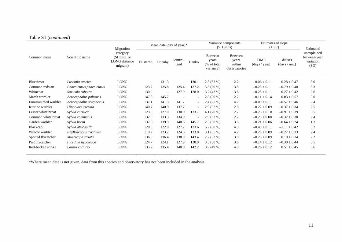
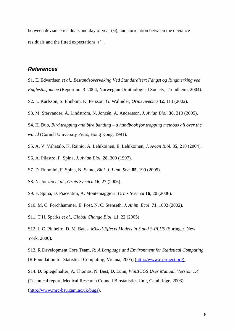
Table S1 (continued)
Mean date (day of year)* Variance components (SD units)
Estimates of slope (± SE)
Common name Scientific name
Migration category
(SHORT or LONG distance
migrant) Falsterbo Ottenby Jomfru-
land Hanko
Between years
(% of total variance)
Between years within
observatories
TIME (days / year)
dNAO (days / unit)
Estimated unexplained
between-year variation
(SD)
Bluethroat Luscinia svecica LONG - 131.3 - 130.1 2.8 (63 %) 2.2 –0.06 ± 0.11 0.28 ± 0.47 3.0 Common redstart Phoenicurus phoenicurus LONG 123.2 125.8 125.4 127.2 3.8 (50 %) 3.8 –0.23 ± 0.11 –0.79 ± 0.40 3.3 Whinchat Saxicola rubetra LONG 130.0 - 127.9 128.0 3.2 (43 %) 3.6 –0.25 ± 0.11 0.27 ± 0.42 2.6 Marsh warbler Acrocephalus palustris LONG 147.8 145.7 - - 2.8 (50 %) 2.7 –0.11 ± 0.14 0.03 ± 0.57 3.0 Eurasian reed warbler Acrocephalus scirpaceus LONG 137.1 141.3 141.7 - 2.4 (25 %) 4.2 –0.09 ± 0.11 –0.57 ± 0.46 2.4 Icterine warbler Hippolais icterina LONG 140.7 140.9 137.7 - 2.9 (52 %) 2.8 –0.22 ± 0.09 –0.37 ± 0.34 2.5 Lesser whitethroat Sylvia curruca LONG 123.0 127.0 130.9 133.7 4.1 (70 %) 2.7 –0.23 ± 0.10 –0.91 ± 0.39 3.5 Common whitethroat Sylvia communis LONG 132.0 133.3 134.9 - 2.9 (53 %) 2.7 –0.23 ± 0.08 –0.32 ± 0.30 2.4 Garden warbler Sylvia borin LONG 137.6 139.9 140.5 145.7 2.3 (30 %) 3.6 –0.21 ± 0.06 –0.64 ± 0.24 1.3 Blackcap Sylvia atricapilla LONG 120.0 122.0 127.2 133.6 5.2 (60 %) 4.3 –0.49 ± 0.11 –1.11 ± 0.42 3.2 Willow warbler Phylloscopus trochilus LONG 119.2 123.2 124.3 133.8 3.1 (35 %) 4.2 –0.28 ± 0.09 –0.27 ± 0.33 2.4 Spotted flycatcher Muscicapa striata LONG 136.9 136.4 138.0 143.4 2.7 (33 %) 3.8 –0.23 ± 0.09 0.10 ± 0.34 2.2 Pied flycatcher Ficedula hypoleuca LONG 124.7 124.1 127.9 128.9 3.5 (50 %) 3.6 –0.14 ± 0.12 –0.38 ± 0.44 3.5 Red-backed shrike Lanius collurio LONG 135.2 135.4 140.0 142.2 3.9 (49 %)
4.0 –0.26 ± 0.12
0.51 ± 0.45
3.6
*Where mean date is not given, data from this species and observatory has not been included in the analysis.
11
Table S2. Species and observatory specific parameter estimates and variance components when analyzing the middle phase of migration (50th percentile) using a linear mixed model with ‘observatory’ as a fixed effect and a random between-year variance component in common for all observatories.
Mean date (day of year)* Variance components (SD units)
Estimates of slope (± SE)
Common name Scientific name
Migration category
(SHORT or LONG distance
migrant) Falsterbo Ottenby Jomfru-
land Hanko
Between years
(% of total variance)
Between years within
observatories
TIME (days / year)
dNAO (days / unit)
Estimated unexplained
between-year variation
(SD)
White wagtail Motacilla alba SHORT
124.5 129.4 117.0 112.5 0.0 (0 %) 7.6 0.07 ± 0.19 0.31 ± 0.64 0.0 Winter wren Troglodytes troglodytes SHORT 107.2 108.4 - - 1.5 (6 %) 5.8 –0.07 ± 0.12 –0.68 ± 0.45 1.5 Hedge accentor Prunella modularis SHORT 106.8 100.2 103.1 - 4.1 (42 %) 4.8 –0.03 ± 0.14 –0.40 ± 0.53 4.2 European robin Erithacus rubecula SHORT 109.4 112.6 - - 4.7 (74 %) 2.8 0.04 ± 0.15 0.20 ± 0.55 4.9 Common blackbird Turdus merula SHORT 106.0 91.3 - - 1.6 (4 %) 8.1 –0.06 ± 0.17 0.04 ± 0.64 2.4 Song thrush Turdus philomelos SHORT 110.1 111.4 107.6 113.1 3.3 (26 %) 5.5 –0.11 ± 0.12 0.07 ± 0.46 3.4 Redwing Turdus iliacus SHORT 100.7 104.4 103.4 - 3.4 (22 %) 6.5 –0.22 ± 0.16 –1.18 ± 0.58 1.8 Chiffchaff Phylloscopus collybita SHORT 117.0 123.7 119.1 125.6 3.1 (26 %) 5.3 –0.40 ± 0.09 –0.15 ± 0.32 1.2 Goldcrest Regulus regulus SHORT 96.9 112.6 99.7 - 3.1 (24 %) 5.5 –0.06 ± 0.13 0.01 ± 0.48 3.3 Blue tit Parus caeruleus SHORT 91.0 90.5 - - 0.0 (0 %) 5.8 –0.03 ± 0.32 0.05 ± 0.85 0.0 Great tit Parus major SHORT 90.1 87.5 - - 5.1 (71 %) 3.2 –0.07 ± 0.16 –1.12 ± 0.64 4.9 Chaffinch Fringilla coelebs SHORT 105.8 109.4 - 112.4 1.8 (9 %) 5.7 0.13 ± 0.10 –0.49 ± 0.38 1.6 Brambling Fringilla montifringilla SHORT - 116.9 - 113.0 0.0 (0 %) 4.7 –0.02 ± 0.12 –0.58 ± 0.45 0.0 European greenfinch Carduelis chloris SHORT 118.8 114.0 - - 0.0 (0 %) 10.0 0.39 ± 0.19 1.08 ± 0.77 0.0 Common linnet Carduelis cannabina SHORT 127.5 128.0 - - 1.2 (3 %) 6.5 0.09 ± 0.21 –0.76 ± 1.09 1.2 Yellowhammer Emberiza citrinella SHORT - 98.1 - - - 6.4 –0.15 ± 0.30 –0.32 ± 0.89 6.9 Reed bunting Emberiza schoeniclus SHORT 128.1 127.6 108.2 - 8.3 (75 %) 4.9 0.23 ± 0.31 1.21 ± 1.07 9.6 Barn swallow Hirundo rustica LONG - 148.9 147.2 138.9 2.8 (28 %) 4.6 –0.29 ± 0.10 –0.75 ± 0.39 2.0 Tree pipit Anthus trivialis LONG 128.2 131.6 129.1 127.5 3.2 (35 %) 4.4 –0.23 ± 0.11 –0.59 ± 0.41 2.8 Thrush nightingale Luscinia luscinia LONG 137.2 137.8 - - 2.3 (47 %) 2.4 0.04 ± 0.13 –0.10 ± 0.41 2.6
12

Table S2 (continued)
Mean date (day of year)* Variance components (SD units)
Estimates of slope (± SE)
Common name Scientific name
Migration category
(SHORT or LONG distance
migrant) Falsterbo Ottenby Jomfru-
land Hanko
Between years
(% of total variance)
Between years within
observatories
TIME (days / year)
dNAO (days / unit)
Estimated unexplained
between-year variation
(SD)
Bluethroat Luscinia svecica LONG - 135.6 - 136.5 2.7 (57 %) 2.3 0.01 ± 0.11 0.76 ± 0.44 2.8 Common redstart Phoenicurus phoenicurus LONG 134.4 136.6 134.0 135.2 4.0 (53 %) 3.8 –0.18 ± 0.12 –0.78 ± 0.43 3.7 Whinchat Saxicola rubetra LONG 133.0 - 135.9 135.3 2.0 (14 %) 4.8 –0.13 ± 0.12 –0.68 ± 0.44 1.5 Marsh warbler Acrocephalus palustris LONG 149.6 151.9 - - 3.8 (79 %) 1.9 –0.28 ± 0.13 –0.14 ± 0.54 3.4 Eurasian reed warbler Acrocephalus scirpaceus LONG 146.8 151.4 153.7 - 2.9 (35 %) 3.9 –0.15 ± 0.12 –0.03 ± 0.48 3.0 Icterine warbler Hippolais icterina LONG 149.3 149.0 144.4 - 2.1 (32 %) 3.0 –0.15 ± 0.08 –0.34 ± 0.30 1.9 Lesser whitethroat Sylvia curruca LONG 132.1 136.7 139.6 144.8 3.1 (35 %) 4.2 –0.05 ± 0.10 –0.61 ± 0.39 3.1 Common whitethroat Sylvia communis LONG 140.8 144.4 144.2 - 2.8 (41 %) 3.4 –0.09 ± 0.09 –0.44 ± 0.35 2.7 Garden warbler Sylvia borin LONG 145.2 146.9 148.0 153.5 2.6 (34 %) 3.5 –0.19 ± 0.08 –0.47 ± 0.29 2.0 Blackcap Sylvia atricapilla LONG 132.3 135.2 138.5 147.9 4.4 (37 %) 5.7 –0.22 ± 0.15 –0.62 ± 0.54 4.1 Willow warbler Phylloscopus trochilus LONG 130.8 134.8 135.0 145.2 2.4 (27 %) 4.1 –0.20 ± 0.08 –0.54 ± 0.28 1.8 Spotted flycatcher Muscicapa striata LONG 140.7 144.3 146.4 150.5 3.9 (58 %) 3.3 –0.04 ± 0.13 –0.41 ± 0.47 4.0 Pied flycatcher Ficedula hypoleuca LONG 132.0 133.4 137.6 138.8 5.2 (69 %) 3.5 0.11 ± 0.16 –0.56 ± 0.61 5.3 Red-backed shrike Lanius collurio LONG 142.6 145.6 150.2 152.5 3.5 (41 %)
4.3 –0.10 ± 0.13
0.14 ± 0.48
3.7
*Where mean date is not given, data from this species and observatory has not been included in the analysis.
13

Table S3. Species and observatory specific parameter estimates and variance components when analyzing the late phase of migration (90th percentile) using a linear mixed model with ‘observatory’ as a fixed effect and a random between-year variance component in common for all observatories.
Mean date (day of year)* Variance components (SD units)
Estimates of slope (± SE)
Common name Scientific name
Migration category
(SHORT or LONG distance
migrant) Falsterbo Ottenby Jomfru-
land Hanko
Between years
(% of total variance)
Between years within
observatories
TIME (days / year)
dNAO (days / unit)
Estimated unexplained
between-year variation
(SD)
White wagtail Motacilla alba SHORT
154.8 160.9 132.0 121.8 0.0 (0 %) 5.4 0.00 ± 0.13 0.23 ± 0.45 0.0 Winter wren Troglodytes troglodytes SHORT 120.9 124.2 - - 5.1 (80 %) 2.6 –0.32 ± 0.14 –0.25 ± 0.52 4.7 Hedge accentor Prunella modularis SHORT 129.9 114.0 119.9 - 2.4 (10 %) 7.4 –0.14 ± 0.14 –0.48 ± 0.52 2.4 European robin Erithacus rubecula SHORT 119.7 123.2 - - 5.9 (90 %) 2.0 –0.46 ± 0.15 –0.19 ± 0.55 5.1 Common blackbird Turdus merula SHORT 140.3 109.5 - - 0.0 (0 %) 6.7 –0.12 ± 0.13 –0.51 ± 0.49 0.0 Song thrush Turdus philomelos SHORT 123.1 126.5 124.5 128.4 1.3 (2 %) 8.5 –0.16 ± 0.13 –0.53 ± 0.47 1.3 Redwing Turdus iliacus SHORT 101.4 116.8 114.6 - 2.0 (10 %) 6.1 –0.46 ± 0.12 –0.44 ± 0.45 0.0 Chiffchaff Phylloscopus collybita SHORT 137.1 149.0 133.0 142.9 3.1 (14 %) 7.5 –0.33 ± 0.12 –0.42 ± 0.47 2.2 Goldcrest Regulus regulus SHORT 108.5 123.2 114.5 - 4.9 (27 %) 8.2 –0.29 ± 0.19 –0.26 ± 0.71 4.8 Blue tit Parus caeruleus SHORT 114.5 104.2 - - 0.0 (0 %) 9.6 0.05 ± 0.51 –1.57 ± 1.33 2.6 Great tit Parus major SHORT 114.7 102.2 - - 0.0 (0 %) 9.3 0.26 ± 0.21 –0.22 ± 0.87 0.0 Chaffinch Fringilla coelebs SHORT 136.5 140.9 - 126.0 1.1 (2 %) 8.4 0.03 ± 0.14 –0.32 ± 0.53 1.7 Brambling Fringilla montifringilla SHORT - 123.0 - 120.7 0.5 (1 %) 5.2 –0.11 ± 0.12 –1.28 ± 0.45 0.0 European greenfinch Carduelis chloris SHORT 145.4 142.4 - - 5.7 (35 %) 7.9 0.41 ± 0.21 1.06 ± 0.82 4.7 Common linnet Carduelis cannabina SHORT 147.2 154.4 - - 0.0 (0 %) 7.2 0.67 ± 0.18 0.03 ± 0.93 0.0 Yellowhammer Emberiza citrinella SHORT - 118.8 - - - 6.3 –0.18 ± 0.28 0.81 ± 0.84 6.5 Reed bunting Emberiza schoeniclus SHORT 136.6 143.2 133.2 - 6.7 (100 %) 0.0 –0.13 ± 0.18 1.50 ± 0.66 6.2 Barn swallow Hirundo rustica LONG - 159.2 161.2 150.2 2.2 (16 %) 5.1 –0.20 ± 0.09 –1.26 ± 0.36 0.0 Tree pipit Anthus trivialis LONG 133.4 143.2 140.8 136.1 2.3 (12 %) 6.3 –0.28 ± 0.11 –0.75 ± 0.40 0.0 Thrush nightingale Luscinia luscinia LONG 144.7 146.4 - - 3.5 (56 %) 3.1 –0.11 ± 0.17 –0.44 ± 0.55 3.5
14

Table S3 (continued)
Mean date (day of year)* Variance components (SD units)
Estimates of slope (± SE)
Common name Scientific name
Migration category
(SHORT or LONG distance
migrant) Falsterbo Ottenby Jomfru-
land Hanko
Between years
(% of total variance)
Between years within
observatories
TIME (days / year)
dNAO (days / unit)
Estimated unexplained
between-year variation
(SD)
Bluethroat Luscinia svecica LONG - 140.2 - 141.9 3.8 (83 %) 1.7 0.16 ± 0.13 –0.02 ± 0.53 3.8 Common redstart Phoenicurus phoenicurus LONG 144.2 148.7 143.6 144.7 4.5 (55 %) 4.1 –0.17 ± 0.12 –1.24 ± 0.44 3.7 Whinchat Saxicola rubetra LONG 139.0 - 146.2 147.3 3.3 (50 %) 3.4 –0.12 ± 0.12 –0.73 ± 0.44 3.2 Marsh warbler Acrocephalus palustris LONG 155.1 159.2 - - 3.0 (53 %) 2.9 –0.15 ± 0.14 0.27 ± 0.59 3.2 Eurasian reed warbler Acrocephalus scirpaceus LONG 153.5 160.0 161.7 - 0.0 (0 %) 3.4 –0.10 ± 0.07 –0.02 ± 0.30 0.0 Icterine warbler Hippolais icterina LONG 156.0 157.5 154.6 - 1.8 (30 %) 2.7 –0.16 ± 0.07 0.04 ± 0.26 1.5 Lesser whitethroat Sylvia curruca LONG 147.7 150.5 151.4 156.6 2.8 (23 %) 5.1 0.02 ± 0.10 –0.75 ± 0.37 2.5 Common whitethroat Sylvia communis LONG 151.4 157.2 152.7 - 2.6 (42 %) 3.1 –0.15 ± 0.08 –0.56 ± 0.30 2.2 Garden warbler Sylvia borin LONG 154.0 153.5 157.4 160.9 2.3 (35 %) 3.1 –0.16 ± 0.07 –0.12 ± 0.27 2.0 Blackcap Sylvia atricapilla LONG 148.7 150.5 154.5 159.3 3.3 (37 %) 4.3 –0.09 ± 0.12 –0.26 ± 0.43 3.4 Willow warbler Phylloscopus trochilus LONG 142.1 146.9 146.0 156.4 2.1 (28 %) 3.3 –0.05 ± 0.07 –0.66 ± 0.25 1.7 Spotted flycatcher Muscicapa striata LONG 149.1 153.4 157.0 156.5 4.0 (58 %) 3.4 –0.11 ± 0.13 –0.79 ± 0.47 3.9 Pied flycatcher Ficedula hypoleuca LONG 140.9 142.6 146.0 153.6 3.4 (22 %) 6.4 0.17 ± 0.15 –0.45 ± 0.55 3.2 Red-backed shrike Lanius collurio LONG 150.2 152.8 159.8 161.1 3.4 (50 %)
3.4 0.01 ± 0.12
0.40 ± 0.43
3.5
*Where mean date is not given, data from this species and observatory has not been included in the analysis.
15

Table S4. Species-specific parameter estimates on Capri.
Estimates of slope (± SE)
Species Mean date (day of year)
Standard deviation TIME
(days / year) dNAO
(days / unit)
R2
Early phase of migration (10th percentile) Tree pipit 106.7 4.2 –0.05 ± 0.19 0.47 ± 0.50 0.07 Common redstart 109.2 4.1 –0.23 ± 0.15 –0.06 ± 0.46 0.12 Whinchat 111.7 5.3 –0.28 ± 0.18 0.86 ± 0.56 0.26 Icterine warbler 126.3 3.4 –0.29 ± 0.10 0.58 ± 0.29 0.51 Common whitethroat 114.8 4.0 –0.26 ± 0.13 0.75 ± 0.38 0.38 Garden warbler 121.6 3.0 –0.26 ± 0.09 0.34 ± 0.28 0.41 Willow warbler 105.5 4.4 –0.38 ± 0.15 –0.23 ± 0.45 0.30 Spotted flycatcher 121.3 4.0 –0.12 ± 0.13 1.02 ± 0.40 0.35 Pied flycatcher 107.5 4.7 –0.28 ± 0.16 0.76 ± 0.47 0.30
Middle phase of migration (50th percentile) Tree pipit 117.3 3.8 –0.05 ± 0.16 0.58 ± 0.43 0.13 Common redstart 119.9 3.8 –0.20 ± 0.14 –0.14 ± 0.43 0.11 Whinchat 121.8 4.9 –0.32 ± 0.16 0.76 ± 0.48 0.33 Icterine warbler 134.9 4.3 –0.30 ± 0.14 0.64 ± 0.43 0.35 Common whitethroat 125.7 4.1 –0.28 ± 0.12 0.82 ± 0.38 0.43 Garden warbler 132.2 3.4 –0.27 ± 0.11 0.46 ± 0.33 0.38 Willow warbler 116.4 3.6 –0.34 ± 0.12 –0.20 ± 0.36 0.34 Spotted flycatcher 129.9 4.7 –0.06 ± 0.17 0.94 ± 0.51 0.19 Pied flycatcher 117.5 3.9 –0.23 ± 0.13 0.60 ± 0.40 0.28
Late phase of migration (90th percentile) Tree pipit 127.8 3.7 –0.05 ± 0.15 0.73 ± 0.41 0.20 Common redstart 130.6 3.9 –0.20 ± 0.15 –0.23 ± 0.45 0.10 Whinchat 131.8 4.9 –0.37 ± 0.16 0.73 ± 0.47 0.38 Icterine warbler 143.5 5.7 –0.30 ± 0.20 0.67 ± 0.61 0.21 Common whitethroat 136.7 4.4 –0.30 ± 0.13 0.92 ± 0.40 0.45 Garden warbler 143.0 4.1 –0.27 ± 0.14 0.57 ± 0.42 0.31 Willow warbler 127.2 3.2 –0.31 ± 0.10 –0.16 ± 0.31 0.36 Spotted flycatcher 138.7 5.9 0.00 ± 0.23 0.85 ± 0.69 0.09 Pied flycatcher 127.4 3.6 –0.19 ± 0.13 0.44 ± 0.40 0.20
16

Table S5. Priors for mean passage dates on Capri. The parameters τ were constrained to fall within the intervals indicated for each species by using a uniform prior. The range of estimated values of τ (based on the medians of the posterior distributions over all years) are shown to the right.
Species Earliest allowed mean date
Latest allowed mean date
Range in estimated mean date
Tree pipit March 25 May 10 April 21–May 6
Common redstart March 10 May 15 April 24–May 6
Whinchat April 5 May 20 April 23–May 11
Icterine warbler April 25 May 25 May 7–May 21
Common whitethroat March 25 May 25 April 29–May 14
Garden warbler April 15 May 30 May 8–May 17
Willow warbler March 15 May 15 April 20–May 3
Spotted flycatcher April 20 May 25 May 3–May 18
Pied flycatcher April 15 May 20 April 19–May 2
17


![Lienhard Garnier 2009 EtudeCollectionRodin [Edal1]...Nicolas Grimal (Paris) Jean Leclant (Paris) William Kelly Simpson (Katonah, NY) DIRECTOR & EDITOR-IN-CHIEF Patrizia Piacentini](https://img.pdfslide.us/doc/110x75/5e598664d6071906ba090752/lienhard-garnier-2009-etudecollectionrodin-edal1-nicolas-grimal-paris-jean.jpg)