3rd Spanish solar and heliospheric physics meeting, Granada, June, 20113rd Spanish solar and heliospheric physics meeting, Granada, June, 2011

3rd Spanish solar and heliospheric meeting, Granada, 9 June, 2011

assessing modern magnetographs

jose carlos del toro iniesta (SPG, IAA-CSIC)valentín martínez pillet (IAC)

3rd Spanish solar and heliospheric meeting, Granada, 9 June, 2011

what this talk is all about• assessment of the capabilities of modern spectropolarimeters

and magnetographs

• useful during design (tolerances) and exploitation phases (uncertainties)

• pair of nematic LCVR-based instruments (IMaX & SO/PHI)

• demonstrate that they can reach optimum εi regardless of the optics between the modulator and the analyzer

• obtain values for optimum retardances

• derive formulae for

• detection thresholds for B and vLOS depending on the S/N and εi

• inaccuracies and instrument instabilities

3rd Spanish solar and heliospheric meeting, Granada, 9 June, 2011

an optimum polarimeter

• a modulator made up of two nematic LCVRs can be optimum (martínez pillet et al., 2004)

• if axes are at 0º and 45º with S2 > 0 direction

• ideally maximum efficiencies can be reached for both vector and longitudinal analyses

• instrumental polarization may corrupt efficiencies

• we show that ideal efficiencies can be reached by simply tuning voltages

• we first demonstrate that the ideal result can be reached for the single polarimeter

3rd Spanish solar and heliospheric meeting, Granada, 9 June, 2011

polarimetric efficiencies (i)

• (ε1,ε2,ε3,ε4) ≤ (1,1/√3,1/√3,1/√3) (del toro iniesta & collados, 2000)

• 2 nematic LCVRs especially good (martínez pillet et al., 1999)

• optimum theoretical modulation with four measurements: M1 = R(0,ρ); M2 = R(π/4,τ); M4 = L(0); M ≡ M4 M2 M1 ⇒

Oij = (1, cos τi, sin ρi sin τi, - cos ρi sin τi)

• optimum longitudinal modulation (I -/+ V): M1 = R(0,0); M2 = R(π/4,±π/2); M4 = L(0)

M1 M2 M4

3rd Spanish solar and heliospheric meeting, Granada, 9 June, 2011

polarimetric efficiencies (i)

• (ε1,ε2,ε3,ε4) ≤ (1,1/√3,1/√3,1/√3) (del toro iniesta & collados, 2000)

• 2 nematic LCVRs especially good (martínez pillet et al., 1999)

• optimum theoretical modulation with four measurements: M1 = R(0,ρ); M2 = R(π/4,τ); M4 = L(0); M ≡ M4 M2 M1 ⇒

Oij = (1, cos τi, sin ρi sin τi, - cos ρi sin τi)

• optimum longitudinal modulation (I -/+ V): M1 = R(0,0); M2 = R(π/4,±π/2); M4 = L(0)

M1 M2 M4

| || || |

3rd Spanish solar and heliospheric meeting, Granada, 9 June, 2011

polarimetric efficiencies (ii)• the etalon, a retarder: M3 = R(ϑ,δ)

• M = M4 M3 M2 M1 ⇒ Oij = M1j (τi,ρi) ➔ M1j (τi,ρi)

= ±1/√3, j = 2,3,4, are transcendental equations with solution and M11 = 1 ➔ optimum polarimetric efficiencies can be achieved

• trivial cases: ϑ = 0,π/2; δ = 0

M1 M2 M4

3rd Spanish solar and heliospheric meeting, Granada, 9 June, 2011

polarimetric efficiencies (ii)• the etalon, a retarder: M3 = R(ϑ,δ)

• M = M4 M3 M2 M1 ⇒ Oij = M1j (τi,ρi) ➔ M1j (τi,ρi)

= ±1/√3, j = 2,3,4, are transcendental equations with solution and M11 = 1 ➔ optimum polarimetric efficiencies can be achieved

• trivial cases: ϑ = 0,π/2; δ = 0

M1 M2 M4M3

3rd Spanish solar and heliospheric meeting, Granada, 9 June, 2011

polarimetric efficiencies (ii)

3rd Spanish solar and heliospheric meeting, Granada, 9 June, 2011

polarimetric efficiencies (iii)

• a train of mirrors (no matter the number and the relative angles) has a Mueller matrix like (Collet)

• all modulation matrix elements turn out to be multiplied by (a+b) ➔ no effect on the result!

• since mirrors are retarders plus partial polarizers, any differential absorption effect is included

• calibration necessary for non-ideal instruments

M1 M2 M4

E =

!

""#

a b 0 0b a 0 00 0 c d0 0 !d f

$

%%&

3rd Spanish solar and heliospheric meeting, Granada, 9 June, 2011

polarimetric efficiencies (iii)

• a train of mirrors (no matter the number and the relative angles) has a Mueller matrix like (Collet)

• all modulation matrix elements turn out to be multiplied by (a+b) ➔ no effect on the result!

• since mirrors are retarders plus partial polarizers, any differential absorption effect is included

• calibration necessary for non-ideal instruments

M1 M2 M4M3 E

E =

!

""#

a b 0 0b a 0 00 0 c d0 0 !d f

$

%%&

3rd Spanish solar and heliospheric meeting, Granada, 9 June, 2011

noise in action (i)

• we only measure photons ➔ everything depends on photometric accuracy (syst. errors ideally absent)

• noise: limiting factor ⇒

• signal-to-noise ratio ⇒

• detectability is smaller in polarimetry than in pure phototmetry

(S1, S2, S3, S4) ! (I, Q, U, V ) !Siv ,B,!," ! "i

(S/N)i =!

S1

!i

"

c(S/N)i =

!i

!1(S/N)1

martínez pillet et al. (1999) and del toro iniesta & collados (2000)

!i !"

3!1

3rd Spanish solar and heliospheric meeting, Granada, 9 June, 2011

magnetographic inaccuracies (i)

• magnetographic formulae

• error propagation yields

• if S/N = (S/N)1 = 1700 (1000 for S2, S3, and S4) then δ(Blon) = 5 G and δ(Btran) = 80 G for IMaX

• T, V, and other instabilities and defects of LCVRs ⇒ changes in the retardances ⇒ demodulation changes ⇒ cross-talk between the Stokes parameters ⇒ covariances (asensio ramos &

collados, 2008)

Blon = klonVs

S1,cBtran = ktran

!Ls

S1,candLs !

1n!

n!!

i=1

"S2

2,i + S23,iVs !

1n!

n!!

i=1

ai |S4,i |,

!(Blon) =klon

S/N"1

"4!(Btran) = ktran

!"1/"2

S/N= ktran

!"1/"3

S/Nand

3rd Spanish solar and heliospheric meeting, Granada, 9 June, 2011

magnetographic inaccuracies (ii)

• efficiency variances can be seen as functions of retardance variances (del Toro Iniesta & Collados 2000)

• retardance variances can be written as functions of birefringence, thickness, and wavelength variances

• birefringence variance is a sum of thermal and voltage variances

!2max,i =

!4j=1 O2

j i

Np! "!2

max,i= f ("2

"j,"2

#j)

!2!L

"2L

=!2"

#2 +!2

t

t2 +!2#0

$20

!2! = q2

T!2T + q2

V!2V

IMaX

0.3 K or 1.2 mV instabilities induce a 5 % repeatability error in Blon and a 2.5 % repeatability error in Btran

3rd Spanish solar and heliospheric meeting, Granada, 9 June, 2011

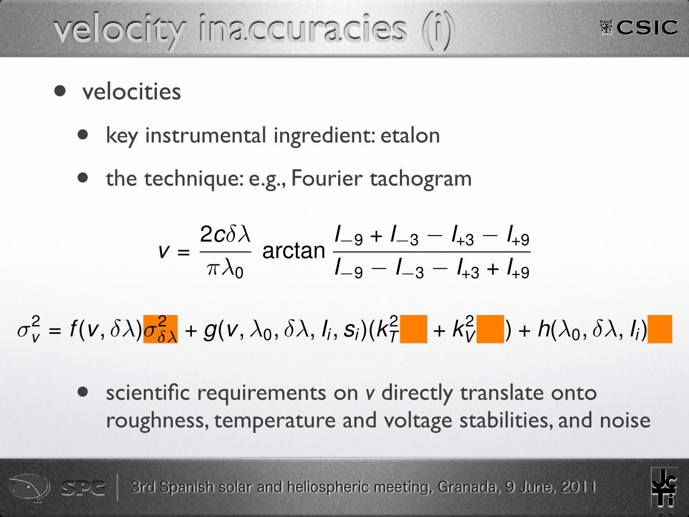
velocity inaccuracies (i)

• velocities

• key instrumental ingredient: etalon

• the technique: e.g., Fourier tachogram

• scientific requirements on v directly translate onto roughness, temperature and voltage stabilities, and noise

v =2c!"

#"0arctan

I!9 + I!3 ! I+3 ! I+9

I!9 ! I!3 ! I+3 + I+9

!2v = f (v , "#)!2

!" + g(v , #0, "#, Ii , si )(k2T !2

T + k2V !2

V ) + h(#0, "#, Ii )!2I

3rd Spanish solar and heliospheric meeting, Granada, 9 June, 2011

velocity inaccuracies (ii)

• assume λ0 = 6173 Å and δλ = 100 mÅ (SO/PHI)

• a roughness instability inducing σδλ = 1 mÅ produces σv = 1 ms-1 for speeds of 100 ms-1! (and is linear in v)

• imagine temperature and noise contribute equally. then, σT/σI = 5.7 and S/N =1700 ⇔ σT = 10 mK

• pure photon noise of σI = 10-3 Ic induces σv = 7 ms-1

• uncertainties larger than 45 mK or 3.4 V produce σv > 100 ms-1 (and this can be an issue for global helioseismology)

!2v = f (v , "#)!2

!" + g(v , #0, "#, Ii , si )(k2T !2

T + k2V !2

V ) + h(#0, "#, Ii )!2I