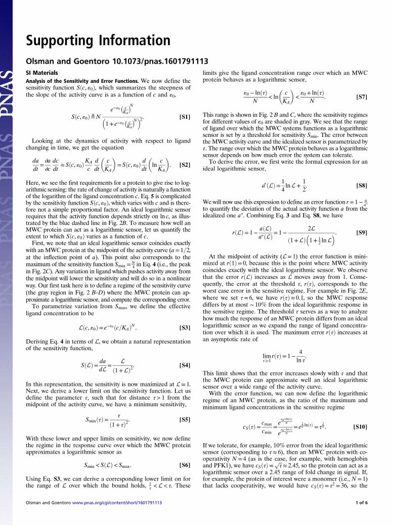
Supporting InformationOlsman and Goentoro 10.1073/pnas.1601791113SI MaterialsAnalysis of the Sensitivity and Error Functions. We now define thesensitivity function Sðc, «0Þ, which summarizes the steepness ofthe slope of the activity curve is as a function of c and «0,

Sðc, «0Þ≜Ne−«0

�cKA

�N�1+ e−«0

�cKA

�N�2. [S1]

Looking at the dynamics of activity with respect to ligandchanging in time, we get the equation

dadt

=∂a∂c

dcdt

≈ Sðc, «0ÞKA

cddt

�cKA

�= Sðc, «0Þ ddt

�ln

cKA

�. [S2]

Here, we see the first requirements for a protein to give rise to log-arithmic sensing: the rate of change of activity is naturally a functionof the logarithm of the ligand concentration c. Eq. 5 is complicatedby the sensitivity function Sðc, «0Þ, which varies with c and is there-fore not a simple proportional factor. An ideal logarithmic sensorrequires that the activity function depends strictly on ln c, as illus-trated by the blue dashed line in Fig. 2B. To measure how well anMWC protein can act as a logarithmic sensor, let us quantify theextent to which Sðc, «0Þ varies as a function of c.First, we note that an ideal logarithmic sensor coincides exactly

with anMWCprotein at the midpoint of the activity curve (a= 1=2,at the inflection point of a). This point also corresponds to themaximum of the sensitivity function Smax = N

4 in Eq. 4 (i.e., the peakin Fig. 2C). Any variation in ligand which pushes activity away fromthe midpoint will lower the sensitivity and will do so in a nonlinearway. Our first task here is to define a regime of the sensitivity curve(the gray region in Fig. 2 B–D) where the MWC protein can ap-proximate a logarithmic sensor, and compute the corresponding error.To parametrize variation from Smax, we define the effective

ligand concentration to be

Lðc, «0Þ= e−«0ðc=KAÞN . [S3]

Deriving Eq. 4 in terms of L, we obtain a natural representationof the sensitivity function,

SðLÞ= dadL=

Lð1+LÞ2. [S4]

In this representation, the sensitivity is now maximized at L= 1.Next, we derive a lower limit on the sensitivity function. Let usdefine the parameter τ, such that for distance τ> 1 from themidpoint of the activity curve, we have a minimum sensitivity,

SminðτÞ= τ

ð1+ τÞ2. [S5]

With these lower and upper limits on sensitivity, we now definethe regime in the response curve over which the MWC proteinapproximates a logarithmic sensor as

Smin < SðLÞ< Smax. [S6]

Using Eq. S3, we can derive a corresponding lower limit on forthe range of L over which the bound holds, 1

τ <L< τ. These

limits give the ligand concentration range over which an MWCprotein behaves as a logarithmic sensor,

«0 − lnðτÞN

< ln�

cKA

�<«0 + lnðτÞ

N. [S7]

This range is shown in Fig. 2 B and C, where the sensitivity regimesfor different values of «0 are shaded in gray. We see that the rangeof ligand over which the MWC systems functions as a logarithmicsensor is set by a threshold for sensitivity Smin. The error betweenthe MWC activity curve and the idealized sensor is parametrized byτ. The range over which the MWC protein behaves as a logarithmicsensor depends on how much error the system can tolerate.To derive the error, we first write the formal expression for an

ideal logarithmic sensor,

apðLÞ= 14lnL+

12. [S8]

Wewill now use this expression to define an error function r= 1− aap

to quantify the deviation of the actual activity function a from theidealized one ap. Combining Eq. 3 and Eq. S8, we have

rðLÞ= 1−aðLÞapðLÞ= 1−

2Lð1+LÞ

�1+ 1

2 lnL�. [S9]

At the midpoint of activity (L= 1) the error function is mini-mized at rð1Þ= 0, because this is the point where MWC activitycoincides exactly with the ideal logarithmic sensor. We observethat the error rðLÞ increases as L moves away from 1. Conse-quently, the error at the threshold τ, rðτÞ, corresponds to theworst case error in the sensitive regime. For example in Fig. 2E,where we set τ= 6, we have rðτÞ≈ 0.1, so the MWC responsediffers by at most ∼ 10% from the ideal logarithmic response inthe sensitive regime. The threshold τ serves as a way to analyzehow much the response of an MWC protein differs from an ideallogarithmic sensor as we expand the range of ligand concentra-tion over which it is used. The maximum error rðτÞ increases atan asymptotic rate of

limτ�1

rðτÞ= 1−4ln τ

.

This limit shows that the error increases slowly with τ and thatthe MWC protein can approximate well an ideal logarithmicsensor over a wide range of the activity curve.With the error function, we can now define the logarithmic

regime of an MWC protein, as the ratio of the maximum andminimum ligand concentrations in the sensitive regime

cSðτÞ= cmax

cmin=e«0+lnðτÞ

N

e«0−lnðτÞ

N

= e2N lnðτÞ = τ

2N . [S10]

If we tolerate, for example, 10% error from the ideal logarithmicsensor (corresponding to τ≈ 6), then an MWC protein with co-operativity N = 4 (as is the case, for example, with hemoglobinand PFK1), we have cSðτÞ= ffiffiffi

τp

≈ 2.45, so the protein can act as alogarithmic sensor over a 2.45 range of fold change in signal. If,for example, the protein of interest were a monomer (i.e., N = 1)that lacks cooperativity, we would have cSðτÞ= τ2 = 36, so the

Olsman and Goentoro www.pnas.org/cgi/content/short/1601791113 1 of 6

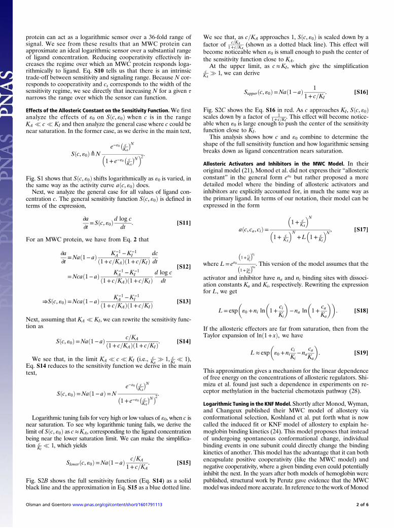
protein can act as a logarithmic sensor over a 36-fold range ofsignal. We see from these results that an MWC protein canapproximate an ideal logarithmic sensor over a substantial rangeof ligand concentration. Reducing cooperativity effectively in-creases the regime over which an MWC protein responds loga-rithmically to ligand. Eq. S10 tells us that there is an intrinsictrade-off between sensitivity and signaling range. Because N cor-responds to cooperativity and cs corresponds to the width of thesensitivity regime, we see directly that increasing N for a given τnarrows the range over which the sensor can function.

Effects of the Allosteric Constant on the Sensitivity Function.We firstanalyze the effects of «0 on Sðc, «0Þ when c is in the rangeKA � c � KI and then analyze the general case where c could benear saturation. In the former case, as we derive in the main text,

Sðc, «0Þ≜Ne−«0

�cKA

�N�1+ e−«0

�cKA

�N�2.

Fig. S1 shows that Sðc, «0Þ shifts logarithmically as «0 is varied, inthe same way as the activity curve aðc, «0Þ does.Next, we analyze the general case for all values of ligand con-

centration c. The general sensitivity function Sðc, «0Þ is defined interms of the expression,

∂a∂t

= Sðc, «0Þ d  log  cdt. [S11]

For an MWC protein, we have from Eq. 2 that

∂a∂t

=Nað1− aÞ K−1A −K−1

I

ð1+ c=KAÞð1+ c=KIÞdcdt

=Ncað1− aÞ K−1A −K−1

I

ð1+ c=KAÞð1+ c=KIÞd  log  c

dt

[S12]

⇒Sðc, «0Þ=Ncað1− aÞ K−1A −K−1

I

ð1+ c=KAÞð1+ c=KIÞ [S13]

Next, assuming that KA � KI, we can rewrite the sensitivity func-tion as

Sðc, «0Þ=Nað1− aÞ c=KA

ð1+ c=KAÞð1+ c=KIÞ. [S14]

We see that, in the limit KA � c � KI (i.e., cKA

� 1, cKI

� 1),Eq. S14 reduces to the sensitivity function we derive in the maintext,

Sðc, «0Þ=Nað1− aÞ=Ne−«0

�cKA

�N�1+ e−«0

�cKA

�N�2.

Logarithmic tuning fails for very high or low values of «0, when c isnear saturation. To see why logarithmic tuning fails, we derive thelimit of Sðc, «0Þ as c≈KA, corresponding to the ligand concentrationbeing near the lower saturation limit. We can make the simplifica-tion c

KI� 1, which yields

Slowerðc, «0Þ=Nað1− aÞ c=KA

1+ c=KA. [S15]

Fig. S2B shows the full sensitivity function (Eq. S14) as a solidblack line and the approximation in Eq. S15 as a blue dotted line.

We see that, as c=KA approaches 1, Sðc, «0Þ is scaled down by afactor of c=KA

1+ c=KA(shown as a dotted black line). This effect will

become noticeable when «0 is small enough to push the center ofthe sensitivity function close to KA.At the upper limit, as c≈KI, which give the simplification

cKA

� 1, we can derive

Supperðc, «0Þ=Nað1− aÞ 11+ c=KI

. [S16]

Fig. S2C shows the Eq. S16 in red. As c approaches KI, Sðc, «0Þscales down by a factor of 1

1+ c=KI. This effect will become notice-

able when «0 is large enough to push the center of the sensitivityfunction close to KI.This analysis shows how c and «0 combine to determine the

shape of the full sensitivity function and how logarithmic sensingbreaks down as ligand concentration nears saturation.

Allosteric Activators and Inhibitors in the MWC Model. In theiroriginal model (21), Monod et al. did not express their “allostericconstant” in the general form e«0 but rather proposed a moredetailed model where the binding of allosteric activators andinhibitors are explicitly accounted for, in much the same way asthe primary ligand. In terms of our notation, their model can beexpressed in the form

aðc, ca, ciÞ=

�1+ c

KA

�N�1+ c

KA

�N+L

�1+ c

KI

�N , [S17]

where L= e«0

�1+ ci

Ki

�ni�1+ ca

Ka

�na. This version of the model assumes that the

activator and inhibitor have na and ni binding sites with dissoci-ation constants Ka and Ki, respectively. Rewriting the expressionfor L, we get

L= exp�«0 + ni   ln

�1+

ciKi

�− na   ln

�1+

caKa

��. [S18]

If the allosteric effectors are far from saturation, then from theTaylor expansion of lnð1+ xÞ, we have

L≈ exp�«0 + ni

ciKi

− nacaKa

�. [S19]

This approximation gives a mechanism for the linear dependenceof free energy on the concentrations of allosteric regulators. Shi-mizu et al. found just such a dependence in experiments on re-ceptor methylation in the bacterial chemotaxis pathway (28).

Logarithmic Tuning in the KNFModel. Shortly after Monod, Wyman,and Changeux published their MWC model of allostery viaconformational selection, Koshland et al. put forth what is nowcalled the induced fit or KNF model of allostery to explain he-moglobin binding kinetics (24). This model proposes that insteadof undergoing spontaneous conformational change, individualbinding events in one subunit could directly change the bindingkinetics of another. This model has the advantage that it can bothencapsulate positive cooperativity (like the MWC model) andnegative cooperativity, where a given binding even could potentiallyinhibit the next. In the years after both models of hemoglobin werepublished, structural work by Perutz gave evidence that the MWCmodel was indeedmore accurate. In reference to the work ofMonod

Olsman and Goentoro www.pnas.org/cgi/content/short/1601791113 2 of 6

et al., Perutz wrote, “These words ring prophetically if we look at themechanism in terms of quaternary structure” (51).Be that as it may, the concept of induced fit proved useful for

describing other classes of allosteric systems, in particular, thosein which negative cooperativity plays an important role (52).Here, we show under what conditions the KNF model can belogarithmically tuned. The KNF model differs from other modelsof binding typically discussed because the specific geometry of theprotein plays an important role, we will use as an example thetetrahedral geometry discussed in the original paper by Koshlandet al. (24), which results in the saturation function

Yðc,KBBÞ=K3AB

cKD

+3K4ABKBB

�cKD

�2+ 3K3

ABK3BB

�cKD

�3+K6

BB

�cKD

�4

1+4K3AB

cKD

+6K4ABKBB

�cKD

�2+4K3

ABK3BB

�cKD

�3+K6

BB

�cKD

�4,

[S20]

where KD is the ligand dissociation constant, and the subunitconformations are denoted A and B. By convention, A will bethe low affinity inactive state and B will be the high-affinity activestate. The interaction strengths KAB and KBB represent the rela-tive strengths of interactions between the A and B conformationsand the B conformation with itself, respectively. Here, we allowallosteric effects to enter through KBB. The motivation for thisassumption is the underlying model that the allosteric effectorsalter the stability of the bonds between the active conformation.The authors use KAA = 1 as a reference interaction strength

against which to measure the other two, so it does not have to beexplicitly accounted for in Eq. S20. In this model, high cooper-ativity comes from high stability of the active state B (i.e.,KBB � 1 and KAB ≈KAA = 1). Under these conditions, the in-termediate terms in the KNF model drop out the saturationfunction and we have the simplified expression

Y ðc,KBBÞ≈K6BB

�cKD

�41+K6

BB

�cKD

�4 =e«0

�cKD

�41+ e«0

�cKD

�4, [S21]

where «0 = 6 lnðKBBÞ. Here, we see that, in the limits of strongcooperativity, the KNF model satisfies the logarithmic tuning re-quirement in relationship 9. This observation is consistent with the dataoriginally fitted by Koshland et al. (24), where they use KAA =KAB = 1and, for the tetrahedral case, find KBB ∈ ½1.8, 6.8�. Even for the lowerend of this range, we have K6

BB ≈ 34, which is much greater thanthe next largest coefficient in Eq. S20, K3

ABK3BB ≈ 5.8.

Detailed Analysis of the GPCR Model. Here, we present a moredetailed derivation of the activation function derived in Eq. 8. Webegin again from the system of differential equations for GPCRactivation:

_R= k1cð1−RÞ− k2R

_TGDP = k3αGDP − k4TGDPR

_TGTP = k4TGDPR− k5TGTP

_αGTP = k5TGTP − k6αGTP

_αGDP = k6αGTP − k3αGDP.

From this system of equations, we will solve for α̂GTP, therelative level αGTP compared with the total level of G proteinTtot =TGDP +TGTP + αGDP + αGTP. Just by setting derivatives equalto zero, we get

α̂GTP =αGTP

Ttot=

αGTP

TGDP +TGTP + αGDP + αGTP

=k5k6TGTP

TGDP +TGTP + αGDP + k5k6TGTP

=k4k6TGDPR

TGDP + k4k5TGDPR+ αGDP + k4

k6TGDPR

=k4k6R

1+ k4k5R+ k4

k3R+ k4

k6R

=R

k6k4+R

�k6k5+ k6

k3+ 1

�.

We then use the fact steady-state relationship

R=c

k2k1+ c

to find

α̂GTP =

ck2k1+ c

k6k4+

ck2k1+ c

�k6k5+ k6

k3+ 1

�

=c

k6k4

�k2k1+ c

�+ c

�k6k5+ k6

k3+ 1

�

=c�

1+ k6k3+ k6

k4+ k6

k5

�c+ k6

k4k2k1

,

just as in Eq. 8. Because k2k1is effectively a KD for the receptors, it

is taken as a fixed quantity. On the other hand, β-arrestin signal-ing alters the rate (k4) at which TGDP binds to active receptors.To this end, we will rewrite Eq. 8 to see whether it can be madeto look like the form described in relationship 9, with thedefinition KD = k2

k1,

α̂GTP =c�

1+ k6k3+ k6

k4+ k6

k5

�c+ k6

k4k2k1

=k4k6

cKD

1+�1+ k6

k3+ k6

k4+ k6

k5

�k4k6

cKD

.

[S22]

Here, we see that, if we allow k4k6to play the role that e«0 plays in

the MWC model, with variations in β-arrestin signaling effec-tively shifting the free energy «, then the GPCR model almostfits the logarithmic tuning requirement in relationship 9. Theconfounding element is the factor of

�1+ k6

k3+ k6

k4+ k6

k5

�that de-

pends on k4 and thus could potentially complicate things. Re-arranging this term, we get

�1+

k6k3

+k6k4

+k6k5

�=�1+ k6

�1k3

+1k4

+1k5

��.

From this equation, we see that there dependence on k4 willvanish so long as either 1

k4� 1

k3+ 1

k5or k6 � k4, and consequently

under these conditions the system will behave as a logarithmicsensor. In terms of the biochemistry of the GPCR pathway, thismeans that β-arrestin binding is far from saturation so that TGDPis always able to find active receptors, be it at an attenuated rate.

Olsman and Goentoro www.pnas.org/cgi/content/short/1601791113 3 of 6

Fold-Change Detection Arises from Logarithmic Sensing and NegativeFeedback. We present here simulations showing fold-change de-tection arising from a circuit containing allosteric regulation andnegative feedback. We use as specific examples the Tar/Tsr re-ceptor system (discussed in Results) and the GPCR system.

Tar/Tsr Receptor and Negative Feedback. We model the allosteric reg-ulation of the receptor using the MWC model and the negativefeedback as described in Shimizu et al. (28) and Pontius et al. (38).The negative feedback via methylation acts on a slower time scalethan receptor activation, such that aðc, «0Þ instantaneously respondsto changes in ligand and allosteric effector concentrations. Further-more, «0 and a are related by a linear feedback coupling, such that

aðc, «0Þ=

�1+ c

KA

�N�1+ c

KA

�N+ e«0

�1+ c

KI

�N

_«0 =mða− a0Þ,

[S23]

where a0 is the basal activation level to which the system adaptsand m is a constant corresponding to the rate of adaptation.When _«0 = 0, we have a= a0, and the system will show preciseadaptation, as expected. Fig. S4 shows the change in Tar/Tsrreceptor activity (blue) in response to sequential threefold stepincreases in ligand concentration (orange). The system gives

identical responses for all three steps, performing fold-changedetection.

GPCR and Negative Feedback. The dynamics of the GPCR systemare described in the main text (Eq. 8). As described in the maintext, allosteric regulation is implemented through k4, whichcharacterizes the rate of receptor phosphorylation and β-arrestinbinding. Although we could express feedback in terms of k4 di-rectly, we may run into problems because k4 is a reaction rateand therefore must be nonnegative. To avoid running into neg-ative values, we rewrite k4 = βe«0, for some constant β. The dif-ferential equations describing the GPCR system are now

_R= k1cð1−RÞ− k2R_TGDP = k3αGDP − βe«0TGDPR_TGTP = βe«0TGDPR− k5TGTP

_αGTP = k5TGTP − k6αGTP

_αGDP = k6αGTP − k3αGDP

_«0 =mða0 − α̂GTPÞ,

[S24]

where α̂GTP = αGTPTtot

. Fig. S5 shows the response of the GPCR sys-tem to sequential threefold step increase in signal. We see againthat a logarithmic sensor coupled with negative feedback yieldsfold-change detection.

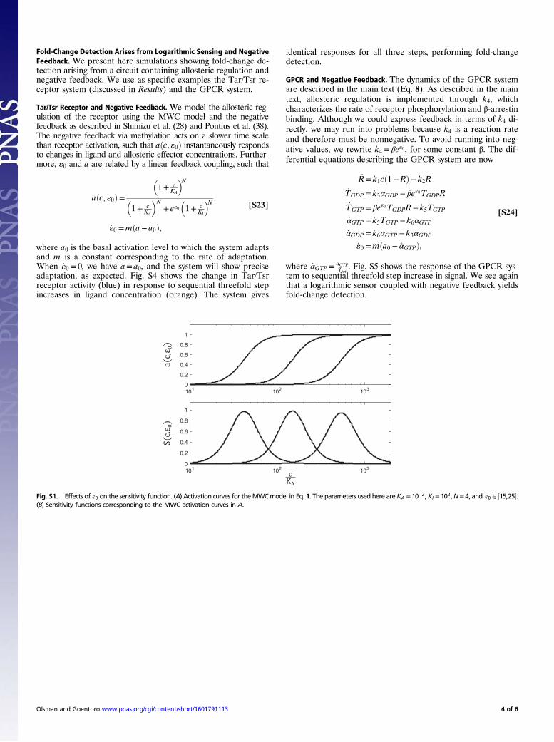
Fig. S1. Effects of «0 on the sensitivity function. (A) Activation curves for theMWCmodel in Eq. 1. The parameters used here areKA = 10−2,KI = 102,N= 4, and  «0 ∈ ½15,25�.(B) Sensitivity functions corresponding to the MWC activation curves in A.

Olsman and Goentoro www.pnas.org/cgi/content/short/1601791113 4 of 6

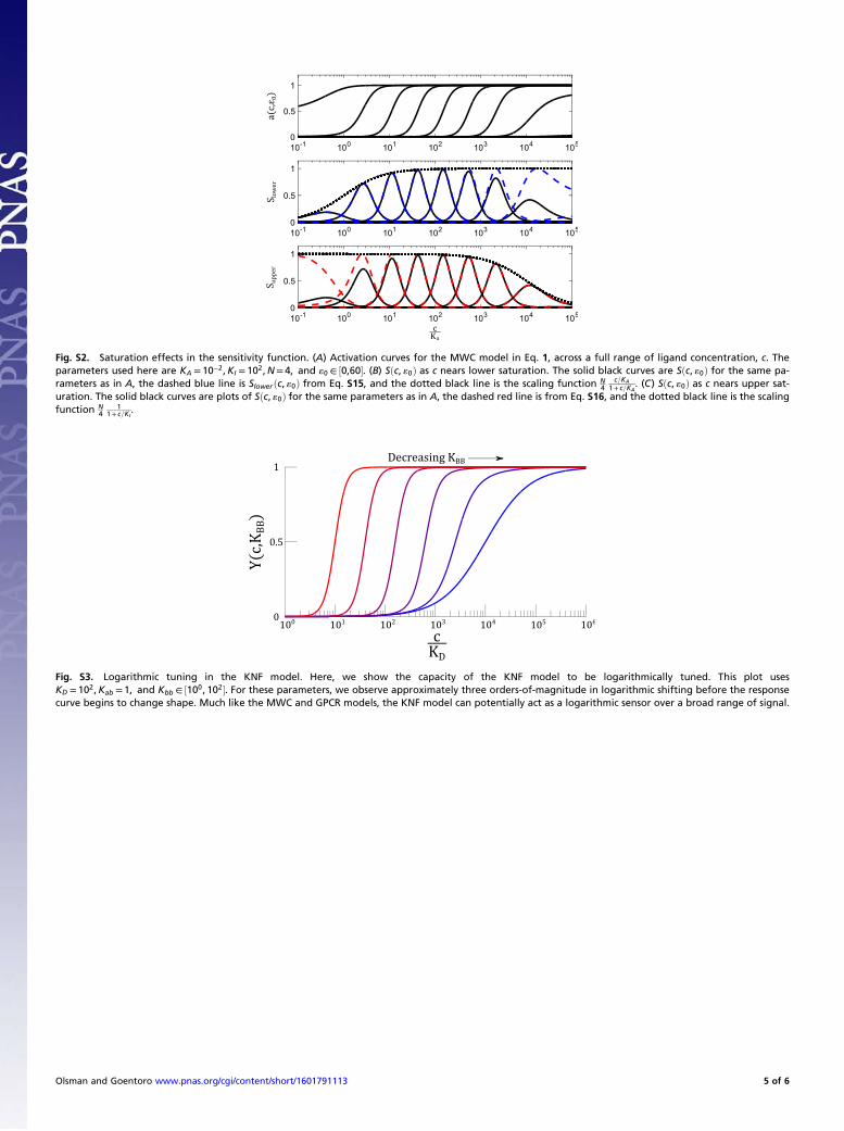
Fig. S2. Saturation effects in the sensitivity function. (A) Activation curves for the MWC model in Eq. 1, across a full range of ligand concentration, c. Theparameters used here are KA = 10−2,KI = 102,N= 4,   and  «0 ∈ ½0,60�. (B) Sðc, «0Þ as c nears lower saturation. The solid black curves are Sðc, «0Þ for the same pa-rameters as in A, the dashed blue line is Slower ðc, «0Þ from Eq. S15, and the dotted black line is the scaling function N

4c=KA

1+ c=KA. (C) Sðc, «0Þ as c nears upper sat-

uration. The solid black curves are plots of Sðc, «0Þ for the same parameters as in A, the dashed red line is from Eq. S16, and the dotted black line is the scalingfunction N

41

1+ c=KI.

Fig. S3. Logarithmic tuning in the KNF model. Here, we show the capacity of the KNF model to be logarithmically tuned. This plot usesKD = 102,Kab = 1,   and  Kbb ∈ ½100, 102�. For these parameters, we observe approximately three orders-of-magnitude in logarithmic shifting before the responsecurve begins to change shape. Much like the MWC and GPCR models, the KNF model can potentially act as a logarithmic sensor over a broad range of signal.

Olsman and Goentoro www.pnas.org/cgi/content/short/1601791113 5 of 6

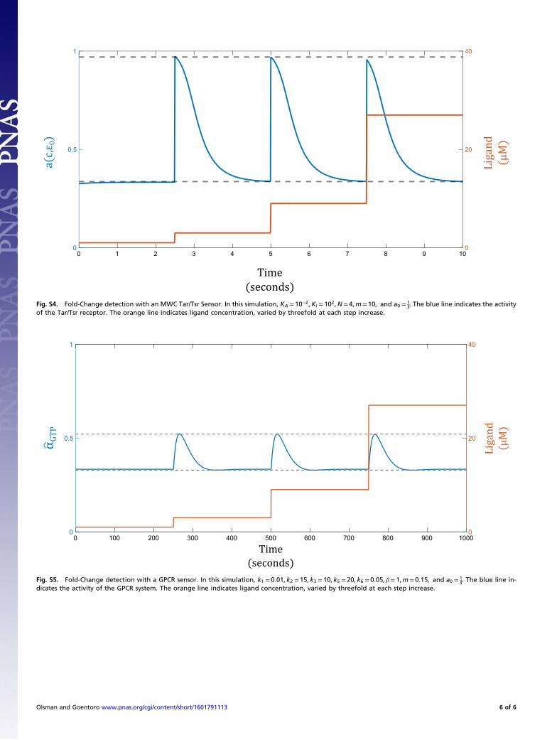
Fig. S4. Fold-Change detection with an MWC Tar/Tsr Sensor. In this simulation, KA = 10−2,KI = 102,N= 4,m= 10,   and  a0 = 13. The blue line indicates the activity

of the Tar/Tsr receptor. The orange line indicates ligand concentration, varied by threefold at each step increase.

Fig. S5. Fold-Change detection with a GPCR sensor. In this simulation, k1 = 0.01, k2 = 15, k3 =10, k5 = 20, k6 = 0.05, β= 1,m= 0.15,   and  a0 = 13. The blue line in-

dicates the activity of the GPCR system. The orange line indicates ligand concentration, varied by threefold at each step increase.

Olsman and Goentoro www.pnas.org/cgi/content/short/1601791113 6 of 6