1

© Copyright 2008, Millennium Press.All rights reserved. Quotation allowed with full attribution.

Supporting Information for “A Climate of Belief” 2008Skeptic 14(1), 22-30

by Patrick Frank

Except as noted, all the calculations and graphics for the work describedhere were done using the application Kaleidagraph (Synergy Software,Reading, PA). The data for article Figure 1, Figure 2, and Figure 3, and forSI Figure 14 and Figure 15 were digitized from the published graphicsusing the program Digitizeit (http://www.digitizeit.de/).

The passive warming model is derived in SI Sections 1 and 2. The goalwas to test outputs of GCMs, and no claim is intended about the actualphysical behavior of climate. In SI Section 1, an estimate is made of thefractional contribution to Earth climate of the enhanced CO2 greenhouseeffect, as modeled in GCMs. The calculation of the enhanced greenhouseeffect of CO2 follows the same assumption made in GCMs, namely thatclimate globally responds with constant relative humidity to the warminginduced by CO2 forcing. Likewise, no claim is made that this assumptionis physically correct. Rather, the condition is included so as to follow thenorms of GCM climate models. In SI Section 2, it is shown that the linearpropagation of this assumption is virtually all that is necessary toreproduce the temperature projections of complex climate models.

SI Section 3 describes the calculation of GCM cloudiness retrodictionerror, and SI Section 4 concerns the description and validation of thepropagation of physical uncertainties in cloudiness and GHG forcing, asapplied to time-wise GCM global average temperature predictions.

SI Sections 5 and 6 discuss the validity of a GCM projection of the 20th

century temperature trend as publicized by the US National Academy ofSciences, and the greening of the Sahel, respectively.

1. Derivation of the Passive Temperature Response Model.

The fractional contribution of the enhanced CO2 greenhouse effect to thetotal greenhouse effect, as portrayed in GCM models, was derived fromasymptotic intercepts of natural logarithmic fits to the data in Table 4,"Equilibrium temperature of the earth's surface (˚K) and the CO2 contentof the atmosphere," of Manabe.1

2

Figure S1: The equilibrium surface temperature under varyingconcentrations of atmospheric CO2, under (), clear skies; fit:T=4.13×ln(CO2)+283.7; r2=0.9999, and ( � ), cloudy skies, fit:T=3.35×ln(CO2)+269.3; r2=0.9999. Data from Manabe.1

The fits plus the fit equations are shown in Figure S1. The functional formof the fit is justified by the natural log relation between greenhouseforcing and the concentration of atmospheric CO2 as given in Myhre, etal.2

The derived greenhouse effect on Earth climate at zero ppm CO2 was thesum of the two asymptotic intercepts (Figure S1) weighted by the ~58.3 %average cloud cover of Earth as determined by integrating the publishedaverage 1983-1990 cloudiness (see article Figure 3 and text). Thus, thezero CO2 greenhouse fraction = 0.583×(269.3 K)+0.417×(283.7 K) =275.3 K. The surface temperature at pure radiation equilibrium = 254.6K, so that the zero CO2 greenhouse contribution = 275.3-254.6=20.7 K.This 21 K represents the greenhouse contribution to Earth surfacetemperature from water vapor alone. The unperturbed total greenhousetemperature (water vapor alone + water-vapor-enhanced CO2) is 33 K.The enhanced CO2 greenhouse contribution is then 33 K-21 K = 12 K.

3

The fractional enhanced greenhouse contribution to Earth surfacetemperature, as represented in GCMs, is thus 12/33=0.36. This methodof weighting by percent cloudy and clear sky forcing has precedent in thederivation of the current average 2.7 W/m2 greenhouse gas forcing inMyhre.2

Figure S2. (), The exponential increase in water vapor pressure withtemperature, and; (−−−), the linear fit From 14-24 C: Vapor Pressure =1.038×T - 2.98; r2= 0.995. The covered range includes the purported risein surface temperature from excess greenhouse warming.

The 0.36×33 C fractional weighting of additional greenhouse forcing inthe model automatically and linearly scales the water-vapor enhancedeffect, already present in the initial 33 C, into the calculated temperatureincreases. Therefore, like all current GCMs, the model automaticallyincludes constant relative humidity. The model approximates the increasein water vapor pressure with temperature as a linear function. Althoughthe true relationship is exponential, the linear increase is a reasonableapproximation over small temperature ranges, Figure S2.

The historical concentrations of CO2 for 1880-1957 were obtained fromEtheridge, et al.,3 and for 1958-2004 were obtained from Keeling andWhorf.4 The historical concentrations of methane were from Etheridge, etal.,5 and of nitrous oxide were from Table 1 in Khalil, et al.6

4

Figure S3 shows the full fits to the historical greenhouse gasconcentrations that were used to calculate greenhouse gas forcings.

Figure S3. Double-y projection of extrapolated atmosphericconcentrations of: (), CO2 (left), and; (−−−), methane and (⋅⋅⋅⋅), nitrousoxide (right). The points are historical measurements.

The fitted equations extrapolating each of the historical greenhouse gasconcentrations in Figure S3 were: For carbon dioxide, CO2 (ppmv)= -6.49×105 + Y×1015.4 - Y2×0.529 + Y3×9.19×10-5, r2=0.996; for methane:CH4 (ppbv) = M0 + M1×Y + ... + M6×Y6 + M7×Y7, where M0=-2.4434×106,M1=12489, M2=-27.119, M3=0.032436, M4=-2.3081×10-5,M5=9.7725×10-9, M6=-2.2801×10-12, M7=2.262×10-16, r2=0.997; fornitrous oxide: N2O (ppbv) = 0.58662×Y - 857.04, r2= 0.977. In all cases,Y is the 4-digit year.

The increasing forcings due to added greenhouse gases calculatedaccording to the equations in Myhre, et al.,2 are shown in Figure S4.

5

Figure S4. Additional greenhouse gas forcing from the year 1900, for:(), CO2; (−−−), methane, and; (⋅⋅⋅⋅), nitrous oxide, as calculated from thefits to the greenhouse gas concentrations of Figure S3, using theequations in Myhre.2

The forcings in Figure S4 were summed in order to calculate theincreased greenhouse temperature in equation S1, as given in ACoB:

Global Warming=0.36x33Cx[(Total Forcing)÷(Base Forcing)] S1,

where “Base Forcing” is the forcing from all three greenhouse gasses ascalculated from their historical or extrapolated concentrations for eitherthe year 1900 or 2000, depending on which year was chosen as thezeroth year. “Total Forcing” is “Base Forcing” + the increase in forcing.

When the temperature increase due to a yearly 1 % CO2 increase wascalculated, the increasing CO2 forcing was adjusted to include the higheratmospheric concentration of this gas, but the increasing forcings due tomethane and nitrous oxide were left unchanged at their Figure S4 values.

1.2 On Origins. An anonymous reviewer of an earlier form of themanuscript suggested that equation S1 is “the standard linearized

6

relation between radiative forcing and global-mean temperatureresponse,” and further stated that the author of ACoB and ACoB SI madea dishonest claim of originality. It is worth reviewing that charge here toforestall any recapitulation of the accusation.

Nowhere in the SI or in the article is any originality claimed. Nor did anysuch claim appear in the prior version of these documents evaluated bythat reviewer. Copies of the prior documents are available.

The reviewer went on to name “the IPCC report,” as one source for thestandard linearized relation. In the 4AR a linear model is discussed inChapter 2, Section 2.8.4, “Linearity of the Forcing-ResponseRelationship,”7 which presumably exemplifies what the reviewer had inmind.

The linear temperature response model given by the IPCC is:

∆Ts=λCO2×Ei×RFi, R1

where Ts is the surface temperature, λCO2 is “the climate sensitivityparameter” for CO2, Ei is the efficacy of some forcing agent “i” defined inrelation to that for CO2, and RFi is the radiative forcing for the ith forcingagent.

The following analysis will show that equation S1 is different fromequation R1.

When the forcing agents are CO2 plus methane plus nitrous oxide -- thegases included in the present analysis -- equation R1 becomes:

∆Ts=(λCO2×RFCO2)+(λCO2×ECH4×RFCH4)+(λCO2×EN2O×RFN2O). R2

Compare R2 to the expanded form of equation S1:

∆Ts=T0×fEGE×[(∆FCO2+∆FCH4+∆FN2O)÷F0], S1’

where Ts is again the surface temperature, T0 is the empiricallydetermined base greenhouse contribution to the surface temperature(i.e., 33 C), fEGE estimates the fractional contribution of the enhanced CO2greenhouse effect to the surface greenhouse temperature, but in themagnitude that fraction has within GCMs as deduced from the resultsreported by Manabe,1 as shown in Figure S1 and discussion, ∆FGAS is thecanonical change in greenhouse gas forcing2 due to the increasedconcentration of each relevant gas after the zeroth year, and F0 is thereference (i.e., the zeroth year total) greenhouse gas forcing.

7

Equations S1 and S1’ are different from equations R1 and R2 in terms oforigination logic, of physical constituents, and of dimensional units. Theapproach to, and constituents of, equation S1 completely reveal itsindependent origin. Equation S1 is not the “the standard linearizedrelation between radiative forcing and global-mean temperatureresponse.” It is not, as is equation R1, a derivation of surface temperaturefrom the physical theory of radiative forcing. Equation S1 is a linearized,empirical, and physically reasonable estimator of what GCMs mightproduce when used to calculate average surface temperature.

Equations S1 and R1 are equivalent merely in linearity and calculationalfocus (i.e., they equate to ∆Ts).

Because S1 and R1 each equate to ∆Ts they must equate to one another,in principle at least. Thus, λCO2×Ei×RFi = T0×fEGE×(∆FGAS÷F0). In this case,there should exist a set of transformations that converts equation S1 intoequation R1.

Equational parity does not translate into derivational identity, however.To exemplify this distinction by citing a famous equivalence: in order tosuppose that equations S1 and R1 are derivationally identical becausethey can be somehow interconverted through ∆Ts, one must also acceptthat Erwin Schrödinger’s a posteriori wave mechanics are derivationallyidentical to Werner Heisenberg’s matrix mechanics because the two haveequational parity through EΨ and can be rigorously interconverted. By thereviewer’s logic, it would have been dishonest for Erwin Schrödinger toclaim originality for his master work. Clearly that logic fails, both hereand above.

Emphatically, no comparison is claimed or implied between the workpresented in the SI and anything Schrödinger or Heisenberg attained.Obviously, there can be no such comparison whatever. What is claimed inthe above example is a powerful illustration of an impoverished andtendentious logic.

No originality is claimed here. Derivational independence is claimed.

2. Passive Model Validation by Comparison with GCMProjections

Here, the passive warming model as detailed above is shown to be closerto the ensemble average of the 10 GCM projections from the CMIP thanany of the individual GCM projections themselves. The test model is a

8

line, while the GCM projections contain excursions from their respectivemeans. In order to remove any bias due to this difference, linear leastsquare fits were made to all 10 GCM projections, so as to determine eachmean projection. The comparison to the ensemble average was thenmade using the passive warming model and the linear means of the 10GCM projections.

Figure S5 reproduces ACoB Figure 2, except that it shows the linearmeans of the 10 GCM projections. In order to make the comparisonquantitative, the Student t-test for paired data sets was used to compareeach of the projections with the 10-GCM ensemble average. Table S1shows the results of this test.

Table S1: Paired Data Student t-Test: 10 GCMs and Passive Model vs.GCM Ensemble Average.

GCMa Mean Difference t-value t-probabilityNCAR 0.171 17.39 <0.0001LMD ISPL -0.111 -14.76 <0.0001HadCM3 -0.223 -25.38 <0.0001HadCM2 -0.046 -11.45 <0.0001GISS 0.125 11.68 <0.0001GFDL -0.175 -11.84 <0.0001ECHAM3 0.106 24.65 <0.0001DOE PCM 0.248 18.74 <0.0001CSIRO -0.144 -18.90 <0.0001CFERACS 0.049 11.12 <0.00011% GHGb 0.014 2.02 0.04496a. Identification of the GCMs represented by the letter codes is in Covey,et al.8 b. Passive greenhouse gas warming model.

In Table S1, “Mean Difference” is the difference between the means of themodel and the ensemble average. A larger absolute value is a greaterdifference. The 1% GHG model is far closer to the ensemble average meanthan any of the GCMs. The “t-value” is the mean difference divided by thestandard deviation of the covariance of the data set - ensemble averagepair. A smaller t-value is a closer correlation. For the “t-probability,” avalue greater than 0.05 means there is no difference between the datasets. Only the passive warming model comes close to meeting this test.

9

Figure S5: As for ACoB Figure 2, except that the GCM projections arerepresented as their linear least square means.

The good correlation between the projections of the passive GHG modeland the projections of complex GCMs (ACoB Figure 2, Figure S5, andTable S1) validates the calculated forcings and the derived enhanced CO2greenhouse fraction of the passive GHG model in terms of the GCMs. Theimplied validity of the inputs in terms of correspondence among theoutputs in turn justifies the SRES error analysis that follows in Section4.1.

The ensemble average of GCM projections has lower intensity excursionsthan any of the GCM projections themselves, as shown in ACoB Figure 2.This means the features in the GCM projections are nearly random, andtend to cancel out when the GCM projections are averaged together.Random features have no physical meaning. If the GCMs were able topredict, e.g., El Niños, it might be expected that at least one intenseevent might show up in 80 years of greenhouse warming oceans, perhapssimilar to the 1998 event.9 GCMs as valid climate models, would allsimilarly predict such an event after a requisite time of heat build-up.This relatively uniform prediction would produce an atmospherictemperature spike in a similar (but perhaps not identical) year in each80-year GCM temperature projection. An El Niño temperature signalwould not cancel like random noise, but would approximately retain its

10

original intensity with the averaging of GCMs and produce a spike in theensemble average trend. There are no such features in the ensembleaverage, and none of the low intensity features remaining are confidentlyassessable as physically real.

3. Cloudiness Retrodiction Error

Table S2 shows the integrated average observed cloudiness of 1983-1990, and the integrated average retrodicted 1979-1988 cloudiness of10 revised GCMs, as taken from Figure 18b of Gates, et al.10

Table S2: Observed and GCM Retrodicted Global Average CloudinessIntegrated Over the Same Pair-Wise Latitudinal Range.

GCMa GCMAverage

Cloudiness

Obs’d. Avg.Cloudiness

AbsoluteFraction

Lag-1 ErrorAutocorrelation

[R]LMD 10629 9647.9 0.10169 0.9631DERF 10389 10291 0.0095164 0.9595BMRC 9050.7 10346 0.12522 0.9881CNRM 10659 10306 0.034217 0.9766NRL 11710 10329 0.13368 0.9850MPI 11353 10313 0.10084 0.9767MRI 11709 10435 0.12206 0.9639DNM 10389 10291 0.0095164 0.9595SUNGEN 10322 10268 0.0052318 0.9411YONU 11972 10436 0.14714 0.9704“Absolute Fraction” = the absolute value of the error fraction [(Observed -GCM)/Observed]. a. Identification of the GCMs represented by the lettercodes is in Gates, et al.10

To obtain the values in Table S2, the observed cloudiness wasinterpolated onto the x-grid of each of the GCM projections, so that inevery case the covered area was identical. The Lag-1 column is discussedin Section 4.2 below.

In each case, the predicted global average cloudiness was the integratedarea of each latitudinal average cloudiness curve for each GCM. Thecomparative integrated area of the observed cloudiness was the observedcloudiness integrated over the same set of latitudes as covered by eachGCM model.

Average GCM error =

€

( [(Obs'd −GCM /Obs'd)2

1

10

∑ ) /9 S2.

11

Thus, error=[√(0.091989/9)]=±0.1011=±10.1%.

The very small absolute errors attending SUNGEN and DERF/DNM arisefor the reason mentioned in the text: the residuals from these projectionshave almost equal positive and negative areas of excursion. A betterestimate of the total error remaining after the 10-averages, calculated asthe integrated √[(residual)2], yields 16.6 % for DERF/DNM and 15.6 % forSUNGEN. For CNRM and YONU, the total error likewise becomes 31.5 %and 29.4 %, respectively.

Each GCM projection considered here is the average of ten yearlycloudiness realizations (1979-1988). The observed cloudiness is an 8-year average. Averaging across the years tends to smooth out the year-to-year variations. The resulting smoothness removes latitudinaleccentricities from both the observed cloudiness and the retrodictedcloudiness. This homogenization of both retrodiction and observationtends to suppress the detection of errors.

4. SRES A2 Error Propagation

4.1 The temperature uncertainty due to cloud error: Cloud error aspresent in the A2 scenario was calculated by first extracting greenhousegas forcings equivalent to those used by the IPCC to calculate the originalA2 scenario. The compatibility of the passive warming model projectionwith real GCM projections (ACoB Figure 2, Figure S5, and Table S1)validates applying the same greenhouse gas forcings as used in thepassive GHG model to the A2 projection.

Therefore, the A2 SRES Total Forcing was estimated as,

(Year 2000 Forcing)×[(A2 Temp+Year 2000 Temp)/(Year 2000 Temp)] S3,

where the Year 2000 Forcing was the total forcing calculated from theconcentrations of CO2, methane, and nitrous oxide at their year 2000levels, using the equations in Myhre, et al.2 The Year 2000 Temp was thetotal increased greenhouse temperature due to the same gasses at theiryear 2000 levels, relative to their known or extrapolated year 1900 levels(see Figures S3 and S4), calculated according to equation S1. This wasadded to the SRES A2 year 2000 temperature, because at year 2000, theA2 projection begins at zero (0) degrees.

So,

"A2 Total Forcing" = (35.163)×(A2 Temp+13.938)/(13.938) S4,

12

where 35.163 is the total greenhouse forcing in the year 2000, in Wm-2,derived according to Figures S3 and S4, and 13.938 is the water-vapor-enhanced greenhouse gas temperature contribution in Celsius at the year2000 as calculated using equation S1. In the A2 projection, the nettemperature increase starts at zero C in the year 2000.

Per Year Cloud Error for SRES A2 for each year is then,

Yearly Error=(A2 Temp+Year 2000 Temp)×[(Cloud Forcing Error/(Total Forcing)] S5,

where A2 Temp is the temperature of the A2 projection in each yearstarting at year 2000, Year 2000 Temp is the surface temperature of theyear 2000 calculated using equation S1, Cloud Forcing Error is ±2.8 Wm-2

as obtained by applying the equation S2 result (see the discussion inACoB), and Total Forcing in Wm-2 is the extracted A2 forcing, ascalculated by equation S4.

4.2 The structure of GCM cloudiness retrodiction residuals: Theaverage cloudiness per latitude as retrodicted by the GCMs (ACoB Figure3) are one-dimensional (univariate) spatial data, which makes themstructurally identical to a linear time series. That allows the unfitresiduals to be tested for autocorrelation using simple one-dimensionalstatistical models. As justified below, the final error propagation model isequivalent to a non-stationary random-walk-like accumulation model inpart justified by an assessment that the statistical structure of the unfitaverage cloudiness residuals are all consistent with unit rootautoregressive models.

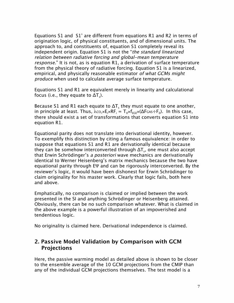
Figure S6 shows the structure of a Lag-1 plot from a random numberseries ranging between zero and 100, used here to illustrate anuncorrelated one-dimensional error series.

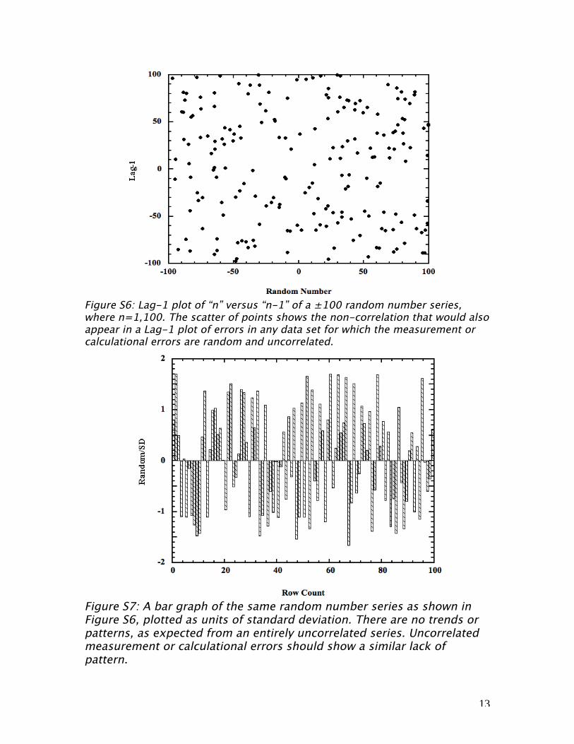
Figure S7 shows the same series as a bar-graph normalized to thestandard deviation (SD) of the series. No pattern emerges. These Figuresdemonstrate how uncorrelated errors should appear to visual inspection.Uncorrelated Gaussian-normal errors do not accumulate in a long set ofiterated outputs from a model.

13

Figure S6: Lag-1 plot of “n” versus “n-1” of a ±100 random number series,where n=1,100. The scatter of points shows the non-correlation that would alsoappear in a Lag-1 plot of errors in any data set for which the measurement orcalculational errors are random and uncorrelated.

Figure S7: A bar graph of the same random number series as shown inFigure S6, plotted as units of standard deviation. There are no trends orpatterns, as expected from an entirely uncorrelated series. Uncorrelatedmeasurement or calculational errors should show a similar lack ofpattern.

14

Figure S8 shows the Lag-1 plot of the unfit residual of the CNRM GCMcloudiness retrodiction shown in ACoB Figure 3. The unfit residual is whatis left when the observed cloudiness is subtracted from the GCMretrodicted cloudiness. In a perfectly accurate retrodiction, the unfitresidual would be a series of zeros. For the CNRM residual, there isevidence of high autocorrelation in the error values; that is, the value ofevery Yn is linearly dependant in some way from the value of thepreceding Yn-1. Autocorrelation means that the CNRM unfit residualincludes at least one uncompensated trend that extends across the entiredata set (there are no outliers). All of the GCM cloudiness error residualsshowed high autocorrelation (Table S2).

Figure S8: (), Lag-1 plot of the unfit residual of the CNRM prediction of1979-1988 average cloudiness, and; (), a linear regression fit to thedata. The negative percents arise when retrodicted cloudiness exceedsobserved cloudiness. Compare with Figure S6.

Figure S9 shows the CNRM unfit residual as a bar-plot. The residualseries of each of the ten GCMs similarly showed a structured profile.These residuals clearly do not have a constant variance (SD2) across theentire data set, and are consistent with non-stationarity.

15

Figure S9: CNRM cloudiness unfit residuals, plotted as (retrodicted minusobserved) cloudiness percent difference. Compare with Figure S7.

Figure S6 through Figure S9 show that the GCM cloudiness retrodictionerrors do not behave as Gaussian random noise. Non-symmetric errorwill not self-cancel across an iteratively calculated series.

Random error cancels as √N as N series are averaged. The random noisecomponent in each 10-year GCM average cloudiness projection shouldalready have been reduced by a factor of about √10=3.16-fold, relative toany Gaussian random noise component in each of the ten 1-yearrealizations of each of the GCM average cloudiness projections. FigureS10 illustrates this effect. If the ±10.1% average cloudiness error was dueto residual random noise that survived the averaging process in each ofthe 10-averages, then the error due to random noise in each 1-year GCMrealization necessarily averages about 3.16 times larger. That is, theaverage cloudiness error due to random excursions alone would be about32%. That means a about ±8.8 Wm-2 uncertainty would be present in

16

every temperature calculation by a GCM. That uncertainty is 3.3× largerthan the effect of all the human-produced greenhouse gasses presentlyin the atmosphere. However, as will be shown below, the ±10.1 % isunlikely to represent random error.

Figure S10: The √N effect of averaging random noise error: (—),random number series between the limits of 1 and -1; (—), theaverage of 10 such series, and; (—), the average of 80 such series.The standard deviations of these specific series have the ratios of 1,0.328 (1/√10=0.316), and 0.120 (1/√80=0.112), respectively.

To further test the structure of the GCM cloudiness error, the correlationmatrix for all ten residual series was calculated using the Student t-Testfor paired data with equal variance. This choice of conditions followsfrom the fact that all the GCMs targeted the same observed cloudiness,all began with similar (if not identical) empirical inputs, and all employedsimilar numerical methods. If each residual series represented randomerrors, their pair-wise correlations should be approximately zero (0). Onthe contrary, the correlation matrix in Table S3 shows that high to veryhigh pair-wise correlations occur very often between unfit residual series.

Again, the correlation between paired series of random errors should bezero (0). However, happenstantial correlation can occur in smallindependent data sets. Tests for happenstantial correlation across somecomputer generated random series of 200 points showed small pair-wise

17

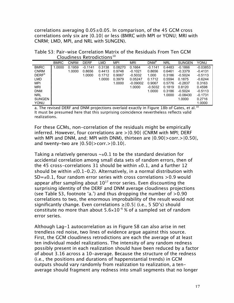
correlations averaging 0.05±0.05. In comparison, of the 45 GCM crosscorrelations only six are |0.10| or less (BMRC with MPI or YONU; MRI withCNRM; LMD, MPI, and NRL with SUNGEN).

Table S3: Pair-wise Correlation Matrix of the Residuals From Ten GCMCloudiness Retrodictions10

BMRC CNRM DERF LMD MPI MRI DNMa NRL SUNGEN YONUBMRC 1.0000 0.1959 -0.1141 0.3138 0.08270 0.1664 -0.1141 0.4483 -0.1866 -0.03853CNRM 1.0000 0.8656 0.4413 0.9748 -0.1021 0.8656 0.6461 -0.3379 -0.4131DERFa 1.0000 0.1712 0.9067 -0.5032 1.000 0.3186 -0.5024 -0.5113LMD 1.0000 0.3979 0.05247 0.1712 0.5594 0.1875 -0.6244MPI 1.0000 -0.09002 0.9067 0.5776 -0.2837 0.3163MRI 1.0000 -0.5032 0.1819 0.8120 0.4598DNM 1.0000 0.3186 -0.5024 -0.5113NRL 1.0000 -0.08430 -0.1731SUNGEN 1.0000 0.2716YONU 1.0000

a. The revised DERF and DNM projections overlaid exactly in Figure 18b of Gates, et al.10

It must be presumed here that this surprising coincidence nevertheless reflects validrealizations.

For these GCMs, non-correlation of the residuals might be empiricallyinferred. However, four correlations are >|0.90| (CNRM with MPI; DERFwith MPI and DNM, and; MPI with DNM), thirteen are |0.90|>corr.>|0.50|,and twenty-two are |0.50|>corr.>|0.10|.

Taking a relatively generous ~±0.1 to be the standard deviation foraccidental correlation among small data sets of random errors, then ofthe 45 cross-correlations 31 should be within ±0.1, and a further 12should be within ±(0.1-0.2). Alternatively, in a normal distribution withSD=±0.1, four random error series with cross correlations >0.9 wouldappear after sampling about 1017 error series. Even discounting thesurprising identity of the DERF and DNM average cloudiness projections(see Table S3, footnote ‘a.’) and thus dropping the number of >0.90correlations to two, the enormous improbability of the result would notsignificantly change. Even correlations ≥|0.5| (i.e., 5 SD’s) shouldconstitute no more than about 5.6×10-6 % of a sampled set of randomerror series.

Although Lag-1 autocorrelation as in Figure S8 can also arise in nettrendless red noise, two lines of evidence argue against this source.First, the GCM cloudiness retrodictions are each the average of at leastten individual model realizations. The intensity of any random rednesspossibly present in each realization should have been reduced by a factorof about 3.16 across a 10-average. Because the structure of the redness(i.e., the positions and durations of happenstantial trends) in GCMoutputs should vary randomly from realization to realization, a ten-average should fragment any redness into small segments that no longer

18

dominate an entire series (if red noise ever did dominate any of theindividual GCM cloudiness projections). This result is not consistent withpersistent Lag-1 behavior through every 10-year average, nor with thedominance of pair-wise residual correlations in Table 3. Second, thedomination of pair-wise correlations across the GCMs residual series(Table S3), in and of itself, also argues against trendless red noise as thesource of the correlations unless it can be shown that GCMs producerandom errors with consistent inter-GCM reddening trends in the samephysical output ranges. In small data sets such uncompensatedcorrelated trends could dominate the residuals and appear as cross-correlations. The necessity of consistently producing correlated randomtrends both inter-GCM and in the same data ranges savages the usualdefinition of “random,” however. These considerations argue againstuncompensated red noise as the source of the observed correlation in theGCM cloudiness residuals.

Instead, the high Lag-1 and GCM pair-wise correlations of residualsimply that the unfit cloudiness residuals derive from systematic errors intheory that are often similarly expressed among GCMs. From Table 3,where they are wrong, GCMs are often wrong in the same way (orinversely, e.g., LMD vs. YONU).

Finally, every residual series was subjected to the Phillips-Perron test forunit roots in the AR(1) autoregressive model,

€

Yl = φYl − 1 + εl + ul , where Yl isthe unfit cloudiness residual at a given latitude, Yl-1 is the latitudinallypreceding datum, φ is the autocorrelation coefficient, εl is white noise,and ul represents a linear latitude-dependent trend in the residuals. If thecoefficient φ=1 (unit root), the series is a non-stationary random walk. Inrandom walks, the error accumulates additively across the series.

Autoregressive models without a trend (ul=0) or with a trend were tested.These tests were carried out by Prof. Ross McKitrick, Department ofEconomics, University of Guelph, whose generosity of time and attentionis acknowledged with gratitude.

The results are presented in Tables S4 and S5.

19

Table S4: Phillips-Perron Unit Root Test without TrendInterpolated Dickey-Fuller % Critical ValueGCM Error Series

P-P Statistic 1% 5% 10%MacKinnon p-value for Z(t)

BMRC Z(ρ)=0.792 -19.422 -13.532 -10.874 ---BMRC Z(t)=0.302 -3.539 -2.907 -2.588 0.9763CNRM Z(ρ)=-1.473 -19.134 -13.404 -10.778 ---CNRM Z(t)=-0.505 -3.562 -2.920 -2.595 0.8296DERF Z(ρ)=-2.911 -19.134 -13.404 -10.778 ---DERF Z(t)-0.848 -3.562 -2.920 -2,595 0.8058LMD Z(ρ)=-12.454 -18.832 -13.268 -10.680 ---LMD Z(t)=-1.846 -3.587 -2.933 -2.601 0.3577MPI Z(ρ)=-1.544 -19.134 -13.404 -10.778 ---MPI Z(t)=-0.526 -3.562 -2.920 -2.595 0.8883MRI Z(ρ)=0.763 -18.900 -13.300 -10.700 ---MRI Z(t)=0.259 -3.500 -2.930 -2.600 0.9744DNM Z(ρ)=2.911 -19.134 -13.404 -10.778 ---DNM Z(t)=-0.848 -3.562 -2.920 -2,595 0.8058NRL Z(ρ)=-0.012 -19.242 -13.452 -10.810 ---NRL Z(t)=-0.017 -3.553 -2.915 -2.592 0.9570SUNGEN Z(ρ)=-3.965 -18.900 -13.300 -10.700 ---SUNGEN Z(t)=-1.056 -3.500 -2.930 -2.600 0.7327YONU Z(ρ)=0.715 -18.628 -13.172 -10.620 ---YONU Z(t)=0.242 -3.607 -2.941 -2.605 0.9736Newey-West lags=3 in all cases.

Table S5: Phillips-Perron Test with TrendInterpolated Dickey-Fuller Percent Critical ValueGCM Error Series

P-P Statistic 1% 5% 10%MacKinnon p-value for Z(t)

BMRC Z(ρ)=1.659 -26.686 -20.322 -17.206 ---BMRC Z(t)=0.729 -4.086 -3.471 -3.163 0.9987CNRM Z(ρ)=0.039 -26.142 -20.034 -16.982 ---CNRM Z(t)=-0.005 -4.121 -3.487 -3.172 0.9955DERF Z(ρ)=-3.112 -26.142 -20.034 -16.982 ---DERF Z(t)=-0.917 -4.121 -3.487 -3.172 0.9545LMD Z(ρ)=-8.113 -25.572 -19.724 -16.752 ---LMD Z(t)=-0.971 -4.159 -3.504 -3.182 0.9479MPI Z(ρ)=-0.550 -26.142 -20.034 -16.982 ---MPI Z(t)=-0.218 -4.121 -3.487 -3.172 0.9924MRI Z(ρ)=2.580 -25.700 -19.800 -16.800 ---MRI Z(t)=1.196 -4.150 -3.500 -3.180 1.0000DNM Z(ρ)=-0.005 -26.142 -20.034 -16.982 ---DNM Z(t) =-0.917 -4.121 -3.487 -3.172 0.9545NRL Z(ρ)=1.678 -26.346 -20.142 -17.066 ---NRL Z(t)=0.761 -4.108 -3.481 -3.169 0.9988SUNGEN Z(ρ)=-3.960 -25.700 -19.800 -16.800 ---SUNGEN Z(t)=-1.093 -4.150 -3.500 -3.100 0.9300YONU Z(ρ)=-0.580 -25.188 -19.496 -16.608 ---YONU Z(t)=-0.218 -4.187 -3.516 -3.198 0.9924Newey-West lags=3 in all cases.

20

In the Phillips-Perron test, the null hypothesis is that φ=1. Verification ofthe null hypothesis is met when the calculated Z(ρ) and Z(t) are largerthan the Dickey-Fuller Critical Value. In every case but one, themagnitudes of both Z(t) and Z(ρ) are indeed much larger than all therespective Dickey-Fuller Critical Values. The exception is Z(ρ) for LMDwith no trend (Table S4), which falls between the 5% and 10% Dickey-Fuller limits, marking a slightly weaker verification (cf. Figure S11).However, Z(t) for this entry is much larger than the Dickey-Fuller values.The same LMD residual series easily passed the unit root test for trendeddata (Table S5, see also Figure S11), as do the rest of the cloud unfitresidual series.

The φ=1 null hypothesis is also verified if p>0.05 for Z(t). In every casebut one (LMD, Table S4), p>0.7 at least and in many cases p>0.9.Overall, then, concluding an autoregressive unit root is strongly validatedfor every series of cloudiness residuals.

An explanation for the LMD result in the Phillips-Perron no-trend test canbe found in Figure S11, which compares the LMD and MPI residual series.All the residual series resembled the MPI residual, except the LMD series.The relatively truncated extension of the latter artificially produced a netlinear slope across the series that behaves as a latitude-dependent trendin the Phillips-Perron test. Hence the somewhat less powerful unit rootresult under the no-trend assumption (Table S4), but the very strong unitroot result when a trend is included in the test (Table S5).

From a statistical perspective, the GCM cloudiness residuals can thus be“considered as a random walk, which is not covariance-stationary,”11 across latitude. This result vitiates a statistical argumentthat cloudiness errors can not accumulate across GCM-derivedpredictions.

These findings can be applied to time-wise temperature projectionerrors. The Phillips-Perron tests show the latitudinal residuals are notconsistent with random error, but with a systematic accumulating error.Systematic error can be deposited into a time-wise 10-year average onlyby a systematic error that is propagated time-wise forward from each 1-year GCM realization.

21

Figure S11: The unfit cloudiness residual for: (), the LMD retrodiction,and; (), the MPI retrodiction. All the other GCM residual seriesresembled the MPI series.

If any autocorrelated latitudinal cloudiness residuals in 1-year GCMrealizations were time-wise uncorrelated in multi-year projections, the1-year latitudinal autocorrelation would be progressively lost duringtime-wise averaging. Cloud error that is latitudinally autocorrelated buttime-forward uncorrelated and Gaussian random would, when time-wiseaveraged, produce relatively smaller residual error excursions in a 10-year average (as in Figure S10), with weakened or absent latitudinal Lag-1 correlations, and with residuals oscillating in some relatively low-intensity fashion about the cloudiness zero difference line when plottedas in Figure S11. But that is not observed in these residuals, neithervisually nor by statistical test. The remaining latitudinal errors in the 10-year averages are in fact strongly autocorrelated (Figure S8, Table S2).

22

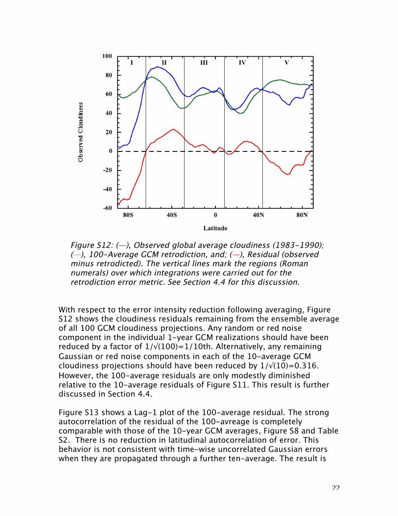
Figure S12: (—), Observed global average cloudiness (1983-1990);(—), 100-Average GCM retrodiction, and; (—), Residual (observedminus retrodicted). The vertical lines mark the regions (Romannumerals) over which integrations were carried out for theretrodiction error metric. See Section 4.4 for this discussion.

With respect to the error intensity reduction following averaging, FigureS12 shows the cloudiness residuals remaining from the ensemble averageof all 100 GCM cloudiness projections. Any random or red noisecomponent in the individual 1-year GCM realizations should have beenreduced by a factor of 1/√(100)=1/10th. Alternatively, any remainingGaussian or red noise components in each of the 10-average GCMcloudiness projections should have been reduced by 1/√(10)=0.316.However, the 100-average residuals are only modestly diminishedrelative to the 10-average residuals of Figure S11. This result is furtherdiscussed in Section 4.4.

Figure S13 shows a Lag-1 plot of the 100-average residual. The strongautocorrelation of the residual of the 100-avreage is completelycomparable with those of the 10-year GCM averages, Figure S8 and TableS2. There is no reduction in latitudinal autocorrelation of error. Thisbehavior is not consistent with time-wise uncorrelated Gaussian errorswhen they are propagated through a further ten-average. The result is

23

consistent, however, with systematic theory-bias errors that remaincorrelated in a time-wise projection and that can be opposinglyexpressed in different GCMs; a trait already indicated by correlations ofresiduals that can be either strongly positive or strongly negative (TableS3).

This reduces or removes the possibility that time-wise (as opposed tolatitudinal) GCM cloudiness errors are uncorrelated or reflect only red-noise trends. The remaining possibility is that the 10-average and 100-average Lag-1 autocorrelations are due to a systematic bias in thecloudiness retrodictions that can propagate forward in a time seriesprojection. Therefore, time-series GCM projections do not produce onlyuncorrelated non-accumulating cloud errors (also see the discussion ofnumerical uncertainty propagation in Section 4.3, the lowest limit theory-bias uncertainty estimate in Section 4.4, and the discussion of time-wisepropagation of Gaussian error in Section 4.5). Cloud-error propagatestime-wise forward, as well as latitudinally, and can accumulate in afutures temperature projection producing an increasing uncertainty.

Figure S13: Lag-1 plot of the residuals remaining from thedifference between the 1983-1990 observed average cloudinessand the further 10-fold ensemble average retrodiction of theoriginal 10-year averaged retrodiction of the 10 GCMs in articleFigure 3.

24

4.3 The theory-bias physical uncertainty propagation model:The coincidence of the line produced by Equation 1 with the linesproduced by the climate models, as displayed in article Figure 2, showsthat increasing forcing propagates linearly through the climate models toproduce increasing temperature. As does the mean value of forcing, themean±(uncertainty) in forcing, i.e., the high/low values of forcingrepresented by the mean±1SD, likewise linearly propagate through themodels to produce ±1SD in calculated temperature.

The statistical analysis of errors in SI Section 4.2 showed that the clouderror was unit root, and so a latitudinal accumulation (Brownian) errormodel was justifiable. The consistent autocorrelation of errors in the 10-and 100-averages showed these errors were very un likely to be time-wise Gaussian. Persistent red noise is unlikely to survive 10- and 100-averages. The error correlation matrix, Table S3, showed that the variousGCMs produced highly correlated errors, which are statistically veryunlikely to be the result of independent random processes. This resultagain implies systematic rather than Gaussian cloud errors. The sameinference turned up in the analysis described in SI Section 4.4 (seebelow), where cloud error does not cancel as expected from a purelyGaussian model, i.e., as 1/√N. The conclusory inference is that the clouderror represents theory-bias, rather than Gaussian noise, and so does notcancel in a time-wise projection.

Proceeding from Section 4.2, assessment of the SRES A2 uncertaintylimits followed a physical model wherein each GCM calculated futuretemperatures as tn=f(t)+e1(tn)+e2(tn), where t=temperature, f(t) is thetemperature generator (e.g., equation S1), e1(t)=statistical error (i.e., themeasurement and numerical errors, each assumed to be Gaussian), ande2(t)=systematic error (i.e., theory bias). This analysis is concerned withthe physical theory-bias errors in GCM projections and so the statisticalerrors, e1(t), were ignored (but see Section 4.5).

In theory-bias error, the modeled value of tn and the physically true valueof tn diverge systematically, continuously, and linearly (at best) by someunknown amount within ±e2(tn) for every iterated new calculation of tn.This error arises because of the inaccuracies, approximations, orincompleteness of the theoretical description.

The justification for the error model described below is that for each prioryear, Yn-1, in a time-wise projection, the climate with its forcings fn-1,represents the initial conditions entering the calculation of the climate ofeach subsequent year Yn, along with the nth year forcings fn. This hasbeen described as “the time-marching method.”12

25

For each year Yn, the limiting values of fn+e2(fn) and fn-e2(fn), empiricallycalculated from the mismatch between prediction and measurement,capture the uncertainty from theory-bias. The resultant discretepredictive divergence of each calculated tn away from the true tn due totheory bias is unknown, but is present in every calculated tn. Because ofthe ambiguity in both the magnitude and the sign of the theory-biaserror, each of which may vary from GCM to GCM, every prediction of anew tn from theory can only be represented by the value range of itstheory-bias uncertainty limits estimated from the difference betweenprojection and observation.

The two limiting uncertainty values of forcing, fn±e2(fn), are themselvesnecessarily valid physical estimates of forcing because they represent theaverage range of the possible magnitude of each fn. That is, the meanmagnitude, fn, does not exhaust the magnitude of the forcing for year Yn.Each of the two limiting values of the uncertainty in calculatedtemperature, i.e., the tn±e2(tn)’s calculated from the fn±e2(fn)’s, are thus asvalid an estimate of the future true tn as the calculated mean tn valueitself. The limiting uncertainty values, fn±e2(fn), therefore cannot beexcluded from a serially iterative projection. Every calculated yearlyforcing, fn (n=1,2,3,…), must thus include the mean value of fn and thehigh and low values of fn representing the average systematic theory-biasuncertainty ±e2(fn), i.e., fn±e2(fn), in each iterative step. The uncertainty inforcing due to theory bias, ±e2(fn), in each Yn then produces anuncertainty in the corresponding calculated temperature tn,.

The yearly modeled increased temperature tn (n=1,2,3,…,n) then equalsthe starting temperature, t0, plus the sum of all the calculated fractionalincreases in temperature, ∆t1,2,…,n. But every ∆t1,2,…,n includes the high andlow values, ±e2(t1,2,…,n), that capture the uncertainty in forcing due totheory bias. These values of ∆t1,2…n±e2(t1,2,…,n) are temperature estimatesthat have a physical validity equal to that of the mean value, ∆t1,2,…,n,itself. All three values, tn, tn+e2(tn) and tn-e2(tn), enter the representationof each new tn and are propagated forward in a time-wise projection, asin S6:

tn=t0+

€

1

n

∑ [∆t1±e2(t1)]+[∆t2±e2(t2)]+[∆t3±e2(t3)]+…+[∆tn±e2(tn)] S6,

where the ∆t1,2…,n is the fractional increase in temperature in Celsius foreach given year n due to increased greenhouse gas forcing ∆fn, and ±e2(tn)contains the high and low physical estimates for ∆tn, based on the ±e2(fn)cloud error or GHG forcing error. This systematic error propagatesadditively with every iteration of a progressive calculation and producesan accumulating uncertainty.

26

The physically modeled temperature projected over time thereforespreads into a vertex of values, with the diameter across the vertexincreasing as the magnitude of ±e2(tn). This vertex captures the predictiveuncertainty in future global temperature.

The cloud forcing error contribution to temperature for each ±e2(tn) wasestimated by equation S5. Estimation of the temperature uncertainty dueto direct uncertainties in GHG forcing proceeded similarly, using theranges given in Myhre.2 Following from the analysis in Section 4.2, thecloudiness error estimate can reasonably be taken to capture a lower-limit average range of theory-bias uncertainty inherent in the 10 GCMsevaluated, which in turn arises from the way cloudiness is physicallyrepresented in these GCMs. Likewise the uncertainty in the GHG forcingwill produce a systematic divergence in predicted and true temperatures,of unknown magnitude but of linear accumulation, which divergence is inturn captured within the forcing uncertainty range.

Thus for SRES scenario A2, the error ±e2(tn) for each year after, e.g., year2000, was calculated as the simple sum of the antecedent errors. Forexample, the total systematic error at, e.g., projection year 100, ±e2(t100),was calculated according to equation S7.

Propagated Error =

€

(peryearn=1

100

∑ clouderror) S7

The total cloud uncertainty for each year includes the error for that yearplus the sum of the errors of the antecedent years, finally summed across100 years for a centennial projection.

4.4 A lowest-limit estimate of cloud theory-bias error: The erroranalysis was extended to the ensemble average of all ten GCM cloudinessretrodictions, shown in Figure S12. This ensemble amounts to a 100-average, i.e., (10 GCMs)×(10 years per GCM).

A standard error of the 100-average was calculated by first dividing thelatitudinal percent cloudiness in Figure S12 into five regions. Theobserved or projected average cloudiness was then integrated in eachregion. The percent error represented by each of the five latitudinalregions was calculated from the integrated residual, as [(observed-retrodicted)/observed]×100, yielding a Δ % error for each region. Theoverall standard error for the 100-average was calculated by the usualformula,

s=

€

[ (Δ%)n2

n=1

5

∑ ]/4 .

27

This error was ±6.0 percent.

For comparison, the direct error calculated as in equation S2 was verycomparable: [(total integrated ensemble cloudiness residual)÷(integratedobserved cloudiness)]×100=6.2%.

This result allows extraction of a lowest-limit estimate for accumulatingtheory-bias error. Suppose, speculatively, that the minimal ±10.1 % errorcalculated in Section 3 was entirely due to uncorrelated noise, rather thandue to the theory-bias that the analysis of Section 4.2 implies. Then thefurther 10-average should have reduced the error magnitude by √10-fold=1/3.16. That is, the 100-average standard error should havebecome (±10.1/√10) %=±3.2 %, if all of the ±10.1 % was due touncorrelated Gaussian noise.

However, the ±10.1 % error instead was reduced to ±6.0 % by the new10-average. That means at most only part of the ±10.1 % could havebeen due to Gaussian noise, while the rest must be due to a systematicerror, namely theory-bias. This theory-bias would represent the veryminimum lowest-limit estimate of GCM theory-bias that could be in thecalculated cloud error, because it is derived from a lower-limit estimateof total cloud error.

If the total error in every case is the sum of an uncorrelated Gaussiannoise component, e1(t), plus a theory-bias component, e2(t), then twolinear equations can be set up:

1. ±[e1(t)+e2(t)]=±0.101, from the individual 10-averages in equation S2.2. ±{[e1(t)/√10]+e2(t)}=±0.060, from the further all-GCM 10-average ofFigures S12 and S13.

Solving these equations for e1(t) and e2(t) yields a lowest-limit estimate ofthe constant average theory-bias error, as well as of the Gaussian noiseerror remaining in the original GCM average cloudiness retrodictions (i.e.,the original 10-averages).

These are: random error = e1(t)=±0.060, and theory-bias error =e2(t)=±0.041, for the respective contributions to the ±10.1 % averageerror as present in each of the original 10-average GCM cloudpredictions.

From that, the average Gaussian noise error, e1(t), in each single-yearGCM cloudiness projection of the ten individual 10-year GCM cloudinessprojections is:

28

GCM per-year projection average e1(t)=±0.06×√10=±0.19, or ±19 %.

This error would also accumulate over an iterative calculation as noted inSection 4.5 below, and is a minimum estimated average uncertaintystemming from the average cloudiness error of the ten GCMs that wouldcontribute to the uncertainty of projected future global temperature,equivalent to an instantaneous global average forcing uncertainty of ±5.3Wm-2.

More interesting is the lowest-limit theory-bias average cloudiness errorestimate of ±4.1 %. This error would accumulate as increasinguncertainty in an iterative calculation, and would not be reduced byperforming arbitrarily large numbers of GCM realizations at each tn-1projection point.

From equation S5, the cloudiness error calculation is linear. Thus, totransfer this lowest limit estimate of theory-bias error to the temperatureuncertainties calculated following Figure 4 in the article, merely multiplythe numbers there by (0.041/0.101)=0.41. That is, the cumulated SRESA2 uncertainties from cloudiness error are reduced to 41% of their Figure4 values.

So, from application of a bare lowest-limit estimate of theory-bias error,the year 2100 SRES A2 projected temperature increase with its associatedphysical uncertainty would be (3.7±46) C. Likewise, after only 4 years theSRES A2 projected warming plus its physical uncertainty would be(0.25±1.8) C, and after 50 years, (1.3±23) C.

That is, even with the lowest-limit estimate of cloud theory-bias error,the accumulating uncertainties make GCM temperature projectionspredictively useless. Our knowledge of future climates is left at zero, evenover the short term.

4.5 An aside about numerical error in GCM temperature projections.As an important aside, the numerical uncertainty in GCM temperatureprojections is typically presented as though it were associated with atime-series of independently measured points, each point havingGaussian error. When data points are independently measured orindependently calculated, the Gaussian error associated with each pointdoes not accumulate across a time-series. However, time-series GCMglobal average temperature projections are not at all like empiricalindependently measured time-series constructions; nor are theyindependently calculated. In a GCM projection, each point, tn, in a time-wise temperature series projection is calculated using the tn-1 point as itsinitial condition. This calculational connection is entirely absent in time-

29

series reconstructions with independent empirically measured orindependently calculated data points, and entirely changes the meaningof the numerical uncertainty in a GCM time-wise climate projection.

For example when employing GCMs to produce the trends in Figure SPM-5, or , e.g., Figure SPM-4 or Figure TS-22 of the 4AR Technical Summary,WG1 and the IPCC are using the mean of each tn-1 point as the initialcondition for calculation of each subsequent tn, but discarding the±(numerical uncertainty) of each tn-1 at each iterated forward step of theGCM temperature projection. Every tn-1 is thus iterated forward as thoughit were perfectly accurate, physically. But this is incorrect. The numericaluncertainty, ±e1(tn-1), is a true uncertainty in the magnitude of eachcalculated temperature, tn-1. That same numerical uncertainty becomes areal physical uncertainty when the calculated temperature tn-1 ispropagated forward to calculate further physical quantities. That is, assoon as each tn-1 is propagated into and through the physical theory of aGCM, its uncertainty is transformed from numerical into physical. Thatmeans the entire numerical uncertainty around each tn-1 becomes a truephysical uncertainty in the magnitude of each tn-1 and must become partof the physical initial state of each subsequent tn. Every ±tn-1 must beincluded in the calculation of each subsequent tn.

In practice, this means the numerical uncertainty accumulates across theyears of a time-wise GCM temperature projection in a manner identical tothe propagation of theory-bias error as described by equation S6 above.The accumulating numerical uncertainty then also produces a wideningvertex of physical uncertainty about the mean temperature series, andthe radius of this vertex increases with the number of projection years.

One could reduce the numerical uncertainty portion of the total physicaluncertainty to an arbitrarily small (±) range by performing an arbitrarilylarge number of GCM realizations at each tn-1. But Gaussian numericaluncertainty only asymptotically approaches zero and would never reachit. The residual numerical uncertainty would always accumulate asphysical uncertainty across an iterative time-wise global averagetemperature projection. Therefore the numerical uncertainty limits aboutthe GCM projected means, as displayed in Figures SPM-4, SPM-5, andTS-22 of the 4AR, are misrepresentations. The part of the total physicaluncertainty in the displayed temperature trends, that which arises fromthe GCM numerical error alone, is far larger than actually presented andrapidly increases across the projected time series.

30

5. Concerning Figure 4 from the U.S. National Academy ofSciences brochure, “Understanding and Responding toClimate Change.”

Cartoon representing the message of Figure 4 from the National Academybrochure, “Understanding and Responding to Climate Change,” datedMarch 2006.13 The blue line is the global surface temperature record. Thegreen lines represent GCM fits under the described forcing assumptions.The inset captions are direct quotes. The validity of this representation iseasily checked by visiting the NAS website at http://dels.nas.edu/basc/ .

31

The original Figure 4 Legend is: “Figure 4. Simulations of pasttemperature more closely match observed temperature when both naturaland human causes are included in the models. The gray [green] linesindicate model results. The red [blue] lines indicate observedtemperatures. Source: Intergovernmental Panel on Climate Change.”

The blue line is the canonical global average surface temperaturerecord.14 The green line is a cartoon representing the message conveyedby the General Circulation Model fit offered by the IPCC. As in NAS figure4, the cartoon version of the GCM fit displays no error bars. TheIPCC/NAS offer the fit as though it has perfect physical accuracy. Onlyvery high physical accuracy can justify the unqualified statements of theinset captions.

How panel 3 of NAS Figure 4 might have looked if it includedthe physical uncertainty of minimal cloud error.

If the NAS/IPCC had opted to display the projection uncertainty due tominimal cloud error, however, panel 3 from Figure 4 might haveappeared as above. The error bars were calculated as described in SISection 4.

32

Minimal cloud error alone would make the uncertainty in the GCMprojection about ±100 C by 1970 and about ±130 C by 2000 relative toclaimed projected temperature anomalies of ~0.4 C and ~0.8 C,respectively.

This unreliability was somehow overlooked by the authors and reviewersof the National Academy of Sciences, as well as by the authors andreviewers of the IPCC.

6. The Greening of the Sahel

The Sahel (the southern borderlands of the Sahara Desert in Africa) hasbeen getting greener.15 The Normalized Difference Vegetation Index(NDVI) of the Sahel is plotted against the trend in atmospheric CO2 inFigure S14. The NDVI is monitored by satellite and measures the changein vegetation. It is reckoned by the authors as particularly suited to studyvegetation changes in semi-arid regions.

The authors looked hard to find an explanation for the greening trend.They wrote: “To conclude, the strong secular trend of increasingvegetation greenness over the last two decades across the Sahel cannotbe explained by a single factor such as climate. Increasing rainfall doesexplain some of the changes but not conclusively. Another potentialexplanation could be improved land management, which has been shownto cause similar changes in vegetation response elsewhere. However, thefact that millet yield and increasing vegetation greenness were unrelateddoes not support this explanation. The third factor, land use changes as aresult of migration, is a plausible contributing explanation, but moreempirical research is needed to verify this.”

At the beginning of their paper, Olsson et al., wrote: “The aim of thispaper is therefore also to discuss and hypothesize possible factors otherthan climate even though we are unable to determine clear linksbetween vegetation change and these factors.” (bolding added)

On the other hand, the correlation r2=0.71 for the concurrent trends inSahel NDVI and atmospheric CO2.

Interestingly, in another article,16 the same authors collaborated withclimate modelers to further study the same question. They showed thatmost of the “aggregated simulated vegetation changes” could beexplained by changes in precipitation. “Aggregated simulated changes”is a revealing description of what was explained. It means that the modelexplained its own predictions, which are only presumed to reflect the

33

same causal chain as those responsible for the greening of the Sahel.

Figure 14: A double-y plot of: (), the greening of the Sahel representedby the NDVI, and; (⋅⋅⋅⋅), the trend in atmospheric CO2, between 1982-1999.

The Sahel NDVI is shown plotted with the Sahel precipitation in FigureS15. The correlation r2=0.33, or less than half that attending the trend inCO2. Part of this difference is due to the smooth yearly CO2 trend, relativeto the jagged yearly variation in precipitation.

However, the correlation r2=0.57 between the trend in Sahel precipitationand atmospheric CO2. So, the correlation between Sahel precipitation andSahel NDVI is partly confounded by the correlation between Sahelprecipitation and atmospheric CO2.

34

Figure S15: A double-y plot of: (), the greening of the Sahelrepresented by the NDVI, and; (⋅⋅⋅⋅), the trend in Sahel precipitationbetween 1982-1998.

Correlation is indeed not causation. But from a political point of view,anyone who claims rising CO2 is causing Earth climate to warm up mustthen insist just as fervently that rising CO2 is causing Earth ecology togreen up.

References :

1. S. Manabe and R. T. Wetherald (1967) Thermal Equilibrium of theAtmosphere with a given Distribution of Relative Humidity Journalof the Atmospheric Sciences 24, 241-259.

2. G. Myhre, E. J. Highwood, K. P. Shine and F. Stordal (1998) Newestimates of radiative forcing due to well mixed greenhouse gasesGeophysical Research Letters 25, 2715-2718.

3. D. M. Etheridge, L. P. Steele, R. L. Langenfelds, R. J. Francey, J.-M.Barnola, et al. (1996) Natural and anthropogenic changes in

35

atmospheric CO2 over the last 1000 years from air in Antarctic iceand firn Journal of Geophysical Research 101, 4115-4128.

4. C. D. Keeling and T. P. Whorf Atmospheric CO2 concentrations(ppmv) derived from in situ air samples collected at Mauna LoaObservatory, Hawaii Scripps Institution of Oceanography (SIO),University of California 2005 http://cdiac.ornl.gov/trends/co2/sio- mlo Last accessed on: 14 September 2007.

5. D. M. Etheridge, L. P. Steele, R. J. Francey and R. L. LangenfeldsHistorical CH4 Records Since About 1000 A.D. From Ice Core Data.In Trends: A Compendium of Data on Global Change CarbonDioxide Information Analysis Center, Oak Ridge NationalLaboratory, U.S. Department of Energy 2002http://cdiac.ornl.gov/trends/atm_meth/lawdome_meth.html Lastaccessed on: 14 September 2007.

6. M. A. K. Khalil, R. A. Rasmussen and M. J. Shearer (2002)Atmospheric nitrous oxide: patterns of global change during recentdecades and centuries Chemosphere 47, 807-821.

7. IPCC Working Group I: The Physical Science Basis of ClimateChange 2007 http://ipcc-wg1.ucar.edu/wg1/wg1-report.html Lastaccessed on: 14 September 2007.

8. C. Covey, K. M. AchutaRao, S. J. Lambert and K. E. TaylorIntercomparison of Present and Future Climates Simulated byCoupled Ocean-Atmosphere GCMs PCMDI Report No. 66 LawrenceLivermore National Laboratory 2001 http://www- pcmdi.llnl.gov/publications/pdf/report66/ Last accessed on: 14September 2007; C. Covey, K. M. AchutaRao, U. Cubasch, P. Jones,S. J. Lambert, et al. (2003) An overview of results from the CoupledModel Intercomparison Project Global and Planetary Change 37,103-133.

9. Climate of 2006 - October in Historical Perspective NationalClimate Data Center, NOAA 2006http://lwf.ncdc.noaa.gov/img/climate/research/2006/oct/ratpac- ytd-oct-pg.gif Last accessed on: 14 September 2007.

10. W. L. Gates, J. S. Boyle, C. Curt Covey, C. G. Dease, C. M. Doutriaux,et al. (1999) An Overview of the Results of the Atmospheric ModelIntercomparison Project (AMIP I) Bulletin of the AmericanMeteorological Society 80, 29-55.

36

11. Autoregressive moving average model Wikimedia Foundation 2007http://en.wikipedia.org/wiki/Autoregressive_moving_average_mod el Last accessed on: 14 September 2007.

12. T. S. Saitoh and S. Wakashima "An efficient time-space numericalsolver for global warming" In: Energy Conversion EngineeringConference and Exhibit (IECEC) 35th Intersociety Ed. IECEC: LasVegas 2000 pp. 1026-1031.

13. A. Staudt, N. Huddleston and S. Rudenstein Understanding andResponding to Climate Change The National Academy of SciencesUSA 2006 http://dels.nas.edu/basc/ Last accessed on: 14September 2007. The "low-res pdf" is a convenient download.

14. P. D. Jones, T. J. Osborn, K. R. Briffa and D. E. Parker GlobalMonthly and Annual Temperature Anomalies (degrees C), 1856-2004 (Relative to the 1961-1990 Mean) CRU, University of EastAnglia, and Hadley Centre for Climate Prediction and Research2005 http://cdiac.ornl.gov/ftp/trends/temp/jonescru/global.dat Last accessed on: 14 September 2007.

15. L. Olsson, L. Eklundh and J. Ardo (2005) A recent greening of theSahel-trends, patterns and potential causes Journal of AridEnvironments 63, 556-566.

16. T. Hickler, L. Eklundh, J. W. Seaquist, B. Smith, J. Ardo, et al. (2005)Precipitation controls Sahel greening trend Geophysical ResearchLetters 32, L21415 21411-21414.