Embed Size (px)
Citation preview
SUPPLEMENTARY INFORMATIONDOI: 10.1038/NNANO.2012.147
NATURE NANOTECHNOLOGY | www.nature.com/naturenanotechnology 1
SI-1
Supplementary Information
Probing the Conductance Superposition Law in Single Molecule
Circuits with Parallel Paths
H. Vazquez1, R. Skouta2, S. Schneebeli2, M. Kamenetska1, R.Breslow2*,
L.Venkataraman1*, M.S.Hybertsen3*
1Department of Applied Physics and Applied Mathematics, Columbia University 2Department of Chemistry, Columbia University, NY
3Center for Functional Nanomaterials, Brookhaven National Laboratory
Email: [email protected]; [email protected]; [email protected]
Contents:
1. Synthesis Information
2. Table of Structures
3. Measurement and Data Analysis
4. Procedures for Theoretical Calculations
5. References
© 2012 Macmillan Publishers Limited. All rights reserved.

SI-2
1. Synthesis Information:
Chemicals: Solvents, inorganic salts, and organic reagents were purchased from
commercial sources and used without further purification unless otherwise mentioned.
Chromatography: Merck pre-coated 0.25 mm silica plates containing a 254 nm
fluorescence indicator were used ford analytical thin-layer chromatography. Flash
chromatography was performed on 230-400 mesh silica (SiliaFlash� P60) from
Silicycle.
Spectroscopy: NMR spectra were obtained on a Bruker DPX 300 or 400 MHz
spectrometer. Spectra were analyzed with the MestreNova Software (Version 6.1). CI-
MS spectra were taken on a Nermag R-10-10 instrument. The 1,4-
bis(methylthiomethyl)benzene (3a) and the 5, 14-dimethoxy-2- 11-dithia (3. 3)
paracyclophane (5a) are commercially available from commercial sources (sigma). X-
rays were performed in the laboratory of Professor Girard Parkin in the department of
chemistry at Columbia University.
Synthesis of various 1,4-bis(methylthiomethyl)benzene derivatives
Preparation of 1,4-bis(methylthiomethyl)benzene derivatives: general protocol
(Scheme 1)
Various solutions of (1a-c) compounds (1 equiv) were added to a mixture of N-
bromosuccinimide (2.1 equiv) and benzoyl chloride (4 mol %) in CCl4 under argon. The
mixtures were refluxed under visible light for 17h then cooled down. The precipitate was
filtered out using celite and the solvent was removed under vacuum to provide the 1,4-
bis(bromomethyl)benzene derivatives (2a-c) as white solid. The latter were heated in dry
DMF at 50 oC for 2h in the presence of sodium methanethiolate (2.4 equiv). The mixture
NBS, (PhCO2)2
CCl4, reflux, 17h
1a: R = H 2a: R = H
NaSMe
DMF, rt - 50 oC, 2h
3a: R = H
MeMeMeS
SMe
Br
BrR R R
1b: R = OMe 2b: R = OMe 3b:R = OMe
1c: R = 4F 2c: R = 4F 3c: R = 4F
Scheme 1. Synthesis of various 1,4-bis(methylthiomethyl)benzene derivatives.
© 2012 Macmillan Publishers Limited. All rights reserved.
SI-3
was cooled down and water was added. The aqueous layer was extracted with EtOAc
three times. The organic layers were dried with Na2SO4, filtered and the solvent was
evaporated in vacuo. The residue was purified by flash-column chromatography on silica
gel to give the desired 1,4-bis(methylthiomethyl)benzene derivatives (3a-c).
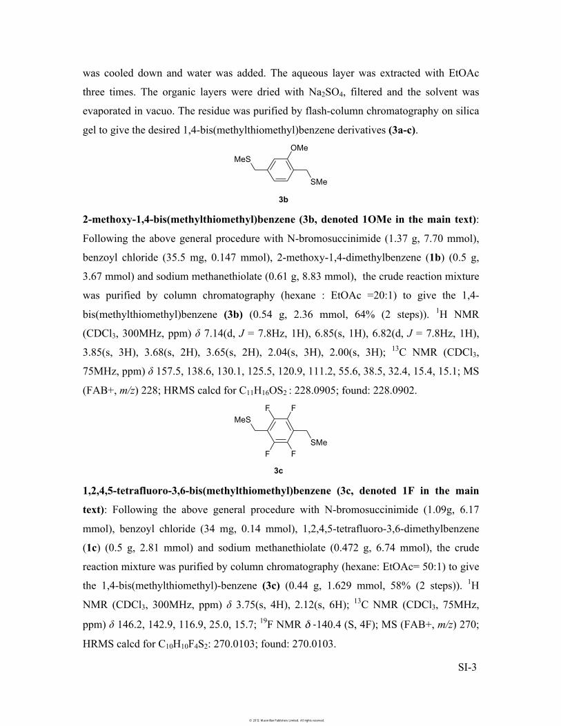
2-methoxy-1,4-bis(methylthiomethyl)benzene (3b, denoted 1OMe in the main text):
Following the above general procedure with N-bromosuccinimide (1.37 g, 7.70 mmol),
benzoyl chloride (35.5 mg, 0.147 mmol), 2-methoxy-1,4-dimethylbenzene (1b) (0.5 g,
3.67 mmol) and sodium methanethiolate (0.61 g, 8.83 mmol), the crude reaction mixture
was purified by column chromatography (hexane : EtOAc =20:1) to give the 1,4-
bis(methylthiomethyl)benzene (3b) (0.54 g, 2.36 mmol, 64% (2 steps)). 1H NMR
(CDCl3, 300MHz, ppm) � 7.14(d, J = 7.8Hz, 1H), 6.85(s, 1H), 6.82(d, J = 7.8Hz, 1H),
3.85(s, 3H), 3.68(s, 2H), 3.65(s, 2H), 2.04(s, 3H), 2.00(s, 3H); 13C NMR (CDCl3,
75MHz, ppm) � 157.5, 138.6, 130.1, 125.5, 120.9, 111.2, 55.6, 38.5, 32.4, 15.4, 15.1; MS
(FAB+, m/z) 228; HRMS calcd for C11H16OS2 : 228.0905; found: 228.0902.
1,2,4,5-tetrafluoro-3,6-bis(methylthiomethyl)benzene (3c, denoted 1F in the main
text): Following the above general procedure with N-bromosuccinimide (1.09g, 6.17
mmol), benzoyl chloride (34 mg, 0.14 mmol), 1,2,4,5-tetrafluoro-3,6-dimethylbenzene
(1c) (0.5 g, 2.81 mmol) and sodium methanethiolate (0.472 g, 6.74 mmol), the crude
reaction mixture was purified by column chromatography (hexane: EtOAc= 50:1) to give
the 1,4-bis(methylthiomethyl)-benzene (3c) (0.44 g, 1.629 mmol, 58% (2 steps)). 1H
NMR (CDCl3, 300MHz, ppm) � 3.75(s, 4H), 2.12(s, 6H); 13C NMR (CDCl3, 75MHz,
ppm) � 146.2, 142.9, 116.9, 25.0, 15.7; 19F NMR � �140.4 (S, 4F); MS (FAB+, m/z) 270;
HRMS calcd for C10H10F4S2: 270.0103; found: 270.0103.
3b
MeS
SMe
OMe
3c
MeS
SMe
F
FF
F
© 2012 Macmillan Publishers Limited. All rights reserved.

SI-4
Synthesis of various 2,11-dithia(3.3)paracyclophane derivatives
Preparation of various 2,11-dithia(3.3)paracyclophane derivatives: general protocol
(Scheme 2)
Potassium thio-acetate (2 equiv) was added to various 1,4-bis(bromomethyl)benzene
derivatives (2a-c) (1 equiv) in a mixture of CH2Cl2: MeOH (1:1 ratio). The mixture was
stirred at room temperature for 2h then filtered through a pad of celite. The solvent was
removed and the crude 1,4-bis(thio-acetate)benzene derivatives (4a-c) were used without
further purification in the next step. The crude 1,4-bis(thioacetate)benzene derivatives
(4a-c) (1 equiv), and the 1,4-bis(bromomethyl) benzene (2a-c) (1 equiv) were dissolved
in 10 ml of toluene and added, at room temperature, through a syringe pump (0.5 mL /
hour) to a solution of Cs2CO3 (2.2 equiv) in ethanol (100 mL). The solvent was removed
in vacuo. The residue was washed with water and extracted with CH2Cl2 three times. The
organic layers were dried with Na2SO4, filtered and the solvent was evaporated in vacuo.
The residue was purified by flash-column chromatography on silica gel (hexane: EtOAc=
50:1) to provide 2,11-dithia(3.3)paracyclophane derivatives (5a-c).
CH2Cl2, MeOH
KSAcBrBrBr Br
2a-cS S
KOH, EtOH, r.t.R
2a: R = H 5a: R = H
2b: R = OMe 5b:R = OMe
2c: R = 4F 5c: R = 4F
R
R
SAcAcS
R
4a: R = H
4b: R = OMe
4c: R = 4F
Scheme 2. Synthesis of various 2,11-dithia(3.3)paracyclophane derivatives.
R
X-ray structure of 5b
S S
5bOMe
MeO
© 2012 Macmillan Publishers Limited. All rights reserved.

SI-5
5, 14-dimethoxy-2- 11-dithia (3. 3) paracyclophane (5b, denoted 2OMe in the main
text):
Following the above general procedure with 2-methoxy-1,4-bis(thio-acetate)benzene (4b)
(100 mg, 0.340 mmol), 2-methoxy-1,4-bis(bromomethyl) benzene (2b) (96.7 mg, 0.340
mmol) and Cs2CO3 (243.7 mg, 0.748 mmol) in ethanol (100 mL), the residue was
purified by flash-column chromatography on silica gel (hexane: EtOAc=50:1) to provide
the thiocyclophane (5b) (58 mg, 0.175 mmol, 51%) which was confirmed by an X-ray
structure; 1H NMR (CDCl3, 300MHz, ppm) � 6.89(d, J = 7.7Hz, 2H), 6.55(s, 2H), 6.46(d,
J = 7.7Hz, 2H), 4.33(d, J = 10.8Hz, 2H), 3.87-3.72(m, 10H), 3.34(d, J = 10.8Hz, 2H); 13C
NMR (CDCl3, 75MHz, ppm) � 156.5, 130.5, 120.4, 111.7, 54.9, 38.0, 30.7; MS (FAB+,
m/z) 332; HRMS calcd for C18H20O2S2 : 332.0905; found: 332.0902.
5, 6, 8, 9, 14, 15, 17, 18-octafluoro-2, 11-dithia (3. 3) paracyclophane (5c, denoted 2F
in the main text): Following the above general procedure with 2, 3, 5, 6-tetrafluoro-1,4-
bis(thioacetate)benzene (4c) (122 mg, 0.374 mmol) and 2,3,5,6-tetrafluoro-1,4-
bis(bromomethyl)benzene (2c) (125.7 mg, 0.374 mmol), the residue was purified by
flash-column chromatography on silica gel (hexane: EtOAc= 20:1) to provide the
thiocyclophane (5c) (111 mg, 0.298 mmol, 80%) which was confirmed by an X-ray
structure; 1H NMR (CDCl3, 400MHz, ppm) � 3.96(s, 8H); 13C NMR (CDCl3, 75MHz,
ppm) � 144.7(d, JFC = 240 Hz), 115.1(m, CF), 24.9; 19F NMR � �140.4 (S, 8F); MS (EI+,
M+1) 416; HRMS calcd for C16H8F8S2 : 415.9940; found: 415.9913. The NMR spectra of
the compound (5c) are consistent with ones reported in the literature1.
S S
5cF
F
X-ray structure of 5c
F
FFF F
F
© 2012 Macmillan Publishers Limited. All rights reserved.

SI-6
General scheme for the synthesis of 2,7-bis(methylthiomethyl)-9H-fluorene 3d,
denoted 1Fl in the main text (Scheme 3).
Synthesis of 2,7-bis(bromomethyl)-9H-fluorene 2d (Scheme 3).
The fluorene (1d) (5g, 30.08 mM) was mixed with formaldehyde (3.6g, 120.30 mM),
phosphoric acid 96.9 mL) and HBr (48%, 9.4mL) in AcOH (12mL). The mixture was
stirred at room temperature for 6 hours then cooled down to 0 oC before HBr gas was
bubbled for 30 minutes. The reaction mixture was stirred at room temperature for 17h.
The precipitate was filtered out and heated under reflux in acetone for 1h. The white solid
was filtered and recrystallized in acetone to provide the desired 2,7-bis(bromomethyl)-
9H-fluorene 2d (6g, 23.8 mmol, 79%). 1H NMR (CDCl3, 300MHz, ppm) � 7.72(d, J =
8.1Hz, 2H), 7.57(s, 2H), 7.41(d, J = 8.1Hz, 2H), 4.60 (s, 4H), 3.89(s, 2H); MS (FAB+,
m/z) 352. The 1H NMR spectra of the compound (2d) is consistent with one reported in
the literature2.
Synthesis of 2,7-bis(methylthiomethyl)-9H-fluorene 3d (Scheme 3).
The 2,7-bis(bromomethyl)-9H-fluorene 2d (400 mg, 1.13 mM) was heated in dry DMF at
50 oC for 2h in the presence of sodium methanethiolate (191.1 mg, 2.72 mM). The
mixture was cooled down and water was added. The aqueous layer was extracted with
EtOAc three times. The organic layers were dried with Na2SO4, filtered and the solvent
was evaporated in vacuo. The residue was purified by flash-column chromatography on
silica gel to give the desired 2,7-bis(methylthiomethyl)-9H-fluorene 3d (241 mg, 0.85
mM, 75%). 1H NMR (CDCl3, 300MHz, ppm) � 7.69(d, J = 8.1Hz, 2H), 7.48(s, 2H),
7.27(d, J = 8.1Hz, 2H), 3.78 (s, 2H), 3.75 (s, 4H), 2.02 (s, 6H); MS (FAB+, m/z) 286.
HBr (48%), H3PO4
then, r.t., 17h1d 2d
NaSMe
DMF, rt - 50 oC, 2h
3d
Scheme 3. Synthesis of 2,7-bis(methylthiomethyl)-9H-fluorene 3d.
Br
Br
MeS
SMe
O
HH, ACOH
2. HBr, 30min
1.
© 2012 Macmillan Publishers Limited. All rights reserved.
SI-7
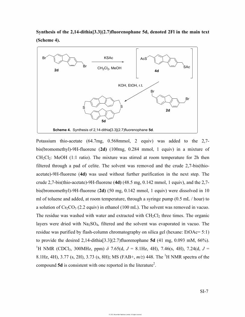
Synthesis of the 2,14-dithia[3.3](2.7)fluorenophane 5d, denoted 2Fl in the main text
(Scheme 4).
Potassium thio-acetate (64.7mg, 0.568mmol, 2 equiv) was added to the 2,7-
bis(bromomethyl)-9H-fluorene (2d) (100mg, 0.284 mmol, 1 equiv) in a mixture of
CH2Cl2: MeOH (1:1 ratio). The mixture was stirred at room temperature for 2h then
filtered through a pad of celite. The solvent was removed and the crude 2,7-bis(thio-
acetate)-9H-fluorene (4d) was used without further purification in the next step. The
crude 2,7-bis(thio-acetate)-9H-fluorene (4d) (48.5 mg, 0.142 mmol, 1 equiv), and the 2,7-
bis(bromomethyl)-9H-fluorene (2d) (50 mg, 0.142 mmol, 1 equiv) were dissolved in 10
ml of toluene and added, at room temperature, through a syringe pump (0.5 mL / hour) to
a solution of Cs2CO3 (2.2 equiv) in ethanol (100 mL). The solvent was removed in vacuo.
The residue was washed with water and extracted with CH2Cl2 three times. The organic
layers were dried with Na2SO4, filtered and the solvent was evaporated in vacuo. The
residue was purified by flash-column chromatography on silica gel (hexane: EtOAc= 5:1)
to provide the desired 2,14-dithia[3.3](2.7)fluorenophane 5d (41 mg, 0.093 mM, 66%). 1H NMR (CDCl3, 300MHz, ppm) � 7.65(d, J = 8.1Hz, 4H), 7.46(s, 4H), 7.24(d, J =
8.1Hz, 4H), 3.77 (s, 2H), 3.73 (s, 8H); MS (FAB+, m/z) 448. The 1H NMR spectra of the
compound 5d is consistent with one reported in the literature2.
CH2Cl2, MeOH
KSAc
KOH, EtOH, r.t.
4d
Scheme 4. Synthesis of 2,14-dithia[3.3](2.7)fluorenophane 5d.
2d
Br
Br
S S
5d
AcS
SAc2d
Br
Br
© 2012 Macmillan Publishers Limited. All rights reserved.

SI-8
Synthesis of 2,11-dithia(3.3)paracyclophane 7, denoted 1a in the main text (Scheme
5)
The 1,4-bis(bromomethyl) benzene (2a) (100mg, 0.381mmol, 1 equiv) and butane-1,4-
dithiol (6) (0.381mmol, 1 equiv) were dissolved in 10 ml of toluene and added, at 45 oC,
through a syringe pump (0.5 mL / hour) to a solution of Cs2CO3 (2.2 equiv) in DMF (50
mL). The mixture was diluted with water and extracted with CH2Cl2 three times. The
organic layers were dried with Na2SO4, filtered and the solvent was evaporated in vacuo.
The residue was purified by flash-column chromatography on silica gel (hexane: EtOAc=
50:1) to provide 2,11-dithia(3.3)paracyclophane (7) (56mg, 0.251, 66%). 1H NMR
(CDCl3, 400MHz, ppm) � 7.29(s, 4H), 3.77(s, 4H), 2.05(t, J = 7.2Hz, 4H), 0.74(d, J =
7.2Hz, 4H); 13C NMR (CDCl3, 125MHz, ppm) � 137.9, 130.3, 36.9, 30.59, 28.5; MS
(FAB+, m/z) 224; HRMS calcd for C18H20O2S2: 224.0693; found: 224.0687.
BrBr 6
Cs2CO3, DMF, 45 oC
2a 7
Scheme 5. Synthesis of the 2,11-dithia(3.3)paracyclophane 7.
S S
HSSH
© 2012 Macmillan Publishers Limited. All rights reserved.

SI-9
2. Table of Structures:
SI Table S1: Structure of all molecules investigated.
MeS
SMe1
1a
S S
S S
2
MeS
SMe
1OMe
S S
2OMe
OMe
MeO
OMe
MeS
SMe1F
S S
2F
F
F
F
FF
FF F
FF
F
F
MeS
1Fl
S
2Fl
SSMe
© 2012 Macmillan Publishers Limited. All rights reserved.
SI-10
3. Measurement and Data Analysis: We measured the molecular conductance of all molecules by repeatedly forming and
breaking Au point contacts in 1 mM 1,2,4 trichlorobenzene solution of the molecules
with a home-built, simplified STM3. A freshly cut gold wire (0.25 mm diameter,
99.999% purity, Alfa Aesar) was used as the tip, and UV/ozone cleaned Au substrate
(mica with 100 nm Au, 99.999% purity, Alfa Aesar) was used as the substrate. The STM
operates in ambient conditions at room temperature and the junctions were broken in a
dilute, 1mM, solution of target molecules in 1,2,4-trichlorobenzene (Sigma-Aldrich, 99%
purity). To ensure that each measurement started from a different initial atomic
configuration of the electrodes, the electrodes were pulled apart only after being brought
into contact with the Au surface, indicated by a conductance greater than a few G0. Prior
to adding a molecular solution between the tip and substrate, 1000 conductance traces
were first collected without molecules to ensure that there were no contaminations in the
STM set-up. Two-dimensional histograms were constructed from over 10000 measured
conductance trace for each compound considered. Conductance traces consists of
conductance data acquired every 25 µs, measured as a function of tip-sample
displacement at a constant 15 nm/s velocity. Since gold and molecular conductance
plateaus occur in random locations along the entire displacement axis (x-axis) within the
measured range, we first set the origin of our displacement axis at the point in the
conductance traces where the gold-gold contact breaks and the conductance drops below
G0. This well-defined position on the x-axis is determined individually for each trace
using an unbiased automated algorithm. For about 5% of the measured traces, this
position cannot be determined and these traces are not used for further analysis. Each
data point on the digitized conductance trace now has a conductance coordinate (along
the y-axis) and a position coordinate (along the x-axis). These data are binned using a
linear scale along the displacement axis and a log-scale along the conductance to generate
a 2D histogram.
© 2012 Macmillan Publishers Limited. All rights reserved.

SI-11
Additional Data:
SI Figure S1: 2D conductance histograms for junctions with molecules 1F (A) and 2F
(B) as a function of tip/substrate separation after breaking the Au-Au contact. C)
Conductance profile determined from the 2D histogram for 1F (green) and 2F (black) by
averaging over the region of width 0.1 nm shown by the vertical lines in (A) and (B).
SI Figure S2: 2D conductance histograms for junctions with molecules 1OMe (A) and
2OMe (B) as a function of tip/substrate separation after breaking the Au-Au contact. C)
Conductance profile determined from the 2D histogram for 1OMe (green) and 2OMe
(black) by averaging over the region of width 0.1 nm shown by the vertical lines in (A)
and (B).
© 2012 Macmillan Publishers Limited. All rights reserved.

SI-12
SI Figure S3: 2D conductance histograms for junctions with molecules 1Fl (A) and 2Fl
(B) as a function of tip/substrate separation after breaking the Au-Au contact. C)
Conductance profile determined from the 2D histogram for 1Fl (green) and 2Fl (black)
by averaging over the region of width 0.1 nm shown by the vertical lines in (A) and (B).
© 2012 Macmillan Publishers Limited. All rights reserved.
SI-13
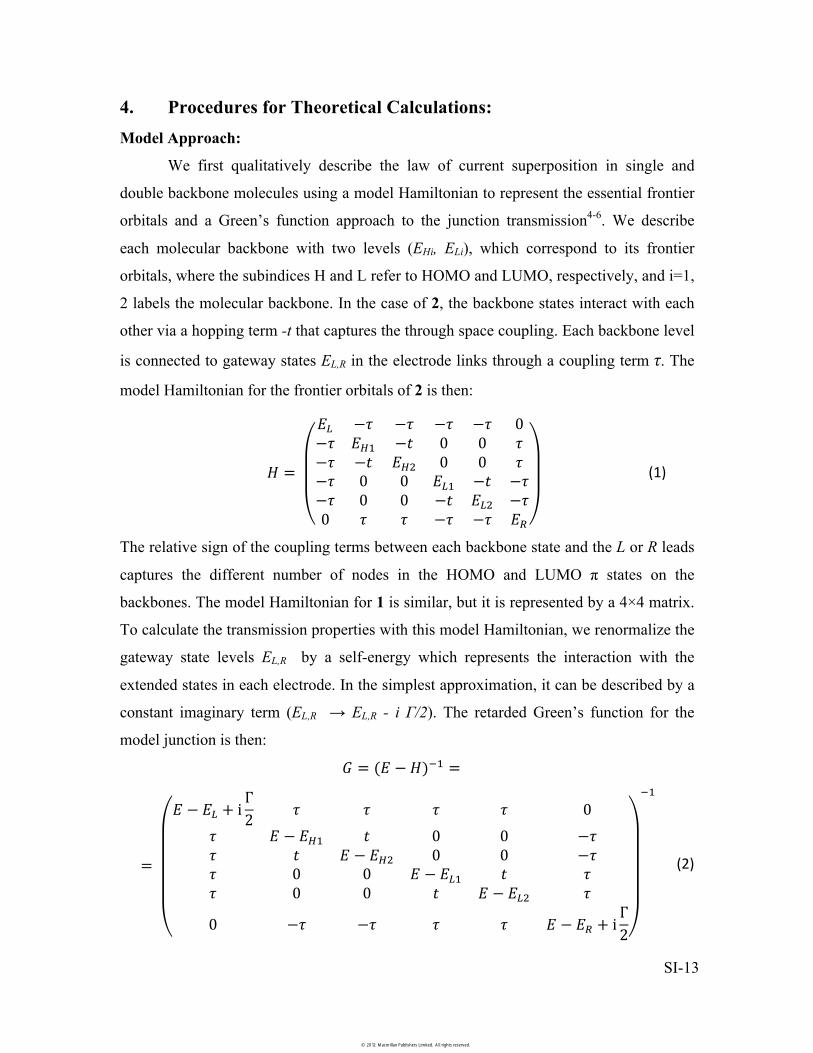
4. Procedures for Theoretical Calculations: Model Approach:
We first qualitatively describe the law of current superposition in single and
double backbone molecules using a model Hamiltonian to represent the essential frontier
orbitals and a Green’s function approach to the junction transmission4-6. We describe
each molecular backbone with two levels (EHi, ELi), which correspond to its frontier
orbitals, where the subindices H and L refer to HOMO and LUMO, respectively, and i=1,
2 labels the molecular backbone. In the case of 2, the backbone states interact with each
other via a hopping term -t that captures the through space coupling. Each backbone level
is connected to gateway states EL,R in the electrode links through a coupling term �. The
model Hamiltonian for the frontier orbitals of 2 is then:
� � �
�� �� �� �� �� ��� ��� �� � � ��� �� ��� � � ��� � � ��� �� ���� � � �� ��� ��� � � �� �� ��
� ���
The relative sign of the coupling terms between each backbone state and the L or R leads
captures the different number of nodes in the HOMO and LUMO � states on the
backbones. The model Hamiltonian for 1 is similar, but it is represented by a 4×4 matrix.
To calculate the transmission properties with this model Hamiltonian, we renormalize the
gateway state levels EL,R by a self-energy which represents the interaction with the
extended states in each electrode. In the simplest approximation, it can be described by a
constant imaginary term (EL,R � EL,R - i �/2). The retarded Green’s function for the
model junction is then:
� � �� � ���� �
� �
� � �� � ��� � � � � �
� � � ��� � � � ��� � � � ��� � � ��� � � � � ��� � �� � � � � � ��� �� �� �� � � � � �� � �
��
��
� �
���
© 2012 Macmillan Publishers Limited. All rights reserved.
SI-14
Finally, the transmission is given by T(E) = �2 |GLR(E)|2, where the indices on G refer to
the component of the matrix that couples to the left and right electrode respectively;
physically this represents the effective propagation from the left gateway state to the right
gateway state.
The transmission spectra in Fig. 1D for single- and double-backbone molecules
were generated by numerically solving equation (2) using the following parameters: EL,R
= -1eV, EH,= -2.4eV, ELi =+2.0eV, t = 0.3eV, � = 0.3eV, � = +2eV. For the double
backbone case, a slight asymmetry in the backbone states was introduced, EH1,L1 �
EH1,L1 – �, EH2,L2 � EH2,L2 + �, with � = 0.1eV. This small asymmetry gives rise to some
parasitic transmission through the antibonding backbone resonance, as described below.
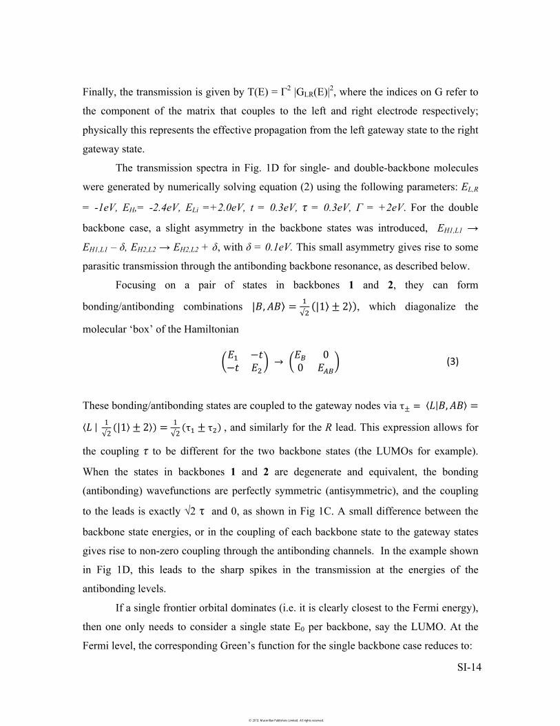
Focusing on a pair of states in backbones 1 and 2, they can form
bonding/antibonding combinations ����� � ��� �� � � , which diagonalize the
molecular ‘box’ of the Hamiltonian
These bonding/antibonding states are coupled to the gateway nodes via �� � � � ���� ��� � ��� �� � � � �
�� �� � �� �, and similarly for the R lead. This expression allows for
the coupling � to be different for the two backbone states (the LUMOs for example).
When the states in backbones 1 and 2 are degenerate and equivalent, the bonding
(antibonding) wavefunctions are perfectly symmetric (antisymmetric), and the coupling
to the leads is exactly �2 � and 0, as shown in Fig 1C. A small difference between the
backbone state energies, or in the coupling of each backbone state to the gateway states
gives rise to non-zero coupling through the antibonding channels. In the example shown
in Fig 1D, this leads to the sharp spikes in the transmission at the energies of the
antibonding levels.
If a single frontier orbital dominates (i.e. it is clearly closest to the Fermi energy),
then one only needs to consider a single state E0 per backbone, say the LUMO. At the
Fermi level, the corresponding Green’s function for the single backbone case reduces to:
�� ���� �� �� � �� �
� ��� ���
© 2012 Macmillan Publishers Limited. All rights reserved.

SI-15
������� � �
��
�� ��
�� �����
�
���
and the conductance is
� �� � � �
�� �� ������� �� ���
Transmission at the Fermi level for a double-backbone system with perfect
symmetry between the backbone levels can be calculated from equation (5) by realizing
that in this case, only the bonding state will contribute. Substituting the bonding level
energy and coupling Eb = E0 - |t| and ���� � � ��� for E0 and �, respectively, equation (5)
gives
� �� � �� �
�� �� � ������������
���
The ratio between the double- and the single- backbone systems is then:
������ �� � �
�� � ������� ��
�� � � ����������� � �
�� � ������� ��
�� � ���� � �������� ����
���
In the limit when E0 and � are large compared to 2� and t, this ratio approaches 4, the
ideal result. The model that includes both HOMO and LUMO, Eq. (1), also approaches 4
under the conditions described in the text. Both models give the same result as found by
a different argument previously 7.
Transmission calculations:
Structural relaxation calculations of the molecular junctions are carried out using
SIESTA8 with initial structures containing the molecule and Au tips in a 4x4 Au(111)
unit cell. The GGA (PBE) approximation is used for exchange-correlation9. Au atomic
orbitals are described using single-zeta polarized orbitals (with high cutoff radii for tip
© 2012 Macmillan Publishers Limited. All rights reserved.

SI-16
and surface atoms) and molecular atoms are described by double-zeta polarized orbitals.
Initially, the vertical distance is optimized by varying the electrode-electrode separation.
The structure containing 6 Au layers is then optimized until the forces on all molecule
and tip atoms are smaller than 0.02 eV/Å. We find a binding energy of ~0.9 eV per bond,
in agreement with previous work10. The C-C interbackbone distance is 3.5 Å.
Subsequent transmission calculations are carried out using TranSIESTA11 for
relaxed geometries built from these optimized structures by adding 3 extra Au layers on
each side of the supercell. The transport unit cell contains a total of Au 12 layers (Figure
S4).
SI Figure S4: Unit cell containing molecule 2 used in the transport calculations. White
atoms: H, grey: C, yellow: S, golden: Au.
The electronic structure is calculated using a 5x5 Monkhorst-Pack grid and a 250
Ry real-space cutoff. Transmission spectra are calculated with a 15x15 sampling of the
transverse Brillouin zone. The scattering states, the real part of which are presented in the
isosurface plots, are generated at the center of the Brillouin zone using the method of
Paulsson and Brandbyge12. The effect of the electrode tip structure was investigated by
© 2012 Macmillan Publishers Limited. All rights reserved.

SI-17
checking these results against optimized structures where each tip consists of a single Au
adatom. The conductance at the Fermi level differed by ~30% across the different
molecules, within the width of the experimental histograms (see Table SI1).
Figures S5A-C show the structure of the molecular junction of 1, 2 and 1c
structures. The ‘cut molecule’ 1c is obtained from the relaxed structure of 2 by removing
one backbone and saturating with H atoms. A comparison between the calculated
transmission spectra of 1 and 1c is shown in Figure S5D. Notice that both spectra exhibit
the same qualitative features, as molecules 1 and 1c have the same number of atoms and
structure, and differ only in their geometric arrangement at the junction.
SI Figure S5: Optimized junction geometries for the molecular structures of A) 1; B) 2
and; C) 1c. White atoms: H, grey: C, yellow: S, golden: Au. D) Calculated transmission
spectra of 1 (red) and 1c (green). The spectra of both single backbone molecules exhibit
the same qualitative features.
© 2012 Macmillan Publishers Limited. All rights reserved.

SI-18
Figure S6 shows the junction structure and transmission spectrum of the molecule
(1a) having a Benzene and a Butane backbone in parallel. Notice that, despite being a
double backbone molecule, its electronic properties are those of a single backbone
molecule, as it has only one conjugated backbone.
SI Figure S6: Optimized junction geometries for the molecular structures of A) 1a. White
atoms: H, grey: C, yellow: S, golden: Au. B) Calculated transmission spectra of 1a.
Notice the similarity in the junction structure and transmission spectrum with the single
backbone molecules 1c and 1 (Figure S5).
The paper shows how the conductance superposition law in single molecule
junctions results from the formation of bonding / antibonding pairs between states from
© 2012 Macmillan Publishers Limited. All rights reserved.

SI-19
each backbone. The main text illustrates this by focusing (Figure 3) on the orbitals that
have the largest influence on conductance. These are the state at 2.1 eV of 1c, and the
resulting bonding (1.9 eV) and antibonding (2.5 eV) states of 2. Figure S7 extends this
analysis to the resonances at -2.3 eV and 2.5 eV of 1, and the corresponding bonding /
antibonding pairs of 2.
SI Figure S7: Occupied (A) and unoccupied (B) scattering states of 1 (green), as well as
the corresponding bonding/antibonding states of 2 (black).
Figure S8 shows the molecular junction structure for the case of F and OMe
substituents and the corresponding transmission spectra. The same is shown in Figure S9
for molecules having Fluorene backbones.
© 2012 Macmillan Publishers Limited. All rights reserved.

SI-20
SI Figure S8: Optimized junction geometries for the molecular structures of A) 1F; B)
2F; C) 1OMe; D) 2OMe. White atoms: H, grey: C, yellow: S, pink: F, red: O, golden:
Au. Calculated transmission spectra of E) 1F (green) and 2F (black) and F) 1OMe
(green) and 2OMe (black). In both cases, the spectrum of the double backbone molecule
shows twice as many transmission peaks as that of the single backbone species.
© 2012 Macmillan Publishers Limited. All rights reserved.

SI-21
SI Figure S9: Optimized junction geometries for the molecular structures of A) 1Fl; B)
2Fl. White atoms: H, grey: C, yellow: S, golden: Au. C) Calculated transmission spectra
of 1Fl (green) and 2Fl (black).
© 2012 Macmillan Publishers Limited. All rights reserved.

SI-22
����������
�� ������
�� ������
��� ����
��� ������� ���� ��� �������
���������� �����������
1
2.7 × 10⁻³ G0 3.0�
4.3 × 10⁻³ G0 2.0
2 8.2 × 10⁻³ G0 8.6 × 10⁻³ G0
1F
3.5 × 10⁻³ G0 1.4�
6.4 × 10⁻³ G0 0.9
2F 4.8 × 10⁻³ G0 5.8 × 10⁻³ G0
1OMe
2.6 × 10⁻³ G0 2.4�
3.8 × 10⁻³ G0 1.4
2OMe 6.2 × 10⁻³ G0 5.3 × 10⁻³ G0
1Fl
7.2 × 10⁻⁴ G0 1.8�
1.1 × 10⁻³ G0 1.2
2Fl 1.3 × 10⁻³ G0 1.3 × 10⁻³ G0
1a 2.3 × 10⁻³ G0 �� 2.3 × 10⁻³ G0 ��
1c 2.5 × 10⁻³ G0 �� 2.6 × 10⁻³ G0 ��
SI Table S2: Calculated conductance (G0) at EF of the different single and double
backbone molecules with trimer and adatom tips.
We correct the DFT-based calculated conductance values of 1c, 1 and 2 by
considering the alignment errors in the position of the relevant frontier orbitals. We have
seen (Figure 3) that these are the occupied and empty molecular resonances closest to the
Fermi level: the resonance at -1.7 eV and the LUMO-derived peak. For each molecule,
we rigidly shift the position of these resonances by an amount which includes self-energy
corrections to the molecular level positions and screening effects at the interface. The
magnitude of the self-energy shift is calculated from differences in the total energy13 of
the neutral and charged molecule, ensuring that the excitation corresponds to the
appropriate molecular orbital (ie. localized on the S atom and on the LUMO,
respectively). The screening of these molecular excitations at the junction is described14
© 2012 Macmillan Publishers Limited. All rights reserved.

SI-23
by a classical image charge potential, assuming the charge to be localized on the S atom
and at the center of the benzene ring, respectively, and taking the image plane 1Å above
the Au(111) atomic plane15. We find the occupied resonance at -1.7 eV to be shifted only
slightly, while the position of the LUMO-derived peak has to be shifted up by ~0.7-0.8
eV. Specifically, the net shift, which includes both self-energy and image charge
contributions, for 1c, 1 and 2 is -0.2, 0.0 and -0.1 eV for the occupied resonance, and 0.8,
0.7 and 0.7 eV for the unoccupied one, respectively. By fitting the calculated
transmission spectra between these resonances to the sum of two lorentzians, we obtain
the change in the conductance ratio due to a shift in the resonance position. We find that,
within this two lorentzian approximation, the ratio G(2)/G(1c) is reduced by 7%, while
G(2)/G(1) is reduced by 20%, indicating that the conductance ratio is relatively
insensitive to the corrections to the DFT level alignment.
We calculate the conductance of single and double backbone molecules for
junctions stretched from their equilibrium electrode-electrode separations. The molecular
junctions were stretched from their equilibrium geometries by increasing the electrode-
electrode separation and relaxing all tip and molecular atoms. For 1 and 2, this was done
in steps of 0.3Å (SI Figure S10). We find that the conductance ratio G(2)/G(1) increases
as the junction is pulled since the molecular � system of 1 is better coupled to the
electrodes, making G(1) decrease more rapidly than G(2) as the electrode-electrode
distance increases. Similar calculations for F and OMe substituents and Fluorene
backbones when the junction was stretched by 1.2Å increase in the conductance ratios to
1.5, 2.6 and 2.8, respectively.
However, these substitutions introduce (antibonding) resonances in the double
backbone molecules in the energy window of the Au-S gateway states, reducing
transmission for energies near the Au-S end resonance (�-1.7 eV). Since low-bias
conductance is affected both by the bonding LUMO-derived peak as well as by this Au-S
end resonance, these additional peaks associated with substituents reduce the
transmission of the double backbone molecules with respect to 2 in the region below the
Fermi level. This makes the ratios G(2)/G(1) for substituents smaller than for the pair 1-2,
as measured experimentally.
© 2012 Macmillan Publishers Limited. All rights reserved.

SI-24
SI Figure S10. Ratio G(2)/G(1) between the calculated conductance at EF of double
backbone molecules and the corresponding single backbone analog, as a function of
vertical stretching from their respective electrode-electrode equilibrium separations, for
different molecular junctions. 1-2 backbones with trimer (adatom) tips: blue filled (open
squares. 1F-2F backbones with trimer tips: green triangles. 1OMe-2OMe backbones
with trimer tips: orange diamonds. 1Fl-2Fl backbones with trimer tips: black circles.
References:
1 Filler, R., Cantrell, G.L., Wolanin, D., & Naqvi, S.M., Synthesis of polyfluoroaryl[2.2]cyclophanes. J. Fluorine Chem. 30, 399-414 (1986).
2 Haenel, M.W., Irngartinger, H., & Krieger, C., Transannular Interaction in [M.N]Phanes .27. Models for Excimers and Exciplexes - [2.2]Phanes of Fluorene, 9-Fluorenone, and 9-Fluorenyl Anion. Chem. Ber. 118 (1), 144-162 (1985).
3 Venkataraman, L. et al., Single-Molecule Circuits with Well-Defined Molecular Conductance. Nano Lett. 6 (3), 458 - 462 (2006).
4 Nitzan, A., Electron transmission through molecules and molecular interfaces. Annual Review of Physical Chemistry 52, 681-750 (2001).
5 Datta, S., Quantum Transport - Atom to Transistor. (Cambridge University Press, 2005).
6 Hybertsen, M.S. et al., Amine-linked single-molecule circuits: systematic trends across molecular families. J. Phys.:Cond. Mat. 20 (37), 374115 (2008).
7 Magoga, M. & Joachim, C., Conductance of molecular wires connected or bonded in parallel. Phys. Rev. B 59 (24), 16011 (1999).
© 2012 Macmillan Publishers Limited. All rights reserved.

SI-25
8 Soler, J.M. et al., The SIESTA method for ab initio order-N materials simulation. J. Phys.:Cond. Mat. 14 (11), 2745-2779 (2002).
9 Perdew, J.P., Burke, K., & Ernzerhof, M., Generalized gradient approximation made simple. Phys. Rev. Lett. 77 (18), 3865-3868 (1996).
10 Park, Y.S. et al., Frustrated Rotations in Single-Molecule Junctions. J. Am. Chem. Soc. 131 (31), 10820-10821 (2009).
11 Brandbyge, M., Mozos, J.L., Ordejon, P., Taylor, J., & Stokbro, K., Density-functional method for nonequilibrium electron transport. Phys. Rev. B 65 (16), 165401 (2002).
12 Paulsson, M. & Brandbyge, M., Transmission eigenchannels from nonequilibrium Green's functions. Phys. Rev. B 76 (11), 115117 (2007).
13 Jaguar, Jaguar v7.8 (Schrodinger, L.L.C., New York, NY 2011). 14 Quek, S.Y. et al., Amine-gold linked single-molecule circuits: Experiment and
theory. Nano Lett. 7 (11), 3477-3482 (2007). 15 Smith, N.V., Chen, C.T., & Weinert, M., Distance of the Image Plane from Metal-
Surfaces. Phys. Rev. B 40 (11), 7565-7573 (1989).
© 2012 Macmillan Publishers Limited. All rights reserved.