Embed Size (px)
Citation preview

Summary Report „Geothermal Models at Supra-Regional Scale”
Title: Summary report “Geothermal Models at Supra-Regional Scale”
Authors: Goetzl Gregor & Zekiri Fatime (GBA) editor in cooperation with MFGI,
GEO-ZS, ŠGÚDŠ.
Austria: Goetzl Gregor, Hoyer Stefan, Zekiri Fatime
Hungary: Lenkey Laszlo
Slovakia: Švasta Jaromir
Slovenia: Rajver Dušan
Date: 30-SEPTEMBER-2012
Status: Final
Type: Text
Description: This report covers the elaboration on various geothermal models covering the
entire Transenergy project area at a scale of 1:500.000. The results are pre-
sented in terms of maps showing amongst others the Surface Heatflow Densi-
ty, subsurface temperatures at various depth levels, depths of 3 different tem-
perature levels as well as maps showing the geothermal potential.
Format: PDF
Language: En
Project: TRANSENERGY –Transboundary Geothermal Energy Resources of Slovenia,
Austria, Hungary and Slovakia.
Work package: WP5 Cross-border geoscientific models, task 5.2.4. Geothermal maps
covering the entire project area (supra-regional model)

2
Contents
Abstract ................................................................................................................................. 4
1 Introduction .................................................................................................................... 5
1.1 Definitions and Nomenclature ................................................................................. 5
1.2 Aims and deliverables ............................................................................................. 7
1.3 Project Area ............................................................................................................ 8
1.3.1 General overview ............................................................................................. 8
1.3.2 Austria .............................................................................................................11
1.3.3 Hungary (Lenkey L.) ........................................................................................15
1.3.4 Slovakia ..........................................................................................................20
1.3.5 Slovenia ..........................................................................................................27
2 Data background and workflow .....................................................................................30
2.1 Introduction ............................................................................................................30
2.2 Surface Heat Flow Density Map (HFD) ...................................................................31
2.3 Temperature and Depth Contour Maps ..................................................................32
2.4 Numerical Modelling (Background Heat Flow Density and Heat in Place) ..............32
2.4.1 Background Heat Flow Density .......................................................................32
2.4.2 Heat in Place ...................................................................................................33
3 Description of the applied methodologies and approaches ............................................34
3.1 Preparation of input data ........................................................................................34
3.1.1 Modelling of petrophysical data .......................................................................34
3.1.2 Thermal data processing .................................................................................41
3.2 1D modelling of the Surface Heat Flow Density (SHFD) .........................................42
3.3 Extrapolation of temperature within a borehole: ......................................................43
3.4 Estimation of Heat-In-Place and Identified Resources ............................................44
3.5 Geo-statistical interpolation ....................................................................................45
3.5.1 Interpolation methods for Surface Heat Flow Density ......................................45
3.5.2 Applied Interpolation methods for Temperature and Depth Maps ....................49
3.5.3 Interpolation methods for Heat-In-Place and Specific Identified Resources .....53
3.6 Estimation of background heat flow densities (Lenkey L. & Raáb D.) .....................53
3.6.1 Introduction .....................................................................................................53

3
3.6.2 Description of the chosen modelling approach ................................................54
4 Results ..........................................................................................................................59
4.1 Surface Heat Flow Density Map .............................................................................59
4.2 Temperature Map series ........................................................................................61
4.3 Contour map series of specific isotherms ...............................................................66
4.4 Geothermal Potential Map series ...........................................................................68
4.5 Distribution of Background Heat Flow Density (Lenkey L. & Raáb D.) ....................72
5 Summary and Conclusions ............................................................................................84
5.1 Surface Heat Flow Density and temperature maps.................................................84
5.2 Potential Map Series ..............................................................................................85
5.3 Background Heat Flow Density (Lenkey L. & Raáb D.) ..........................................87
5.4 Final Remark ..........................................................................................................88
References ...........................................................................................................................89
Enclosures ...........................................................................................................................95

4
Abstract
The aim of the Transenergy project is to enable the sustainable utilization of hydrogeother-
mal systems, based on the elaboration of interconnected geological, geothermal and hydro-
geological models.
The summary report “Geothermal models at a supra-regional scale” deals with the elabora-
tion and results of geothermal modelling at the scale of 1:500.000 covering the entire Tran-
senergy project area. One of the goals of the geothermal modelling at supra-regional scale
was to present an overview of the geothermal conditions for the entire project area in order to
enhance the awareness and understanding about existing resources. Furthermore geother-
mal boundary conditions could be determined for regional scale geothermal models within
the pilot areas. Based on that, the geothermal potentials and resources within the area could
be estimated to allow a sustainable (and balanced) utilization of the existing hydrogeothermal
resources.
The main input parameters for geothermal modelling were derived by re-processing data of
existing geothermal and hydrocarbon exploration wells and additional data obtained by la-
boratory measurements and literature research. The following parameters represent the
dominating influencing factors on the used modelling: surface heat flow density (HFD), rock
temperatures at different depths, depth contours of different temperature levels, natural geo-
thermal recharge, Specific Heat in Place (Specific HIP) and Specific Identified Resources.
The developed geothermal models were published in terms of maps at a scale of 1:500.000.
Additionally the 16 individual maps were grouped according to their aims (heat flow density,
temperature maps, contour maps, potential maps) stated above. They indicate prosperous
areas in terms of local to regional scaled geothermal anomalies (high HFD, Temperature or
Specific HIP values). Examples for these regions are the south-western part of the Transen-
ergy project area covering parts of the Styrian and Mura – Zala Basin and the central part of
the Danube Basin.
The elaborated potential maps provide a first perspective on available geothermal resources
and the actual degree of exploitation within the project area, irrespective to known or esti-
mated geothermal plays and reservoirs. However, the achieved results imply that only a very
small amount of the supposedly available geothermal resources is already utilized (<1%).
Therefore hydrogeothermal utilization may be able to play an important role in future energy
supply schemes of the Transenergy project area.

5
1 Introduction
The following report deals with the elaboration and outcomes of geothermal modelling at a
supra-regional scale 1:500.000 covering the entire Transenergy project area. These models
describe the natural geothermal conditions and resources with a clear emphasize on hydro-
geothermal utilization.
1.1 Definitions and Nomenclature
Table 1: Mathematic symbols
Symbol Parameter Unit Comment
q Heat Flow Density mW/m2
T Subsurface Temperature °C
T0 Temperature at Surface °C
z Depth m
m Thickness m
P Percentage %
∂T/∂z Temperature Gradient °C/m
A Area m2
λ Thermal Conductivity W/(m*K)
Cp Specific Heat Capacity J/(kg*K)
c relative proportion of rock type - within geological unit
ρ Density kg/m3
ɸ Porosity -
ΔH0 Heat in Place J see definition in Table 2
H1 Identified Resources J see definition in Table 2
R Recovery Factor - see definition in Table 2
S Data Class of Temperature -
Table 2: Definition of technical terms
Thermal Water Austria & Slovenia: Natural flowing groundwater with a constant
temperature above 20°C.
Hungary: Natural flowing groundwater with a constant tempera-
ture above 30°C.
Slovakia: Natural thermal water is groundwater, which is heated
by the action of heat in the earth's rock environment with minimal

6
temperature of water at 20 ° C. (Geological Act. 569/2007 Coll.).
Thermomineral water Slovenia: thermal water containing > 1000 mg/l of total dissolved
solids or 250 mg/l of free CO2.
Hydrogeothermal
Use
Utilization of naturally occurring thermal water for energetic or balneo-
logic purposes.
Heatflow Density
(HFD)
Amount of heat per time unit flowing across a unit area using the physi-
cal unit (W/m²) or (J/(sxm²).The governing transport process is consti-
tuted by either conductive heat transport and/or convective heat
transport or/and radiant heat transport.
Surface Heatflow
Density (SHFD)
Terrestrial HFD flowing to the surface of the Earth’s interior either by
conduction or convection. In practice the SHFD is calculated for an
observed section of a borehole or a well and reflects the geothermal
condition of the subsurface.
Heat in Place (HIP) Heat stored in a specified volume of subsurface porous rock and the
associated pore water using the physical unit (J) or (Wh during a speci-
fied time period).
Specific HIP Heat in Place referred to a unit area.
Specific Identified
Resources
Fraction of specific HIP regarding a Heat Recovery Factor. Note, that
not the entire heat amount stored in a defined rock volume can be re-
covered by technical measures.
Heat Recovery Fac-
tor
Ratio of recoverable heat to stored HIP. During Transenergy a constant
Heat Recovery Factor of 0.33 (equals to 33% of the stored heat techni-
cally recovered) has been assumed.
Table 3: Subscripts and Indices
Symbol Description
eff effective value
r rock
w water
m matrix
i i-th component
sp specific
inj injected
form formation
sh Shale/clay
ss sandstone

7
1.2 Aims and deliverables
One of the main subjects of Transenergy is the elaboration of geothermal models, which en-
able the sustainable utilization of hydrogeothermal systems. The models cover all aspects of
heat transfer due to conduction and advection (heat transport by externally driven forces, e.g.
gravitational or technical water flow) and intend to provide information about the initial and
actual geothermal conditions of existing thermal water reservoirs in terms of temperature
distributions and thermal balances. Naturally these models are closely linked to the also
elaborated geological- and hydrogeological models.
In general three different operating scales are applied in Transenergy:
i. Supra-regional scale 1:500.000 covering the entire project area
ii. Regional scale (1:100.000 up to 1:200.000) for selected pilot areas
iii. Local scale (<1:100.000) for selected geothermal reservoirs within the pilot areas.
Considering the different operating scales, the elaborated geothermal models certainly pur-
sue different goals. The actual report only treats the supra-regional scale geothermal models,
regional scale and local scale geothermal models will be discussed in subsequent, individual
reports.
Generally the following goals were defined for the supra-regional scale geothermal models:
Description of the overall geothermal conditions for the entire project area in order to
enhance the awareness and understanding about the existing resources.
Elaboration of geothermal boundary conditions for the regional scale geothermal
models at the pilot areas.
Estimation of existing geothermal potentials and resources at a supra-regional scale
in order to distinguish between prosperous and non-prosperous regions with respect
to hydrogeothermal utilization as well as to enable an overall hydrogeothermal bal-
ancing for the entire project area.
To achieve the already mentioned goals, the following thematic aspects have been investi-
gated for the entire project area:
Observed Surface Heat flow Density
Rock temperatures at different depth intervals and depth contours of different tem-
perature levels.
Natural geothermal recharge
Specific Heat in Place
Specific identified resources which equal the specific Heat in Place combined with an
invariant Heat Recovery Factor irrespective of hydrogeothermal reservoirs.
All achieved geothermal models have been published in terms of maps at a scale of
1:500.000 covering the entire project areas. The individual maps are grouped in different
map series, which picture the different aspects and aims mentioned above.

8
Table 4: Overview of achieved geothermal maps at a supra-regional scale of 1:500.000 covering the entire project area.
Thematic Aspect (Map Series) Title of Map and Content
Heat Flow Density Surface Heatflow Density Map
Temperature distribution in several
depth levels
Temperature at a depth of 1000m below
surface
Temperature at a depth of 2500m below
surface
Temperature at a depth of 5000m below
surface
Temperature at the depth of top Pre-
Tertiary basement
Contour Maps of different temperature
levels
Contour map of 50°C isotherm
Contour map of 100°C isotherm
Contour map of 150°C isotherm
Potential- and resource maps Heat in Place in sedimentary basin fillings
Heat in Place in top 50m at basement
Heat in Place in uppermost 5km of Earth’s
crust
Heat in Place in uppermost 7km of Earth’s
crust
Specific identified resources in sedimen-
tary basin fillings
Specific identified resources in top 50m at
basement
Specific identified resources in uppermost
5km of Earth’s crust
Specific identified resources in uppermost
7km of Earth’s crust
1.3 Project Area
The following chapter gives an introduction to the Transenergy project area with respect to
already existing knowledge about the geothermal conditions.
1.3.1 General overview
The Pannonian Basin and its adjacent areas cover the most prominent geothermal anoma-
lies of central Europe showing values of Surface Heat flow Densities up to 150mW/m², while
the global average is around 70mW/m². Although the major terrestrial Heat flux anomalies
are located at the eastern part of the Pannonian Basin, enhanced geothermal conditions are
also observed at its western part, which is covered by the Transenergy project area.

9
Figure 1: Overview of the geothermal condition at the Pannonian Basin regarding the distribution of Surface heat flow Density and lithospheric thickness.
10
The main reason for the enhanced geothermal conditions is understood as related litho-
spheric thinning, which is a consequence of plate tectonics (dilatation of the ALCAPA micro-
plate). As shown in Figure 1 the thickness of the lithosphere is gradually decreasing from
more than 120km to a minimum of less than 60km at the eastern part of the Pannonian Ba-
sin. In addition there are several local to regional scale heat flow anomalies superimposed to
the long scale variations of the terrestrial heat flow density. These anomalies are predomi-
nantly related to hydrodynamic systems, which lead to lowered geothermal conditions in re-
charge and descent areas, where “cold” meteoric waters are infiltrating, and effect positive
anomalies in the area of ascending and discharging “hot” thermal water. Further variations of
the terrestrial heat flow density are related to sedimentary and topographic effects, especially
at the margin areas of the western Pannonian Basin.
The geothermal conditions with respect to hydrogeothermal use in the project area have al-
ready been partly investigated in several previous studies. In general, these studies have to
be divided into:
i. High scale international geothermal atlases (e.g. Hurter & Haenel 2002, or Hurtig et al
1992).
ii. Transnational initiatives: DANREG between Austria, Slovakia and Hungary (1987 –
1997), Transthermal between Austria and Slovenia (2005 – 2008) and T-Jam be-
tween Slovenia and Hungary (2009 – 2011).
iii. National geothermal studies.
International geothermal atlases (i) are covering the entire project area but they generally
show a very low resolution at scales above 1:500.000. Furthermore it has to be pointed out,
that such geothermal maps depict the geothermal conditions at a very general and rudimen-
tary level.
The transnational activities (ii) mentioned above concentrated on the development of geo-
thermal maps with higher resolution (mostly scale 1:200.000), without covering the entire
project area (see also Figure). The DANREG project represents the first transnational activity
regarding hydrogeothermal conditions in the western Pannonian Basin with emphasis on the
so called Danube Basin sub-region. A major outcome of DANREG was achieved by provid-
ing a simplified map of maximum expected subsurface water temperatures above the crystal-
line basement of the Danube Basin (see also Kollmann 1997). During the period 2005 to
2008 the bilateral study Transthermal has been carried out between Austria and Slovenia,
which led to the elaboration of high quality hydrogeothermal potential maps outlining relevant
hydrogeothermal reservoirs of the Styrian Basin and the Slovenian Basin (see also Dom-
berger et a, 2008). A quantitative mapping of the available hydrogeothermal resources at the
trans-boundary Mura – Zala Basin has been achieved during the bilateral project T-Jam,
which has been conducted by Slovenia and Hungary and was accomplished in 2011 (for
more details visit http://en.t-jam.eu/project/).
Within the Transenergy project area a number of different scale national geothermal studies
without an Implementation of trans-boundary data are available. The previously accom-
plished national studies will partly be presented in the subsequent chapters of this report.

11
Transenergy is the first project offering harmonized datasets for the entire western Panno-
nian basin and its adjacent regions. However, the previously accomplished national and
transnational studies provide a crucial data basis for Transenergy project and should there-
fore not be neglected.
Figure 2: Overview of the project areas of previous transnational geothermal initiatives within the Transenergy project area, combined with the outlines of the different pilot areas of Tran-senergy.
1.3.2 Austria
In general a detailed geothermal atlas covering the entire area of Austria is still lacking.
However, a first comprehensive Heat flow Density map for Austria at a scale of 1:1.5 Mio
was published in 2007 (see also Figure 3) by Goetzl (2007). At large scale Austria offers
average geothermal conditions, which may vary significantly within the different regions.
The south-eastern parts of Austria clearly show enhanced heat flow densities due to the
geothermal influence of the adjacent Pannonian Basin. In this area maximum HFD values
of up to 120mW/m² were registered. Opposed to that moderate to low conditions can be
observed at the northern Alpine front (Northern Calcareous Alps) as a consequence of
crustal thickening combined with significant inflow of meteoric waters. In this area SHFD
values down to as less as 30mW/m² were measured. Due to lacking temperature meas-
urements the geothermal conditions within the Central Alpine Belt are not entirely
cleared. An existence of local to regional scale positive HFD anomalies caused by rapid

12
exhumation of deeply buried crustal segments is assumed for the area of the so called
Tauern Window.
Figure 3: Supra-regional Surface Heat flow Density map of Austria at the scale of 1:1.5 Mio, taken from Goetzl (2007).
The Austrian part of the supra-regional area covers the Vienna Basin, the Styrian Basin
and the western margin of the Pannonian Basin (see Figure 2). Several previous geo-
thermal studies were accomplished at the Austrian part of the Transenergy project area
because of previous and current (central and northern Vienna Basin) hydrocarbon explo-
ration.
The first regional scale geothermal investigations are based on temperature measure-
ments at artesian wells in eastern Styria and southern Burgenland (Zojer 1977, Zötl & Zo-
jer 1979). These studies resulted in temperature maps at a depth of 1000 meter below
surface and other maps showing the distribution of the geothermal gradient. The investi-
gated aquifers were limited to depths of approximately 200 meters below surface. There-
fore it can be supposed that the extrapolated geothermal conditions shown in these maps
have significantly been influenced by the conditions at the uppermost part of the under-
ground. During the bilateral Interreg IIIA Study Transthermal (2005 – 2008) the results of
the above mentioned studies have been re-evaluated using corrected BHT and DST da-
tasets from hydrocarbon exploration wells and temperature measurements at geothermal
wells in the Styrian Basin. These datasets were compiled to several geothermal maps in-
cluding a Heat flow Density map and additional map series showing the temperature dis-
tribution at several depth levels. Furthermore major geothermal reservoirs have been out-
lined and classified for a qualitative evaluation of available hydrogeothermal resources.
The elaborated so called Hydrogeothermal Potential Map series covers reservoirs in sed-
imentary basin fillings and basement rocks. An excerpt of these maps is shown in chapter

13
4. All maps are available at a scale of 1:200.000 and provide the distinction between
prosperous and non-prosperous regions for hydrogeothermal utilization. They have been
published by Goetzl et al 2008.
Figure 4: Overview on the Austrian part of the Transenergy project area with respect to selected previous studies

14
Figure 5: Geothermal potential map showing the outline of hydrogeothermal reservoirs in tertiary basin fillings (blue scattered lines) and at the pre-tertiary basement (red scattered lines) in the Styrian Basin and the Slovenian part of the Mura – Zala Basin. The yellow scattered
lines mark regions of intensive hydrogeothermal utilization. These results were gained at the bi-lateral Interreg IIIA study Transthermal (Goetzl et al, 2008).
Due to the large geothermal potential in the Vienna Basin several projects were executed at
the Geological Survey of Austria in the past 8 years. The scientific study THERMALP (2004 –
2012), financed by the Austrian Academy of Sciences – OEAW, investigated active hydrody-
namic systems at the southern Vienna Basin and pictured locally varying positive and nega-
tive geothermal anomalies. By applying 3D geological and numerical modelling several geo-
thermal maps showing the distribution of the Heat flow Density and subsurface temperatures
at different depths have been elaborated for this region (see also Figure 6). Furthermore a
regional scale geothermal and hydrothermal balance has been calculated for the most prom-
inent hydrodynamic1 reservoir at the southern Vienna Basin. They showed that the men-
tioned reservoir offers a utilizable heat content of approximately 50MWth2 for predominantly
balneological purposes which already is confronted with a degree of exploitation of almost
50% of the available resources.
The central and northern parts of the Vienna Basin have been investigated during the indus-
trial cooperative study OMV-Thermal (2008 – 2011). Based on water inflow observations at
hydrocarbon exploration wells in the Vienna Basin, hydrogeothermal resources for energetic
utilization in the range of 500MWth have been estimated for this region.
1 In this context hydrodynamic systems are defined as naturally circulating, actively recharged thermal
water reservoirs, which lead to local to regional scale geothermal anomalies. 2 Related to an ambient temperature of 10°C.

15
Figure 6: Surface Heat flow Density (SHFD) map for the southern and central Vienna Basin at a scale of 1:200.000 (taken from Goetzl et al, 2010). The regions with significantly lowered
SHFD values down to as less as 40mW/m² are related to crustal thickening at the Alpine thrust zone in combination with significant inflow of “cold” meteoric water. The gradually enhanced ge-othermal conditions toward the East are already related to the geothermal regime at the Panno-nian Basin. Toward the central and northern part of the Vienna Basin lowered geothermal condi-tions are assumed to be related to transient geothermal conditions caused by rapid sedimenta-tion. Locally confined positive heat flow anomalies are in turn linked to ascent paths and dis-charge areas of naturally circulating thermal water (hydrodynamic systems).
The results from the previous studies mentioned above, which were performed at the Geo-
logical Survey of Austria, were compiled and re-evaluated using recently acquired additional
data and improved processing algorithms in order to elaborate the supra-regional scale geo-
thermal maps presented in this report.
1.3.3 Hungary (Lenkey L.)
Due to intensive hydrocarbon exploration many boreholes and wells were drilled in the Little
Hungarian Plain and the Zala basin, in which BHTs, drill stem tests and other types of tem-
perature measurements were carried out. In the hilly parts of the Transenergy project area,
like e.g. the Transdanubian Central Range, temperature measurements in mining exploration
boreholes were conducted. Additionally the temperature of in- and outflow in thermal water

16
wells was recorded. These temperature data are stored in the Geothermal Database of Hun-
gary (Dövényi, 1994), which is continuously updated. The temperature data are corrected for
the transient effects of the drilling and represent the “true” formation temperature. The data-
base also contains the lithology of the boreholes and wells in order to estimate the thermal
conductivity of rocks. The thermal conductivity of the rocks is known from laboratory meas-
urements on core samples (Dövényi et al., 1983). Functions of the variation of the thermal
conductivity versus depth were established for neogene sands and shales (Dövényi and
Horváth, 1988).
In the area of the Transenergy project heat flow density was determined in five wells (Table
5). In these wells both temperature and thermal conductivity measurements were carried out.
In other boreholes and wells the heat flow density was estimated using thermal conductivity
values of Dövényi et al. (1983) and Dövényi and Horváth (1988), depending on the rock
types.
Table 5: Hungarian wells within the TE project area, where heat flow density determination was
carried out. For location of the wells see Figure 8. The expression No. of λ measurements
means thermal conductivity measurements on core samples from the well. References, a: Horváth et al., 1977, b: Horváth and Dövényi, 1987, c: Boldizsár, 1959, d: Horváth et al., 1989.
Name of well Short name No. of λ
measur.
HFD
(mW/m2)
Error Reference
Bárszentmihályfa-1 Bm-1 26 92 ± 20 % a
Bősárkány-1 Bős-1 17 83 ± 15 % b
Kerkáskápolna-1 Ker-1 12 90 ± 15 % b
Nagylengyel-62 Nl-62 12 84 ± 20 % c
Szombathely-II Sz-II 56 108 ± 15 % d
Heat flow density and temperature maps were elaborated for a larger area than the Transen-
ergy project area. A heat flow density map of Hungary is presented in the Atlas of Geother-
mal Resources in Europe (Dövényi et al., 2002), and in the assessment of geothermal ener-
gy resources in Hungary (Rezessy et al., 2005). The heat flow density in the Pannonian ba-
sin and surrounding area is shown in Figure 7 (Horváth et al., 2005), which represents an
updated version of the former heat flow density maps of the region (Dövényi, 1994, Lenkey
et al., 2002).
17
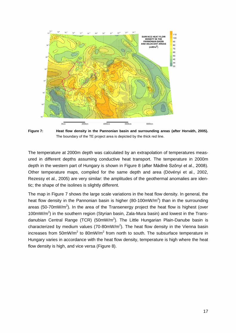
Figure 7: Heat flow density in the Pannonian basin and surrounding areas (after Horváth, 2005).
The boundary of the TE project area is depicted by the thick red line.
The temperature at 2000m depth was calculated by an extrapolation of temperatures meas-
ured in different depths assuming conductive heat transport. The temperature in 2000m
depth in the western part of Hungary is shown in Figure 8 (after Mádlné Szőnyi et al., 2008).
Other temperature maps, compiled for the same depth and area (Dövényi et al., 2002,
Rezessy et al., 2005) are very similar: the amplitudes of the geothermal anomalies are iden-
tic; the shape of the isolines is slightly different.
The map in Figure 7 shows the large scale variations in the heat flow density. In general, the
heat flow density in the Pannonian basin is higher (80-100mW/m2) than in the surrounding
areas (50-70mW/m2). In the area of the Transenergy project the heat flow is highest (over
100mW/m2) in the southern region (Styrian basin, Zala-Mura basin) and lowest in the Trans-
danubian Central Range (TCR) (50mW/m2). The Little Hungarian Plain-Danube basin is
characterized by medium values (70-80mW/m2). The heat flow density in the Vienna basin
increases from 50mW/m2 to 80mW/m2 from north to south. The subsurface temperature in
Hungary varies in accordance with the heat flow density, temperature is high where the heat
flow density is high, and vice versa (Figure 8).

18
Figure 8: Temperature at 2000m depth below surface in western part of Hungary. The boundary of
the Transenergy project area is depicted by the thick red line. Wells with temperature measure-ments are shown by black colour: D-1: Dabrony-1, BKSZ-I: Bakonyszűcs-I, BKCS-15: Ba-konycsernye-15. Wells with heat flow density determination are shown by red colour: Bm-1: Bá-rszentmihályfa-1, Bős-1: Bősárkány-1, Ker-1: Kerkáskápolna-1, Nl-62: Nagylengyel-62, Sz-II: Szombathely-II.
The low temperature and heat flow density values in the TCR are caused by groundwater
flow occurring in karstified Mesozoic carbonates. The area of the TCR is a recharge area,
where meteoric water precipitates. The groundwater seepages towards northwest and cools
the karstic aquifer in the basement of the Little Hungarian Plain (LHP) and the overlying neo-
gene sediments as it is observed in several wells (Figure 9). At the Rába line in the centre of
the LHP, which is the north-western boundary of the carbonatic rocks, the karstic flow turns
to northeast and southwest, and the discharge areas (the Komárom-Esztergom-Sturovo area
and the Hévíz area) are heated by the upwelling warm groundwater.

19
Figure 9: From Left to Right: Temperature in the Dabrony-1, Bakonyszűcs-1 and Bakonycsernye-15 wells. Black rectangles: measured temperature, red squares: corrected temperatures, green
line: temperature-depth curve calculated assuming heat conduction, right column: stratigraphy – the colour code is the following: yellow: Neogene, green: Cretaceous, purple: Triassic, dark pur-ple: Permian, blue: Palaeozoic.
Groundwater flow also occurs in the porous Upper Pannonian sediments. The heat flow den-
sity in the Szombathely-II well increases with depth from 90mW/m2 in the upper 1500m to
108mW/m2 below 1500m (Figure 10). The increase of heat flow density is interpreted by
groundwater flow in the Upper Pannonian sediments (Horváth et al., 1989). The sedimentary
layers are tilted towards east, the centre of the LHP, and the recharge area is located in a
distance of about 10.000-30.000m in the west where the Upper Pannonian sediments out-
crop to the surface.
Figure 10: Temperature and stratigraphy in the Szombathely-II well (Horváth et al., 1989). The expla-
nations see at Figure 9.
The LHP-Danube basin is characterized by smaller heat flow density values than the south-
ern regions in the TE project area. Solely based on observations it is difficult to say whether
the lower HFD values are due to groundwater flow in the carbonatic basement and in the
porous Upper Pannonian sediments, or due to reduced heat flow density coming from the

20
mantle. This question can only be answered by coupled modelling of groundwater flow and
heat transport. The results should be compared with results of pure thermal conduction mod-
els and observations.
1.3.4 Slovakia
The Slovak part of the supra-regional area includes the northern part of the Vienna Basin,
the northern part of the Danube Basin and a part of the Komarno-Sturovo area. In these re-
gions regional studies were already published, describing the geothermal conditions along
with calculations of geothermal water reserves, description of geothermal water circulation
and regimes. The main source for a general overview on pilot areas of the Transenergy pro-
ject is provided by the Atlas of Geothermal Energy of Slovakia (Franko, Remšík, Fendek,
(eds), 1995), which summarizes the existing knowledge from detailed studies until the end of
1994. The Atlas consists of detailed texts, maps, cross-sections and figures. This geothermal
atlas is based on temperature data from 376 boreholes, observed heat flow densities in 136
boreholes and hydrogeothermal data from 61 boreholes. The geothermal conditions at the
territory of Slovakia are represented in six different map series:
i. thematic geothermal map
ii. map of heat flow density at the surface
iii. map of heat flow density at the Moho-discontinuity
iv. geothermal maps of Slovakia
v. geothermal maps of delimited geothermal areas
vi. hydrogeothermal maps of delimited geothermal areas
All maps are accompanied by cross-sections, figures and well log profiles of geothermal
boreholes with outlines aquifers of geothermal plays at various geothermal areas. The text
part mainly points out the purpose of the Atlas as well as a description of the applied compi-
lation methods. Furthermore it comprises a general hydrogeothermal characterization of both
the entire territory of Slovakia as well as of individual geothermal areas at different regions. It
provides explanatory notes on technical aspects regarding the production of geothermal wa-
ter and possibilities for waste water disposal. The text is accompanied by tables and dia-
grams containing data about temperatures and heat flow density in boreholes, geothermal
installations and the chemical properties of geothermal waters. The Atlas is fundamental
knowledge for scientists, teachers, engineers, for governmental and industrial decision mak-
ers involved in exploring and exploiting geothermal energy and for the general public interest.
The Atlas is in bilingual Slovak – English edition.
In the following the geothermal areas situated at the Transenergy project area will be de-
scribed in detail:
(a) Vienna Basin
The pre-Tertiary relief (see Figure 11) of the Slovak part of the Vienna Basin is represented
by the slope of the Male Karpaty Mts. which in the west plunges to a depth of as much as
500m - 600m. It is dissected by numerous faults running NE-SW and W-E. The structure of
the pre-Neogene substratum is very complex. It has two essential elements - West Carpathi-

21
an and Eastern Alpine units. The two elements are separated by an abrupt change in the
earth's crust thickness. The geothermal characteristics are rather inhomogeneous, showing
areas with lowered and enhanced heat flow densities which seem to be trending roughly
along NW-SE axis. The lowered areas (heat flow density less than 45mW/m2) are located at
a south-western depression zone, whereas enhanced heat flow densities (exceeding
65mW/m2) have been observed at the Laksarska Nova Ves high block. The temperature re-
gime at existing hydrogeothermal reservoirs seems to be more homogeneous and shows an
antithetic trend compared to the distribution of terrestrial heat flow densities:
At the margin of the Male Karpaty temperature reaches less than 40°C and in the Rohoznik
area even less than 35°C. Temperature increases with distance from the mountains to more
than 45°C. In the Lab-Malacky block it exceeds 50°C while the highest reservoir tempera-
tures associated to naturally circulating water are observed in the Laksarska Nova Ves ele-
vation with a maximum of 55°C. The basin has no natural geothermal springs, therefore e
geothermal waters are tapped by two geothermal wells - RGL-1 at Laksarska Nova Ves and
RGL-2 at Sastin-Straze (Remšík et al, 1985 and 1989).
In addition, heated formation water has been observed in several hydrocarbon exploration
wells. These structures underlie the basin's neogene filling and are composed of several dif-
ferent tectonic nappes (predominantly Triassic formations at a higher stratigraphic position
than the Krizna nappe). Geothermal waters are bound to Triassic dolomites (mainly Upper
Triassic Hauptdolomite) of the Choc and higher nappes. Furthermore geothermal reservoirs
can be bound to Eggenburgian clastic sediments and to Karpatian sandstones and sands in
the southern part of the Vienna Basin (Lab - Malacky block). The hydrogeothermal system is
situated in a depth of 500 - 4500m and bears waters with a temperature of 40-140°C.

22
Figure 11: Map of the pre-Tertiary basement containing the temperature distribution and the depth of the pre-Tertiary basement (taken from Franko, Remšík, Fendek, eds, 1995).
(b) Danube Basin: Central depression
Central depression is fringed by the River Danube between Bratislava and Komarno in the
southwest, by the Male Karpaty in the northwest, by Dobra Voda fault (Ludince line) in the
northeast, and roughly by the River Nitra in the southeast. Several drill holes in the north-
western and south-eastern tracts of the depression have revealed that the Tertiary filling is
directly followed by crystalline rocks (crystalline schists, granitoids). From the hydrogeologi-
cal build-up of the Danube Basin it can be assumed that the Carpathian crystalline basement
of the Danube basin does not contain relevant geothermal aquifers. However, suitable aqui-
fers are bound to sands or sandstones of Pannonian, Pontian and Dacian age within the Ter-
tiary basin fillings.
The highest heat flow densities have been recorded in the middle of the depression (q > 85-
90mW/m2) and do not correspond to lower temperatures (T < 45°C) nor thermal gradients.
Whereas heat flow decreases towards the margins of the Danube basin, temperature in-
creases. This irregularity is caused by a cold water body, which is bound to the uppermost
hydro-geological unit showing a maximum thickness of 460m. The colder zone gradually per-
ishes downward and the temperature field corresponds to the heat flow. Badenian volcano-
clastics at depths of 5000 - 6000m may contain geothermal waters with aquifer temperature
exceeding 200°C. They can be utilized by applying reinjection for reasons of sustainability.
Because of its post-Sarmatian evolution, the Central depression has a bowl-like brachy-

23
synclinal shape (Priechodská, Z. - Vass, D. 1986). The hydrogeothermal characteristics of
the depression are summarized in Franko, Remšík, Fendek, eds, 1995. The upper boundary
of the geothermal water body is located at depths of 1000m below the surface and at the
bottom it is confined by a fairly impervious substratum - an aquitard (clays) which plunges
from the surrounding area towards the middle of the basin to a depth of up to 3400m below
surface.
This hydrogeothermal system is likely to have interlayer leakage, inter-granular permeability
and confined groundwater levels. It bears geothermal waters with registered temperatures
between 42°C and 92°C warm, which are bound to sands and sandstones of Dacian, Pontian
and Pannonian age. Figure 12 shows the temperatures and lithology at the depth of 5000m
below surface at the western part of Danube basin (Franko, Remšík, Fendek, eds, 1995).
Figure 12: Map of Danube basin – western part: Temperatures and lithology at the depth of 5000m below surface (taken from Franko, Remšík, Fendek, eds, 1995).

24
(c) Komarno block
The Komarno block extends between Komarno and Sturovo. It is fringed by the River Dan-
ube in the south and by the east – west striking Hurbanovo fault in the north, which is sepa-
rating this structure from the Veporic crystalline unit. The southern limit along the Danube is
also tectonically derived and therefore the Komarno block can be assumed to be a sunken
tract of the northern slope of the Gerecse and Pilis Mts. The surface of the pre-Tertiary sub-
stratum plunges towards the north from a depth of approximately 100m below surface near
the Danube (wells Sb-1 and FGŠ-1) to as deep as 3000m below surface near the before
mentioned Hurbanovo fault. The pre-Tertiary substratum of the Komarno block largely con-
sists of Triassic dolomites and limestones showing a maximum thickness of up to 1000m.
These dolomites are underlain by a very thick Lower Triassic shale formation. Palaeozoic
units were revealed by drilling in the north-western section of the Komarno block. These in-
clude Permian conglomerates, sandstones, graywackes and shales as well as Devonian
limestones and lydites. The Mesozoic and the underlying Palaeozoic formations of the Cen-
tral Hungarian Mountains were probably overthrusted onto the crystalline rocks of the Vepor-
ic crystalline unit, which is directly covered by Tertiary units northwards of the Hurbanovo
fault. However, the thrust plane sank along Hurbanovo fault and presumably reaches the
pre-Tertiary surface in the north-western tract of the Komarno block. It is assumed that at a
depth of 3000m below surface the Komarno block is dominated by Palaeozoic rocks and at
depths of 6000m below surface by the Veporic crystalline unit.
Geothermal waters are bound to Triassic limestones and dolomites. From a hydrogeothermal
point of view, the area is divided a high and marginal block (Remsik, A. - Franko, O. et aI.
1979; Franko, O. et. al. 1984; Remsik, O. et aI. 1992). Heat-flow densities suggest that the
high block shows fairly low and the marginal block medium conditions. This difference is as-
sumed to be caused by infiltrating cold karst waters.
The geothermal conditions at the high block are partly well known because of thermal
springs at Sturovo and Patince showing outflow temperatures of 39°C and 26°C. The Ko-
marno high block is confined by a 700 - 800m isobath of the Cretaceous carbonate substra-
tum or by tectonic lines running close to this isobath. The structure has a fast water circula-
tion and is considerably cooled (water temperature is varying from 20°C to 22°C at a depth of
600 to 800m below surface and varying between 24.5°C and 26.5°C at a depth of 1100 to
1300m below surface. At greater depths of 3000m below surface observed water tempera-
ture still remains at lowered levels of around 40°C. The hydraulic and thermal regime of geo-
thermal waters in the high block is directly controlled by variations in the water level of the
river Danube (Remsik, Franko et al 1979; Remsik, A. et al. 1992).
The Komarno high block is encircled by the marginal block in the west, north and east. The
latter contains ground waters whose temperature exceeds 40°C (whilst the highest so far
measured temperature is at a level of 68°C).
Figure 13 shows the pre-Tertiary basement in the western part of Danube basin and Komar-
no high and marginal block (Franko, Remšík, Fendek, eds, 1995).

25
Figure 13: Map of the pre-Tertiary basement in the western part of Danube basin and the Komarno high- and marginal blocks (taken from Franko, Remšík, Fendek, eds, 1995).
An additional summary of the geothermal conditions within the Slovakian part of the Tran-
senergy project area can be found at the Atlas of Geothermal Resources in Europe pub-
lished in 2002 (Hurter and Haenel, 2002). In this work the area of the Danube basin was de-
scribed by maps showing the distribution of temperature-, salinity-, thickness-, permeability-
and piezometric levels as well as showing resources of geothermal regimes of Pontian and
Pannonian to Pontian age (see also Figure 14 and Figure 15).

26
Figure 14: Example map of the geothermal resources calculated in Pannonian-Pontian horizons in Danube Basin, compiled for Atlas of Geothermal Resources in Europe 2002 (taken from Hurter and Haenel, 2002).
Figure 15: Example map of the temperature and salinity in Pannonian-Pontian horizon in the Dan-ube Basin compiled for Atlas of Geothermal Resources in Europe, 2002 (taken from Hur-ter and Haenel, 2002).

27
1.3.5 Slovenia
The Slovenian part of the supra-regional area consists of the Mura-Zala basin in north-
eastern Slovenia, which is situated in the south-western corner of the Pannonian basin. Due
to the reduced crustal thickness (less than 30km east of Maribor), this area comprehends the
greatest geothermal potential in Slovenia with respect to temperatures and heat flow density.
Many users have already started direct heat use of geothermal energy in this region 2 - 3
decades ago. Recently new projects in Murska Sobota and Renkovci have been established.
The planning of thermal water utilization in spas and greenhouses led to some local studies
(in Murska Sobota, Moravske Toplice, Ptuj, Lendava). Temperature and surface heat flow
density maps were compiled for the whole country in the previous studies, although the main
focus is set on north-eastern Slovenia.
Figure 16 to Figure 18 show some of the already existing maps. These maps can also be
found in the publication by Rajver & Ravnik (2002). In large parts of the Mura-Zala basin (ex-
cept the Goričko region), east of the line Maribor-Ptuj, the geothermal potential is used by
spas, thermal resorts and greenhouses.
Figure 16: Heat Flow Density Map of Slovenia (Ravnik et al., 1995).

28
Figure 17: Temperature distribution at a depth of 1000m (Ravnik et al., 1995)
Figure 18: Geothermal resources and potential areas in Slovenia (Rajver et al., 2002)
The existing maps of heat flow density and temperature cover the whole country. However,
they are more detailed and of better quality in north-eastern Slovenia due to a higher concen-
tration of deep boreholes. The investigation area is characterized by increased geothermal
gradients as wells as increasing surface heat flow density (SHFD).
At a depth of 1000m below surface, high temperature anomalies are discernible from Lenart
to Moravske Toplice and around Lendava (expected formation temperature from 60°C to

29
70°C). Elsewhere in north-eastern Slovenia the subsurface temperatures are just a little
above average (44°C to 55°C) at the above mentioned depth. The surface heat flow density
reaches more than 100mW/m2 eastwards of the town Maribor with an exception of the Ptuj
area, probably due to lacking measurements and evaluation. The map showing the geother-
mal resources and potential areas (Figure 18) was prepared for the “Atlas of Geothermal
Resources in Europe” (Hurter and Haenel, 2002). It illustrates the calculated Identified Re-
sources for north-eastern Slovenia, where the Tertiary Mura formation represents the most
promising reservoir.
The increased HFD values were determined especially on the Murska Sobota High between
Lenart and Moravske Toplice and are attributed to the convection zones in the pre-Tertiary
basement rocks. This is already confirmed at the exploration-production well in Benedikt,
terminating at a depth of almost 1900m in the metamorphic, highly fractured dolomitic mar-
bles with thermal water convection. This leads to an increased temperature gradient within
the overlying tertiary beds and consequently to high HFD values (around 145mW/m2). A simi-
lar situation with convection zones in the metamorphic pre-Tertiary rocks can be expected in
the northeast, at Murska Sobota and Moravske Toplice at depths of about 1100 – 1500m as
well as at Lendava – here at much greater depths (around 4000m). These assumptions
could not be proven yet.
Figure 19: From top left to bottom right: temperature distribution maps in depths of 250, 500, 1000, 1500, 2000, 3000, 4000m and a surface heat flow density map (Rajver et al., 2008; Rajver &
Goetzl, 2007)
Within the INTERREG IIIA project “Transthermal”, several geothermal maps of the project
area have been created (Figure 19). For the Slovenian part of the project area geothermal

30
data from about 300 boreholes have been analysed. Temperature maps indirectly show the
geothermal gradients in the Tertiary sediments. Those are increased almost everywhere in
north-eastern Slovenia (east of Maribor), especially between Lenart and Moravske Toplice,
and reach values of up to 80mK/m on the Murska Sobota high. The geothermal gradient is,
however, more reduced in the pre-Tertiary bedrock (carbonatic as well as metamorphic).
The HFD map also shows remarkably differing values in the north-eastern part (Mura-Zala
basin) and in the rest of northern Slovenia, i.e. west of Maribor. For the entire Slovenian part
of the Transthermal project area the average HFD value (± s.d.) is about 87 ± 34mW/m2
(conclusion from data of 50 wells). However, for the Pannonian (Mura-Zala) part of the basin,
the average HFD value (derived from 26 wells) is higher about 114 ± 22mW/m2. This is a
consequence of different lithospheric conditions in both areas (Goetzl & Lapanje (eds.) et al.,
2008). Considering, as an example, singly the map of temperatures in a depth of 2000m,
they are higher than 84°C practically everywhere east of the Maribor – Ptuj line. Here, the
Benedikt anomaly is not discernible anymore - the thermal circulation causes high geother-
mal gradients only in the sedimentary cover. In Slovenia, the highest temperatures (above
100°C) at that certain depth are found at Veržej, across Murska Sobota towards Moravske
Toplice and northeast from there, as well as in the wider Lendava area (Goetzl & Lapanje
(eds.) et al., 2008). Elsewhere in north-eastern Slovenia, elevated temperatures at different
depths appear also in the other smaller areas, i.e. SE of Lendava, between Maribor and
Radenci, and along the border with Hungary. Further anomaly zones can be expected (for
example north of Pečarovci and Šalovci), but have not yet been detected.
Advective heat transfer due to deep water circulation is capable of provoking locally confined
anomalies to the geothermal regime down to depths of 1, 5 to 3km below the surface, de-
pending on the existence of hydraulically conductive layers or fault-systems within crystalline
bedrocks. The overall geothermal regime is in turn mainly controlled by the conductive heat
exchange depending on the regional crustal thickness, leading to significant changes of geo-
thermal conditions between the Mura-Zala basin and the other areas of northern Slovenia
(Goetzl & Lapanje (eds.) et al., 2008).
2 Data background and workflow
2.1 Introduction
The geothermal regime of the supra-regional model is represented by means of temperature
maps for several depths as well as by a surface heat flow density map. By using continuous
thermal logs, bottom-hole-temperature (BHT) and drill-stem-test (DST) data obtained from
wells, it is possible to estimate the geothermal regime. In addition to the in situ-data, outflow-
ing water temperatures were included in the thermal processing. Because of the different
data background in each country, the project partners did not work with the same types of
data. In Austria, corrected BHT- and DST-data were used. In Slovenia mostly data from con-
tinuous thermal logs have been interpreted, as they are available in a very good quality. In
Hungary, outflow temperatures were accessible in addition to BHT- and DST-data. The ap-

31
plied Slovakian datasets were derived from the Slovakian Geothermal Atlas (Franko, Remšik
& Fendek, 1995).
Apart from required temperature data, parameters such as thermal conductivity and po-
rosity had to be known for a determination of heat flow density. These data come from lit-
erature as well as old and new core measurements (see chapter 3.1.1).
In general the mapping of the geothermal regime is based on the following workflow:
1. Thermal Data Processing
2. Modelling of petrophysical data
3. Estimation of Heat Flow Density (in a borehole)
4. Estimation of Temperatures in various depths:
a. 1000 m.b.s
b. 2500 m.b.s
c. 5000 m.b.s
d. Top of pre-Tertiary basement
5. Estimation of Depth of different isothermal surfaces
a. 50°C
b. 100°C
c. 150°C
6. Estimation of Specific Heat In Place and Specific Identified Resources
7. Interpolation and Visualization of Data from 4.-6
8. Modelling of the basal (background heat flow density)
2.2 Surface Heat Flow Density Map (HFD)
Overall, thermal data from 1243 wells were processed for the elaboration of the map. It
was necessary to exclude 30 HFD values, because they were either unrealistically high
(up to values of 1400mW/m2) or had no specified location. The applied cut-off value for
filtering of input data was set to 170mW/m2. Furthermore four artificial datum points had
to be added to the dataset in order to enhance the density of input data for interpolation.
The majority of the HFD data was gathered in Hungary (731 values) and Austria (418
values). The remaining data was provided by Slovakia (57) and Slovenia (37).
Since the thermal logs in Slovenia (due to long shutdown times) are of good quality, the
measured temperatures can be assumed as true formation temperature. Despite this, the
Hungarian datasets have been divided into 9 different classes of quality, where >1<
equals a very good and >9< an insufficient data quality. Furthermore the classification of
the quality of Austrian data is based on differentiation between DST- and corrected BHT-
values. In general temperature measurements during drill-stem-tests are more reliable
because of the long shutdown time.

32
2.3 Temperature and Depth Contour Maps
Temperature Maps:
The compilation of temperature maps was performed at the depths of 1000m, 2500m and
5000m below surface (m.b.s).
The map at 1000 m.b.s was created using 6220 temperature values. The reason for this
huge amount of values is the fact that the Slovakian partner has provided a GIS shape
file with temperature values (as point information) extracted from contour lines of existing
geothermal maps in addition to data from individual wells. Extracted points from contour
lines were treated as data from wells in order to enhance the density of input data. The
same procedure was applied for the other maps. The cut-off value for data filtering was
set to 125°C. Only five values in total had to be excluded since they were unrealistically
high (between 200 – 450°C).
The temperature map at a depth level of 2500 m.b.s. is basing on 6523 temperature val-
ues. Once again around 75 % of the available input data resulted from the Slovakian
shape files. Again, an exclusion of data was unavoidable. The upper cut-off value was set
to 250°C and the lower one to 20°C. Therefore, seven unrealistic temperature values with
of up to 1000°C and lows of around 15°C had to be filtered out.
The temperature map at 5000 m.b.s was created using 6294 temperature values. The
largest amount of these values originates again from the Slovakian dataset. This time, no
exclusion of data was necessary, but nine artificial wells had to be added. This was es-
sential for stabilization purposes of the interpolation at the border of the supra-regional
model.
The temperature map at the top of the pre-Tertiary basement was compiled using 1850
temperature values. At locations where the basement is outcropping at the surface invar-
iant temperature values of 10°C, which reflect the annual surface temperature at a first
approach, were used for interpolation.
Depth Contour Maps of different isothermal surfaces:
Three Depth Contour maps of the 50°C, 100°C and 150°C isothermal surface were
produced by 3D interpolation of temperature data from the temperature maps described
above. The 3D interpolation was applied by using the numerical modelling software
FEFLOW™.
2.4 Numerical Modelling (Background Heat Flow Density and Heat in Place)
2.4.1 Background Heat Flow Density
The dominant way of heat transport in the continental lithosphere is conduction. However,
groundwater flow occurring in porous and fractured rocks in the upper part of the crust can
modify the temperature field by convective heat transport. Depending on the flux of the
groundwater flow the redistribution of heat can be significant resulting in strong temperature
and heat flow density anomalies. Heat conduction can also result in thermal anomalies due

33
to variation of mantle heat flow density, heat production and thermal conductivity of rocks.
Those thermal anomalies which cannot be explained by conduction are very likely caused by
groundwater flow.
The background heat flow density is the heat flow density in sufficiently large depth, where
the effect of near surface convective heat transport can be neglected. It is calculated assum-
ing pure conductive heat transport and radiogenic heat production at the Earth’s Crust.
Based on project related datasets of (i) Surface Heat Flow Densities, (ii) interpolated subsur-
face temperatures and (iii) thermal rock parameters (see also Table) the background heat
flow density was modelled for the entire lithosphere beneath the Transenergy project area.
For that purpose assumptions for the build-up of the lithosphere were taken from literature
sources and previous studies. The modelling was performed by using the numerical software
package Comsol Multiphysics™. Further details can be found at chapter 3.
Comparing the distribution of the background heat flow with the observed surface heat flow
allows outlining and characterizing geothermal anomalies driven by convection of thermal
water.
2.4.2 Heat in Place
The parameters Specific Heat in Place and Specific Identified Resources represent the exist-
ing geothermal potential assuming that 100 % (Specific Heat in Place) or 33 % (Specific
Identified Resources) of the available heat content at the subsurface can be extracted by
cooling to a defined lower temperature level (reference temperature). These parameters limit
the theoretically utilizable geothermal heat in a first approach ignoring the hydrogeological
build-up of the subsurface. These two parameters can be estimated if the distribution of the
following parameters in the subsurface is known: (i) specific heat capacity, (ii) bulk density,
(iii) total porosity, and (iv) thickness of the investigated rock volume and (v) subsurface tem-
perature.
The compilation of the parameters Specific Heat in Place and Specific Identified Resources
was performed for four different cases:
i. in the Neogene sediments
ii. in the 50m upper part of pre-tertiary basement
iii. until a depth of 5km
iv. until a depth of 7km
The petrophysical input data (parameter: i to iii) were obtained from modelling and calibration
by measurements on rock samples at the Austrian part of the supra-regional model (see also
Table). At the other parts of the supra-regional area (Hungary, Slovakia and Slovenia) a
simplified approach was applied by correlating petrophysical properties to the stratigraphical
build-up, which consists of alternating clay and sand layers. The values of these parameters
were obtained from literature and laboratory measurements (see chapter 3.1.1). For more
details see also chapter 3.1.1.

34
The total thickness of the Neogene Sediments was derived from the geological model of the
supra-regional area, whereas the thickness of the individual sedimentary horizons is based
on literature research.
Assuming linear increase of temperature between the surface and depths of 1000m, 2500m
and 5000m below surface, the temperature for a certain depth could be calculated. Below
5000m the temperature was extrapolated with the last gradient (between 2500 and 5000m).
The surface temperature was assumed to be uniform (10°C). Furthermore, the temperature
of re-injected water has to be known when calculating the Specific Identified Resources. The
value was set to 25°C, so that a comparison of the Specific Identified Resources with previ-
ous studies (Franko et al., 1995, Hurter and Haenel, 2002) was possible.
3 Description of the applied methodologies and approaches
The following chapter treats the applied methodologies in order to elaborate the models and
maps covering the entire project area. It intends to give a comprehensive understanding to
the chosen approaches for:
the preparation of petrophysical and thermal input data
the geostatistical interpolation in order to elaborate the several maps
the calculation of several geothermal potentials
the applied 3D modelling for the estimation of the background heat flow density
This in turn shall enable a possible future adaption and update of the achieved results.
3.1 Preparation of input data
In general the applied input data are represented by petrophysical parameters and borehole
related thermal data. Both datasets are related to different scales and approaches, which will
be described in the subsequent subchapters.
3.1.1 Modelling of petrophysical data
In general heat transport is governed by the following material parameters:
a. Thermal conductivity
b. Specific heat capacity
c. Bulk porosity and density
d. Effective porosity
e. Radiogenic heat production
These formation characteristics were obtained for individual rock types from previous studies
as well as from literature and exploration data. Since only values for individual rock types are
known, generalized models for the pre-specified geological units at supra-regional scale (see
Summary report of geological models, http://transenergy-eu.geologie.ac.at/) had to be de-
fined.

35
As in Austria comprehensive laboratory measurements of thermal rock properties just com-
menced a couple of years ago and synthetic models of the geological units appearing in the
subsurface of the Transenergy project area had to be calculated by means of weighted aver-
aging according to the appearance of different rock types. The petrophysical parameters of
individual rock types themselves had been taken from literature (e.g. Schoen, 1983). After-
wards the achieved petrophysical models were calibrated and evaluated by measured data
gained from drilling-core analyses. The frequency of the individual rock types obtaining within
a geological unit was used as a weighting factor for estimation of the material parameters.
For the remaining parts of the supra-regional area, a simplified correlation between petro-
physical parameters and the stratigraphical build-up of the Tertiary basin fillings was con-
ducted. This correlation is based on the alternation of shale and sand layers. As the variation
of thermal properties at consolidated basement is much lower than in the basin fillings due to
reduced porosity, simple models of weighted averages have been applied on the hard rocks
of the pre-Tertiary basement.
a. Thermal conductivity:
As this material parameter provides information about the ability to transport heat, it is im-
portant for the interpretation and prediction of formation temperature. The thermal conductivi-
ty for estimation of the surface heat flow density was determined by following approaches:
In Austria, the mean thermal solid matrix conductivity for a geological unit was predicted in a
first approach from the lithological composition of the layer:
∏ ∑ 3-1
The effective thermal conductivity represents the true formation characteristic, taking into
account fluid-filled pore space and ambient temperature. According to Beck (1976), the effec-
tive parameter can be calculated by following equation:
∏
3-2
Furthermore, the parameter is affected by temperature. Empirical studies indicate that the
effective thermal conductivity at a temperature around 200 °C is reduced by 30 % compared
to the value at room temperature. For the estimation of the surface heat flow density a ther-
mal correction, based on Sass et al. (1992), was unavoidable:
(
) 3-3
The hypothetical thermal conductivity of the individual rock type at 0 °C [λ0=λ(0)] can be de-
rived from following equation:
[ (
)] 3-4

36
Table 6: Thermal parameters of rocks used for the calculation of Specific HIP and Specific Identi-fied Resources (see chapter 3.4). Data of the Vienna and Styrian basin are from laboratory
measurements made in the framework of TE project. Specific heats of clay and sand in other areas are from Kappelmeyer and Haenel (1974), bulk densities are from Szalay (1982).
Vienna basin
Specific heat
(J/kg.K)
Bulk density
(kg/m3)
Porosity
(%)
Horizon mean min max mean min max mean min max
Quaternary 758 758 758 1800 1800 1800 30 30 30
Upper Pannonian 782 754 807 1943 1900 2200 24 21 25
Lower Pannonian 782 754 807 1943 1900 2200 24 21 25
Sarmatian 767 763 769 1920 1900 1957 25 24 25
Badenian 1002 886 1176 2313 1963 2730 18 7 26
Lower Miocene 1062 957 1161 2450 2127 2680 13 6 20
pre-Tertiary base-
ment
958 894 1121 2621 2200 2897 5 0 20
Styrian basin
Specific heat
(J/kg.K)
Bulk density (kg/m3) Porosity
(%)
Horizon mean min max mean min max mean min max
Quaternary n.d. n.d. n.d.
Upper Pannonian 787 2362 2189 2552 19 14 29
Lower Pannonian 787 2362 2189 2552 19 14 29
Sarmatian 774 774 774 n.d. 20 20 20
Badenian 803 769 829 2412 2270 2476 12 4 17
Lower Miocene 851 800 888 2546 2357 2728 6 5 8
pre-Tertiary base-
ment
762 710 853 2709 2644 2799 3 0.3 18
Other areas (HU: Little Hungarian Plain, SK: Danube basin, SL: Drava basin)
Specific heat Bulk density (kg/m3)

37
(J/kg.K)
Clay 950 2710
Sand 920 2620
pre-Tertiary base-
ment
960 2620
Table 7: Thermal parameters of rocks used for the calculation of Background Heat Flow Density (see chapter 3.6).
Vienna Basin
λ
(W/m.K)
A
(10-6 W/m3)
c
(J/kg.K)
(kg/m3)
Horizon mean min max mean min max
Quaternary 3 3 3 n.d. 1282 2300
Upper Pannonian 3.1 2.8 4 1.3 1.3 1.3 1282 2300
Lower Pannonian 3.1 2.8 4 1.3 1.3 1.3 1282 2300
Sarmatian 3.2 3 3.3 n.d. 1282 2300
Badenian 3.6 3 4.1 1.2 1.1 1.3 1282 2300
Lower Miocene 3.4 2.1 4.1 0.7 0.7 0.7 1282 2300
Pre-Tertiary
basement
3.4 1.9 5.6 1.1 0.6 2 1374 2800
Styrian Basin
λ
(W/m.K)
A
(10-6 W/m3)
c
(J/kg.K)
(kg/m3)
Horizon mea
n
min max mea
n
min max
Quaternary n.d. n.d.
Upper Pannonian 2.3 2 2.7 1.6 1.5 1.7 1282 2300
Lower Pannonian 2.3 2 2.7 1.6 1.5 1.7 1282 2300
Sarmatian 1.3 1.3 1.3 0.3 0.3 0.3 1282 2300
Badenian 2.5 2 2.8 0.7 1.3 1282 2300
Lower Miocene 3.3 2.2 5.2 1 0.3 1.4 1282 2300
Pre-Tertiary 3.4 2.4 4.4 1 1.8 1374 2800

38
basement
Basement and
Lithosphere
λ
(W/m.K)
A
(10-6 W/m3)
c
(J/kg.K)
(kg/m3)
varies 1 1282 2300
crust 3 1 1374 2800
mantle 4 0 1554 3300
λ: thermal conductivity, A: volumetric heat production rate, c: specific heat, : density
Data of the Vienna and Styrian basin are from laboratory measurements made in the framework
of TE project. Thermal conductivity of sediments in the other areas comes from wells; HU: Dö-
vényi (1994), SK: Franko et al. (1995), SL: Ravnik (1991), Ravnik et al. (1995), thermal conduc-
tivities of crust and mantle are from (Kappelmeyer and Haenel, 1974, Zoth and Haenel, 1988)
densities are from (Parsons and Sclater, 1977). Specific is calculated in this study (see chapter
3).
The estimation of the thermal conductivity in Hungary was achieved using a different ap-
proach. The stratigraphy of Quaternary and Neogene sediments is simplified by using alter-
nating layers of shale and sandstone (see chapter 2.4.2). For a given percentage of shale in
a layer, the mean thermal conductivity of the layer was calculated by:
(
) 3-5
The thermal conductivities of shale and sandstone in Equation 3.5 at a given depth were ob-
tained using a thermal conductivity – depth functions shown in Figure 20. This correlation is
based on 132 sandstone and 183 shale samples. The thermal conductivity of Neogene sed-
iments depends on depth, lithology and to lesser extension on the sedimentation rate. The
increase of thermal conductivity with depth is mainly due to decrease of porosity (because
rock matrix is a better conductor, see Equation 3.2). A general calculation of the effective
thermal conductivity was proposed by Vacquier (1984):
3-6
For other rock types, which are not dominated by either shale or sand, values from Table 8
were applied for calculating the surface heat flow density.
Temperature dependence of this parameter is taken into account using the empirical rela-
tionship established by Sekiguchi (1984):
(
) 3-7

39
Figure 20: Thermal conductivities of shales (a) and sandstones (b) measured on rock samples from boreholes (after Dövényi and Horváth, 1988). Thermal conductivity-depth functions are calcu-
lated according to Equation 3.6 using the porosity-depth trends shown in Figure 21. The calcu-lated trends are shown by thick lines. Conductivities refer to room temperature
Table 8: Here the average thermal conductivity of pre-Neogene rocks and Miocene volcanites in Hungary after Dövényi et al. (1983) is shown. The values refer to room temperature
Age Rock type No. of
samples λ
[W/(m*K)] σ
Miocene andesite, andesite tuff 6 1.97 0.10
Eocene andesite, andesite agglomerate 11 2.60 0.16
Cretaceous trachydolerite 2 2.18 -
Jurassic
sandstone
shale
limestone
16
28
10
3.69
2.83
3.06
0.92
0.89
0.17
Triassic
schist
shale
limestone
dolomite
6
5
14
18
2.78
2.84
2.69
4.41
0.16
0.13
0.07
0.36
Permian sandstone 5 2.72 0.16
Palaeozoic schist, breccia, quartzite gneiss 10 3.11 0.42

40
In Slovenia the estimation of surface heat flow density was obtained by using measured
thermal conductivities. The values were corrected only for temperature influence. Figures
from Zoth and Haenel (1988), showing temperature dependence of thermal conductivities for
different rocks, were used for correction at depths > 2000 m.
b. Specific heat capacity
The specific heat capacity is an important material parameter, because it provides infor-
mation about the ability to store heat. The specific heat capacity, which is used for determi-
nation of the Heat in Place, was estimated by following approach:
In case of the Austrian part, the specific heat capacity of the solid matrix for a geological unit
was modelled from its lithological composition:
∑ 3-8
The effective value for the specific heat capacity can be obtained by following equation:
3-9
In the other parts of the supra-regional area (HU, SK and SL), the value of specific heat ca-
pacity for clay and sand was obtained from Kappelmeyer & Haenel (1974).
c. Bulk porosity and density
In Austria, the values of these two bulk parameters could be derived in general from existing
borehole data (core samples and log interpretation) by simple averaging. In Hungary, the
values were obtained from laboratory measurements (see Figure 21; after Szalay, 1982). In
Neogene sediments, the density of shale and sandstone in great depth (> 4 km) is presumed
as the density of pure rock, because porosity is very small (< 5 %). The same approach was
used for the Slovenian and Slovakian part of the supra-regional area.
d. Effective porosity
The effective porosity for clay was set to zero and for sand assuming to be half of the total
porosity. In case of the pre-Tertiary basement, a porosity of 3% (fissure porosity), based on
Rajver et al. (2002) and Dövenyi et al. (2002), was used. For the Austrian part the estimation
of the effective porosity was the same way as before (parameters c).

41
Figure 21: Porosity-depth function for a) shale and b) sandstones in Hungary after Szalay (1982).
Solid circles indicate porosity values averaged over 100 m intervals.
e. Radiogenic heat production
As the radiogenic heat production rate only plays a minor role in the heat budget of the sedi-
mentary basins it was neglected for calculating the Surface Heat Flow Density and the inter-
polation as well as extrapolation of borehole temperatures. Nevertheless the radiogenic heat
production rate was taken into account in order to calculate the background heat flow density
(see also chapter 3.6)
3.1.2 Thermal data processing
The temperature data, which are necessary for interpretation of the subsurface thermal re-
gime in the project area, were provided mostly by BHT- and DST data at hydrocarbon wells.
As borehole temperature has been of minor interest in the oil industry, a correction to obtain
equilibrium temperature had to be applied to BHT-data. Considering that DST-data are more
reliable than BHT-data (long shutdown time) and that they are good documented, the focus
was only set on the evaluation of the data quality.
As far as known and under the condition that a BHT correction was applicable, all project
partners used the same method. It is a line-source related graphical correction, also called
“Horner plot” approach (Horner 1951; adapted by Fertl & Wichmann, 1977). The method re-
quires several temperature measurements at the same depth at different times after the end
of mud circulation. The undisturbed temperature is calculated by linear regression.
Additionally to this standard method, a numerical BHT correction (Götzl et al., 2010; cylindri-
cal source) has been applied on Austrian data following a method by Leblanc et al. (1982),

42
where the undisturbed temperature is estimated inversely by least square optimization of
thermal diffusivity.
Since Drill-Stem-Tests are very well documented, an exclusion of temperature data of poor
quality was simple. The temperature measurements showing gas and drilling fluid approach
in the probe were understood of poor quality and were therefore not considered at the further
thermal processing.
3.2 1D modelling of the Surface Heat Flow Density (SHFD)
In addition to the subsurface temperature data, the surface heat flow density is an important
parameter for interpretation of the heat content in the subsurface. The SFHD was determined
by using two different approaches:
i. 1D Fourier inversion
ii. Interval method
Both methods follow a pure conductive approach based on Fourier’s Law ignoring internal
radiogenic heat sources. The 1D Fourier inversion (i) is based on the assumption that the
overall SHFD along the entire profile of a borehole remains constant, so that changes in the
geothermal gradient are only driven by changes in the conductivity of the geological layers in
drilled section. This is only the case when heat transport by convection is absent and the
thermal regime at a borehole is purely driven by heat conduction. The interval method (ii)
allows changes in the HFD due to combined heat transport due to conduction and convec-
tion. Approach (i) offers the possibility to detect thermal anomalies within a borehole due to
convection or erroneous data, but is in turn smoothing the resulting temperature profile. Ap-
proach (ii) does not smooth the resulting temperature profile, but is in turn prone to mislead-
ing interpretation due to the influence of erroneous input data. However, both methods are
providing more or less the same SHFD values for an individual well. In the following both
approaches are presented in a more detailed way:
The 1D Fourier Inversion has been applied on all Austrian boreholes which obtained inter-
pretable information (DST and corrected BHT data). Based on Fourier’s Law and a one-
dimensional approach, the SHFD is limited to pure vertical direction:
z
Tq
3-10
This equation can be transformed into an algorithm describing the temperature field of a lay-
ered half space (Götzl et al., 2010):
i,eff
i1ii
mqTT 3-11
The surface heat flow density can be derived from Equation 3.11 by inversion, where an ini-
tially assumed heat flow density is iteratively varied until a sufficiently accurate adjustment
between measured and calculated temperatures has been reached (Götzl et al., 2010). Fur-
thermore, T-z profiles were derived with this algorithm for the boreholes.

43
The modified version of the same method has been applied to Hungarian data. The modifica-
tion takes into account the difference in the quality of the temperature data. The heat flow
density in a well is calculated at every depth, where the temperature is measured:
M
1j j,eff
j
0ii m
TTq 3-12
The mean heat flow density in a well is the weighted average of the HFD values obtained
from Equation 3.12, where the weighting factors are determined by the quality class of the
temperature data (see also chapter 2.2):
N
1i
2
iiN
1i
2
i
i S9q
S9
1q 3-13
The Slovenian partners estimated the HFD values by applying the Interval method following
Powell et al. (1988). The method was applied to wells, where thermal conductivity was
measured on core samples. The T-z profiles (from continuous thermal logs) were divided into
several depth intervals corresponding to lithological units or geological structure and values
of thermal conductivity were attributed to those intervals. The overall surface heat flow densi-
ty for a well represents the weighted average of obtained HFD values with respect to thick-
ness of individual geological units or investigated interval lengths as weighting factors.
The origin of the Slovakian data is unknown as they were taken from the Geothermal Atlas of
Slovakia (Franko, Remšik & Fendek, 1995).
3.3 Extrapolation of temperature within a borehole:
Based on measured data and the estimation of the SHFD borehole temperature values have
been both interpolated and extrapolated to certain depth levels in order to elaborate the
aimed temperature map series. According to Hurtig et al. (1992), it is possible to extrapolate
the temperature linearly until a depth of +50% of the total length of a borehole. However, a
constant temperature gradient at greater depths is not necessarily correct. Considering dif-
ferent drilling lengths of wells and mostly low penetration depths, an extrapolation of temper-
ature data was necessary.
According to the quality of the derived results, all processed borehole temperatures have
been divided into seven classes:
1. Measured data
2. Interpolated data
3. Extrapolation length between +50% and +100%
4. Extrapolation length between +100% and +200%
5. Extrapolation at artificial wells
6. Extrapolation length between +200% and +300%
7. Extrapolation length > 300%
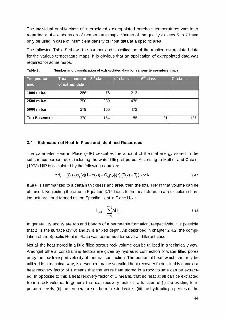
44
The individual quality class of interpolated / extrapolated borehole temperatures was later
regarded at the elaboration of temperature maps. Values of the quality classes 5 to 7 have
only be used in case of insufficient density of input data at a specific area.
The following Table 9 shows the number and classification of the applied extrapolated data
for the various temperature maps. It is obvious that an application of extrapolated data was
required for some maps.
Table 9: Number and classification of extrapolated data for various temperature maps
Temperature
map
Total amount
of extrap. data
3rd
class 4th
class 6th
class 7th
class
1000 m.b.s 286 73 213 - -
2500 m.b.s 758 280 478 - -
5000 m.b.s 579 106 473
Top Basement 370 164 58 21 127
3.4 Estimation of Heat-In-Place and Identified Resources
The parameter Heat in Place (HIP) describes the amount of thermal energy stored in the
subsurface porous rocks including the water filling of pores. According to Muffler and Cataldi
(1978) HIP is calculated by the following equation:
Az)T)z(T))(z(C))z(1)(z()z(C(H 0wwrr0 3-14
If H0 is summarized to a certain thickness and area, then the total HIP in that volume can be
obtained. Neglecting the area in Equation 3.14 leads to the heat stored in a rock column hav-
ing unit area and termed as the Specific Heat in Place Hsp,0:
2
1
zz
zz
0,sp0,sp HH 3-15
In general, z1 and z2 are top and bottom of a permeable formation, respectively, it is possible
that z1 is the surface (z1=0) and z2 is a fixed depth. As described in chapter 2.4.2, the compi-
lation of the Specific Heat in Place was performed for several different cases.
Not all the heat stored in a fluid filled porous rock volume can be utilized in a technically way.
Amongst others, constraining factors are given by hydraulic connection of water filled pores
or by the low transport velocity of thermal conduction. The portion of heat, which can truly be
utilized in a technical way, is described by the so called heat recovery factor. In this context a
heat recovery factor of 1 means that the entire heat stored in a rock volume can be extract-
ed. In opposite to this a heat recovery factor of 0 means, that no heat at all can be extracted
from a rock volume. In general the heat recovery factor is a function of (i) the existing tem-
perature levels, (ii) the temperature of the reinjected water, (iii) the hydraulic properties of the

45
investigated rock volumes and (iv) the applied geothermal utilization technique. The determi-
nation of the heat recovery factor is not trivial and is mostly executed by the help of empirical
studies (e.g. site specific numerical parameter studies).
Nevertheless, in case of a doublet system consisting of a production and injection well, both
filtered in the same reservoir, the recovery factor can be estimated in a very first approach
following an approach by Hurter and Haenel (2002):
0
inj
T)z(T
T)z(T33.0R
3-16
According to Gringarten (1978), the recovery factor for a single well use (no reinjection) is
equal to R = 0.1. The approach of Haenel and Hurter (2002) may be seen as an optimistic
assumption outlining the maximum recoverable heat in place. In praxis heat recovery factors
may vary in the range of <0.1 and 0.4.
The combination of the Specific Heat in Place and the heat recovery factor leads to the so
called “Specific Identified Resources”, which is to be seen as the upper limit of the technically
recoverable portion of heat stored in the subsurface:
0,sp1,sp HRH 3-17
In a first approach the heat recovery factor was obtained from Equation 3.16 and therefore
neglecting the hydrogeological conditions at the subsurface in order to outline the magnitude
of the maximum available heat stored in the underground for geothermal utilization. In the
later course of the study Transenergy, especially at the pilot areas, a more sophisticated ap-
proach estimating the heat recovery factor will be applied.
The calculation of both parameters for the different cases was performed on the basis of 2D
grids containing the input data.
3.5 Geo-statistical interpolation
Geo-statistical interpolation methods have been applied in order to elaborate the various
map series including:
Surface Heat Flow Densities
Temperature distribution at different depth levels
Depth distribution at different temperature levels
Distribution of specific Heat in Place and Specific Identified Resources
In the following chapters the chosen raster interpolation algorithms, which have been applied
using the software Package Surfer™, will be discussed.
3.5.1 Interpolation methods for Surface Heat Flow Density
Since different interpolation methods are available, a comparison and thus a selection of the
most satisfying interpretation had to be made. The following approaches were compared in
order to find the most suitable interpolation method:

46
Inverse Distance to a Power (IDTAP)
Kriging
Minimum Curvature
In a first step, all three methods have been applied on the data set based on the same geo-
metrical settings, which are shown in the subsequent Table 10).
Table 10: Grid line geometry for supra-regional scale data interpolation
Minimum [km] Maximum [km] Spacing [km] Number of Lines
X Direction 300 1000 1 701
Y Direction 5000 5500 1 501
Figure 22 shows the results of the applied different interpolation methods:
Figure 22: Surface Heat Flow Density map for supra-regional area from different interpolation meth-ods; a: Inverse Distance to a Power, b: Kriging, c: Minimum Curvature.
The Inverse Distance to a Power (IDTAP) method is an averaging method and uses distance
as weighting. It is fast but generates “bull’s-eye” patterns of concentric contours around indi-
vidual datum points (see Figure 22 - a). By using an iterative approach the Minimum Curva-
ture method attempts to fit a surface to all data values. It is a fast method, which generates
500000 550000 600000 650000 700000 750000 800000
Easting [m]
5100000
5150000
5200000
5250000
5300000
5350000
5400000
No
rth
ing
[m
]
[mW/m2]
35
40
45
50
55
60
65
70
75
80
85
90
95
100
105
110
115
[mW/m2]Inverse Distance to a Power Kriging
-0
10
20
30
40
50
60
70
80
90
100
110
120
130
140
150
160
170
180
Minimum Curvature[mW/m2]
a b
c

47
smooth surface, but it extrapolates values beyond the parameter range of the applied data
set (see Figure 22 - c; negative values in purple). The Kriging method is one of the most flex-
ible methods and uses trends in the map to extrapolate data (see Figure 22 – b), but it has
the same disadvantage as Minimum Curvature.
Both the fact that the values exceed the heat flow density range by applying the Minimum
Curvature method as well as the expected regional trends by using the Kriging method in-
stead of isolated bull-eye shaped anomalies, as applied by the IDTAP method, led to the
decision, that all 2D interpolation was achieved by using Kriging.
The second step was to change the statistical settings of the Kriging method (Variogram
model & search options in order to minimize artificial patterns at the SHFD map: Due to nu-
merous variogram models Kriging is a very flexible gridding method. The variogram charac-
terizes the spatial variability of a dataset. A variogram analysis consists of the experimental
variogram (black line with dots in Figure 23) estimated from the data and the variogram
model fitted to the data (blue line Figure 23). The variogram model defines the spatial
weights of the Kriging.
Figure 23: Variogram of surface heat flow density data set (default settings). Black line with dots:
experimental variogram; blue line: variogram model (linear function with nugget effect)
According to Barnes (2002), the experimental variogram is estimated by averaging one-half
the difference squared of the SFHD values over all pairs of observations with the specified
separation and direction. The variogram model can be chosen from a set of mathematical
functions, which describe spatial relationships. The appropriate model is chosen by fitting the
variogram model to the experimental model. If the experimental variogram never levels out
as in our case, the linear function is appropriate. Since the experimental model appears to
intercept with the vertical axis not at zero, a so called Nugget Effect had to be applied. The
Nugget Effect quantifies the short distance variability (i.e. spatial variations occurring at dis-
tance closer than the grid spacing). The variogram model was matched by changing the
0 20000 40000 60000 80000 100000 120000 140000
Lag Distance
0
50
100
150
200
250
300
350
400
450
500
Variogra
m
Direction: 0.0 Tolerance: 90.0Column D: HFD [mW/m2]
Nugget Effect

48
Nugget Effect and the slope of the linear function. After choosing appropriate initial values for
the Nugget Effect and the slope, a fine-tuning of the model was obtained by the option Auto-
matic Variogram Fitting. The parameters were calculated by iterative LSQ-optimization (see
Figure 24).
Figure 24: Final variogram of surface heat flow density data set (default settings); black line with dots:
experimental variogram; blue line: variogram model (linear function)
The search option is a further possibility for modifications, because it controls which data are
considered by the gridding operation when interpolating grid nodes, the maximum and mini-
mum number of data and the radius in which to look for data. By trial and error these search
parameters were determined for the surface heat flow density map (see Table 11).
Table 11: Search options for surface heat flow density map
Search radius 50 km
Number of search sectors 4
Maximum number of data in all sectors 64
Minimum number of data in all sector 2
The compiled surface heat flow density map with the above mentioned settings is shown in
Figure 25.
0 5000 10000 15000 20000 25000 30000 35000 40000 45000 50000
Lag Distance
0
50
100
150
200
250
300
350
400
Vari
ogra
m
Direction: 0.0 Tolerance: 90.0Column D: HFD [mW/m2]
Nugget Effect 143
Slope 0.004152
Anisotropy Ratio 1.305
Anisotropy Angle 82.3

49
Figure 25: Final version of the interpolated Surface Heat Flow Density map combined with the asso-ciated variogram
3.5.2 Applied Interpolation methods for Temperature and Depth Maps
(a) Temperature Maps:
The applied 2D temperature interpolation procedures to the temperature data sets were quite
similar to the one applied for the elaboration of the SHFD map. The gridding method Kriging
was used for all temperature maps based the same geometrical settings (see Table 10).
However, there was a problem with the associated variogram used for the SHFD maps
(Gaussian model) for the maps at a depth of 1000 and 2500m below surface. It was found
out by trial and error that a linear model was best fitting in order to create reasonable tem-
perature maps (Figure 26 and Figure 27).
Figure 26: Optimized temperature map at a depth of 1000m below surface applying a linear vario-gram model (optimization by auto fitting).
500000 550000 600000 650000 700000 750000 800000
Easting [m]
5100000
5150000
5200000
5250000
5300000
5350000
5400000
No
rth
ing
[m
]
25
30
35
40
45
50
55
60
65
70
75
80
85
90
95
100
105
110
115
120
125
130
[mW/m2]
0 5000 10000 15000 20000 25000 30000 35000 40000 45000 50000
Lag Distance
0
50
100
150
200
250
300
350
400
Va
rio
gra
m
Direction: 0.0 Tolerance: 90.0Column D: HFD [mW/m2]
500000 550000 600000 650000 700000 750000 800000
Easting [m]
5100000
5150000
5200000
5250000
5300000
5350000
5400000
Nort
hin
g [m
]
0 5000 10000 15000 20000 25000 30000 35000 40000 45000 50000
Lag Distance
0
10
20
30
40
50
60
70
80
Va
rio
gra
m
Direction: 0.0 Tolerance: 90.0Column D: Temperature at depth of 1000m
[°C]
15
20
25
30
35
40
45
50
55
60
65
70
75
80
85
90
95
100
Linear model

50
Table 12: Search options for temperature at 1000 m.b.s
Search radius 50km
Number of search sectors 4
Maximum number of data in all sectors 64
Minimum number of data in all sector 1
Variogram model Linear
Slope 0.000792
Anisotropy Ratio 2
Anisotropy Angle 5.18
Nugget Effect 9.4
Figure 27: Optimized temperature map at a depth of 2500m below surface (m.b.s.) applying a linear variogram model (optimization by auto fitting).
Table 13: Search options for temperature at 2500 m.b.s
Search radius 50km
Number of search sectors 4
Maximum number of data in all sectors 64
Minimum number of data in all sector 1
Variogram model Linear
[°C]
450000 500000 550000 600000 650000 700000 750000 800000 850000
Easting [m]
5050000
5100000
5150000
5200000
5250000
5300000
5350000
5400000
5450000
Nort
hin
g [m
]
3035404550556065707580859095100105110115120125130135140145150155160
Linear model
0 5000 10000 15000 20000 25000 30000 35000 40000 45000 50000
Lag Distance
0
20
40
60
80
100
120
140
160
180
200
Va
riog
ram
Direction: 0.0 Tolerance: 90.0Column D: Temperature at depth of 2500m

51
Slope 0.002817
Anisotropy Ratio 1.4
Anisotropy Angle 20
Nugget Effect 51.94
In case of the temperature map at 5000 m.b.s., the interpolation was performed without any
difficulties. The shape of the experimental model was almost linearly. Thus, a linear vario-
gram model was used for interpolation. In Figure 28 the temperature map at 5000 m.b.s. and
the associated variogram is plotted.
Figure 28: Optimized temperature map at a depth of 5000m below surface (m.b.s.) applying a linear variogram model (optimization by auto fitting).
In Table 14 the important settings for interpolation are specified.
Table 14: Search options for temperature at 5000 m.b.s
Search radius 50km
Number of search sectors 4
Maximum number of data in all sectors 64
Minimum number of data in all sector 1
Variogram model Linear
Slope 0.003163
500000 550000 600000 650000 700000 750000 800000
Easting [m]
5100000
5150000
5200000
5250000
5300000
5350000
5400000
No
rth
ing
[m
]
0 5000 10000 15000 20000 25000 30000 35000 40000 45000 50000
Lag Distance
0
50
100
150
200
250
Va
rio
gra
m
Direction: 0.0 Tolerance: 90.0Column D: Temperature at depth of 5000m
[°C]
70
80
90
100
110
120
130
140
150
160
170
180
190
200
210
220
230
240
250

52
Anisotropy Ratio 2
Anisotropy Angle 40.3
Nugget Effect 29.5
For compilation of the temperature map at the top of pretertiary basement the same gridding
method (Kriging) was applied (see Figure 29).
Since the experimental model for this temperature map didn’t level out the linear model was
used for interpolation purpose. The settings of the temperature interpolation are shown in
Table 15.
Figure 29: Optimized temperature map at the surface of the pre-Tertiary basement applying a linear variogram model (optimization by auto fitting).
Table 15: Search options for temperature at top of pre-Tertiary basement
Search radius 50km
Number of search sectors 4
Maximum number of data in all sectors 64
Minimum number of data in all sector 1
Variogram model Linear
Slope 0.003163
Anisotropy Ratio 2
Anisotropy Angle 40.3
Nugget Effect 29.5
500000 550000 600000 650000 700000 750000 800000
Easting [m]
5100000
5150000
5200000
5250000
5300000
5350000
5400000
Nort
hin
g [m
]
0 5000 10000 15000 20000 25000 30000 35000 40000 45000 50000
Lag Distance
0
200
400
600
800
1000
1200
1400
1600
1800
2000
2200
Variogra
m
Direction: 0.0 Tolerance: 90.0Column E: Temperature at top of pretert
1020
30
40
5060
70
80
90100
110
120
130140
150
160
170180
190
200
210220
230
240
250
[°C]
53
(b) Depth Maps of different temperature levels:
Depth maps of three different temperature levels, (50 °C, 100 °C and 150 °C) have been
compiled for the whole supra-regional area. Since isothermal maps were only available for
the Hungarian part, the depth information has to be interpolated from the previous generated
temperature maps.
The finite element simulation software package FEFLOWTM was used for 3D temperature
interpolation. Steady state finite element methods can be used for interpolation by applying
dirichlet or first kind (“fixed temperature”) boundary condition only and setting the material
properties homogeneous and isotropic. Through that approach the heat equation is simplified
and collapses to Laplace’s equation . The solution of this equation is independent of
any material parameter and represents a 3D interpolation based on the heat equation. This
procedure was carried out for the whole supraregional area to assure consistence.
3.5.3 Interpolation methods for Heat-In-Place and Specific Identified Resources
The calculation of Specific Heat in Place and Specific Identified Resources was basing on
the previously elaborated interpolated subsurface temperatures at depths of 1km, 2.5 and 5
km below surface (see chapter 3.5.2) as well as on interpolated petrophysical data. For the
creation of potential maps the same interpolation routines as applied for the temperature
maps (see chapter 3.5.2) have been applied.
3.6 Estimation of background heat flow densities (Lenkey L. & Raáb D.)
The following chapter treats the estimation of the background heat flow densities based on
pure conductive 3D thermal modelling. Although the background HFD will not be displayed in
terms of individual maps, the achieved results will help later to outline and classify existing
thermal convection zones caused by circulating thermal water. Therefore the following chap-
ter gives a detailed overview about the applied methodologies and workflows.
This chapter was compiled by Lenkey, L. and Raáb, D. on behalf of the Geological Institute
of Hungary.
3.6.1 Introduction
We calculated the three-dimensional temperature distribution in the lithosphere under the
area of the TE project assuming conductive heat transport using the finite element modelling
software Comsol Multiphysics. We made a steady-state model and two transient models; one
of them takes into account the stretching of the lithosphere during Middle Miocene, and the
other additionally takes into account the thermal effect of the Neogene and Quaternary sedi-
mentation.
We compared the modelled surface heat flow density and temperatures in 1 and 2.5 km
depths with surface heat flow density map (Figure 25) and temperature maps (Figure 26and
Figure 27) based on observations. We also compared the modelled temperatures with tem-
peratures measured in wells. We assume that the best fit model describes the conductive
temperature field in the lithosphere in the study area. In the best model we calculated the

54
heat flow density at the Mohorovicic discontinuity. It can be used as thermal boundary condi-
tion prescribed at the bottom in the thermal models of the pilot areas, in which groundwater
flow and coupled heat transport will be modelled.
3.6.2 Description of the chosen modelling approach
(a) Physical settings
Assuming conduction the distribution of temperature in solid materials is governed by the
following equation (e.g. Carslaw and Jaeger, 1959):
A)z
T(
z)
y
T(
y)
x
T(
xt
Tc
3-18
Where T is temperature, c is specific heat, is density, t is time, λ is thermal conduction, and
A is volumetric heat production rate. c, , λ and A can vary in space. If the temperature does
not change with time the thermal field is called to be in a steady-state condition. In that case
the left side of the equation is equal to zero.
We solved equation 3.18 applying the finite element method using Comsol Multiphysics™ in
three dimensions. The average length of an edge of a tetrahedral element in the model was
2 km.
(b) Geometrical settings
The model was built in UTM33 coordinate system and it includes three layers with individual
material properties (Figure 30). These layers constitute:
(i) sedimentary rocks,
(ii) crust,
(iii) lithospheric mantle
They are bordered and divided by the following horizons: (a) surface, (b) the depth of the
pre-Tertiary basement, (c) the Mohorovicic discontinuity, and (d) the bottom of the litho-
sphere (see Figure 31). In case of the steady-state model the bottom of the lithosphere cor-
responds to the observed lithosphere shown in Figure 31d. In case of the transient models
the bottom horizon of the lithosphere was set at a depth of 125km, except in those areas
where the observed thickness is larger than 125km. In those areas the observed lithospheric
thickness (see Figure 31d) was used. The reason therefore is the stretching model of the
lithosphere (McKenzie, 1978), which was used to obtain the initial temperature distribution in
the lithosphere of the transient models. These three layers were filled up with material prop-
erties.

55
Figure 30: Geometrical model applied for the estimation of the background heat flow density.
Figure 31: The horizons which bound and separate the layers comprising the model. a) Surface to-
pography, b) Depth to the pre-Tertiary basement, c) Depth to the bottom of the crust (Lenkey, 1999), d) Depth to the bottom of the lithosphere (Lenkey, 1999).

56
(c) Thermal parameters of rocks
Considering equation 3.18 the most important material parameters are the thermal conduc-
tivity and heat production of rocks. Specific heat and density only play a role in transient
models. We assumed that except for the sediments the crust is homogeneous. We made this
assumption, because we do not know in detail the spatial extent of the different types of
rocks in the crust, e.g. the thickness of Triassic carbonates in the Transdanubian Central
Range (TCR) is known only in a few wells. On the other hand the difference between the
thermal conductivities of crystalline, metamorphic rocks and limestones is less than the con-
trast in thermal conductivities of the sediments and their basement. Thus, in spite of the sim-
plification of a homogeneous crust, the model takes into account the first order features in
the thermal conductivities. Most of the temperature measurements and thus heat flow density
estimates were carried out in the sedimentary basins. Therefore, the model results can be
fitted in these areas and the model remains less constrained in the areas of the outcrop of
the pre-Tertiary basement.
Thermal conductivity of crust and mantle were taken from Kappelmeyer and Haenel (1974)
and Zoth and Haenel (1988) (see also Table 7). The thermal conductivity of sediments varies
both horizontally and vertically, due to variations in their composition (e.g. shales, marls,
sand, and sandstones) and compaction. In the model we used the same thermal conductivi-
ties of sediments, which were applied in the heat flow density estimates in the Transenergy
project. In the Vienna and Styrian basins we assigned the values given in Table 7. As the
material parameters are given for different age horizons, we had to further subdivide the Ne-
ogene sediments. We estimated the thickness of the sediments with different ages using
stratigraphic sections by Kovač et al. (2004) for the Vienna Basin and by Goldbrunner (2000)
for the Styrian basin. In the rest of the study area we chose wells, in which we knew, or we
calculated the thermal conductivity of sediments.
In Hungary the thermal conductivity of sediments was taken from the Geothermal Database
of Hungary (Dövényi, 1994).
In the Slovakian wells we calculated the thermal conductivity in the following way. In the “At-
las of the geothermal energy of Slovakia” (Franko et al., 1995) temperatures in wells are pre-
sented for 500m intervals, and the heat flow density is also given for the same wells. We cal-
culated the temperature gradients for 500m intervals. By assuming a constant heat flow den-
sity we determined the thermal conductivities from the Fourier equation.
Finally, we chose those Slovenian wells, in which thermal conductivity of sediments were
published (Ravnik, 1991, Ravnik et al., 1995).
In the 3D model the thermal conductivity of each element must be prescribed. The thermal
conductivity of the sediments in a given place was calculated by horizontal and vertical ex-
trapolation using the values in the wells or the values given in 3D grids in the Vienna and
Styrian basins. The extrapolation was done by the modelling software Comsol Multiphys-
ics™.

57
The volumetric heat production rate in the crust and sediments was set to 1W/m3. This val-
ue in the sediments is supported by measurements (Table 7). However, in the crust the radi-
ogenic heat production rate is somehow arbitrary. Granites show higher (2-3W/m3, Rybach
and Cermak, 1982) and lower crustal granulites lower (0.2-0.5W/m3, Rybach and Bunte-
barth, 1984) heat production rates. In general, it was assumed that heat production decreas-
es with depth. Due to limited information about the crustal structure in the study area we
chose an average crustal heat production rate. We checked our choice of thermal parame-
ters by calculating the steady-state geotherms in the continental lithosphere by applying
equation 3.18.
In case of an average continental crustal thickness of 35km, and a lithospheric thickness of
125km with an assumed temperature of 1300°C at its bottom, and 10°C at the surface of the
model, 1W/m3 heat production rate together with the crustal and mantle thermal conductivi-
ties (Table 7) result in surface heat flow density of 63mW/m2, which is close to the average
continental value of 57mW/m2 (Sclater et al., 1980). Therefore, we accepted the heat produc-
tion rate in the crust and the thermal conductivities of the crust and mantle. The steady-state
geotherm calculated with the above conditions and parameters are presented in Figure 32.
The rock density of crust and mantle material corresponds to the average values (Parsons
and Sclater, 1977). We calculated the specific heat of rocks from the definition of the thermal
diffusivity (): = λ/c. Thermal diffusivity was kept constant in the whole lithosphere (8.23 x
10-7 m2/s, after Royden and Keen, 1980), so the specific heat was determined from the given
density and thermal conductivity of rocks.
Figure 32: Geotherms in the lithosphere. Black line: steady state temperature, which exists in a 125 km
thick lithosphere, with35 km thick crust. Values of the thermal parameters are shown in Table 8.

58
Red line: initial geotherm (t=0 time) calculated from the steady state geotherm by stretching the lithosphere (Trans-T model). Blue line: initial geotherm (t=0 time) calculated from the initial geo-therm of the Trans-T model by placing 7 km thick sedimentary pile with temperature of 10 °C on the top of the crust (Trans-Sed model).
(d) Initial and boundary conditions
For simplicity reasons the surface temperature was kept constant at 10°C. In case of steady-
state model the temperature at the bottom of the lithosphere was also constant 1300°C. In
case of transient models the above conditions were applied at locations, where the depth of
the bottom of the lithosphere is larger than 125km. Where the lithosphere is thinner than
125km, there 1300°C was prescribed at 125km depth (see geometry of the model, chapter
3.6.2 b). The vertical boundary planes of the model were insulating.
In case of transient heat transport processes the solution of equation 3.18 also depends on
the initial temperature distribution. The most important geological processes resulting in tran-
sient thermal field are a) the change of the surface temperature due to palaeo-climatic tem-
perature variations, b) volcanism, c) tectonic events, d) sedimentation and erosion.
a) The Pannonian Basin palaeo-climatic effects mainly influence the subsurface tem-
perature at depths above 500m below surface (Demetrescu et al., 2001). In most
cases we compared temperatures measured deeper than 1km with the calculated
model temperatures, therefore we neglected the palaeo-climatic effects.
b) The effusive material from volcanic activity does not have effect on the subsurface
temperature. It is mostly the magma chamber, which warms up the host rock. Several
model calculations showed that a normal size magma chamber cooled down in less
than 1 Ma year in the absence of additional magma supply (Raáb, 2011). As volcanic
activity in the Styrian basin and the Little Hungarian Plain decayed more than 1 Ma
(Pécskay et al., 1995). Therefore we did not take volcanism into account for the tran-
sient conductive models.
c) The strongest effect on the subsurface temperature derives from tectonic events. The
Pannonian basin was formed during the Early-Middle Miocene by lithospheric stretch-
ing as it is evidenced by the thin lithosphere and crust, normal faults bounding the
sediment filled depressions, and high heat flow density (Royden et al., 1983a, Roy-
den and Horváth, 1988). It was shown by numerous studies that the observed sub-
sidence rate of the basement and the heat flow density in the Pannonian basin can
be reproduced applying Royden and Keen’s (1980) non-uniform lithospheric stretch-
ing model (Royden et al., 1983b, Royden and Dövényi, 1988, Lankreijer et al., 1995,
Sachsenhofer et al., 1997, Lenkey, 1999).
According to the stretching model instantaneous stretching of the lithosphere leads to
high initial geothermal gradient, and thus high initial heat flow density (Figure 32). Fol-
lowing stretching the high temperature in the lithosphere slowly decreases and the
original HFD is approached after a time period of about 100 Ma (McKenzie, 1978).
We modelled the transient thermal effect of stretching using the crustal and mantle
stretching factors derived by Lenkey (1999). We compressed the steady-state geo-

59
therm in the lithosphere according to the stretching factors, and thus we received the
initial temperature-depth function (Figure 32). We repeated the above process in a
grid with 5km spacing. In those places, where stretching did not occur we kept the
steady-state geotherm calculated with the geometries given in Figure 31.
We assumed that the stretching of the lithosphere was instantaneous, and it have oc-
curred 17.5 Ma ago. This moment was the starting time of the transient calculations.
The stretching factors were calibrated to reproduce the present day basement depth
and sedimentation corrected heat flow density smoothed by a low pass filter with 100
km cut-off wavelength (Lenkey, 1999). We wanted to obtain the same cooling rate of
the initial thermal anomaly in the lithosphere in our model than in the stretching mod-
el, therefore we applied the same thermal diffusivity (κ=8.23*10-7m2/s, see in the
above section) as Lenkey (1999) after Royden and Keen (1980).
The stretching model and the obtained results are referd in the following as Trans-T.
d) Sedimentation reduces the subsurface temperature as the newly deposited sedi-
ments have “cold” surface temperature and it therefore takes time until the sediments
are heated up (e.g. Lucazeau and Le Douaran, 1985). Erosion has the opposite effect
on the temperature. In the model area sediments were accumulated over several kil-
ometres thickness in the basin areas during the Neogene and Quaternary, and ero-
sion in the peripheral areas has been active since Late Miocene-Pliocene times. Ac-
cording to Lenkey (1999) mainly sedimentation affected the temperature field and the
heat flow density regime. We applied a simple model in calculating the thermal effect
of sedimentation. We assumed that all sediments had been deposited before the start
of the calculation, and they had initial temperature of 10°C (Figure 32). Below the
sediments the temperature-depth function was obtained by shifting downward the ini-
tial geotherm of the stretched lithosphere with the thickness of sediments.
The model which takes into account the sedimentation and the stretching is referres
in the following as Trans-Sed.
4 Results
4.1 Surface Heat Flow Density Map
The Surface Heat flow Density (SHFD) represents the overall heat flow density including
conductive as well as advective heat transport at the uppermost part of the subsurface. It
was calculated from observed borehole temperatures for individual wells. The SHFD is di-
rectly correlating with the geothermal conditions. That means an elevated SHFD is accom-
panied by a high geothermal gradient. Therefore the elaborated map, which can also be
found at Enclosure 1, allows differing between regions with favourable and less favourable
geothermal conditions. However, it does not directly outline or estimate existing hydrogeo-
thermal reservoirs or plays. For that reason a SHFD can be seen as the first step towards the

60
evaluation of the geothermal resources in a specific region. Nevertheless, the following op-
tions for further calculations and interpretation can be gained from the elaborated map:
Geothermal boundary conditions for local to regional scale geothermal models at
the pilot areas.
Evaluation of the entire amount of heat flowing into the project area for thermal bal-
ancing.
Identification of areas affected by the circulation of subsurface waters.
The elaborated map is based on around 1200 input data in the range of <5 to >185mW/m²
(see also Figure 33). The average calculated SHFD at the Transenergy project area is repre-
sented by 77.69±21.50mW/m², which is above the continental average. The distribution of
calculated SHFD values shows a clear maximum at the class of 65 to 70mW/m², which is
accompanied by an asymmetric slope with a slighter decrease towards values of enhanced
SHFD.
A 3 – colour scheme was applied to the SHFD map showing a colour range from dark blue
(low values) to white (average) and dark red (high) values in order to easily outline areas of
favourable and less favourable geothermal conditions (Figure 34). The pattern of the interpo-
lated SHFD map show clear enhanced conditions at the south-western part of the project
area covering parts of the Styrian- and Mura – Zala Basin. In opposite to this lowered geo-
thermal conditions can be found at the margin of Eastern Alps (north-western part of the pro-
ject area) and the Transdanubian Range (eastern part of the project area). At both regions
crustal thickening in combination with massive inflow of cold meteoric water can be seen as
major reason for the lowered geothermal conditions.
Figure 33: Statistical overview on the applied input data in order to elaborate the SHFD map.

61
Figure 34: Surface Heat Flow Density map of the entire project area
Several local to regional scale geothermal anomalies are superimposed to the regional –
supra-regional scale pattern of the SHFD values. Most of these low scale anomalies are
caused by the circulation of subsurface water. Despite of the influence of circulating subsur-
face waters, a regional scale attenuation of the geothermal conditions in the central and
northern parts of the Vienna Basin (north-western part of the project area) is assumed to be
linked to non-steady-state conditions due to fast sedimentation in the Vienna Basin in combi-
nation with enhanced crustal thickness.
4.2 Temperature Map series
The temperature map series shows the distribution of subsurface temperatures at depth lev-
els of 1000, 2500 and 5000m below surface in order to give an overview on the expectable
rock temperatures in certain regions. They have been compiled from individually interpolated
and extrapolated borehole temperatures. A statistical overview of the interpolated input data
can be found in Figure 35, while the maps themselves are shown in Figure 36 and Figure 37.
Furthermore the expected temperature at the top of the pre-Tertiary basement have been
interpolated from the temperature map series in order to give an overview about the expect-
able maximum subsurface temperatures at the Tertiary basin fillings, which constitute a rele-
vant hydrogeothermal reservoir at many regions within the project area (e.g. western Panno-
nian Basin).
The entire temperature map series can also be found in Enclosures 2a – 2d.

62
At a depth of 1000m below surface (m.b.s) the observed average rock temperature corre-
sponds to 49.4±9.4°C. Significant positive temperature anomalies are linked to local to re-
gional scale ascent and discharge areas of hot subsurface waters, as for example to be ob-
served in a significant anomaly at Héviz westwards of lake Balaton. In opposite to this cool
areas predominately correspond to the descent and infiltration paths of cold meteoric waters.
Such patterns indicate the estimated boundaries of confined hydrodynamic flow systems
including recharge and discharge areas. It can be summarized, that the patterns of the sub-
surface temperatures at depths up to 1000 meters below surface are more likely to corre-
spond to surface near hydrodynamic systems than to large scale crustal structures.
The distribution of temperature at a depth of 2500 m.b.s shows an average value of
100.8±13.1°C. The comparison with the mean value at a depth of 1000 m.b.s. results in an
average geothermal gradient for the project area of 3.4°C/100m, which is again slightly
above the global average. The pattern of the subsurface temperatures at this depth are al-
ready influenced by large scale crustal structures, as enhanced conditions with temperature
levels of above 130°C can be observed at parts of the Styrian and Mura – Zala Basin (see
also chapter 4.1).

63
Figure 35: Statistical overview on the input data applied on the elaboration of the map series show-ing the temperature distribution at a depth of 1000, 2500 and 5000m below surface

64
Figure 36: Distribution of subsurface temperatures at depth levels of 1000m and 2500m below sur-face.

65
Figure 37: Distribution of temperature at a depth of 5000m below surface and at the top of the pre-Tertiary basement.
At a depth level of 5000m below surface the mean interpolated or extrapolated formation
temperature is corresponding to 178.9±18.5°C, which in turn leads to an average geothermal

66
gradient of 3.12°C/100m between the depth intervals of 2500 and 5000m. Except for the
margin of the Eastern Alps in the western and northwestern part of the project area, the
interpolated temperature maps now strongly correlates with large scale crustal structures. At
the margin of the Eastern Alps there are deeply infiltrating fresh water circulation systems
known, which still lead to an attenuation of the subsurface temperature regime. However, it
has to be kept in mind, that at the depth level of 5000m below surface most apllied data are
gained from extrapolation and therefore probably afflicted with a significant range of
uncertainity.
The temperature map of the pre-Tertiary surface (see Figure 37) was compiled from
individually prepared borehole related input data. The map itself is combined with
outcropping areas of the pre-Tertiary basement rocks and depth contours of the basement
within the basins in order to enable an easy interpretation of the map. Once again a 3 – color
scheme was applied, where dark blue to white colors reflect subsurface temperatures below
100°C and white to dark red colors in turn outline areas above 100°C. The 100°C isotherm
was chosen with repsect to the generation of electric power by applying geothermal
methods. The resulting patterns of course strongly reflect the depth of the pre-Tertiary
basement. Regions with expected maximum temperatures at the basin filling above 100°C
are only to be expected at (i) the central and northern part of the Vienna Basin, (ii) the
eastern Styrian Basin, (iii) parts of the Mura – Zala Basin and (iv) the Danube Basin. The
latter region is supposed to serve the highest temperatures within the basin fillings in the
project area with expected maximum temperatures of more than 220°C eastwards of the city
of Györ.
4.3 Contour map series of specific isotherms
Based on the previously elaborated temperature maps, depth contour of the (i) 50°C, (ii)
100°C and (iii) 150°C isotherm have been calculated by using FEFLOW™. This map series
intend to give an overview about the minimum depths of reservoir in order to guarantee a
certain reservoir temperature for energetic geothermal utilization. The isotherm of 50°C (i)
was assumed to be a critical value for low temperature applications (e.g. balneological use
combined with green house or facility heating). The 100°C isotherm (ii) is seen as a critical
value for electric power generation based on binary circle technology (e.g. ORC process), as
well as the 150°C isotherm (iii), which constitutes the boundary to direct electric power gen-
eration based on steam turbines. All maps are shown in the subsequent Figure 38 to Figure
40 and can also be found in Enclosure 3a to 3c.
The depth of the 50°C isotherm (Figure 38) between 600 meters at discharge areas of hot
thermal waters (e.g. Heviz, Oberlaa – Vienna) and 2700 meters at the infiltration zones of
fresh surface waters (Eastern Alps, Bakony Mountains). It has to be pointed out, that this
variation of depths coincides with range of investments for drilling of more than €1.5 Mio. In
general the depth of the 50°C isotherm is situated around 1000 to 1200m.

67
Figure 38: Depth contour map of the 50°C isotherm.
Figure 39: Depth contour map of the 100°C isotherm.

68
The depth of the 100°C isotherm varies between the range of 1500m below surface (Lake
Heviz and other parts of the Zala Basin) and 5100m (deep infiltration zones at Eastern Alps
and Bakony Mountains). The mean utilization depths are expected at around 2250 to 2500m
below surface. The pattern of the calculated depth contours is still quite similar to the ones of
the 50°C isotherm. They clearly point out deep circulating infiltration zones of hydrodynamic
systems.
In opposite to this, the pattern of the 150°C isotherm is more corresponding to crustal struc-
tures, showing favourable utilization depths at southwest – northeast heading zone covering
the eastern Styrian-, the entire Mura Zala Basin as well as the central and north-eastern
parts of the Danube Basin. Referring to the interpolated contours minimum reservoir depths
in order to reach rock temperatures of 150°C exist around 2700 to 2800m, while the average
depths are to be expected around 4000 to 4200m below surface.
Figure 40: Depth contour map of the 150°C isotherm.
4.4 Geothermal Potential Map series
The geothermal potential map series contains the parameter “Specific Heat in Place” and
“Specific Identified Resources”. Although the latter parameter contains the term “resources”,
both parameters have to be understood as theoretical potentials limiting the theoretically
available heat content in the subsurface for geothermal utilization, as they are more or less
neglecting existing geothermal plays. Nevertheless, they are able to provide crucial infor-
mation about favourable and non-favourable regions with respect to the geothermal regime
of the subsurface.
The following maps were generated:

69
Specific Heat in Place for Neogene sediments
Specific Heat in Place for 50m upper part of the pre-Tertiary basement
Specific Heat in Place from surface until 5000 m.b.s
Specific Heat in Place from surface until 7000 m.b.s
Specific Identified Resources for Neogene sediments
Specific Identified Resources for 50m upper part of the pre-Tertiary basement
Specific Identified Resources from surface until 5000 m.b.s
Specific Identified Resources from surface until 7000 m.b.s
All elaborated maps are presented in the subsequent figures from Figure 41 to Figure 43 and
can also be found at Enclosure 4a to 4h.
The Specific Heat in Place at the sedimentary basin fillings is strongly corresponding to are-
as of great depths of the basement, which are in turn offering high subsurface temperatures.
The highest values at a level of up to 2400GJ/m² can be found at the central part of the Dan-
ube Basin westwards of the city of Györ, as in this region the sedimentary basin fillings reach
maximum thicknesses of more than 7000 meters. Another hot spot can be found at the trans-
boundary region between Hungary and Slovenia within the Mura – Zala Basin. At other rele-
vant basin regions, such as the central Vienna Basin or the Styrian Basin the calculated
Specific Heat in Place reaches only half of the level of the previous mentioned regions.
The Specific Heat in Place at the uppermost 50m of the pre-Tertiary basement can be un-
derstood as the theoretical potential of petrothermal utilization as potential hydrogeothermal
plays are neglected in this assessment. In this context stored subsurface heat may be ex-
tracted by fracturing and artificial circulation of fresh surface water using geothermal doublet
or multiple techniques. Due to the reduced thickness of the investigated rock column (50 me-
ters versus up to several kilometers at the sedimentary basin fillings) the calculated Specific
Heat in Place reaches levels of only 2% of the heat stored in the sedimentary basin fillings.
Nevertheless, the pattern of the calculated Specific Heat in Place strongly follows the pattern
observed at the sedimentary fillings, showing strong positive anomalies near the city of Györ
and the trans-boundary region of Hungary and Slovenia. .
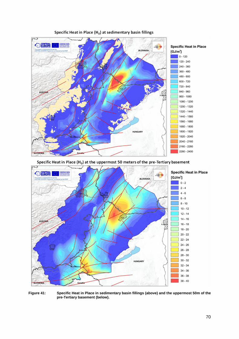
70
Figure 41: Specific Heat in Place in sedimentary basin fillings (above) and the uppermost 50m of the pre-Tertiary basement (below).

71
Figure 42: Specific Heat in Place in uppermost 5km (above) and the uppermost 7km of the Earth’s Crust (below).

72
Both results, the Specific Heat in Place of the uppermost 5km and 7km of the Earth’s Crust
show similar patterns, which are strongly governed by the temperature regime of the subsur-
face and to a minor extend to the geological build-up of the investigated rock column. The
calculated Specific Heat in Place values vary between the range of 400GJ/m² to 1600GJ/m²
for the uppermost 5km of the subsurface and between 800GJ/m² and 3000GJ/m² at the up-
permost 7km of the Earth’s Crust. Both maps imply enhanced heat content along a south-
west to northeast heading central zone of the project area.
Figure 43: Specific Identified Resource map series
The pattern of the various maps showing the Specific Identified Resources are identical to
the maps showing the Specific Heat in Place, as this parameter is directly derived from the
Specific Heat in Place by applying a heat recovery factor, which is proportional to the tem-
perature, and show that approximately 33% of the entire stored heat can be utilized.
4.5 Distribution of Background Heat Flow Density (Lenkey L. & Raáb D.)
We present the results in the forms of temperature-depth curves along control wells, temperature maps in 1km and 2.5km depths and heat flow density maps. The model is best constrained along those wells, where the thermal conductivity of sediments is known. We chose a few wells out of them, in which temperature measurements were made. The modelled and ob-

73
served temperatures along these control wells are shown in the subsequent
Figure 44 and Figure 45.

74
Figure 44: Observed and modelled temperatures in control wells in the northern part of the area.
Black squares: observed temperatures, black line: steady-state temperature, red line: tempera-ture in the Trans-T model calculated from the initial geotherm after 17.5 Ma, blue line: tempera-ture in the Trans-Sed model calculated from the initial geotherm after 17.5 Ma. Thermal pa-rameters are given in Table 7, the boundary conditions are described in the text.

75
Figure 45: Observed and calculated temperatures in control wells in the southern part of the area.
For detailed explanations see Figure 44
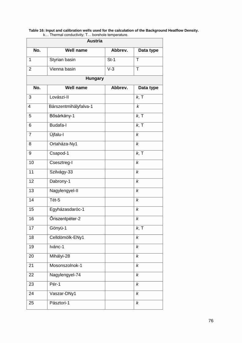
76
Table 16: Input and calibration wells used for the calculation of the Background Heatflow Density.
k… Thermal conductivity; T… borehole temperature.
Austria
No. Well name Abbrev. Data type
1 Styrian basin St-1 T
2 Vienna basin V-3 T
Hungary
No. Well name Abbrev. Data type
3 Lovászi-II k, T
4 Bárszentmihályfalva-1 k
5 Bősárkány-1 k, T
6 Budafa-I k, T
7 Újfalu-I k
8 Ortaháza-Ny1 k
9 Csapod-1 k, T
10 Csesztreg-I k
11 Szilvágy-33 k
12 Dabrony-1 k
13 Nagylengyel-II k
14 Tét-5 k
15 Egyházasdaróc-1 k
16 Őriszentpéter-2 k
17 Gönyü-1 k, T
18 Celldömölk-ENy1 k
19 Ivánc-1 k
20 Mihályi-28 k
21 Mosonszolnok-1 k
22 Nagylengyel-74 k
23 Pér-1 k
24 Vaszar-DNy1 k
25 Pásztori-1 k

77
26 Bak-5 k
27 Szombathely-II k
Slovakia
No. Well name Abbrev. Data type
28 Galanta FGG-1 k, T
29 Galanta FGG-2 k
30 Galanta FGG-3 k
31 Cilistoc FGC-1 k
32 Dunajska Streda DS-1 k
33 Dunajska Streda DS-2 k
34 Králova pri Senci VMK-1 k
35 Calovo C-1 k
36 Chorvátsko Grob FGB-1 k
37 Rusovce HGB-1 k
38 Láb L-90 k
39 Rohoznik R-1 k, T
40 Závod ZA-57 k
41 Ciliska Radvan CR-1 k
42 Horná Poton FGHP-1 k
43 Topolovec VTP-11 k, T
Slovenia
No. Well name Abbrev. Data type
44 BH-2 T
45 BH-424 T
46 Ljutj-1 k, T
47 Petisovci-7/88 Pg-7/88 k
48 Petisovci-1/91 Pec-1/91 k
49 Murski Gozd-6 Mg-6 k, T
50 Maribori-1/90 Mb-1690 k

78
The stretching model (Trans-T) predicts the highest and the combined stretching-
sedimentation model (Trans-Sed) predicts the lowest temperatures. The steady-state model
is either equal to the Trans-Sed model (mainly in the northern part of the area), or is between
the two transient models (some wells in the southern part). In the northern part of the Vienna
basin and Danube basin the steady-state model and the Trans-Sed model fit to the observa-
tions, and the Trans-T model overestimates the temperature. In the central and southern part
of the Danube basin-Little Hungarian Plain the Trans-T model is the best, the steady-state
model and the Trans-Sed model underestimate the temperature. In the Bősárkány-1 well the
deeper temperatures are higher than they would be in case of extrapolating the temperature
from shallower depths. As the deeper temperatures are more reliable, thus either the shal-
lower values are false, or groundwater flow is occurring in the porous sediments in the upper
part of the well. At the location of Gönyü-1 well groundwater flow takes part in the carbonatic
basement. That explains why all models predict higher temperatures than the observed
ones. In the Styrian basin and in SW Hungary the Trans-T model fits to the observations. In
Slovenia, except the Ljutj-1 well, the models underestimate the temperature, but still the
Trans-T model is closest to the observations. In the Ljutj-1 well the Trans-Sed and the
steady-state models fit to the observed temperatures. However, the temperature gradient in
the Ljutj-1 well seems to increase with depth, therefore we suspect, that there is downward
groundwater flow near the well.
The Trans-Sed model is either equal to the steady-state model or it misfits to the observa-
tion, therefore we rejected this model. In the following we present temperature maps and
heat flow density maps for the steady-state and Trans-T models.
The elaborated steady-state pure conductive 3D model was compared to the temperature
maps at depths of 1000m below surface and 2500m below surface as well as to the surface
heat flow density maps (see Figure 46 to Figure 48).
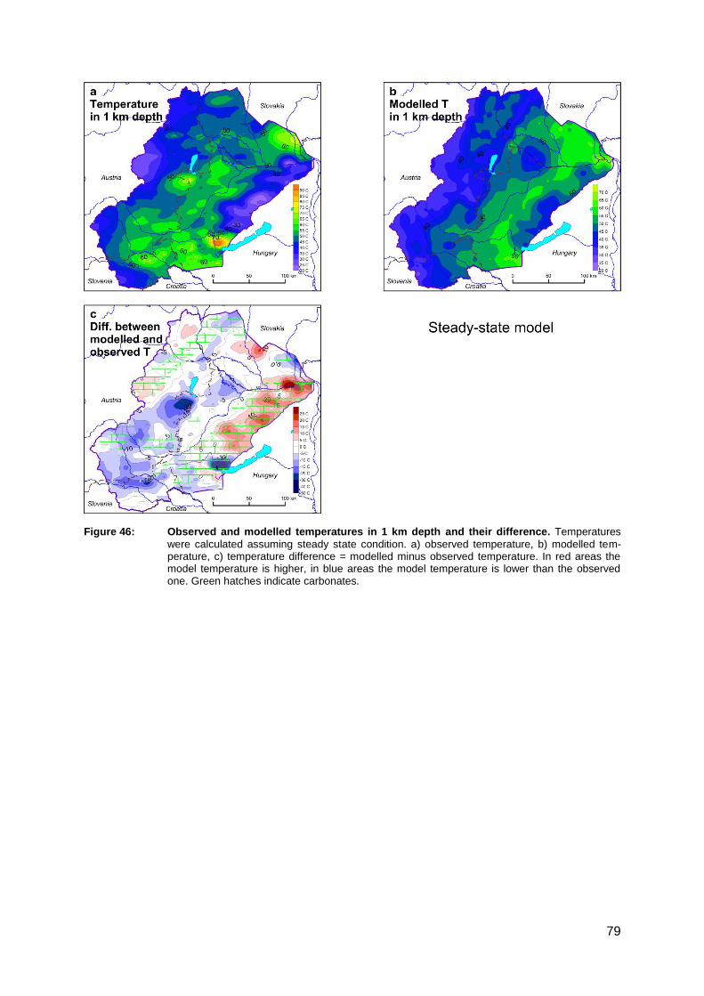
79
Figure 46: Observed and modelled temperatures in 1 km depth and their difference. Temperatures
were calculated assuming steady state condition. a) observed temperature, b) modelled tem-perature, c) temperature difference = modelled minus observed temperature. In red areas the model temperature is higher, in blue areas the model temperature is lower than the observed one. Green hatches indicate carbonates.

80
Figure 47: Observed and modelled temperatures in 2.5 km depth and their difference. Temperatures
were calculated assuming steady state condition and using geometry given in Fig. 2. a) ob-served temperature, b) modelled temperature, c) temperature difference = modelled minus ob-served temperature. In red areas the model temperature is higher, in blue areas the model tem-perature is lower than the observed one. Green hatches indicate carbonates.

81
Figure 48: Observed and modelled heat flow densities and their difference. Heat flow density was
calculated assuming steady state condition. a) observed heat flow density, b) modelled heat flow density, c) difference in heat flow density = modelled minus observed values. In red areas the model HFD is higher, in blue areas the model HFD is lower than the observed one. Green hatches indicate carbonates. Black dots indicate the location of control wells.
We can interpret the modelled heat flow density (Figure 48 - b) easiest. As the thickness of
the lithosphere decreases from NW towards SE (Figure 31d), and the temperature at the
base of the lithosphere is fixed, the geothermal gradient in the lithosphere, and thus the heat
flow density increases towards SE. This trend is slightly perturbed by the variation of the
crustal thickness and thermal conductivity. In those places where the crust is thinner, less
heat is produced. Sediments have lower thermal conductivity than the crust, thus heat flow
density is slightly diverted towards the basement flanks. When these two effects are super-
posed, like in the Little Hungarian Plain-Danube basin, the heat flow density is a little bit re-
duced relative to the surrounding areas. This reduced heat flow density is the reason of the
low predicted temperature in the centre of Little Hungarian Plain relative to the surroundings
(see Figure 46 and Figure 47). There is an apparent contradiction between the modelled
temperature and heat flow density in the SE part of the study area. The heat flow density is
constant or slightly increases towards SE, but the temperature decreases. This is due to the
fact, that towards SE the thickness of sediments reduces, therefore the average thermal

82
conductivity increases, which in turn leads to a reduction of the geothermal gradient accord-
ing to the Fourier Law of thermal conduction.
The difference between the modelled and observed quantities is presented in part -c- of Fig-
ure 46 to Figure 48. Positive values align with modelled data higher than the observed one,
negative values have the opposite meaning.
In the Transdanubian Central Range and the SE part of the Little Hungarian Plain the mod-
elled heat flow density and temperatures are higher than the observed ones. In these areas
there is intensive downward karstic water flow in the carbonatic rocks comprising the base-
ment, which results in lower temperatures. There is similar situation in the Vienna basin, but
there the thermal anomaly is smaller. In other areas the steady-state model in general pre-
dicts lower temperatures and heat flow density than it is observed (blue patches in part -c- of
Figure 46 to Figure 48).
There are two really locally confined, but significant temperature anomalies, where the ob-
served temperature is higher than the modelled one: In the SW corner of the Lake Balaton
and S to the Fertő-tó/Neusiedlersee. These are discharge areas with upwelling warm
groundwater. In other places, like in the SW part of the study area and in the Little Hungarian
Plain the predicted low temperatures and heat flow density are difficult to explain. These are
either discharge areas too, or the heat flow density from the mantle is higher. We think that
the second choice is more likely.
The heat flow density in the steady-state model strongly depends on the lithospheric thick-
ness. However, lithospheric thickness data are not available from the Styrian basin and the
Zala-Mura-Drava basins, where the misfit is largest between the observations and the model
results. The lithospheric thickness in this area is based on interpolation from distant data.
Additionally, we know that the steady-state condition in the area is not fulfilled. This was the
reason to apply the stretching model. As the stretching factors are based on the heat flow
density we expected a better fitting to the observed data. The results of the Trans-T model
are shown in Figure 49 to Figure 51.
In case of the temperatures and heat flow density the fit between the observed and modelled
data improved significantly. In the SW area the observed heat flow and temperatures are still
higher than the predicted ones, but the difference is reduced to range, which can be ex-
plained either by convection or local conduction phenomena. We note that in the SW area
the modelled heat flow density misfits to the observations, but the model temperatures fit to
the observations. One way to resolve this contradiction is if we assume that maybe we used
lower thermal conductivities in the modelling than those ones, which were used in the heat
flow density estimates. On the other hand, there are indications that upward groundwater
flow occurs along faults in the area (Kraljic et al., 2005).
The thermal anomalies of the karstic areas (TCR, Vienna basin) are present in this model
too. In the central area the model fits to the observations. There is a new misfit in this model
compared to the steady-state model: the transient model predicts higher temperatures in the
NE part of the Danube basin. However, this misfit may also indicate that downward ground-
water flow occurs in the porous sediments, which outcrop at the feet of the Western Carpa-

83
thians. At this stage it is not possible to decide if this is an “overshooting” of the model or
groundwater flow can explain the thermal field.
Figure 49: Observed and modelled temperatures at a depth of 1 km and their difference. Tempera-
tures were calculated from the Trans-T model. a) observed temperature, b) modelled tempera-ture, c) temperature difference = modelled minus observed temperature. In red areas the model temperature is higher, in blue areas the model temperature is lower than the observed one. Green hatches indicate carbonates.

84
Figure 50: Observed and modelled temperatures in 2.5 km depth and their difference. Temperatures
were calculated from the Trans-T model. a) observed temperature, b) modelled temperature, c) temperature difference = modelled minus observed temperature. In red areas the model tem-perature is higher, in blue areas the model temperature is lower than the observed one. Green hatches indicate carbonates.

85
Figure 51: Observed and modelled heat flow densities and their difference. Heat flow density was
calculated from the Trans-T model. a) observed heat flow density, b) modelled heat flow densi-ty, c) difference in heat flow density = modelled minus observed values. In red areas the model HFD is higher, in blue areas the model HFD is lower than the observed one. Green hatches in-dicate carbonates. Black dots indicate the location of control wells.
5 Summary and Conclusions
In the following chapter all main results will be summarized and interpreted with respect to
the aims of the project Transenergy.
5.1 Surface Heat Flow Density and temperature maps
The surface heat flow density (Enclosure 1) and temperature maps (Enclosure 2a-2d) indi-
cate that in some parts of the supra-regional area positive geothermal anomalies occur in the
subsurface. Therefore the elaborated maps represent a first step towards the evaluation of
the geothermal resources in specific regions.
The south-western part of the project area covering the parts of the Styrian and Mura – Zala
Basin is a region with favourable geothermal conditions (> 120mW/m2). The increased HFD
values (in the Mura – Zala Basin) are related to the convection zones in the pre-Tertiary

86
basement rocks and to various geological conditions like e.g. reduced lithospheric thickness
and tectonic evolution. This conclusion has already been confirmed by exploration and pro-
duction wells in Slovenia and Austria.
Additionally several local to regional scale geothermal anomalies are depicted on the elabo-
rated maps. The positive geothermal anomalies in the southern part of Vienna (“Oberlaaer
High”) and between Bratislava and Vienna (Bad Deutsch-Altenburg) are likewise related to
naturally ascending thermal water (hydrodynamic systems), which supposedly are not inter-
connected.
At the central part of the Danube basin westwards of the city Györ and the western part of
the Danube Basin in Slovakia high HFD values can be observed. This is probably a result of
increased heat flow density from the mantle due to thinner lithosphere. In the region of Ko-
marno and Sturovo (SK, eastern part of the project area) the depicted positive geothermal
anomalies are correlated with circulating systems.
The different temperature maps give an overview on the expectable rock temperatures in
certain regions. The observed positive anomalies in 1000m below surface correspond to
shallow hydrodynamic systems, whereas deeper subsurface temperature distributions are
mainly influenced by large scale crustal structures.
As a result of the compiled map series, areas with favourable geothermal conditions could be
outlined. Within the pilot areas, further detailed studies of these outlined regions will be per-
formed.
5.2 Potential Map Series
The Specific Identified Resources maps imply that a huge amount of heat is stored in the
subsurface. The derived potential is enough to cover the heat demand of the countries partic-
ipating in the TE project for many hundreds of years. However, only the heat stored in po-
rous, permeable rocks can be utilized economically by production of hot water or steam, and
these rocks comprise only a small fraction of the total volume of rocks.
Although the calculation of parameters describing the geothermal potential at a certain area,
such as “Specific Heat in Place” and “Specific Identified Resources”, is only accompanied of
mathematical uncertainty of approximately ±25%, the interpretation of these values towards
the realistic amount of energy, which can be technically extracted is very unconfident, as the
Heat Recovery Factor is not exactly known. Nevertheless a geothermal balancing of the en-
tire Transenergy project areas has been executed in order to demonstrate the great range of
variation accompanied to the interpretation of parameters describing the geothermal poten-
tial. This balance covers the following parameters:
Already installed hydrogeothermal capacities for energetic utilization
Natural heat recovery based on the observed SHFD
Identified Resources at the uppermost 50 meters of the pre-Tertiary basement
Identified Resources at the sedimentary fillings.
The calculated balances are shown in the subsequent Table 17 and Figure 52.

87
Table 17: Overview on calculated geothermal balances for the entire project area
Estimated installed capacity (excluding
balneology)
0.097 GW
Natural het recovers (based on SHFD) 27 GW
„Identified resources„ (sedimentary basin
fillings)*
9000 GW
„Identified resources“ (top 50 meter base-
ment)*
193 GW
* Referring to an operational period of 100 years
Figure 52: Overview on the different ranges of the estimated geothermal potentials in the Transen-ergy project area. For comparison reasons an actually developed hydrogeothermal heating
plat at the city of Vienna (Aspern) with a planned thermal capacity of 40 MW is also shown on the capacity bar. The red ellipse outlines the estimated interval of confidence of the inferred ge-othermal resources including both, hydrogeothermal and petrothermal utilization.
Table 17 and Figure 52 clearly show, that the range of variance accompanied to the interpre-
tation of the parameter Identified Resources is covering the range of several thousands of
Gigawatts and therefore not suitable for a detailed resource management. However, a rele-
vant parameter for thermal balancing is given by the Natural heat recovery, which was calcu-
lated by spatial integration of the observed SHFD over the entire project area. The Natural
heat recovery is limiting the extractable amount of heat with respect to a sustainable use3 –
that means the amount of extracted heat is covered by the terrestrial heat flow. With respect
to the Natural heat recovery (27 GW) only 0.37% of the available geothermal heat flux is al-
ready used for energetic utilization (already installed capacity 97 MW).
Of course in this balance existing geothermal plays and reservoirs are not taken into ac-
count. Therefore, as a next interpretative working step, outlines and attributes of known geo-
thermal reservoirs will be combined with the elaborated geothermal potential maps in order
to derive more precise parameters in terms of “Inferred Resources” and “Identified Re-
3 In case the total energy extraction at a defined area exceeds the natural heat recovery a continuous
cooling of the affected subsurface volume will take place. For that reason the thermal recovery of that volume in order to reach initial temperature levels will take much longer than the period of utilization.

88
sources”, which are in accordance with the Canadian Geothermal Code for Public Reporting
(Deibert & Toohey, 2010).
5.3 Background Heat Flow Density (Lenkey L. & Raáb D.)
The transient model Trans-T, in which the Middle Miocene lithospheric stretching determines
the initial geotherm, results in reasonable fitting to the observed temperatures and heat flow
density. The modelled heat flow density increases from NW towards the centre of the area
and southward, which is in agreement with the long wavelength variation of the observed
heat flow density. The observed and modelled heat flow densities and temperatures are dif-
ferent significantly in those areas, where groundwater flow is occurring. Thus, the model re-
sults are in accordance with the a priori hydrological information. Specifying the initial geo-
therm is analogous with prescribing the mantle heat flow density.
Figure 53: Heat flow density from the mantle at the base of the crust calculated from the Trans-T model.
As the Trans-T model results fits to the observed temperatures and HFD very good, it has
simple material properties, and it is based on reasonable geological and physical considera-
tions, we consider it as the best model in the moment.
The model results can be further improved by coupled groundwater and heat transport mod-
elling, which will be carried out in the pilot areas. The aim of these models is to determine the
natural groundwater flux and calculate its thermal effect. The mantle heat flow density at the
Moho discontinuity (Figure 51), or heat flow density, or temperature in large depth (e.g. in 10
or 20 km) derived from the Trans-T model can be used as thermal boundary condition pre-
scribed in the bottom of those models. If the thermal anomalies in the pilot areas can be ob-
tained with this boundary condition than the Trans-T model is good, otherwise it must be re-
vised.

89
5.4 Final Remark
The joint interpolation and modelling of harmonized geothermal data led to a compilation of
geothermal maps in scale of 1:500.000, which cover the entire Western Pannonian Basin
and its adjacent areas for the first time. The quality and significance of the elaborated heat
flow density and temperature maps reflect the data situation of 2010. By applying easily ap-
plicable, well documented approaches the existing maps can be updated in future without
great effort.
The elaborated potential maps and balances only allow taking a first look on the available
geothermal resources and actual degree of exploitation at the project area, irrespective to
known or estimated geothermal plays and reservoirs. However, the achieved results imply,
that only a very small amount of the available believed geothermal resources is already uti-
lized (<1%) and therefore, hydrogeothermal utilization is able to play an important role in the
future energy supply in the Transenergy project area.

90
References
BARNES, R., 2002, Variogram Tutorial. http://www.goldensoftware.com/variogram Tutori-
al.pdf, status: 03.09.2012.
BECK, A.E., 1976, An improved method of computing the thermal conductivity of fluid-filled
sedimentary rocks. Geophysics, Volume 41, Issue 1, p. 133 – 145.
BOLDIZSÁR, T., 1959, Terrestrial heat flow in the Nagylengyel oil field. Publ. Min. Fac. So-
pron, XX: p. 27-34.
CARSLAW, H. S. AND JAEGER, J. C., 1959, Conduction of heat in solids. Clarendon
Press, Oxford: 1-510.
DEIBERT L., TOOHEY, B. (eds.), 2010, The Canadian Geothermal Code for Public Report-
ing. Reporting of Results, Geothermal Resources and Geothermal Reserves – 2010 Edition.
Canadian Geothermal Association (CanGEA). Calgary, Alberta.
DEMETRESCU, C., NIELSEN, S.B., ENE, M., SERBAN, D.Z., POLONIC, G., AN-
DREESCU, M., POP, A. BALLING, N., 2001, Lithosphere thermal structure and evolution of
the Transylvanian Depression – insights from new geothermal measurements and modelling
results. Phys. Earth and Planet. Inter., 126: 249-267.
DOMBERGER, G., LAPANJE, A., POLTNIG, W., 2008, Beilage 14 Geothermisches Poten-
zial (Festgesteinsuntergrund); Endbericht der Studie Transthermal; Geologische Bundesan-
stalt, Wien.
DÖVÉNYI, P., 1994, Geophysical investigations of the lithosphere of the Pannonian basin.
PhD Thesis, Eötvös Univ., Budapest, pp. 127.
DÖVÉNYI, P., HORVÁTH F., 1988, A review of temperature, thermal conductivity and heat-
flow data from the Pannonian Basin. In: L.H. Royden and F. Horváth (Editors), The Panno-
nian Basin, a Study in Basin Evolution. Amer. Assoc. Petr. Geol. Mem., 45: p. 195-233.
DÖVÉNYI, P., HORVÁTH, F., DRAHOS, D., 2002, Hungary. In: Hurter, S., Haenel, R. (eds.):
Atlas of Geothermal Resources in Europe. - European Commission, Research Directorate-
General. Publ. No. EUR 17811, Luxembourg.
DÖVÉNYI, P., HORVÁTH, F., LIEBE, P., GÁLFI, J., ERKI, I., 1983, Geothermal conditions
of Hungary. Geophys. Transactions, 29/1, p. 3-114.
FERTL, W.H., WICHMANN, P.A., 1977, How to determine static BHT from well log data.
World Oil, Volume 184, p. 105-106.
FRANKO, O., HALMDOVA, S., REMSLK, A., ZBORIL, L., 1984, Tektonicka mapa
predkriedoveho podlozia komarinanskej kryhy a jej hydrogeotermalny vyznam. In: Zbornik
referatov z VIII. celostatnej hydrogeologickej konJfrencie. Konferencie, sympozia, seminare
GUDS, Bratislava, 185-188.
FRANKO, O., FUSÁN, O., KRÁL, M., REMŠÍK, A., FENDEK, M., BODIŠ, D., DROZD, V.,
VIKA, K., ELEČKO, M., FRANKO, J., GROSS, P., HRUŠECKÝ, I., JANČÍ, J., KALIČIAK,

91
M., KONEČNÝ, V., LEXA, J., MARCIN, D., MAŤO, J., PERESZLÉNYI, M., PAŠEKOVÁ, P.,
PÔBIŠ, J., ROHÁČ, J., SLÁVIK, M., VASS, D., ZVARA, I., 1995, Atlas geotermálnej energie
Slovenska. Franko, O., Remšík, A., Fendek, M. (eds.). - Geologický Ústav Dionýza Štúra,
Bratislava, ISBN 80 – 85314 – 38 - X, s. 268.
GOETZL, G., 2007, Geothermie in Österreich, aus Geo-Atlas Österreich – Die Vielfalt des
geologischen Untergrundes, T. Hofmann & H.P. Schönlaub (Hrsg.), Böhlau Verlag Wien.
GOETZL, G., LAPANJE, A. (eds.), BAEK, R., BUDKOVIČ, T., DOMBERGER, G., HRI-
BERNIK, K., LIPIARSKI, P., POLTNIG, W., RAJVER, D., RMAN, N., 2008, Transthermal.
Geothermal potential of the border region between Austria and Slovenia – Evaluation of the
geothermal potential based on a bilateral database and GIS – maps for the regions of
Carinthia, Styria and Northern Slovenia. INTERREG IIIA Austria-Slovenia, bilateral final re-
port (Austria/Slovenia), 89 p., 47 figs., 6 tab., 15 supplements, Vienna, Graz, Klagenfurt,
Ljubljana.
GOETZL, G., FABER, R., JANDA, C., SCHUBERT, G., ZEKIRI, F., 2010, Coupled geo-
thermal-hydraulic 3D modeling of the Southern Vienna Basin. A state of the art decision
planning tool for sustainable hydrothermal exploitation inside an environment of sensitive
hydraulic circulation systems. Proceedings World Geothermal Congress 2010 Bali, Indone-
sia, 25-29 April 2010.
GOLDBRUNNER, J.E., 2000, Hydrogeology of Deep Groundwaters in Austria. Mitt. Österr.
Geol. Ges., 92, p. 281-294.
GRINGARTEN, A.C., 1978, Reservoir lifetime and heat recovery factor in geothermal aquifer
used for urban heating. Pure and Applied Geophysics, 117, Issues 1-2, p. 298-308.
HORNER, D.R., 1951, Pressure Build-Up in Wells. Proceedings Third World Petroleum Con-
gress – Section 11, p. 503-521, The Hagues.
HORVÁTH, F., 2005, Heat flow density map of the Pannonian basin and surrounding region.
Atlas of present-day geodynamics of the Pannonian basin: Euconform maps with explanatory
text. http://geophysics.elte.hu/atlas/geodin_atlas.htm
HORVÁTH, F., DÖVÉNYI, P., 1987, A medencefejlődés modellezése. GEOS GMK jelentése
a KV megbízásából. Budapest, p. 476-672. Translation: Modelling of basin evolution. Re-
search report for the Hungarian Oil Research Company, GEOS, Budapest, p 476-672.
HORVÁTH, F., DÖVÉNYI, P., ERKI, I., LENKEY, L., 1989, A Szombathely-II sz, fúrás ge-
otermikus vizsgálata. Kutatási zárójelentés a MÁFI megbízásából. ELTE, Budapest, p. 29.
Geothermal investigation of well Szombathely-II. Research report for the Hungarian Geologi-
cal Institute, Eötvös University, Budapest, p. 29.
HORVÁTH, F., ERKI, I., BODRI, L., MARKÓ, L., GELLÉRT, T., 1977, Hőárammérések. In:
Stegena L. (Ed): Geotermikus rezervoárkutatás III. Kutatási Jelentés a KFH megbízása
alapján, ELTE, Budapest, 1-138. Determinations of heat flow density. In: Stegena L. (Ed):
Geothermal reservoir research III. Research report for the Central Geological Office, Eötvös
University, Budapest, p. 138.

92
HURTER, S., HAENEL, R. (eds.), 2002, Atlas of Geothermal Resources in Europe. - Euro-
pean Commission, Research Directorate-General. Publ. No. EUR 17811, Luxembourg.
HURTIG, E. (ED.-IN-CHIEF), CERMÁK, V., HAENEL, R., ZUI, V., 1992, Geothermal Atlas.
Association for Seismology and Physics of the earth’s interior/International Heat Flow Com-
mission/Central Institute for Physics of the Earth. – In: GeoForschungsZentrum Potsdam
Publication. Hermann Haack-Verlag, Gotha.
KAPPELMEYER, O., HAENEL, R., 1974, Geothermics with special reference to application.
Geoexploration Monographs, Series1, No. 4, Gebrueder Borntraeger, Berlin, Stuttgart.
KOLLMANN, W.F.H. (ED), 1997, Danube Region Vienna – Bratislava – Budapest Geother-
mal Potential Map 1:200000; Geological Institute of Hungary, Budapest.
KOVAC, M., ZLINSKA, A., HALASOVA, E., HOLCOVA, K., HUDACKOVA, N., 2000; Neo-
gene sequence stratigraphy of the Western Carpathian Basins; Mitteilungen der Gesellschaft
der Geologie- und Bergbaustudenten in Österreich; Nr. 43; S.75.; Wien.
KOVAČ, M., BARÁTH, I., HARZHAUSER, M., HLAVATÝ, I., HUDÁČKOVÁ, N., 2004, Mio-
cene depositional systems and sequence stratigraphy of the Vienna Basin. Cour. Forsch.
Inst. Senckenberg, Volume 246, p. 187-212.
KRALJIC, M. ET AL., 2005, Poročilo o izgradnji vrtine Benedikt-2 (Be-2). Technical report,
Nafta Geoterm, Lendava.
LANKREIJER, A., KOVÁC, M., CLOETINGH, S., PITOSÁK, P., HLOSKA, M., BIERMANN,
C., 1995, Quantitative subsidence analysis and forward modelling of the Vienna and Danube
basins: thin-skinned versus thick-skinned extension. Tectonophysics, 252: 433-451.
LEBLANC, Y., PASCOE, L.J., JONES, F.W., 1982, A comparison of two methods of esti-
mating static formation temperature from well logs. Geophysical Prospecting, Volume 30, p.
348-357.
LENKEY, L., 1999, Geothermics of the Pannonian basin and its bearing on the tectonics of
basin evolution. PhD thesis, Vrije Universiteit, Amsterdam, 215 pp.
LENKEY, L., DÖVÉNYI, P., HORVÁTH, F., CLOETINGH S.A.P.L., 2002, Geothermics of
the Pannonian basin and its bearing on the Neotectonics. EGU Stephan Mueller Special
Publication Series, 3, 29-40.
LUCAZEAU, F. AND LE DOUARAN, S., 1985, The blanketing effect of sediments in basins
formed by extension: a numerical model. Application to the Gulf of Lion and Viking graben.
Earth Planet. Sci. Lett., 74: 92-102.
MÁDLNÉ SZŐNYI, J., RYBACH, L., LENKEY, L., HÁMOR, T., ZSEMLE, F., 2008. A ge-
otermikus energiahasznosítás nemzetközi és hazai helyzete, jövőbeni lehetőségei Magyar-
országon. Ajánlások a hasznosítást előmozdító kormányzati lépésekre és háttértanulmány.
Kutatási jelentés az MTA Elnöki Titkársága részére, ELTE, Budapest, p. 105. Actual state of
the use of geothermal energy in worldwide and in Hungary, and further perspectives in Hun-
gary. Report for the Hungarian Academy of Sciences, Eötvös University, Budapest, p. 105.

93
MCKENZIE, D., 1978, Some remarks on the development of sedimentary basins. Earth and
Planet. Sci. Lett., 40: 25-32.
MUFFLER, P., CATTALDI R., 1978, Methods for regional assessment of geothermal re-
sources. Geothermics, Volume 7, Issue 2-4, p. 53–89.
PARSONS, B. AND SCLATER, J.G., 1977, An analysis of the variation of ocean floor ba-
thymetry and heat flow with age. J. Geoph. Res., 82: 803-827
PÉCSKAY, Z., LEXA, J., SZAKÁCS, A., BALOGH, K., SEGHEDI, I., KONECNY, V., KO-
VÁCS, M., MÁRTON, E., KALICIAK M., SZÉKY-FUX, V., PÓKA, T., GYARMATI, P.,
EDELSTEIN, O., ROSU, E., ZEC, B., 1995, Space and time distribution of Neogene-
Quaternary volcanism in the Carpatho-Pannonian Region. In: H. Downes and O. Vaselli
(Eds), Neogene and related magmatism in the Carpatho-Pannonian Region. Acta Vulcanol.,
7: 15-28.
POWELL, W.G., CHAPMAN, D.S., BALLING, N., BECK, A.E., 1988, Continental heat-flow
density. In: R. Haenel, L. Rybach, L. Stegena (eds.), Handbook of terrestrial heat-flow densi-
ty determination. Kluwer academic publishers, Dordrecht, Boston, London, p. 167-222.
PRIECHODSKA, Z. AND VASS, D., 1986, Geologia neogenu centralnej depresie v Podu-
najskej niiine. Regionalna geologia Zapadnych Karpat. Spravy 0 vyskumoch GODS, Brati-
slava, 105-111.
RAÁB, D., 2011, A Csomád vulkán (Keleti-Kárpátok) alatti magmakamra hűlésének numer-
ikus modellezése. Szakdolgozat. ELTE, Budapest, p. 37. Modelling the cooling of the mag-
machamber of the volcano Csomád (Eastern Carpathians). Thesis work, Eötvös University,
Budapest, p. 37.
RAJVER, D., RAVNIK, D., PREMRU, U., MIOČ, P., KRALJ, P., 2002, Slovenia. In: S. Hurter
and R. Haenel (Editors), Atlas of Geothermal Resources in Europe. European Commission,
Research Directorate-General. Publ. No. EUR 17811, Luxembourg.
RAJVER, D., RAVNIK, D., 2002, Geotermična slika Slovenije - razširjena baza podatkov in
izboljšane geotermične karte; Geothermal pattern of Slovenia - enlarged database and im-
proved geothermal maps. Geologija, 45/2, p. 519-524 (in Slovenian, with English abstract).
RAVNIK, D., 1991, Geotermične raziskave v Sloveniji; Geothermal investigations in Slove-
nia. Geologija 34, 265-303 (in Slovenian, with English summary).
RAVNIK, D., RAJVER, D., POLJAK, M., ŽIVČIĆ, M., 1995, Overview of the geothermal field
between the Alps, the Dinarides and the Pannonian basin. Tectonophysics, Volume 250,
Issues 1-3, p. 135-149.
REMSIK, A., FRANKO, O., 1979, Zakladny vyskum geotermalnych zdrojov komariianskej
vysokej kryhy. Geofond, Bratislava.
REMSIK, A., FENDEK, M., BODIS, D., 1985, Geotermalna energia viedenskej panvy -
prognozne zasoby. Geofond, Bratislava.

94
REMSIK, A., BODIS, D., FENDEK, M., KRAL, M., ZBORIL, L., 1989, Methods of Research
and Evaluation of Geothermal Energy Reserves in a Fissure-Karst Setting of the Slovak part
of the Vienna Basin. Zapadne Karpaty. Seria hydrogeologia a inzinierska geologia,8, GODS,
Bratislava, 193-205.
REMSIK, A., FRANKO, O., BODIS, D., 1992, Geotermalne zdroje komarinanskej kryhy. Za-
padne Karpaty. Seria hydrogeologia a inzinierska geologia, 10, GODS, 159-199.
REZESSY, G., SZANYI, J., HÁMOR, T., 2005, A geotermikus energiavagyon állami
nyilvántartásának előkészítéséről. I. fázis. Magyar Geológiai Szolgálat. Budapest, p. 85.
Report on the registration of geothermal resources in Hungary. First phase. Hungarian
Geological Survey, Budapest, p. 85.
ROYDEN, L.H. AND DÖVÉNYI, P., 1988, Variations in extensional styles at depth across
the Pannonian basin system. In: L.H. Royden and F. Horváth (Editors), The Pannonian Ba-
sin, a Study in Basin Evolution. Amer. Assoc. Petr. Geol. Mem., 45: 235-255.
ROYDEN, L.H., HORVÁTH, F. AND RUMPLER, J., 1983a, Evolution of the Pannonian ba-
sin system: 1. Tectonics. Tectonics, 2: 63-90.
ROYDEN, L.H., HORVÁTH F., NAGYMAROSY A., STEGENA L., 1983b, Evolution of the
Pannonian basin system: 2. Subsidence and thermal history. Tectonics, 2: 91-137.
ROYDEN, L.H. AND HORVÁTH, F. (eds.), 1988, The Pannonian Basin, a Study in Basin
Evolution. Amer. Assoc. Petr. Geol. Mem., 45, 394 pp.
ROYDEN, L., KEEN, C.E., 1980, Rifting process and thermal evolution of the continental
margin of Eastern Canada determined from subsidence curves. Earth and Planet. Sci. Let.
51: 343-361.
RYBACH, L. AND BUNTEBARTH, G., 1984, The variation of heat generation, density and
seismic velocity with rock type in the continental lithosphere. Tectonophysics, 103: 335-344
RYBACH, L. AND CERMÁK, V., 1982, Radioactive heat generation in rocks. In: G. Angen-
heister (Editor), Physical Properties of Rocks. Springer-Verlag Berlin, Vol. 1b: 353-371.
SACHSENHOFER, R.F., LANKREIJER, A., CLOETINGH, S., EBNER, F., 1997, Subsid-
ence analysis and quantitative basin modelling in the Styrian Basin (Pannonian Basin Sys-
tem, Austria). Tectonophysics, 272: 175-196.
SASS, J.H., LACHENBRUCH, A.H., MOSES, Jr. T.H., MORGAN, P., 1992, Heat flow from
a scientific research well at Cajon Pass, California. Journal of Geophysical Research, Volu-
me 97, No. B4, p. 5017 – 5030.
SCHOEN, J., 1983, Petrophysik – Physikalische Eigenschaften von Gesteinen und Minera-
lien, Akademie Verlag Berlin.
SCLATER, J.G., JAUPART, C., GALSON, D., 1980, The heat flow through oceanic and
continental crust and the heat loss of the Earth. Rev. Geophys. Space Phys., 18(1): 269-311.
SEKIGUCHI, K., 1984, A method for determining terrestrial heat flow in oil and basinal areas.
Tectonophysics, Volume 103, Issues 1-4, p. 67 – 79.

95
SZALAY, Á., 1982, A rekonstrukciós szemléletű földtani kutatás lehetőségei szénhidrogén-
perspektívák előrejelzésében (Possibilities in the reconstruction of basin evolution in the pre-
diction of hydrocarbon prospects). Hungarian Academy of Sciences, Budapest, PhD thesis.
VACQUIER, V., 1984, Oil fields – a source of heat flow data. Tectonophysics, Volume 103,
Issues 1- 4, p. 81 – 98.
ZEKIRI, F., 2011, Erstellung von Temperaturkarten in verschiedenen Tiefen im südlichen
Wiener Becken. Univ. Wien, Wien, diploma thesis (in German, with English abstract).
ZÖTL, J., ZOJER, H., 1979, Bericht über die Erstellung einer Karte der geothermischen Tie-
fenstufe für den Bereich des südlichen Burgenlandes. Bericht Bund/Bundesländer-
Rohstoffprojekt B-A-006/79, Joanneum Research, Graz.
ZOJER, H., 1977, Untersuchung der geothermischen Tiefenstufe mittels Temperaturmes-
sungen bei artesischen Brunnen in der Oststeiermark und im südlichen Burgenland. Ver-
handlungen der Geol. B.A. Bd. 1977, S. 393 – 403, Wien.
ZOTH, G., HAENEL, R., 1988, Appendix. In: HAENEL R., RYBACH L., STEGENA L. (eds.),
Handbook of terrestrial heat flow density determination. Kluwer academic publishers, Dor-
drecht, Boston, London, p. 449-466.

96
Enclosures
Enclosure 1: Surface Heat Flow Density Map, 1:500.000
Enclosure 2a: Temperature at depth of 1000m below surface, 1:500.000
Enclosure 2b: Temperature at depth of 2500m below surface, 1:500.000
Enclosure 2c: Temperature at depth of 5000m below surface, 1:500.000
Enclosure 2d: Temperature at top of pre-tertiary basement, 1:500.000
Enclosure 3a: Depths of 50degC isothermal surface, 1:500.000
Enclosure 3b: Depths of 100degC isothermal surface, 1:500.000
Enclosure 3c: Depths of 150degC isothermal surface, 1:500.000
Enclosure 4a: Specific Heat in Place for Neogene sediments, 1:500.000
Enclosure 4b: Specific Heat in Place at the uppermost 50m of the pre-tertiary base-
ment, 1:500.000
Enclosure 4c: Specific Heat in Place from surface until 5000m.b.s, 1:500.000
Enclosure 4d: Specific Heat in Place from surface until 7000m.b.s, 1:500.000
Enclosure 4e: Specific Identified Resources for Neogene sediments, 1:500.000
Enclosure 4f: Specific Identified Resources at the uppermost 50m of the pre-tertiary
basement, 1:500.000
Enclosure 4g: Specific Identified Resources from surface until 5000m.b.s, 1:500.000
Enclosure 4h: Specific Identified Resources from surface until 7000m.b.s., 1:500.000

![Supra Assembly Instructions - Kennedy · PDF file · 2011-04-296/5/2010 Supra Assembly Instructions Supra Family Assembly Instructions [1] Dfriant Kennedy Composites Supra Pro Family](https://img.pdfslide.us/doc/110x75/5aafd9f27f8b9a07498dd712/supra-assembly-instructions-kennedy-2011-04-29652010-supra-assembly-instructions.jpg)