Embed Size (px)
Citation preview
1
Summary Operations Management
Introduction
What is OM? Operations Management deals with the design and management of products, processes, services
and supply chains. It considers the acquisition, development, and utilization of resources that firms
need to deliver the goods and services their clients want.
Goods (physical items) vs services (activities) → occur jointly
Decision horizon: strategic issues → tactical issues → operational issues
Productivity = output/input
= efficiency + effectiveness
➔ Impact of the environment, intangible factors and time lags
Strategy and competition
The customer order decoupling point (CODP)
= inventory point in the value chain for a product, where the product is linked to a specific customer
order (order penetration point).
- Downstream: customer order driven
- Upstream: forecast-drives
Possible CODP positions: DTS → MTS → ATO → MTO → ETO
- Why downstream:
o To buffer shortcomings
o Market requirements
- Why upstream:
o To match productions-distribution lead time and customer order lead time
o To deal with demand uncertainty
o To reduce inventory costs
Managing and analyzing business processes
Performance management
- Performance scoreboard: supply chain dashboard
- KPI’s = Key Performance Indicators
- SCOR (= Supply Chain Operations Reference) Measures
o Reliability
o Responsiveness
o Flexibility
o Costs
o Asset management
2
Process mapping
Techniques:
- Value Stream Mapping (VSM)
- Flow Process Chart and Flow diagram
- Gantt chart
- Cumulative in- and outflow
Little’s Law
𝐼 = 𝑅 × 𝑇
Forecasting
Subjective forecasting methods
The Delphi method
Individual opinions are compiled and reconsidered. Repeat until an overall group consensus is
reached.
Objective forecasting methods
Causal models
𝑌 = 𝑓(𝑋1, 𝑋2, … , 𝑋𝑛)
Time series methods
𝐹𝑡,𝑡+𝜏 = 𝑓𝑜𝑟𝑒𝑐𝑎𝑠𝑡 𝑚𝑎𝑑𝑒 𝑖𝑛 𝑝𝑒𝑟𝑖𝑜𝑑 𝑡 𝑓𝑜𝑟 𝑡ℎ𝑒 𝑑𝑒𝑚𝑎𝑛𝑑 𝑖𝑛 𝑝𝑒𝑟𝑖𝑜𝑑 𝑡 + 𝜏
Time series forecast:
𝐹𝑡 = ∑ 𝑎𝑛𝐷𝑡−𝑛
∞
𝑛=1
Evaluation of forecasts 𝑒𝑡 = 𝑓𝑜𝑟𝑒𝑐𝑎𝑠𝑡 𝑒𝑟𝑟𝑜𝑟 𝑖𝑛 𝑝𝑒𝑟𝑖𝑜𝑑 𝑡
Measures of forecast accuracy (see formulas on slides)
- Mean absolute deviation (MAD)
- Mean squared error (MSE)
- Mean absolute percentage error (MAPE)
Forecasting for stationary series Stationary time series: 𝐷𝑡 = 𝜇 + 𝜀𝑡
Moving Averages
MA(N) → uses the mean of the N most recent observations
One-step-ahead forecast: 𝐹𝑡 = (1
𝑁)(𝐷𝑡−1 + 𝐷𝑡−2 + ⋯ + 𝐷𝑡−𝑁)
3
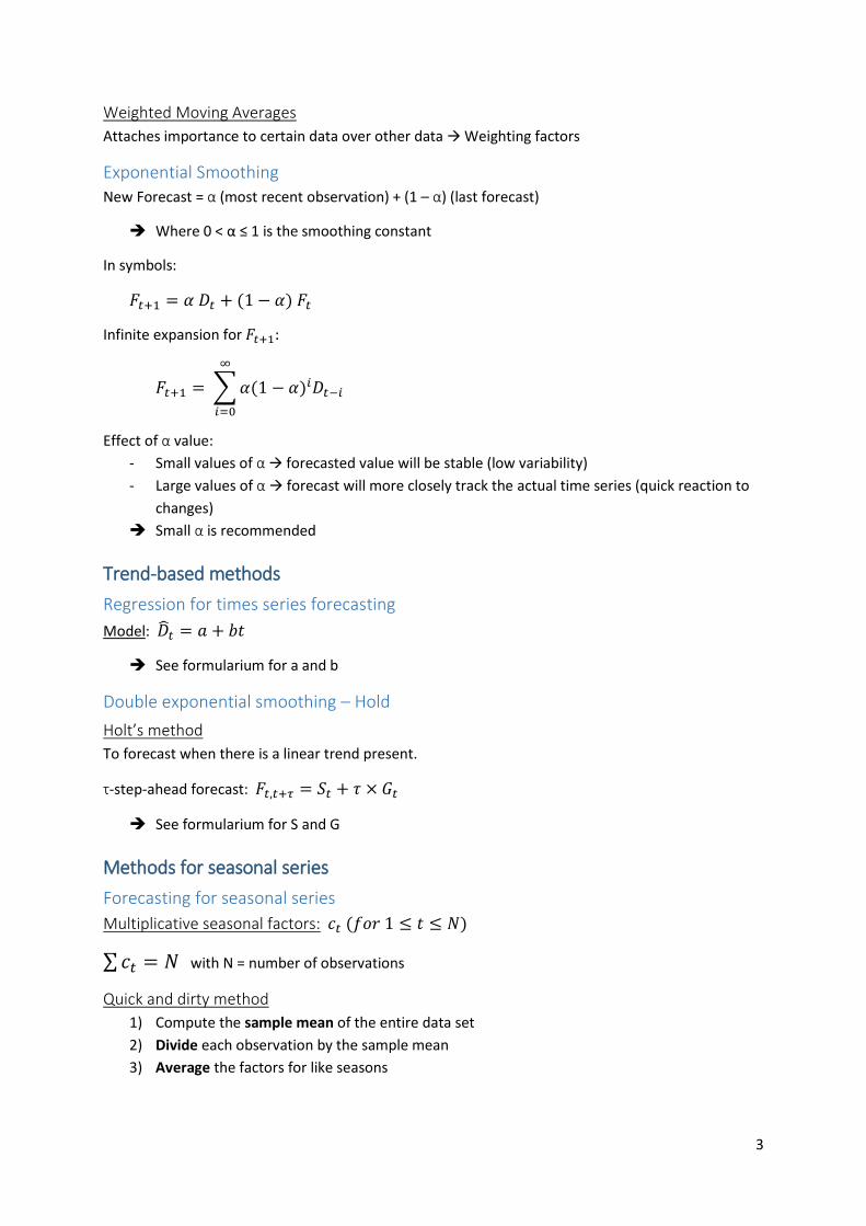
Weighted Moving Averages
Attaches importance to certain data over other data → Weighting factors
Exponential Smoothing
New Forecast = α (most recent observation) + (1 – α) (last forecast)
➔ Where 0 < α ≤ 1 is the smoothing constant
In symbols:
𝐹𝑡+1 = 𝛼 𝐷𝑡 + (1 − 𝛼) 𝐹𝑡
Infinite expansion for 𝐹𝑡+1:
𝐹𝑡+1 = ∑ 𝛼(1 − 𝛼)𝑖𝐷𝑡−𝑖
∞
𝑖=0
Effect of α value:
- Small values of α → forecasted value will be stable (low variability)
- Large values of α → forecast will more closely track the actual time series (quick reaction to
changes)
➔ Small α is recommended
Trend-based methods
Regression for times series forecasting
Model: �̂�𝑡 = 𝑎 + 𝑏𝑡
➔ See formularium for a and b
Double exponential smoothing – Hold
Holt’s method
To forecast when there is a linear trend present.
τ-step-ahead forecast: 𝐹𝑡,𝑡+𝜏 = 𝑆𝑡 + 𝜏 × 𝐺𝑡
➔ See formularium for S and G
Methods for seasonal series
Forecasting for seasonal series
Multiplicative seasonal factors: 𝑐𝑡 (𝑓𝑜𝑟 1 ≤ 𝑡 ≤ 𝑁)
∑ 𝑐𝑡 = 𝑁 with N = number of observations
Quick and dirty method
1) Compute the sample mean of the entire data set
2) Divide each observation by the sample mean
3) Average the factors for like seasons
4
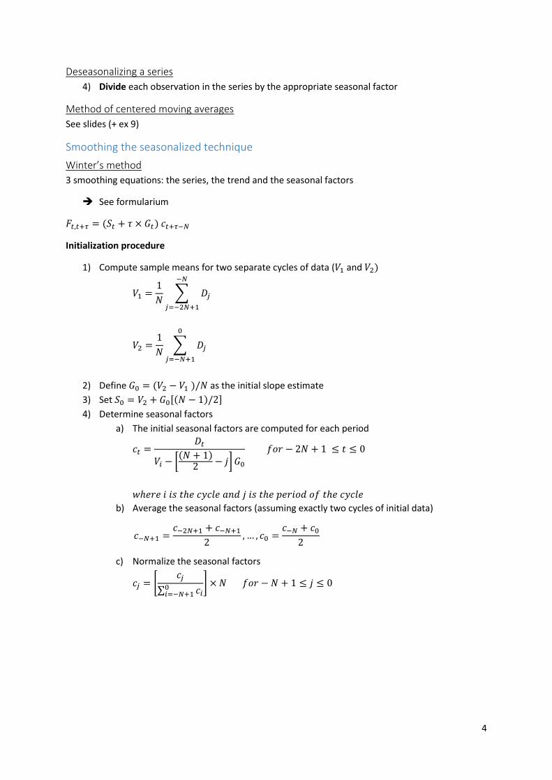
Deseasonalizing a series
4) Divide each observation in the series by the appropriate seasonal factor
Method of centered moving averages
See slides (+ ex 9)
Smoothing the seasonalized technique
Winter’s method
3 smoothing equations: the series, the trend and the seasonal factors
➔ See formularium
𝐹𝑡,𝑡+𝜏 = (𝑆𝑡 + 𝜏 × 𝐺𝑡) 𝑐𝑡+𝜏−𝑁
Initialization procedure
1) Compute sample means for two separate cycles of data (𝑉1 and 𝑉2)
𝑉1 =1
𝑁∑ 𝐷𝑗
−𝑁
𝑗=−2𝑁+1
𝑉2 =1
𝑁∑ 𝐷𝑗
0
𝑗=−𝑁+1
2) Define 𝐺0 = (𝑉2 − 𝑉1 )/𝑁 as the initial slope estimate
3) Set 𝑆0 = 𝑉2 + 𝐺0[(𝑁 − 1)/2]
4) Determine seasonal factors
a) The initial seasonal factors are computed for each period
𝑐𝑡 =𝐷𝑡
𝑉𝑖 − [(𝑁 + 1)
2 − 𝑗] 𝐺0
𝑓𝑜𝑟 − 2𝑁 + 1 ≤ 𝑡 ≤ 0
𝑤ℎ𝑒𝑟𝑒 𝑖 𝑖𝑠 𝑡ℎ𝑒 𝑐𝑦𝑐𝑙𝑒 𝑎𝑛𝑑 𝑗 𝑖𝑠 𝑡ℎ𝑒 𝑝𝑒𝑟𝑖𝑜𝑑 𝑜𝑓 𝑡ℎ𝑒 𝑐𝑦𝑐𝑙𝑒
b) Average the seasonal factors (assuming exactly two cycles of initial data)
𝑐−𝑁+1 =𝑐−2𝑁+1 + 𝑐−𝑁+1
2, … , 𝑐0 =
𝑐−𝑁 + 𝑐0
2
c) Normalize the seasonal factors
𝑐𝑗 = [𝑐𝑗
∑ 𝑐𝑖0𝑖=−𝑁+1
] × 𝑁 𝑓𝑜𝑟 − 𝑁 + 1 ≤ 𝑗 ≤ 0
5
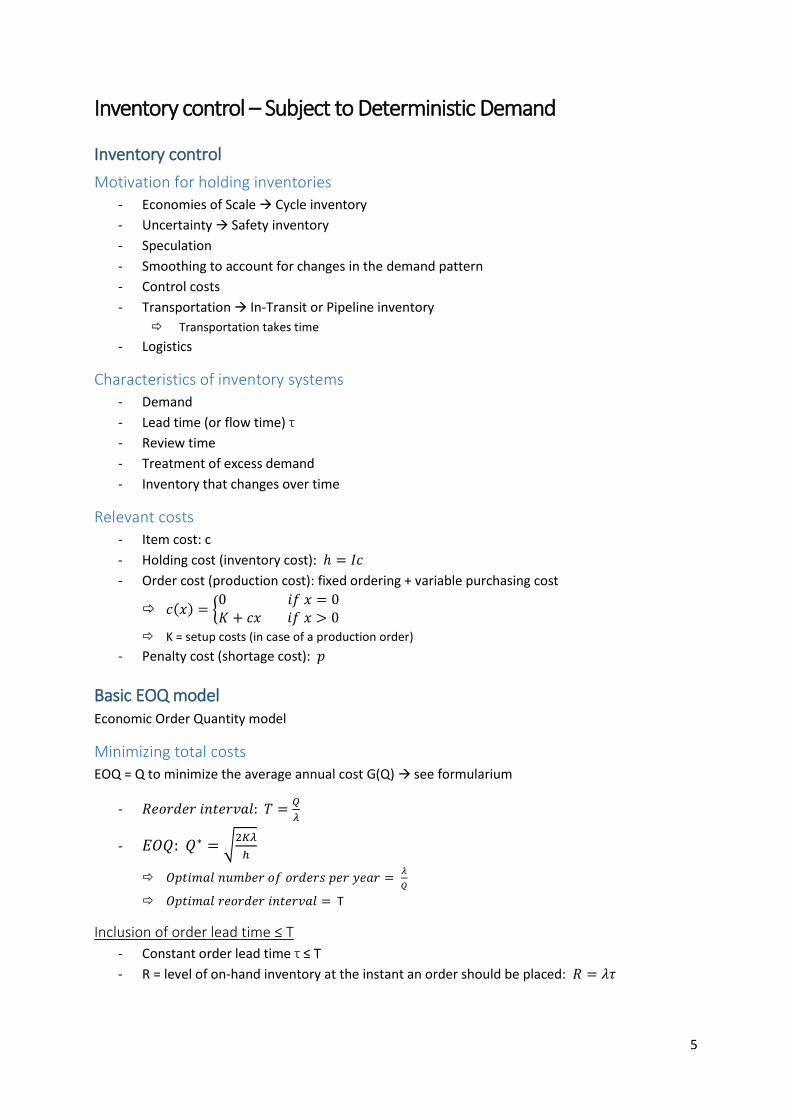
Inventory control – Subject to Deterministic Demand
Inventory control
Motivation for holding inventories
- Economies of Scale → Cycle inventory
- Uncertainty → Safety inventory
- Speculation
- Smoothing to account for changes in the demand pattern
- Control costs
- Transportation → In-Transit or Pipeline inventory
Transportation takes time
- Logistics
Characteristics of inventory systems
- Demand
- Lead time (or flow time) τ
- Review time
- Treatment of excess demand
- Inventory that changes over time
Relevant costs
- Item cost: c
- Holding cost (inventory cost): ℎ = 𝐼𝑐
- Order cost (production cost): fixed ordering + variable purchasing cost
𝑐(𝑥) = {0 𝑖𝑓 𝑥 = 0𝐾 + 𝑐𝑥 𝑖𝑓 𝑥 > 0
K = setup costs (in case of a production order)
- Penalty cost (shortage cost): 𝑝
Basic EOQ model Economic Order Quantity model
Minimizing total costs
EOQ = Q to minimize the average annual cost G(Q) → see formularium
- 𝑅𝑒𝑜𝑟𝑑𝑒𝑟 𝑖𝑛𝑡𝑒𝑟𝑣𝑎𝑙: 𝑇 =𝑄
𝜆
- 𝐸𝑂𝑄: 𝑄∗ = √2𝐾𝜆
ℎ
𝑂𝑝𝑡𝑖𝑚𝑎𝑙 𝑛𝑢𝑚𝑏𝑒𝑟 𝑜𝑓 𝑜𝑟𝑑𝑒𝑟𝑠 𝑝𝑒𝑟 𝑦𝑒𝑎𝑟 = 𝜆
𝑄
𝑂𝑝𝑡𝑖𝑚𝑎𝑙 𝑟𝑒𝑜𝑟𝑑𝑒𝑟 𝑖𝑛𝑡𝑒𝑟𝑣𝑎𝑙 = T
Inclusion of order lead time ≤ T
- Constant order lead time τ ≤ T
- R = level of on-hand inventory at the instant an order should be placed: 𝑅 = 𝜆𝜏
6
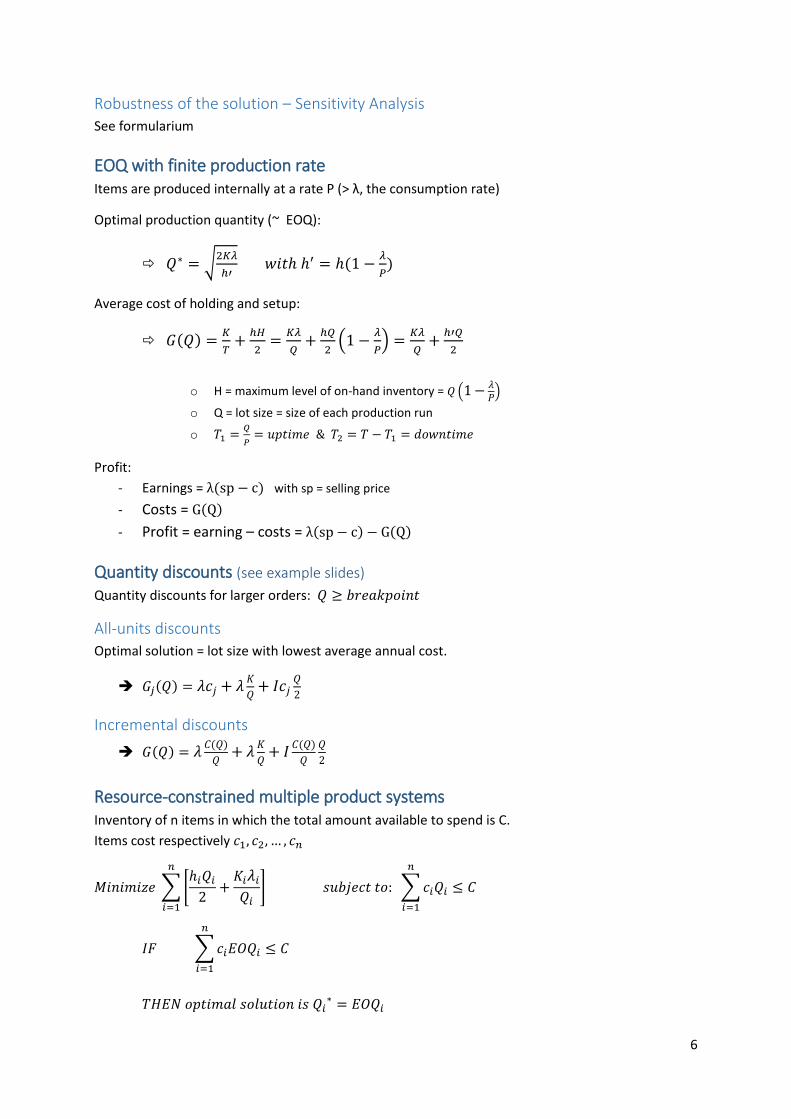
Robustness of the solution – Sensitivity Analysis
See formularium
EOQ with finite production rate Items are produced internally at a rate P (> λ, the consumption rate)
Optimal production quantity (~ EOQ):
𝑄∗ = √2𝐾𝜆
ℎ′ 𝑤𝑖𝑡ℎ ℎ′ = ℎ(1 −
𝜆
𝑃)
Average cost of holding and setup:
𝐺(𝑄) =𝐾
𝑇+
ℎ𝐻
2=
𝐾𝜆
𝑄+
ℎ𝑄
2(1 −
𝜆
𝑃) =
𝐾𝜆
𝑄+
ℎ′𝑄
2
o H = maximum level of on-hand inventory = 𝑄 (1 − 𝜆𝑃
)
o Q = lot size = size of each production run
o 𝑇1 =𝑄
𝑃= 𝑢𝑝𝑡𝑖𝑚𝑒 & 𝑇2 = 𝑇 − 𝑇1 = 𝑑𝑜𝑤𝑛𝑡𝑖𝑚𝑒
Profit:
- Earnings = λ(sp − c) with sp = selling price
- Costs = G(Q)
- Profit = earning – costs = λ(sp − c) − G(Q)
Quantity discounts (see example slides) Quantity discounts for larger orders: 𝑄 ≥ 𝑏𝑟𝑒𝑎𝑘𝑝𝑜𝑖𝑛𝑡
All-units discounts
Optimal solution = lot size with lowest average annual cost.
➔ 𝐺𝑗(𝑄) = 𝜆𝑐𝑗 + 𝜆𝐾
𝑄+ 𝐼𝑐𝑗
𝑄
2
Incremental discounts
➔ 𝐺(𝑄) = 𝜆𝐶(𝑄)
𝑄+ 𝜆
𝐾
𝑄+ 𝐼
𝐶(𝑄)
𝑄
𝑄
2
Resource-constrained multiple product systems Inventory of n items in which the total amount available to spend is C.
Items cost respectively 𝑐1, 𝑐2, … , 𝑐𝑛
𝑀𝑖𝑛𝑖𝑚𝑖𝑧𝑒 ∑ [ℎ𝑖𝑄𝑖
2+
𝐾𝑖𝜆𝑖
𝑄𝑖]
𝑛
𝑖=1
𝑠𝑢𝑏𝑗𝑒𝑐𝑡 𝑡𝑜: ∑ 𝑐𝑖𝑄𝑖 ≤ 𝐶
𝑛
𝑖=1
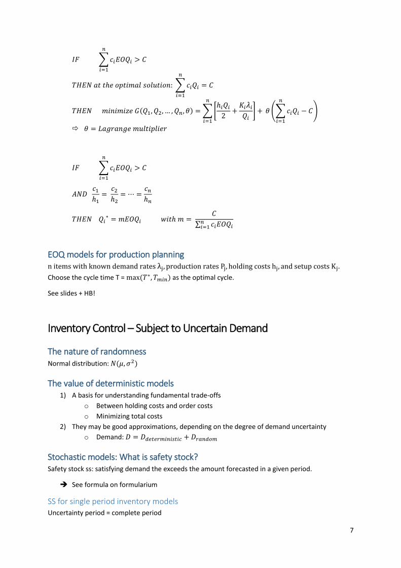
𝐼𝐹 ∑ 𝑐𝑖𝐸𝑂𝑄𝑖 ≤ 𝐶
𝑛
𝑖=1
𝑇𝐻𝐸𝑁 𝑜𝑝𝑡𝑖𝑚𝑎𝑙 𝑠𝑜𝑙𝑢𝑡𝑖𝑜𝑛 𝑖𝑠 𝑄𝑖∗ = 𝐸𝑂𝑄𝑖
7
𝐼𝐹 ∑ 𝑐𝑖𝐸𝑂𝑄𝑖 > 𝐶
𝑛
𝑖=1
𝑇𝐻𝐸𝑁 𝑎𝑡 𝑡ℎ𝑒 𝑜𝑝𝑡𝑖𝑚𝑎𝑙 𝑠𝑜𝑙𝑢𝑡𝑖𝑜𝑛: ∑ 𝑐𝑖𝑄𝑖 = 𝐶
𝑛
𝑖=1
𝑇𝐻𝐸𝑁 𝑚𝑖𝑛𝑖𝑚𝑖𝑧𝑒 𝐺(𝑄1, 𝑄2, … , 𝑄𝑛, 𝜃) = ∑ [ℎ𝑖𝑄𝑖
2+
𝐾𝑖𝜆𝑖
𝑄𝑖] +
𝑛
𝑖=1
𝜃 (∑ 𝑐𝑖𝑄𝑖 − 𝐶
𝑛
𝑖=1
)
𝜃 = 𝐿𝑎𝑔𝑟𝑎𝑛𝑔𝑒 𝑚𝑢𝑙𝑡𝑖𝑝𝑙𝑖𝑒𝑟
𝐼𝐹 ∑ 𝑐𝑖𝐸𝑂𝑄𝑖 > 𝐶
𝑛
𝑖=1
𝐴𝑁𝐷 𝑐1
ℎ1=
𝑐2
ℎ2= ⋯ =
𝑐𝑛
ℎ𝑛
𝑇𝐻𝐸𝑁 𝑄𝑖∗ = 𝑚𝐸𝑂𝑄𝑖 𝑤𝑖𝑡ℎ 𝑚 =
𝐶
∑ 𝑐𝑖𝐸𝑂𝑄𝑖𝑛𝑖=1
EOQ models for production planning n items with known demand rates λj, production rates Pj, holding costs hj, and setup costs Kj.
Choose the cycle time T = max (𝑇∗, 𝑇𝑚𝑖𝑛) as the optimal cycle.
See slides + HB!
Inventory Control – Subject to Uncertain Demand
The nature of randomness Normal distribution: 𝑁(𝜇, 𝜎2)
The value of deterministic models 1) A basis for understanding fundamental trade-offs
o Between holding costs and order costs
o Minimizing total costs
2) They may be good approximations, depending on the degree of demand uncertainty
o Demand: 𝐷 = 𝐷𝑑𝑒𝑡𝑒𝑟𝑚𝑖𝑛𝑖𝑠𝑡𝑖𝑐 + 𝐷𝑟𝑎𝑛𝑑𝑜𝑚
Stochastic models: What is safety stock? Safety stock ss: satisfying demand the exceeds the amount forecasted in a given period.
➔ See formula on formularium
SS for single period inventory models
Uncertainty period = complete period
8
SS for multiple period inventory models
Continuous review: (Q,R) policy
- Fixed order size Q, timing fluctuates
- Order at reorder point R
- Uncertainty period = lead time τ
Periodic review: (s,S) policy
- Fixed interval T, order quantity Q fluctuates
- Order up to inventory level S
- Uncertainty period = lead time τ + review period T
Lead time variability → see formularium
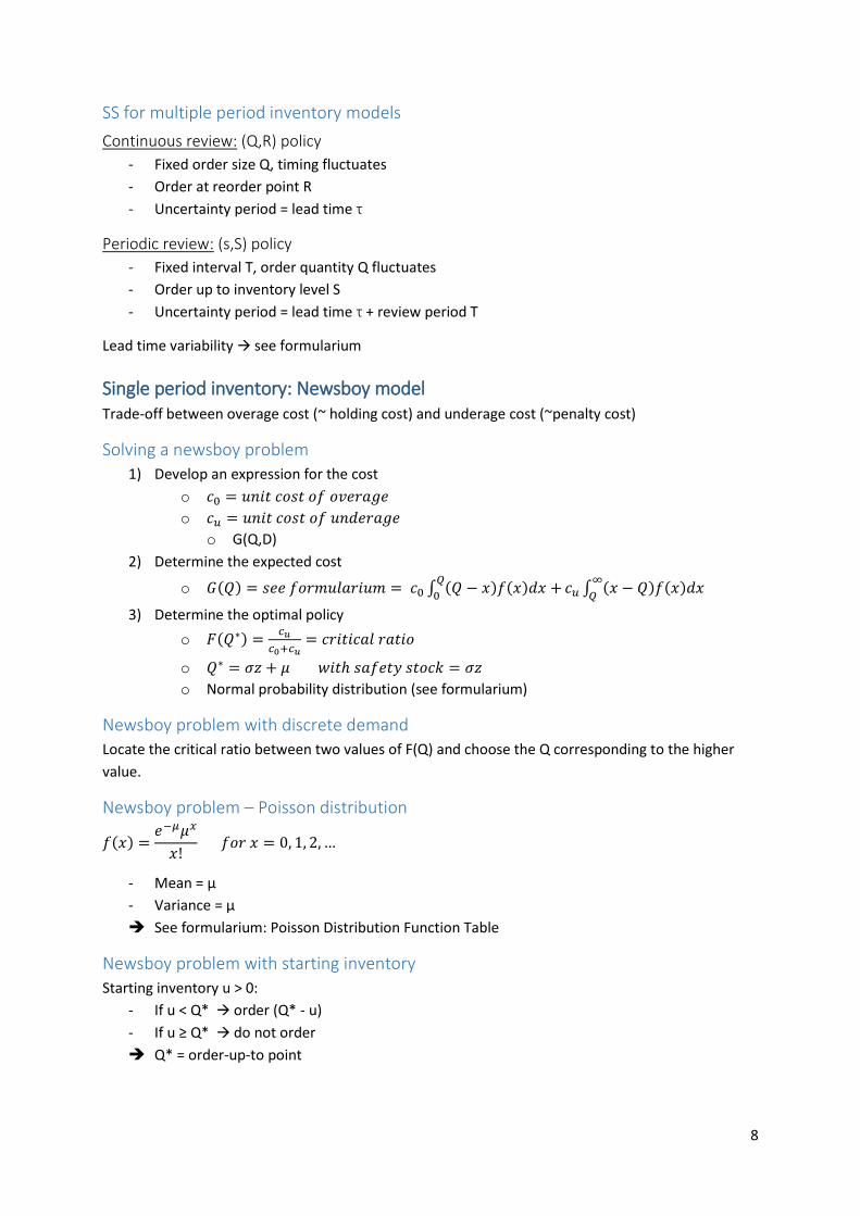
Single period inventory: Newsboy model Trade-off between overage cost (~ holding cost) and underage cost (~penalty cost)
Solving a newsboy problem
1) Develop an expression for the cost
o 𝑐0 = 𝑢𝑛𝑖𝑡 𝑐𝑜𝑠𝑡 𝑜𝑓 𝑜𝑣𝑒𝑟𝑎𝑔𝑒
o 𝑐𝑢 = 𝑢𝑛𝑖𝑡 𝑐𝑜𝑠𝑡 𝑜𝑓 𝑢𝑛𝑑𝑒𝑟𝑎𝑔𝑒
o G(Q,D)
2) Determine the expected cost
o 𝐺(𝑄) = 𝑠𝑒𝑒 𝑓𝑜𝑟𝑚𝑢𝑙𝑎𝑟𝑖𝑢𝑚 = 𝑐0 ∫ (𝑄 − 𝑥)𝑓(𝑥)𝑑𝑥 +𝑄
0𝑐𝑢 ∫ (𝑥 − 𝑄)𝑓(𝑥)𝑑𝑥
∞
𝑄
3) Determine the optimal policy
o 𝐹(𝑄∗) =𝑐𝑢
𝑐0+𝑐𝑢= 𝑐𝑟𝑖𝑡𝑖𝑐𝑎𝑙 𝑟𝑎𝑡𝑖𝑜
o 𝑄∗ = 𝜎𝑧 + 𝜇 𝑤𝑖𝑡ℎ 𝑠𝑎𝑓𝑒𝑡𝑦 𝑠𝑡𝑜𝑐𝑘 = 𝜎𝑧
o Normal probability distribution (see formularium)
Newsboy problem with discrete demand
Locate the critical ratio between two values of F(Q) and choose the Q corresponding to the higher
value.
Newsboy problem – Poisson distribution
𝑓(𝑥) =𝑒−𝜇𝜇𝑥
𝑥! 𝑓𝑜𝑟 𝑥 = 0, 1, 2, …
- Mean = μ
- Variance = μ
➔ See formularium: Poisson Distribution Function Table
Newsboy problem with starting inventory
Starting inventory u > 0:
- If u < Q* → order (Q* - u)
- If u ≥ Q* → do not order
➔ Q* = order-up-to point
9
Newsboy problem – Multiple planning periods
If all excess demand is back-ordered:
- 𝑐0 = holding cost
- 𝑐𝑢 = penalty cost (lost profit and/or loss-of-goodwill cost)
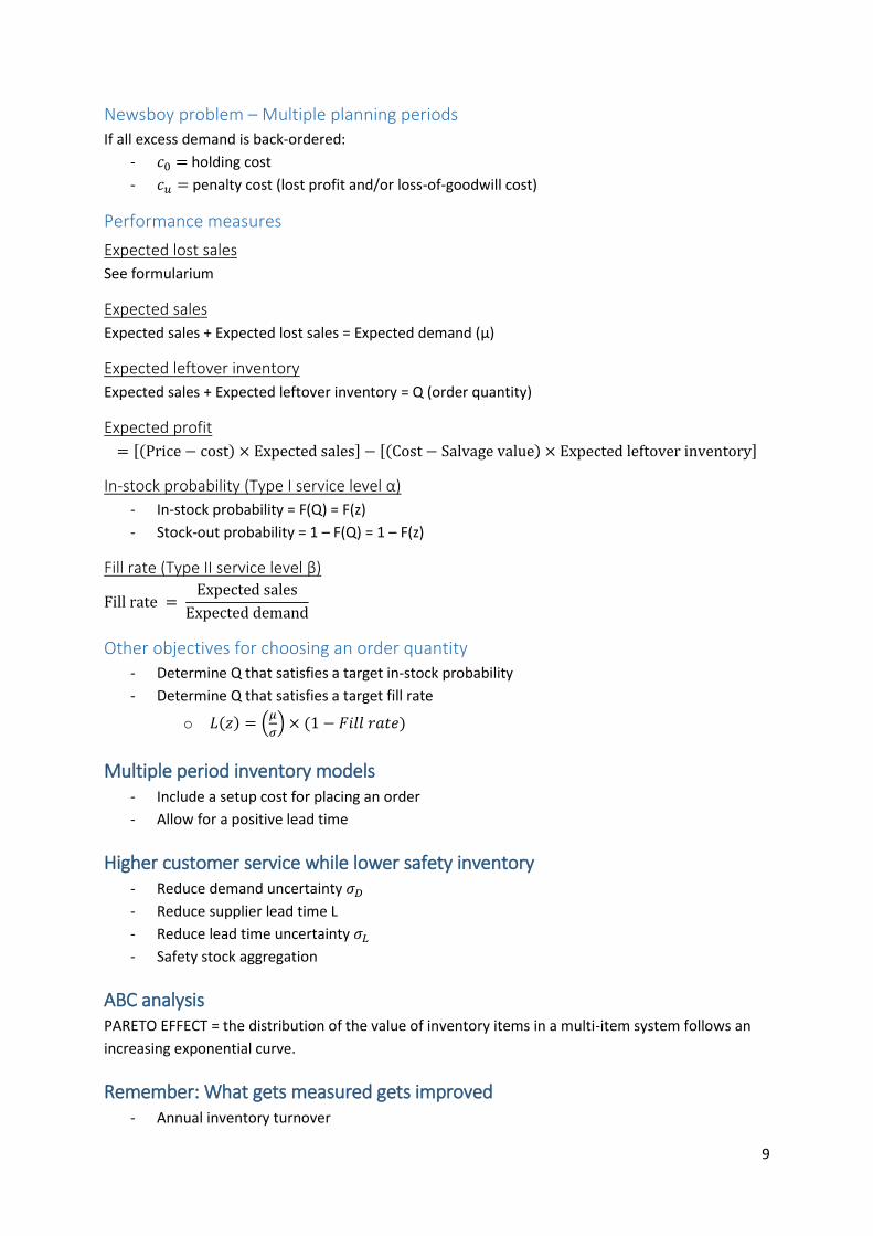
Performance measures
Expected lost sales
See formularium
Expected sales
Expected sales + Expected lost sales = Expected demand (μ)
Expected leftover inventory
Expected sales + Expected leftover inventory = Q (order quantity)
Expected profit
= [(Price − cost) × Expected sales] − [(Cost − Salvage value) × Expected leftover inventory]
In-stock probability (Type I service level α)
- In-stock probability = F(Q) = F(z)
- Stock-out probability = 1 – F(Q) = 1 – F(z)
Fill rate (Type II service level β)
Fill rate = Expected sales
Expected demand
Other objectives for choosing an order quantity
- Determine Q that satisfies a target in-stock probability
- Determine Q that satisfies a target fill rate
o 𝐿(𝑧) = (𝜇
𝜎) × (1 − 𝐹𝑖𝑙𝑙 𝑟𝑎𝑡𝑒)
Multiple period inventory models - Include a setup cost for placing an order
- Allow for a positive lead time
Higher customer service while lower safety inventory - Reduce demand uncertainty 𝜎𝐷
- Reduce supplier lead time L
- Reduce lead time uncertainty 𝜎𝐿
- Safety stock aggregation
ABC analysis PARETO EFFECT = the distribution of the value of inventory items in a multi-item system follows an
increasing exponential curve.
Remember: What gets measured gets improved - Annual inventory turnover
10
- Inventory holding period
- Inventory to assets ratio
- Customer service
Supply Chain Management
The role of information in the supply chain
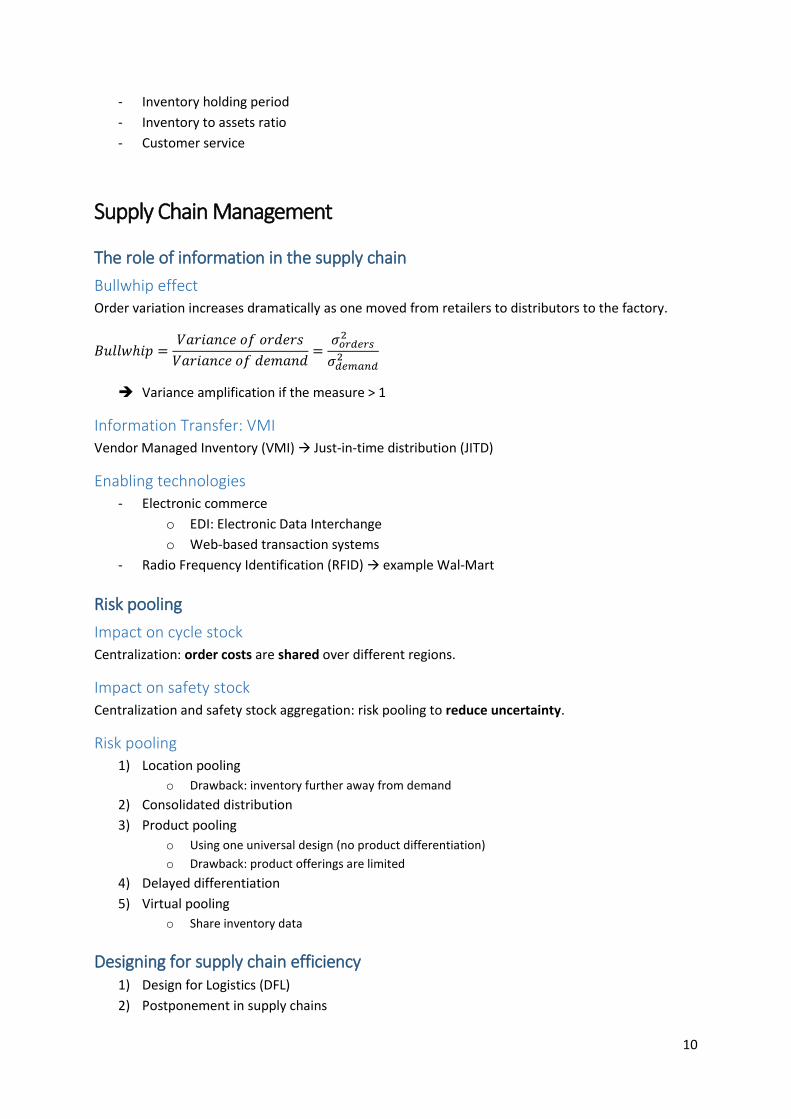
Bullwhip effect
Order variation increases dramatically as one moved from retailers to distributors to the factory.
𝐵𝑢𝑙𝑙𝑤ℎ𝑖𝑝 =𝑉𝑎𝑟𝑖𝑎𝑛𝑐𝑒 𝑜𝑓 𝑜𝑟𝑑𝑒𝑟𝑠
𝑉𝑎𝑟𝑖𝑎𝑛𝑐𝑒 𝑜𝑓 𝑑𝑒𝑚𝑎𝑛𝑑=
𝜎𝑜𝑟𝑑𝑒𝑟𝑠2
𝜎𝑑𝑒𝑚𝑎𝑛𝑑2
➔ Variance amplification if the measure > 1
Information Transfer: VMI
Vendor Managed Inventory (VMI) → Just-in-time distribution (JITD)
Enabling technologies
- Electronic commerce
o EDI: Electronic Data Interchange
o Web-based transaction systems
- Radio Frequency Identification (RFID) → example Wal-Mart
Risk pooling
Impact on cycle stock
Centralization: order costs are shared over different regions.
Impact on safety stock
Centralization and safety stock aggregation: risk pooling to reduce uncertainty.
Risk pooling
1) Location pooling
o Drawback: inventory further away from demand
2) Consolidated distribution
3) Product pooling
o Using one universal design (no product differentiation)
o Drawback: product offerings are limited
4) Delayed differentiation
5) Virtual pooling
o Share inventory data
Designing for supply chain efficiency 1) Design for Logistics (DFL)
2) Postponement in supply chains
11
o Postponing the final configuration of the product until the last possible point.
3) Configuration of the supplier base
o Streamlining the supply chain: reducing the number and variety of suppliers.
4) Outsourcing arrangements
5) Channels of distribution → Intermediate storage locations
Management of waiting lines
Waiting lines Queuing theory = mathematical approach to the analysis of waiting lines.
Why is there waiting?
- Variability
- Mismatch between supply and demand
Waiting line management Goal: Minimize Total cost = Customer waiting cost + Capacity cost
Characteristics of waiting lines
Population source
- Infinite-source situation
- Finite-source situation
Number of servers (channels)
- Single- vs multiple-channel
- Single- vs multiple phase
Arrival and service patterns
- Customer service times → (negative) exponential distribution
- Customer arrivals per unit of time → Poisson distribution
We assume customers are patient.
Other possibilities:
- Reneging: leave the line
- Jockeying: switch to another line
- Balking: not enter the line
Queue discipline (order of service)
- First-come, first-served (fcfs)
- Other priority rules
Queuing models: infinite source
Notation and basic relationships
𝜆 = 𝑐𝑢𝑠𝑡𝑜𝑚𝑒𝑟 𝑎𝑟𝑟𝑖𝑣𝑎𝑙 𝑟𝑎𝑡𝑒
𝜇 = 𝑠𝑒𝑟𝑣𝑖𝑐𝑒 𝑟𝑎𝑡𝑒 𝑝𝑒𝑟 𝑠𝑒𝑟𝑣𝑒𝑟
12
➔ 𝐴𝑣𝑒𝑟𝑎𝑔𝑒 𝑛𝑢𝑚𝑏𝑒𝑟 𝑜𝑓 𝑐𝑢𝑠𝑡𝑜𝑚𝑒𝑟𝑠 𝑏𝑒𝑖𝑛𝑔 𝑠𝑒𝑟𝑣𝑒𝑑: 𝑟 =𝜆
𝜇
𝐿𝑞 = 𝑎𝑣𝑒𝑟𝑎𝑔𝑒 𝑛𝑢𝑚𝑏𝑒𝑟 𝑜𝑓 𝑐𝑢𝑠𝑡𝑜𝑚𝑒𝑟𝑠 𝑤𝑎𝑖𝑡𝑖𝑛𝑔 𝑓𝑜𝑟 𝑠𝑒𝑟𝑣𝑖𝑐𝑒
𝐿𝑠 = 𝑎𝑣𝑒𝑟𝑎𝑔𝑒 𝑛𝑢𝑚𝑏𝑒𝑟 𝑜𝑓 𝑐𝑢𝑠𝑡𝑜𝑚𝑒𝑟𝑠 𝑖𝑛 𝑡ℎ𝑒 𝑠𝑦𝑠𝑡𝑒𝑚 (𝑤𝑎𝑖𝑡𝑖𝑛𝑔 𝑎𝑛𝑑 𝑜𝑟⁄ 𝑏𝑒𝑖𝑛𝑔 𝑠𝑒𝑟𝑣𝑒𝑑)
➔ 𝐴𝑣𝑒𝑟𝑎𝑔𝑒 𝑛𝑢𝑚𝑏𝑒𝑟 𝑜𝑓 𝑐𝑢𝑠𝑡𝑜𝑚𝑒𝑟𝑠: 𝐿𝑠 = 𝐿𝑞 + 𝑟
𝑊𝑞 = 𝑎𝑣𝑒𝑟𝑎𝑔𝑒 𝑡𝑖𝑚𝑒 𝑐𝑢𝑠𝑡𝑜𝑚𝑒𝑟𝑠 𝑤𝑎𝑖𝑡 𝑖𝑛 𝑙𝑖𝑛𝑒
𝑊𝑠 = 𝑎𝑣𝑒𝑟𝑎𝑔𝑒 𝑡𝑖𝑚𝑒 𝑐𝑢𝑠𝑡𝑜𝑚𝑒𝑟𝑠 𝑠𝑝𝑒𝑛𝑑 𝑖𝑛 𝑡ℎ𝑒 𝑠𝑦𝑠𝑡𝑒𝑚 (𝑤𝑎𝑖𝑡𝑖𝑛𝑔 𝑖𝑛 𝑙𝑖𝑛𝑒 𝑎𝑛𝑑 𝑠𝑒𝑟𝑣𝑖𝑐𝑒 𝑡𝑖𝑚𝑒)
➔ 𝐿𝑖𝑡𝑡𝑙𝑒′𝑠 𝑙𝑎𝑤: 𝐿𝑠 = 𝜆𝑊𝑠 𝑎𝑛𝑑 𝐿𝑞 = 𝜆𝑊𝑞
𝜌 = 𝑡ℎ𝑒 𝑠𝑦𝑠𝑡𝑒𝑚 𝑢𝑡𝑖𝑙𝑖𝑧𝑎𝑡𝑖𝑜𝑛 → 𝑠𝑒𝑒 𝑓𝑜𝑟𝑚𝑢𝑙𝑎𝑟𝑖𝑢𝑚
1
𝜇= 𝑠𝑒𝑟𝑣𝑖𝑐𝑒 𝑡𝑖𝑚𝑒
➔ 𝑊𝑠 = 𝑊𝑞 + 𝑟
𝑀 = 𝑛𝑢𝑚𝑏𝑒𝑟 𝑜𝑓 𝑠𝑒𝑟𝑣𝑒𝑟𝑠
𝑃0 = 𝑝𝑟𝑜𝑏𝑎𝑏𝑖𝑙𝑖𝑡𝑦 𝑜𝑓 𝑧𝑒𝑟𝑜 𝑢𝑛𝑖𝑡𝑠 𝑖𝑛 𝑡ℎ𝑒 𝑠𝑦𝑠𝑡𝑒𝑚
𝑃𝑛 = 𝑝𝑟𝑜𝑏𝑎𝑏𝑖𝑙𝑖𝑡𝑦 𝑜𝑓 𝑛 𝑢𝑛𝑖𝑡𝑠 𝑖𝑛 𝑡ℎ𝑒 𝑠𝑦𝑠𝑡𝑒𝑚
𝐿𝑚𝑎𝑥 = 𝑚𝑎𝑥𝑖𝑚𝑢𝑚 𝑒𝑥𝑝𝑒𝑐𝑡𝑒𝑑 𝑛𝑢𝑚𝑏𝑒𝑟 𝑜𝑓 𝑐𝑢𝑠𝑡𝑜𝑚𝑒𝑟𝑠 𝑤𝑎𝑖𝑡𝑖𝑛𝑔 𝑖𝑛 𝑙𝑖𝑛𝑒
Assumptions
- System operating under steady-state conditions: average arrival and service rates are stable.
- No limit on the length of the queue.
Kendall’s notation: A/B/C
- A: Distribution of inter-arrival times of customers (time between arrivals to the queue)
- B: Distribution of service times
- C: Number of servers
➔ M: Exponential Distribution (Markovian)
➔ D: Deterministic Distribution
M/M/1 infinite-source fcfs queuing model
See formularium
M/D/1 infinite-source fcfs queuing model
Effect of constant service time:
- Cut in half the average number of customer waiting in line (𝐿𝑞)
- Cut in half the average customers spend waiting in line (𝑊𝑞)
Automatically done because 𝐿𝑞 is already cut in half!
➔ Elimination or reduction of the variability: shortening of waiting lines
13
M/M/S infinite-source fcfs queuing model
Assumptions
- Servers all work at the same average rate → number of servers = S
- Customers form a single waiting line
Notations
𝑊𝑎 = 𝑎𝑣𝑒𝑟𝑎𝑔𝑒 𝑤𝑎𝑖𝑡𝑖𝑛𝑔 𝑡𝑖𝑚𝑒 𝑓𝑜𝑟 𝑎𝑛 𝑎𝑟𝑟𝑖𝑣𝑎𝑙 𝑛𝑜𝑡 𝑖𝑚𝑚𝑒𝑑𝑖𝑎𝑡𝑒𝑙𝑦 𝑠𝑒𝑟𝑣𝑒𝑑
𝑃𝑤 = 𝑝𝑟𝑜𝑏𝑎𝑏𝑖𝑙𝑖𝑡𝑦 𝑡ℎ𝑎𝑡 𝑎𝑛 𝑎𝑟𝑟𝑖𝑣𝑎𝑙 𝑤𝑖𝑙𝑙 ℎ𝑎𝑣𝑒 𝑡𝑜 𝑤𝑎𝑖𝑡 𝑓𝑜𝑟 𝑠𝑒𝑟𝑣𝑖𝑐𝑒
Table for values of 𝐿𝑞 and 𝑃0
➔ See formularium
Maximum line length
Determine the approximate line length n that will satisfy a specified percentage.
➔ See formularium for n
M/M/S multiple-priority model
Assumptions
- Arriving customers are assigned to priority classes
- Highest class first, within each class: first-come, first-served
- Revising priorities is possible
Notations
𝑊𝑘 = 𝑎𝑣𝑒𝑟𝑎𝑔𝑒 𝑤𝑎𝑖𝑡𝑖𝑛𝑔 𝑡𝑖𝑚𝑒 𝑖𝑛 𝑙𝑖𝑛𝑒 𝑓𝑜𝑟 𝑢𝑛𝑖𝑡𝑠 𝑖𝑛 𝑘𝑡ℎ 𝑝𝑟𝑖𝑜𝑟𝑖𝑡𝑦 𝑐𝑙𝑎𝑠𝑠
𝑊 = 𝑎𝑣𝑒𝑟𝑎𝑔𝑒 𝑡𝑖𝑚𝑒 𝑖𝑛 𝑡ℎ𝑒 𝑠𝑦𝑠𝑡𝑒𝑚 𝑓𝑜𝑟 𝑢𝑛𝑖𝑡𝑠 𝑖𝑛 𝑡ℎ𝑒 𝑘𝑡ℎ 𝑝𝑟𝑖𝑜𝑟𝑖𝑡𝑦 𝑐𝑙𝑎𝑠𝑠
𝐿𝑘 = 𝑎𝑣𝑒𝑟𝑎𝑔𝑒 𝑛𝑢𝑚𝑏𝑒𝑟 𝑤𝑎𝑖𝑡𝑖𝑛𝑔 𝑖𝑛 𝑙𝑖𝑛𝑒 𝑓𝑜𝑟 𝑢𝑛𝑖𝑡𝑠 𝑖𝑛 𝑘𝑡ℎ 𝑝𝑟𝑖𝑜𝑟𝑖𝑡𝑦 𝑐𝑙𝑎𝑠𝑠
➔ See formularium
Queuing models: finite source
Assumptions
- Arrival rates → Poisson
- Service times → Exponential
See formularium
Downtime = Waiting time + Service time
Probability of not waiting = 1 – Probability of waiting
Cost analysis Designing systems that achieve a balance between (service) capacity and customer waiting time.
Other solutions:
- Reduce variability
- Reduce the cost of waiting

14
o Reduce perceived waiting time (as opposed to actual waiting time)
o Derive benefit from customer waiting
15
Simulation
Basic steps for all simulation models 1) Identify the problem and set objectives.
2) Develop the simulation model.
3) Test the model to be sure that it reflects the system being studied = VALIDATION
4) Develop one or more experiments.
5) Run the simulation and evaluate results.
6) Repeat step 4 and 5 until satisfied.
Monte Carlo simulation Random sampling from probability distributions.
1) Identify a probability distribution for each random component of the system.
2) Work out an assignment so that intervals of random numbers will correspond to the
probability distribution.
3) Obtain the random numbers needed for the study: computer generated or tables.
4) Interpret the results.
Simulating theoretical distributions
- Poisson:
Obtain discrete cumulative distribution from a table
- Normal:
𝑆𝑖𝑚𝑢𝑙𝑎𝑡𝑒𝑑 𝑣𝑎𝑙𝑢𝑒 = 𝜇 + (𝑅𝑎𝑛𝑑𝑜𝑚 𝑛𝑢𝑚𝑏𝑒𝑟 × 𝜎)
- Uniform distribution:
𝑆𝑖𝑚𝑢𝑙𝑎𝑡𝑒𝑑 𝑣𝑎𝑙𝑢𝑒 = 𝑎 + (𝑏 − 𝑎)(𝑅𝑎𝑛𝑑𝑜𝑚 𝑛𝑢𝑚𝑏𝑒𝑟 𝑎𝑠 𝑎 𝑝𝑒𝑟𝑐𝑒𝑛𝑡𝑎𝑔𝑒)
- Negative Exponential Distribution :
𝑃(𝑡 ≥ 𝑇) = 𝑒−𝜆𝑡 𝑎𝑛𝑑 𝑃(𝑡 ≥ 𝑇) = 𝑅𝑎𝑛𝑑𝑜𝑚 𝑛𝑢𝑚𝑏𝑒𝑟
𝑡 = −ln (𝑅𝑎𝑛𝑑𝑜𝑚 𝑛𝑢𝑚𝑏𝑒𝑟)
𝜆
Discrete-event simulation Discrete-event simulation (DES) models the operation of a system as a discrete sequence of events in
time.
- Each event → change of state
- Between consecutive events → no change assumed
➔ Simulation jumps in time
Limitations - No optimum solution
- Approximate behavior
- Large-scale simulation requires considerable effort
Decision-making process See slide 29
16
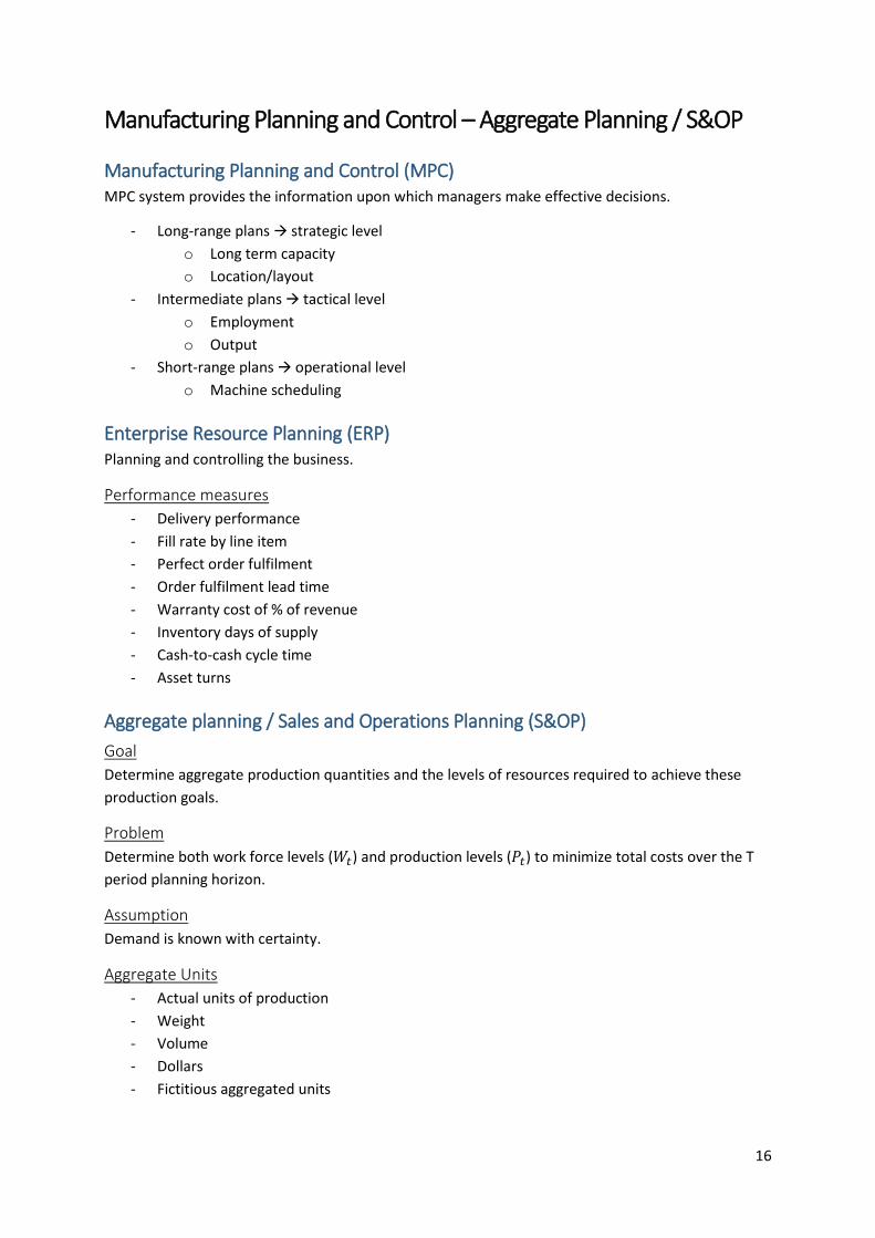
Manufacturing Planning and Control – Aggregate Planning / S&OP
Manufacturing Planning and Control (MPC) MPC system provides the information upon which managers make effective decisions.
- Long-range plans → strategic level
o Long term capacity
o Location/layout
- Intermediate plans → tactical level
o Employment
o Output
- Short-range plans → operational level
o Machine scheduling
Enterprise Resource Planning (ERP) Planning and controlling the business.
Performance measures
- Delivery performance
- Fill rate by line item
- Perfect order fulfilment
- Order fulfilment lead time
- Warranty cost of % of revenue
- Inventory days of supply
- Cash-to-cash cycle time
- Asset turns
Aggregate planning / Sales and Operations Planning (S&OP)
Goal
Determine aggregate production quantities and the levels of resources required to achieve these
production goals.
Problem
Determine both work force levels (𝑊𝑡) and production levels (𝑃𝑡) to minimize total costs over the T
period planning horizon.
Assumption
Demand is known with certainty.
Aggregate Units
- Actual units of production
- Weight
- Volume
- Dollars
- Fictitious aggregated units
17
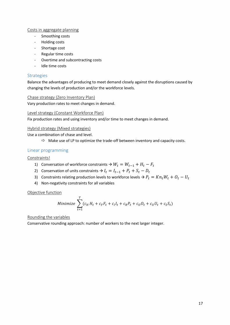
Costs in aggregate planning
- Smoothing costs
- Holding costs
- Shortage cost
- Regular time costs
- Overtime and subcontracting costs
- Idle time costs
Strategies
Balance the advantages of producing to meet demand closely against the disruptions caused by
changing the levels of production and/or the workforce levels.
Chase strategy (Zero Inventory Plan)
Vary production rates to meet changes in demand.
Level strategy (Constant Workforce Plan)
Fix production rates and using inventory and/or time to meet changes in demand.
Hybrid strategy (Mixed strategies)
Use a combination of chase and level.
Make use of LP to optimize the trade-off between inventory and capacity costs.
Linear programming
Constraints!
1) Conversation of workforce constraints → 𝑊𝑡 = 𝑊𝑡−1 + 𝐻𝑡 − 𝐹𝑡
2) Conservation of units constraints → 𝐼𝑡 = 𝐼𝑡−1 + 𝑃𝑡 + 𝑆𝑡 − 𝐷𝑡
3) Constraints relating production levels to workforce levels → 𝑃𝑡 = 𝐾𝑛𝑡𝑊𝑡 + 𝑂𝑡 − 𝑈𝑡
4) Non-negativity constraints for all variables
Objective function
𝑀𝑖𝑛𝑖𝑚𝑖𝑧𝑒 ∑(𝑐𝐻
𝑇
𝑡=1
𝐻𝑡 + 𝑐𝐹𝐹𝑡 + 𝑐𝐼𝐼𝑡 + 𝑐𝑅𝑃𝑡 + 𝑐𝑂𝑂𝑡 + 𝑐𝑈𝑈𝑡 + 𝑐𝑆𝑆𝑡)
Rounding the variables
Conservative rounding approach: number of workers to the next larger integer.
18
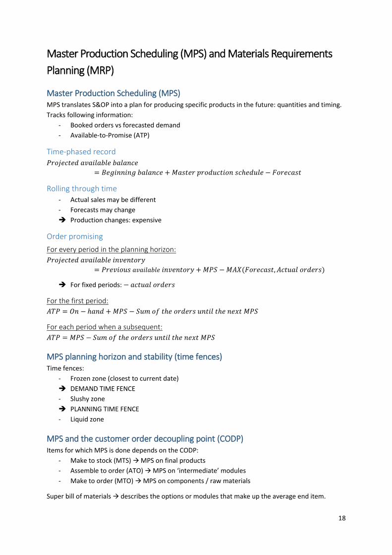
Master Production Scheduling (MPS) and Materials Requirements
Planning (MRP)
Master Production Scheduling (MPS) MPS translates S&OP into a plan for producing specific products in the future: quantities and timing.
Tracks following information:
- Booked orders vs forecasted demand
- Available-to-Promise (ATP)
Time-phased record
𝑃𝑟𝑜𝑗𝑒𝑐𝑡𝑒𝑑 𝑎𝑣𝑎𝑖𝑙𝑎𝑏𝑙𝑒 𝑏𝑎𝑙𝑎𝑛𝑐𝑒
= 𝐵𝑒𝑔𝑖𝑛𝑛𝑖𝑛𝑔 𝑏𝑎𝑙𝑎𝑛𝑐𝑒 + 𝑀𝑎𝑠𝑡𝑒𝑟 𝑝𝑟𝑜𝑑𝑢𝑐𝑡𝑖𝑜𝑛 𝑠𝑐ℎ𝑒𝑑𝑢𝑙𝑒 − 𝐹𝑜𝑟𝑒𝑐𝑎𝑠𝑡
Rolling through time
- Actual sales may be different
- Forecasts may change
➔ Production changes: expensive
Order promising
For every period in the planning horizon:
𝑃𝑟𝑜𝑗𝑒𝑐𝑡𝑒𝑑 𝑎𝑣𝑎𝑖𝑙𝑎𝑏𝑙𝑒 𝑖𝑛𝑣𝑒𝑛𝑡𝑜𝑟𝑦
= 𝑃𝑟𝑒𝑣𝑖𝑜𝑢𝑠 𝑎𝑣𝑎𝑖𝑙𝑎𝑏𝑙𝑒 𝑖𝑛𝑣𝑒𝑛𝑡𝑜𝑟𝑦 + 𝑀𝑃𝑆 − 𝑀𝐴𝑋(𝐹𝑜𝑟𝑒𝑐𝑎𝑠𝑡, 𝐴𝑐𝑡𝑢𝑎𝑙 𝑜𝑟𝑑𝑒𝑟𝑠)
➔ For fixed periods: − 𝑎𝑐𝑡𝑢𝑎𝑙 𝑜𝑟𝑑𝑒𝑟𝑠
For the first period:
𝐴𝑇𝑃 = 𝑂𝑛 − ℎ𝑎𝑛𝑑 + 𝑀𝑃𝑆 − 𝑆𝑢𝑚 𝑜𝑓 𝑡ℎ𝑒 𝑜𝑟𝑑𝑒𝑟𝑠 𝑢𝑛𝑡𝑖𝑙 𝑡ℎ𝑒 𝑛𝑒𝑥𝑡 𝑀𝑃𝑆
For each period when a subsequent:
𝐴𝑇𝑃 = 𝑀𝑃𝑆 − 𝑆𝑢𝑚 𝑜𝑓 𝑡ℎ𝑒 𝑜𝑟𝑑𝑒𝑟𝑠 𝑢𝑛𝑡𝑖𝑙 𝑡ℎ𝑒 𝑛𝑒𝑥𝑡 𝑀𝑃𝑆
MPS planning horizon and stability (time fences) Time fences:
- Frozen zone (closest to current date)
➔ DEMAND TIME FENCE
- Slushy zone
➔ PLANNING TIME FENCE
- Liquid zone
MPS and the customer order decoupling point (CODP) Items for which MPS is done depends on the CODP:
- Make to stock (MTS) → MPS on final products
- Assemble to order (ATO) → MPS on ‘intermediate’ modules
- Make to order (MTO) → MPS on components / raw materials
Super bill of materials → describes the options or modules that make up the average end item.
19
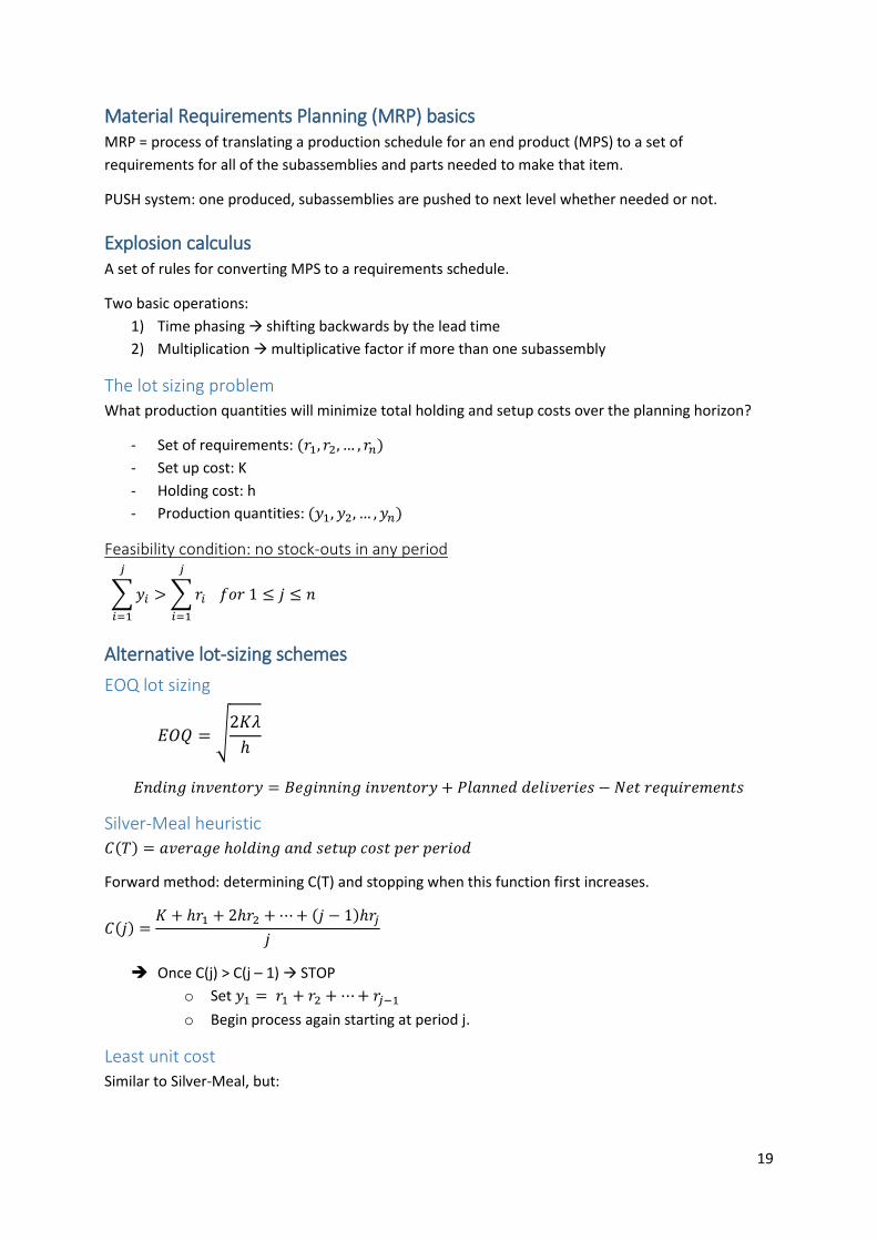
Material Requirements Planning (MRP) basics MRP = process of translating a production schedule for an end product (MPS) to a set of
requirements for all of the subassemblies and parts needed to make that item.
PUSH system: one produced, subassemblies are pushed to next level whether needed or not.
Explosion calculus A set of rules for converting MPS to a requirements schedule.
Two basic operations:
1) Time phasing → shifting backwards by the lead time
2) Multiplication → multiplicative factor if more than one subassembly
The lot sizing problem
What production quantities will minimize total holding and setup costs over the planning horizon?
- Set of requirements: (𝑟1, 𝑟2, … , 𝑟𝑛)
- Set up cost: K
- Holding cost: h
- Production quantities: (𝑦1, 𝑦2, … , 𝑦𝑛)
Feasibility condition: no stock-outs in any period
∑ 𝑦𝑖
𝑗
𝑖=1
> ∑ 𝑟𝑖
𝑗
𝑖=1
𝑓𝑜𝑟 1 ≤ 𝑗 ≤ 𝑛
Alternative lot-sizing schemes
EOQ lot sizing
𝐸𝑂𝑄 = √2𝐾𝜆
ℎ
𝐸𝑛𝑑𝑖𝑛𝑔 𝑖𝑛𝑣𝑒𝑛𝑡𝑜𝑟𝑦 = 𝐵𝑒𝑔𝑖𝑛𝑛𝑖𝑛𝑔 𝑖𝑛𝑣𝑒𝑛𝑡𝑜𝑟𝑦 + 𝑃𝑙𝑎𝑛𝑛𝑒𝑑 𝑑𝑒𝑙𝑖𝑣𝑒𝑟𝑖𝑒𝑠 − 𝑁𝑒𝑡 𝑟𝑒𝑞𝑢𝑖𝑟𝑒𝑚𝑒𝑛𝑡𝑠
Silver-Meal heuristic
𝐶(𝑇) = 𝑎𝑣𝑒𝑟𝑎𝑔𝑒 ℎ𝑜𝑙𝑑𝑖𝑛𝑔 𝑎𝑛𝑑 𝑠𝑒𝑡𝑢𝑝 𝑐𝑜𝑠𝑡 𝑝𝑒𝑟 𝑝𝑒𝑟𝑖𝑜𝑑
Forward method: determining C(T) and stopping when this function first increases.
𝐶(𝑗) =𝐾 + ℎ𝑟1 + 2ℎ𝑟2 + ⋯ + (𝑗 − 1)ℎ𝑟𝑗
𝑗
➔ Once C(j) > C(j – 1) → STOP
o Set 𝑦1 = 𝑟1 + 𝑟2 + ⋯ + 𝑟𝑗−1
o Begin process again starting at period j.
Least unit cost
Similar to Silver-Meal, but:
20
𝐶(𝑗) =𝐾 + ℎ𝑟1 + 2ℎ𝑟2 + ⋯ + (𝑗 − 1)ℎ𝑟𝑗
(𝑟1 + 𝑟2 + ⋯ + 𝑟𝑗−1)
Part period balancing
Set the order horizon equal to the number of periods that most closely matches the total holding cost
with the setup cost over that period.
Lot sizing with capacity constraints
Detecting an infeasible problem
An infeasible problem: r = (52, 87, 23, 56) and c = (60, 60, 60, 60)
Obtaining a feasible solution for a feasible problem
A feasible problem: r = (20, 40, 100, 35, 80, 75, 25) and c = (60, 60, 60, 60, 60, 60, 60)
➔ Approximate lot-shifting technique: back-shift demand to prior periods
Improving a feasible solution
By shifting, starting from the last period and working backward to the beginning.
Shortcomings of MRP - Uncertainty
- Capacity planning
- Rolling horizons and system nervousness
- Lead times dependent on lot sizes
- Quality problems
- Data integrity
- Order pegging
Just-in-time and Kanban
Push and Pull Push systems: schedule release of work based on information from outside the system.
Actual or forecasted demand
Due date drive
Do not limit WIP
Pull systems: authorize release of work based on information from inside the system.
System status
Rate driven
Limit on WIP
Kanban Kanban is a mechanism for implementing pull.
All goods must be accompanied by a Kanban (card).
Kanban cards help create a demand-driven system.
21
Types:
- Conveyance/transportation Kanban
- Production Kanban
- Sales/vendor Kanban
How many Kanban cards needed in 1 loop?
See formularium
Lead time: processing time + waiting time + conveyance time
Setting number of Kanban cards = maximum inventory
Kanban card count for multiple products
Take into account:
- Changeover times
- Minimum batch sizes
- Takt time: amount of time that must elapse between two consecutive unit completions in
order to meet the demand.
Setting minimum batch sizes (MBS)
MBS = minimum number of cards → low water level (<-> high water)
Number must be rounded up (for feasibility) to an integer number of Kanbans
Comparison of MRP and JIT
MRP: push system
- Based on forecasts of sales of end items.
- Once produced, subassemblies are pushed to next level whether needed or not.
JIT: pull system
- Production at one level only happens when initiated by a request at the higher level.
- Unit are pulled through the system by request.
Setup time reduction – SMED
Definition of setup Setup or changeover = preparation and after-adjustment before and after each lot is processed.
Why setup time reduction? - Economic lot size
- Changing market conditions
Changing market demands: need for diversified, low-volume production.
Frequent setups necessary to produce a variety of goods in small lots.
- Benefits:
o Increased flexibility
o Increased bottleneck capacity
o Reduced costs
22
What is SMED? Single-Minute Exchange of Die
A theory and techniques for performing setup operations in under ten minutes.
History of SMED Shigeo Shingo
Two different types of setup operations:
1) Internal setup (IED: inner exchange of die)
Can only be performed when the machine is stopped
2) External setup (OED: outer exchange of die)
Can be performed while machine is in operation
Fundamentals of SMED 1) Preliminary stage (stage 0): Mixed stage
Internal and external setup not distinguished
2) Stage 1: Separated stage
Separating internal and external setup
3) Stage 2: Transferred stage
Converting internal to external setup
4) Stage 3: Improved stage
Streamlining all aspects of the setup operation
Techniques for applying SMED
Techniques for improvement stage 1
- Using a checklist
- Performing function checks
- Improving transportation of dies and other parts
Techniques for improvement stage 2
- Preparing operating condition in advance
- Function standardization
o Shape standardization
o Function standardization
- Using intermediary jigs
Techniques for improvement stage 3
- Radical improvements in external setup operations
o Improvement in the storage and transportation of parts
- Radical improvements in internal setup operations
o Implementation of parallel operations
o Use of functional clamps
o Elimination of adjustments → setting right the first time
23
Operations scheduling Factory planning:
1) Forecasts of future demand
2) Aggregate planning
3) Master production schedule (MPS)
4) Materials requirements planning (MRP) system
5) Detailed job shop schedule
Dynamic vs static scheduling
Job shop scheduling problem
Problem
How to sequence the different jobs to optimize some specified criterion.
Objectives
- Meet due dates
- Minimize work-in-process (WIP) inventory
- Minimize average flow time
- Maximize machine/worker utilization
- Reduce setup times for changeovers
- Minimize direct production and labor costs
Terminology
- Flow shop
- Job shop
- Parallel processing vs sequential processing
- Flow time of job i
- Makespan
- Tardiness (positive)
- Lateness (may be negative)
Common sequencing rules
- First-come, first-served (FCFS)
- Shortest processing time (SPT)
- Earliest due date (EDD)
- Critical ratio (CR)
Ratio of processing time of the job and remaining time until the due date
𝐶𝑅 =𝑝𝑟𝑜𝑐𝑒𝑠𝑠𝑖𝑛𝑔 𝑡𝑖𝑚𝑒
𝑑𝑢𝑒 𝑑𝑎𝑡𝑒−𝑐𝑢𝑟𝑟𝑒𝑛𝑡 𝑑𝑎𝑡𝑒 → schedule job with largest CR value next
𝐶𝑅 =𝑑𝑢𝑒 𝑑𝑎𝑡𝑒−𝑐𝑢𝑟𝑟𝑒𝑛𝑡 𝑑𝑎𝑡𝑒
𝑝𝑟𝑜𝑐𝑒𝑠𝑠𝑖𝑛𝑔 𝑡𝑖𝑚𝑒 → schedule job with smallest CR value next
24
Scheduling n jobs on 1 machine Total makespan → independent of sequencing algorithm
SPT → minimizes mean flow time
EDD → minimizes maximum lateness
Moore’s algorithm → minimizes number of tardy jobs
Scheduling n jobs on m machines Permutation schedules: schedules in which the sequence of jobs is the same on both machines.
Johnson’s Rule for n jobs on 2 serial
Rule: 𝐽𝑜𝑏 𝑖 𝑝𝑟𝑒𝑐𝑒𝑑𝑒𝑠 𝑗𝑜𝑏 (𝑖 + 1) 𝑖𝑓 𝑀𝑖𝑛(𝐴𝑖, 𝐵𝑖+1) < 𝑀𝑖𝑛(𝐴𝑖+1, 𝐵𝑖)
- 𝐴𝑖 = 𝑝𝑟𝑜𝑐𝑒𝑠𝑠𝑖𝑛𝑔 𝑡𝑖𝑚𝑒 𝑜𝑓 𝑗𝑜𝑏 𝑖 𝑜𝑛 𝑚𝑎𝑐ℎ𝑖𝑛𝑒 𝐴
- 𝐵𝑖 = 𝑝𝑟𝑜𝑐𝑒𝑠𝑠𝑖𝑛𝑔 𝑡𝑖𝑚𝑒 𝑜𝑓 𝑗𝑜𝑏 𝑖 𝑜𝑛 𝑚𝑎𝑐ℎ𝑖𝑛𝑒 𝐵
Implementation:
1) List all jobs with their M1 and M2 process times
2) Select the shortest processing time on the list
o If it is a M1 time, schedule job first
o If it is a M2 time, schedule job last
o Cross this job off list
3) Repeat Step 2 through the rest of job
Build optimal schedule (Gantt Chart) and compute makespan, mean flow and mean idle.
Johnson’s Rule for n jobs on 3 serial
Rule: If Min(Ai) ≥ Max(Bi) or Min(Ci) ≥ Max(Bi)
➔ 3-machine problem can be reduced to a 2-machine problem.
➔ Define 𝐴𝑖′ = 𝐴𝑖 + 𝐵𝑖 𝑎𝑛𝑑 𝐵𝑖
′ = 𝐵𝑖 + 𝐶𝑖 and solve the problem.
Facilities layout and design Designing new facilities or redesigning existing facilities.
Types of layouts - Fixed position layouts → for large items
- Product layouts → flow shop, product oriented
Work centers organized around the operations needed to produce a product
Create optimal flow
- Process layouts → job-shop, process oriented
Grouping similar machines with similar functions
Optimize machine utilization
- Group technology layouts / Work cells
Based on the needs of part families
25
Product oriented production
- Limited range of high quantity products
- Highly capital intensive
- Not work intensive (reduced material handling costs)
- Little WIP inventory and short lead times
➔ Low flexibility but high efficiency
Process oriented production
- Many low quantity products
- General-purpose machinery
- Reduced capital intensity
- Work intensive (higher material handling costs)
- Production in batches → higher WIP inventory and longer lead times
➔ High flexibility but low efficiency
Patterns of flow - Activity relationship chart
Each pair of operations is given a letter to indicate the desirability of locating the
operations near each other.
- From-To chart
Can show:
o Distances between work centers
o Numbers of materials handling trips
o Materials handling costs
Quadratic assignment problem Material handling costs depend on the location of other facilities.
See slides
Computerized layout techniques - CRAFT → improvement technique
Improves materials handling costs
Consider pair-wise interchanges of departments:
o Have adjacent borders
o Have the same area
- ALDEP → construction routine
First department is chosen random
Next based on closeness rating
- CORELAP → similar to ALDEP, but uses more careful selection criteria
First department is chosen based on Total Closeness Rating (TCR)
Highest TCR first
26
Line balancing
Single-model line balancing Manufacturing a product on an assembly line:
- Tasks: {1, 2, …, K}
- Task times 𝑡𝑘
- Precedence constraints (precedence graph)
- Cycle time c: time between the completion of two consecutive products.
𝑐 = 𝑡𝑎𝑘𝑡 𝑡𝑖𝑚𝑒
=𝑎𝑣𝑎𝑖𝑙𝑎𝑏𝑙𝑒 𝑝𝑟𝑜𝑑𝑢𝑐𝑡𝑖𝑜𝑛 𝑡𝑖𝑚𝑒 𝑝𝑒𝑟 𝑑𝑎𝑦
𝑡𝑜𝑡𝑎𝑙 𝑑𝑒𝑚𝑎𝑛𝑑 𝑝𝑒𝑟 𝑑𝑎𝑦=
𝑇
𝑑
➔ Feasible line balance = assignment of each task to a station such that the precedence
constraints and further restrictions are fulfilled.
Main objective: minimizing idle time over all stations {1, 2, …, n}
𝑀𝑖𝑛𝑖𝑚𝑖𝑧𝑒 (𝑛𝑐 − ∑ 𝑡𝑘
𝐾
𝑘=1
) = 𝑛𝑐 − 𝑐𝑠𝑡
By minimizing number of stations for a given cycle: SALB I
By minimizing cycle time for a given number of stations: SALB II
Branch-and-bound
Systematically enumerating candidate solutions by proceeding through a search tree. Every node in
the three is a subset of a solution.
Update first-fit heuristic (IUFF):
1) Assign a numeric score n(x) to every task
2) Update the set of eligible tasks → immediate predecessors
3) Assign the task with the highest score to the first station
Keep in mind capacity- and precedence constraints!
Go to step 2
Numeric score functions n(x):
- Positional weight
- Reverse positional weight
- Number of successors
- Number of immediate successors
- Task time
- Backward recursive positional weight
- Backward recursive edges
Enumeration procedure Hoffmann
1) Minimize station idle time → assigned to station 1
2) Repeated for station 2 using an updated precedence feasible list.
3) Repeated for each station until all tasks have been assigned.
27
Evaluation of heuristics
Balance Delay (BD)
Total idle time as a percentage of total available working time.
𝐵𝐷 =𝑛𝑐 − ∑ 𝑡𝑘
𝐾𝑘=1
𝑛𝑐
Line Efficiency (LE)
𝐿𝐸 = 1 − 𝐵𝐷 =∑ 𝑡𝑘
𝐾𝑘=1
𝑛𝑐
Smoothness Index
𝐼𝑛𝑑𝑒𝑥 = √∑(𝑚𝑎𝑥𝑖𝑚𝑢𝑚 𝑠𝑡𝑎𝑡𝑖𝑜𝑛 𝑡𝑖𝑚𝑒 − 𝑠𝑡𝑎𝑡𝑖𝑜𝑛 𝑡𝑖𝑚𝑒𝑖)2
𝑛
𝑖=1
➔ Perfect balance: index = 0
Assembly Line Balancing (ALB)
Single assembly line balancing (SALB)
- 1 product
- Serial production
- 1 processing scheme
- Deterministic task times
General assembly line balancing (GALB)
- Stochastic task times
- Multi/mixed-model lines
- Processing alternatives
- Additional constraints
- …
Different objectives
Minimize the number of stations subject to a given output target for a certain planning horizon (→
specified by the cycle time c or the production rate).
- Minimize cycle time c → or maximize production rate
- Minimize cost for a given output target
- Maximize profit
SALB with stochastic task times
𝑚𝑘 = 𝑎𝑣𝑒𝑟𝑎𝑔𝑒 𝑡𝑎𝑠𝑘 𝑡𝑖𝑚𝑒 𝑓𝑜𝑟 𝑡𝑎𝑠𝑘 𝑘
Reduce the problem to a deterministic problem:
- Assign tasks to stations until a predetermined proportion of the cycle time is reached.
- Assign tasks to stations while the probability that the tasks assigned to that station are
finished within the cycle time is greater than a predetermined value α.
28
Multi/mixed-model ALB
Multi-model lines → batches of two or more models are produced on one and the same line
Mixed-model lines → different models are produced on the same line (lot sizes = 1)
Mixed-model line sequencing
Inefficiencies:
- Idleness
- Work deficiency
- Utility work
- Work congestion
Time and Space constrained ALB problems - Balancing the line is subject to layout constraints → available space in each station
- One-dimensional approach to area constraints
- Each task:
o Determined duration 𝑡𝑖
o Fixed know area requirements 𝑎𝑖
- Stations:
o Fixed time = cycle time c
o Fixed area = A
Lean Management
Operational Excellence QCD (= Quality, Cost, Delivery) is what the customer wants.
What is Lean?
- Management method
- Aimed at improving the customer experience
- By striving towards excellent internal processes
- Through empowered employees
- Supported by a specific management style
Coaching, consensus, avoid to dictate solutions
- Lean tools
Toyota Production System The core of the Lean concept.
Lean manufacturing = manufacturing philosophy which shortens the time line between the customer
order and the product shipment by eliminating waste.
Foundation of Lean Resource efficiency vs flow efficiency
29
Muda, mura, muri
Eliminate:
- MUDA = waste → 7 categories of non-value added activities (NVA)
- MURA = unevenness → variations in production planning, in manufacturing targets,
workloads
- MURI = overburden → overburdening of people (mentally or physically) or machines
What is waste?
= anything that adds Cost to the product without adding Value.
7 types of waste:
- Rework
- Motion
- Overproduction
- Transportation
- Inventory → worst kind: hides the other wastes and therefore perpetuates them
- Processing
- Waiting
Lean ‘trains’ people in thinking and exploring
- TWI = training within industry
- KATA = developing routines
- PDCA = methodical solving of problems
- Poka-Yoke = safeguarding solutions
Value, Waste, Flow, Pull, Improve
Lean thinking in 5 steps:
1) Specify the value that the customer wants
2) Identify the value stream & eliminate waste in it
3) Make the product flow
4) Let the customer pull
5) And strive for perfection every day
Lean management Human Resource practices:
- Employee participation
- Teamwork
- Feedback
- Training
- Reward and recognition
Value stream mapping Typical process data:
- C/T (cycle time), P/T (process time, process lead time), C/O (change-over time)
- Uptime % → time during which a machine is in operation
- EPE (process batch)
30
- Number of operators & work content = C/T x number of operators
- Number of product variants
- Working time (minus breaks)
- Scrap rate
Convert units into lead time using Little’s law: I = R x T → T = I/R
Future state questions:
- Demand:
1) What is the takt time for the chosen product family?
2) Will you build to a finished goods supermarket from which the customer pulls, or directly
to shipping?
- Material flow:
3) Where can you use continuous flow processing?
4) Where will you need to use supermarket pull systems in order to control production of
upstream processes?
- Information flow:
5) What single point in the production chain (pacemaker process) should you schedule?
6) How should you level the production mix at the pacemaker process?
7) What consistent increment of work should you release and takeaway at the pacemaker
process?
- Work plan:
8) What process improvements will be necessary for the value stream to flow as your
future-state design specifies?
Continuous improvement with Lean Management
Roadmap for productivity improvement
Preparing for change
1) Formal decision to change
o Employees get more to say and become more empowered
o Management plays a more supporting role (instead of imposing solutions)
2) Organizing for change
o Improvement KATA:
▪ Understand the direction: what does the customer really want?
▪ Understand the current state
• Grasp current situation → swimlane, VSM, Makigami, process map
• Identify muda, mura , muri → WASTE (7 types: downtime)
▪ Define the next target state
▪ PDCA (= Plan, Do, Check, Action) towards target state: what do we have to
improve?
3) Learning about Lean
Eliminate Waste, Maximize Value Adding, Minimize Non Value Adding
31
Improving step by step
4) Local Diagnosis
Starting shot → Generate ideas → Prioritize ideas → Analyze initiatives
5) Local Improvement
o Problem solving techniques
▪ Problem = difference between the current situation and the ideal situation.
▪ Root cause analysis and 5x Why
• Identify root causes (inputs) associated with specific problems (outputs)
o Visual management
▪ The ability to understand the status of (production) zone in 5 minutes or less
by simply observing, without the use of computers and without talking to
someone.
• Example: traffic signs, low fuel sign in auto’s, orange bicycle pad, …
• Use of lights, colors and signs
o 5S
▪ S1: Sort → discard what no longer needed (necessary vs non necessary)
▪ S2: Stabilize/Straighten → everything a fixed place (ex. shadow boards)
▪ S3: Shine/Scrub → cleaning and inspection
▪ S4: Standardize → make sure that everything we have realized in the first
three steps becomes a standard (tools, checklists)
▪ S5: Sustain → hold on to the applied changes (checklists, audits)
o Standard Work
6) Kaizen Showcase
o Kaizen = ‘to continuously improve’
o Kaizen showcase/event = intensive improvement activity, from analysis to
implementation.
o Daily Kaizen vs Kaizen events
Making improvement sustainable
7) Sustaining
o KPI’s → Key Performance Indicators
o Visualizing data (ex. bar graph, trend graph, pie graph, pareto graph)
o Improvement boards
8) Networking and comparing
9) Integration with management follow-up
o 100 % employee education
o People empowerment