Summary of Recent Improvements and Applications … Meeting...Summary of Recent Improvements and Applications of CFD-Based Aeroelastic Reduced-Order Models 17 - 2 RTO-MP-AVT-154 UNCLASSIFIED/UNLIMITED

RTO-MP-AVT-154 17 - 1

UNCLASSIFIED/UNLIMITED


Summary of Recent Improvements and Applications of CFD-Based Aeroelastic Reduced-Order Models

Walter A. Silva ∗

NASA Langley Research CenterHampton, Virginia 23681-0001

Recent enhancements to the development of CFD-based unsteady aerodynamic andaeroelastic reduced-order models (ROMs) are presented. These enhancements include thesimultaneous application of structural modes as CFD input, static aeroelastic analysis us-ing a ROM, and matched-point solutions using a ROM. The simultaneous application ofstructural modes as CFD input enables the computation of the unsteady aerodynamicstate-space matrices with a single CFD execution, independent of the number of struc-tural modes. The responses obtained from a simultaneous excitation of the CFD-basedunsteady aerodynamic system are processed using system identification techniques inorder to generate an unsteady aerodynamic state-space ROM. Once the unsteady aero-dynamic state-space ROM is generated, a method for computing the static aeroelasticresponse using this unsteady aerodynamic ROM and a state-space model of the structure,is presented. Finally, a method is presented that enables the computation of matched-point solutions using a single ROM that is applicable over a range of dynamic pressuresand velocities for a given Mach number. These enhancements represent a significantadvancement of unsteady aerodynamic and aeroelastic ROM technology.

Introduction

THE goal behind the development of reduced-ordermodels (ROMs) for computational aeroelasticity

is aimed at addressing two primary challenges: reduc-ing computational cost and enabling the use of CFDinformation by other disciplines. Development of aROM entails the creation of a simplified mathemat-ical model that captures the dominant dynamics ofthe original system. The simplicity of the ROM yieldssignificant improvements in computational efficiencyas compared to the original system, thereby address-ing the first challenge. This simplified mathematicalrepresentation of the original system is, by design, ina mathematical form suitable for use in a multidisci-plinary, preliminary design environment. As a result,interconnection of the ROM with other disciplines ispossible, thereby addressing the second challenge.

Silva and Bartels1 presented the development of lin-earized, unsteady aerodynamic state-space models forprediction of flutter and aeroelastic response using theparallelized, aeroelastic capability of the CFL3Dv6.0code. The results presented provided an importantvalidation of the various phases of the ROM devel-opment process. The Eigensystem Realization Algo-rithm (ERA),2 which transforms an impulse response

∗Senior Research Scientist, Aeroelasticity Branch, NASALangley Research Center, Hampton, Virginia; AIAA AssociateFellow

into state-space form, was applied for the develop-ment of the aerodynamic state-space models. Flut-ter results for the AGARD 445.6 Aeroelastic Wingusing the CFL3Dv6.0 code were presented as well, in-cluding computational costs. Unsteady aerodynamicstate-space models were generated and coupled witha state-space model of the structure within a MAT-LAB/SIMULINK3 environment for rapid calculationof aeroelastic responses including flutter. Aeroelas-tic responses computed directly using the CFL3Dv6.0code showed excellent comparison with the aeroelas-tic responses computed using the CFD-based ROMwithin the MATLAB/SIMULINK environment.

The aerodynamic impulse responses that were usedto generate the unsteady aerodynamic ROM for theAGARD wing were computed using CFL3Dv6.0 viathe excitation of one mode at a time. The one-mode-at-a-time method is referred to as the OriginalROM approach. For a four-mode system such asthe AGARD wing, these one-mode-at-a-time compu-tations were not very expensive. However, for morerealistic cases where the number of modes can be anorder of magnitude or more larger, the one-mode-at-a-time method becomes impractical. Kim et al4 haveproposed methods that enable the simultaneous ap-plication of structural modes as CFD input, greatlyreducing the cost of identifying the aerodynamic im-pulse responses from the CFD code. Kim’s method


17 - 2 RTO-MP-AVT-154



consists of using simultaneous staggered step inputs,one per mode, and then recovering the individual re-sponses from this simultaneous excitation.

In another paper,5 three new types of input func-tions are introduced that can be used to simultane-ously apply the structural modes to the CFD codewhile enabling the recovery of the individual re-sponses. This new capability will enable the com-putation of aerodynamic impulse responses for anynumber of structural modes using a single CFD ex-ecution. Reduced-order models generated using theone-mode-at-a-time method are compared to ROMsusing the simultaneous excitation inputs. The presentpaper will provide a brief overview of this new capa-bility.

In addition, a new method for computing staticaeroelastic solutions using ROMs is presented. Previ-ously, ROMs were generated about a static aeroelasticcondition computed using the CFD code. The applica-bility of the ROM about that condition was limited toa small range of dynamic pressures that would not de-viate too far from the static aeroelastic condition. Thislimitation also applies to the method presented by Kimet al.4 The method presented by Raveh6 was appliedto the AGARD wing. At zero degrees angle of attackand with a symmetric airfoil shape, this wing does notinduce a static aeroelastic response. It is not stated inthe reference by Raveh6 how that method should beapplied to a configuration that includes static aeroe-lastic effects. With this new capability to use theROM for computing the static aeroelastic solution,there is no need to compute a separate static aeroe-lastic solution using the CFD code, thereby improvingcomputational efficiency.

Finally, a new method for computing matched-pointaeroelastic solutions without re-execution of the CFDcode is presented as well. This new matched-pointsolution method extends the applicability of a sin-gle ROM to include velocity variations in addition tochanges in dynamic pressure in order to simulate a trueflight condition (Mach number, velocity, and dynamicpressure).

Description of the CFD and SystemIdentification Methods

The following subsections describe the parallelized,aeroelastic version of the CFL3Dv6.4 code and thesystem identification methods employed in the devel-opment of a ROM.

CFL3Dv6.4 Code

The computer code used in this study is theCFL3Dv6.4 code, which solves the three-dimensional,thin-layer, Reynolds averaged Navier-Stokes equationswith an upwind finite volume formulation.7–9 The

code uses third-order upwind-biased spatial differenc-ing for the inviscid terms with flux limiting in thepresence of shocks. Either flux-difference splitting orflux-vector splitting is available. The flux-differencesplitting method of Roe10 is employed in the presentcomputations to obtain fluxes at cell faces. There aretwo types of time discretization available in the code.The first-order backward time differencing is used forsteady calculations while the second-order backwardtime differencing with subiterations is used for staticand dynamic aeroelastic calculations. Furthermore,grid sequencing for steady state and multigrid and lo-cal pseudo-time stepping for time marching solutionsare employed.

One of the important features of the CFL3Dv6.4code is its capability of solving multiple zone grids withone-to-one connectivity. Spatial accuracy is main-tained at zone boundaries, although subiterative up-dating of boundary information is required. Coarse-grained parallelization using the Message Passing In-terface (MPI) protocol can be utilized in multiblockcomputations by solving one or more blocks per pro-cessor. When there are more blocks than processors,optimal performance is achieved by allocating an equalnumber of grid points to each processor. As a result,the time required for a CFD-based aeroelastic compu-tation can be dramatically reduced.

Because the CFD and computational structural me-chanics (CSM) meshes usually do not match at theinterface, CFD/CSM coupling requires a surface splineinterpolation between the two domains. The interpo-lation of CSM mode shapes to CFD surface grid pointsis done as a preprocessing step. Modal deflections atall CFD surface grids are first generated. Modal dataat these points are then segmented based on the split-ting of the flow field blocks. Mode shape displacementslocated at CFD surface grid points of each segment areused in the integration of the generalized modal forcesand in the computation of the deflection of the de-formed surface. The final surface deformation at eachtime step is a linear superposition of all the modaldeflections.

System/Observer/Controller IdentificationToolbox (SOCIT)

In structural dynamics, the realization of discrete-time state-space models that describe the modaldynamics of a structure has been enabled by thedevelopment of algorithms such as the Eigensys-tem Realization Algorithm (ERA)2 and the ObserverKalman Identification (OKID)11 Algorithm. Thesealgorithms perform state-space realizations by us-ing the Markov parameters (discrete-time impulseresponses) of the systems of interest. These algo-rithms have been combined into one package known asthe System/Observer/Controller Identification Tool-


RTO-MP-AVT-154 17 - 3



box (SOCIT)12 developed at NASA Langley ResearchCenter.

The first phase of the ROM development process isthe identification of the individual impulse responsesfor each input/output combination. The PULSE algo-rithm is used to extract these individual input/outputimpulse responses from simultaneous input/output re-sponses. For a four-input/four-output system, simul-taneous application of all four inputs5 yields four out-put responses. The PULSE algorithm is used to ex-tract the individual sixteen (four times four) impulseresponses that associate the response in one of the out-puts due to one of the inputs. Details of the PULSEalgorithm are provided in the references.

For the second phase of the ROM development pro-cess, once the individual sixteen impulse responses areavailable, they are then processed via the EigensystemRealization Algorithm (ERA) in order to transformthe sixteen individual impulse responses into a four-input/four-output, discrete-time, state-space model.A brief summary of the basis of this algorithm follows.

A finite dimensional, discrete-time, linear, time-invariant dynamical system has the state-variableequations

x(k + 1) = Ax(k) + Bu(k) (1)

y(k) = Cx(k) + Du(k) (2)

where x is an n-dimensional state vector, u an m-dimensional control input, and y a p-dimensional out-put or measurement vector with k being the discretetime index. The transition matrix, A (n x n), charac-terizes the dynamics of the system. The goal of systemrealization is to generate constant matrices (A, B, C)such that the output responses of a given system due toa particular set of inputs is reproduced by the discrete-time state-space system described above.

For the system of Eqs. (1) and (2), the time-domainvalues of the systems discrete-time impulse responseare also known as the Markov parameters and are de-fined as

Y (k) = CAk−1B (3)

with B an (n x m) matrix and C a (p x n) matrix.The ERA algorithm begins by defining the generalizedHankel matrix consisting of the discrete-time impulseresponses for all input/output combinations. The al-gorithm then uses the singular value decomposition(SVD) to compute the A, B, and C matrices.

In this fashion, the ERA is applied to unsteadyaerodynamic impulse responses to construct unsteadyaerodynamic state-space models.

Original ROM Development ProcessesA CFD-based aeroelastic system can be viewed as

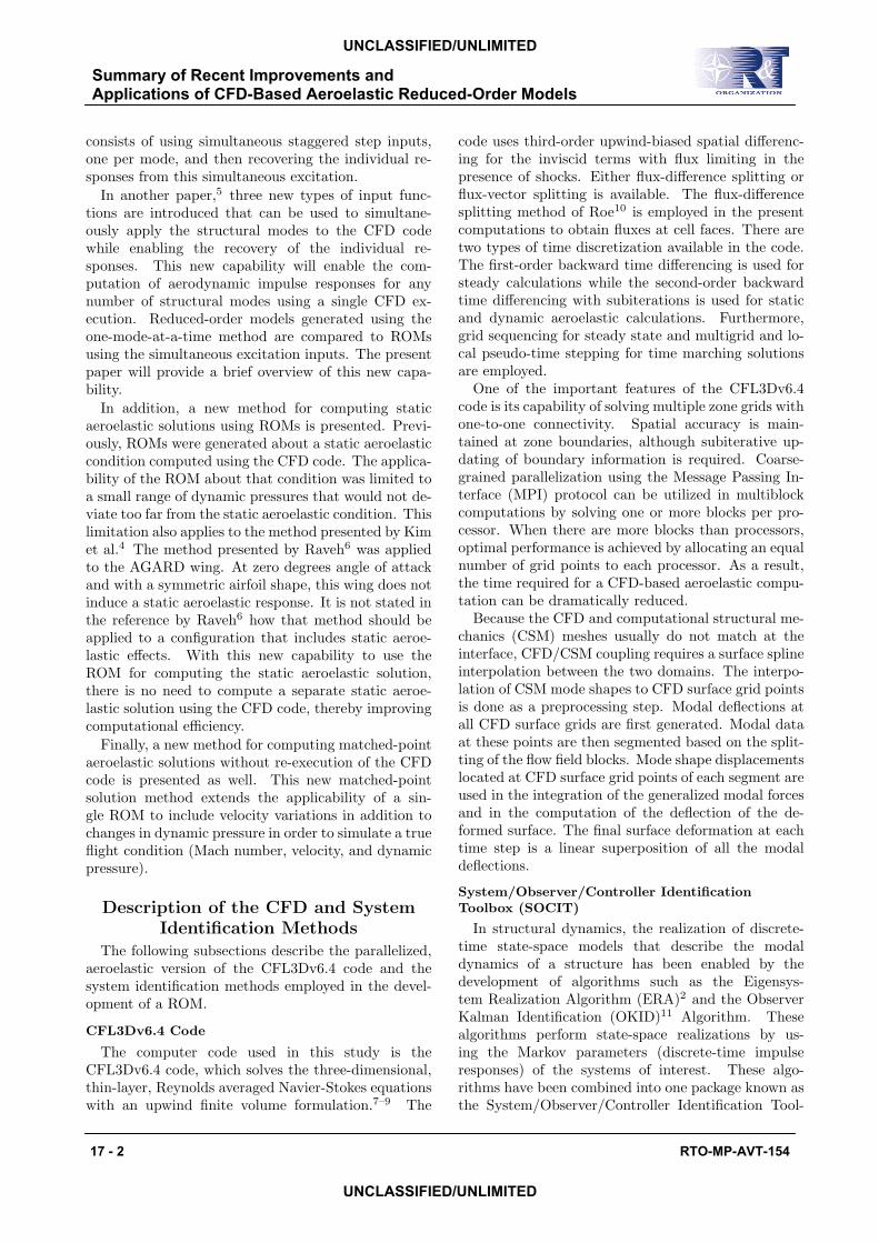
the coupling of a nonlinear unsteady aerodynamic sys-tem (flow solver) with a structural system as depictedin Figure 1. The present study focuses on the devel-opment of a linearized unsteady aerodynamic ROM(in state-space form), using the general procedure de-picted in Figure 2, that is then coupled to a structuralmodel (also in state-space form) for aeroelastic analy-ses. For the discussions that follow, the term ROMwill refer to the unsteady aerodynamic state-spacemodel. When the unsteady aerodynamic state-spacemodel (ROM) is connected to a state-space model ofthe structure within the SIMULINK environment, thissystem is often also referred to as a ROM. However,to avoid confusion, the SIMULINK aeroelastic systemwill be referred to as the aeroelastic simulation ROM.

Fig. 1 Coupling of structure and aerodynamicswithin an aeroelastic CFD code.

An outline of the original (one-mode-at-a-time)ROM development process1 is presented as back-ground for the new enhancements. The original ROMdevelopment process is as follows:

1. Implementation of impulse/step response tech-nique into aeroelastic CFD code;

2. Computation of impulse/step responses for eachmode, one mode at a time, of an aeroelastic systemusing the aeroelastic CFD code; these responses arecomputed about a static aeroelastic solution (or agiven dynamic pressure);

3. Impulse responses generated in Step 2 are trans-formed into an unsteady aerodynamic state-space sys-tem using the ERA (within SOCIT);

4. Evaluation/validation of the state-space modelsgenerated in Step 3 via comparison with CFD results(i.e., ROM results vs. full CFD solution results);


17 - 4 RTO-MP-AVT-154



Fig. 2 Identification of generalized aerodynamicforces (GAFs).

In the original ROM process, since each mode is be-ing excited individually, the response in each outputdue to a particular input (e.g., the impulse responsein output 2 due to input 1) is generated almost di-rectly. If the function being used to excite the systemis an impulse (or a unit pulse for discrete-time sys-tems), then the output from the CFD solution willconsist of the impulse response of each output dueto that one input. If the function being used to ex-cite the system is not an impulse function (such as astep input or a random input), then the impulse re-sponse needs to be extracted from the input/outputdata. One method for extraction is deconvolution1

but there are other methods that can be used. For theoriginal ROM process, since each input to a systemis being excited individually, the exact nature of theinput function is defined, to a certain extent, basedon user preference (frequency range of interest, easeof implementation into a CFD solver, etc.). The stepinput has emerged as a convenient input for the orig-inal ROM process due to its ease of implementationinto a CFD solver and to the wide range of frequencyexcitation that it can generate.

The primary issue,then, with the original ROM pro-cess was the identification of the unsteady aerody-namic impulse responses one mode at a time (Step 2).Clearly, for a large number of modes, this procedurebecomes impractical.

Improved ROM Development ProcessesAn outline of the improved simultaneous modal ex-

citation ROM development process with the recentenhancements is as follows:

1. Generate the number of functions (from a se-

lected family) that corresponds to the number of struc-tural modeshapes;

2. Apply the generated input functions simulta-neously via one CFD execution; these responses arecomputed directly from the restart of a steady rigidCFL3D solution (not about a particular dynamic pres-sure);

3. Using the simultaneous input/output responses,identify the individual impulse responses using thePULSE algorithm (within SOCIT);

4. Transform the individual impulse responses gen-erated in Step 3 into an unsteady aerodynamic state-space system using the ERA(within SOCIT);

5. Evaluate/validate the state-space models gener-ated in Step 4 via comparison with CFD results (i.e.,ROM results vs. full CFD solution results);

An important difference between the original ROMprocess and the improved ROM process is stated insteps (2) of the outlines above. For the original ROMprocess, if a static aeroelastic condition existed, thena ROM was generated about a selected static aeroe-lastic condition. So a static aeroelastic condition ofinterest was defined (typically a dynamic pressure) andthat static aeroelastic condition was computed usingCFL3D as a restart from a converged steady, rigid so-lution. Once a converged static aeroelastic solutionwas obtained, the ROM process was applied aboutthat condition. This implies that the resultant ROMis, of course, limited in some sense to the neighbor-hood of that static aeroelastic condition. Moving ”toofar away” from that condition could result in loss ofaccuracy.

The reason for generating ROMs in this fashionwas because no method had been defined to enablethe computation of a static aeroelastic solution usinga ROM. Any ROMs generated in this fashion were,therefore, limited to the prediction of dynamic re-sponses about a static aeroelastic solution includingthe methods by Raveh6 and by Kim et al.4 The im-proved ROM method, however, includes a method forgenerating a ROM directly from a steady, rigid solu-tion. As a result, these improved ROMs can then beused to predict both static aeroelastic and dynamicsolutions for any dynamic pressure. In order to cap-ture a specific range of aeroelastic effects (previouslyobtained by selecting a particular dynamic pressure),the improved ROM method relies on the excitationamplitude to excite aeroelastic effects of interest. Thedetails of the method for using a ROM for computingboth static aeroelastic and dynamic solutions is pre-sented in another reference by the present author.13

For the present results, all responses were computedfrom the restart of a steady, rigid CFL3D solution,bypassing the need (and additional computational ex-pense) to execute a static aeroelastic solution using


RTO-MP-AVT-154 17 - 5



CFL3D.

Simultaneous Excitation Input Functions

In the situation where the goal is the simulta-neous excitation of a multiple-input multiple-output(MIMO) system, system identification techniques14–16

dictate that the nature of the input functions usedto excite the system must be properly defined if ac-curate input/output models of the system are to begenerated. The most important point to keep in mindwhen defining these input functions is that these func-tions need to be different, in some sense, from eachother. This makes sense since, if the excitation inputsare identical and they are applied simultaneously, itbecomes practically impossible for any system iden-tification algorithm to relate the effects of one inputon a given output. This, in turn, makes it practicallyimpossible for that algorithm to extract the individ-ual impulse responses for each input/output pair. Ashas already been well established, the individual im-pulse responses for each input/output pair are nec-essary ingredients towards the development of state-space models. With respect to unsteady aerodynamicMIMO systems, these individual impulse responsescorrespond to time-domain generalized aerodynamicforces (GAFs), critical to understanding unsteadyaerodynamic behavior. The Fourier-transformed ver-sion of these GAFs are the frequency-domain GAFswhich provide an important link to more traditionalfrequency-domain-based aeroelastic analyses.

The question is how different should these inputfunctions be and how can we quantify a level of ”dif-ference” between each input function? Kim4 uses thefamiliar step function as the input function but witheach step input being applied at a different point intime (lagged) in order to maintain some difference be-tween the input signals. Kim refers to this family oflagged step functions as ”almost orthogonal”. As Kimpoints out, the greater the lag between successive stepinputs, the greater the difference between input sig-nals. This then presents a spectrum of possibilitieswhere, at one end, one has step input functions withno lags (identical functions, not orthogonal) and atthe other end the step functions are separated by anextremely large lag (in the limit, these are the individ-ual step inputs from the original ROM process). Sinceorthogonality (linear independence) is the most pre-cise mathematical method for guaranteeing the ”dif-ference” between signals, the present research focuseson the application of families of orthogonal functionsas candidate input functions. Using orthogonal func-tions directly provides a mathematical guarantee thatthe input functions are as different as mathematicallypossible. These orthogonal input functions then canbe considered optimal input functions for the identifi-

cation of a MIMO system.In the paper by Silva,5 four families of functions

were applied towards the efficient identification of aCFD-based unsteady aerodynamic state-space model:lagged step, block pulse, Haar, and Walsh. Althoughit has been stated by Kim that the lagged-step func-tions are not completely orthogonal (almost orthogo-nal), these functions are used in the present study forcomparison purposes. The other three functions eachrepresent an orthogonal family of functions. The blockpulse functions, presented in Figure 3, are orthogonaland resemble a modified step input. An advantage ofstep-like functions is the broad frequency bandwidththat is excited by the impulsive nature of these func-tions. An added benefit of the block pulse functionsover traditional step functions is that block pulse in-puts provide excitation to the system in both positiveand negative directions. From an unsteady aerody-namics point of view, it is important that modes of re-alistic wing configurations (e.g., with a non-symmetricairfoil) be excited in both directions for a more com-plete capture of relevant dynamics. For the presentpaper, results will be limited to the application ofWalsh functions with a limited overview of the otherfunctions.

Fig. 3 Block pulse functions.

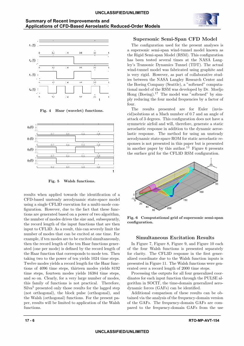
The Haar functions, presented in Figure 4, com-prise one of the simplest form of wavelet functions.These functions are orthogonal by the mathematicaldefinition of wavelet functions. Likewise, this familyof functions has a similarity to step inputs and there-fore embodies the impulsive (i.e., beneficial) nature ofstep inputs with regards to frequency bandwidth. Thefinal set of orthogonal functions is the Walsh function,presented in Figure 5.

It is important to mention that the Haar functionsare generated using formulas based on a power oftwo algorithm. These functions have yielded excellent


17 - 6 RTO-MP-AVT-154



Fig. 4 Haar (wavelet) functions.

Fig. 5 Walsh functions.

results when applied towards the identification of aCFD-based unsteady aerodynamic state-space modelusing a single CFL3D execution for a multi-mode con-figuration. However, due to the fact that these func-tions are generated based on a power of two algorithm,the number of modes drives the size and, subsequently,the record length of the input functions that are theninput to CFL3D. As a result, this can severely limit thenumber of modes that can be excited at one time. Forexample, if ten modes are to be excited simultaneously,then the record length of the ten Haar functions gener-ated (one per mode) is defined by the record length ofthe Haar function that corresponds to mode ten. Thentaking two to the power of ten yields 1024 time steps.Twelve modes yields a record length for the Haar func-tions of 4096 time steps, thirteen modes yields 8192time steps, fourteen modes yields 16384 time steps,and so on. Clearly, for a very large number of modes,this family of functions is not practical. Therefore,Silva5 presented only those results for the lagged step(not orthogonal), the block pulse (orthogonal), andthe Walsh (orthogonal) functions. For the present pa-per, results will be limited to application of the Walshfunctions.

Supersonic Semi-Span CFD ModelThe configuration used for the present analyses is

a supersonic semi-span wind-tunnel model known asthe Rigid Semi-span Model (RSM). This configurationhas been tested several times at the NASA Lang-ley’s Transonic Dynamics Tunnel (TDT). The actualwind-tunnel model was fabricated using graphite andis very rigid. However, as part of collaborative stud-ies between the NASA Langley Research Center andthe Boeing Company (Seattle), a ”softened” computa-tional model of the RSM was developed by Dr. MoeljoHong (Boeing).17 The model was ”softened” by sim-ply reducing the four modal frequencies by a factor offour.

The results presented are for Euler (invis-cid)solutions at a Mach number of 0.7 and an angle ofattack of 3 degrees. This configuration does not have asymmetric airfoil and will, therefore, generate a staticaeroelastic response in addition to the dynamic aeroe-lastic response. The method for using an unsteadyaerodynamic state-space ROM for static aeroelastic re-sponses is not presented in this paper but is presentedin another paper by this author.13 Figure 6 presentsthe surface grid for the CFL3D RSM configuration.

Fig. 6 Computational grid of supersonic semi-spanconfiguration.

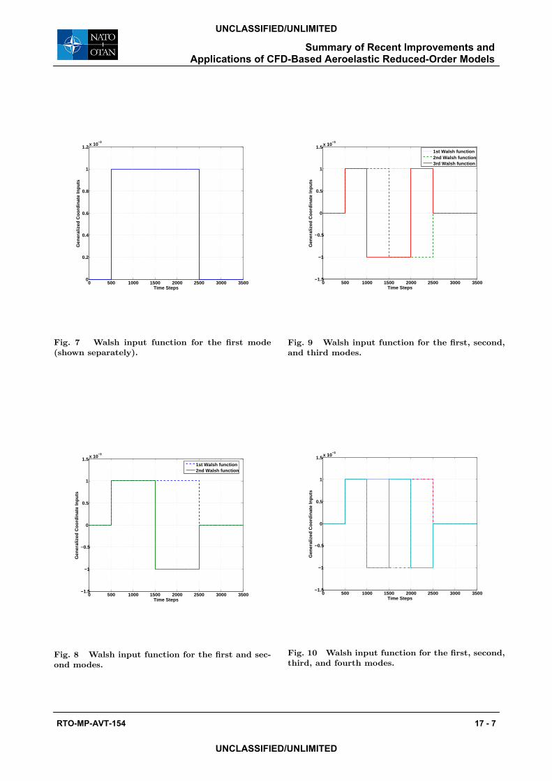
Simultaneous Excitation ResultsIn Figure 7, Figure 8, Figure 9, and Figure 10 each

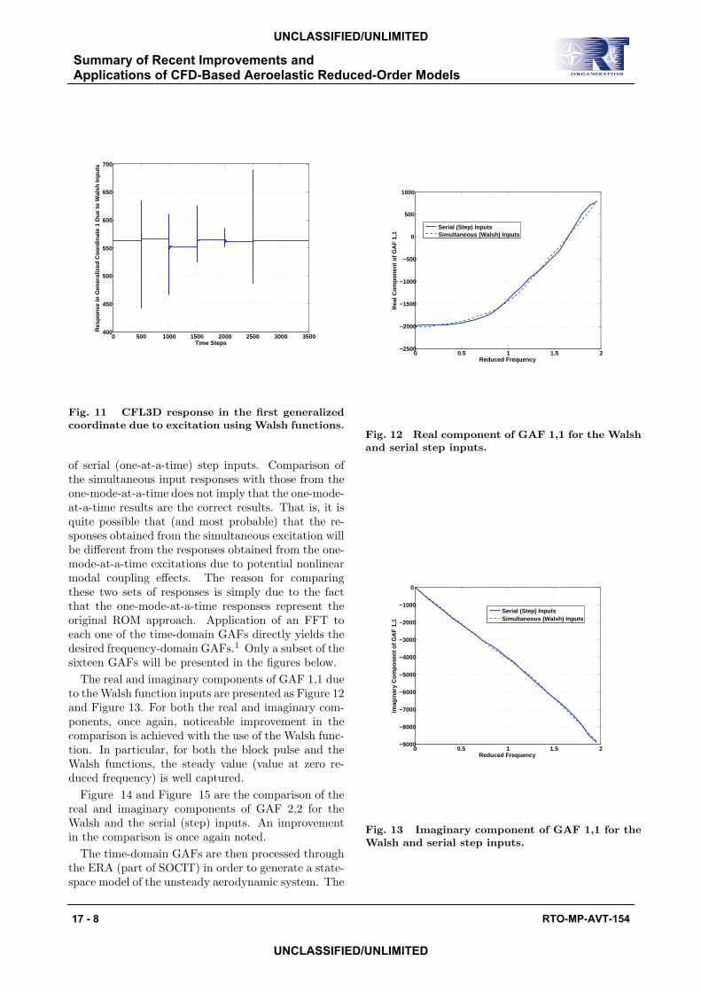
of the four Walsh functions is presented separatelyfor clarity. The CFL3D response in the first gener-alized coordinate due to the Walsh function inputs ispresented in Figure 11. The Walsh functions were gen-erated over a record length of 2000 time steps.

Processing the outputs for all four generalized coor-dinates for each input function through the PULSE al-gorithm in SOCIT, the time-domain generalized aero-dynamic forces (GAFs) can be identified.

Additional comparison of these results can be ob-tained via the analysis of the frequency-domain versionof the GAFs. The frequency-domain GAFs are com-pared to the frequency-domain GAFs from the use


RTO-MP-AVT-154 17 - 7



0 500 1000 1500 2000 2500 3000 35000

0.2

0.4

0.6

0.8

1

1.2x 10

−3

Time Steps

Gen

eral

ized

Coo

rdin

ate

Inpu

ts

Fig. 7 Walsh input function for the first mode(shown separately).

0 500 1000 1500 2000 2500 3000 3500−1.5

−1

−0.5

0

0.5

1

1.5x 10

−3

Time Steps

Gen

eral

ized

Coo

rdin

ate

Inpu

ts

1st Walsh function2nd Walsh function

Fig. 8 Walsh input function for the first and sec-ond modes.

0 500 1000 1500 2000 2500 3000 3500−1.5

−1

−0.5

0

0.5

1

1.5x 10

−3

Time Steps

Gen

eral

ized

Coo

rdin

ate

Inpu

ts

1st Walsh function2nd Walsh function3rd Walsh function

Fig. 9 Walsh input function for the first, second,and third modes.

0 500 1000 1500 2000 2500 3000 3500−1.5

−1

−0.5

0

0.5

1

1.5x 10

−3

Time Steps

Gen

eral

ized

Coo

rdin

ate

Inpu

ts

Fig. 10 Walsh input function for the first, second,third, and fourth modes.


17 - 8 RTO-MP-AVT-154



0 500 1000 1500 2000 2500 3000 3500400

450

500

550

600

650

700

Time Steps

Res

po

nse

in G

ener

aliz

ed C

oo

rdin

ate

1 D

ue

to W

alsh

Inp

uts

Fig. 11 CFL3D response in the first generalizedcoordinate due to excitation using Walsh functions.

of serial (one-at-a-time) step inputs. Comparison ofthe simultaneous input responses with those from theone-mode-at-a-time does not imply that the one-mode-at-a-time results are the correct results. That is, it isquite possible that (and most probable) that the re-sponses obtained from the simultaneous excitation willbe different from the responses obtained from the one-mode-at-a-time excitations due to potential nonlinearmodal coupling effects. The reason for comparingthese two sets of responses is simply due to the factthat the one-mode-at-a-time responses represent theoriginal ROM approach. Application of an FFT toeach one of the time-domain GAFs directly yields thedesired frequency-domain GAFs.1 Only a subset of thesixteen GAFs will be presented in the figures below.

The real and imaginary components of GAF 1,1 dueto the Walsh function inputs are presented as Figure 12and Figure 13. For both the real and imaginary com-ponents, once again, noticeable improvement in thecomparison is achieved with the use of the Walsh func-tion. In particular, for both the block pulse and theWalsh functions, the steady value (value at zero re-duced frequency) is well captured.

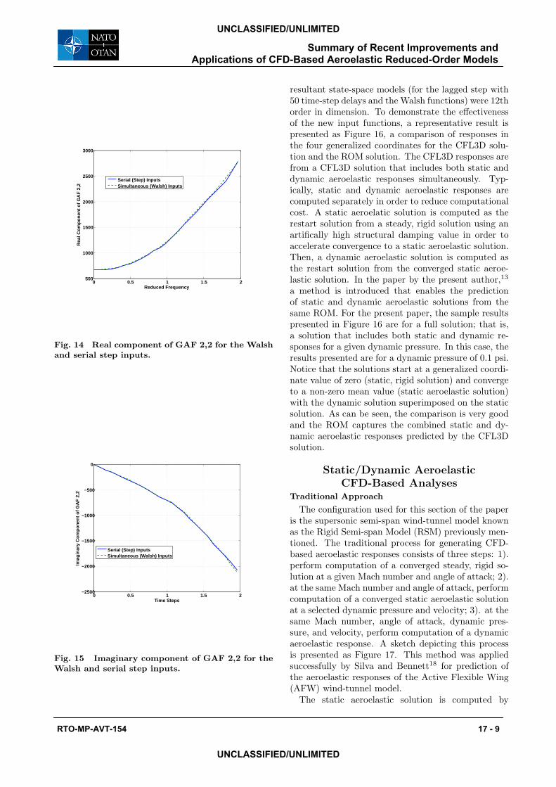
Figure 14 and Figure 15 are the comparison of thereal and imaginary components of GAF 2,2 for theWalsh and the serial (step) inputs. An improvementin the comparison is once again noted.

The time-domain GAFs are then processed throughthe ERA (part of SOCIT) in order to generate a state-space model of the unsteady aerodynamic system. The

0 0.5 1 1.5 2−2500

−2000

−1500

−1000

−500

0

500

1000

Reduced Frequency

Rea

l Com

pone

nt o

f GA

F 1

,1

Serial (Step) InputsSimultaneous (Walsh) Inputs

Fig. 12 Real component of GAF 1,1 for the Walshand serial step inputs.

0 0.5 1 1.5 2−9000

−8000

−7000

−6000

−5000

−4000

−3000

−2000

−1000

0

Reduced Frequency

Imag

inar

y C

ompo

nent

of G

AF

1,1


Fig. 13 Imaginary component of GAF 1,1 for theWalsh and serial step inputs.


RTO-MP-AVT-154 17 - 9



0 0.5 1 1.5 2500

1000

1500

2000

2500

3000

Reduced Frequency

Rea

l Co

mp

on

ent

of

GA

F 2

,2


Fig. 14 Real component of GAF 2,2 for the Walshand serial step inputs.

0 0.5 1 1.5 2−2500

−2000

−1500

−1000

−500

0

Time Steps

Imag

inar

y C

ompo

nent

of G

AF

2,2


Fig. 15 Imaginary component of GAF 2,2 for theWalsh and serial step inputs.

resultant state-space models (for the lagged step with50 time-step delays and the Walsh functions) were 12thorder in dimension. To demonstrate the effectivenessof the new input functions, a representative result ispresented as Figure 16, a comparison of responses inthe four generalized coordinates for the CFL3D solu-tion and the ROM solution. The CFL3D responses arefrom a CFL3D solution that includes both static anddynamic aeroelastic responses simultaneously. Typ-ically, static and dynamic aeroelastic responses arecomputed separately in order to reduce computationalcost. A static aeroelatic solution is computed as therestart solution from a steady, rigid solution using anartifically high structural damping value in order toaccelerate convergence to a static aeroelastic solution.Then, a dynamic aeroelastic solution is computed asthe restart solution from the converged static aeroe-lastic solution. In the paper by the present author,13

a method is introduced that enables the predictionof static and dynamic aeroelastic solutions from thesame ROM. For the present paper, the sample resultspresented in Figure 16 are for a full solution; that is,a solution that includes both static and dynamic re-sponses for a given dynamic pressure. In this case, theresults presented are for a dynamic pressure of 0.1 psi.Notice that the solutions start at a generalized coordi-nate value of zero (static, rigid solution) and convergeto a non-zero mean value (static aeroelastic solution)with the dynamic solution superimposed on the staticsolution. As can be seen, the comparison is very goodand the ROM captures the combined static and dy-namic aeroelastic responses predicted by the CFL3Dsolution.

Static/Dynamic AeroelasticCFD-Based Analyses

Traditional Approach

The configuration used for this section of the paperis the supersonic semi-span wind-tunnel model knownas the Rigid Semi-span Model (RSM) previously men-tioned. The traditional process for generating CFD-based aeroelastic responses consists of three steps: 1).perform computation of a converged steady, rigid so-lution at a given Mach number and angle of attack; 2).at the same Mach number and angle of attack, performcomputation of a converged static aeroelastic solutionat a selected dynamic pressure and velocity; 3). at thesame Mach number, angle of attack, dynamic pres-sure, and velocity, perform computation of a dynamicaeroelastic response. A sketch depicting this processis presented as Figure 17. This method was appliedsuccessfully by Silva and Bennett18 for prediction ofthe aeroelastic responses of the Active Flexible Wing(AFW) wind-tunnel model.

The static aeroelastic solution is computed by


17 - 10 RTO-MP-AVT-154



0 500 1000 1500 20000

0.05

0.1

Gen

Coo

rd 1

0 200 400 600 800 1000 1200 1400 1600−0.04

−0.02

0

Gen

Coo

rd 2

0 500 1000 1500 2000−5

0

5x 10

−3

Gen

Coo

rd 3

0 500 1000 1500 2000−1

0

1x 10

−3

Time Steps

Gen

Coo

rd 4

ROM (Walsh)CFL3D

Fig. 16 Full solution (static plus dynamic aeroe-lastic responses) generalized coordinate responsesat a dynamic pressure of 0.1 psi.

Fig. 17 Sketch depicting the traditional processfor generating CFD-based aeroelastic responses.

restarting the converged steady, rigid solution. Theconverged steady, rigid solution, therefore serves asthe initial condition for the static aeroelastic solu-tion. Likewise, the converged static aeroelastic solu-tion serves as the initial condition for the dynamicaeroelastic solution. The static aeroelastic solutionis computed by imposing a very large value of modaldamping to the system, thereby attenuating dynamictransients and yielding static aeroelastic deflections.In addition, the initial conditions (initial generalizeddisplacements and velocities) are set to zero withinthe structural integrator portion of CFL3D. An ex-

ample of a static aeroelastic solution for the softenedRSM configuration is presented as Figure 18 wherethe artificially-excessive modal damping (0.99) resultsin an acceleration of the static aeroelastic convergenceby attenuating dynamic transients.

Fig. 18 Converged static aeroelastic solution forthe RSM configuration at 0.7 Mach number, 3 de-grees angle of attack, and 0.1 psi dynamic pressure.

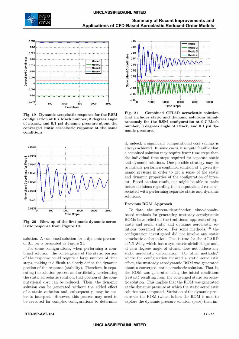
Upon achieving a converged static aeroelastic so-lution, a dynamic solution is computed by restartingthe static aeroelastic solution. The restarting of a so-lution file basically defines the initial structural andflow conditions from the previous solution (the staticaeroelastic solution in this case). For the dynamic so-lution, the value of modal damping is set to a realisticvalue (typically zero or on the order of 1-3 percent ofcritical). The initial conditions of the structure arenow set to non-zero values in order to provide an ini-tial excitation to the system. Typically, generalizedvelocities are set to some small value while the gen-eralized displacements are set to zero. The resultantdynamic aeroelastic solution for zero modal dampingand a value of 0.001 for all four generalized velocities ispresented as Figure 19. Zooming in on the first gener-alized coordinate, presented as Figure 20, the stabilityof the dynamic response can be ascertained. How-ever, post-processing of the generalized aerodynamictransients is required to obtain damping and frequencyestimates.

The primary reason for performing separate and se-rial static and dynamic aeroelastic solutions18 was forcomputational efficiency, as follows. Clearly, a solutioncan be obtained which contains both the static anddynamic solutions occurring simultaneously by settingmodal damping to zero (or a small value), setting thestructural initial conditions (generalized velocities) tosmall non-zero values, and restarting this combined so-lution from the restart file of a converged steady, rigid


RTO-MP-AVT-154 17 - 11



Fig. 19 Dynamic aeroelastic response for the RSMconfiguration at 0.7 Mach number, 3 degrees angleof attack, and 0.1 psi dynamic pressure about theconverged static aeroelastic response at the sameconditions.

Fig. 20 Blow up of the first mode dynamic aeroe-lastic response from Figure 19.

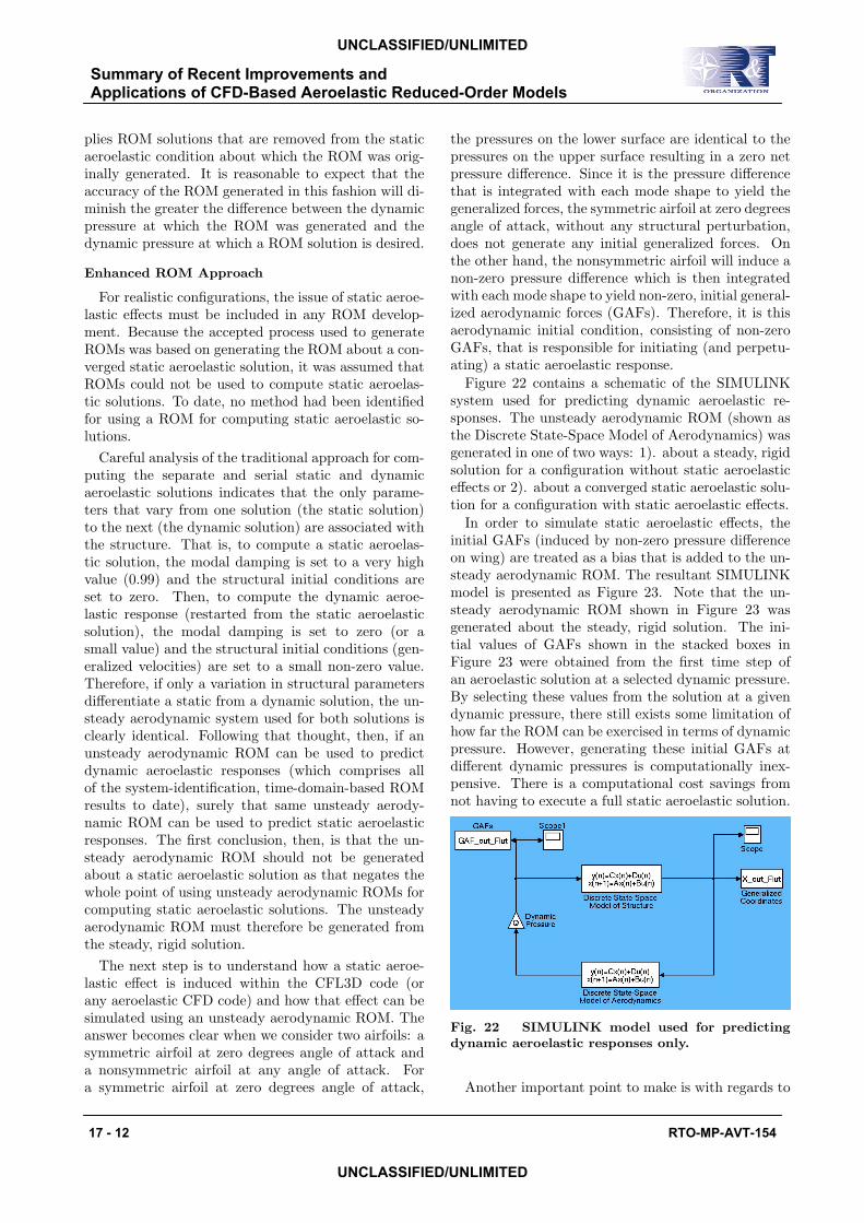
solution. A combined solution for a dynamic pressureof 0.1 psi is presented as Figure 21.

For some configurations, when performing a com-bined solution, the convergence of the static portionof the response could require a large number of timesteps, making it difficult to clearly define the dynamicportion of the response (stability). Therefore, in sepa-rating the solution process and artificially acceleratingthe static aeroelastic solution, that portion of the com-putational cost can be reduced. Then, the dynamicsolution can be generated without the added effectof a static variation and, subsequently, may be eas-ier to interpret. However, this process may need tobe revisited for complex configurations to determine

Fig. 21 Combined CFL3D aeroelastic solutionthat includes static and dynamic solutions simul-taneously for the RSM configuration at 0.7 Machnumber, 3 degrees angle of attack, and 0.1 psi dy-namic pressure.

if, indeed, a significant computational cost savings isalways achieved. In some cases, it is quite feasible thata combined solution may require fewer time steps thanthe individual time steps required for separate staticand dynamic solutions. One possible strategy may beto initially perform a combined solution at a given dy-namic pressure in order to get a sense of the staticand dynamic properties of the configuration of inter-est. Based on that result, one might be able to makebetter decisions regarding the computational costs as-sociated with performing separate static and dynamicsolutions.

Previous ROM Approach

To date, the system-identification, time-domain-based methods for generating unsteady aerodynamicROMs have relied on the traditional approach of sep-arate and serial static and dynamic aeroelastic so-lutions presented above. For some methods,1,6 theconfiguration investigated did not involve any staticaeroelastic deformation. This is true for the AGARD445.6 Wing which has a symmetric airfoil shape and,at zero degrees angle of attack, does not induce anystatic aeroelastic deformation. For other methods,4

where the configuration induced a static aeroelasticeffect, the unsteady aerodynamic ROM was generatedabout a converged static aeroelastic solution. That is,the ROM was generated using the initial conditions(restart) resulting from the converged static aeroelas-tic solution. This implies that the ROM was generatedat the dynamic pressure at which the static aeroelasticsolution was computed. Variation of the dynamic pres-sure via the ROM (which is how the ROM is used toexplore the dynamic pressure solution space) then im-


17 - 12 RTO-MP-AVT-154



plies ROM solutions that are removed from the staticaeroelastic condition about which the ROM was orig-inally generated. It is reasonable to expect that theaccuracy of the ROM generated in this fashion will di-minish the greater the difference between the dynamicpressure at which the ROM was generated and thedynamic pressure at which a ROM solution is desired.

Enhanced ROM Approach

For realistic configurations, the issue of static aeroe-lastic effects must be included in any ROM develop-ment. Because the accepted process used to generateROMs was based on generating the ROM about a con-verged static aeroelastic solution, it was assumed thatROMs could not be used to compute static aeroelas-tic solutions. To date, no method had been identifiedfor using a ROM for computing static aeroelastic so-lutions.

Careful analysis of the traditional approach for com-puting the separate and serial static and dynamicaeroelastic solutions indicates that the only parame-ters that vary from one solution (the static solution)to the next (the dynamic solution) are associated withthe structure. That is, to compute a static aeroelas-tic solution, the modal damping is set to a very highvalue (0.99) and the structural initial conditions areset to zero. Then, to compute the dynamic aeroe-lastic response (restarted from the static aeroelasticsolution), the modal damping is set to zero (or asmall value) and the structural initial conditions (gen-eralized velocities) are set to a small non-zero value.Therefore, if only a variation in structural parametersdifferentiate a static from a dynamic solution, the un-steady aerodynamic system used for both solutions isclearly identical. Following that thought, then, if anunsteady aerodynamic ROM can be used to predictdynamic aeroelastic responses (which comprises allof the system-identification, time-domain-based ROMresults to date), surely that same unsteady aerody-namic ROM can be used to predict static aeroelasticresponses. The first conclusion, then, is that the un-steady aerodynamic ROM should not be generatedabout a static aeroelastic solution as that negates thewhole point of using unsteady aerodynamic ROMs forcomputing static aeroelastic solutions. The unsteadyaerodynamic ROM must therefore be generated fromthe steady, rigid solution.

The next step is to understand how a static aeroe-lastic effect is induced within the CFL3D code (orany aeroelastic CFD code) and how that effect can besimulated using an unsteady aerodynamic ROM. Theanswer becomes clear when we consider two airfoils: asymmetric airfoil at zero degrees angle of attack anda nonsymmetric airfoil at any angle of attack. Fora symmetric airfoil at zero degrees angle of attack,

the pressures on the lower surface are identical to thepressures on the upper surface resulting in a zero netpressure difference. Since it is the pressure differencethat is integrated with each mode shape to yield thegeneralized forces, the symmetric airfoil at zero degreesangle of attack, without any structural perturbation,does not generate any initial generalized forces. Onthe other hand, the nonsymmetric airfoil will induce anon-zero pressure difference which is then integratedwith each mode shape to yield non-zero, initial general-ized aerodynamic forces (GAFs). Therefore, it is thisaerodynamic initial condition, consisting of non-zeroGAFs, that is responsible for initiating (and perpetu-ating) a static aeroelastic response.

Figure 22 contains a schematic of the SIMULINKsystem used for predicting dynamic aeroelastic re-sponses. The unsteady aerodynamic ROM (shown asthe Discrete State-Space Model of Aerodynamics) wasgenerated in one of two ways: 1). about a steady, rigidsolution for a configuration without static aeroelasticeffects or 2). about a converged static aeroelastic solu-tion for a configuration with static aeroelastic effects.

In order to simulate static aeroelastic effects, theinitial GAFs (induced by non-zero pressure differenceon wing) are treated as a bias that is added to the un-steady aerodynamic ROM. The resultant SIMULINKmodel is presented as Figure 23. Note that the un-steady aerodynamic ROM shown in Figure 23 wasgenerated about the steady, rigid solution. The ini-tial values of GAFs shown in the stacked boxes inFigure 23 were obtained from the first time step ofan aeroelastic solution at a selected dynamic pressure.By selecting these values from the solution at a givendynamic pressure, there still exists some limitation ofhow far the ROM can be exercised in terms of dynamicpressure. However, generating these initial GAFs atdifferent dynamic pressures is computationally inex-pensive. There is a computational cost savings fromnot having to execute a full static aeroelastic solution.

Fig. 22 SIMULINK model used for predictingdynamic aeroelastic responses only.

Another important point to make is with regards to


RTO-MP-AVT-154 17 - 13



the level of excitation used to generate an unsteadyaerodynamic ROM. In the previous method, where aROM is generated about a converged static aeroelas-tic solution (i.e., a particular dynamic pressure), theselection of the dynamic pressure defines a region ofaeroelastic behavior that is of interest. For exam-ple, if it is expected that the unsteady flow field willvary significantly beyond some elastic deformation ofthe structure, that elastic deformation corresponds tosome value of dynamic pressure. The desired ROMcan then be generated about that condition in orderto capture important unsteady aerodynamic effects.With the new method for generating ROMs, sincethe unsteady aerodynamic ROM is generated from asteady, rigid solution, it is independent of dynamicpressure. With the new method, instead of using dy-namic pressure to excite a particular range of unsteadyaerodynamic behavior, it is the magnitude of the gen-eralized coordinates (used as input to the unsteadyaerodynamic system to define the ROM) that definesa particular region of interest.

Fig. 23 SIMULINK model used for predictingboth or either static and dynamic aeroelastic re-sponses.

Comparison of various CFL3D and ROM static, dy-namic, and combined aeroelastic responses are nowpresented. In another paper,5 three new orthogonalfunctions are introduced that can be used to simulta-neously excite all the modes of an unsteady aerody-namic system in order to generate an unsteady aero-dynamic ROM with a single CFD execution. For theresults that follow, the unsteady aerodynamic ROMwas generated using the Walsh functions.5

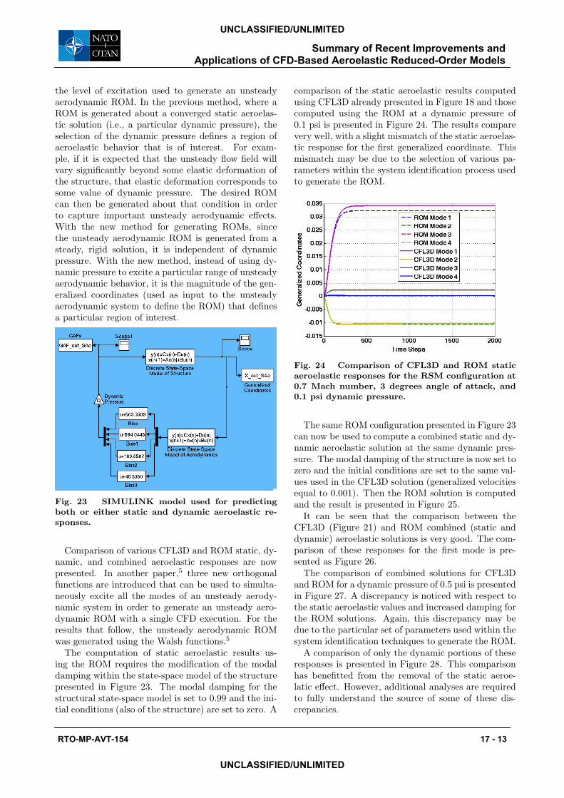
The computation of static aeroelastic results us-ing the ROM requires the modification of the modaldamping within the state-space model of the structurepresented in Figure 23. The modal damping for thestructural state-space model is set to 0.99 and the ini-tial conditions (also of the structure) are set to zero. A

comparison of the static aeroelastic results computedusing CFL3D already presented in Figure 18 and thosecomputed using the ROM at a dynamic pressure of0.1 psi is presented in Figure 24. The results comparevery well, with a slight mismatch of the static aeroelas-tic response for the first generalized coordinate. Thismismatch may be due to the selection of various pa-rameters within the system identification process usedto generate the ROM.

Fig. 24 Comparison of CFL3D and ROM staticaeroelastic responses for the RSM configuration at0.7 Mach number, 3 degrees angle of attack, and0.1 psi dynamic pressure.

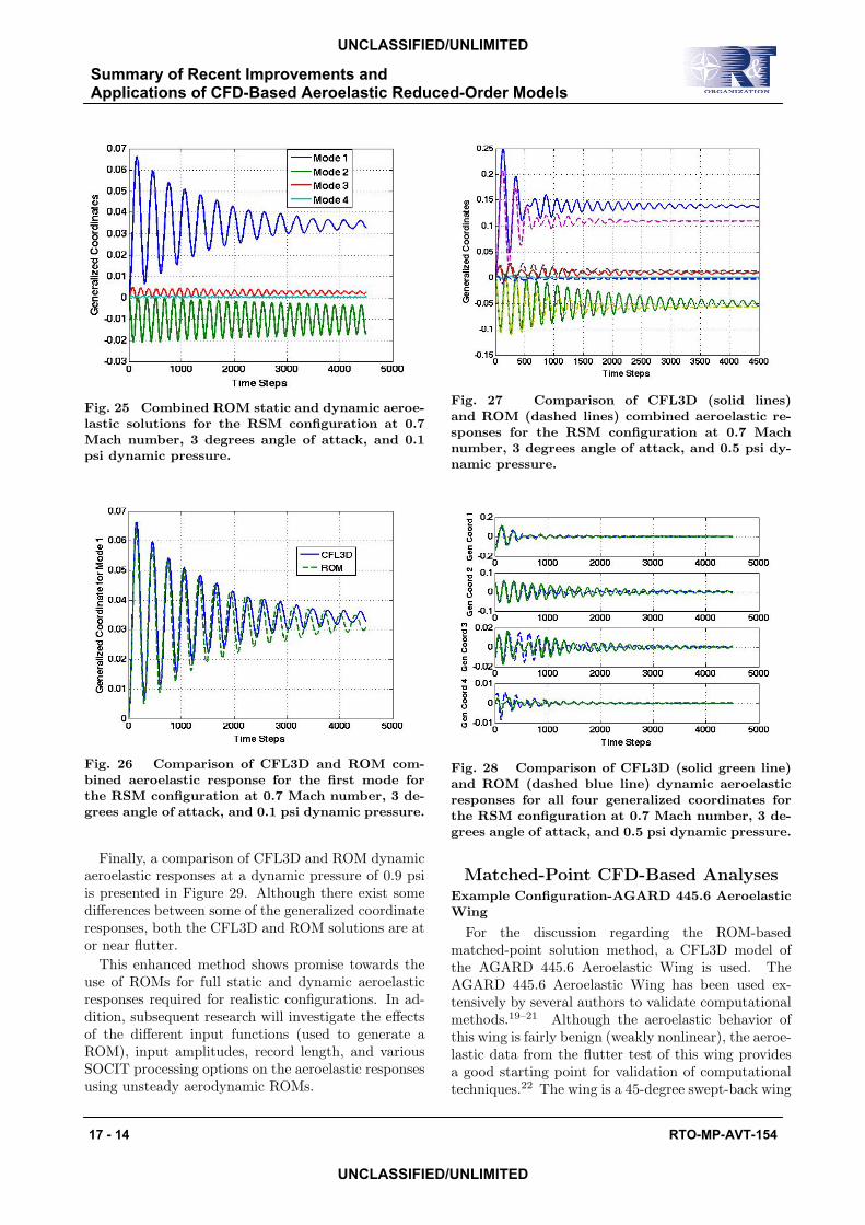
The same ROM configuration presented in Figure 23can now be used to compute a combined static and dy-namic aeroelastic solution at the same dynamic pres-sure. The modal damping of the structure is now set tozero and the initial conditions are set to the same val-ues used in the CFL3D solution (generalized velocitiesequal to 0.001). Then the ROM solution is computedand the result is presented in Figure 25.

It can be seen that the comparison between theCFL3D (Figure 21) and ROM combined (static anddynamic) aeroelastic solutions is very good. The com-parison of these responses for the first mode is pre-sented as Figure 26.

The comparison of combined solutions for CFL3Dand ROM for a dynamic pressure of 0.5 psi is presentedin Figure 27. A discrepancy is noticed with respect tothe static aeroelastic values and increased damping forthe ROM solutions. Again, this discrepancy may bedue to the particular set of parameters used within thesystem identification techniques to generate the ROM.

A comparison of only the dynamic portions of theseresponses is presented in Figure 28. This comparisonhas benefitted from the removal of the static aeroe-latic effect. However, additional analyses are requiredto fully understand the source of some of these dis-crepancies.


17 - 14 RTO-MP-AVT-154



Fig. 25 Combined ROM static and dynamic aeroe-lastic solutions for the RSM configuration at 0.7Mach number, 3 degrees angle of attack, and 0.1psi dynamic pressure.

Fig. 26 Comparison of CFL3D and ROM com-bined aeroelastic response for the first mode forthe RSM configuration at 0.7 Mach number, 3 de-grees angle of attack, and 0.1 psi dynamic pressure.

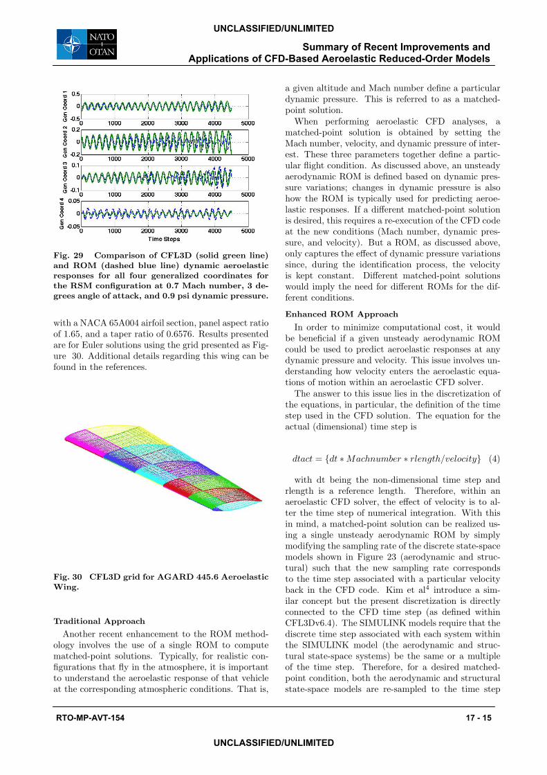
Finally, a comparison of CFL3D and ROM dynamicaeroelastic responses at a dynamic pressure of 0.9 psiis presented in Figure 29. Although there exist somedifferences between some of the generalized coordinateresponses, both the CFL3D and ROM solutions are ator near flutter.

This enhanced method shows promise towards theuse of ROMs for full static and dynamic aeroelasticresponses required for realistic configurations. In ad-dition, subsequent research will investigate the effectsof the different input functions (used to generate aROM), input amplitudes, record length, and variousSOCIT processing options on the aeroelastic responsesusing unsteady aerodynamic ROMs.

Fig. 27 Comparison of CFL3D (solid lines)and ROM (dashed lines) combined aeroelastic re-sponses for the RSM configuration at 0.7 Machnumber, 3 degrees angle of attack, and 0.5 psi dy-namic pressure.

Fig. 28 Comparison of CFL3D (solid green line)and ROM (dashed blue line) dynamic aeroelasticresponses for all four generalized coordinates forthe RSM configuration at 0.7 Mach number, 3 de-grees angle of attack, and 0.5 psi dynamic pressure.

Matched-Point CFD-Based AnalysesExample Configuration-AGARD 445.6 AeroelasticWing

For the discussion regarding the ROM-basedmatched-point solution method, a CFL3D model ofthe AGARD 445.6 Aeroelastic Wing is used. TheAGARD 445.6 Aeroelastic Wing has been used ex-tensively by several authors to validate computationalmethods.19–21 Although the aeroelastic behavior ofthis wing is fairly benign (weakly nonlinear), the aeroe-lastic data from the flutter test of this wing providesa good starting point for validation of computationaltechniques.22 The wing is a 45-degree swept-back wing


RTO-MP-AVT-154 17 - 15



Fig. 29 Comparison of CFL3D (solid green line)and ROM (dashed blue line) dynamic aeroelasticresponses for all four generalized coordinates forthe RSM configuration at 0.7 Mach number, 3 de-grees angle of attack, and 0.9 psi dynamic pressure.

with a NACA 65A004 airfoil section, panel aspect ratioof 1.65, and a taper ratio of 0.6576. Results presentedare for Euler solutions using the grid presented as Fig-ure 30. Additional details regarding this wing can befound in the references.

Fig. 30 CFL3D grid for AGARD 445.6 AeroelasticWing.

Traditional Approach

Another recent enhancement to the ROM method-ology involves the use of a single ROM to computematched-point solutions. Typically, for realistic con-figurations that fly in the atmosphere, it is importantto understand the aeroelastic response of that vehicleat the corresponding atmospheric conditions. That is,

a given altitude and Mach number define a particulardynamic pressure. This is referred to as a matched-point solution.

When performing aeroelastic CFD analyses, amatched-point solution is obtained by setting theMach number, velocity, and dynamic pressure of inter-est. These three parameters together define a partic-ular flight condition. As discussed above, an unsteadyaerodynamic ROM is defined based on dynamic pres-sure variations; changes in dynamic pressure is alsohow the ROM is typically used for predicting aeroe-lastic responses. If a different matched-point solutionis desired, this requires a re-execution of the CFD codeat the new conditions (Mach number, dynamic pres-sure, and velocity). But a ROM, as discussed above,only captures the effect of dynamic pressure variationssince, during the identification process, the velocityis kept constant. Different matched-point solutionswould imply the need for different ROMs for the dif-ferent conditions.

Enhanced ROM Approach

In order to minimize computational cost, it wouldbe beneficial if a given unsteady aerodynamic ROMcould be used to predict aeroelastic responses at anydynamic pressure and velocity. This issue involves un-derstanding how velocity enters the aeroelastic equa-tions of motion within an aeroelastic CFD solver.

The answer to this issue lies in the discretization ofthe equations, in particular, the definition of the timestep used in the CFD solution. The equation for theactual (dimensional) time step is

dtact = {dt ∗ Machnumber ∗ rlength/velocity} (4)

with dt being the non-dimensional time step andrlength is a reference length. Therefore, within anaeroelastic CFD solver, the effect of velocity is to al-ter the time step of numerical integration. With thisin mind, a matched-point solution can be realized us-ing a single unsteady aerodynamic ROM by simplymodifying the sampling rate of the discrete state-spacemodels shown in Figure 23 (aerodynamic and struc-tural) such that the new sampling rate correspondsto the time step associated with a particular velocityback in the CFD code. Kim et al4 introduce a sim-ilar concept but the present discretization is directlyconnected to the CFD time step (as defined withinCFL3Dv6.4). The SIMULINK models require that thediscrete time step associated with each system withinthe SIMULINK model (the aerodynamic and struc-tural state-space systems) be the same or a multipleof the time step. Therefore, for a desired matched-point condition, both the aerodynamic and structuralstate-space models are re-sampled to the time step


17 - 16 RTO-MP-AVT-154



consistent with the CFL3D time step. This is a verysimple concept and the results are presented below.

Figure 31 presents a comparison of the generalizedcoordinate responses generated using a single unsteadyaerodynamic ROM of the AGARD 445.6 Wing1 ata dynamic pressure of 75 psf and a velocity of 973ft/sec and the corresponding generalized coordinateresponses from the direct CFL3D solution, both atM=0.9. These results were computed using the one-mode-at-a-time approach. Clearly, since the ROMused for this analysis was generated at this velocity,the comparison is excellent.

As stated above, the goal of the ROM matched-point solution technique is to be able to use a singleunsteady aerodynamic ROM to predict the responseof the aeroelastic system at various combinations ofdynamic pressure and velocity in order to generatematched-point solutions. Defining a new time stepbased on a different velocity, a modified unsteady aero-dynamic ROM and structural state-space model aregenerated using re-sampling techniques available inMATLAB. This is done by basically resampling thediscrete-time systems at the new time step. Figure 32presents a comparison of the generalized coordinateresponses generated using a re-sampled version of theunsteady aerodynamic ROM at a dynamic pressure of70 psf and a velocity of 400 ft/sec and the correspond-ing generalized coordinate responses from the directCFL3D solution. As can be seen, the matched-pointtechnique enables the use of a single unsteady aerody-namic ROM (although re-sampled to match velocity)to compute the response of the aeroelastic system toa variation in dynamic pressure and velocity.

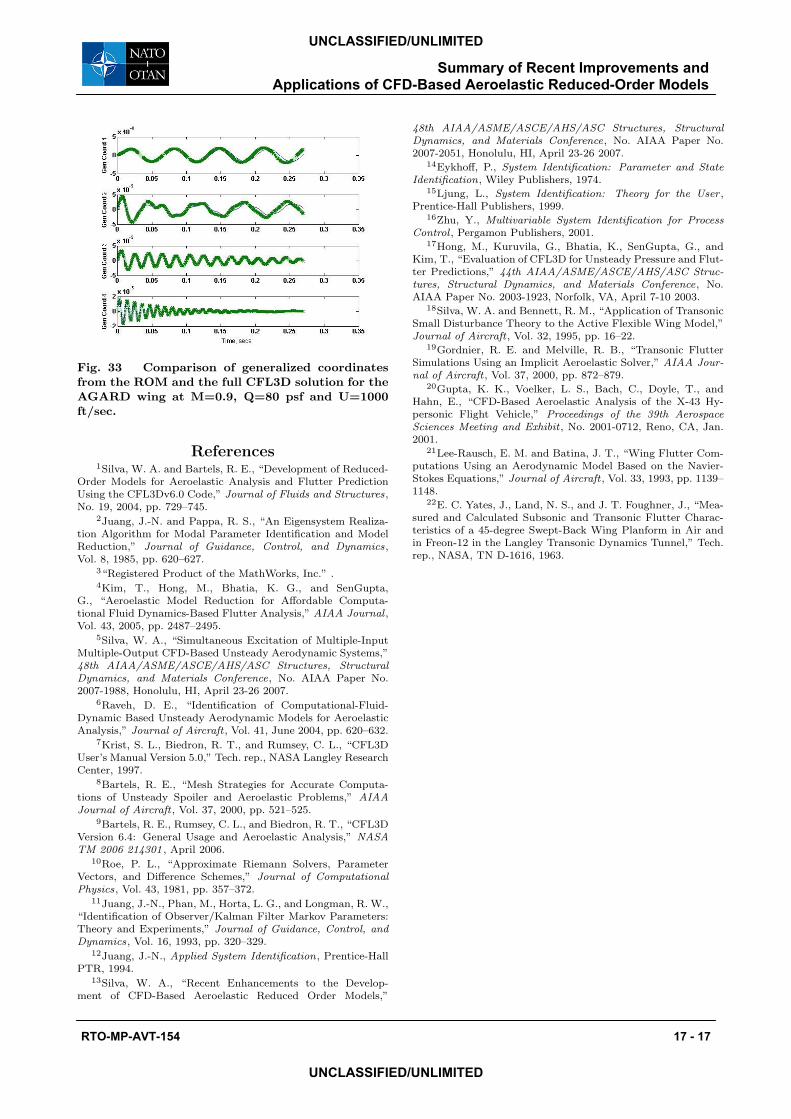
Likewise, Figure 33 presents a comparison of thegeneralized coordinate responses generated at a dy-namic pressure of 80 psf and a velocity of 1000ft/sec and the corresponding generalized coordinateresponses from the direct CFL3D solution. Onceagain, the comparison is excellent and serves to val-idate the newly-developed matched-point ROM solu-tion.

Concluding RemarksRecent enhancements to the development of aeroe-

lastic reduced-order models (ROMs) have been pre-sented. These enhancements include the capabilityto compute combined static and dynamic aeroelasticresponses and matched-point solutions using a singleROM. The simultaneous application of the structuralmodes as input to the CFD was briefly described asthe details of this enhancement were provided in aseparate paper. The ability to compute static anddynamic aeroelastic responses using the ROM waspresented. Combined static and dynamic aeroelasticresponses were computed using a ROM of the RSM

Fig. 31 Comparison of generalized coordinatesfrom the ROM and the full CFL3D solution forthe AGARD wing at M=0.9, Q=75 psf and U=973ft/sec.

Fig. 32 Comparison of generalized coordinatesfrom the ROM and the full CFL3D solution forthe AGARD wing at M=0.9, Q=70 psf and U=400ft/sec.

supersonic configuration. These combined responseswere compared with similar responses from the CFL3Dcode. The comparisons indicated reasonable correla-tion, depending on the dynamic pressure of interest.Additional research is underway to identify the sourceof some discrepancies as well as to optimize the overallprocess. Finally, the matched-point solution enhance-ment was shown to accurately compute aeroelasticresponses of a given ROM of the AGARD 445.6 wing atvarious dynamic pressures and velocities. These newenhancements to the development of aeroelastic ROMsprovides a significant advancement in ROM technol-ogy and enables the practical and efficient applicationof ROM technology to real-world problems.


RTO-MP-AVT-154 17 - 17



Fig. 33 Comparison of generalized coordinatesfrom the ROM and the full CFL3D solution for theAGARD wing at M=0.9, Q=80 psf and U=1000ft/sec.

References1Silva, W. A. and Bartels, R. E., “Development of Reduced-

Order Models for Aeroelastic Analysis and Flutter PredictionUsing the CFL3Dv6.0 Code,” Journal of Fluids and Structures,No. 19, 2004, pp. 729–745.

2Juang, J.-N. and Pappa, R. S., “An Eigensystem Realiza-tion Algorithm for Modal Parameter Identification and ModelReduction,” Journal of Guidance, Control, and Dynamics,Vol. 8, 1985, pp. 620–627.

3“Registered Product of the MathWorks, Inc.” .4Kim, T., Hong, M., Bhatia, K. G., and SenGupta,

G., “Aeroelastic Model Reduction for Affordable Computa-tional Fluid Dynamics-Based Flutter Analysis,” AIAA Journal ,Vol. 43, 2005, pp. 2487–2495.

5Silva, W. A., “Simultaneous Excitation of Multiple-InputMultiple-Output CFD-Based Unsteady Aerodynamic Systems,”48th AIAA/ASME/ASCE/AHS/ASC Structures, StructuralDynamics, and Materials Conference, No. AIAA Paper No.2007-1988, Honolulu, HI, April 23-26 2007.

6Raveh, D. E., “Identification of Computational-Fluid-Dynamic Based Unsteady Aerodynamic Models for AeroelasticAnalysis,” Journal of Aircraft , Vol. 41, June 2004, pp. 620–632.

7Krist, S. L., Biedron, R. T., and Rumsey, C. L., “CFL3DUser’s Manual Version 5.0,” Tech. rep., NASA Langley ResearchCenter, 1997.

8Bartels, R. E., “Mesh Strategies for Accurate Computa-tions of Unsteady Spoiler and Aeroelastic Problems,” AIAAJournal of Aircraft , Vol. 37, 2000, pp. 521–525.

9Bartels, R. E., Rumsey, C. L., and Biedron, R. T., “CFL3DVersion 6.4: General Usage and Aeroelastic Analysis,” NASATM 2006 214301 , April 2006.

10Roe, P. L., “Approximate Riemann Solvers, ParameterVectors, and Difference Schemes,” Journal of ComputationalPhysics, Vol. 43, 1981, pp. 357–372.

11Juang, J.-N., Phan, M., Horta, L. G., and Longman, R. W.,“Identification of Observer/Kalman Filter Markov Parameters:Theory and Experiments,” Journal of Guidance, Control, andDynamics, Vol. 16, 1993, pp. 320–329.

12Juang, J.-N., Applied System Identification, Prentice-HallPTR, 1994.

13Silva, W. A., “Recent Enhancements to the Develop-ment of CFD-Based Aeroelastic Reduced Order Models,”

48th AIAA/ASME/ASCE/AHS/ASC Structures, StructuralDynamics, and Materials Conference, No. AIAA Paper No.2007-2051, Honolulu, HI, April 23-26 2007.

14Eykhoff, P., System Identification: Parameter and StateIdentification, Wiley Publishers, 1974.

15Ljung, L., System Identification: Theory for the User ,Prentice-Hall Publishers, 1999.

16Zhu, Y., Multivariable System Identification for ProcessControl , Pergamon Publishers, 2001.

17Hong, M., Kuruvila, G., Bhatia, K., SenGupta, G., andKim, T., “Evaluation of CFL3D for Unsteady Pressure and Flut-ter Predictions,” 44th AIAA/ASME/ASCE/AHS/ASC Struc-tures, Structural Dynamics, and Materials Conference, No.AIAA Paper No. 2003-1923, Norfolk, VA, April 7-10 2003.

18Silva, W. A. and Bennett, R. M., “Application of TransonicSmall Disturbance Theory to the Active Flexible Wing Model,”Journal of Aircraft , Vol. 32, 1995, pp. 16–22.

19Gordnier, R. E. and Melville, R. B., “Transonic FlutterSimulations Using an Implicit Aeroelastic Solver,” AIAA Jour-nal of Aircraft , Vol. 37, 2000, pp. 872–879.

20Gupta, K. K., Voelker, L. S., Bach, C., Doyle, T., andHahn, E., “CFD-Based Aeroelastic Analysis of the X-43 Hy-personic Flight Vehicle,” Proceedings of the 39th AerospaceSciences Meeting and Exhibit , No. 2001-0712, Reno, CA, Jan.2001.

21Lee-Rausch, E. M. and Batina, J. T., “Wing Flutter Com-putations Using an Aerodynamic Model Based on the Navier-Stokes Equations,” Journal of Aircraft , Vol. 33, 1993, pp. 1139–1148.

22E. C. Yates, J., Land, N. S., and J. T. Foughner, J., “Mea-sured and Calculated Subsonic and Transonic Flutter Charac-teristics of a 45-degree Swept-Back Wing Planform in Air andin Freon-12 in the Langley Transonic Dynamics Tunnel,” Tech.rep., NASA, TN D-1616, 1963.


17 - 18 RTO-MP-AVT-154



Documents

Summary of Recent Improvements and Applications … Meeting...Summary of Recent Improvements and Applications of CFD-Based Aeroelastic Reduced-Order Models 17 - 2 RTO-MP-AVT-154 UNCLASSIFIED/UNLIMITED