Summary and response evidence of David Fox (statistics for turbidity triggers)

Dated: 28 April 2017

REFERENCE: JM Appleyard (jo.appleyard@chapmantripp.com)

ML Nicol (michelle.nicol@chapmantripp.com)

Before Hearing Commissioners

at Christchurch

under: the Resource Management Act 1991

in the matter of: applications CRC172455, CRC172522, CRC172456, and

CRC172523 to undertake channel deepening dredging

and maintenance dredging in Lyttelton Harbour

and

in the matter of: Lyttelton Port Company Limited

Applicant

1

100081355/967552.2

SUMMARY AND RESPONSE EVIDENCE OF DAVID FOX

INTRODUCTION

1 My name is David Fox.

2 I prepared evidence dated 28 March 2017 for Lyttelton Port

Company Limited (LPC) in relation to its applications for resource

consent to undertake works known as the Channel Deepening

Project (CDP).

3 My qualifications and experience are as outlined in that evidence.

SCOPE OF EVIDENCE

4 I will present on my evidence as filed at the hearing. This brief is

limited to evidence in response to that filed by Daniel Pritchard for

Te Hapū o Ngāti Wheke, Te Rūnanga o Koukourārata, Ngāi Tahu

Seafood and Te Runanga o Ngāi Tahu (Ngāi Tahu).

5 The specific points I respond to relate to:

5.1 The statistical method for setting trigger values;

5.2 Adequacy of the baseline monitoring report;

5.3 Statistical methods to harmonise modelled total suspended

solids (TSS) concentrations with measured turbidity;

5.4 Implementation of the modified Intensity Frequency Duration

(m-IFD) approach; and

5.5 Attribution of turbidity exceedance events to natural causes.

RESPONSE EVIDENCE

The statistical method for setting trigger values

6 Dr Pritchard claims at paragraph 14 of his evidence that there has

been “an apparent misinterpretation by LPC of the statistical method

for setting trigger values and the implications of this for adaptive

management”.

7 I concede that the proposed method for monitoring and managing

turbidity levels during the proposed dredging activities represents

‘new thinking’ and as such represents a technical advancement on

similar methods used in other international dredging projects – and

in particular those in Australia and New Zealand.

2

100081355/967552.2

8 Any initial ambiguity or lack of specificity as the technical detail was

being worked through should not be used, however, to undermine

the credibility of the process or of the proposed method. The

methodology proposed for calculating trigger values is robust and

appropriate for use in this project, and I note that view is shared by

Mr Dougal Greer who completed a report on which the section 42A

Officer’s report relied.1

9 Dr Pritchard’s more substantive comments regarding the

development of trigger values is covered in paragraphs 83 to 98 of

his evidence. My responses to pertinent issues are summarised as

follows.

10 At paragraph 86 Dr Pritchard says he has significant questions

around how the m-IFD approach will work in practice. In response, I

have prepared an additional Technical Note titled “Implementation

of a modified IFD approach for turbidity monitoring”, dated 18 April

2017 (Technical Note).

11 That Technical Note is appended to this evidence, and in brief,

provides:

11.1 A working definition of a turbidity exceedance;

11.2 Technical explanation as to why it is necessary to

parameterise the m-IFD methodology based on an analysis of

background turbidity data augmented with predicted dredge

TSS; and

11.3 Details as to how the m-IFD approach will be implemented in

practice.

12 At paragraph 87 Dr Pritchard seems to be inferring that the use of

modelled TSS concentrations in the establishment of parameters for

the m-IFD method was less than transparent. In response I note:

12.1 My involvement in the CDP commenced with my first

attendance at meeting 13 of the TAG on 28 June 2016 so I

cannot comment on TAG deliberations prior to that time;

12.2 However, as mentioned above, the science of setting trigger

values leading to the m-IFD approach has evolved as a result

of my engagement on the project and adjustments in strategy

are part of that evolution;

12.3 The use of both background and modelled turbidity data was

articulated in my initial report “Recommended data

1 See paragraph 256 of the Officer’s report,

3

100081355/967552.2

processing and Trigger-Value methods for the LPC CDP” which

stated: “Trigger values will utilise monitored data …

augmented with the incremental turbidity due to dredging as

predicted by LPC’s hydrodynamic modelling”; and

12.4 This document was dated 16 September 2016 and the ideas

underpinning it had been floated prior to that time.

13 At paragraphs 89 and 90 Dr Pritchard questions the rationale for

using both background and modelled turbidity in setting trigger

values. I have provided further explanation of why there is a need

to use both background and modelled turbidity when using the

three, related concepts of exceedance intensity, frequency, and

duration in the Technical Note appended to this evidence.

14 Briefly, the Technical Note outlines the logic which compels us to

use both background and modelled turbidity when setting the

operational parameters of the m-IFD approach.

Adequacy of the baseline monitoring report

15 The issue of an ‘appropriate’ baseline monitoring period has been

extensively discussed and, as noted by Dr Pritchard at paragraph 71

of his evidence the one year time-frame adopted for this project

represented a “consensus view” of the TAG.

16 Dr Pritchard does ‘not disagree’ that one year of monitoring is

“adequate” for setting trigger values, but suggests that the consent

conditions “should allow for a longer period of baseline data

collection, if such an opportunity arises”.

17 Leaving aside issues of academic curiosity versus commercial

imperitives, I note that the one year baseline data collection

program is ‘balanced’ to the extent that all months and seasons are

represented. An additional few weeks or months of background data

will distort this balance. A counter to this suggestion is that a further

year of baseline data collection be undertaken. My response to such

a suggestion is that in the absence of a compelling scientific

argument, this ‘more is better’ view has no basis in either fact or

evidence. This issue was addressed in my original report.

Statistical methods to harmonise modelled total suspended

solids (TSS) concentrations with measured turbidity

18 Dr Pritchard devotes several paragraphs (93 – 98) to the discussion

of statistical issues associated with the reconciliation of predicted

turbidity from hydrodynamic models which are expressed as

concentrations having units mgL-1 with empirical data expressed in

nephelometric turbidity units (NTU).

4

100081355/967552.2

19 I strongly disagree with Dr Pritchard’s claim at paragraph 93 that

“there is no agreement on the method to convert modelled

suspended sediment concentrations (units: mg/L) to the same units

as measured turbidity (Nephelometric Turbidity Units, NTU)”.

20 While the precise form of the relationship would be influenced both

by the data at hand and preferences of the modeller, I am confident

in asserting that any realistic model would be drawn from the class

of general linear (statistical) models. In my experience, the TSS-

NTU relationship is highly linear within the range of normal

turbidities encountered in the system being modelled (and I note Dr

Pritchard actually appears to share this view from his statement in

paragraph 94).

21 Dr Pritchard introduces additional doubt about the TSS-NTU

modelling in subsequent paragraphs (95 – 97) by questioning

whether the fitted model should have a zero or non-zero intercept. I

do not dispute this could be an important consideration, but based

on the analyses undertaken to date, it is inconsequential.

22 Dr Pritchard refers to discussions at the 7 March 2017 TAG meeting.

I led those discussions and presented detailed results of the model-

fitting exercise. This included preliminary model parameter

estimates of the intercept and slope terms of 1.33 and 0.415

respectively for the relationship between NTU and TSS. Thus, the

model assigns an NTU of 1.33 to a modelled TSS of 0 mgL-1. In the

context of recent ‘natural’ turbidity readings as high as 180 NTU

(Site UH1, 22-Jan-2017 15:30) this 1.33 NTU off-set is of no

statistical or ecological relevance.

23 While I agree that conceptually a model having a zero intercept

makes more sense (and this can be implemented when the

complete data set is analysed), this would not have had any

material impact on the analyses or conclusions presented to date.

Implementation of the modified Intensity Frequency

Duration (m-IFD) approach

24 In his evidence, Dr Pritchard notes “significant concerns” with the

implementation of the m-IFD approach - particularly those relating

to:

24.1 the definition of an exceedance ‘event’;

24.2 the interplay between exceedance durations and frequency;

24.3 quantification of event probabilities; and

24.4 the opportunity for perverse outcomes.

5

100081355/967552.2

25 The incremental development of the m-IFD approach has provided

opportunity for LPC, the TAG, ECan and interested stakeholders to

‘stress-test’ the methodology. This is an important part of the

consent process that will ensure the adopted strategy is robust and

fit-for-purpose.

26 My recent Technical Note addresses Dr Pritchard’s concerns listed

above. A summary of responses follows.

Definition of an exceedance ‘event’

27 An exceedance event is now simply defined as any instance for

which the recorded turbidity (NTU) exceeds an intensity threshold

(also referred to the trigger-value).

Interplay between exceedance duration and frequency

28 The total of all exceedance durations in a reporting period shall not

exceed a limit based on the intensity level used in the definition of

an exceedance event. Individual limits on exceedance duration and

exceedance frequency are not required since they are implicitly

controlled by the limit on total exceedance duration.

Quantification of event probabilities

29 Dr Pritchard correctly identified the need to quantify the overall

exceedance probability when an earlier definition of an exceedance

event was used. For completeness, this conditional probability

calculation has been undertaken and details are available in my

Technical Note. However, the revised definition of ‘exceedance

event’ given above together with the limit imposed by the interplay

between exceedance duration and frequency renders this calculation

obsolete.

Opportunity for perverse outcomes

30 An issue raised in the last TAG meeting and mentioned again in Dr

Pritchard’s evidence concerned the possibility of perverse and

unwanted outcomes using the previously described m-IFD approach.

In particular, when using a mechanism based on total number of

exceedances and the average duration of those exceedances,

turbidity could be maintained at an unacceptably high level following

the tripping of a turbidity trigger until the end of the reporting

period. This situation was provided by Dr Pritchard as an example of

an “absurdity” that could have arisen under the previous formulation

of the m-IFD approach.

31 Such absurdities cannot arise using the revised definition of

‘exceedance event’ given above together with the limit imposed by

the interplay between exceedance duration and frequency.

6

100081355/967552.2

Attribution of turbidity exceedance events to natural causes

32 My original report included as Appendix 20 to the Applications

outlined statistical methods I developed during Gladstone Port

Corporation’s Western Basin Dredging Project to provide managers

and regulators with a tool to ‘decompose’ measured turbidity into

‘natural’ and dredge-derived componentsLPC are aware of this

capability although contrary to Dr Pritchard’s claim in paragraph

115, there has been no commitment to develop it for LPC’s CDP.

Dated: 28 April 2017

__________________________

David Fox

Technical Note

Implementation of a modified IFD approach for turbidity monitoring

David R. Fox, PhD.,C.Stat.,P.Stat.,C.Sci.

Equivalence of Time-based sampling and Event-based sampling

In considering various options and amendments to the so-called IFD approach to turbidity

monitoring and triggering, it is important to understand the intimate nexus between time-based

sampling and event-based sampling. This concept is related to stationary ergodic processes in time-

series analysis. An ergodic process is one which conforms to the ergodic theorem which can be

stated as:

the time average of a conforming process to equal the ensemble average. In

practice this means that statistical sampling can be performed at one

instant across a group of identical processes or sampled over time on a

single process with no change in the measured result.

Source: https://en.wikipedia.org/wiki/Stationary_ergodic_process

These concepts are illustrated in Figure 1.

Figure 1. Illustration of ergodic principle showing equivalence of mean obtained by averaging many realisations of an underlying process at a single time (left) or averaging a single realisation of the process over a long time (right).

In the case of turbidity monitoring, we sample a continuously evolving signal at regular, discrete

points in time (Figure 2).

Figure 2. Depiction of a continuous turbidity signal and sampling at regular intervals in time. Time increment is Δt. Horizontal red line placed at some percentile, Yα (also referred to as the intensity level) is such that α·100% of all turbidity values are less than or equal to Yα or equivalently, (1-α)·100% of all turbidity values are greater than Yα.

We can reduce Figure 2 to a binary sequence using an indicator function, Z t to indicate when the

turbidity signal is either above or below Y as follows:

1 if

0 otherwise

Y t YZ t

(1)

This generates a “pulsed”” signal as shown in Figure 3.

Referring to the bottom plot in Figure 3, the fraction of time the turbidity signal is aboveY ( 1 )

is represented by the total of the shaded areas out of the total area ( )T . Expressed

mathematically, this is:

0

11 ( )

T

Z t dtT

(2)

For the discrete sampling of the continuous turbidity signal represented by the top plot in Figure 3

we divide the time-period [0, ]T into n equal time increments each of length t . That is:

Tt

n (3)

Figure 3. Reduction of continuous signal Y(t) to a binary signal, Z(t).

Now, the total of the shaded areas in the lower plot in Figure 3 is approximately 1

n

j

j

Z t

and

substituting this in the right-hand side of Equation 2 gives us:

1

11

n

j

j

Z tT

(4)

Furthermore, from Equation 3, T n t and substituting this into Equation 4 gives:

Z(t)

t0

1

T

X1 X2 X3 Xk

Exceedance durations

11

n

j

j

Z

n

(5)

But 1

n

j

j

Z

is simply the number of times ( )Y t Y ( , say)k and so Equation 5 becomes:

1k

n (6)

Now the approximation in Equation 4 improves as ( t 0)n implying

0

1( ) as

TkZ t dt n

n T .

But 0

( )T

Z t dt is equivalent to the total exceedance time (depicted as 1 2, , , kX X X in the top plot

of Figure 3.

So finally, we have:

1 (1 )

k

i

i

Xk

n T

(7)

which establishes that the fraction of discrete exceedance events is equivalent (in the limit as

0t ) to the proportion of time the trigger value is exceeded where that proportion is used to

identify the trigger value, Y .

Establishing the case for a modified IFD Approach

The IFD approach is based on the three related concepts of the intensity of an exceedance; the

frequency of an exceedance; and the duration of an exceedance. As detailed in Fox (2016), previous

implementations of this methodology in other dredging projects have unwittingly perturbed the

assumed exceedance rate by treating these three exceedance attributes as independent quantities

to be manipulated at will. In fact, specification of any two components completely determines the

third. This follows immediately from Equation 7 since:

1

1

(1 ) = (1 )

(1 )

k

i ki

i

i

X

X TT

k X T

(8)

We see from Equation 8 that specification of the intensity level ( ) and the frequency (k) say, means

that the average duration must satisfy 1 T

Xk

.

Or equivalently that the total exceedance duration (of all exceedances in the time period 0,T )

must be (1 ) T .

There is an important corollary associated with these results and that concerns the use of either the

historical record of background (‘natural’) turbidity only to set the parameters of the IFD approach

or a scheme based on the background data plus the additional turbidity due to dredging.

A scheme based on only the background data in effect makes no provision for the proposed

dredging activity – the ambient or background turbidity signal will exceed any nominated intensity

threshold with frequencies and durations that honour Equation 8. Thus, under this scheme and to

remain ‘compliant’, there can be no perturbation of the background signal.

The need to include the effects of modelled or predicted turbidity arising from the dredging activity

is reasoned as follows:

(i) Dredging (temporarily) increases turbidity and that increase has been quantified;

(ii) Approval of the project gives license to (i);

(iii) Alteration of the background turbidity signal means the I, F, and D components of

turbidity exceedances cannot simultaneously honour those derived from an analysis

of the background turbidity data alone;

(iv) The I, F, and D components of turbidity exceedances need to be adjusted to capture

the characteristics of the modified turbidity signal and to place limits on those

components in a manner that:

a. acknowledges the dependencies among all three components; and

b. ensures that the more extreme turbidity events during dredging are within the

limits of what has been predicted.

Definition of an exceedance event

The notion of ‘compliance’ is inextricably linked to that of ‘exceedance’ with the former determined

from an analysis of the latter. What constitutes an ‘exceedance event’ requires careful definition so

that determinations of compliance status are both meaningful and accurate.

Two possibilities for determining exceedance events are discussed below.

A. ID Events

This definition uses the dual concepts of intensity and duration to define an exceedance event. An ID

event is deemed to have occurred when the following two conditions have occurred:

A.1 the turbidity reading (or other metric derived from it), ( )Y t exceeds the intensity

trigger at the (1 )100% level. This latter quantity is denoted 1

Y

; and

A.2 the length of continuous time that A.1 is satisfied is greater than a threshold

duration for that intensity level, *X .

An immediate consequence of this definition is that the actual exceedance rate (call it ) will be

smaller than the assumed exceedance rate, . To overcome this, an adjustment ( = increase) to the

nominal intensity trigger level is required. The details are provided below.

Definitions

( )Y t is the (smoothed) turbidity level at time t;

is the nominal exceedance rate used to set the intensity trigger 1

Y

;

*X is the threshold duration at intensity level (1 )100% ;

( )

iX

is the observed duration of the ith triggering event; and

; ,X

xF is the cumulative distribution function of the ( )

iX

with parameter vector .

Mathematically, A.1 and A.2 above can be stated as:

1 1( )A Y t Y

and 2

( ) *

iA X X

(9)

and an ID event as:

( )

1 2

IDE A A (10)

From elementary probability theory:

( )

1 2 2 2 1 1

IDP E P A A P A P A A P A (11)

where P denotes a conditional probability.

Now 1P A (by definition) and hence Equation 11 reduces to:

( )

2 1

IDP E P A A (12)

Also by definition, 2 1

*1 XP A A F x , thus the unconditional probability of exceedance ( ) is:

*1 XF x

(13)

Equation 13 can be used to adjust the intensity trigger so that the unconditional probability of

exceedance, is some pre-determined value.

For example, suppose *X is set equal to the median of all durations at intensity level and

therefore *1 0.5

XF x

. Making this substitution in Equation 13 we see that for an overall

exceedance rate of 0.05 the intensity level needs to be set to 0.10.

The implication of this adjustment is that event 1A occurs more frequently but this is attenuated by

the additional requirement that the duration must be at least *X time units before an exceedance is

declared.

Comment

The implementation of the ID definition is somewhat problematic and still lacks integration of the F

component, that is how many ID events are permitted during the observational period?

Furthermore, it remains to be decided how to treat durations associated with the event 1 2A A

which in words is the event that the intensity trigger was tripped but the duration did not exceed the

critical threshold *X . Under this scenario, since an ID-event did not occur, no exceedance duration

is recorded.

Finally, and without further modification, the possibility for perverse outcomes could arise. For

example, dredging operations could continue from the time an ID-event occurred to the end of the

reporting period to limit the number of ID events.

We believe there is a simpler, more effective alternative which simultaneously utilises all three

dimensions of the IFD approach while avoiding the need to make adjustments of the form given by

Equation 13.

B. IFD Events

It has been argued above that the mechanics of any IFD approach need to be determined from an

analysis of historical background data plus the anticipated contribution due to the dredging activity.

We have also noted that the use of ID events as described above exposes dredging operators to

claims of manipulating turbidity levels once an ID event is established to minimise the total number

of exceedance events. We hasten to add that this runs counter to the notion of environmental

protection and would simply not happen. However, the systems and procedures that are ultimately

adopted must not only be scientifically robust but must also be resilient to any claimed short-

comings. To this end, we describe an approach which couples all three components (intensity;

frequency; and duration) using the previously established equivalence between time-based sampling

and event-based sampling.

The essence of the procedure is the recognition that the fraction of time in an exceedance state

must be no greater than - the level used to determine the intensity trigger for discrete event

sampling. Since it is the product of both frequency and (average) duration which determines the

total exceedance time, these two components do not need to be separately managed – only the

total time.

For example, suppose the reporting period is 30 days or 720 hours. Using an intensity trigger based

on the 95th. percentile of the turbidity data implies that only 5% of turbidity readings will exceed this

level (assuming an ‘in-control’ process). Equivalently, the total time that turbidity exceeds this

trigger can be no more than 36 hours. The composition of exceedance events contributing to this 36-

hour duration limit is somewhat immaterial – it could be due to many short-duration exceedances, a

small number of long exceedances or, as is more likely, a range of durations.

Implementation and management of this system is very simple having only two steps:

1. For a chosen intensity level (1 ) determine the intensity trigger, 1Y ;

2. For a fixed monitoring interval 0,T set a limit on the cumulative exceedance time

equal to T .

A management response is required when the limit in 2 above has been (or is about to be)

exceeded.

The only other matters requiring consideration are: (i) the value ofT ; and (ii) whether the reporting

period 0,T is a fixed or moving window. These are management decisions that need to be

informed by the ecology of the system. In both the Port Phillip Bay Channel Deepening project and

Gladstone Port’s Western Basin Dredging project where the primary aim was the protection of

seagrass meadows, a 2-week moving window was used.

Unless there are compelling ecological reasons to do otherwise, we suggest that a 2-week time

frame would also be appropriate for the LPC CDP. The difficulty with moving windows of longer

duration is a ‘persistence’ effect – that is, the dominance of a single exceedance of long duration

persisting for at least T time units.

These issues are explored with an example using monitored data from site SG2.

Example

Measured turbidity at site SG2 for the period September 2016 to February 2017 is shown in Figure 4.

The 95th. intensity trigger is determined to be 23.3 NTU. The impact of natural weather events in

January 2017 is evident from Figure 4 with a single 39-hour exceedance event commencing at 8am

on January 22 and running until 11pm the following day.

Using a 30-day moving window requires the cumulative exceedance time in any preceding 30-day

period not exceeding 36 hours (when using trigger corresponding to the 95th. intensity level). Thus,

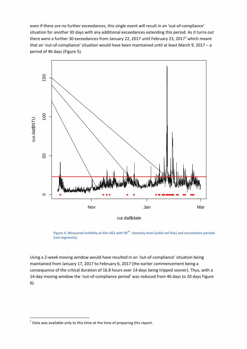
even if there are no further exceedances, this single event will result in an ‘out-of-compliance’

situation for another 30 days with any additional exceedances extending this period. As it turns out

there were a further 30 exceedances from January 22, 2017 until February 23, 20171 which meant

that an ‘out-of-compliance’ situation would have been maintained until at least March 9, 2017 – a

period of 46 days (Figure 5).

Figure 4. Measured turbidity at Site SG2 with 95th

. intensity level (solid red line) and exceedance periods (red segments).

Using a 2-week moving window would have resulted in an ‘out-of-compliance’ situation being

maintained from January 17, 2017 to February 6, 2017 (the earlier commencement being a

consequence of the critical duration of 16.8 hours over 14 days being tripped sooner). Thus, with a

14-day moving window the ‘out-of-compliance period’ was reduced from 46 days to 20 days Figure

6).

1 Data was available only to this time at the time of preparing this report.

Nov Jan Mar

05

01

00

15

0

cur.dat$date

cu

r.d

at$

NT

U

Figure 5. Remaining exceedance hours at site SG2 using a 30-day moving ‘compliance’ window.

Figure 6. Remaining exceedance hours at site SG2 using a 14-day moving ‘compliance’ window.

1/03

/201

7

21/0

2/20

17

11/0

2/20

17

1/02

/201

7

21/0

1/20

17

11/0

1/20

17

1/01

/201

7

21/1

2/20

16

11/1

2/20

16

1/12

/201

6

25

20

15

10

5

0

Exce

ed

an

ce h

ou

rs r

em

ain

ing

1/03

/201

7

21/0

2/20

17

11/0

2/20

17

1/02

/201

7

21/0

1/20

17

11/0

1/20

17

1/01

/201

7

21/1

2/20

16

11/1

2/20

16

1/12

/201

6

21/1

1/20

16

11/11/

2016

9

8

7

6

5

4

3

2

1

0

Exce

ed

an

ce h

ou

rs r

em

ain

ing

REFERENCE

Fox, D.R. 2016. Statistical considerations associated with the establishment of turbidity triggers: Candidate methodologies for large-scale dredging projects. Environmetrics Australia Technical Report, 16 September 2016.

April 18, 2017

Additional Considerations – April 22, 2017 A new concept has been introduced to explain the use of background + dredge for setting parameters of the m-IFD approach. This is outlined below:

After further consideration, the ‘IFD-Equivalence Theorem’ is not strictly correct. The reason for this

is that the m-IFD only looks at exceedances over a threshold – it makes no difference whether the

exceedance is by 1 NTU of 10,000 NTU. However, the magnitudes exceedances will be instrumental

in determining other properties such as mean, variance etc.

These concepts are explored in greater detail below.

Figure 7. Lognormal(2.441,0.5124,0.0) distribution of background NTU (blue) and lognormal(2.5,0.3,26.67) dredge contribution (red).

Figure 8. Lognormal(2.441,0.5124,0.0) distribution of background NTU (blue) and lognormal(4.0,0.3,,26.67) dredge contribution (red).

200150100500

0.10

0.08

0.06

0.04

0.02

0.00

NTU

pro

b. d

en

sity

200150100500

0.10

0.08

0.06

0.04

0.02

0.00

NTU

pro

b. d

en

sity

Figure 9. Simulated NTU time-series of NTU data for background only (top); background plus dredge contribution corresponding to Figure 7 (middle); and background plus dredge contribution corresponding to Figure 8 (bottom).

Comment The three time-series in Figure 9 have identical IFD characteristics: the 95th. percentile in all three

cases is 26.67. In fact, all percentiles 95P will be identical and all percentiles 95P

different. Statistics for background turbidity and (1) middle series in Figure 9; and (2) bottom series in Figure 9 are given in Table 1. Table 1. Statistics for the three time-series in Figure 9.

Variable N N* Mean SE Mean StDev Minimum Q1 Median Q3 Maximum

B/g NTU 15148 0 13.085 0.0590 7.268 1.452 8.083 11.380 16.178 104.764

(1) 15148 0 13.722 0.0763 9.385 1.452 8.083 11.380 16.178 118.208

(2) 15148 0 15.955 0.151 18.550 1.452 8.083 11.380 16.178 175.146

Now, the mean NTU is a measure of turbidity load. We see that for series (1) the mean has increased 5% above background while for series (2) it has increased 22%. It is relatively easy to work out what the mean dredge NTU needs to be (when dredging is managed using m-IFD) so that the increase in overall turbidity load is kept to some required level. This mean dredge NTU can be expressed as a multiple of the mean of the background NTU (Table 2). For example, if we implemented an m-IFD program based on an intensity level of 95% and consent was given to increase overall sediment load by 25%, then the mean NTU for the dredge input would be six-times the mean background NTU provided the patterns of turbidity exceedance did not violate the limits imposed by the m-IFD program. From Table 1 the background NTU is 13.085 so the mean dredge NTU would be set at 78.5 NTU.

200

100

0

200

100

0

01-Mar-201701-Feb-201701-Jan-201701-Dec-201601-Nov-201601-Oct-2016

200

100

0

X

P95

X+W1

P95

X+W2

P95

Table 2. Multipliers of mean background turbidity for computing mean dredge turbidity levels to be maintained while using m-IFD with specified intensity level for various increases in overall sediment load.

Intensity level

Increase in sediment load

(%) 0.8 0.85 0.9 0.95 0.975 0.99

5 1.3 1.3 1.5 2.0 3.0 6.0

10 1.5 1.7 2.0 3.0 5.0 11.0

15 1.8 2.0 2.5 4.0 7.0 16.0

20 2.0 2.3 3.0 5.0 9.0 21.0

25 2.3 2.7 3.5 6.0 11.0 26.0

30 2.5 3.0 4.0 7.0 13.0 31.0

35 2.8 3.3 4.5 8.0 15.0 36.0

40 3.0 3.7 5.0 9.0 17.0 41.0

45 3.3 4.0 5.5 10.0 19.0 46.0

50 3.5 4.3 6.0 11.0 21.0 51.0

55 3.8 4.7 6.5 12.0 23.0 56.0

60 4.0 5.0 7.0 13.0 25.0 61.0

65 4.3 5.3 7.5 14.0 27.0 66.0

70 4.5 5.7 8.0 15.0 29.0 71.0

75 4.8 6.0 8.5 16.0 31.0 76.0

80 5.0 6.3 9.0 17.0 33.0 81.0

85 5.3 6.7 9.5 18.0 35.0 86.0

90 5.5 7.0 10.0 19.0 37.0 91.0

95 5.8 7.3 10.5 20.0 39.0 96.0

100 6.0 7.7 11.0 21.0 41.0 101.0

Conclusion At the risk of increasing complexity, the m-IFD really needs to incorporate another dimension so that not only are the patterns of exceedances controlled, but also the magnitudes. Because of the relationship to overall sediment load, it is suggested that a further control be imposed on the mean turbidity of the dredge contribution.