Embed Size (px)
Citation preview
SUBMITTED TO IEEE TRANSACTIONS ON IMAGE PROCESSING, VOL. XX, NO. XX, XX 1
Statistics of Deep Generated ImagesYu Zeng, Huchuan Lu, and Ali Borji
Abstract—Here, we explore the low-level statistics of imagesgenerated by state-of-the-art deep generative models. First,Variational auto-encoder (VAE [19]), Wasserstein generativeadversarial network (WGAN [2]) and deep convolutional gen-erative adversarial network (DCGAN [23]) are trained on theImageNet dataset and a large set of cartoon frames fromanimations. Then, for images generated by these models aswell as natural scenes and cartoons, statistics including meanpower spectrum, the number of connected components in a givenimage area, distribution of random filter responses, and contrastdistribution are computed. Our analyses on training imagessupport current findings on scale invariance, non-Gaussianity,and Weibull contrast distribution of natural scenes. We findthat although similar results hold over cartoon images, thereis still a significant difference between statistics of natural scenesand images generated by VAE, DCGAN and WGAN models. Inparticular, generated images do not have scale invariant meanpower spectrum magnitude, which indicates existence of extrastructures in these images caused by deconvolution operations.We also find that replacing deconvolution layers in the deepgenerative models by sub-pixel convolution helps them generateimages with a mean power spectrum closer to the mean powerspectrum of natural images. Inspecting how well the statistics ofdeep generated images match the known statistical properties ofnatural images, such as scale invariance, non-Gaussianity, andWeibull contrast distribution, can a) reveal the degree to whichdeep learning models capture the essence of the natural scenes, b)provide a new dimension to evaluate models, and c) allow possibleimprovement of image generative models (e.g., via defining newloss functions).
Index Terms—generative models, image statistics, convolu-tional neural networks, deep learning.
I. INTRODUCTION AND MOTIVATION
GENERATIVE models are statistical models that attemptto explain observed data by some underlying hidden
(i.e., latent) causes [16]. Building good generative modelsfor images is very appealing for many computer vision andimage processing tasks. Although a lot of previous effort hasbeen spent on this problem and has resulted in many models,generating images that match the qualities of natural scenesremains to be a daunting task.
There are two major schemes for the design of imagegenerative models. The first one is based on the known regu-larities of natural images and aims at satisfying the observedstatistics of natural images. Examples include the GaussianMRF model [22], for the 1/f -power law, and the Dead leaves
Y. Zeng is with School of Information and Communication En-gineering at Dalian University of Technology, Dalian, China. E-mail:[email protected].
H. Lu is with School of Information and Communication Engi-neering at Dalian University of Technology, Dalian, China. E-mail:[email protected].
A. Borji is with the Center for Research in Computer Vision and ComputerScience Department at the University of Central Florida, Orlando, [email protected]
Manuscript received xx 2017.
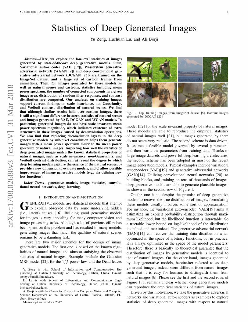
Fig. 1. Top: training images from ImageNet dataset [5]. Bottom: imagesgenerated by DCGAN [23].
model [32] for the scale invariant property of natural images.These models are able to reproduce the empirical statisticsof natural images well [21], but images generated by themdo not seem very realistic. The second scheme is data-driven.It assumes a flexible model governed by several parameters,and then learns the parameters from training data. Thanks tolarge image datasets and powerful deep learning architectures,the second scheme has been adopted in most of the recentimage generation models. Typical examples include variationalautoencoders (VAE)[19] and generative adversarial networks(GAN)[14]. Utilizing convolutional neural networks [20], asbuilding blocks, and training on tens of thousands of images,deep generative models are able to generate plausible images,as shown in the second row of Figure 1.
On the one hand, despite the promise of deep generativemodels to recover the true distribution of images, formulatingthese models usually involves some sort of approximation.For instance, the variational auto-encoder (VAE)[19] aims atestimating an explicit probability distribution through maxi-mum likelihood, but the likelihood function is intractable. Soa tractable lower bound on log-likelihood of the distributionis defined and maximized. The generative adversarial network(GAN)[14] can recover the training data distribution whenoptimized in the space of arbitrary functions, but in practice,it is always optimized in the space of the model parameters.Therefore, there is basically no theoretical guarantee that thedistribution of images by generative models is identical tothat of natural images. On the other hand, images generatedby deep generative models, hereinafter referred to as deepgenerated images, indeed seem different from natural imagessuch that it is easy for humans to distinguish them fromnatural images [6]. Please see the first and the second rows ofFigure 1. It remains unclear whether deep generative modelscan reproduce the empirical statistics of natural images.
Driven by this motivation, we take the generative adversarialnetworks and variational auto-encoders as examples to explorestatistics of deep generated images with respect to natural
arX
iv:1
708.
0268
8v3
[cs
.CV
] 3
1 M
ar 2
018
SUBMITTED TO IEEE TRANSACTIONS ON IMAGE PROCESSING, VOL. XX, NO. XX, XX 2
images in terms of scale invariance, non-Gaussianity, andWeibull contrast distribution. These comparisons can revealthe degree to which the deep generative models capture theessence of the natural scenes and guide the community to buildmore efficient generative models. In addition, the current wayof assessing image generative models are often based on visualfidelity of generated samples using human inspections [29]. Asfar as we know, there is still not a clear way to evaluate imagegenerative models [17]. We believe that our work will providea new dimension to evaluate image generative models.
Specifically, we first train a Wasserstein generative adver-sarial network (WGAN [2]), a deep convolutional generativeadversarial network (DCGAN [23]), and a variational auto-encoder (VAE [19]) on the ImageNet dataset. The reason forchoosing ImageNet dataset is that it contains a large numberof photos from different object categories. We also collect thesame amount of cartoon images to compute their statisticsand to train the models on them, in order to: 1) comparestatistics of natural images and cartoons, 2) compare statisticsof generated images and cartoons, and 3) check whether thegenerative models work better on cartoons, since cartoons haveless texture than natural images. As far as we know, we arethe first to investigate statistics of cartoons and deep generatedimages. Statistics including luminance distribution, contrastdistribution, mean power spectrum, the number of connectedcomponent with a given area, and distribution of random filterresponses will be computed.
Our analyses on training natural images confirm existingfindings of scale invariance, non-Gaussianity, and Weibullcontrast distribution on natural image statistics. We also findnon-Gaussianity and Weibull contrast distribution in VAE,DCGAN and WGAN’s generated natural images. However,unlike real natural images, neither of the generated imageshave scale invariant mean power spectrum magnitude. Instead,the deep generative models seem to prefer certain frequencypoints, on which the power magnitude is significantly largerthan their neighborhood. We show that this phenomenon iscaused by the deconvolution operations in the deep generativemodels. Replacing deconvolution layers in the deep generativemodels by sub-pixel convolution enables them to generateimages with a mean power spectrum more similar to the meanpower spectrum of natural images.
II. RELATED WORK
In this section, we briefly describe recent work that isclosely related to this paper, including important findings inthe area of natural image statistics and recent developmentson deep image generative models.
A. Natural Image Statistics
Research on natural image statistics has been growingrapidly since the mid-1990s[16]. The earliest studies showedthat the statistics of the natural images remains the samewhen the images are scaled (i.e., scale invariance)[27], [32].For instance, it is observed that the average power spectrummagnitude A over natural images has the form of A(f) =1/f−α, α ≈ 2 (See for example [7], [4], [3], [9]). It can be
derived using the scaling theorem of the Fourier transformationthat the power spectrum magnitude will stay the same ifnatural images are scaled by a factor [33]. Several other naturalimage statistics have also been found to be scale invariant,such as the histogram of log contrasts [24], the number ofgray levels in small patches of images [11], the number ofconnected components in natural images [1], histograms offilter responses, full co-occurrence statistics of two pixels, aswell as joint statistics of Haar wavelet coefficients.
Another important property of natural image statistics is thenon-Gaussianity [27], [32], [30]. This means that marginaldistribution of almost any zero mean linear filter responseon virtually any dataset of images is sharply peaked at zero,with heavy tails and high kurtosis (greater than 3 of Gaussiandistributions) [21].
In addition to the two well-known properties of naturalimage statistics mentioned above, recent studies have shownthat the contrast statistics of the majority of natural imagesfollows a Weibull distribution [13]. Although less explored,compared to the scale invariance and non-Gaussianity of nat-ural image statistics, validity of Weibull contrast distributionhas been confirmed in several studies. For instance, Geuse-broek et al. [12] show that the variance and kurtosis of thecontrast distribution of the majority of natural images can beadequately captured by a two-parameter Weibull distribution.It is shown in [25] that the two parameters of the Weibullcontrast distribution cover the space of all possible naturalscenes in a perceptually meaningful manner. Weibull contrastdistribution also has been applied to a wide range of com-puter vision and image processing tasks. Ghebreab et al. [13]propose a biologically plausible model based on Weibullcontrast distribution for rapid natural image identification, andYanulevskaya et al. [31] exploit this property to predict eyefixation location in images, to name a few.
B. Deep Generative Models
Several deep image generative models have been proposedin a relatively short period of time since 2013. As of thiswriting, variational autoencoders (VAE) and generative adver-sarial networks (GAN) constitute two popular categories ofthese models. VAE aims at estimating an explicit probabilitydistribution through maximum likelihood, but the likelihoodfunction is intractable. So a tractable lower bound on log-likelihood of the distribution is defined and maximized. Formany families of functions, defining such a bound is possibleeven though the actual log-likelihood is intractable. In contrast,GANs implicitly estimate a probability distribution by onlyproviding samples from it. Training GANs can be described asa game between a generative model G trying to estimate datadistribution and a discriminative model D trying to distinguishbetween the examples generated by G and the ones comingfrom actual data distribution. In each iteration of training,the generative model learns to produce better fake sampleswhile the discriminative model will improve its ability ofdistinguishing real samples.
It is shown that a unique solution for G and D existsin the space of arbitrary functions, with G recovering the
SUBMITTED TO IEEE TRANSACTIONS ON IMAGE PROCESSING, VOL. XX, NO. XX, XX 3
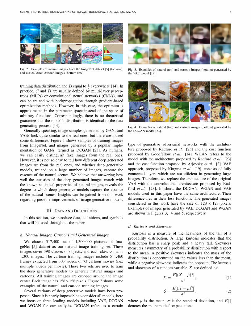
Fig. 2. Examples of natural images from the ImageNet dataset [5] (top row),and our collected cartoon images (bottom row).
training data distribution and D equal to 12 everywhere [14]. In
practice, G and D are usually defined by multi-layer percep-trons (MLPs) or convolutional neural networks (CNNs), andcan be trained with backpropagation through gradient-basedoptimization methods. However, in this case, the optimum isapproximated in the parameter space instead of the space ofarbitrary functions. Correspondingly, there is no theoreticalguarantee that the model’s distribution is identical to the datagenerating process [14].
Generally speaking, image samples generated by GANs andVAEs look quite similar to the real ones, but there are indeedsome differences. Figure 1 shows samples of training imagesfrom ImageNet, and images generated by a popular imple-mentation of GANs, termed as DCGAN [23]. As humans,we can easily distinguish fake images from the real ones.However, it is not so easy to tell how different deep generatedimages are from the real ones, and whether deep generativemodels, trained on a large number of images, capture theessence of the natural scenes. We believe that answering howwell the statistics of the deep generated images match withthe known statistical properties of natural images, reveals thedegree to which deep generative models capture the essenceof the natural scenes. Insights can be gained from this workregarding possible improvements of image generative models.
III. DATA AND DEFINITIONS
In this section, we introduce data, definitions, and symbolsthat will be used throughout the paper.
A. Natural Images, Cartoons and Generated Images
We choose 517,400 out of 1,300,000 pictures of Ima-geNet [5] dataset as our natural image training set. Theseimages cover 398 classes of objects, and each class contains1,300 images. The cartoon training images include 511,460frames extracted from 303 videos of 73 cartoon movies (i.e.,multiple videos per movie). These two sets are used to trainthe deep generative models to generate natural images andcartoons. All training images are cropped around the imagecenter. Each image has 128×128 pixels. Figure 2 shows someexamples of the natural and cartoon training images.
Several variants of deep generative models have been pro-posed. Since it is nearly impossible to consider all models, herewe focus on three leading models including VAE, DCGANand WGAN for our analysis. DCGAN refers to a certain
Fig. 3. Examples of natural (top) and cartoon images (bottom) generated bythe VAE model [19].
Fig. 4. Examples of natural (top) and cartoon images (bottom) generated bythe DCGAN model [23].
type of generative adversarial networks with the architec-ture proposed by Radford et al. [23] and the cost functionproposed by Goodfellow et al. [14]. WGAN refers to themodel with the architecture proposed by Radford et al. [23]and the cost function proposed by Arjovsky et al. [2]. VAEapproach, proposed by Kingma et al. [19], consists of fullyconnected layers which are not efficient in generating largeimages. Therefore, we replace the architecture of the originalVAE with the convolutional architecture proposed by Rad-ford et al. [23]. In short, the DCGAN, WGAN and VAEmodels used in this paper have the same architecture. Theirdifference lies in their loss functions. The generated imagesconsidered in this work have the size of 128 × 128 pixels.Examples of images generated by VAE, DCGAN and WGANare shown in Figures 3, 4 and 5, respectively.
B. Kurtosis and Skewness
Kurtosis is a measure of the heaviness of the tail of aprobability distribution. A large kurtosis indicates that thedistribution has a sharp peak and a heavy tail. Skewnessmeasures asymmetry of a probability distribution with respectto the mean. A positive skewness indicates the mass of thedistribution is concentrated on the values less than the mean,while a negative skewness indicates the opposite. The kurtosisand skewness of a random variable X are defined as:
K =E[(X − µ)4]
σ4, (1)
S =E[(X − µ)3]
σ3, (2)
where µ is the mean, σ is the standard deviation, and E[·]denotes the mathematical expectation.
SUBMITTED TO IEEE TRANSACTIONS ON IMAGE PROCESSING, VOL. XX, NO. XX, XX 4
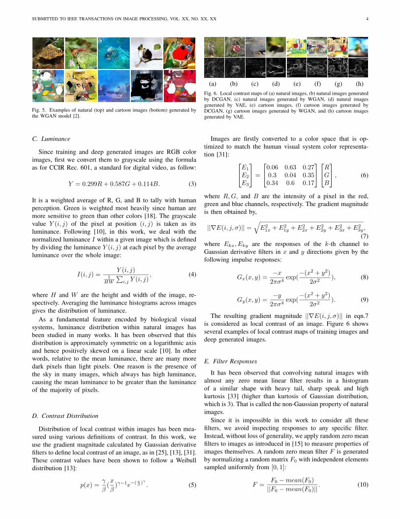
Fig. 5. Examples of natural (top) and cartoon images (bottom) generated bythe WGAN model [2].
C. Luminance
Since training and deep generated images are RGB colorimages, first we convert them to grayscale using the formulaas for CCIR Rec. 601, a standard for digital video, as follow:
Y = 0.299R+ 0.587G+ 0.114B. (3)
It is a weighted average of R, G, and B to tally with humanperception. Green is weighted most heavily since human aremore sensitive to green than other colors [18]. The grayscalevalue Y (i, j) of the pixel at position (i, j) is taken as itsluminance. Following [10], in this work, we deal with thenormalized luminance I within a given image which is definedby dividing the luminance Y (i, j) at each pixel by the averageluminance over the whole image:
I(i, j) =Y (i, j)
1HW
∑i,j Y (i, j)
, (4)
where H and W are the height and width of the image, re-spectively. Averaging the luminance histograms across imagesgives the distribution of luminance.
As a fundamental feature encoded by biological visualsystems, luminance distribution within natural images hasbeen studied in many works. It has been observed that thisdistribution is approximately symmetric on a logarithmic axisand hence positively skewed on a linear scale [10]. In otherwords, relative to the mean luminance, there are many moredark pixels than light pixels. One reason is the presence ofthe sky in many images, which always has high luminance,causing the mean luminance to be greater than the luminanceof the majority of pixels.
D. Contrast Distribution
Distribution of local contrast within images has been mea-sured using various definitions of contrast. In this work, weuse the gradient magnitude calculated by Gaussian derivativefilters to define local contrast of an image, as in [25], [13], [31].These contrast values have been shown to follow a Weibulldistribution [13]:
p(x) =γ
β(x
β)γ−1e−( xβ )
γ
. (5)
(a) (b) (c) (d) (e) (f) (g) (h)Fig. 6. Local contrast maps of (a) natural images, (b) natural images generatedby DCGAN, (c) natural images generated by WGAN, (d) natural imagesgenerated by VAE, (e) cartoon images, (f) cartoon images generated byDCGAN, (g) cartoon images generated by WGAN, and (h) cartoon imagesgenerated by VAE.
Images are firstly converted to a color space that is op-timized to match the human visual system color representa-tion [31]: E1
E2
E3
=
0.06 0.63 0.270.3 0.04 0.350.34 0.6 0.17
RGB
, (6)
where R,G, and B are the intensity of a pixel in the red,green and blue channels, respectively. The gradient magnitudeis then obtained by,
||∇E(i, j, σ)|| =√E2
1x + E21y + E2
2x + E22y + E2
3x + E23y,
(7)where Ekx, Eky are the responses of the k-th channel toGaussian derivative filters in x and y directions given by thefollowing impulse responses:
Gx(x, y) =−x2πσ4
exp(−(x2 + y2)
2σ2), (8)
Gy(x, y) =−y2πσ4
exp(−(x2 + y2)
2σ2). (9)
The resulting gradient magnitude ||∇E(i, j, σ)|| in eqn.7is considered as local contrast of an image. Figure 6 showsseveral examples of local contrast maps of training images anddeep generated images.
E. Filter Responses
It has been observed that convolving natural images withalmost any zero mean linear filter results in a histogramof a similar shape with heavy tail, sharp speak and highkurtosis [33] (higher than kurtosis of Gaussian distribution,which is 3). That is called the non-Gaussian property of naturalimages.
Since it is impossible in this work to consider all thesefilters, we avoid inspecting responses to any specific filter.Instead, without loss of generality, we apply random zero meanfilters to images as introduced in [15] to measure properties ofimages themselves. A random zero mean filter F is generatedby normalizing a random matrix F0 with independent elementssampled uniformly from [0, 1]:
F =F0 −mean(F0)
||F0 −mean(F0)||. (10)

SUBMITTED TO IEEE TRANSACTIONS ON IMAGE PROCESSING, VOL. XX, NO. XX, XX 5
Fig. 7. An example image and its four homogeneous regions.
F. Homogeneous Regions
Homogeneous regions in an image are the connected com-ponents where contrast does not exceed a certain threshold.Consider an image I of size H ×W and G gray levels. Wegenerate a series of thresholds t1, ..., tN , in which tn is theleast integer such that more than nHWN pixels have a grayvalue less than tn. Using these thresholds to segment an imageresults in N homogeneous regions. Figure 7 illustrates anexample image and its homogeneous regions.
Alvarez et al. [1] show that the number of homogeneousregions in natural images, denoted as N(s), as a function oftheir size s, obeys the following law:
N(s) = Ksc, (11)
where K is an image dependent constant, s denotes the area,and c is close to -2. Suppose image I1 is scaled into I2, suchthat I1(ax) = I2(x), a > 0. Let N1(s) = K1s
c denote thenumber of homogeneous regions of area s in I1. Then, forI2, we have N2(s) = N1(as) = K2s
c, so the number ofhomogeneous regions in natural images is a scale-invariantstatistic.
G. Power Spectrum
We adopt the most commonly used definition of powerspectrum in image statistics literature: “the power of differentfrequency components”. Formally, the power spectrum of animage is defined as the square of the magnitude of the imageFFT. Prior studies [7], [3], [9] have shown that the meanpower spectrum of natural images denoted as S(f), wheref is frequency, is scale invariant. It has the form of:
S(f) = Af−α, α ≈ 2. (12)
IV. EXPERIMENTS AND RESULTS
In this section, we report the experimental results of lu-minance distribution, contrast distribution, random filter re-sponse, distribution of homogeneous regions, and the meanpower spectrum of the training images and deep generatedimages. We use Welch’s t-test to test whether the statistics aresignificantly different between generated images and trainingimages (ImageNet-1 and Cartoon-1 in the tables). The largerp-value is, the more similar the generated images to trainingimages. Therefore, the models can be ranked according to t-test results. To make sure that our results are not specific to thechoice of training images, we sampled another set of trainingimages (ImageNet-2 and Cartoon-2 in the tables), and use t-test to measure difference between the two sets of trainingimages. All experiments are performed using Python 2.7 andOpenCV 2.0 on a PC with Intel i7 CPU and 32GB RAM. The
deep generative models used in this work are implemented inPyTorch1.
A. Luminance
Luminance distributions of training images and deep gener-ated images are shown in Figure 8. Average skewness valuesare shown in Table I.
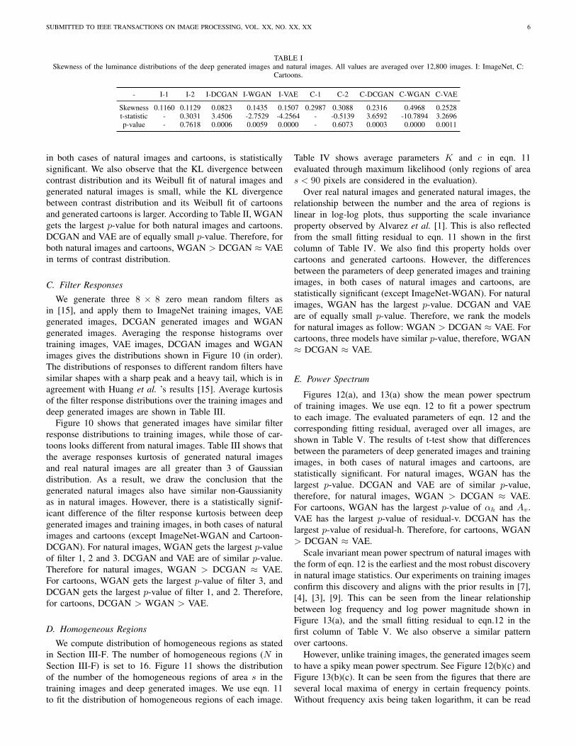
Results in in Figure 8 show that luminance distributions oftraining and generated images have similar shapes, while thoseof cartoons are markedly different from natural images. Fromin Table I, we can see that the luminance distributions overnatural images, cartoons, generated natural images and gener-ated cartoons all have positive skewness values. However, thedifference of skewness values between training and generatedimages is statistically significant (over both natural images andcartoons). The difference between skewness values over eachimage type (i.e., ImageNet-1 vs. ImageNet-2 or Cartoon-1 vs.Cartoon-2) is not significant, indicating that our our findingsare general and image sets are good representatives of thenatural or synthetic scenes. According to Table I, we rankthe models in terms of luminance distribution as follows. Fornatural images, WGAN > DCGAN > VAE, and for cartoons,VAE > DCGAN > WGAN.
(a) (b)Fig. 8. Luminance distribution. The distributions are all averaged over 12,800images. (a) natural images and generated natural images, (b) cartoons andgenerated cartoon images.
B. Contrast
It has been reported that the contrast distribution in naturalimages follows a Weibull distribution [12]. To test this on ourdata, first we fit a Weibull distribution (eqn. 5) to the histogramof each of the generated images and training images. Then,we use KL divergence to examine if the contrast distributionin deep generated images can be well modeled by a Weibulldistribution as in the case of natural images. If this is true, thefitted distributions will be close to the histogram as in trainingimages, and thus the KL divergence will be small.
Figure 9 shows that contrast distributions of training andgenerated images have similar shapes, while those of cartoonsare markedly different from natural images. Parameters ofthe fitted Weibull distribution and its KL divergence to thehistogram, as well as the corresponding t-test results are shownin Table II. We find that the contrast distributions in generatednatural images are also Weibull distributions. However, the dif-ference of parameters between training and generated images,
1https://github.com/pytorch
SUBMITTED TO IEEE TRANSACTIONS ON IMAGE PROCESSING, VOL. XX, NO. XX, XX 6
TABLE ISkewness of the luminance distributions of the deep generated images and natural images. All values are averaged over 12,800 images. I: ImageNet, C:
Cartoons.
- I-1 I-2 I-DCGAN I-WGAN I-VAE C-1 C-2 C-DCGAN C-WGAN C-VAE
Skewness 0.1160 0.1129 0.0823 0.1435 0.1507 0.2987 0.3088 0.2316 0.4968 0.2528t-statistic - 0.3031 3.4506 -2.7529 -4.2564 - -0.5139 3.6592 -10.7894 3.2696p-value - 0.7618 0.0006 0.0059 0.0000 - 0.6073 0.0003 0.0000 0.0011
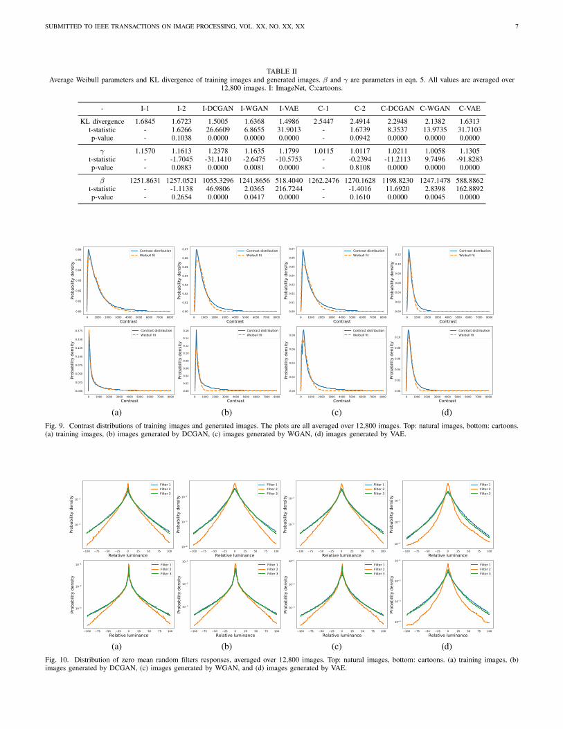
in both cases of natural images and cartoons, is statisticallysignificant. We also observe that the KL divergence betweencontrast distribution and its Weibull fit of natural images andgenerated natural images is small, while the KL divergencebetween contrast distribution and its Weibull fit of cartoonsand generated cartoons is larger. According to Table II, WGANgets the largest p-value for both natural images and cartoons.DCGAN and VAE are of equally small p-value. Therefore, forboth natural images and cartoons, WGAN > DCGAN ≈ VAEin terms of contrast distribution.
C. Filter Responses
We generate three 8 × 8 zero mean random filters asin [15], and apply them to ImageNet training images, VAEgenerated images, DCGAN generated images and WGANgenerated images. Averaging the response histograms overtraining images, VAE images, DCGAN images and WGANimages gives the distributions shown in Figure 10 (in order).The distributions of responses to different random filters havesimilar shapes with a sharp peak and a heavy tail, which is inagreement with Huang et al. ’s results [15]. Average kurtosisof the filter response distributions over the training images anddeep generated images are shown in Table III.
Figure 10 shows that generated images have similar filterresponse distributions to training images, while those of car-toons looks different from natural images. Table III shows thatthe average responses kurtosis of generated natural imagesand real natural images are all greater than 3 of Gaussiandistribution. As a result, we draw the conclusion that thegenerated natural images also have similar non-Gaussianityas in natural images. However, there is a statistically signif-icant difference of the filter response kurtosis between deepgenerated images and training images, in both cases of naturalimages and cartoons (except ImageNet-WGAN and Cartoon-DCGAN). For natural images, WGAN gets the largest p-valueof filter 1, 2 and 3. DCGAN and VAE are of similar p-value.Therefore for natural images, WGAN > DCGAN ≈ VAE.For cartoons, WGAN gets the largest p-value of filter 3, andDCGAN gets the largest p-value of filter 1, and 2. Therefore,for cartoons, DCGAN > WGAN > VAE.
D. Homogeneous Regions
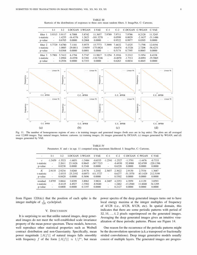
We compute distribution of homogeneous regions as statedin Section III-F. The number of homogeneous regions (N inSection III-F) is set to 16. Figure 11 shows the distributionof the number of the homogeneous regions of area s in thetraining images and deep generated images. We use eqn. 11to fit the distribution of homogeneous regions of each image.
Table IV shows average parameters K and c in eqn. 11evaluated through maximum likelihood (only regions of areas < 90 pixels are considered in the evaluation).
Over real natural images and generated natural images, therelationship between the number and the area of regions islinear in log-log plots, thus supporting the scale invarianceproperty observed by Alvarez et al. [1]. This is also reflectedfrom the small fitting residual to eqn. 11 shown in the firstcolumn of Table IV. We also find this property holds overcartoons and generated cartoons. However, the differencesbetween the parameters of deep generated images and trainingimages, in both cases of natural images and cartoons, arestatistically significant (except ImageNet-WGAN). For naturalimages, WGAN has the largest p-value. DCGAN and VAEare of equally small p-value. Therefore, we rank the modelsfor natural images as follow: WGAN > DCGAN ≈ VAE. Forcartoons, three models have similar p-value, therefore, WGAN≈ DCGAN ≈ VAE.
E. Power Spectrum
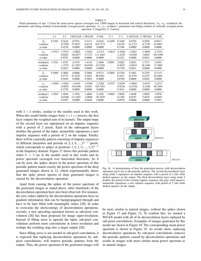
Figures 12(a), and 13(a) show the mean power spectrumof training images. We use eqn. 12 to fit a power spectrumto each image. The evaluated parameters of eqn. 12 and thecorresponding fitting residual, averaged over all images, areshown in Table V. The results of t-test show that differencesbetween the parameters of deep generated images and trainingimages, in both cases of natural images and cartoons, arestatistically significant. For natural images, WGAN has thelargest p-value. DCGAN and VAE are of similar p-value,therefore, for natural images, WGAN > DCGAN ≈ VAE.For cartoons, WGAN has the largest p-value of αh and Av .VAE has the largest p-value of residual-v. DCGAN has thelargest p-value of residual-h. Therefore, for cartoons, WGAN> DCGAN ≈ VAE.
Scale invariant mean power spectrum of natural images withthe form of eqn. 12 is the earliest and the most robust discoveryin natural image statistics. Our experiments on training imagesconfirm this discovery and aligns with the prior results in [7],[4], [3], [9]. This can be seen from the linear relationshipbetween log frequency and log power magnitude shown inFigure 13(a), and the small fitting residual to eqn.12 in thefirst column of Table V. We also observe a similar patternover cartoons.
However, unlike training images, the generated images seemto have a spiky mean power spectrum. See Figure 12(b)(c) andFigure 13(b)(c). It can be seen from the figures that there areseveral local maxima of energy in certain frequency points.Without frequency axis being taken logarithm, it can be read
SUBMITTED TO IEEE TRANSACTIONS ON IMAGE PROCESSING, VOL. XX, NO. XX, XX 7
TABLE IIAverage Weibull parameters and KL divergence of training images and generated images. β and γ are parameters in eqn. 5. All values are averaged over
12,800 images. I: ImageNet, C:cartoons.
- I-1 I-2 I-DCGAN I-WGAN I-VAE C-1 C-2 C-DCGAN C-WGAN C-VAE
KL divergence 1.6845 1.6723 1.5005 1.6368 1.4986 2.5447 2.4914 2.2948 2.1382 1.6313t-statistic - 1.6266 26.6609 6.8655 31.9013 - 1.6739 8.3537 13.9735 31.7103p-value - 0.1038 0.0000 0.0000 0.0000 - 0.0942 0.0000 0.0000 0.0000
γ 1.1570 1.1613 1.2378 1.1635 1.1799 1.0115 1.0117 1.0211 1.0058 1.1305t-statistic - -1.7045 -31.1410 -2.6475 -10.5753 - -0.2394 -11.2113 9.7496 -91.8283p-value - 0.0883 0.0000 0.0081 0.0000 - 0.8108 0.0000 0.0000 0.0000
β 1251.8631 1257.0521 1055.3296 1241.8656 518.4040 1262.2476 1270.1628 1198.8230 1247.1478 588.8862t-statistic - -1.1138 46.9806 2.0365 216.7244 - -1.4016 11.6920 2.8398 162.8892p-value - 0.2654 0.0000 0.0417 0.0000 - 0.1610 0.0000 0.0045 0.0000
(a) (b) (c) (d)Fig. 9. Contrast distributions of training images and generated images. The plots are all averaged over 12,800 images. Top: natural images, bottom: cartoons.(a) training images, (b) images generated by DCGAN, (c) images generated by WGAN, (d) images generated by VAE.
(a) (b) (c) (d)Fig. 10. Distribution of zero mean random filters responses, averaged over 12,800 images. Top: natural images, bottom: cartoons. (a) training images, (b)images generated by DCGAN, (c) images generated by WGAN, and (d) images generated by VAE.
SUBMITTED TO IEEE TRANSACTIONS ON IMAGE PROCESSING, VOL. XX, NO. XX, XX 8
TABLE IIIKurtosis of the distributions of responses to three zero mean random filters. I: ImageNet, C: Cartoons.
- I-1 I-2 I-DCGAN I-WGAN I-VAE C-1 C-2 C-DCGAN C-WGAN C-VAE
filter 1 5.9315 5.9117 6.7088 5.8742 11.3657 7.9789 7.9711 7.9786 8.2128 11.3245t-statistic - 1.4255 -16.4376 1.2623 -101.3270 - 0.0599 0.0029 -2.1637 -31.1486p-value - 0.6705 0.0000 0.2068 0.0000 - 0.9522 0.9977 0.0305 0.0000
filter 2 5.7729 5.6780 7.1181 5.9575 15.7773 7.3999 7.4632 7.4325 7.1798 12.0194t-statistic - 1.0885 -29.0011 -3.9459 -175.0824 - -0.6474 -0.3326 2.7206 -56.4231p-value - 0.0368 0.0000 0.0001 0.0000 - 0.5174 0.7395 0.0065 0.0000
filter 3 5.7901 5.7412 6.1794 5.7747 11.9817 5.1254 5.1916 5.3312 5.1954 8.4338t-statistic - 1.0504 -8.4558 0.3381 -110.7246 - -0.4870 -1.7311 -0.6991 -35.5865p-value - 0.2936 0.0000 0.7353 0.0000 - 0.6263 0.0834 0.4845 0.0000
(a) (b) (c) (d)Fig. 11. The number of homogeneous regions of area s in training images and generated images (both axes are in log units). The plots are all averagedover 12,800 images. Top: natural images, bottom: cartoons. (a) training images, (b) images generated by DCGAN, (c) images generated by WGAN, and (d)images generated by VAE.
TABLE IVParameters K and c in eqn. 11 computed using maximum likelihood. I: ImageNet, C: Cartoons.
- I-1 I-2 I-DCGAN I-WGAN I-VAE C-1 C-2 C-DCGAN C-WGAN C-VAE
c -1.5459 -1.5521 -1.6051 -1.5484 -0.6535 -1.2541 -1.2527 -1.3791 -1.4476 -0.7333t-statistic - 2.2611 23.1626 0.9645 -387.7215 - -0.4930 52.8988 82.6709 -220.1396p-value - 0.0238 0.0000 0.3348 0.0000 - 0.6220 0.0000 0.0000 0.0000
K 2.9135 2.9234 3.0268 2.9176 1.2102 2.3657 2.3622 2.9130 2.7534 1.3687t-statistic - -2.0333 -25.2192 -0.8973 411.3727 - 0.6277 -51.3570 -83.1429 212.5199p-value - 0.0420 0.0000 0.3696 0.0000 - 0.5302 0.0000 0.0000 0.0000
residual 3.8795 3.8844 3.8299 3.8962 3.9824 4.2407 4.2253 4.3959 4.1129 3.8593t-statistic - -0.4125 4.4927 -1.5561 -8.9440 - 1.2462 -13.2940 11.6040 34.1295p-value - 0.6800 0.0000 0.1197 0.0000 - 0.2127 0.0000 0.0000 0.0000
from Figure 12(b)(c) that the position of each spike is theinteger multiple of 4
128 cycle/pixel.
V. DISCUSSION
It is surprising to see that unlike natural images, deep gener-ated images do not meet the well-established scale invarianceproperty of the mean power spectrum. These models, however,well reproduce other statistical properties such as Weibullcontract distribution and non-Gaussianity. Specifically, meanpower magnitude ||A(f)|| of natural images falls smoothlywith frequency f of the form ||A(f)|| ∝ 1/fα, but mean
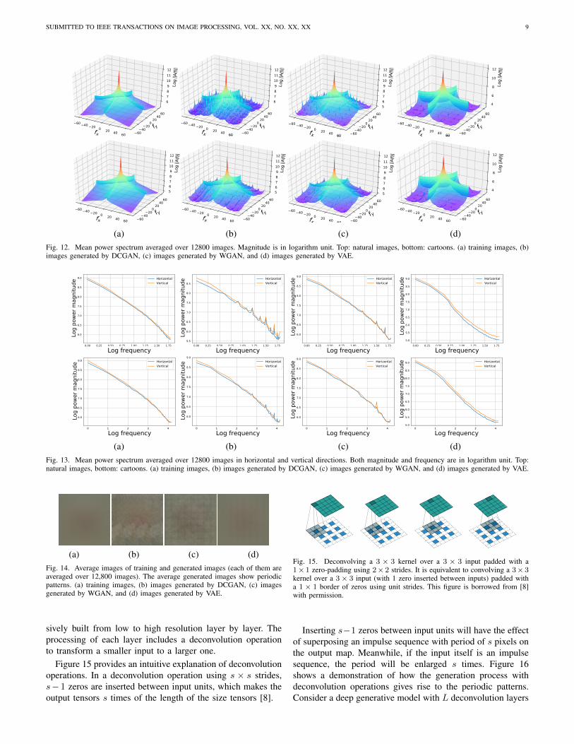
power spectra of the deep generated images turns out to havelocal energy maxima at the integer multiples of frequencyof 4/128 (i.e., 4/128, 8/128, etc). In spatial domain, thisindicates that there are some periodic patterns with period of32, 16, ..., 4, 2 pixels superimposed on the generated images.Averaging the deep generated images gives an intuitive visu-alization of these periodic patterns. Please see Figure 14.
One reason for the occurrence of the periodic patterns mightbe the deconvolution operation (a.k.a transposed or fractionallystrided convolutions). Deep image generative models usuallyconsist of multiple layers. The generated images are progres-
SUBMITTED TO IEEE TRANSACTIONS ON IMAGE PROCESSING, VOL. XX, NO. XX, XX 9
Log
||A(f)
||
Log
||A(f)
||
Log
||A(f)
||
Log
||A(f)
||
Log
||A(f)
||
Log
||A(f)
||
Log
||A(f)
||
Log
||A(f)
||
(a) (b) (c) (d)Fig. 12. Mean power spectrum averaged over 12800 images. Magnitude is in logarithm unit. Top: natural images, bottom: cartoons. (a) training images, (b)images generated by DCGAN, (c) images generated by WGAN, and (d) images generated by VAE.
(a) (b) (c) (d)Fig. 13. Mean power spectrum averaged over 12800 images in horizontal and vertical directions. Both magnitude and frequency are in logarithm unit. Top:natural images, bottom: cartoons. (a) training images, (b) images generated by DCGAN, (c) images generated by WGAN, and (d) images generated by VAE.
(a) (b) (c) (d)Fig. 14. Average images of training and generated images (each of them areaveraged over 12,800 images). The average generated images show periodicpatterns. (a) training images, (b) images generated by DCGAN, (c) imagesgenerated by WGAN, and (d) images generated by VAE.
sively built from low to high resolution layer by layer. Theprocessing of each layer includes a deconvolution operationto transform a smaller input to a larger one.
Figure 15 provides an intuitive explanation of deconvolutionoperations. In a deconvolution operation using s × s strides,s− 1 zeros are inserted between input units, which makes theoutput tensors s times of the length of the size tensors [8].
Figure 4.4: The transpose of convolving a 3 ⇥ 3 kernel over a 5 ⇥ 5 input usingfull padding and unit strides (i.e., i = 5, k = 3, s = 1 and p = 2). It is equivalentto convolving a 3 ⇥ 3 kernel over a 7 ⇥ 7 input using unit strides (i.e., i0 = 7,k0 = k, s0 = 1 and p0 = 0).
Figure 4.5: The transpose of convolving a 3 ⇥ 3 kernel over a 5 ⇥ 5 input using2 ⇥ 2 strides (i.e., i = 5, k = 3, s = 2 and p = 0). It is equivalent to convolvinga 3 ⇥ 3 kernel over a 2 ⇥ 2 input (with 1 zero inserted between inputs) paddedwith a 2 ⇥ 2 border of zeros using unit strides (i.e., i0 = 2, i0 = 3, k0 = k, s0 = 1and p0 = 2).
Figure 4.6: The transpose of convolving a 3⇥3 kernel over a 5⇥5 input paddedwith a 1 ⇥ 1 border of zeros using 2 ⇥ 2 strides (i.e., i = 5, k = 3, s = 2 andp = 1). It is equivalent to convolving a 3 ⇥ 3 kernel over a 2 ⇥ 2 input (with1 zero inserted between inputs) padded with a 1 ⇥ 1 border of zeros using unitstrides (i.e., i0 = 3, i0 = 5, k0 = k, s0 = 1 and p0 = 1).
24
Fig. 15. Deconvolving a 3 × 3 kernel over a 3 × 3 input padded with a1× 1 zero-padding using 2× 2 strides. It is equivalent to convolving a 3× 3kernel over a 3× 3 input (with 1 zero inserted between inputs) padded witha 1 × 1 border of zeros using unit strides. This figure is borrowed from [8]with permission.
Inserting s−1 zeros between input units will have the effectof superposing an impulse sequence with period of s pixels onthe output map. Meanwhile, if the input itself is an impulsesequence, the period will be enlarged s times. Figure 16shows a demonstration of how the generation process withdeconvolution operations gives rise to the periodic patterns.Consider a deep generative model with L deconvolution layers
SUBMITTED TO IEEE TRANSACTIONS ON IMAGE PROCESSING, VOL. XX, NO. XX, XX 10
TABLE VFitted parameters of eqn. 12 from the mean power spectra (averaged over 12800 images in horizontal and vertical directions). Ah, αh, residual-h: the
parameters and fitting residual of horizontally averaged power spectrum; Av , αv , residual-v: parameters and fitting residual of vertically averaged powerspectrum. I: ImageNet, C: Cartoon.
- I-1 I-2 I-DCGAN I-WGAN I-VAE C-1 C-2 C-DCGAN C-WGAN C-VAE
Ah 9.2383 9.2418 8.9781 9.2113 8.8342 9.1690 9.1649 9.0792 9.2039 8.9417t-statistic - -0.7504 57.9637 6.0118 105.7172 - 0.6150 14.1713 -6.1758 43.9667p-value - 0.4530 0.0000 0.0000 0.0000 - 0.5386 0.0000 0.0000 0.0000
αh -1.9733 -1.9733 -1.8882 -1.9542 -2.3313 -1.9813 -1.9768 -1.9461 -1.9869 -2.3234t-statistic - 0.0262 -26.6477 -5.7127 111.1663 - -1.2210 -9.8188 1.6845 102.4380p-value - 0.9791 0.0000 0.0000 0.0000 - 0.2221 0.0000 0.0921 0.0000
residual-h 1.5341 1.5523 2.5745 1.4119 2.1860 2.0091 2.0202 2.0621 1.7371 1.8183t-statistic - -1.2755 -61.2857 10.6709 -52.3226 - -0.5625 -2.9619 18.1469 12.7869p-value - 0.2021 0.0000 0.0000 0.0000 - 0.5738 0.0031 0.0000 0.0000
Av 9.2909 9.2884 9.0066 9.2886 8.9713 9.2804 9.2794 9.1861 9.2792 9.1315t-statistic - 0.5775 67.4247 0.5441 86.9562 - 0.1637 16.2791 0.2273 29.4495p-value - 0.5636 0.0000 0.5864 0.0000 - 0.8700 0.0000 0.8202 0.0000
αv -1.9592 -1.9562 -1.8165 -1.9748 -2.3382 -2.0327 -2.0295 -1.9845 -2.0197 -2.4213t-statistic - -0.8855 -45.6106 5.0362 105.7561 - -0.9126 -14.5242 -4.2188 96.7694p-value - 0.3759 0.0000 0.0000 0.0000 - 0.3615 0.0000 0.0000 0.0000
residual-v 1.4563 1.4656 1.7456 1.4804 2.1362 1.9864 1.9836 1.8448 1.8995 1.9976t-statistic - -0.6300 -21.2443 -2.0089 -49.1039 - 0.1285 8.0197 5.4635 -0.6603p-value - 0.5287 0.0000 0.0446 0.0000 - 0.8978 0.0000 0.0000 0.5091
with 2 × 2 strides, similar to the models used in this work.When this model builds images from 1×1×c tensors, the firstlayer outputs the weighted sum of its kernels. The output mapsof the second layer are superposed on an impulse sequencewith a period of 2 pixels. Each of the subsequent layersdoubles the period of the input, meanwhile superposes a newimpulse sequence with a period of 2 on the output. Finally,there will be a periodic pattern consisting of impulse sequencesof different intensities and periods of 2, 4, 8, ..., 2L−1 pixels,which corresponds to spikes at positions 1/2, 1/4, ..., 1/2L−1
in the frequency domain. Figure 17 shows this periodic patternwhen L = 5 (as in the models used in this work) and itspower spectrum (averaged over horizontal direction). As itcan be seen, the spikes shown in the power spectrum of thisperiodic pattern match exactly the power spectrum of the deepgenerated images shown in 12, which experimentally showsthat the spiky power spectra of deep generated images iscaused by the deconvolution operation.
Apart from causing the spikes of the power spectrum ofthe generated images as stated above, other drawbacks of thedeconvolution operation have also been observed. For instance,the zero values added by the deconvolution operations have nogradient information that can be backpropagated through andhave to be later filled with meaningful values [28]. In orderto overcome the shortcomings of deconvolution operations,recently, a new upscaling operation known as sub-pixel con-volution [26] has been proposed for image super-resolution.Instead of filling zeros to upscale the input, sub-pixel con-volutions perform more convolutions in lower resolution andreshape the resulting map into a larger output [28].
Since filling zeros is not needed in sub-pixel convolution, itis expected that replacing deconvolution operations by sub-pixel convolutions, will remove periodic patterns from theoutput. Thus, the power spectrum of the generated images will
deconv
conv
conv
deconv
deconv
Fig. 16. A demonstration of how the generation process with deconvolutionoperations gives rise to the periodic patterns. The second deconvolution layerusing stride 2 superposes an impulse sequence with a period of 2 (the whitedashed squares) on the output. The third deconvolution layer using stride 2doubles the period of the existing impulse sequence (the gray solid squares),meanwhile superposes a new impulse sequence with period of 2 (the whitedashed squares) on the output.
be more similar to natural images, without the spikes shownin Figure 17 and Figure 12. To confirm this, we trained aWGAN model with all of its deconvolution layers replaced bysub-pixel convolutions. Examples of images generated by thismodel are shown in Figure 18. The corresponding mean powerspectrum is shown in Figure 19. As results show, replacingdeconvolution operations by sub-pixel convolutions removesthe periodic patterns caused by deconvolution operations andresults in images with more similar mean power spectrum asin natural images.

SUBMITTED TO IEEE TRANSACTIONS ON IMAGE PROCESSING, VOL. XX, NO. XX, XX 11
(a) (c)Fig. 17. (a) a periodic pattern consisting of impulse sequences of differentintensities and periods of 2, 4, 8, ..., 2L−1 pixels, where L is the numberof layers, and L = 5 in this case. (b) the power spectrum of this pattern(averaged over horizontal direction) matches exactly the power spectrum ofthe deep generated images shown in 12, which experimentally shows that thespiky power spectra of deep generated images is caused by the deconvolutionoperation.
Fig. 18. Examples of images generated by WGAN with all deconvolutionlayers replaced by sub-pixel convolutions.
VI. SUMMARY AND CONCLUSION
We explore statistics of images generated by state-of-the-art deep generative models (VAE, DCGAN and WGAN) andcartoon images with respect to the natural image statistics.Our analyses on training natural images corroborates existingfindings of scale invariance, non-Gaussianity, and Weibull con-trast distribution on natural image statistics. We also find non-Gaussianity and Weibull contrast distribution for generatedimages with VAE, DCGAN and WGAN. These statistics,however, are still significantly different. Unlike natural images,neither of the generated images has scale invariant mean powerspectrum magnitude, which indicates extra structures in thegenerated images. We show that these extra structures arecaused by the deconvolution operations. Replacing decon-volution layers in the deep generative models by sub-pixelconvolution helps them generate images with mean powerspectrum closer to the mean power spectrum of natural images.
Inspecting how well the statistics of the generated imagesmatch natural scenes, can a) reveal the degree to which deeplearning models capture the essence of the natural scenes, b)provide a new dimension to evaluate models, and c) suggestpossible directions to improve image generation models. Cor-respondingly, two possible future works include:
1) Building a new metric for evaluating deep image gener-ative models based on image statistics, and
2) Designing deep image generative models that bettercapture statistics of the natural scenes (e.g., through
designing new loss functions).To encourage future explorations in this area and assess the
quality of images by other image generation models, we shareour cartoon dataset and code for computing the statistics ofimages at: https://github.com/zengxianyu/generate.
ACKNOWLEDGMENT
The authors would like to thank several teachers at DUTfor their helpful comments on an earlier version of this work.We wish to thank Mr. Yingming Wang for providing somecartoon videos, and Dr. Lijun Wang for his help.
REFERENCES
[1] L. Alvarez, Y. Gousseau, and J.-M. Morel. The size of objects innatural and artificial images. Advances in Imaging and Electron Physics,111:167–242, 1999.
[2] M. Arjovsky, S. Chintala, and L. Bottou. Wasserstein gan. arXiv preprintarXiv:1701.07875, 2017.
[3] G. Burton and I. R. Moorhead. Color and spatial structure in naturalscenes. Applied Optics, 26(1):157–170, 1987.
[4] R. W. Cohen, I. Gorog, and C. R. Carlson. Image descriptors fordisplays. Technical report, DTIC Document, 1975.
[5] J. Deng, W. Dong, R. Socher, L.-J. Li, K. Li, and L. Fei-Fei. Imagenet: Alarge-scale hierarchical image database. In Computer Vision and PatternRecognition, 2009. CVPR 2009. IEEE Conference on, pages 248–255.IEEE, 2009.
[6] E. L. Denton, S. Chintala, R. Fergus, et al. Deep generative imagemodels using a laplacian pyramid of adversarial networks. In Advancesin neural information processing systems, pages 1486–1494, 2015.
[7] N. Deriugin. The power spectrum and the correlation function of thetelevision signal. Telecommunications, 1(7):1–12, 1956.
[8] V. Dumoulin and F. Visin. A guide to convolution arithmetic for deeplearning. arXiv preprint arXiv:1603.07285, 2016.
[9] D. J. Field. Relations between the statistics of natural images and theresponse properties of cortical cells. JOSA A, 4(12):2379–2394, 1987.
[10] W. S. Geisler. Visual perception and the statistical properties of naturalscenes. Annu. Rev. Psychol., 59:167–192, 2008.
[11] D. Geman and A. Koloydenko. Invariant statistics and coding of naturalmicroimages. In IEEE Workshop on Statistical and ComputationalTheories of Vision, 1999.
[12] J.-M. Geusebroek and A. W. Smeulders. A six-stimulus theory forstochastic texture. International Journal of Computer Vision, 62(1-2):7–16, 2005.
[13] S. Ghebreab, S. Scholte, V. Lamme, and A. Smeulders. A biologicallyplausible model for rapid natural scene identification. In Advances inNeural Information Processing Systems, pages 629–637, 2009.
[14] I. Goodfellow, J. Pouget-Abadie, M. Mirza, B. Xu, D. Warde-Farley,S. Ozair, A. Courville, and Y. Bengio. Generative adversarial nets. InAdvances in neural information processing systems, pages 2672–2680,2014.
[15] J. Huang and D. Mumford. Statistics of natural images and models. InComputer Vision and Pattern Recognition, 1999. IEEE Computer SocietyConference On., volume 1, pages 541–547. IEEE, 1999.
[16] A. Hyvarinen, J. Hurri, and P. O. Hoyer. Natural Image Statistics:A Probabilistic Approach to Early Computational Vision., volume 39.Springer Science & Business Media, 2009.
[17] D. J. Im, C. D. Kim, H. Jiang, and R. Memisevic. Generating imageswith recurrent adversarial networks. arXiv preprint arXiv:1602.05110,2016.
[18] C. Kanan and G. W. Cottrell. Color-to-grayscale: does the method matterin image recognition? PloS one, 7(1):e29740, 2012.
[19] D. P. Kingma and M. Welling. Auto-encoding variational bayesge. arXivpreprint arXiv:1312.6114, 2013.
[20] A. Krizhevsky, I. Sutskever, and G. E. Hinton. Imagenet classificationwith deep convolutional neural networks. In Advances in neuralinformation processing systems, pages 1097–1105, 2012.
[21] A. B. Lee, D. Mumford, and J. Huang. Occlusion models for naturalimages: A statistical study of a scale-invariant dead leaves model.International Journal of Computer Vision, 41(1):35–59, 2001.
[22] D. Mumford and B. Gidas. Stochastic models for generic images.Quarterly of applied mathematics, 59(1):85–111, 2001.
[23] A. Radford, L. Metz, and S. Chintala. Unsupervised representationlearning with deep convolutional generative adversarial networks. arXivpreprint arXiv:1511.06434, 2015.
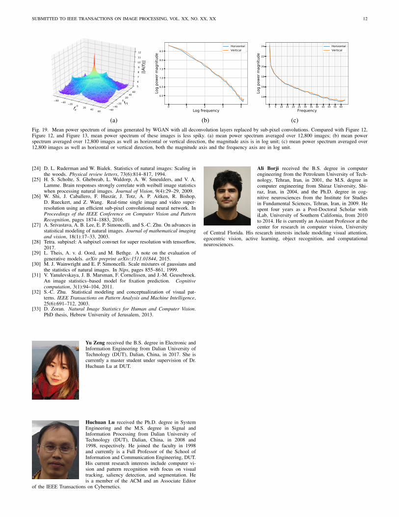
SUBMITTED TO IEEE TRANSACTIONS ON IMAGE PROCESSING, VOL. XX, NO. XX, XX 12
(a) (b) (c)Fig. 19. Mean power spectrum of images generated by WGAN with all deconvolution layers replaced by sub-pixel convolutions. Compared with Figure 12,Figure 12, and Figure 13, mean power spectrum of these images is less spiky. (a) mean power spectrum averaged over 12,800 images; (b) mean powerspectrum averaged over 12,800 images as well as horizontal or vertical direction, the magnitude axis is in log unit; (c) mean power spectrum averaged over12,800 images as well as horizontal or vertical direction, both the magnitude axis and the frequency axis are in log unit.
[24] D. L. Ruderman and W. Bialek. Statistics of natural images: Scaling inthe woods. Physical review letters, 73(6):814–817, 1994.
[25] H. S. Scholte, S. Ghebreab, L. Waldorp, A. W. Smeulders, and V. A.Lamme. Brain responses strongly correlate with weibull image statisticswhen processing natural images. Journal of Vision, 9(4):29–29, 2009.
[26] W. Shi, J. Caballero, F. Huszar, J. Totz, A. P. Aitken, R. Bishop,D. Rueckert, and Z. Wang. Real-time single image and video super-resolution using an efficient sub-pixel convolutional neural network. InProceedings of the IEEE Conference on Computer Vision and PatternRecognition, pages 1874–1883, 2016.
[27] A. Srivastava, A. B. Lee, E. P. Simoncelli, and S.-C. Zhu. On advances instatistical modeling of natural images. Journal of mathematical imagingand vision, 18(1):17–33, 2003.
[28] Tetra. subpixel: A subpixel convnet for super resolution with tensorflow,2017.
[29] L. Theis, A. v. d. Oord, and M. Bethge. A note on the evaluation ofgenerative models. arXiv preprint arXiv:1511.01844, 2015.
[30] M. J. Wainwright and E. P. Simoncelli. Scale mixtures of gaussians andthe statistics of natural images. In Nips, pages 855–861, 1999.
[31] V. Yanulevskaya, J. B. Marsman, F. Cornelissen, and J.-M. Geusebroek.An image statistics–based model for fixation prediction. Cognitivecomputation, 3(1):94–104, 2011.
[32] S.-C. Zhu. Statistical modeling and conceptualization of visual pat-terns. IEEE Transactions on Pattern Analysis and Machine Intelligence,25(6):691–712, 2003.
[33] D. Zoran. Natural Image Statistics for Human and Computer Vision.PhD thesis, Hebrew University of Jerusalem, 2013.
Yu Zeng received the B.S. degree in Electronic andInformation Engineering from Dalian University ofTechnology (DUT), Dalian, China, in 2017. She iscurrently a master student under supervision of Dr.Huchuan Lu at DUT.
Huchuan Lu received the Ph.D. degree in SystemEngineering and the M.S. degree in Signal andInformation Processing from Dalian University ofTechnology (DUT), Dalian, China, in 2008 and1998, respectively. He joined the faculty in 1998and currently is a Full Professor of the School ofInformation and Communication Engineering, DUT.His current research interests include computer vi-sion and pattern recognition with focus on visualtracking, saliency detection, and segmentation. Heis a member of the ACM and an Associate Editor
of the IEEE Transactions on Cybernetics.
Ali Borji received the B.S. degree in computerengineering from the Petroleum University of Tech-nology, Tehran, Iran, in 2001, the M.S. degree incomputer engineering from Shiraz University, Shi-raz, Iran, in 2004, and the Ph.D. degree in cog-nitive neurosciences from the Institute for Studiesin Fundamental Sciences, Tehran, Iran, in 2009. Hespent four years as a Post-Doctoral Scholar withiLab, University of Southern California, from 2010to 2014. He is currently an Assistant Professor at thecenter for research in computer vision, University
of Central Florida. His research interests include modeling visual attention,egocentric vision, active learning, object recognition, and computationalneurosciences.


![IEEE TRANSACTIONS ON WIRELESS COMMUNICATIONS, …IEEE TRANSACTIONS ON WIRELESS COMMUNICATIONS, VOL. XX, NO. XX, XXX 201X 2 processes before directional data communications [14]. To](https://img.pdfslide.us/doc/110x75/5f767a2b993c5b4ed7036e7f/ieee-transactions-on-wireless-communications-ieee-transactions-on-wireless-communications.jpg)