Subject BUSINESS ECONOMICS Paper No and Title 8

____________________________________________________________________________________________________

BUSINESS ECONOMICS

PAPER NO. : 8, FUNDAMENTALS OF ECONOMETRICS

MODULE NO. : 6, HYPOTHESIS TESTING: TEST OF SIGNIFICANCE APPROACH

Subject BUSINESS ECONOMICS

Paper No and Title 8 , Fundamentals of Econometrics

Module No and Title 6, Hypothesis Testing: Test of significance approach

Module Tag BSE_P8_M6

____________________________________________________________________________________________________

BUSINESS ECONOMICS



TABLE OF CONTENTS

1. Learning Outcomes

2. Introduction

3. What does this hypothesis mean and imply?

4. One sided tests

5. Summary

____________________________________________________________________________________________________

BUSINESS ECONOMICS



1. Learning Outcomes

After reading this module, the learning outcomes are such that the students will be able to:

Understand the properties of the hypothesis testing

Identify its implications

Assess the fitted econometric models

2. Introduction

Hypothesis Testing

Fitting the regression line is only the first and a very small step in econometric analysis. In

applied economics, we are generally interested in testing the hypothesis about some hypothesized

value of the population parameter. Let’s say we have a random sample 𝑥1, 𝑥2, … … , 𝑥𝑛 of a

random variable X with PDF 𝑓(𝑥; 𝜇 ). Regression analysis helps us to obtain the estimate of 𝜇,

say �̂�. Hypothesis testing implies deciding whether �̂� is compatible with some hypothesized

value𝜇0. To set up a hypothesis test, we formally state the hypothesis as:

𝐻0: 𝜇 = 𝜇0

𝐻1: 𝜇 ≠ 𝜇0

Where 𝐻0 is called the null hypothesis and 𝐻1 is called the alternate hypothesis.

3. What does this hypothesis mean and imply ?

Let us start with a random variable X i.e. 𝑋~𝑁(𝜇, 𝜎2). Suppose we define our null hypothesis to

be

𝐻0: 𝜇 = 𝜇0

𝐻1: 𝜇 ≠ 𝜇0

To proceed, first step is to draw a sample from X and calculate its mean, �̅�. Value of �̅� obtained

from repeated sample will be normally distributed with mean 𝜇0 and variance 𝜎2 𝑛⁄ . Null

hypothesis being true resonates with the above explanation. Such a distribution with the null

being true is shown below:

____________________________________________________________________________________________________

BUSINESS ECONOMICS



If �̂� is a good estimator of 𝜇, then it will take a value close to 𝜇 i.e. �̂�-𝜇 will be small. If the null

hypothesis is true, then �̂� − 𝜇0 = (�̂� − 𝜇)+ (𝜇 − 𝜇0) , should be small as �̂�-𝜇 is small and the

second term is zero. If the alternate hypothesis is true, then �̂� − 𝜇0 = (�̂� − 𝜇)+ (𝜇 − 𝜇0) should

be large as �̂�-𝜇and𝜇 − 𝜇0 ≠ 0. Small or large depends upon the distribution of the estimator.

In the model set above, we don’t expect �̅� to be exactly equal to 𝜇0. There is no reason to deny

the possibility but the chances are rare. If the mean is far off from𝜇0, there are two possibilities;

either reject the null or do not reject the null. Either way, the decision will contain some element

of error i.e. rejecting a true null hypothesis (Type 1) or accepting a false null hypothesis (Type 2).

There is no fool proof way of deciding.

If the probability of the mean, which lies far off from 𝜇0 , is less than the level of significance,

we can conclude to reject the null hypothesis. For e.g. if the probability is less than 5% i.e. lies in

the upper and lower 2.5% tails (as shown in the figure). Thus, the probability of the mean being

1.96 standard deviations away is 5%.

____________________________________________________________________________________________________

BUSINESS ECONOMICS



Figure 2: Decision Rule

Source: Dougherty

The figure suggests that the null would be rejected if �̅� lies in the shaded area i.e. if

�̅� > 𝜇𝑜 + 1.96 𝑠𝑡𝑑 𝑑𝑒𝑣(𝑋)̅̅ ̅ or,

�̅� < 𝜇𝑜 − 1.96 𝑠𝑡𝑑 𝑑𝑒𝑣(𝑋)̅̅ ̅

A simple rearrangement would lead us to,

�̅�−𝜇0

𝑠𝑑(�̅�)> 1.96 or,

�̅� − 𝜇0

𝑠𝑑(�̅�)< −1.96

Admittedly, we can term the LHS as z statistic. Therefore, we reject the null hypothesis when

|𝑧|>1.96.

As mentioned before, the decision rule established above is not flawless. Let us go back to our

initial condition of 𝐻𝑜 being true. There is 5% probability that �̅� will lie far away from 𝜇𝑜 in the

rejection region. It also means that there is 5% probability of a type 1 error i.e. probability of

____________________________________________________________________________________________________

BUSINESS ECONOMICS



rejecting a true null hypothesis is 5%1. The researcher has the liberty to settle the risk of type 1

error and accordingly look up the critical value.

To sum up, there are three possible outcomes:

• Correct decision

• Rejecting a true hypothesis– Type I error.

• Accepting a false hypothesis– Type II error.

To be able to perform the test, we need an additional knowledge of the sampling distributions of

the estimators. It will be impossible to perform hypothesis testing without this knowledge,

prerequisite of which is the assumption that the error term is normally distributed.

Given the following model,

𝑌𝑖 = 𝛼 + 𝛽𝑋𝑖 + 𝑈𝑖

It simply means that 𝑈𝑖 follows normal distribution with mean zero and variance 𝜎2 i.e. N (0,𝜎2).

The principle reason behind this assumption lies in the Central Limit Theorem (CLT)2.

Referring back to the basics, error term is defined as all those factors that affect Y but not

included in the model due to non-availability of data, omission etc. Supposing these factors are

random, then U represents the sum of random variables. Hence, by applying CLT we can,

undoubtedly, impose normality assumption on the error term. Thus, 𝑈~𝑁(0, 𝜎2).

From this, we derive the probability distributions of the estimators of𝛼 and𝛽. The estimators are

in fact linear functions of U3. Applying one of the properties of normal distribution that any linear

function of a normally distributed variable is also normally distributed, it can be deduced that,

�̂�~𝑁(𝛼, 𝜎�̂�2)

�̂�~𝑁(𝛽, 𝜎�̂�2)

With this background, we now set the foundation for hypothesis testing. Suppose we wish to test

something about 𝛽, as already mentioned, it follows normal distribution. By standardizing it , we

get,

𝑍 =�̂� − 𝛽

𝑠𝑒(𝛽)~𝑁(0,1)

Since 𝜎2 is not known, replacing the population estimator by its sample estimator, we get a new

variable,

1 Similar claim can be made for 1% level of significance. If a coefficient is significant at 1%, it will be significant at 5% as well. However, vice-versa may not be true. 2 Gujarati and Porter(2010) define CLT in the following way, “If there is a large number of independent and identically distributed random variables, then, with few exceptions, the distribution of their sum tends to be a normal distribution as the number of such variables increases indefinitely”. 3 See Know more section 1

____________________________________________________________________________________________________

BUSINESS ECONOMICS



�̂� − 𝛽

𝑠𝑒(𝛽)̂~𝑡𝑛−2

Hence, we use t distribution to test the null hypothesis4. The calculated t has different sampling

distribution under the null and under the alternate hypothesis, being higher under the latter. A

higher t would be consistent with the alternate hypothesis. Thus, a higher t would mean rejection

of the null hypothesis.

The following examples intend to illustrate the theory above.

Example 1: Suppose we have data on income and expenditure for 10 households.

Table 1: Income (𝒙𝒕) and Expenditure (𝒚𝒕)

�̂� = ∑(𝒙𝒕−�̅�)( 𝒚𝒕−�̅�)

∑(𝒙𝒕−�̅�)2 = 0.45;

�̂� = �̅� − �̂��̅� = 35.72

�̂�2 =∑ �̂�𝑡

2

𝑛−2= 98.98;

𝑣𝑎𝑟(�̂�) =�̂�2

∑(𝒙𝒕−�̅�)2=0.0030

4 Difference between �̂� and 𝛽 small implies t value to be small. If �̂� = 𝛽, t will be, zero implying null

hypothesis will not be rejected. Thus, as the difference between �̂� and 𝛽 increases, likelihood of rejecting the null hypothesis increases.

____________________________________________________________________________________________________

BUSINESS ECONOMICS



After running through the necessary calculations, the next is to test if income and expenditure are

related i.e. null hypothesis is as follows,

𝐻0: 𝛽 = 0

𝐻𝑎: 𝛽 ≠ 0

Test statistic, t = �̂�−𝛽

𝑠𝑒(𝛽)̂ =

�̂�−0

0.054 = 8.30

If the level of significance is 5%, next step is to look out for critical value at that level from the t

table i.e.

𝑡𝑐𝑟𝑖𝑡𝑖𝑐𝑎𝑙 𝑎𝑡 8 = 2.306. The absolute value of t exceeds the critical value, which implies that we

can reject the null hypothesis i.e. 𝛽 is significantly different from zero. In this case, the test is

statistically significant; hence, we can reject the null. It simply means that the probability of the

difference between �̂� and zero is due to mere chance is less than the level of significance and thus

can easily reject the null hypothesis. On contrary, if the test is statistically insignificant implies

that the probability of the difference between the estimator and the hypothesized value is more

than the level of significance, thus we cannot reject the null (Gujarati and Porter, 2010).

Let us look at another example5 where in hourly earnings is a function of years of schooling.

Example 2:

In a similar manner, let us test if the level of schooling affects earnings. Hence, the null

hypothesis is set as

𝐻0: 𝛽 = 0 𝐻𝑎: 𝛽 ≠ 0

5Example taken from Christopher Dougherty, Introduction to Econometrics, 4th Edition.

____________________________________________________________________________________________________

BUSINESS ECONOMICS



The intention is to reject the null hypothesis as only then a relation between earnings and

schooling can be established. T statistic can be easily calculated by looking at the regression

output6,

𝑡 =2.45

0.23 = 10.65

𝑡𝑐𝑎𝑙 > 𝑡𝑐𝑟𝑖𝑡𝑖𝑐𝑎𝑙(1.96)

The result decides in favour of rejecting the null hypothesis and concluding that earnings are

significantly affected by the level of schooling. The column next to t stat in the regression output

above is also a useful to test the significance of the coefficients. This P value or the probability

value is the exact probability of committing a Type 1 error, under the null. The level of

significance7 is the largest probability of making a Type 1 error. Whereas, p value is the smallest

probability, given t-statistic. If this p value happens to be smaller than the level of significance,

because the probability of making the type 1 error is very small, we can safely reject the null

hypothesis8. The method has an edge over the earlier as it allows us to know the exact probability

of making a type 1 error.

In our example, the p value for the schooling coefficient is 0 i.e. the exact probability of making a

type 1 error here is zero and thus the coefficient will be significant at all levels.

Example 3: Suppose in our example 1, we want to test whether marginal propensity to consume

is equal to 1. Accordingly, hypothesis is set as,

𝐻0: 𝛽 = 1

𝐻𝑎: 𝛽 < 1

𝑡 =�̂�−1

√𝑣𝑎𝑟(�̂�)

=0.455

√0.0030= -9.96

𝑡𝑐𝑟𝑖𝑡𝑖𝑐𝑎𝑙 𝑎𝑡 8 = −1.860

Thus, 𝑡𝑐𝑎𝑙 > 𝑡𝑐𝑟𝑖𝑡𝑖𝑐𝑎𝑙 , so we reject the null in favour of the alternate hypothesis.

4. One – sided tests

The above was an example of a one sided test. The decision to perform depends upon the

question that we wish to answer. We shall see that one sided tests reduce the risk of type 1 error.

One way of reducing the risk (in two-sided test) is to perform the test at 1% significance level a

6 Also can be directly seen from t stat column. 7 It is the area right to the critical value. 8 Please refer to the know more section 2 for further understanding of Type 1 and Type 2 errors.

____________________________________________________________________________________________________

BUSINESS ECONOMICS



an alternative to a 5%. The alternate hypothesis was set as 𝜇 ≠ 𝜇0 i.e. must be equal to some 𝜇1.

For simplicity, let 𝜇1 > 𝜇0.

Therefore,

𝐻0: 𝜇 = 𝜇0

𝐻1: 𝜇 = 𝜇1

At 5% level of significance, if �̅� lies in the upper or lower 2.5% tail, we reject the null. Given the

assumption, �̅� should lie in the upper tail. This would also be compatible with the alternate

hypothesis, if it is true. on the contrary, if it lies in the lower tail rejection region, the test would

suggest to reject the null, although probability of �̅� lying there should be zero (given the

assumption). Thus, in such a case it would be logical to accept the null i.e. reject 𝐻0 only when it

lies on the upper tail as shown in the figure 3 below:

We could also perform a 5% test by just increasing the rejection region to that extent. Note that

alternate could have another possibility where, 𝜇 > 𝜇0 or 𝜇 < 𝜇0. These are clearly one-sided

tests and it would be appropriate to consider the right and left rejection region respectively for

any conclusion. Thence, the principle reason for applying one-sided tests should solely depend on

the relevant question-theory and economic sense, like in example 3.

The procedure for a two-sided test is as follows:

1. Set the hypothesis; 𝐻0: 𝜇 = 𝜇𝑜, 𝐻1: 𝜇 ≠ 𝜇0

2. Calculate the test statistic, 𝑡~𝑡𝑛−2.

3. Given the level of significance, ‘a’, find the critical value under a/2 and across the

degrees of freedom. Call it 𝑡∗.

____________________________________________________________________________________________________

BUSINESS ECONOMICS



4. If 𝑡 > 𝑡∗, reject the null hypothesis. This implies that 𝜇 is significantly different from 𝜇0. 5. The null would also be rejected if P value <a.

The procedure for one-sided test is as follows:

1. Set the hypothesis; 𝐻0: 𝜇 = 𝜇𝑜, 𝐻1: 𝜇 > 𝜇0

2. Calculate the test statistic, 𝑡~𝑡𝑛−2.

3. Given the level of significance, ‘a’, find the critical value under ‘a’ and across the

degrees of freedom. Call it 𝑡∗.

4. If 𝑡 > 𝑡∗, reject the null hypothesis in favour of the alternative and conclude that 𝜇 is

significantly greater than 𝜇0.

5. If the above alternative was set as 𝐻1: 𝜇 < 𝜇0, then we would reject the null if 𝑡 < −𝑡∗.

Let us conclude this module by looking at an example9 using both two-sided and one-sided tests.

Example 4: In the given model with total number of observation as 20,

�̂� = 2 + 0.90𝑤

The standard error for 𝛼 = 0.10 and𝛽 = 0.05. Suppose we want to see if the price inflation and

wage inflation rate is the same at one. Thus, we set the hypothesis as, 𝐻0: 𝛽 = 1 and 𝐻1: 𝛽 ≠ 1.

This clearly is a two-sided test. Calculating t statistic as,

𝑡 =0.90 − 1

0.05= −2

The critical value at 5% level of significance with 18 degrees of freedom, 𝑡𝑐= 2.1. Therefore, |𝑡| < 𝑡𝑐, according to the rule, we do not reject the null hypothesis. The estimated parameter has

a coefficient less than the hypothesized value but according to our test conclusion, the difference

is not significant. A two-sided test does not reject the null. Nevertheless, there could be a

possibility where the rate of price inflation is less than the rate of wage inflation. One plausible

reason for this to happen could be increase in productivity. Certainly, it will lead to the other way

round i.e. make the rate of price inflation more than the rate of wage inflation.

To reiterate the difference between the two tests, let us perform the one-sided test on the above

example. Our new hypothesis becomes, 𝐻0: 𝛽 = 1 and 𝐻1: 𝛽 < 1. With no other changes in the

estimated model, t statistic remains at -2. The critical value at 5% level of significance with 18

degrees of freedom now becomes, 𝑡𝑐= 1.73. As |𝑡| > 𝑡𝑐, we can reject the null hypothesis and

conclude that coefficient of wage inflation is less than one i.e. rate of price inflation is less than

rate of wage inflation. Therefore, the above result can influence us to say that one-sided test has

an edge over two-sided. However, one should refrain from making such statements as even

though the possibility of 𝛽 > 1 can be excluded, the possibility of 𝛽 = 1 cannot be excluded.

The statistical significance of a parameter depends fully on the t statistic, and the economic

significance depends entirely on the magnitude of the regression coefficient and its sign. While

concluding about the estimated model, one should be careful not to emphasize too much on

99 The example has been extracted from Christopher Dougherty, Introduction to Econometrics, 4th edition, chap 2, pg 135.

____________________________________________________________________________________________________

BUSINESS ECONOMICS



either. A variable can be economically significant but not statistically. There could also be a case

where a variable could be statistically significant but not much relevant to the estimated model.

Researcher has to be careful in finding a middle ground and at last, presenting her concluding

remarks

5. Summary

Hypothesis testing is the vital part of econometric analysis.

The tests explained in this module are associated with a simple linear regression model

and form the foundation for the more general multiple linear regression model.

Significant result does not mean important, it simply emphasizes on statistical

significance.

Apart from having a sound knowledge of the terminologies like type 1 error, type 2 error,

one-sided, two-sided tests etc. , it is also important to know how to present the results.

6. Appendix

1. 𝛽 can be decomposed into two components: random and non-random i.e it can be

expressed as a linear function of U. Following is the mathematical proof:

�̂� =∑ (𝑋𝑖 − �̅�)(𝑌𝑖 − �̅�)𝑛

𝑖=1

∑ (𝑋𝑖 − �̅�)2𝑛𝑖=1

The numerator can be written as,

∑(𝑋𝑖 − �̅�)(𝑌𝑖 − �̅�)

𝑛

𝑖=1

= ∑(𝑋𝑖 − �̅�)([𝛼 + 𝛽𝑋𝑖 + 𝑢𝑖] − [𝛼 + 𝛽�̅� + �̅�]

𝑛

𝑖=1

= ∑(𝑋𝑖 − �̅�)(𝛽[𝑋𝑖 − �̅�] + [𝑢𝑖 − �̅�])

𝑛

𝑖=1

= 𝛽 ∑(𝑋𝑖 − �̅�)2 + ∑(𝑋𝑖 − �̅�)(𝑢𝑖 − �̅�)

𝑛

𝑖=1

𝑛

𝑖=1

Therefore, �̂� = 𝛽 ∑ (𝑋𝑖−�̅�)2+∑ (𝑋𝑖−�̅�)(𝑢𝑖−�̅�)𝑛

𝑖=1𝑛𝑖=1

∑ (𝑋𝑖−�̅�)2𝑛𝑖=1

= 𝛽 + ∑ (𝑋𝑖 − �̅�)(𝑢𝑖 − �̅�)𝑛

𝑖=1

∑ (𝑋𝑖 − �̅�)2𝑛𝑖=1

Further, ∑ (𝑋𝑖 − �̅�)(𝑢𝑖 − �̅�)𝑛𝑖=1 = ∑ (𝑋𝑖 − �̅�)𝑢𝑖 −𝑛

𝑖=1 ∑ (𝑋𝑖 − �̅�)�̅�𝑛𝑖=1

Taking summation inside the brackets,

____________________________________________________________________________________________________

BUSINESS ECONOMICS



= ∑(𝑋𝑖 − �̅�)𝑢𝑖 −

𝑛

𝑖=1

�̅�(∑ 𝑋𝑖 − 𝑛�̅�)

𝑛

𝑖=1

= ∑(𝑋𝑖 − �̅�)𝑢𝑖 −

𝑛

𝑖=1

0 = ∑(𝑋𝑖 − �̅�)𝑢𝑖

𝑛

𝑖=1

Now,

�̂� = 𝛽 + ∑ (𝑋𝑖 − �̅�)𝑢𝑖

𝑛𝑖=1

∑ (𝑋𝑖 − �̅�)2𝑛𝑖=1

= 𝛽 + ∑ 𝑎𝑖𝑢𝑖𝑛𝑖=1 , where 𝑎𝑖 =

(𝑋𝑖−�̅�)

∑ (𝑋𝑖−�̅�)2𝑛𝑖=1

Hence, proved.

Type 1 and Type 2 errors

𝐻0: 𝜇 = 𝜇0

𝐻1: 𝜇 = 𝜇1

If we test at 5% level of significance (two-sided test), the risk of type 1 error is 5%. Let

us say that the null is false and the alternate hypothesis is true. In figure 2 above, if �̅� lie

in the acceptance region; we do not reject the null. Hence, we commit type 2 error i.e.

accept a false null hypothesis. The total probability of committing a type 2 error is

marked below:

Figure 4: Type 2 error

Ideally, the power of test should be high. Power of test is defined as the probability of

rejecting the null hypothesis when it is false. It is also defined as 1-Probability of type 2

error. Now, instead of 5%, what if we apply a 1% test. As discussed before, reducing the

level of significance is equivalent to reducing the probability of type 1 error.

Consequently, the rejection region would shrink.

____________________________________________________________________________________________________

BUSINESS ECONOMICS



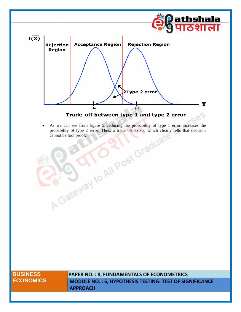
As we can see from figure 5, reducing the probability of type 1 error increases the

probability of type 2 error. Thus, a trade off exists, which clearly tells that decision

cannot be fool proof.

Documents

Subject BUSINESS ECONOMICS Paper No and Title 8