Subcycling in transient finite element analysis

Bruijs, W.E.M.

DOI:10.6100/IR340613

Published: 01/01/1990

Document VersionPublisher’s PDF, also known as Version of Record (includes final page, issue and volume numbers)

Please check the document version of this publication:

• A submitted manuscript is the author's version of the article upon submission and before peer-review. There can be important differencesbetween the submitted version and the official published version of record. People interested in the research are advised to contact theauthor for the final version of the publication, or visit the DOI to the publisher's website.• The final author version and the galley proof are versions of the publication after peer review.• The final published version features the final layout of the paper including the volume, issue and page numbers.

Link to publication

General rightsCopyright and moral rights for the publications made accessible in the public portal are retained by the authors and/or other copyright ownersand it is a condition of accessing publications that users recognise and abide by the legal requirements associated with these rights.

• Users may download and print one copy of any publication from the public portal for the purpose of private study or research. • You may not further distribute the material or use it for any profit-making activity or commercial gain • You may freely distribute the URL identifying the publication in the public portal ?

Take down policyIf you believe that this document breaches copyright please contact us providing details, and we will remove access to the work immediatelyand investigate your claim.

Download date: 31. Jul. 2018

Subcycling in Transient Finite Element Analysis

Het onderzoek in di,t proefschrift werd gedeeltelijk gesteund door de Nederlandse organisatie voor Toegepast Natuurwetenschappelijk Onderzoek- TNO.

The work described in this thesis was partly spousored by the Netherlands Orga.nization for Applied Scientific Research- TNO.

CJP-GEGEVENS KONINKLIJKE BIBLIOTHEEK, DEN HAAG

Bruijs, Willern Elisabeth Maria

Subcycling in tra.nsient finite element a.nalysis I Willem Elisabeth Maria Bruijs. -[SJ. : s.n.] Proefschrift Eindhoven. - Met lit. opg. ISBN 90-9003684-9 SISO 515 UDC 517.9(043.3) Trefw.: eindige elementen methode I numerieke integratie.

Subcycling in Transient Finite Element Analysis

PROEFSCHRIFT

ter verkrijging van de graad van doctor

aan de Technische Universiteit Eindhoven,

op gezag van de Rector Magnificus, prof.ir. M. Tels,

voor een commissie aangewezen door het College van Dekanen

in het openbaar te verdedigen

op vrijdag 9 november 1990 om 14.00 uur

door

Willem Elisabeth Maria Bruijs

geboren te Bergen op Zoom

druk: wibro dlssertatiedrukkerlj, helmond.

Dit proefschrift is goedgekeurd door de promotoren:

Prof. dr. ir. J.D. Janssen Prof. dr. ir. A.M.A. van der Heijden

Copromotor:

Dr. ir. A.A.H.J. Sauren

Voor mijn vader

CONTENTS

ABSTRACT 9

SAMENVATTING 11

1 INTRODUCTION 13 1.1 Goal of the Work 13 1.2 Structure of this Thesis 17

2 NUMERICAL INTEGRATION OF ORDINARY NONLINEAR 19 DIFFERENTlAL EQUATIONS 2.1 Introduetion 19 2.2 Governing Equations 19 2.3 lmplicit Methods 21 2.4 Explicit Methods 25 2.5 Discussion of Explicit and lmplicit Methods 26 2.6 EXpected Computer-Time Savings Due to Subeycling 30

3 SUBCYCLING 33 3.1 Introduetion 33 3.2 Assumptions Due to Subeyeling 34 3.3 Implementation in the PISCES-3DELK Program 45 3.4 Optimization of the Group Partitioning 48 3.5 Stability of the Subcycling Algorithm 50 3.6 Contact 5"2 3.7 Test Examples 53

4 ACCURACY ASPECTS 63 4.1 Introduetion 63 4.2 Dispersion 65 4.3 Oversboot 69 4.4 Subeycling 71

5 OUT-OF-POSITION AIRBAG V ALlDATION TESTS 75 5.1 Introduetion 75 5.2 Test Description 76 5.3 Results 80

7

6 SIMULATION OF THE DRIVER SIDE AIRBAG OUT-OF-POSITION 83

TESTS 6.1 Introduetion 6.2 Model Setup 6.3 Results 6.4 Discussion and Conclusions

7 SIMULATION OF THE PASSENGER SIDE AIRBAG

OUT-OF-POSITION TESTS 7.1 Introduetion 7.2 Model Setup 7.3 Results 7.4 Discussion and Conclusions

8 CONCLUSIONS 8.1 Introduetion 8.2 Subcycling 8.3 Simulations and Validation Tests 8.4 Concluding Remarks ·

REFERENCES

APPENDICES

NOTATION AND SYMBOLS

8

83 83

86 90

93

93 ' 93

97

100

105 105 10$ 106 107

109

115

133

ABSTRACT

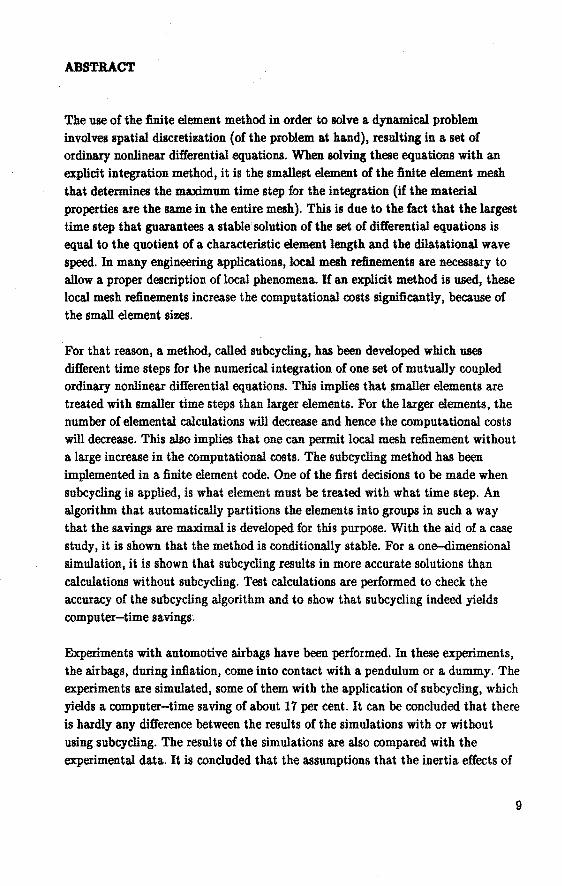
The use of the finiie element metbod in order to solve a dynamical problem involves spatial discretization (of the problem at hand), reauiting in a set of ordinary nonlinear differential equations. When solving these equations with an explicit inlegration method, it is the smallest element of the finite element mesh that determines the maximum time step for the integration (if the material properties are the same in the entire mesh). This is due to the fa.ct that the largest time step that guarantees a stabie solution of the set of differential equations is equal to the quotient of a characteristic element length and the dilatational wave speed. In many engineering applications, local mesh refinements are necessary to allow a proper description of local phenomena. If an explicit metbod is used, these local mesh refinements increase the computational costs significantly, because of the small element sizes.

For that reason, a method, called subcycling, has been developed which uses different time steps for the numerical integration of one set of mutually coupled ordinary nonlinear differential equations. This implies that smaller elements are treated with smaller time steps than larger elements. For the larger elements, the number of elemental calculations will decrease and hence the computa.tional costs will decrea.se. This also implies that one can permit local mesh refinement without a large increa.se in the computational costs. The subcycling metbod ha.s been implemented in a. finite element code. One of the first decisions to be made when subcycling is applied, is what element must be trea.ted with what time step. An algorithm that automatically partitions the elements into groups in such a way that the savings are maximal is developed for this purpose. With the aid of a case study, it is shown that the metbod is conditionally stable. Fora one-dimensional simulation, it is shown that subcycling results in more accurate solutions than calculations without subcycling. Test calculations are performed to check the accuracy of the su:bcycling algorithm and to show that subcycling indeed yields computer-time savings~

Experiment& with automotive airbags have been performed. In these experiments, the airbags, during inflation, come into contact with a pendulum or a dummy. The experiments are simulated, some of them with the application of subcycling, which

yields a computer-time saving of about 17 per cent. It can be concluded that there is hardly any difference between the results of the simulations with or without using subcycling. The results of the simulations are also compared with the experimental data. It is concluded that the a.ssumptions that the inertia effects of

9

the gas and the pressure gradients of the gas inside the airbag can be neglected, lead to incorrect results for some of the simulations. That is why one of these experiment& is also simulated with a model for which these assumptions are not made. This yields ~tter results.

10

SAMENVATTING

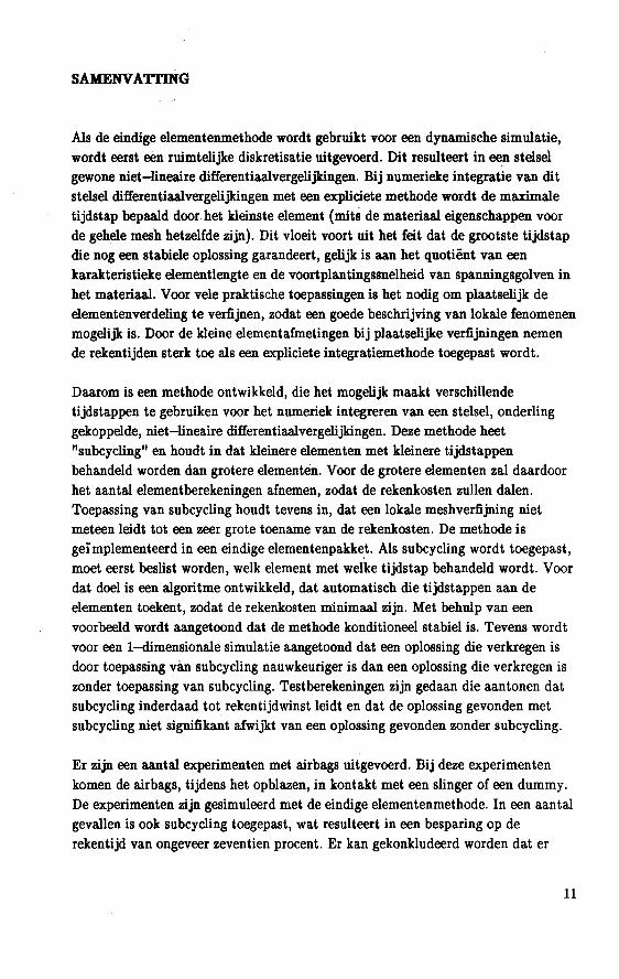
Als de eindige elementenmethode wordt gebruikt voor een dynamische simulatie, wordt eerst een ruimtelijke diskretisatie uitgevoerd. Dit resulteert in een stelsel gewone niet-lineaire differentiaalvergelijkingen. Bij numerieke integratie van dit stelsel differentiaalvergelijkingen met een expliciete methode wordt de maximale tijdstap bepaald door het kleinste element (mits de materiaal eigenschappen voor de gehele mesh hetzelfde zijn). Dit vloeit voort uit het feit dat de grootste tijdstap die nog een stabiele oplossing garandeert, gelijk is aan het quotiënt van een karakteristieke elementlengte en de voortplantingssnelheid van spanningsgolven in het materiaal. V oor vele praktische toepassingen is het nodig om plaatselijk de elementenverdeling te verfijnen, zodat een goede beschrijving van lokale fenomenen mogelijk is. Door de kleine elementafmetingen bij plaatselijke verfijningen nemen de rekentijden sterk toe als een expliciete integratiemethode toegepast wordt.

Daarom is een methode ontwikkeld, die het mogelijk maakt verschillende tijdstappen te gebruiken voor het numeriek integreren van een stelsel, onderling gekoppelde, niet-lineaire differentiaalvergelijkingen. Deze methode heet "subcycling" en houdt in dat kleinere elementen met kleinere tijdstappen behandeld worden dan grotere elementen. V oor de grotere elementen zal daardoor het aantal elementberekeningen afnemen, zodat de rekenkosten zullen dalen. Toepassing van subcycling houdt tevens in, dat een lokale meshverfijning niet meteen leidt tot een zeer grote toename van de rekenkosten. De methode is geïmplementeerd in een eindige elementenpakke.t. Als subcycling wordt toegepast, moet eerst beslist worden, welk element met welke tijdstap behandeld wordt. Voor dat doel is een algoritme ontwikkeld, dat automatisch die tijdstappen aan de elementen toekent, zodat de rekenkosten minimaal zijn. Met behulp van een voorbeeld wordt aangetoond dat de methode konditioneel stabiel is. Tevens wordt voor een !-dimensionale simulatie aangetoond dat een oplossing die verkregen is door toepassing vàn subcycling nauwkeuriger is dan een oplossing die verkregen is zonder toepassing van subcycling. Testberekeningen zijn gedaan die aantonen dat subcycling inderdaad tot rekentijdwinst leidt en dat de oplossing gevonden met subcycling niet signifikant afwiJ"kt van een oplossing gevonden zonder subcycling.

Er zijn een aantal experimenten met airbags uitgevoerd. Bij deze experimenten

komen de airbags, tijdens het opblazen, in kontakt met een slinger of een dummy. De experimenten zijn gesimuleerd met de eindige elementenmethode. In een aantal gevallen is ook subcycling toegepast, wat resulteert in een besparing op de

rekentijd van ongeveer zeventien procent. Er kan gekonkludeerd worden dat er

11

nauwelijks verschil is tussen de resultaten va.n simulaties met en zonder subcycling. De simulatie resultaten zijn ook vergeleken met de experimentele gegevens. Uit deze vergelijking ka.n gekonkludeerd worden dat de aannames dat traagheidseffekten en drukgradiënten va.n het gas in de airbag verwaarloosd kunnen worden, voor sommige simulaties tot foutieve resultaten leiden. Daarom is een van deze experimenten ook gesimuleerd met een model waarbij deze aannamen niet zijn gedaan. Dit leidt tot een betere overeenstemming met resultaten va.n de experimenten.

12

1 INTRODUCTION

1.1 Goal ofthe Work

Analyses with tra.nsient finite element method.s eome from different a.pplica.tion fields, such a.s fluid-structure intera.ction, fluid flow, aircra.ft and vehicle structure design, cra.shworthiness and a.erodyna.mics, nuclear physics, electromagnetics, whea.ther foreca.sting etc. One thing that all problems to he analyzed have in common, is that one ha.s to deal with large structures. Furthermore, in some area.s large gra.dients of the unknowns are expected. This implies that in these area.s a fine finite element mesh is necessary, yielding large numhers of degrees offreedom. For many applications, the constitutive equa.tions of the fluid or the structure are highly nonlinear. This willlead to computer-times which, are aften far too high to apply transient finite element analysis a.s a tooi for design or parameter studies. The purpose of this work is the reduction of the computer-time necessary for large scale transient finite element analysis. Since the problem statement originates from the field of vehicle crashworthiness, the attention in the discussion following below, will he focussed on this field.

Automobile manufacturers aften use full scale crash tests in order to establish the crashworthiness of their vehicles, and the influence of a crash on the accupants of the vehicle. At present an airbag is aften included which inflates shortly after the crash and protects the accupants from impact with the steering wheel and partsof the interior. Fu11 scale crash tests suffer from a number of problems. First, they ca.n only be applied in the :fi.nal stages of the design process. If structural changes to the vehicle are necessary, a new test must he performed. It would he helpful if it were possible to get information about the crashworthiness of the vehicle in an early stage of the design process. Another problem is that the tests are very costly. This is due to the relatively expensive prototypes that are aften used for the tests, a.s well as to the time needed for the preparation of the vehicles and for the processing of the huge amount of test data. Also, for practical reasons, the number of measured qua.ntities is limited.

The numerical simulation of a vehicle crash does not suffer from the first problem. It can be performed in an early stage of the design process. Furthermore, all · quantities that interfere with the total crash behaviour, must be calculated. This means that aftera crash simulation more information is available compared with a crash test. Another important advantage of crash simulation is the possibility of parameter studies that can he performed quite ea.sily.

13

The simulation of a full scale crash involves: - large displacements; - large deformations; - plastic material behaviour; - complicated contact phenomena (not only beiween the vehicle and the harrier,

but also between different partsof the vehicle); - time integration.

Due to these aspects, the performance of a full scale crash simulation costs a lot of computer-time, typically in the order of twenty hours on a supercomputer. Furthermore, the generation of the fini te element model of the vehicle structure is rather time consuming, something in the order of five hundred man-hours. The state of the art of full scale crash simula.tion is described by Haug et al. (1988) and Haug & Ulrich (1989) and the results seem promising (fig. 1.1). A problem that occurs during the modelling of the structure is the fact that it is very difficult to describe welding spots and other connections. A very important advantage of full scale crash tests on the other hand, is that it is not necessary to make a model of the structure, so no assumptions have to be introduced.

These aspects lead to the fact that the costs of the simulations will often be too high to ap:ply crash simulation as an efficient and versatile design tooi, especially if in the simulation also the accupants and airbags are included.

If the computer-times can be reduced, crash simulation can be applied more efficiently and economically in the design process. Of course, crash tests will always be necessary to validate the model, but after proper validation, crash simulation is a tooi that can be used for parameter studies and as a result, the number of tests will decrease.

As mentioned before, the purpose of the present study is the development of numerical tools that will decrease the computer-time necessary for transient finite element analysis. This discussion shows that for crashworthiness studies, computer-times are too high. Similar argumentscan be given for other fieldsof application.

Some methods that are available to reduce computer-times are: - the use of vector and parallel computing; - the use of "super elements"; - improvements in time integration methods.

14

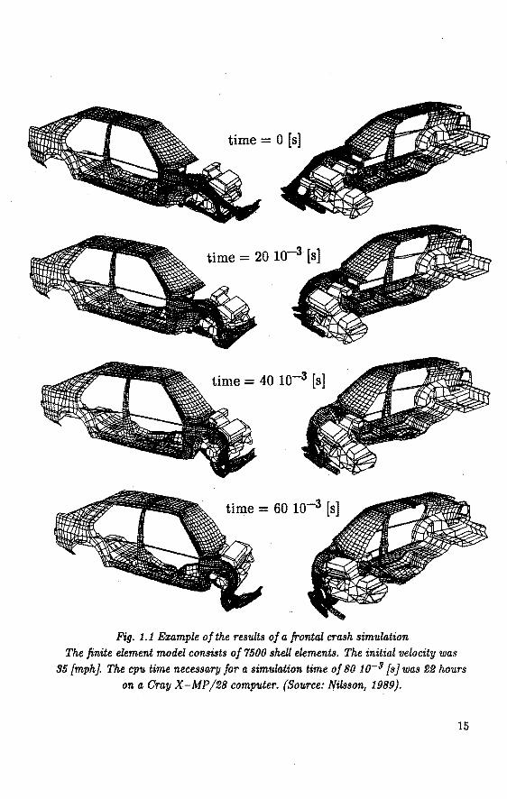
time= 0 [s]

time= 20 10-3 [s]

time = 40 10-3 [s]

time= 60 10-3 [s]

Fig. 1.1 Example of the results of a frontal crash simulation The finite element model consists of 7500 sheU elements. The initial velocity was

95 {mph}. The cpu time necessary fora simwation time of 80 10-3 [s] was 22 hours

on a Gray X-MP/28 computer. (Source: lfilsson, 1989).

15

Due to the rapid development of fast vector and parallel computers, a lot of work is doneon vectorization and parallelization of the computer programs ( Ginsberg & Johnson, 1989; Ginsberg & Katnik, 1989). This yields large computer-time savings which are computer dependent. If another computer is used, changes in the program are necessary in order to optimally use the vector andfor parallel features of the specific machine. This thesis will not deal with vectorization and parallelization, however, the implementation of the developed tools is performed in such a way that the vectorization of the code is not disturbed.

The second metbod uses knowledge of the behaviour of the components of the structure. For instance, the impact of a component of the vehicle stucture can be analysed stand alone using the finite element method. The resulting force-displacement rela.tion for this component, can be used in a full sca.le crash simulation. The advantage is that the results of the component simulation can be used in a number of full sca.le crash simulations, which leads to computer-time savings. Disa.dvantages are that contact between the component and other parts of the vehicle structure cruinot be taken into account and when changes are made in the geometry of the component, a new force-displacement relation must be derived. '

This study will focus on the third method, the impravement of time integration methods because, as will be shown in chapter 2, a computer-time saving can be expected by a.daptation of the standard integration methods. It is remarked that the impravement of the time integration methods described in this thesis can be combined with the otber metbods to reduce the computer-times, to result in even larger savings.

In genera.l, the st.roeture of which the crashworthiness must be verified bas a complicated geometry. For this reason, the finite element metbod is commonly used in crash simulation for tbe spatia.l discretization of tbe structure. If tbe fini te element metbod is applied, tbe momentnm equations (whicb are partia.l differentia.l equations ), tbe constitutive equations and tbe relations between tbe deformations and the displacements are transformed into a set of ordinary nonlinear differentia.l equations (Bruijs, 1987). This set of differential equations with the given initia.l conditions can be solved by numerical integration.

Basically, there are two metbods to integrate sets of ordinary nonlinear differentia.l equations: explicit and implicit metbods. If an implicit method is applied, the ca.lculation of the relevant quantities at the new point in time, requires quantities at this new point in time. If an explicit metbod is applied, the relevant quantities

16

at the new point in time can be calculated from quantities at earlier points in time · exclusively. As shown in chapter 2, the advantage of the explicit methods is their simplicity. lt is not necessary to solve sets of coupled equations. In exchange for the simplicity of the explicit methods, the time step used for the integration is bounded by the Courant criterion (Courant et al., 1928) to eneure stability. A · metbod is called stabie if the solution obtained with the method is bounded. The results of an unstable calculation are useless. If an implicit method is used, for each time step a set of nonlinear equations must be solved. This means that ihe costs per time step and the storage requirements are high and tend to increase dramatically with the size of the fini te element mesh. But implicit methods are often unconditionally stable, which means that there is no upper bound to the time step based on stability conditions. The time step can be chosen on grounds that are determined by accuracy demands only. For both implicit and explicit methods, a lot of integration schemes have been developed. For an overview of schemes that are often used in structural dynamica! analysis, it is relerred to Belytschko & Bughes (1983). All these schemes have their particular advantages and disadvantages.

The method called subcycling uses an explicit integration scheme as a basis. This integration scheme is ada.pted in such a wa.y tha.t the disadvantages of the explicit scheme beoome less apparent. Application of the subcycling method implies that small time steps are only used in areas where stability requirements demand them. In other areas, much larger time steps will be used. Though, as will be shown, subcycling is particularly suited for crash simulation, it can also be used in other fields of application.

1.2 Strodure of this Thesis

In chapter 2, the two basic numerical methods to integrate sets of ordinary nonlinear differential equations are treated. Their applicability to crash simulation is inferred from tlie advantages and the disadvantages of the methods. It is concluded that explicit methods are most suited for crash simulation. It is also explained why subcycling will yield computer-time sa.vings and under what conditions these savings will be maxima!.

In chapter 3, the problems which occur when subcycling is applied are treated. Different alternatives for the solution of these problems are compared with respect to numerical stability and accuracy. One of the alternatives is chosen and implemented in the PISCES-aDELK finite difference/finite element package (PISCES-3DELK Users Manual, 1990) for a tria.ngular constant strain membrane

17

element. Before subcycling ca.D be applied, it must be decided what elements are integrated with what time step. An optimizaiion algorithm which fully automatically finds the group division that yields the largeat computer-time saving will be deacribed. The stability of the subcycling algorithm is diacussed. In many problems, contact is expected to occur. Adaptations necessary for subcycling to the &ntact algorithms will be discussed. Finally, the reaults of some teat calculations will be presented.

Chapter 4 deals with the accuracy of the subcycle method. Using a simple one-dimensional problem, it is shown that a soluiion obtained with subcycling is more accurate than a solution obtained with a conveniional integration method, using one time step for the entire meah.

Experiment& are performed which concern the inflation of an automotive airbag. During infla.tion, the airbag will hit a pendulum or a dummy. Due to interaction with the airbag, the pendulum and the dummy are accelerated. The experiments are described in chapter 5. The results will be presented in the chapters 6 and 7, together with the results of the numerical simulations of these experiments.

The experiments mentioned above have been simulated using the PISCE8-3DELK finite element/finite difference code with the subcycling option for the simulation of the inflating airbag and the MADYMO code (MADYMO Users Manual 3D, 1988) for the simula.tion of the beha.viour of the pendulum and the dummy. The MADYMO program is a crash victim simula.tion program based on multibody dynamica. It can be used to simulate the beha.viour of systems of rigid bodies. The rigid bodies are connected to each other by joints. The motion of the systems of rigid bodie8 is constituted by external forces acting on the bodies. A coupling

between the PISCES-3DELK code and the MADYMO code (Buijk, 1989) is available in order to account for the interaction between the airbag and the pendulum or the dummy. In the chapters 6 and 7, tbe model of the experiment&, used for the simula.tion, is discussed and the results of the simulations are presented together with the experimental results, for the driver side airbag and the passenger side airbag reapectively.

In chapter 8, the performance of the subcycling algorithm is discussed. Also the

reaults of the simulations of the experiments with the airbag are discussed. Finally, conclusions are drawn and some recommendations for future research are given.

18

2 NUMERICAL INTEGRATION OF ORDINARY NONLINEAR DIFFERENTlAL EQUATIONS

2.1 Introduetion

In this chapter, the numerical integration techniques used to solve ordinary nonlinear differential equations will be described. First, in section 2.2, the momenturn equation, which is a partial differential equation, the constitutive equation and the strain-displacement relation are combined to obtain a set of ordinary differential equations using the finite element method for spatial discretization. For the solution of this set of ordinary differential equations, there are basically two kinds of integration methods: explicit and implicit methods. A method is called explicit if, for the determination of the displacements and the velocity at the new point in time only quantities are necessary at previous points in time. An impHeit method also needs quantities at the new point in time in order to calculate the displacements and the veloeities at the new point in time. As an example of the implicit methods, the Newmark-P method {Newmark, 1959) is chosen. This method is discussed insection 2.3. Insection 2.4, an example of an explicit method, the central difference method {Bathe & Wilson, 1976) is discussed. The advantages and disadvantages of explicit and implicit methods are

weighed against each other in section 2.5. It is shown that for many engineering applications neither implicit, nor explicit methods are entirely suitable for the integration of the set of differential equations. That is why special methods which combine the features of different integration schemes have been developed. Some of these methods will be discussed. One of them is subcycling. In section 2.6, it is shown that subcycling may yield substantial savings in computer-time for many engineering applications, such as fluid-tltructure interaction, fluid flow problems, studies to the aerodynamics of vehicles and crash simulation.

2.2 Governing Eqilations

In the absence of thermomechanical effects, the behaviour of a structural system can bedescribed with the momenturn equation:

.... -V· a+ pq= px (2.1)

the constitutive equation:

a= o(E{t)) (2.2)

19

the relation between the deformations and the displacements:

E = E(F) (2.3)

the boundary conditions on the outer surface A of the structural system:

~knownonAk {2.4)

pel= a·n known on Ad (2.5)

and the initial conditions:

i(t = 0) and i(t = 0) known (2.6)

... with i the displacement vector, V the gradient operator, related toa relerenee configuration and defined by:

-1

di·VVJ = VJ(i +di)- VJ(i) (2.7)

with tp a place-dependent scalar quantity and di an arbitrary infinitesimal change of the displacement vector, a the stress tensor, p the density, q the body force per unit mass, E the strain tensor and F the deformation tensor defined by:

(2.8)

A k is the pá.rt of the outer surface A of the structural system to which kinematica! bounda.ry conditions apply and Ad the remaining part of the outer surface to which dynamica! boundary conditions apply. The vectornis the outer normal vector on the surface and pd are the known external forces. A superposed dot denotes the partial time derivative. In these equations, a, p, q, i, E and F are functions of the , position in the structural system and the time t. With the finite element method, these equations are spatially discretized and transformed into a set of ordinary nonlinear differential equations (Bruijs, 1987) yielding:

Mi= fext(x,t) -fint(:!!;,i,t) (2.9)

with M the constant mass matrix, ! a column matrix containing tlJ.e nodal displacements, fini a column matrix containing the nodal internal forces, which are a function of the nodal displacements, the nodal veloeities and time and fext the

20

column matrix containing the nodal exiernal fotces that are a function of time and ihe nodal displacements. Thai the external fotces are a funciion of the nodal displacements is due to the fact that cantacts beiween the structural system and its surroundings and cantacts between paris ofthe structutalsystem mutually, are allowed. This set of di:fferential equaiions, tagether with the boundary conditions and the initia! condiiions deseribe the behaviour of the discretized structural system.

Thesetof di:fferential equations (2.9) is nonlinear. There are three sourees of nonlinearities: - physical nonlinearities (nonlinear material behaviour), - geometrical nonlinearities (large displacements), - nonlinearities in the external forees (contacts). The physical and geometrical nonlinearities are taken care of by the fini te element method. For the contacts, section 3.6 is referred to.

2.3 Implicl.t Methods

Because the purpose of this and the following section is only to illust,rate the advantages and disadvantages of implicit and explicit integration techniques, it is assumed that the internal forees at time t are only a funciion of the displacements at time t and the external fotces are known functions of time and do not depend on the nodal displacements.

In numerical integration, the quantities are caleulated at a number of discrete points in time At, 2At, ... nAt. For reasans of simplicity, it is assumed that these points are equally spaeed in time. The following notation convention is introduced~ a subscript denotes the point in time at which a quantity is considered, e.g. ~ denotes the column of the nodal dispaeements at time nAt, fint 1 denotes the column of the nodal internal farces at time At etc.

Let thesetof di:fferential equations to be solved be denoted as:

(2.10)

and let .io and io be known. Fot reasans of notaiion, the time dependenee of the forcesis not indicated. This initial value problem can be solved With an implicit integration technique. As an example of an implicit integration technique, the Newmark-P method (Newmark, 1959) will be discussed. The relations for the Newmark-P metbod are:

21

~+t =~+at in+ at2( (~- P> in+ Pin+l)

in+ I =in+ .àt [(1 -fJ)in + 1J in+t]

(2.11)

(2.12)

The par~eters 11 and p can be chosenon the intervals (0,1] and (0,1/2] respectively. The case in which 11 = 0 and/or p = 0 is excluded from this discussion, because forthese valnes the method is explicit. For other values of 'fJ

and p, the method is called implicit because the displacements and veloeities at time (n+1)6t are not only a function of the quantities at time nAt, but also of the accelerations at time (n+1)6t. Consider (2.10) at time (n+1)At:

(2.13)

Let the nodal displacements, veloeities and accelerations be known at the discrete points in time up to and including time nAt. Herealter itrwill be described how these quantities can be calculated at time (n+1)At using the Newmark-P scheme (2.11) and (2.12) and the differential equation (2.13). Equation (2.11) can be transformed into:

1 ~

--P - 1( ) 1. 2 .. ~+1 =-- ~+~-~ - -~- --~

PAt2 PAt P

Substitution of (2.14) in (2.13) yields:

(2.14)

(2.15)

This is a set of nonlinear equations from which ~+1 can be solved using standard numerical techniques (Bathe & Wilson, 1976). Substitution of ~+l in (2.14) yields in+1· Substitution of in+l in (2.12) yields in+1· Now all quantities at time (n+1)6t are known. The same calculations can be performed to find the values of the quantities at (n+2)At etc.

To start, (2.10) is considered at time zero. The known initia! values !o and ~are substituted in (2.10) to calculate io· If !(), io and io are known, the strategy described above can be used to calculate ~1 • Hence, no special starting algorithm is

22

necessary.

Stahility and Aceuracy

The stability and the accuraey are derived for an undamped linea.r system, so fint

can he written as K 11;:

Mi+Kx=fm. (2.16}

where K is the stiffness matrix. These equations can he written in the diagonal

form (Bathe & Wilson, 1976):

i+!h;=.Y:fext (2.17}

where Y is the matrix containing the M-orthonormalized eigencolumns y and ll is the diagonal matrix containing the eigenvalnes W2 of the generalized eige~problem:

(2.18}

To study the stability and the accuracy of integration schemes, the attention can

he focussed on one equation of thesetof uncoupled differential equations (2.17):

i+W2x=f

For each specifi.c integration scheme, a recursive relation exists of the form (Hughes, 1983):

(2.19)

(2.20)

The elements of the column y, the matrix :R and the column g depend on the integration scheme used. For an example of the contents of the column y, it is

referred to appendix A. The matrix :R is usually called the amplifi.cation matrix

(Hughes, 1983). Let Pi be the eigenvalnes and l'!i he the eigencolumns of :R. Let the initia! valnes of (2.16) he stored in the column Yo· These initia! valnes can he

written as a linea.r combination of the eigencolumns l'!i:

k Yo = E a. l'!·

i=1 1 1 {2.21)

where kis the numher of elementsof the column y. Combination of {2.20) and

23

(2.21} yields:

k I1 = E ~ IJi l!ï + !lo

i=l

From the above, it ca.n be inferred that the expression for In must have a contri bution of the form:

k E a. Jlt W·

i=l 1 I -"-1

or, if notall J.li are distinct, a contribution of the form:

k-1 . El~ #'Ï l!ï + n ak ~lik 1=

(2.22)

(2.23)

(2.24)

where it is a.ssumed that l"k is equal to one of the J.li (i= 1, ... , k-1). Define the speetral radius of the matQx R, p

8(R) as (Hughes, 1983):

(2.25)

An integration metbod is ca.lled stabie if IIInll is bounded. From (2.24) it ca.n be deduced that an integration metbod is stabie if the following conditions are both satisfied:

- P8(R) ~ 1; - eigenvalnes with multiplicity greater tha.n one are less than one in modulus.

Due to the complicated nature of the matrix R for the Newmark-,8 method, the determination of the speetral radius of Ris rather complex. Therefore in this thesis only the results of the stability analysis are given. For more details it is relerred to Rughes (1983). The Newmark-,8 method is unconditionally stabie if:

1 2a>., >­fJ- ., - 2

and conditionally stabie if:

and:

24

(2.26)

(2.27)

1 P<-r,

2 (2.28)

In tbe case of conditional stability, an additional requirement must be satisfied:

A Wcrit ~t<-­- w

(2.29)

where:

wcrit = <~-m-1/2 {2.30)

The additional condition (2.29) must be satisfied for eacb mode in tbe mesh. So w is the maximum frequency in tbe mesb.

Tbe local truncation error Re is defined as tbe error made by tbe time discretization. It can be written in tbe form (Hughes, 1983):

R = c fl.tP+l e (2.31)

wbere pis tbe order of tbe metbod by definition. For tbe Newmark-P metbod it

may be argued that p = 2 if 1J = 1/2 and p = 1 otberwise (Hugbes, 1983).

2.4 Explicit Methods

Suppose tbat tbe differential equa.tion to be solved is once again given by (2.10) and tbe initial conditions are (2.6). This initial value problem can also be solved

witb explicit integration tecbniques. An often used explicit integra.tion metbod is

tbe so-called central difference metbod (Batbe & Wilson, 1976):

. - . !l.t x ~+1/2 - ~-1/2 + -n (2.32)

~+1 = ~ + !l.t in+l/2 (2.33)

This metbod is called explicit beca.use tbe positions and veloeities at the times

(n+l)!l.t and (n+1/2)At, respectively, can be c8.lculated from qua.ntities at

previous points in time only. Consider (2.10) at time nAt:

{2.34)

Let tbe nodal positions be known up to and including tbe point in time n!l.t and

25

tbe veloeities up to and including (n-1/2)~t. Next (2.34) can be used to calculate the nodal accelerations at time n~t. Equation (2.32) can be used to calculate

in+l/2 and (2.33) to calculate Xn+l' Tben (2.10) is considered at time (n+l)M and used to calculate in+ 1 etc. Tbe initial velocity is given at time zero. To be able to apply (2.32) for tbe first time, tbe velocities at time -~t/2 must be known. Possible metbods are:

(2.35)

or:

~-1/2 = ~ (2.36)

Stability and Accuracy

Tbe central difference scbeme can also be written in tbe form {2.20). Because this metbod will be used later for tbe subcycling algorithm, in appendix A tbe stability of tbe central difference metbod is derived. Tbe central difference metbod is stabie if:

2 ~t <­-w (2.37)

wbere wis tbe maximum frequency appearing in tbe mesh. Eq. (2.37) is the so-ealled Courant criterion (Courant, 1928). Fora linear 2-noded element, it can be deduced tbat (Belytschko, 1980b):

(2.38)

where cis the dilatational wave speed and lis tbe lengtbof tbe element. In that case, (2.37) can be written as:

~t ~ 1/c

Tbe local truncation error of the central difference method is of tbe order 2 (Hugbes, 1983).

2.5 Discussion of Explicit and lmplicit Metbods

(2.39)

H tbe mass matrix is diagonal, the central difference method does not involve the

26

solution of sets of coupled equations in order to obtain the nodal accelerations. In . general1 however1 the mass matrix is not diagonal. It can be made diagonal by a technique called lumping. Physically 1 this means that the mass of the elements is concentrated in the nodes. Krieg & Key (1973) have shown that the errors of the central difference method and mass lumping are compensatory 1 so mass lumpirig is preferabie to the use of consistent mass matrices. Hereafter it is assumed that the mass matrix is diagonal, so the a.pplication of the central difference metbod does not involve the solution of sets of coupled equa.tions1 in contrast with the Newmark-P method. If the Newmark-P method is applied1 at each time step a set of nonlinear coupled equa.tions must be solved. This implies extra core storage and computer-time. The costs per time step for the Newmark-P method increase dramatically with the size of the mesh. In exchange for iis simplid ty 1 the central difference metbod is only conditionally stabie and therefore the time step must be small. The Newmark-P metbod is unconditionally stabie if the parameters 'fJ and p are chosen properly. The time step is then bounded by accuracy demands only.

It can be concluded that for the Newmark-,8 method1 or for implicit methods in general1 the costs per time step are high, but the time step is not bounded by sta.bility criteria. For the central difference method, or for explicit methods in general1 the costs per time step are low, but numerical stability requires the use of small time steps.

In a. crash simulation, the total number of degrees of freedom is large. For exa.mple1 Hoeck (1988) used 30.000 elements fora full scale side impact simulation. This means tha.t the disa.dvantage of implicit methods - the necessity to solve sets of nonlinear coupled equations - becomes crucial.

In a crash simula.tion, the deformations take place in a small time interval. The duration of a irontal crash is about 150 10-3 [s]. This means that the strain rates wi1l be large. Because the material behaviour is highly nonlinea.r, the time step must be small in order to ensure the correct calculation of stresses. This means that the disadvantage of the central difference metbod - the necessity of a small time step due to sta.bility requirements - turns out to be less apparent. It can be concluded tha.t explicit methods are most suited for crash simulation. For tha.t reason, in most crash codes, a.n explicit integra.tion scheme is a.pplied.

However, fora. particular set of ordinary nonlinear differential equa.tions it is not generally true that one scheme - either explicit or implicit -is perfectly suita.ble for the integra.tion of the set of differential equa.tions. Because of the ma.ny different finite element types and local mesh refinements used in large scale

27

engineering systems, neither of the integration schemes wiJl be vecy efficient by itself. Thatis the reason why methods have been developed in which it is attempted to simultaneously combine the advantages of different integration schemes, or to allow different time steps when using the same integration scheme. These methods are called mixed methods or mesh partit.ions. Basically there are three classes of mixed methods: implicit-implicit (I-I) partitions, explicit.-implicit (E-I) partitions and explicit-explicit (E-E) partitions.

1-1 partitions

As mentioned before, if an implicit metbod is used for the integration, a set of equations must he solved. This can either be done by direct solution or by iterative methods (Bathe & Wilson, 1976). The iterative methods require lesscore storage, but for structural meshes the convergence rateis very poor (Belytschko et al., 1979). In a tluid-structure problem, a direct solution metbod would require too much core storage due to the large size of the tluid meshes. If an îterative metbod is used, the structural mesh will cause a poor convergence rate. So for an effective treatment, an itera.tive metbod is used in the fluid mesh and a direct solution procedure in the structural mesh. This procedure is called a.n 1-1 partit.ion (Park et al., 1977). Examples of problems for which these partitions may be effective are fluid-structure interaction and studies of the behaviour of structures under explosive loads for which the explosion is modelled withafluid mesh.

E-1 partitions

Another possibility is" to integrate the structure implicitly and the tluid mesh explicitly. The relatively large stiffness of the st.roeture wiJllead to very small time steps if the structure is integrated explicitly. The lar~ size of the fluid mesh makes impHeit methods unsuitable. A lot of research bas been done in the field of the E-1 partitious. The partitions were first proposed by Belytschko & Mullen (1977). The stability of these partitions has been studied in Belytschko & Mullen (1978). The nodes are partitioned into two groups, nodes which are integrated with an explicit scheme and nodes which are integrated with an impHeit scheme. The elements that contain nodes which are integrated explicitly as well as nodes which are integrated implicitly - called interface elements - require a special treatment. Therefore, the elements have to be partitioned into three groups, i.e. explicit elements, implicit elements and interface elements. The explicit nodes are integrated first and the results are used as boundary conditions for the implicit nodes. Bughes & Liu (19788 •b) proposed a.n alternative E-1 partition for linear problems which is easier to implemerit. In their approach, the elements are divided

28

in only two groups: explicit and implicit element&. The coupling between the groups is accounted for by the usual fini te element aasembly procedure. In Bughes et al. (1979), this partition is extended to nonlinear transient analysis. In Park {1980) and Park & Felippa. (1980), respectively, the sta.bility a.nd the accuracy of a general partitioned procedure is studied. The E-1 partitions a.re further extended by Liu & Belytschko (1982) by allowing different time steps in the explicit and implicit pa.rts. They called these methods mixed time E-1 partitions. The implementa.tion and the accuracy of the mixed time E-1 partitions is studied in Liu, et al. (1984). Application examples of these methods are the sa.me ones as for the I-1 partitions. The difference in performance between the I-I and E-I partitions depends on how bad the convergence ra.te of the structural mesh will be and the number of elements in the structural and the fluid mesh.

E-E partitions

If a structural mesh consistsof a stiff pa.rt and a flexible part, or a part with very small elements and a part with larger elements, the stability condition requires a much smaller time step in the first part of the mesh than in the second part. An economical treatment of this problem is the integration of the stiff part or the part with the larger elements with a smaller time step than the remainder of the mesh. This technique is called subcycling. The subcycling methods were first introduced by Belytschko et al. (1979). A more extensive study of these algorithms is found in Belytschko (1980a). The stability analysis haa uptil now been performed only for sets of first order erdinary differential equations by Liu & Lin (1982) and Belytschko et al. (1983a,b, 1984). In these publications, this is often done for the mixed time E-1 partitions mentioned above. A case study of the stability of a subcycling method applied to a set of second order differential equations is included in Belytschko et al. (1979). Typical exa.mples of problems for which E-E pa.rtitions are effective, are all problems for which local mesh refinements are necessa.ry or problems for which locally stiffer parts are present.

In the case of a crash simulation, the mesh consistsof parts with very small elements and of parts with much larger elements. Also the number of elements will be large. From above, it can be concluded that the most suitable partition method forthese problems is the E-E partition. Another fact pleading for E-E partitions is the fact that codes which are generally used for crash simula.tion are, as mentioned earlier1 mostly explicit. If one were to imptement an E-1 method in these codes, the whole structure of the code would have to be changed. This thesis deals with the E-E partitions where one explicit integration scheme is used with different time steps: subcycling. Subcycling is very well suited for problems where

29

local mesh refinements are neeessary, or where part of the mesh consists of stiffer elements. It can thns be nsed for many engineering applications. If subcycling is applied, the larger or more flexible elements can be treated with a larger time step than when a conventional metbod is used. If a conventional metbod is nsed, the smallest or stiffest element determines the time step for all elements of the mesh. Application of subcycling may thus lead to a computer-time reduction.

Moreover, as will be shown in cbapter 4, subcycling can also canse an increase of the accuracy for some applications.

2.6 Expected Computer-Time Savings Due to Subcycling

If an explicit integra.tion metbod like the central difference metbod is used, the time step must satisfy tbe Courant criterion (2.37). Equa.tion (2.39), which holds fora 2-noded. linear displacement element, shows that the time step is linearly dependent on the element length L For membrane and shell element& a similar upperbound for tbe time step can be derived. But for these elements, lis equal to a cbaracteristic lengthof tbe element.

In order to quantify the savings that can be achieved with subcycling, consider a mesh consisting of n, small element& and n1large elements. Let the ratio of the characteristic lengtbs of the large and small elements be equal to a. Let tbe maximum sta.ble time step for the small elements be .6-t. Then the large elements can be integrated with the time step a.6.t. Laterit will be shown that a must be a positive integer. Let the duration of the phenomena to be simulated be Taim and the computer-time necessary to calculate the unknowns for one element Tc. Then the computer-time with subcycling T

8 is equal to:

(2.40)

The computer-time without subcycling TWII is given by:

(2.41)

Define the savings S, due to subcycling, as:

(2.42)

30

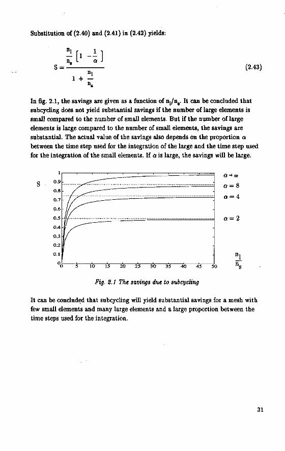
Substitution of (2.40) and (2.41) in (2.42) yields:

(2.43)

In fig. 2.1, the sa.vings are given as a function of n1/n,. U can be concluded tha.t subcycling does not yield substantia.l sa.vings if the num.her of large elements is small compared to the num.her of small elements. But if the num.her of large elementsis large compared to the num.her of small elements, the savings are substantia.l. The actua.l va.lue of the savings a.lso depends on the proportion a between the time step used for the inlegration of the large and the time step used for the integration of the sma.ll elements. If a is large, the savings will be large.

s 0.9

0.8

0.7

0.6

0.5

0.4

0.3

0.2

0.1

0o~-~s~~~o--~1~5~A2~0--~25~-3~o--~3~5--~~~~45~~so·

Fig. 2.1 The savings due to subcycling

a-+oo

a=8

a=4

a=2

It can be conclud~ that subcycling will yield substantia.l savings fora mesh with few sma.ll elements and many large elements and a large proportion between the time steps used for the integration.

31

3 SUBCYCLING

3.1 Introduetion

As will be shown in section 3.2, when subcycling is applied, a problem occurs in elements having nodes which are integrated with different time steps. The displacements of the nodes which are integrated with the large time step will also be necessary at intermedia.te points in time. But they are not available at these points in time. Different choices for the solution of this problem are possible. In section 3.2, several solutions to the problem are given and compared with respect to accuracy and stability.

The best solution is chosen a.nd implemented in the PISCES-3DELK finite difference/finite element packagefora triangular constant strain membrane element in a strain ra.te formulation. The implementation aspects of the subcycling algorithm are presented in section 3.3 using a flow scheme for the computations. For the implementation it is assumed that the master time step, which is the smallest time step used for the integration of the set of differential equations, does not change during the calcula.tion. For some calculations it is desirabie to change this master time step during the calculation. When this subcycling algorithm is applied, this is possible with the restrietion that the master time step can only be changed after an update with the largest time step used for the integration is completed.

Before subcycling can be applied, the elements a.nd the nodes have to be partitioned into groups tha.t will be trea.ted with the same time step. This process is done automa.tically. The user simply bas to specify whether he wants to apply subcycling fora calculation or not. If subcycling is to be applied, an optimiza.tion algorithm, described in section 3.4, determines that group division for which the number of elemental calcula.tions is minimal. Though, up till now, subcycling is only implemented for the constant strain membrane element, the optimization algorithm is capable of handling all other element types. For all calcula.tions which have so far been performed with the subcycling algorithm, the same group partition is used for the entire calculation. There are certain applications for which an adaptation of the group partition during the calculation willlead to a better performance in computer-time. Then the optimization algorithm mentioned a.bove can be used during the calculation to find a new group partition for which the computer--time savings are maximal, given the current deformed mesh of the structure.

33

The stability of several salutions to the problem mentioned above is derived for a linear maaiHipring system. The best solution that was chosen for implementation turned out to be conditionally stabie for this specific casestudy. But the implementation of this salution is performedin combination with a triangular constant strain membrane element. To check the stability behaviour of this salution when applied to the triangular elements, a new case study to the stability is performed using these elements. The results are presented in section 3.5.

In many engineering ptoblems, which are studied with transient finite element analysis, contact will occur. Insection 3.6, it is described how contact can betaken care of in combination with subcycling.

The implemented subcycling algorithm has been applied to a number of test cases. The results of a. selection of these test cases are presented insection 3. 7.

)

3.2 Aasumptions Due to Subcycling

As mentioned before, if subcycling is applied, different time steps are used in different areas of the finite element mesh. In section 2.4 it was described how a set

of ordinary nonlinear differential equations can be solved using an explicit method with the same time step for all differential equations of one set. In the present section different equations of one set of differentiat equations are sol:ved using different time steps. For the integration the central difference method is used, though in principle other methods can be used. Consider eq. (2.9) assuming that the internat forces are a function of the nodal displacements only and the external

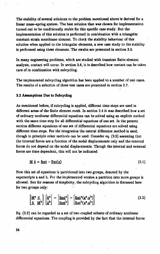
forces do not depend on the nodat displacements. Though the internat and external forces are time dependent, this will not be indicated:

{3.1}

Now this set of equations is parti tioned into two groups, denoted by the superscripts a and b. For the implemented version a partition into more groups is allowed. But for reuons of simplicity, the subcycling algorithm is discussed here for two groups only:

(3.2)

Eq. (3.2) can beregardedas a set of two coupled subsets of ordinary nonlinear differential equa.tions. The coupling is provided by the fact that the internat forces

34

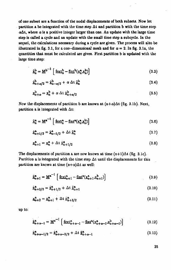
of one subset are a function of the nodal displacements of both subsets. Now let . partilion a be integrated with the time step At and partition b with the time step

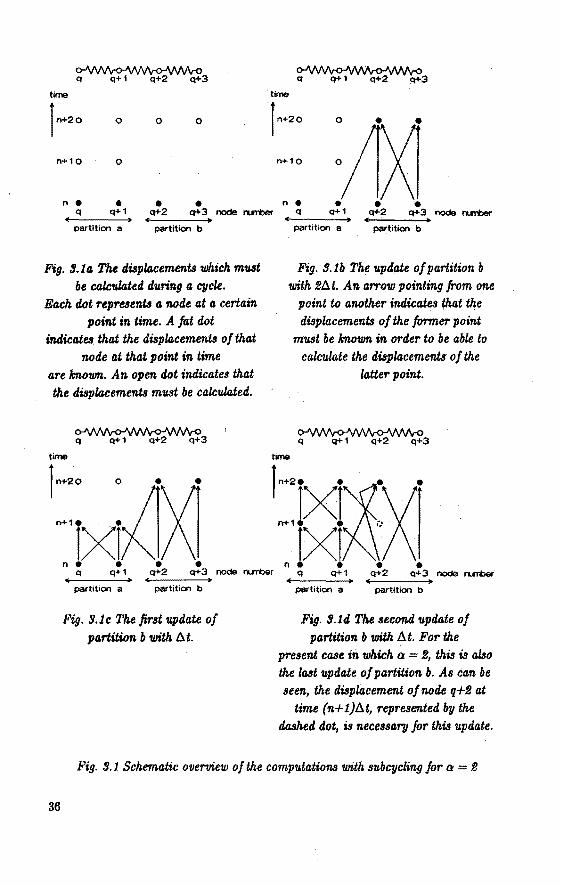
aAt, where a is a positive integer larger than one. An update with the large time step is called a cycle and an update with the small time step a subcycle. In the sequel, the calculations necessary during a cycle are given. The process will also be illustrated in fig. 3.1, fora one-dimensional meshandfora = 2. In fig. 3.1a, the quantities that must be calculated are given. First partition b is updated with the large time step:

~ = Mb-l ( fext~- fin1b(~,~))

~+a/2 = ~-a/2 + a At~

b b A •b ~+a=~ + a .ut ~+a/2

(3.3)

(3.4)

(3.5)

Now the displacementsof parti\ion bare known at (n+a)At (fig. 3.1b). Next, partition a is integrated with At:

(3.6)

i:+1/2 = i:-1/2 + At i~ (3.7)

a a At ·a ~+1 = ~ + L.l ~+1/2 {3.8)

The displacementsof partition a are now known at time (n+1)At (fig. 3.1c). Partition a is integrated with the time step At until the displacements for this partition are known at time (n+a)At as well:

(3.9)

(3.10)

a va At ·a ~+2 = Cn+l + L.l ~+3/2 (3.11)

up to:

(3.12)

(3.13)

35

~ q q+1 q+2 ~3 ~ q ~1 ~2 q+3

time time

1n+20 0 0 0 r n+20

:M n+10 0 n+1o

n • • • • n • • • • q ~1 q+2 ~3 node ruri>er q q+1 ~2 q+3 node ruri>er

partition a partition b

Fig. 9.1a The displacements 'Which must be calculated during a cycle.

Each dot represents a node at a certo.in point in time. A fat dot

indico.tes. tho.t the displacements of that node at that point in time

are known. An open dot indico.tes tho.t the displacements must be calculated.

~ q . ~1 q+2 q+3

time

ln+20 o • •

~·rxi~X n • • • • q q+1 ~2 q+3

partition a partition b

Fig. 9.1c Thefirstupdate of partition b with 6 t.

partition a partition b

Fig. 9.1b The update ofpartition b with 1!/lt. An arrow pointing from one

point to o.nother indicates that the displacements of the former point

must be known in order to be o.ble to calev.late the displacements of the

latter point.

~ q ~1 q+2 q+3

partition a partition b

Fig. 9.1d The second update of partition b with 6t. For the

present case in 'Which a = !, this is also the last update of partition b. As can be seen, the displacement of node q+! at

time (n+1}6t, representetl by the tlashetl dot, is necessarg for this update.

Fig. 9.1 Schematic overview of the computations with subcycling fora=!

36

(3.14)

Now all displacements are k.nown at time (n+a)~t (fig. 3.1d). Suppose that

~-a/2, ~. ~-l/2 and 1! are k.nown, then the eqs. (3.3) up to and including

(3.14) can be used to calculate ~+a/2, ~+a• i:+a-l/2 and ~+a and the next · cycle can start. However, a problem occurs when fot example eq. (3.9) is used for the calculation of ~+l' For this calculation, the nodal displacements of partition b are necessary at time (n+l)ó.t. But the nodal displacementsof partition bare only available at the times nó.t and (n+a)ó.t (see also fig. 3.1.d). The displacementsof partition b which are necessary during the cycle, but not available, can be summarized by:

b lii+p 1 ~ p ~ a-1

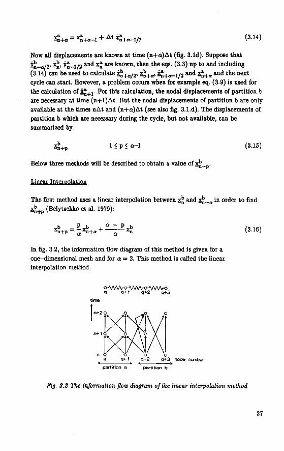
Below three methods will be described to obtain a value of ~+p·

Linear Interpolation

(3.15}

The first method uses a linear interpolation between ~~ and ~+a in order to find ~+P (Belytschko et al. 1979):

In fig. 3.2, the information flow diagram of this method is given for a one-dimensional mesh and for a = 2. This method is called the linear interpolation method.

~ q q+1 q+2 q+3

time

l n+20 0 0 0

JXI~XJ lXl~ .

n o o o o Q Q+1 q+2 q+3 node f'U'Tt)er

partition a partition b

(3.16)

Fig. 9.2 The information flow diagram of the linear interpolation method

37

Integration

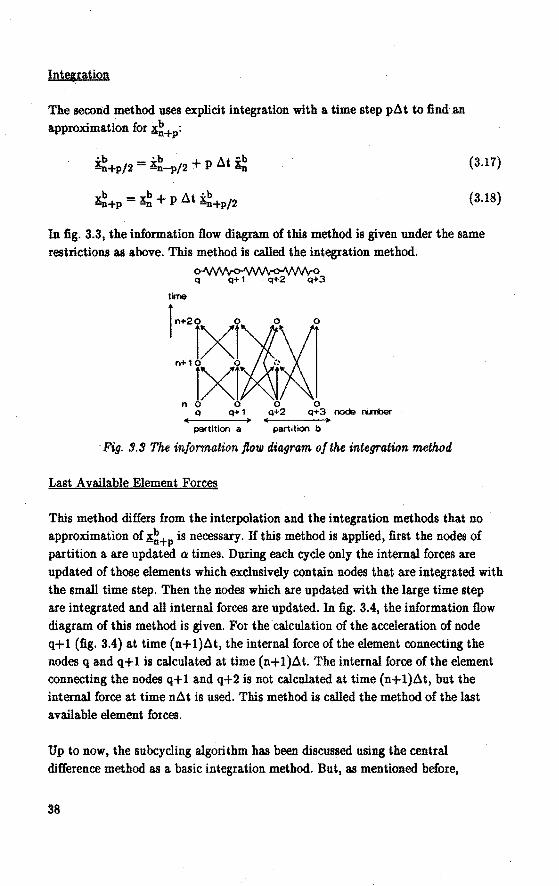
The seco:r1d method uses explicit integration with a time step pAt to findan

approximation for ~+p:

~+p/2 = ~-p/2 + p i.\t ~

~+p =~ + p i.\t ~+p/2

(3.17)

(3.18)

In fig. 3.3, the information flow diagram of this method is given under the same restrictions as above. This method is called the integration method.

~ q q+1 q+2 q+3

time l n+20 0 0 0

~·ts~fiáX n 0 0 0 0

q q+ 1 q+2 q+3 node IU'Ii:ler

partition a partition b

·Fig. 9. 9 The in formation flow diagram of the integration method

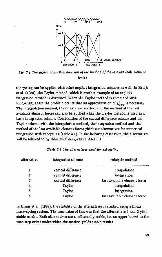
Last Ayaila.ble Element Forces

This method differs from the interpolation and the integration methods that no a.pproximation of ;JS;~+P is necessary. If this method is applied, first the nodes of partition a are npdated a times. During each cycle only the intema.l forces are npdated of those elements which exclnsively contain nodes that are integrated with the sma.ll time step. Then the nodes which are updated with the large time step are integrated and a.ll internat forces are upda.ted. In fig. 3.4, the information flow diagram of this method is given. For the calcnlation of the acceleration of node q+l (fig. 3.4) at time (n+1)i.\t, the interna.l force of the element connecting the nodes q and q+1 is calculated at time (n+l)i.\t. The intemal force of the element connecting the nodes q+l and q+2 is not calcnlated at time (n+1)6t, but the intemal force at time ni.\t is used. This method is called the method of the last available element forces.

Up to now, the subcycling algorithm has been discussed using the central difference method as a. basic integration method. But, as mentioned before,

38

~ q q+1 q+2 q+3

time

'::1~0 n o o o o

q q+1 q+2 q+3 node I"UTber

partltion 11 partitlon b

Fig. 9.4 The information flow diagram ofthe method ofthe last ava.ilable element forces

subcycling can be applied witb otber explicit integration scbemes as well. In Bruijs et al. (1988), tbe Taylor metbod, whicb is anotber example of an explicit integration metbod is discussed. When the Taylor metbod is combined with subcycling, aga.in tbe problem occurs that an approximation of ~+Pis necessary. Tbe interpolation metbod, tbe integration metbod and tbe metbod of tbe last available element forces can also be applied wben tbe Taylor metbod is used as a basic integration scbeme. Combination of the central difference scbeme and tbe Taylor scbeme witb tbe interpolation metbod, tbe integration metbod and tbe metbod of tbe last available element forces yields six alternatives for numerical integration with subcycling (table 3.1). In the following discussion, tbe alternatives will be referred to by tbeir numbers given in table 3.1

Tabk 9.1 The alternatives wed for subcycling

alternative integration scbeme subcycle metbod

1 central difference interpolation 2 . central difference integration 3 central difference last a.va.ilable element force 4 Taylor interpolation 5 Taylor integration 6 Taylor last available element force

In Bruijs et al. (1988), tbe stability of tbe alternatives is studied using a. linear mass-spring system. Tbe condusion of this was tbat tbe alternatives 1 a.nd 2 yield stabie results. Botb alternatives are conditionally sta.ble, i.e. an upper bound to tbe time step exists under whicb the metbod yields sta.ble results.

39

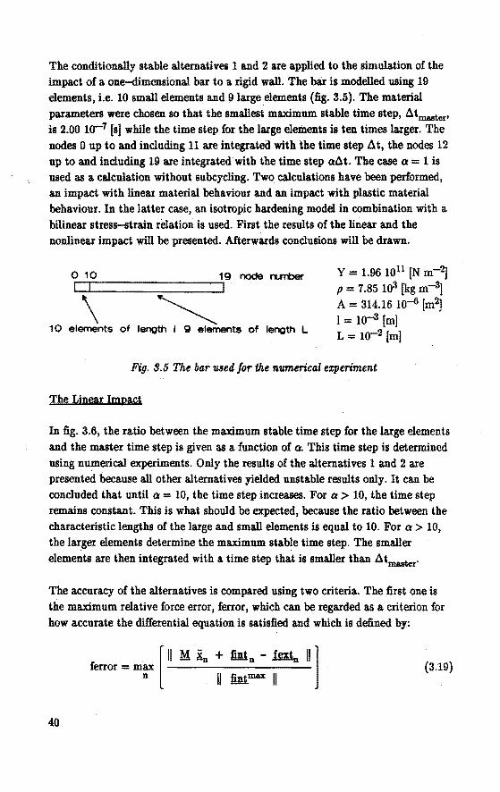
The conditionally stabie alternatives 1 a.nd 2 are applied to the simulation of the impact of a one-dimensional bar to a rigid wall. The bar is modelled using 19 elements, i.e. 10 small elements a.nd 9large elements (fig. 3.5). The material parameters were chosen so that the smallest maximum stabie time step, ~tmaster• is 2.00 w-7 [s] while the time step for the large element& is ten times larger. The nodes 0 up to a.nd including 11 are integrated with the time step ~t, the nodes 12 up to a.nd including 19 are integrated with the time step a~t. The case a= 1 is used as a calculation without subcycling. Two calculaüons have been performed, a.n impact with linear material behaviour a.nd a.n impact with plastic material behaviour. In the latter case, a.n isotropie hardening model in combination with a bilinear stress-strain relation is used. First the results of the linea.r a.nd ihe nonlinear impact will be presented. Afterwards conclusions will be drawn.

Or-1r0----------------~19 ~ ~

\ ~ 10 elements of length I 9 elements of length L

Y = 1.96 1011 [N rn-2]

p = 7.85 103 [kg m-3] A = 314.16 10-{1 [m2] 1 = 10-3 [m] L = w-2 [m]

Fig. 9.5 The bar used for the numerical experiment

The Linear Impact

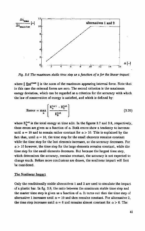
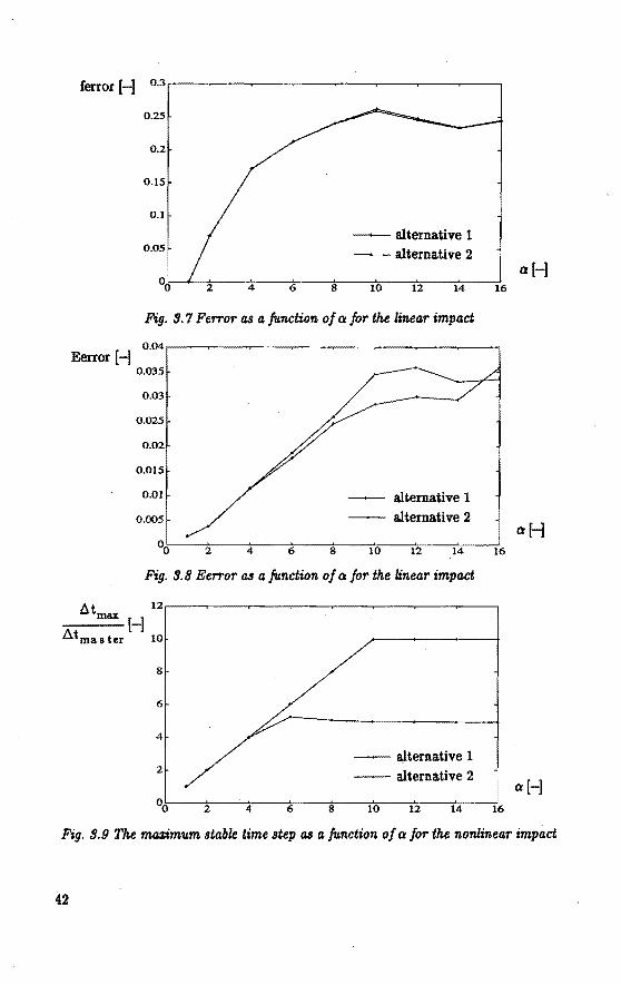
In fig. 3.6, the ratio between the maximum stabie time step for the large elements a.nd the master time step is given as a function of a. This time step is determined using numerical experiments. Only the results of the alternatives 1 a.nd 2 are presented beca.use all other alternatives yielded unstable results only. It can be concluded that until a = 10, the time step increa.ses. For a > 10, the time step remains constant. This is what should be expected, because the ratio between the characteristic lengths of the large a.nd small elements is equal to 10. For a> 10, the larger elements determine the maximum stabie time step. The smaller elements are then integrated with a time step that is smaller tha.n ~tmaster·

The accuracy of the alternatives is compared using two criteria. The first one is the maximum relative force error, ferror, which ca.n beregardedas a criterion for how accurate the differential equation is satisfied a.nd which is defined by:

[

11 M. În + fint n - fextn 11] ferror = max

n 11 fintmax 11 (3.19)

40

12r---~--~----~--~----~--~----~--,

altema.tives 1 and 2 10

8

6

4

2

a[-J

Fig. 9.6 The 11UlXim-am stable time step as a function of a for the linear impact

where 11 fintmax 11 is the norm of the maximum a.ppearing intemal force. Note that in this case the extemal forces are zero. The second criterion is the maximum energy devia.tion, which can be regarded a.s a criterion for the accuracy with which the law of conservation of energy is satisfied, and which is defined by:

(3.20)

where E!ot is the total energy at time n..:lt. In the figures 3.7 and 3.8, respectively, these errors are given a.s a function of a. Both errors show a tendency to increase until a= 10 and to rema.in rather constant for a> 10. This is expla.ined by the fa.ct that, until a = 10, the time step for the small elements rema.ins constant whiie the time step for the last elements increases, so the accura.cy decreases. For a> 10 however, the time step for the large elements rema.ins constant, whiie the time step for the small elements decreases. But because the largest time step, which deterrnines the accuracy, rema.ins constant, the a.ccuracy is not expected to change much. Before more conclusions are drawn, the nonlinear impact will first be considered.

The Nonlinear Impact

Only the conditionally stabie alternatives 1 and 2 are used to simulate the impact of a plastic bar. In fig. 3.9, the ratio between the maximum stabie time step and the master time step is given a.s a function of a. It turns out that the time step of alternative 1 increa.ses until a = 10 and then rema.ins constant. For alternative 2, the time step increa.ses until a = 6 and rema.ins almost constant for a > 6. The

41

ierror [-] 0.3,--~---.-----,.--..----.----.--~-----.

Eerror [-]

0.25

0.2

0.15

0.1

0.05 _.,...._ alternative 1 - alternative 2

Fig. 9. 7 Ferror as a fu.nction of a for the linear impact

0.04,--~-~--~-~--~-~--..----,

0.035

0.03

0.025

0.02

0.015

0.01 - alternative 1

0.005 -- alternative 2

0o~-~2~-~4--~6--~8---1~0---1~2--1~4-~16

Fig. 9.8 Eerror as a fu.nction of a for the linear impact

12.--~-~----~--~-~--~-~ 6tm.a.x -:-----[-] LHmaster 10

8

6

4

- alternative 1 2 - alternative 2

a[-]

a[-]

a[-]

Fig. 9.9 Tke mazimum stable time step as a fu.nction of a for the nonlinear impact

42

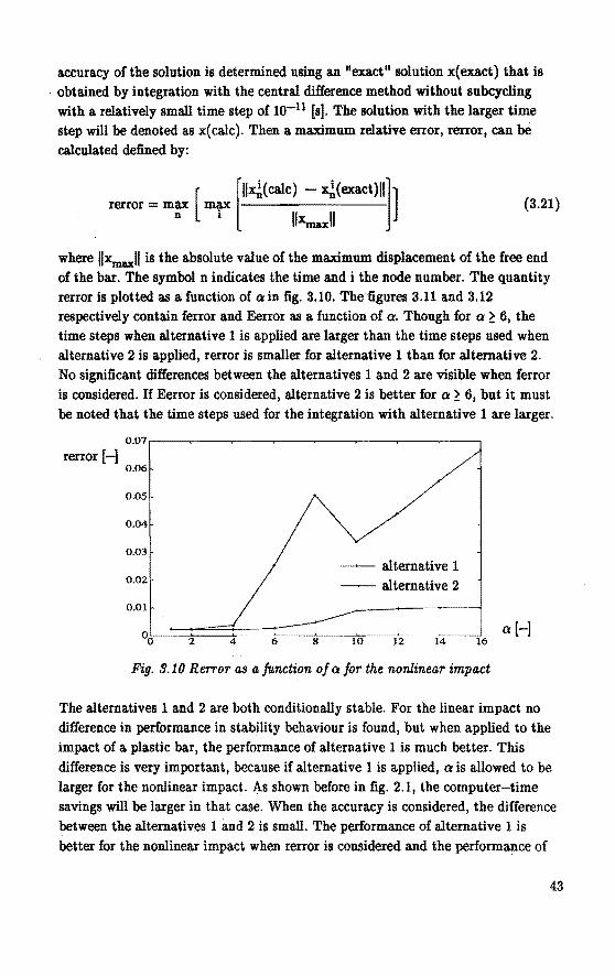
accuracy of the solution is determined using an 11exact 11 solution x( exact) that is . obtained by integration with the central difference metbod without subcycling

with a relatively small time step of w-11 [s]. The solution with the larger time step will be denoted as x( calc). Th en a maximum relative error 1 rerror 1 can bè calculated defined by:

[ [

llx!(calc) - x!(exact)II]J rerror = max max

n i ll~xll (3.21)

where 11~11 is the absolute value of the maximum displacement of the free end of the bar. The symbol n indicates the time and i the node number. The quantity rerror is plottedas a function of a in fig. 3.10. The figures 3.11 and 3.12 respectively contain ferror and Eerror as a function of a. Though for a~ 61 the time steps when alternative 1 is applied are larger than the time steps used when alternative 2 is applied, rerror is smaller for alternative 1 than for alternative 2. No significant differences between the alternatives 1 and 2 are visible when {error is considered. If Eerror is considered, alternative 2 is better for a ~ 6, but it must be noted that the time steps used for the integration withalternative 1 are larger.

rerror [-] 0.07

0.06

0.05

0.04

0.03

0.02

0.01

00 2 4 6

_,___ alternative 1

- alternative 2

10 12 14 16

Fig. 9.10 Rerror as a functi~n of a for the nonlinear impact

a[-]

The alternatives 1 and 2 are both conditionally stable. For the linear impact no difference in performance in stability behaviour is found 1 but when applied to the impact of a plastic bar, the performance of alternative 1 is much better. This difference is very important, because if alternative 1 is applied, a is allowed to be larger for the nonlinear impact. As shown before in fig. 2.1, the computer-time savings will be larger in that case. When the accuracy is considered, the difference between the alternatives 1 and 2 is smal!. The performance of alternative 1 is better for the nonlinear impact when rerror is considered and the performance of

43

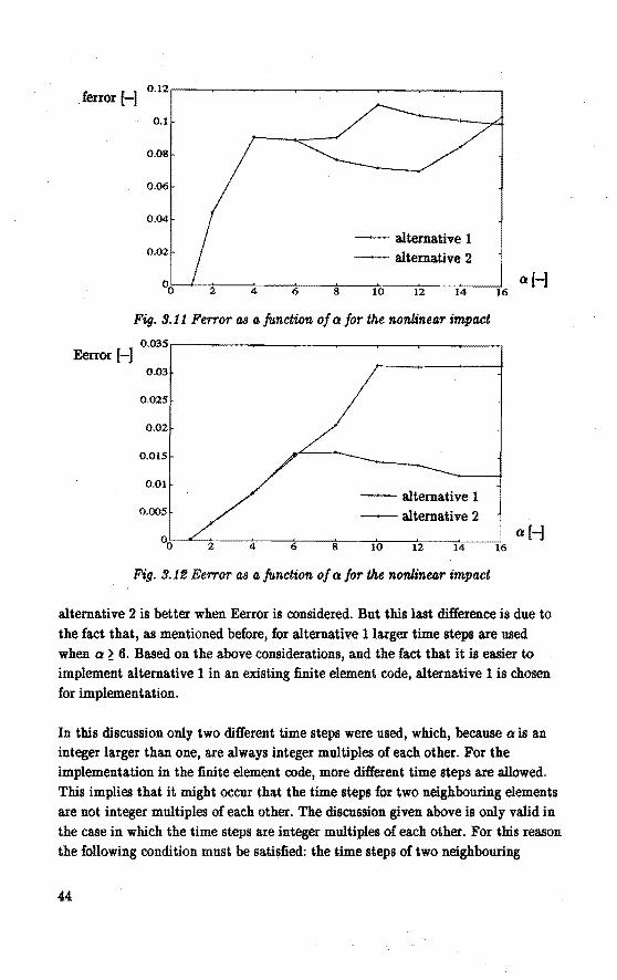
ferror [-] 0.12,--~-----.---~--~-~--~---,

0.1

0.08

0.06

0.04

-- alternative 1 0.02 -- alternative 2

Q [-]

Fig. 9.11 Ferror as a fu,nction of a for the nonlinear impact

Eerror [-] 0.005,-----~--~-~--~-~--~-~

0.03

0.025

0.02

0.015

0.01 -- alternative 1

0.005 - alternative 2

i----j4~-~6--*8----:1;';;0;-----;l;';;;2----;1':;-4---:;-'16 a[-]

Fig. 9.11! Eerror as a fu.nction of a for the nonlinear impact

alternative 2 is better when Eerror is considered. But this last di:fference is due to the fact that, as mentioned before, for alternative 1larger time steps are used when a ~ 6. Based on the above considerations, and the fact that it is easier to implement alternative 1 in an existing finite element code, alternative 1 is chosen for implementation.

In this discussion only two different time steps were used, which, because a is an integer larger than one, are always integer multiples of each other. For the implementation in the finite element code, more different time steps are allowed. This implies that it might occur that the time steps for two neighbouring elements are not integer multiples of each other. The discnssion given above is only valid in the case in which the time steps are integer multiples of each other. For this reason the following condition must be satisfied: the time steps of two neighbouring

44

elements must be integer multiples of each other.

3.3 Implem.entation in the PISCES--3DELK Program

From fig. 3.2 ·i t ca.n be seen that not every node of partition b need to be interpolated. Though a one-dimensional mesh is illustrated in fig. 3.2, it is generally true that only those nodes of partition b must be interpolated, which are connected toa finite element, which in its turn also has nodes which will be integrated with a smaller time step. This means that for an implementation of the interpolation metbod in a finite element code, the nodes must be partitioned in three groups, i.e. nodes which are updated with the small time step, nodes which are updated with the large time step and nodes which must be interpolated (though nodes which must be interpolated arealso updated with the large time step, they are only part of the last group ).

In the PISCES-3DELK code, the triangular element is put in a ra.te formulation. This means that instea.d of the nodal displacements the nodal veloeities are used for the calculation of the internat nodal forces. A linear interpola.tion of the displacements in a certain interval is the sa.me as assurning a constant velocity during that interval. In section 3.2 it is shown that the interval on which the displa.cements must be interpolated is from n.àt to (n+a).àt. On that interval the constant velocity which will yield the sa.me results as a linear interpolation is simply ~+a/2 (see eq. (3.5)). This means that no extra calculations like the interpolation are necessary for some nodes of partition b. This in turn means that the nodesneed not be divided in three groups, but that only two groups are necessary. In appendix B, theelemental calculations fora triangular constant strain membrane element in the ra.te lormulation are discussed.

The Flow Scheme for Subcycling

The flow scheme for the computations.with subcycling is given below. This scheme is divided in two parts, i.e. the generation phase and the cycler phase. The generation phase, constituted by the first six steps in the flow scheme is performed only once for a calculation. The cycler phase, constituted by the steps seven up to and including twelve, is performeq every cycle.

Start of generation phase.

1 Set initial conditions.

45

2 - Find the maximum stabie time step for ea.ch element using the Courant

criterion (2.37). - Determine the smallest time step of all maximum stabie time steps: fltmaster· - Pa.rtition the elements in groups. Ea.ch group conta.ins elements that will he

integrated with a time step aàtmaater, where a is a positive integer. An element will be part of that group with the la.rgest a satisfying

aàtmaster ~ Mma.x, where fltma.x is the maximum stabie time step for the element.

3 H an element is a neighbour of one or more elements with a smaller a, the element will he part of the group with the smallest a of all neighbours.

4 Find the combination of a's, satisfying the condition tha.t ea.ch a is a. divisor of alllarger a's, requiring the smallest number of element ca.lculations. This yields

the group partition tha.t will he used for the ca.lculation. Let a1e be the a of element group I.

5 Split the nodes in groups with equa.l a. The a of a node is equa.l to the

maximum a of all connected elements. Let ~P be the a of node group I.

6 Initia.lize the clocks:

- tmaater = 0 set the master time to zero;

- tie= 0 - tip= 0

set the element group time to zero;

set the noda.l group time to zero.

End of the generation pha.se.

Start of the cycler pha.se.

7 Increase the master time:

tmaster = tmaster + à tmaster

8 Loop over all node groups

IF t1P < tmuter THEN

46

- Set the time step for allnodesin group I to a1P fltmaster·

- Update the group time: t1P = t1P + a1P fltmaster· ELSE

- Set the time steps for a.ll nodes in group I to zero. ENDIF

End loop over a.ll node groups.

9 Caleula.te the a.ccelera.tions of the nodes a.nd update the veloeities using the central difference metbod with the time step determined in step 8. Update the

displacements with .1-tiiJallter

10 Loop over all element groups

IF tinallter - tie = ale 6 tinallter THEN Loop over allelementsin group I - Calcula.te the strain rates

- Calcula.te the stress rates - Calculate the new stresses - Calculate the nodal internal forces

End loop over all elements in group I Update the element group time: tie= tie+ a1e6tiiJallter

ELSE Skip group I

ENDIF End loop over all element groups.

11 Determine the extemal nodal forces.

12 Go to 7

End cycler pha.se.

Some of the steps in the algorithm need some extra comments. This is done below

for the steps 3, 5, 8 a.nd 10. Step 4 is discussed more extensively in section 3.4.

H an element is a neighbour of an element with a smaller a, this mea.ns that this element ha.s nodes which must be integrated with a smaller time step. This implies

that the internal forcesof the element must be updated with the smaller time step. That is the rea.son why an element which has neighbours which are integrated with

a smaller time step, must be part of the group with the smallest time step of all

neighbours.

Because in step 3 the elements which are neighbours of one or more elements with

a smaller a become a p.art of the group with the smallest a, the time, step with

47

which a node can he integrated is now equat to the largest time step of all elements

connected to that node.

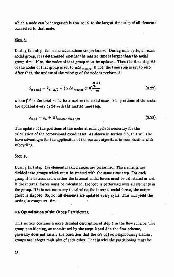
During this step, the nodat calculations are performed. During each cycle, for each nodat group, it is determined whether the master time is larger than the nodal group time. If so, the nodesof that group mnst be updated. Then the time step at

of the nodesof that group is set to aatmaater· If not, the time step is set to zero. After that, the update of the velocity of the node is performed:

f! ot

in+a/2 = in.-a/2 +(a atmaater or 0>-=m- (3.22)

where fot is the totat nodal force and m the nodat mass. The positions of the nodes are updated every cycle with the master time step:

(3.23)

The update of the positions of the nodes at each cycle is necessary for the calculation of the corota.tionat coordinates. As shown in section 3.6, this will also have advantages for the application of the contact atgorithm in combination with subcycling.

Step 10.

During this step, the elemental calculations are performed. The elements are divided into groups which must he treated with the same time step. For each

group it is determined whether the internal nodal forces must be calculated or not. If the internat forces must he catculated, the loop is performed over all elements in the group. If it is not necessary to calculate the internat nodat forces, the entire group is skipped. So, notall elements are updated every cycle. This will yield the saving in computer-time.

3.4 Optimization of the Group Partitioning.

This section contains a more detailed description of step 4 in the fiow scheme. The group partitioning, as constituted by the steps 2 and 3 in the fiow scheme, generally does not satisfy the condition that the a's of two neighbouring element

groups are integer multiples of each other. That is why the partitioning must be

48

changed. In this section an algorithm is described which automatically finds that · group division, satisfying the condition mentioned above and yielding the largest computer-time savings. This implies that the user doesnothave to bother about the partitioning.

Let the elements he divided into groups according to the steps 2 and 3 of the flow scheme. Let the number of element groups he equal to ~t· Let the time step ratio of group I he equal to a1 and the number of elements in group I he n1. Let the simwation time he TBi.m and the smallest time step àtmaater· Let k he the costs per element-cycle. Then the total costs K are equal to:

nt ot ni T sim K= I: ---k

1=1 ~ At (3.24)

The costs calculated with (3.24) are the absolute minimum which can he achieved wiih subcycling, but this absolute minimum is not always allowed. The a's of two neighbouring element groups must he integer multiples of each other. Because it is too costly to check whether this condition is satisfied, only combinations of a

which are all integer multiples of ea.ch othèr are checked. The subroutine OPTIMIZE finds the combination of allowable a's for which the costs are minimal. First all allowable combinations of a are determined. Then for each combination of a the number of element groups and the numher of elements per group are determined. (Note that an element which is originally in a group with e.g. a = 4 can also he placed in a group with a smaller a.) Then the costs are calculated using (3.24) with the new numher of groups and numher of elements per group. The combination of a's with the minimum costs is saved and used for the calculations.

Remarks: 1 The costs as calculated with (3.24) arebasedon the assumption that all

calculations during a cycle are subcycled. This is not true, so the real costs will always he higher than calculated with (3.24).

2 As mentioned before, the claim that all a's must he integer multiples of each other is too strict. In fact only the a's of two neighbouring groups must he integer multiples of each other. Application of OPTIMIZE tothetest examples showed tha.t the saving in the computer-time with ihe too strict claim does not differ much from the maximum attainable savings. Tha.t is why the too strict claim is maintained in the a.lgorithm.

49

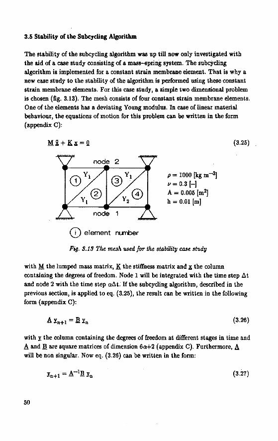
3.5 Stability of the Subcycling Algorithm.

The sta.bili~y of the subcycling algorithm was up till now only investiga.ted with the a.id of a. case study consisting of a. mass-t~pring system. The subcycling algorithm is implemented for a. constant stra.in membrane element. That is why a new case study to the stability of the algorithm is performed using these constant stra.in membrane elements. For this case study, a simple two dimensional problem is chosen (fig. 3.13). The mesh consists of four constant strain membrane elements. One of the elements has a. deviating Young modulus. In case of linear material beha.viour, the equations of motion for this problem can be wntten in the form (appendix C):

(D element nunber

p = 1000 [kg m-3J 11 = 0.3 [-]

A = 0.005 [m2] h = 0.01 [m]

Fig. 9.19 The mesh used for the stability casestudy

(3.25)

with M the lumped mass matrix, K the stiffness matrix a.nd ~ the column conta.ining the degrees of freedom. Node 1 will be integrated with the time step Llt and node 2 with the time step allt; If the subcycling algorithm, described in the previous section, is a.pplied to eq. (3.25), the result can be wriUen in the following form (appendix C):

(3.26)

with I the column conta.ining the degrees of freedom at different stages in time and A and!! are square matrices of dimension 6a+2 (appendix C). Furthermore, A will be non singular. Now eq. (3.26) can be written in the form:

(3.27)

50

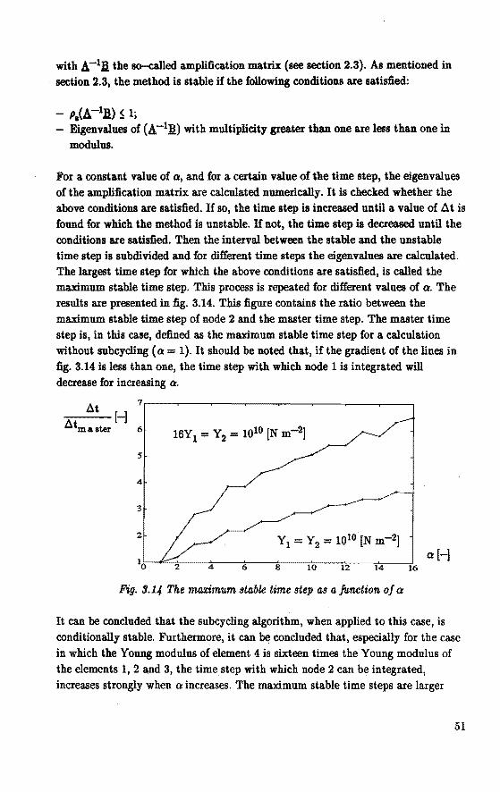
with A.-111 the so-called amplification matrix (see section 2.3). As mentioned in

section 2.3, the metbod is stabie if the following conditions are satisfied:

- P1(A.-111) S 1; - Eigenvalnes of (A. - 111) with multiplicity greater than one are Iess than one in

modulus.

For a constant value of a, and for a certain value of the time step, the eigenvalnes

of the amplification matrix are calculated numerically. It is checked whether the

above conditions are sa.tisfied. If so, the time step is increased until a value of .ó.t is

found for which the metbod is unstable. If not, the üme step is decreased until the

conditions are satisfied. Then the interval between the stabie and the unstabie time step is subdivided and for different time steps the eigenvalnes are calculated. The Iargest time step for which the above conditions are satisfied, is called the maximum stabie time step. This process is repeated for different values of a. The

results are presented in fig. 3.14. This ligure contains the ratio between the maximum stabie üme step of node 2 and the master time step. The master time

step is, in this case, defined as the maximum stabie time step for a calculation

without subcycling (a = 1 ). It should be noted that, if the gradient of the lines in fig. 3.14 is Iess than one, the time step with which node 1 is integra.ted will

decrea.se for increasing a.

7.---~--~----~--~--~----~--~---, At [-]

.ó.tm a ster 6

s

4

a[-]

Fig. 9.1-t The maximum stable time step as a fu,nction of a

It can be concluded that the subcycling algorithm, when applied to this case, is

conditionally stable. Furthermore, it ca.n be concluded tha.t, especially for the case

in which the Young modulus of element 4 is sixteen times the Young modulus of

the elements 1, 2 and 3, the time step with which node 2 can be integrated,

increases strongly when a: increases. The maximum stabie time steps are larger

51

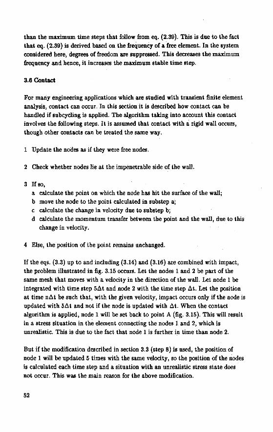
than the ma.:x:imum time steps that follow from eq. (2.39). This is due tothefact that eq. (2.39) is derived based on the frequency of a free element. In the system considered here, degrees of freedom are suppressed. This decreases the ma.:x:imum frequency and hence, it increases the ma.:x:imum stable time step.

3.6 Contact.

For many engineering applications which are studied with transient finite element

analysis, contact can occur. In this section it is described how contact can be handled if subcycling is applied. The algorithm taking into account this contact involves the following steps. It is assumed that contact with a rigid wall occurs, though other contactscan be treated the same way.

1 Updatethenodes as if they were free nodes.

2 Check whether nodes lie at the impénetrable si de of the wall.

3 If so, a calculate the point on which the node has hit the surface of the wall; b move the node to the point calculated in substep a; c calculate the change in velocity due to substep b; d calculate the momenturn transfer between the point and the wall, due to this

change in velocity.

4 Else, the position of the point remains unchanged.

If the eqs. {3.3) up to and including (3.14) and (3.16) are combined with impact, the problem illustrated in fig. 3.15 occurs. Let the nodes 1 and 2 be part of the same mesh that moves with a velocity in the direction of the wall. Let node 1 be integrated with time step 56t and node 2 with the time step 6t. Let the position at time n6t be such that, with the given velocity, impact occurs only if the node is updated with 56t and not if the node is updated with at. When the contact algorithm is applied, node 1 will be set back to point A (fig. 3.15). This will result in a stress situation in the element connecting the nodes 1 and 2, which is unrealistic. This is due to the fact that node 1 is further in time than node 2.

But if the modiBeation described insection 3.3 (step 8) is used, the position of node 1 will be updated 5 times with the same velocity, so the position of the nodes

is calculated each time step and a situation with an unrealistic stress state does not occur. This was the main reason for the above modification.

52

wan

Fig. 3.15 Interaction with a waU

The same strategy is used for interaction with ellipsoids instead of walls. A contact algorithm taking into account mutual contacts between the elements, can also be treated as mentioned above to make the algorithm combinable with subcycling.

3. 7 Test Examples

In this section, the subcycling algorithm is applied to a number of test examples. All test examples are also simulated using a calculation without subcycling, so the results of a calculation with subcycling can be compared with the results of a calculation without subcycling. In the first test example, the plàte, it is tested whether many time steps and whether large time step ratio's are allowed. External forces are absent and the plate will remain in its pla.ne. In the second test example, the membra.ne under pressure, the membrane is loaded with an external pressure perpendicular to the plane of the membrane. This test example is done to study the behaviour of subcycling in combination with externalloads. The third test example, the membrane impacting with a wall, is used to verify contact with a rigid wall in combination with subcycling. The fourth test example, the membrane impacting with the ellipsoid, is used to test the interaction with ellipsoids in combination with subcycling. It is remarked that these test examples are used for the testing of the subcycling algorithm and not to show that subcycling yields large computer-time savings. For some of the test examples, the computer-time savings are negligible, but that is what can be expected basedon the discussion in section 2.6. Inthelast test example, the simulation of the inflation of a driver si de airbag with exhaust orifices, it is shown that subcycling does yield substa.ntial computer-time savings for practical problems.

53

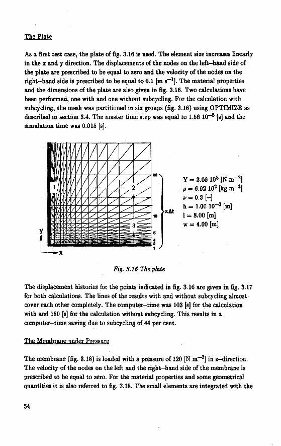
The Plate

As a first test case, the plate of fig. 3.16 is used. The element size increases linearly in the x and y direction. The displacements of the nodes on the left-hand side of the plate are prescribed to be equal to zero and the velocity of the nodes on the right-hand side is prescribed to be equal to 0.1 [m s-1]. The material properties and the dimensions of the plate are &lso given in fig. 3.16. Two calculations have been performed, one with and one without subcycling. For the calculation with subcycling, the mesh was partitioned in six groups (fig. 3.16) using OPTIMIZE as described insection 3.4. Themaster time step was equal to 1.56 10-s [s] and the simulation time was 0.015 [s].

Fig. 3.16 The plate

Y = 3.06 108 [N m-2]

p = 6.92102 [kg m-3] v=0.3 [-] h = 1.00 10-3 [m] 1 = 8.00 [m} w = 4.00 (m)

The displacement histories for the points indicated in fig. 3.16 are given in fig. 3.17 for both calculations. The lines of the results withand without subcycling almost cover each other completely. The computer-time was 103 [s] for the calculation withand 180 (s] for the calculation without subcycling. This results in a computer-time saving due to subcycling of 44 per cent.

The Membrane under Pressure

The membrane (fig. 3.18) is loaded with a pressure of 120 [N m-2] in z-direction. The velocity of the nodes on the left and the right-hand side of the membrane is prescribed to be equal to zero. For the material properties and some geometrical quantities it is also referred to fig. 3.18. The small elements are integrated with the

54

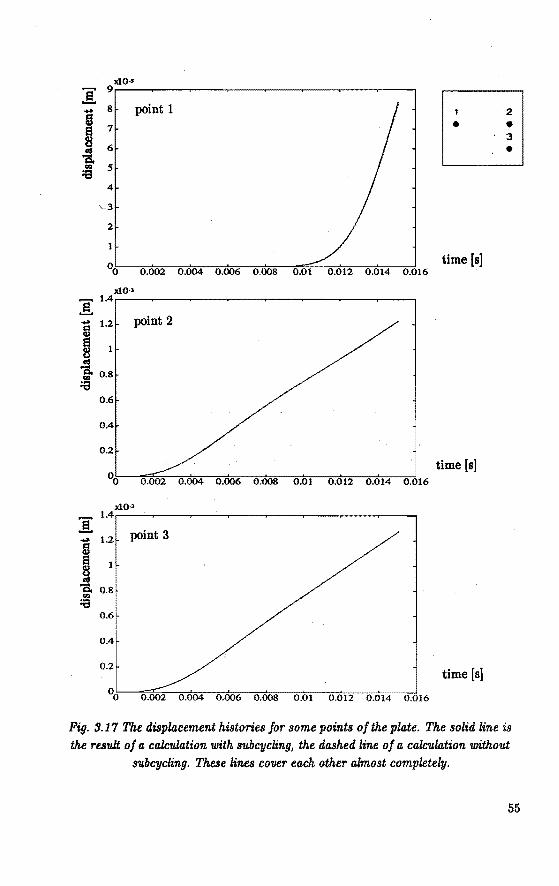
xlO ..

A 9

.... 8 point 1 2

I 7 • • 3

-ä 6 • ... 5 :a 4

'-3

2

1

00 time [s]

0.002 0.004 0.006 0.008 O.ol

xlO-> A 1.4

.... 1.2 point 2

I -a. ... 0.8 :a

0.6

0.4

0.2

00 time (s]

O.ot 0.012 0.014 0.016

xl0-3

A 1.4

point 3 .... 1.2 §3

! ]. 0.8

:a 0.6

0.4

0.2 time [s]

00 0.002 0.004 0.006 0.008 0.01 0.012 0.014 0.016

Fig. 9.11 The displacement historiesforsome points ofthe plate. The solid line is the result of a calculation with subcycling, the dashed line of a cablation without

subcycling. These lines cover each other almost completely.

55

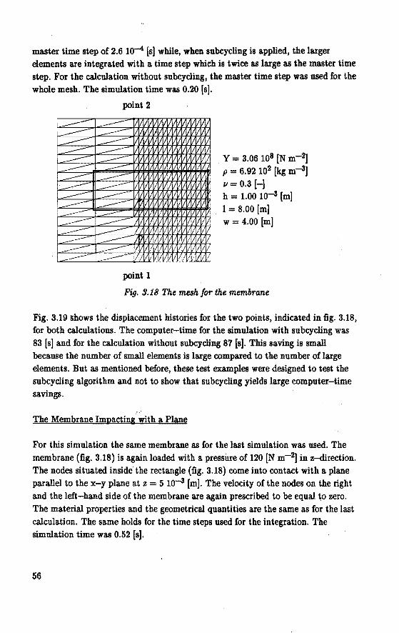
master time step of 2.6 10-4 [s] while, when subcycling is applied, the larger elements are integrated with a time step which is twice as large asthemaster time step. For the calculation without subcycling, the master time step was used for the whole mesh. The simulation time was 0.20 [s].

point 2

point 1

Y = 3.06 108 [N m-2]

p = 6.92 102 [kg m-3]

v = o.3 H h = 1.00 10-3 [m]

1 = 8.00 [m] w = 4.00 [m]

Fig. 3.18 The mesh for the membrane

Fig. 3.19 llhows the displacement histories for the two points, indicated in fig. 3.18,

for both calculations. The computer-time for the simulation with subcycling was 83 [s] and for the calculation without subcycling 87 [s]. This saving is small because the number of small elements is large compared to the number of large elements. But as mentioned before, these test examples were designed totest the subcycling algorithm and not to show that subcycling yields large computer-time savings.

The Membrane Imnaçting with a Plane

For this simulation the same membrane as for the last simulation was used. The membrane (fig. 3.18) is again loaded with a pressure of 120 [N m-2] in z--direction. The nodes situated inside the rectangle (fig. 3.18) come into contact with a plane parallel to the x-y plane at z = 5 10-3 [m]. The velocity of the nodes on the right and the left-hand si de of the membrane are again prescribed to be equal to zero. The material properties and the geometrical quantities are the same as for the last calculation. The same holds for the time steps used for the integration. The simulation time was 0.52 [s].

56

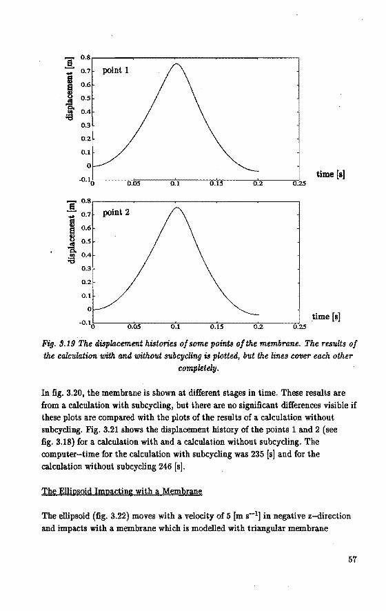
A 0.8

i 0.7 point 1

B 0.6

0.5 ct -a 0.4 GQ :a 0.3

0.2

0.1

-0.10 0.05 0.1 0.15 time [s]

A o.8

point 2 i

0.7

a 0.6

8 0.5 ct -a :ä 0.4

0.3

0.2

0.1

-0.10 0.05 0.1 0.15

_time [s]

Fig. 3.19 The displacement histories of some points ofthe membrane. The results of the calculation with and without subcycling is plotted, but the lines cover each other

completely.

In fig. 3.20, the membrane is shown at different stages in time. These results are from a calculation with subcycling, but there are no significant differences visible if these plots are compared with the plots of the results of a calculation without subcycling. Fig. 3.21 shows the displacement history of the points 1 and 2 (see fig. 3.18) for a calculation with and a calculation without subcycling. The computer-time for the calculation with subcycling was 235 [s] and for the calculation without subcycling 246 [s].

The Ellipsoid lmpacting with a Membrane

The ellipsoid (fig. 3.22) moves with a velocity of 5 [m s-1] in negative z-direction and impacts with a membrane which is modelled with triangular membrane

57

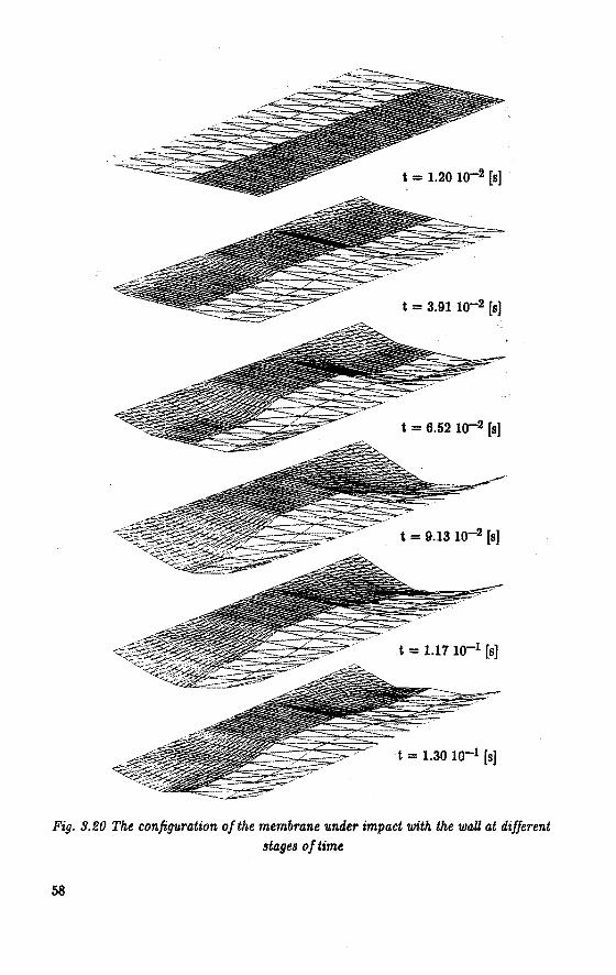
t = 1.20 10-2 [s]

t = 3.911o-2 [s]

t = 1.30 w-1 [s]

Fig. 9.20 The configuration of the membrane under impact with the wallat different stages of time

58

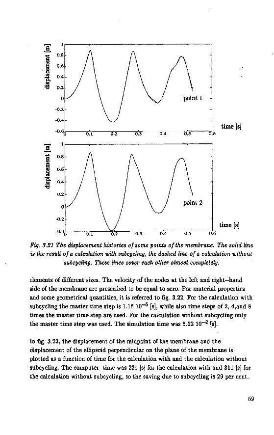
Fig. 9.21 The displacement histories of some points ofthe membrane. The solid line is the result of a calculation with subcycling, the dashed line of a calculation without

subcycling. These lines cover each other almost completely.

elements of different sizes. The velocity of the nodes a.t the left a.nd right-ha.nd

side of the membra.ne are prescribed to be equal to zero. For material properties

a.nd some geometrical quantities, it is referred to fig. 3.22. For the calculation with

subcycling themaster time step is 1.16 10-5 [s], while also time steps of 2, 4,and 8

timesthemaster time step are used. For the calcula.tion without subcycling only

themaster time step was used. The simula.tion time was 5.22 w-2 [s].

In fig. 3.23, the displacement of the midpoint of the membra.ne a.nd the displacement of the ellipsoid perpendicula.r on the pla.ne of the membra.ne is

plotted as a tunetion of time for the calculation with and the calculation without

subcycling. The computer-time was 221 [s] for the calculation with a.nd 311 [s) for

the calculation without subcycling, so the saving due to subcycling is 29 per cent.

59

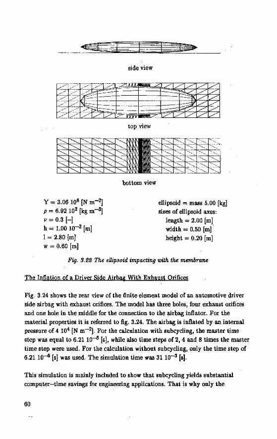
---~+& f 4t

Y = 3.06 108 [N m-2] p = 6.92 102 [kg m-3] v=0.3 [-] h = 1.00 10-2 [m] 1 = 2.80 [mJ w = 0.60 [m]

side view

top view

bottomview

ellipsoid = mass 5.00 [kg] sizes of ellipsoid axes:

length = 2.00 [m] width = 0.50 [m] ·

height = 0.20 [m]

Fig. 9.22 The ellipsoid impacting with the membrane

The Inflation of a Driver Side Airbag With Exhaust Orifices

Fig. 3.24 shows the rear view of the fini te element model of an automotive driver side airbag with exhaust orifices. The model has three holes, four exhaust orifices and one hole in the middle for the conneetion to the airbag inflator. For the material properties it is relerred to fig. 3.24. The airbag is inflated by an internal pressure of 4 104 [N m-2]. For the calculation with subcycling, themaster time step was equal to 6.2110-6 [s], while also time steps of 2, 4 and 8 timesthemaster time step were used. For the calculation without subcycling, only the time step of 6.2110-6 [s] was used. The simulation time was 3110-3 [s].

This simulation is mainly included to show that subcycling yields substantial computer-time savings for engineering applications. Tha.t is why only the

60

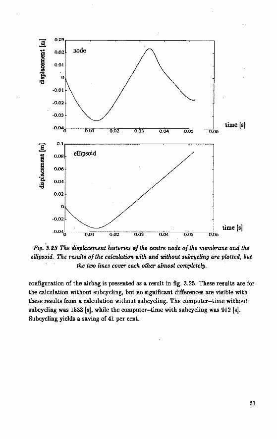
]: 0.03

i 0.02 node

I 0.01

13. 0 re :a

·0 ·04o:,-----"o~.o"t-~o..-.o~2.---;;o:-:;_o"'3--o".~04.---,o~.o"'s--.,.-!o.06 time [s]

0.1.-----~--~---....---~--~---,

0.08 ellipsoid

0.06

0.04

0.02

0

time [s] 0.04 0.05 0.06

Fig. 9.29 The displacement histories of the centre node of the membrane and the eUipsoid. The results of the calculation with and without subcycling are plotted, but

the two linea cover each other almost completely.

configuration of the airbag is presented as a result in fig. 3.25. These results are for the calculation without subcycling, but no significant differences are visible with these results from a calculation without subcycling. The computer-time without

snbcycling was 1533 [s], while the computer-time with subcycling was 912 [sJ. Snbcycling yields a saving of 41 per cent.

61

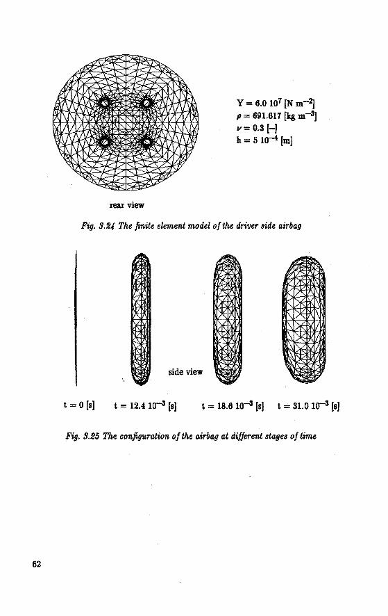
62

rear view

Y = 6.0 107 [N m-2] p = 691.617 [kg m-3] u=0.3 (-] h = 51o-4 [m]

Fig. 3.2./ The finite element model ofthe driver side airbag

side view

t = 0 [s] i = 12.4 10-3 (s] t = 18.6 1o-3 [s] t = 31.0 1o-3 [sJ

Fig. 3.25 The configuration ofthe airbag at different stages of time

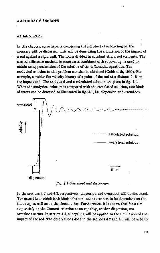
4 ACCURACY ASPECTS

4.11ntroductioa

In this chapter, some aspects concerning the infiuence of subcycling on the accuracy will be discussed. This wiii be done Using tbe simwation of tbe impact of

a rod a.gainst a. rigid wall. Tbe rod is divided in constant strain rod elements. Tbe

central difference metbod, in some cases combined witb subcycling, is used to

obtain an a.pproxima.tion of tbe solution of the differentia.l equations. Tbe ana.lytica.l solution to this problem can a.lso be obtained (Goldsmitb, 1960). For exa.mple, consider tbe velocity history of a. point of tbe rod at a. dista.nce 11 from

tbe impact end. Tbe a.nalytical a.nd a. ca.lcula.ted solution are given in fig. 4.1. When tbe a.nalytical solution is compa.red witb tbe calcula.ted solution, two kinds

of errors ca.n be detected as illustra.ted in fig. 4.1, i.e. dispersion a.nd oversboot.

oversboot

: I I

! I

•' :\ ; \ ; \ f\ /\

I i

I --------- ca.lculated solution j

a.na.lytica.l solution

time

dispersion

Fig. -f.1 Overskoot and dispersion

In the sections 4.2 a.nd 4.3, respectively, dispersion a.nd oversboot will be discussed.

The extent into which botb kinds of errors occur turns out to be dependent on the

time step as wen as on tbe element size. Furtbermore, it is sbown tbat for a time

step satisfying tbe Courant criterion as a.n equa.lity, neitber dispersion, nor

oversboot occurs. In section 4.4, subcycling will be applied to the simula.tion of the

impact of tbe rod. The observations done in the sections 4.2 and 4.3 will be used to

63

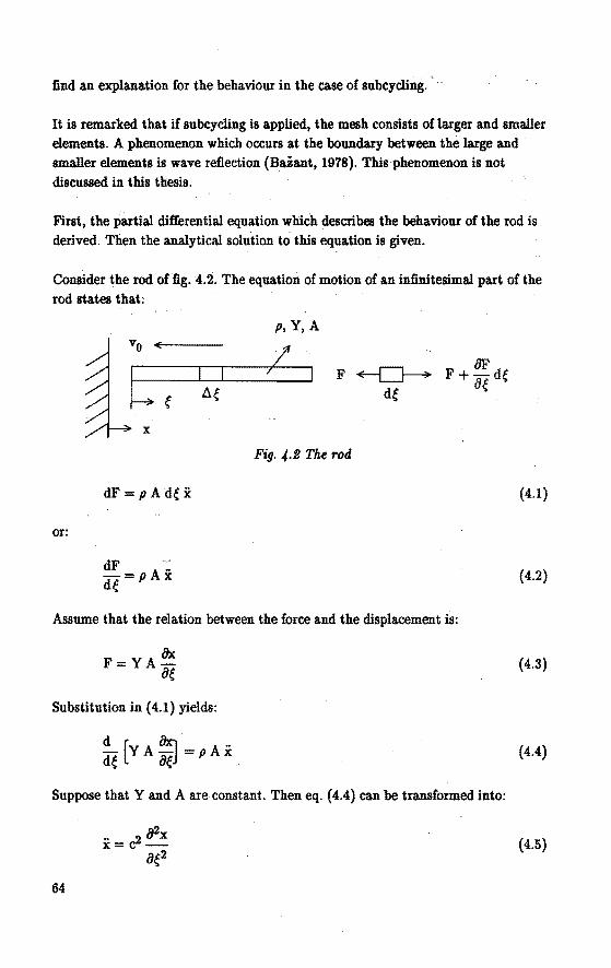
find an explanation for the behaviour in the case of subcycl.ing.

It is remarked that if subcycl.ing is applied, the mesh consists of larger and smaller elements. A phenomenon which occurs at the boundary between the large and · smaller elements is wave reflection (Baiant, 1978). This phenomenon is not discussed in this thesis.

First, the partial differential equation which describes the behaviour of the rod is derived. Then the analytica! solution to this equation is given.

Consider the rod offig. 4.2. The equation of motion of an infinitesimal part of the rod states that:

or:

x

dF =PA de x

dF A_ -=p x de

p, Y, A

I I 7 I

Fig. 4.2 The rod

Assume that the relation between the force and the displacement is:

fJx F=YA­ae

Substitution in (4.1) yields:

Suppose that Y and A are constant. Then eq. (4.4) can he transformed into:

64

(4.1)

(4.2)

(4.3)

(4.4)

(4.5)

wit à:

' y il=­

p

The general form of the analytical salution of eq. { 4.5) is:

x(~,t) = f(~ -ct)+ g(e +ct)

(4.6)

(4.7)

This can easily be verified by substitution of ( 4.7) in ( 4.5). The functions f and g

repreaent waves that move with a velocity c in respectively the positive and negative e-mrection. The sàape of the functions f and g is determined from the

initial and boundary conditions. The quantity c is the wave propa.gation speed.

4.2 Dispenion

Dispersion can be defined as the change of the wave propagation speed due to

spatial and/or time discretization. Herea.fter, the influence of spatial discretization,

time discretization and the influence of both spatial and time discretization on the wave propagation speed will be studied.

Spatial Discretization

Suppose that the spatial discretization is performed using a central difference method:

where tbe subscript m indicates the node number and ae the element size. Substitution of ( 4.8) in ( 4.5) yields

Assume that the solution is of the form:

{4.8)

(4.9)

{4.10)

with A the complex amplitude, w the angular frequency and w8

the spatial

frequency whicb is related to the wave length ..\. according to:

65

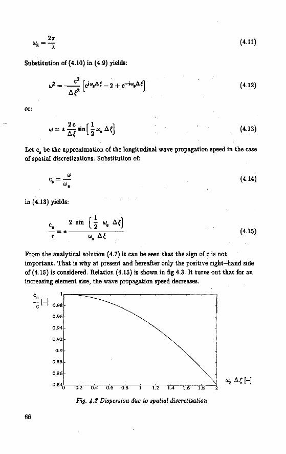
(4.11)

Substitution of (4.10) in (4.9) yields:

(4.12)

or:

w=:~:!:sin(~w fl.t] ll.e 2 s "' (4.13)

Let c8

be the approximation of the longitudinal wave propaga.tion speed in the case

of spa.tial discretizations. Substitution of:

(4.14)

in (4.13) yields:

(4.15)

From the a.nalytical salution ( 4. 7) it can be seen that the sign of c is not

important. That is why a.t present and herealter only the positive right-ha.nd side of (4.15) is considered. Rela.tion (4.15) is shown in :fig 4.3. lt turns out that for a.n

increasing element size, the wave propagation speed decrea.ses.

Cs -eH 0.98

0.96

0.94

0.92

0.9

0.88

0.86

0•84o 0.2 0.4 0.6 0.8 1.2 1.4 1.6 1.8 2

Fig. 4.9 Dispersion due to spatial discretization

66

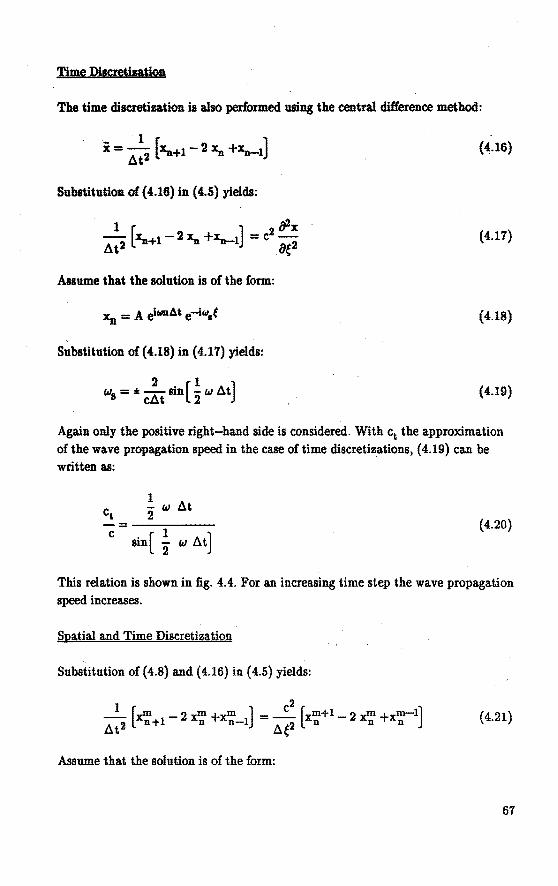
Time Discreüzaüon

The time discretization is also performed using the central difference meihod:

1 x = - [Xa+l - 2 x. +z.-t] At2

Subsiiiuiion of (4.16) in (4.5) yields:

Assume that the solution is of the form:

Substitution of (4.18) in (4.17) yields:

"'s = :1: ....!_sin(!. wAt] cAt 2

(4.16)

(4.17)

(4.18)

(4.19)

Again only the positive right-hand si de is considered. With ct the approximation of the wave propagaiion speed in the case of time discretizations, ( 4.19) can be written as:

1 - w At 2

-=--:----c sin( ~ w At]

(4.20)

This relation is shown in fig. 4.4. For an increasing time step the wave propagation speed increases.

Spatial and Time Discretization

Substitution of ( 4.8) and ( 4.16) in ( 4.5) yields:

(4.21)

Assume that the solution is of the form:

67

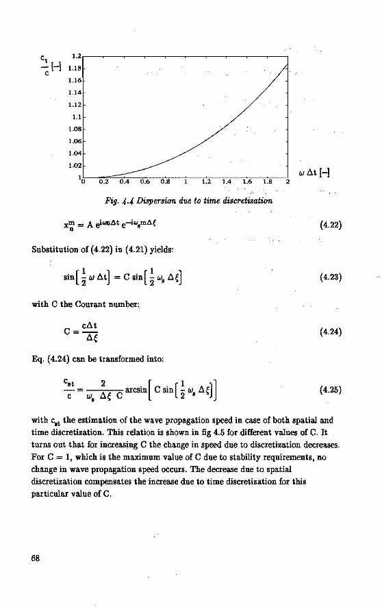
ct 1.2

-{-] 1.18 c

1.16

1.14

1.12

1.1

1.08

1.06

1.04

1.02

10 wAt[-]

0.2 1.6 1.8 2

Fig. 4.4 Dispersion due to time discretization

(4.22)

Substitution of (4.22) in (4.21) yields:

sin[~ w 8t] = C sin[~ w8 8~] (4.23)

with C the Courant number:.

(4.24)

Eq. (4.24) can be transformed into:

(4.25)

with est the estimation of the wave propa.gation speed in case of both spatial and time discretization. This relation is shown in fig 4.5 for different valnes of C. It turns out that for increa.sjng C the change in speed due to discretization decrea.ses. For C = 1, which is the maximum value of C due to stability requirements, no change in wave propagation speed occurs. The decrea.se due to spatial discretization compensates the încrea.se due to time discretization for this pa.rticular value of C.

68

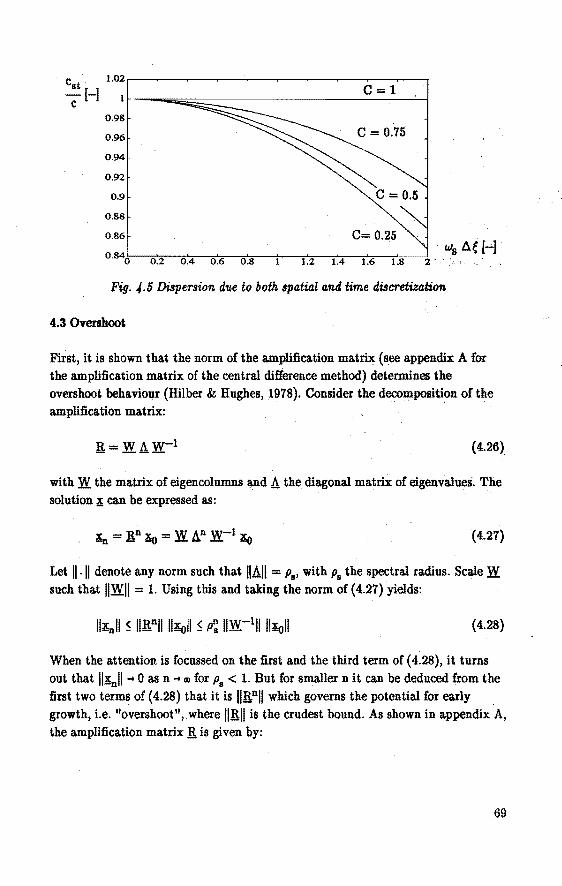
0.98

0.96

0.94

0.92

0.9

0.88

0.86

0 •84o 0.2 0.4 0.6 0.8 1.2 1.4 1.6 1.8 2 ·.

Fig. ,f.5 Dispersion d'Ue to both spatial and time discretization

4.3 Oversboot

First, it is shown that the norm of the a.mplification matrix (see appendix A for the a.mplification matrix of the central difference method) determines the oversboot behavioijr (Hilber & Hughes, 1978). Consider the decomposition of the a.mplification matrix:

. (4.26)

with W the matrix of eigencolumns and A the diagonal matrix of eigenvalues. The solution J; can be expressed as:

(4.2'7)

Let 11·11 denote any norm such that IIAII = p8 , with p8 the speetral radius. Scale W such that IIWII = 1. Using this and taking the norm of ( 4.27) yields:

(4.28)

When the attention is focussed on the first and the third term of (4.28), it turns out that 11~11 -. 0 as n -. m for p

8 < 1. But for smaller n it can be deduced from the

first two termsof (4.28) that it is IIRnll which governs the potential for early

growth, i.e. "overshoot", where IIRII is the crudest bound. As shown in appendix A, the a.mplification matrix Ris given by:

69

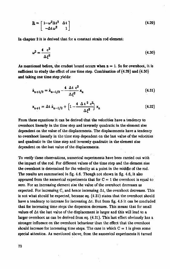
(4.29}

In chapter 2 it is derived that for a constant strain rod element:

(4.30)

As meniioned before, the crudest bound oceurs when n = 1. So for overshoot, it is sufficient to study the effect of one time step. Combination of (4.29) a.nd (4.30)

a.nd taking one time step yields:

(4.31)

(4.32)

From these equations it ea.n be derived that the veloeities have a tendency to oversboot linearly in the time step a.nd inversely quadratic in the element size dependent on the value of the displacements. The displacements have a tendency to overshooi linearly in the time step dependent on the last value of the veloeities a.nd quadratic in the time step and inversely quadratie in the element size dependent on the last value of the displacements.

To verify these observations, numerical experiment& have been earried out with the impact of the rod. For different values of tbe time step and the element size the oversboot is determined for the velocity at a point in the midd!e of the rod. The results are summarized in fig. 4.6. Though not shown in fig. 4.6, it also

appeared from the numerical experiments that for C = 1 the oversboot is equal to zero. For an increasing element size tbe value of tbe oversboot decreases as expected. For increasing C, and bence increasing At, tbe oversboot decreases. This is not wbat should he expected, because eq. (4.31) statestbat the oversboot should have a tendency to inerease for increasing At. But from fig. 4.5 it ean he eoncluded that for increasi~g time steps the dispersion decreases. This means that for small values of At the last value of tbe displacement is larger and this willlead to a largeroversboot as can be derived from eq. (4.31). This last effect obviously bas a stronger influence on the oversboot behaviour than the effect that the oversboot sbould increase for increasing time steps. The case in whieh C = 1 is given some

special attention. As mentioned above, from the numerical experiments it turned

70

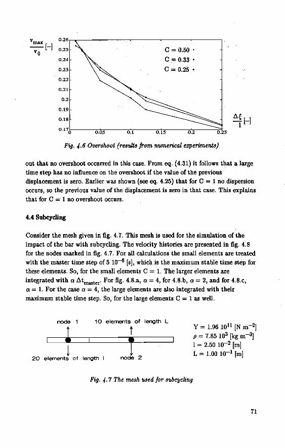
V 0.26 max [-]

0.25 vo 0.24

0.23

0.22

0.21

0.2

0.19

0.18

0.170 0.05 0.1

c = 0.50 +

c = 0.33.

c ~ 0.25 •

0.15

~{ [-] 1

Fig. 4.6 Overshoot (results from numerical ezperiments)

out that no oversboot occurred in this case. From eq. (4.31) it follows that a large time step has no influence on the oversboot if the value of the previous displacement is zero. Earlier was shown (see eq. 4.25) that for C = 1 no dispersion occurs, so the previous value of the displacement is zero in that case. This explains that for C = 1 no oversboot occurs.

4.4 Subcyding

Consider the mesh given in fig. 4.7. This mesh is used for the simulation of the impact of the bar with subcycling. The velocity histories are presented in fig. 4.8 forthenodes marked in fig. 4.7. For all calculations the small elements are treated with themaster time step of 5 10~ [s], which is the maximum stabie time step for these elements. So, for the small elements C = 1. The larger elements are integrated with a ~tmaster· For fig. 4.8.a, a= 4, for 4.8.b, a= 2, and for 4.8.c, a = 1. For the case a = 4, the large elements are also integrated with their maximum stabie time step. So, for the large elements C = 1 as well.

nàde 10 elements of length L

t

T l 20 elements of length node 2

Fig. 4-7 The mesh used for subcycling

Y = 1.96 1011 [N m-2] p = 7.85 103 [kg m-3] 1 = 2.50 10-2 [m] L = 1.00 10-1 [m]

71

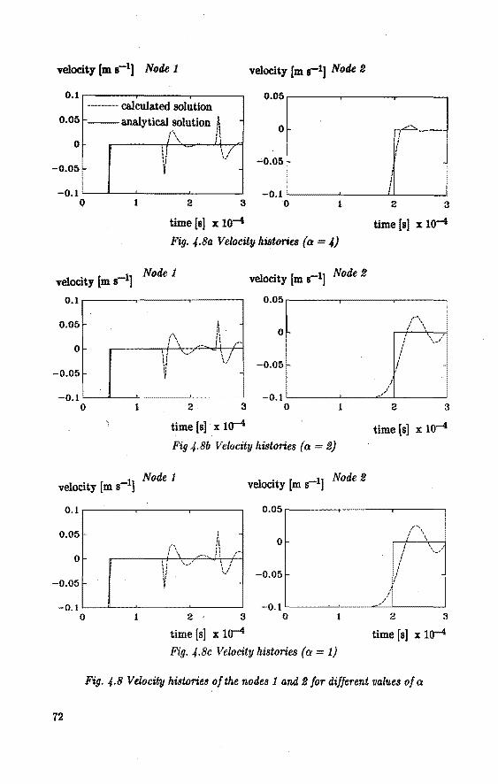
velocity [m a-1] Node 1 velocity [m s-1] Node 14

0.1 .------...----.-------. 0.05 .------.----.....--------. --------- calcula.ted salution

0.05 --a.na.Iytical salution ~ .. {\, ft

0 ol . ' .. . ' .. •.! •I ~ -0.05

'

-0.1 L_____a _ __,_ ___ ....._ __ __J

0 1 2 3

time [s] x Io-4

0

-0.05

-0.1 0 1

Fig. 4.8a Velocity histories (a= 4)

velocity [m a-1] Node 1 velocity [m s-1] Node 2

0.1 0.05

0.05 ft 0 {\ ;\ . \ .: r 0

\I v' .. \-7 •' '• -0.05 ~ -0.05

-0.1 -0.1 0 1 2 3 0 1

time [s] x lo--4 Fig 4.8b Velocity histories (a= 2)

Node 1 velocity [m s-1] velocity [m s-1] Node 2

I

I I I

2 3

time [s] x lo-4

,--, I \ ' '

/ \,.,_/-'

i I '

i _,. 2 3

time [s] x 10-4

0.1 .-------.,.---...,-----, 0.05.--------.-----,----

0.05 l !\

--._ f I /""·

0

0 I \ ... __ /' / -

-0.05 / -0.05

,",/ -0.1 L____ll _ __,_ ___ _._ __ __J -0.1 L--~'---'---."::__L_ __ ___j

0 1 2 3 0 1 2 3

time [s] x 10-4 time [s] x 10-4

Fig. 4.8c Velocity histories (o: = 1)

Fig. 4.8 Velocity histories of the notles 1 and 2 for different values of o:

72

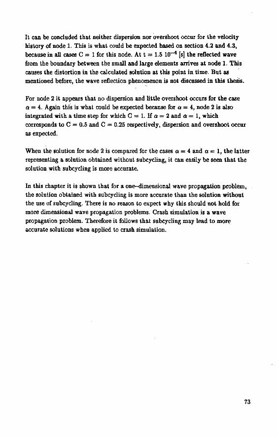
It can he concluded that neither dispersion nor oversboot occur for the velocity histocy of node 1. This is what could be expected based on section 4.2 and 4.3, because in all cases C = 1 for this node. At t = 1.5 1o-4 [s] the reflected wave from the boundary between the small and large elements a.rrives at node 1. This causes the distartion in the calculated solution at this point in time. But as · mentioned before, the wave reDeetion phenomenon is not discussed in this theSis.

. For node 2 it appears that no dispersion and little oversboot occurs for the case a = 4 .. Again this is what could he expected because for a = 4, node 2 is also integrated with a time step for which C = 1. If a = 2 and a = 1, which corresponds to C = 0.5 and C = 0.25 respectively, dispersion and oversboot occur as expected.

When the solution for node 2 is compared for the cases a = 4 and a = 1, the latter repreaenting a solution obtained without subcycling, it can easily beseen that the salution with subcycling is more accurate.

In this chapter it is shown that for a one-dimensional wave propagation problem, the solution obtained with subcycling is more accurate than the solution without the use of subcycling. There is no reason to expect why this should not hold for more dimensional wave propagation problems. Crash simulation is a wave propagation problem. Therefore it follows that subcycling may lead to more accurate solutions when applied to crash simulation.

73

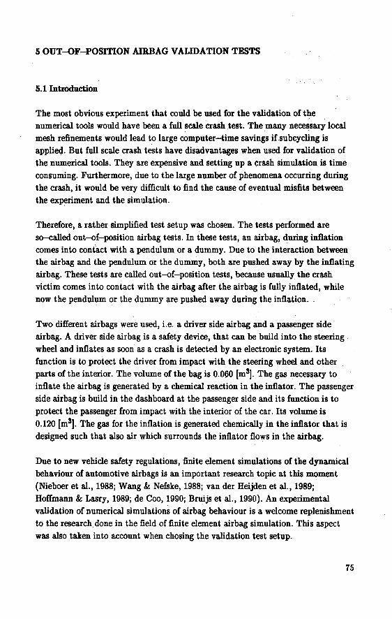
5 OUT-OF-POSITION AIRBAG VALIDATION TESTS

5.1 Introduetion

The most obvious experiment that could be used for the validation of the numerical tools would have been a full seale crash .test. The many necessary local mesh refinements would lead to large computer-time savings ifsubcycling is applied. But full scale crash tests have disadvantages when used for validation of the numerical tools. They are expensive and setting up a crash simwation is time

consuming. Furthermore, due to the large number of phenomena occurring during the crash, it would be very difficult to find the cause of eventual misfits between the experiment and the simulation.

Therefore, a rather simplified test setup was. chosen. The tests performed are so-called out--of-position airbag tests. In these tests, an airbag, during inflation comes into contact with a pendulum or a dummy. Due to the interaction between the airbag and the pendulum or the dummy, bothare pusbed away by the in:Oating airbag. These tests are called out--of-position tests, because usually the crash victim comes into contact with the airbag after the airbag is fully in:Oated, while now the pendulum or the dummy are pusbed away during the in:Oation.

Two different airbags were used, i.e. a driver side airbag and a passenger side · airbag. A driver side airbag is a safety device, that can be build into the steering wheel and in:Oates as soon as a crash is detected by an electronic system. lts function is toproteet the driver from impact with the steering wheel and other partsof the interior. The volume of the bag is 0.060 [m3]. The gas neces~ary to in:Oate the airbag is generated by a chemicá.l reaction in the inflator. The passenger side airbag is build in the dashboard at the passenger side and its function is to proteet the passenger from impact with the interlor of the car. lts volume is 0.120 [m3]. The gas for the in:Oation is generated chemically in the in:Oator that is designed such that also air which surrounds the in:Oator flows in the airbag.

Due to new vehicle safety regulations, fini te element simulations of the dynamica! behaviour of automotive airbags is an important research topic at this moment

(Nieboer et al., 1988; Wang & Nefske, 1988; van der Heijden et al., 1989; Hoffmann & Lasry, 1989; de Coo, 1990; Bruijs et al., 1990). An experimental validation of numerical simulations of airbag behaviour is a welcome replenishment to the research done in the field of fini te element airbag simulation. This aspect was also taken into account when chosing the validation test setup.

75

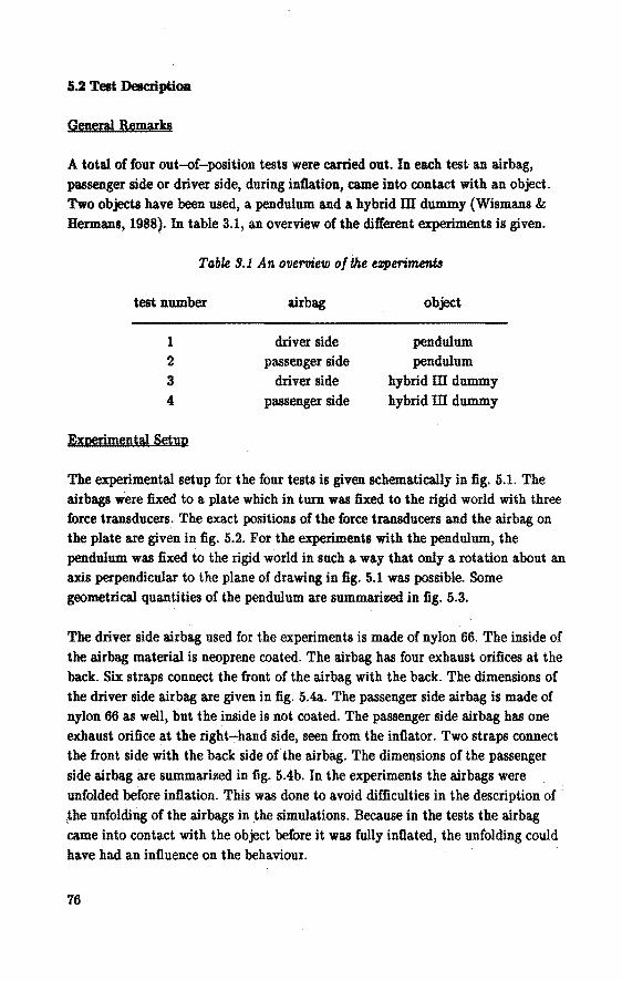
5.2 Test Delcription

General Remarks

A total of four out-of-poBition tests were carried out. In each test an airbag, passenger side or driver side, during inflation, came into contact with an object. Two objecis have been used, a pendulom and a hybrid m dummy (Wismans & Hermans, 1988). In table 3.1, an overview of the different experiment& is given.

Table 3.1 An overuiew ofthe ezperiments

test number

1

2

3 4

Exwimental Setun

airbag

driver side passenger side

driver side passenger side

object

pendulum pendulum

hybrid m dummy hybrid UI dummy

The experimental setup for the four tests is given schematically in fig. 5.1. The airbags were fixed to a plate which in turn was fixed to the rigid world with three force transducers. The exact positions of the force transducers and the airbag on the plate are given in fig. 5.2. For the experiment& with the pendulum, the pendulum was fixed to the rigid world in such a way that only a rotation about an. axis perpendicular to the plane of drawingin fig. 5.1 was possible. Some geometrical quantities of the pendulom are summarized in fig. 5.3.

The driver side airbag used for the experiment& is made of nylon 66. The inside of the airbag material is neoprene coated. The airbag bas four exhaust orifices at the back. Six straps conneet the front of the airbag with the back. The dimensions of the driver side airbag are given in fig. 5.4a. The passenger side airbag is made of nylon 66 as well, but the inside is not coated. The passenger side airbag bas one exhaust orifice at the right-hand si de, seen from the inflator. Two straps conneet the front si de with the back side of the airbag. The dimensions of the passenger side airbag are summarized in fig. 5.4b. In the experiment& the airbags were unfolded before inflation. This was done to avoid difficulties in the description of ~he unfolding of the airbags in the simulations. BtlCause in the tests the airbag came into contact with the object before it was fully inflated, the unfolding could have had an influence on the behaviour.

76

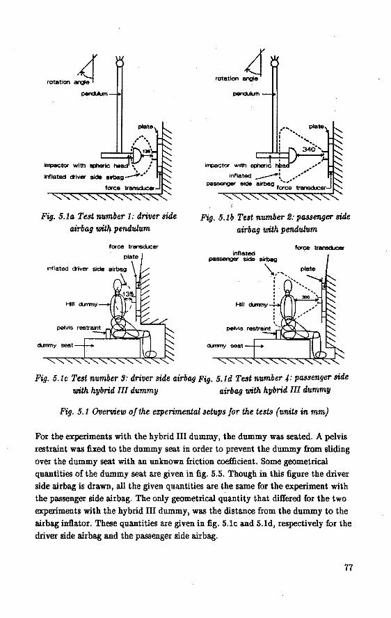
~ter with ~~)~wie head \ /

inflated á'iver aide alrtleg __.. •• •

Fig. 5.1a Test number 1: driver side airbag with pendulum

force transàJc:er

plate

Fig. 5.1b Test number ~: passenger side airbag with pendulum

Fig. 5.1c Test number 9: driver side airbag Fig. 5.1d Test number .;: passenger sitle with hybrid lil dummy airbag with hybrid lil dummy

Fig. 5.1 Overview ofthe experimental setups for the tests (units in mm)

For the experiments with the hybrid III dummy, the dummy was seated. A pelvis restraint was :fixed to the dummy seat in order to prevent the dummy from sliding over the dummy seat with an unknown friction coefficient. Some geometrical quantities of the dummy seat are given in fig. 5.5. Though in this figure the driver side airbag is drawn, all the given quantities are the same for the experiment with the passenger side airbag. The only geometrical quantity that differed for the two experiments with the hybrid III dummy, was the distance from the dummy to the airbag inflator. These quantities are given in fig. 5.1c and 5.1d, respectively for the driver side airbag and the passenger side airbag.

77

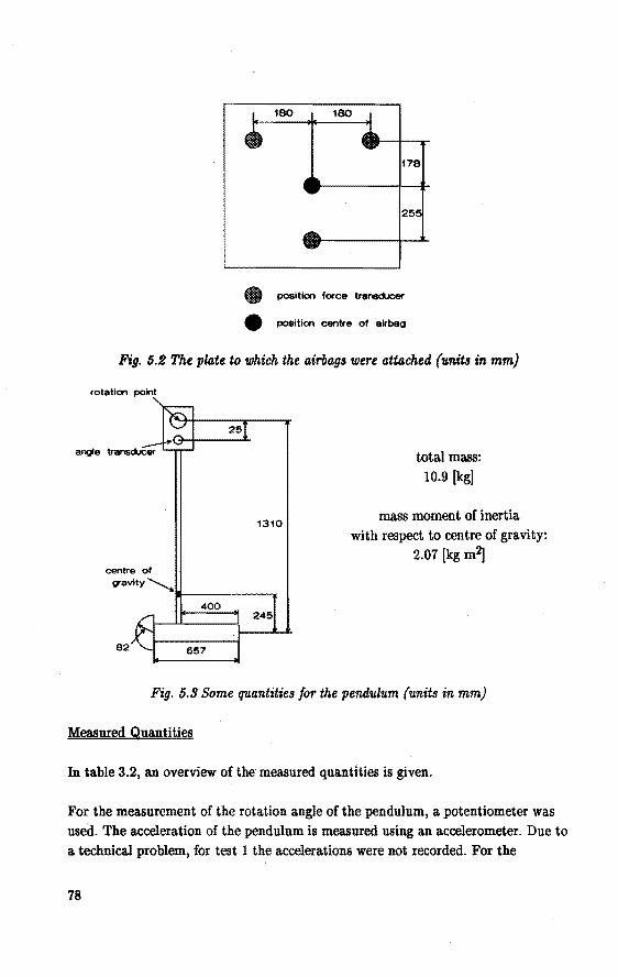
180 180

178

25

4l posltion force transclJcer

• position centre of airbag

Fig. 5.~ The plate to which the airbags were attached (units in mm)

rotatlon point

1310

centre of ~Tavity'-.......

1111--------.: 400

245

82 657

total mass:

10.9 [kg]

mass moment of inertia

with respect to centre of gravity:

2.07 [kg m2]

Fig. 5.9 Some quantities for the pendulum (units in mm)

Measured Ouantities

In table 3.2, an overview of the measured quantities is given.

For the measurement of the rotation angle of the pendulum, a potentiometer was

used. The acceleration of the pendulum is measured using an accelerometer. Due to

a technica! problem, for test 1 the accelerations were not recorded. For the

78

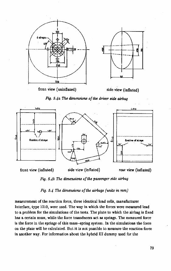
front view (uninflated) side view (inflated)

Fig. 5.,fa The tlimensions of tAe driver sitle airbag

45"0 45"0

~ .........•... !' ··················-

agr a.d].. 1ils:"

\/ 0

fixaüon of atrapa ::; fixalion of llrapl

IJ!:/ .......... ~

.. 1 ····················-··

front view (inflated) side view (in:flated) rea.r view (inflated)

Fig. 5.,fb The tlimensions of the passenger side airbag

Fig. 5.4 The dimensions ofthe airbags (units in mm)

measurement of the reaction force, three identicalload cells, manufacturer Interface, type 1210, were used. The way in which the farces were measured lead to a problem for the simulations of the tests. The plate to which the airbag is fixed has a certain mass, while the force transducers act as springs. The measured force is the force in the springs of this rnass-spring system. In the simulations the force on the plate will be calculated. But it is not possible to measure the reaction force in another way. For information about the hybrid III dummy used for the

79

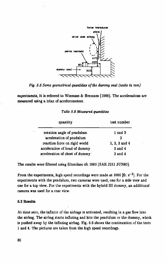
felree tr111'111<iJcer plate

à'iver 8ide ailtleg

,\, I

Fig. 5.5 Some geometrical quantmes ofthe dummy seat (units in mm)

experiment&, it is referred to Wismans & Hermans (1988). The accelerations are measured using a triax of accelerometers.

Table 5.2 Measured quantities

quantity

rotation angle of pendulum acceleration of pendulum

reaction force on rigid world acceleration of head of dummy acceleration of chest of dummy

test number

1 and 2 2

1, 2, 3 and 4 3 and 4 3 and4

The results were filtered using filterclass cfc 1000 (SAE J211 JUNSO).

From the experiments, high speed recordings were made at 1000 [fr. s-1]. For the experiments with the pendulum, two cameras were used, one for a side view and one for a top view. For the experiments with the hybrid III dummy, an additional camera was used for a rear view.

5.3 Results

At time zero, the infl.ator of the airbags is activated, resulting in a gas flow into the airbag. The airbag starts infl.ating and hits the pendulum or the dummy, which is pusbed away by the inflating airbag. Fig. 5.6 shows the continuation of the tests 1 and 4. The pictures are taken from the high speed recordings.

80

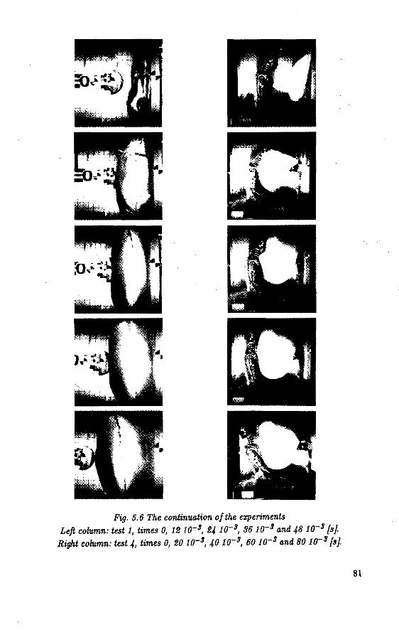
Fig. 5.6 The continuation ofthe experiments Left column: test 1, times 0, 12 10-3, 2.4 10-3, 96 10-3 and 48 10-3 [s].

Right column: test..(, times 0, 20 10-3, 40 10-3, 60 10-3 and 80 10-a [s].

81

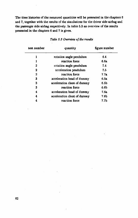
The time histories of the measured quantities will be presented in the chapters 6 and 7, together with the results of the simulations for the driver side airbag and the passenger side airbag respectively. In table 5.3 an overview of the results presented in the chapters 6 and 7 is given.

Table 5.3 Overview ofth.e results

test number quantity tigure number

1 rotation angle pendulum 6.4 1 reaction force 6.6a 2 rotation angle pendulum 7.4 2 acceleration pendulum 7.5 2 reaction force 7.7a 3 acceleration head of dummy 6.5a 3 acceleration chest of dummy 6.5b 3 reaction force 6.6b 4 acceleration head of dummy 7.6a 4 acceleration chest of dummy 7.6b 4 reaction force 7.7b

82

6 SDIULATION OF THE DRIVER SIDE AIRBAG OUT-OF-POSITION

TESTS

6.llntroduction

For the simmations of the experiments with the driver side airbag described in the previous chapter, the driver side airbag was modelled using the triangmar membrane element described in appendix B. For the simmation of the dynamica! behaviour of the airbag, the PISCE8-3DELK code was used. The pendmum and the Hybrid III dummy were modelled using the mmtibody code MADYMO. For the interaction between the airbag and the dummy or the pendmum, the codes were coupled (Buijk, 1989; de Coo, 1990). In MADYMO, the external geometry of the bodies is described with ellipsoids. First the positions and the veloeities of the bodies are updated in MADYMO. The iriformation about the positions and the veloeities was transferred to the PISCES-3DELK code. This code updates the position and the velocity of the nodes and checks them on contact with the ellipsoids as described in section 3.6. The change of momentum of each node is transformed to an external force and moment on the ellipsoid. This procedure is repeated for all ellipsoids. The information about the external forces and moments is transferred to MADYMO and taken into account during the next cycle.

In section 6.2, the models used for the simmation are discussed. The resmts of the simulations, together with the resmts of the tests described in chapter 5, will be presented insection 6.3. Finally, insection 6.4, the resmts will be discussed and conclusions will be drawn.

6.2 Model Setup

Both tests with the driver side airbag were simulated withand without subcycling, yielding a tot al of four simmations { table 6.1)

Table 6.1 An o'l!eruiew ofthe simtdations

simulation number object subcycling

1 pendulum no 2 pendmum yes

3 hybrid lil dummy no 4 hybrid lil dummy yes

83

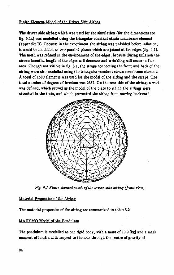
Finite Element Model of the Driver Side Airba&

The driver .side airbag which was used for the simulation (for the dimensions see fig. 5.4a) was modelled using the triangular constant strain membrane element (appendix B). Because in the experiment the airbag was unfolded before inflation, it could be modelled as two parallel planes which are joined at the edges (fig. 6.1). The mesh was refined in the environment of the edges, because during inflation the circumferentiallength of the edges will decrease and wrinkling will occur in this area.. Though not visible in fig. 6.1, the straps connecting the front and back of the airbag were also modelled using the triangular constant strain membrane element. A total of 1680 elements was used for the model of the airbag and the straps. The total number of degrees of freedom was 2532. On the rear side of the airbag, a wall was defined, which served as the model of the plate to which the airbags were attached in the tests, and which prevented the airbag from moving backward.

Fig. 6.1 Finite element mesh ofthe driver side airbag (front view)

Material Properties of the Airbag

The material properties of the airbag are summarized in table 6.2

MADYMO Model of the Pendulum

The pendulum is modelled as one rigid body, with a mass of 10.9 [kg] and a mass moment of inertia with respect to the axis through the centre of gravity of

84

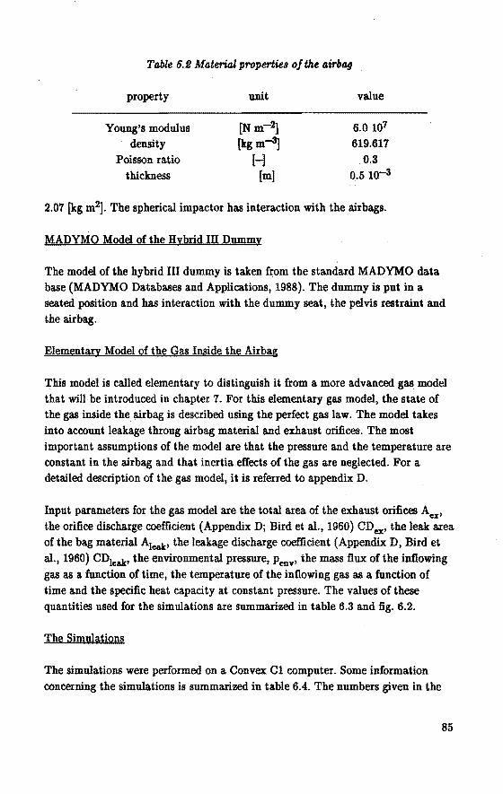
Tabk 6.2 Material properties ofthe airbag

property unit value

Young's modulus [N m-2] 6.0 107

density [kg m-3] 619.617

Poisson ratio H 0.3 thiclmess [m] 0.5 lo-3

2.07 [kg m2]. The spherical impactor bas interaction with the airbags.

MADYMO Model of the Hybrid lil Dummy

The model of the hybrid lil dummy is taken from the standard MADYMO data

base (MADYMO Databases and Applications, 1988). The dummy is put in a

seated position and bas interaction with the dummy seat, the pelvis restraint and

the airbag.

Elementary Model of the GllS Inside the Airbag

This model is called elementary to distinguish it from a more advanced gas model

that will be introduced in chapter 7. For this elementary gas model, the state of

the gas inside the airbag is described using the perfect gas law. The model takes

into account leakage throug airbag material and exhaust orifi.ces. The most

important assumptions of the model are that the pressure and the temperature are

constant in the airbag and that inertia effects of the gas are neglected. For a

detailed description of the gas model, it is referred to appendix D.

Input parameters for the gas model are the total area of the exhaust orifi.ces A ex,

the orifi.ce discharge coefficient (Appendix D; Bird et al., 1960) CD ex, the leak area

of the bag material A1eak, the leakage discharge coefficient (Appendix D, Bird et

al., 1960) CD!eak• the environmental pressure, Penv• the mass flux of the inflowing

gas as a function of time, the temperature of the inflowing gas as a function of

time and the specific heat capacity at constant pressure. The valnes of these

quantities used for the simulations are summarized in table 6.3 and fig. 6.2.

The Simulations

The simulations were performed on a Convex Cl computer. Some information

coneerDing the simulations is summarized in table 6.4. The numbers given in the

85

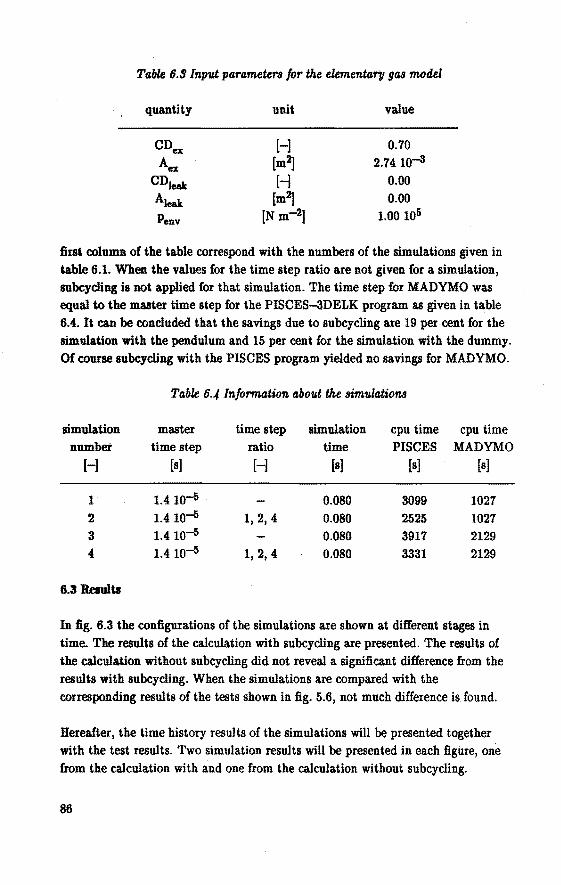
Table 6.9 Input parameters for the elementar'y gas model

quantity

CD ex

A ex

CDleak

Aleak

Penv

unit

H [m2] H

[m2] [N m-2]

value

0.70 2.7410-3

0.00

0.00 1.00 105

first column of the table correspond with the numbers of the simulations given in table 6.1. When the values for the time step ratio are not given for a simulation, subcycling is not applied for that simulation. The time step for MADYMO was equal to the master time step for the PISCES-3DELK program as given in table 6.4. It can be concluded ihai the savings due to subcycling are 19 per cent for the simulation with the pendulum and 15 per cent for the simulation with the dummy. Of course subcycling with the PISCES program yielded no savings for MADYMO.

Table 6.,4 lnformatf.on about the Bimulatf.ons

simulation master time step simulation cpu time cpu time num.bet time step ratio time PISCES MADYMO

H [s] [-] [s] [s] [s]

1 1.41CJÓ . 0.080 3099 1027 2 1.41CJÓ 1, 2, 4 0.080 2525 1027 3 1.410-5 0.080 3917 2129 4 1.4 10-5 1, 2, 4 0.080 3331 2129

6.3 Results

In fig. 6.3 the configura.tions of the simulations are shown at different stages in time. The results of the calculation with subcycling are presented. The results of the calculation without subcycling did not reveal a significant difference from the results with subcycling. When the simula.tions are compared with the conesponding results of the tests shown in fig. 5.6, not much difference is. found.

Hereafter, the time history results of the simula.tions will be presented together with the test results. Two simula.tion results will be presented in each figure, one from the ealcula.tion with and one from the calcula.tion without subcyclîng.

86

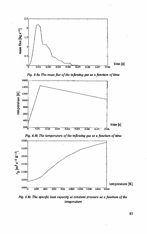
2.5.----.---~--...----:-~-~--.....---~--...,

time [s] 0.05 0.06 0.07 0.08

Fig. 6.fla The ma.ss flux ofthe inflowing gas as a function of time

1~.-----.---~--...---~-~--~-~--...,

time [s]

Fig. 6.tlb The temperature of the inflowing gas a.s a function of time 1300

1250 ~ -I

1200 :::&:::

'1' ... 1150 N

.!. Jl' 1100

temperature [K] 200 400 ~ 800 1000 1200 1400 1~ 1800

Fig. 6.flc The speci.fic heat capacity at constant pressure as a function of the temperature

87

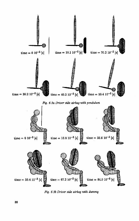
time = 0 to---3 [s] üme- 10.110""" (s]llime- 20.2 104 (s]

time= 30.2 lo---3 [s] üme- 50.4 10""" (s] I Fig. 6.9a Driver side airbag with pend:ulum

time = 0 to-3 [s] time = 33.6 10-3 [s]

Fig. 6.3b Driver side airbag with dummy

88

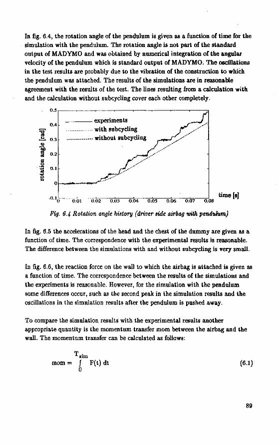
In fig. 6.4, the rota.tion a.ngle of the pendulum is given as a. function of time for the simula.tion with the pendulum. The rota.tion a.ngle is not pa.rt of the sta.ndard output of MADYMO a.nd was obtained by numerical integra.tion of the angnla.r velocity of the pendulum which is ilta.nda.rd output of MADYMO. The oscillations in the test results are proba.bly due to the vibration of the construction to whièh the pendulum was a.tta.ched. The results of the simulations are in reasona.ble agreement with the results of the test. The lines resulting from a calcula.tion with a.nd the calculation without subcycling cover ea.ch other completely.

~ ...=.

t g .... -:; ö ..

0.5

0.4

0.3

0.2

0.1

---experiment& ..................... .,.,.,.,.,.,.,._ with subcycling

·---------~-- without subcycling

·0·1o ---o~o-r-G:o2 o.03 o.04 o.os o.06 o.o7 0.08 time [s]

Fig. 6.4 Rotation o,ngle history (driver side o.irbag 1l1ith pendulum)

In fig. 6.5 the a.ccelerations of the hea.d a.nd the chest of the dummy are given as a function of time. The correspondence with ., the experimental results is reasonable. The difference between the simulations with a.nd without subcycling is vecy small.

In fig. 6.6, the reaction force on the wall to which the airbag is atta.ched is given as a. function of time. The correspondence between the results of the simula.tions a.nd

the experimentsis reasonable. However, for the simula.tion with the pendulum some differences occur, such as the second pea.k in the simulation results a.nd the oscillations in the simulation results after the pendulum is pusbed away.

To oompare the simulation results with the experimental results a.nother appropriate qua.ntity is the momentum transfer mom between the airbag a.nd the wall. The momenturn transfer can be calcula.ted as follows:

Tsim mom= J F(t) dt

0 (6.1)

89

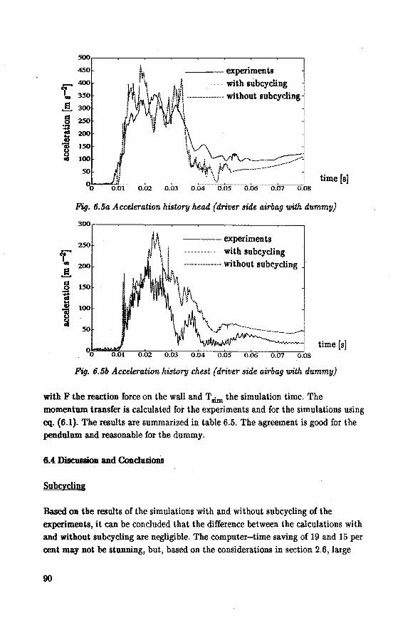
500

450

~ 400 ')' .. 350

..§. 300 R 250 0 .... ':d 200 ~ 8 lSO

$ 100

so

00 time [sJ

0.02 0.03 0.04 0.05 0.06 0.07 0.08

Fig. 6.5a Acceleration history head (driver side airbag with dummv)

300

experiments 250

i' with subcycling ... 200 ·-------------without subcycling

..§. R lSO

v\ 0

\f~\ ~ ~ ~ ~ "' 100 \"' ~ \

so '....P""'-··------time [s]

00 0.06 0.07 0.08

Fig. 6.5b Acceleration history chest (driver side airbag with dummv)

with F the reaction force on the wall a.nd T sim the simula.tion time. The momentnm transfer is calculated for the experiments and for the simulations using

eq. (6.1). The results are summarized in table 6.5. The agreement is good for the pendulnm a.nd reasanabie for the dummy.

6.4 Discussion and Conclusions

Subcycliy

Basedon the results of the simulations with a.nd without subcycling of the experiments, it ca.n be concluded that the difference between the calculations with a.nd without subcycling are negligible. The computer-time sa ving of 19 and 15 per cent may not be stunning, but, basedon the considerations in section 2.6, large

90

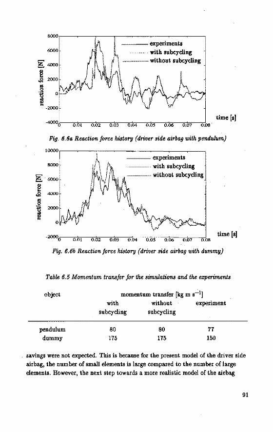
~ ~ .a ~

i

8~,---~--~----.---~----~--~----~--.

6000

-2~

------- experiment& with subcycling

·------------- without subcycling

~%~--o~.0~1--,0~.o~2--'o~.o~3--~o~.M~~o~.o~s--Ao.~~,_-=o.~o7---o~.~ time [sJ

Fig. 6.6a Reaction force h.lstory {driver side airbag with. pendulum)

1~0

8000

6000

4000

2000

-2000i 0

---experiment& """""""""""""""""" with subcycling ·------------- without subcycling

0.01 0.02 0.03 O.M 0.05 0.~ 0.01 0.08 time [s]

Fig. 6. 6b Re action force h.lstory (driver side airbag with. dummy)

Table 6.5 Momenturn transfer for th.e simulations and th.e ezperiments

object momentum transfer [kgm s-1] with without experiment

subcycling subcycling

pendulom dummy

80 175

80 175

77 150

savings were not expected. This is because for the present model of the driver side airbag, the number of small elements is large compared to the number of large elements. However, the next step towards a more realistic model of the airbag

91

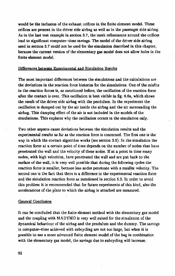
would be the inclusion of the exhaust orifices in the fini te element model. These orifices are present in the driver side airbag as wellas in the passenger side airbag. As in the last test exam.ple in section 3. 7, the mesh refinements around the orifices lead to significant computer-time savings. The model of the driver side airbag used insection 3. 7 could not be used for the simulation described in this chapter, because the current version of the elementary gas model does not allow holes in the

finite element model.

Differences between Expertmental and Simwation Results

The most important differences between the simulations and the calculations are the deviations in the reaction force histories for the simulations. One of the misfits in the reaction forces is, as mentioned before, the oscillation of the reaction force alter the contact is over. This oscillation is best visible in fig. 6.6a, which shows the result of the driver si de airbag with the pendulum. In the experiment the oscillation is dam.ped out by the air inside the airbag and the air surrounding the airbag. This damping effect of the air is not included in the models of the simulations. This explains why the oscillation occurs in the simula.tion only.

Two other aspects cause deviations between the simwation results and the experimental results as far as the reaction force is concerned. The first one is the way in which the contact algorithm worlts (see section 3.6). In the simwation the rea.ction force at a certain point of time depends on the number of nodes that have penetrated the wall and the velocity of these nodes. If at a point in time many nodes, with high veloei ties, have penetrated the wall and are put back to the surface of the wa.ll, it is very well possible that during the following cycles the rea.ction force is smaller, because less nodes penetrate with a smaller velocity. The second one is the fact that there is a difference in the experimental reaction force and the simwation reaction force as mentioned in section 5.2. In order to avoid this problem it is recommended that for future experiments of this kind, also the accelerations of the plate to which the airbag is attached are measured.

General Condusion

It can be concluded that the finite element metbod with the elementary gas model and the coupling with MADYMO is very well suited for the simulation of the

dynamical behaviour of the airbag and the pendulum and the dummy. The savings in computer-time achieved with subcycling are not too large, but when it is possible to use a more ad vaneed finite element model of the bag in combination with the elementary gas model, the sa.vings due to subcycling will increase.

92

7 SIMULATION OF THE PASSENGER SIDE AIRBAG OUT-OF-POSITION

TESTS

7.11ntroducti.on

For the simulations of the tests with the passenger side airbag, the optimization

algorithm (seetion 3.4) determined that subcycling would not result in any oomputer-time savings. For that reasou subcycling is not applied for these

simulations. So the contents of this chapter are actua.lly beyoud the scope of the present research. But, because the simulations with the passenger side airbag are of concern and far from trivial, the results are included in this thesis. n is remarked that, ü the exhaust ori:fice of the passenger si de airbag would have been included in the model, subcycling would lead to substantial computer time savings because of the neeessary mesh refinement around the orifice. But the present

version of the models for the description of state of the gas inside the airbag do not

al.low holes in the finite element mesh. As a preparation to simulations in which the ori:fices can be included in the :finite element model, these simulations are useful. The airbags were again modelled using the triangular constant strain membrane element. The PISCES-3DELK code was used for the simulation of the dynamical beha.viour of the airbag and the MADYMO code for simula.tion of the behaviour of the pendulum and the dummy. The codes were again coupled to account for the interaction between the airbag and the dummy or the pendulum (see section 6.1).

lt will turn out that the elementary gas model which wa.s used for the simulations

with the driver side airbag, does not yield satisfying results for the simulations with the pa.ssenger side airbag. That is why the test with the pa.ssenger side airbag

and the pendulum is also simulated with a more advanced ga.s model to find out

whether this would lead to better results. This simulation should be regarded a.s a first attempt to use this gas model for out-of-position airbag simulation.

The simulation models are discussed in section 7 .2. The results are presented in

seetion 7.3 together with the experimental results. Insection 7.4, the results will be discussed and conclusions will be drawn.

7.2 Model Setup

The test with the pa.ssenger side airbag and the pendulum is simulated with the

elementary gas model and the advanced ga.s model. The test with the pa.ssenger

93

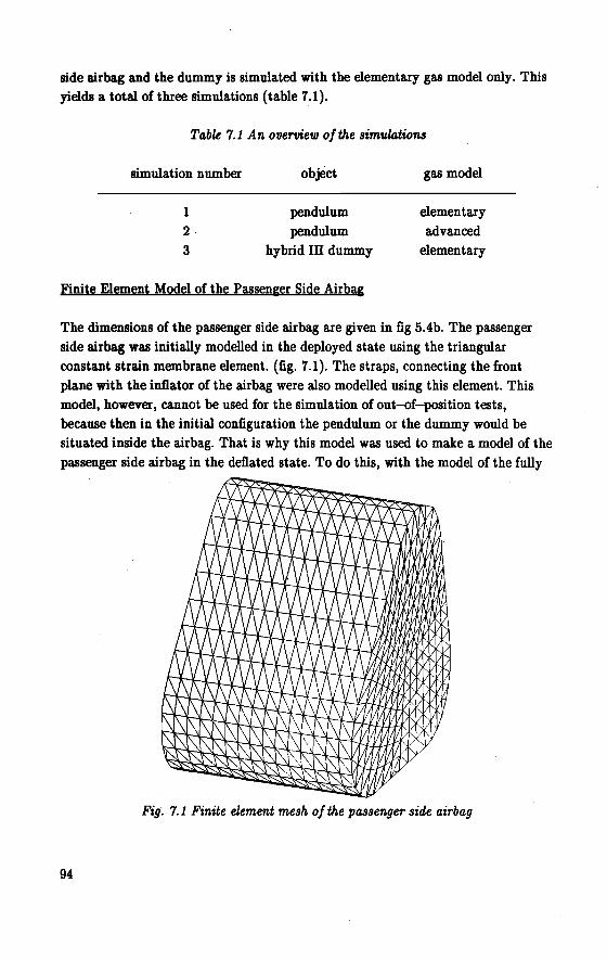
side airbag and the dummy is simulated with the elementary gas model only. This yields a total of three simulations (table 7.1).

Table 7.1 An overoiew ofthe simulations

simulation number object

1 pendulum 2 pendulum 3 hybrid lil dummy

gas model

elementary ad vaneed

elementary

Finite Element Model of the Passenger Si de Airbag

The dimensions of the passenger side airbag are given in fig 5.4b. The passenger side airbag was initially modelled in the deployed state using the triangular constant strain membrane element. (fig. 7.1). The straps, connecting the front plane with the inflator of the airbag were also modelled using this element. This model, however, cannot be used for the simulation of out-of-position tests, because then in the initial configuration the pendulum or the dummy would be situated inside the airbag. That is why this model was used to make a model of the passenger side airbag in the deflated state. To do this, with the model of the fully

Fig. 7.1 Finite element mesh of the passenger side airbag

94

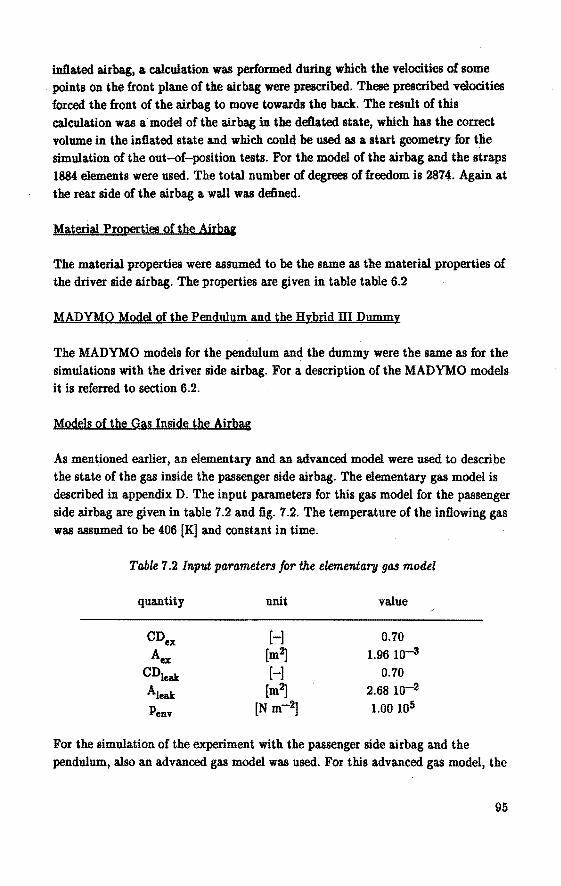
infia~ed airbag, a calculation was performed during which ~he veloeities of some . points on 1ihe front plane of 1ihe airbag were prescri bed. These prescribed veloeities

iorced the fron1i of ~he airbag ~o move towards the back. The result of this

calculation was a model of the airbag in the deflated state, which has the correct

volume in the inflated state and which could he used as a start geometry for the

simulation of ~he out-of-position tests. For the model of the airbag and the straps

1884 elements were used. The total number of degrees of freedom is 2874. Again at

the rear side of the airbag a. wall was defined.

Material Properties of the Airbas

The material properties were assumed to he the sa.me as the material properties of

the driver side airbag. The properties are given in table ta.ble 6.2

MADYMO Model of the Penduturn and the Hybrid III Dummy

The MADYMO models for the pendulum and the dummy were the sa.me as for the

simulations with the driver side airbag. For a description of the MADYMO models

it is referred to section 6.2.

Models of the Gas Inside the Airbag

As mentioned earlier, an elementary and an advanced model were used to describe

the state of the gas inside the passenger side airbag. The elementa.ry gas model is

described in appendix D. The input parameters for this gas model for the passenger

side airbag are given in table 7.2 and fig. 7.2. The temperature of the inflowing gas

was assumed to he 406 [K] and constant in time.

Table 7.2 Input parameters for the elementary gas model

quantity

CD ex

A ex

CDJeak A teak

Penv

unit

H [m~ H [m~

[N m-2]

value

0.70 1.9610-3

0.70 2.68 w-2

1.00 105

For the simulation of the experiment with the passenger side airbag and the

pendulum, also a.n a.dvanced gas model was used. For this advanced gas model, the

95

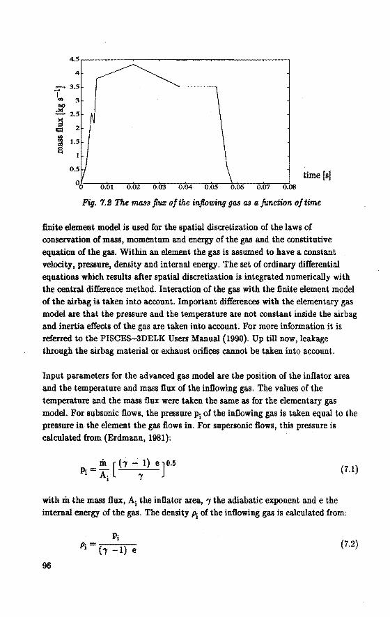
time [s] 0.01 0.02

Fig. 7.! The mass flux ofthe inftowing gas as a fanction of time

fini te element model is used for the spatial discretization of the laws of conservation of mass, momentum and energy of the gas and the constitutive equation of the gas. Within an element the gas is assumed to have a constant velocity, pressure, density and internal energy. 'l'he set of ordinary differential equations which results after spatial discretization is integrated numerically with the central difference method. Interaction of the gas with the finite element model of the airbag is taken into account. Important ditierences with the elementary gas model are that the pressure and the temperature are not constant inside the airbag and inertia effects of the gas are taken into account. For more iniormation it is referred to the PISCES-3DELK Users Manual (1990). Up till now, leakage through the airbag material or exhaust orifices cannot be taken into account.

Input parameters for the ad vaneed gas model are the position of the inflator area and the temperature and mass flux of the in:Oowing gas. The valnes of the temperature and the mass flux were taken the same as for the elementary gas

model. For subsonic flows, the pressure Pi of the in:Oowing gas is taken equal to the pressure in the element the gas flows in. For supersonic flows, this pressure is calculated from (Erdmann, 1981):

= m. [ (1 - 1) e]o.s Pi Ai 1

{7.1)

with m the mass flux, Ai the inflator area, 1 the adiabatic exponent and e the internal energy of the gas. The density Pi of the inflowing gas is calculated from:

(7.2)

96

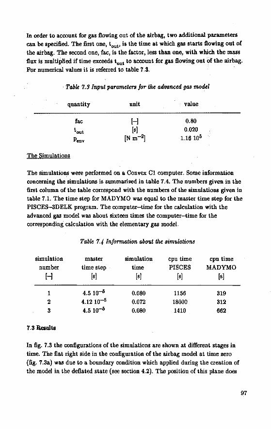
In order to açcount for gas flowing out of the airbag, two additional parameters can be specified. The first one, tout> is the time at which gas starts flowing out of the airbag. The second one, fac, is the factor, less than one, with whiçh the mass flux is multiplied if time exceeds tout to account for gas flowing out of the airbag. For numerical val u es it is referred to ta.ble 7 .3. ,

· Table 1.9 Input parameters for the advanced gas model

quantity

The Simulations

fac

tout

Penv

unit value

0.80 0.020

1.16 105

The simulations were performed on a Convex Cl computer. Some information concerning the simulations is summarized in table 7.4. The numbers given in the first column of the table correspond with the numbers of the simulations given in table 7.1. The time step for MADYMO was equal tothemaster time step for the PISCE8-3DELK program. The computer-time for the calculation with the advanced gas model was about sixteen times the computer-time for the conesponding calculation with the elementary gas model.

Table 1.4 Information about the simulations

simwation master simula.tion cpu time cpu time number time step time PISCES MADYMO

H (s] [s] [s] [s]

1 4.5 10-5 0.080 1156 319 2 4.12 10-5 0.072 18000 312 3 4.5 10-5 0.080 1410 662

7.3Results

In fig. 7.3 the configurations of the simulations are shown at different stages in time. The flat right side in the configuration of the airbag model at time zero (fig. 7.3a) was due toa boundary condition which applied during the creation of the model in the deflated state (see section 4.2). The position of this plane does

97

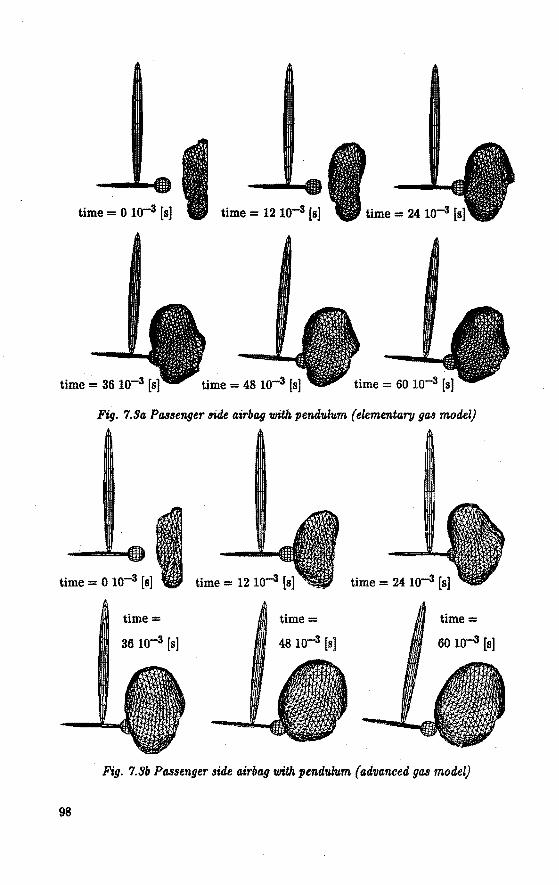
98

üme = 0 10~ [s] time = 12 10~ [s]

Fig. 7.!Ja Passenger side airbag with pend'lllum (elementary gas model}

time=

3610~ [s]

time=

48 10~ [s]

time = 24 10~ [s]

time=

60 10~ [s]

Fig. 1.3b Passenger side airbag with pendulum {advanced gas model}

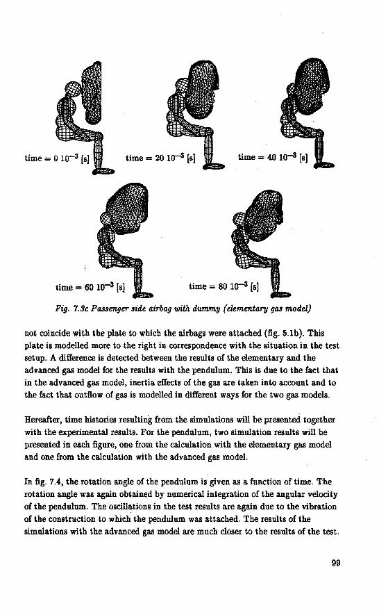
time = 20 to-3 [s] time = 40 10-3 [s)

time= 60 to-3 [s] time = 80 to-3 [s]

Fig. 1.9c Passenger side airbag with dummy (elementary gas model}

not coincide with the plate to which the airbags were attached (fig. 5.lb). This plateis modelled more to the right in correspondencè with the situation in the test setup. A difference is detected between the results of the elementary and the advanced gas model for the results with the pendulum. This is due to the fact that in the advanced gas model, inertia. effects of the gas are taken into account and to the fact that outflow of gas is modelled in different ways for the two gas models.

Herea.fter, time histories resulting from the simula.tions will he presented together with the experimental results. For the pendulum, two simulation results will be presented in each figure, one from the calculation with the elementary gas model and one from the calculation with the advanced gas model.

In fig. 7.4, the rotation angle of the pendulum is given as a function of time. The rotation angle was again obtained by numerical integration of the angular velocity of the pendulum. The oscillations in the test results are again due to the vibration of the construction to which the pendulum was attached. The results of the simulations with the advanced gas model are much closer to the results of the test.

99

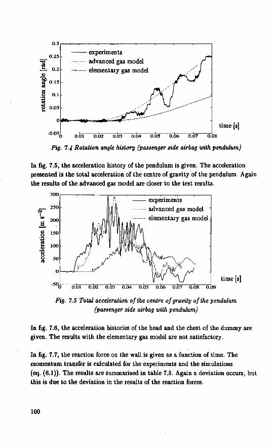
0.3r---~----~--~----~--~----~--~----.

0.25

~ ..!::!. 0.2

..!!:! ~ 0.15 .., g 0.1 ·~ 1\j "§ 0.05

--- experiments · · advanced gas model

·-------- elementary gas model

-0 ·05o 0.01 0.02 0.03 0.04 0.05 0.06 0.07 0.08

time [s]

Fig. 1 . .4 Rotation angle history ( passenger side airbag with pendtdum)

In fig. 7.5, the acceleration history of the pendulum is given. The acceleration presented is the total acceleration of the centre of gravity of the pendulum. Again the results of the ad vaneed gas model are closer to the test results.

r ... .§. = 0 -~ 1\j .... Cl)

~

~

300

250

200

150

100

50

r-, -- experiments

······ advanced gas model ·-------· elementary gas model

-50o 0.01 0.02 0.03 0.04 0.05 0.09

time [s]

Fig. 1.5 Total acceleration ofthe centre of gravity ofthe pend'Ulum ( passenger side airbag with pendulum)

In fig. 7.6, the acceleration histories of the head and the chest of the dummy are given. The results with the elementary gas model are not satisfactory.

In fig. 7.7, the reaction force on the wallis given as a function of time. The

momenturn transfer is calculated for the experiments and the simulations (eq. (6.1)). The results are summarized in table 7.5. Again a deviation occurs, but this is due to the deviation in the results of the reaction forces.

100

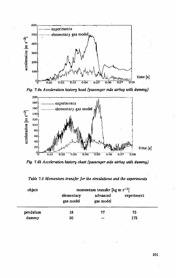
600,---~----~--~--------~----~--~----.

----- experiments 500 --------elementary gas model

A 400

g 300

I 200

100

0 -0

Fig. 7.6a Acceleration history head (passenger side airbag with dummy)

200,---~----~--~----~--~~--~--~----.

180

160

140

120

100

80

60

40

20

---experiments --------- elementary gas model

0.02 0.03

time [sJ 0.05

Fig. 7.6b Acceleration history chest ( passenger side airbag with dummy)

Table 7.5 Momentum transfer for the simulations and the experiments

object

pendulum dummy

momenturn transfer [kgm s-1]

elementary a.dvanced experiment gas model gas model

18 50

77 75

175

101

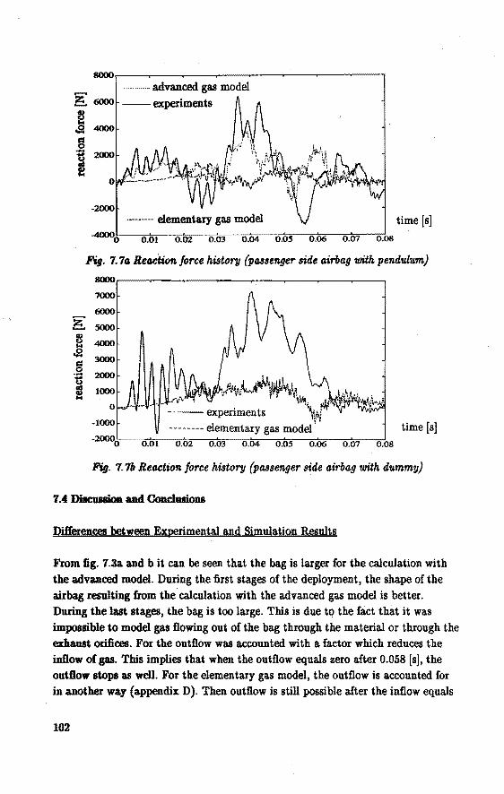
time [s]

0.01 ....... 0.02 0.03 0.04 0.05 0.06 0.07 0.08

Fig. 7. 7a Recction force historg ( passenger side airbag 'With pendu.lum)

8000

7000

6000

~ 5000

8 4000 ... .a 3000 g .... 2000

~

! -1000

-20000

.: I .J.l!\l~JÀ.. . ,..i"J~I.J\w"ill(lf'J'fr'J.lf, ' I \;,i_,

- experiments '\in.t iT

-------- elementary gas model. 0.01 0.02 0.03 0.04 0.05 0.06 0.07 0.08

time [s]

Fig. 7. 76 Reaction force historg ( passenger side airbag 'With dummy)

7.4 Dilleunion and Conclusions

Differences between E:x;perimental and Simulation Results

From fig. 7.3a and bit can beseen that the bag is larger for the calculation with

the advanced model. During the first stages of the deployment, the shape of the

airbag resulting from the calculation with the advanced gas model is better.

During the last stages, the bag is too large. This is due to the fact that it was

impossible to model gas :D.owing out of the bag through the material or through the

exhaust orifices. For the out:D.ow was accounted with a factor which reduces the in:D.ow of gas. This implies that when the outflow equals zero alter 0.058 [s], the out:D.ow stops as well. For the elementary gas model, the outflow is accounted for

in another way (appendix D). Then outflow is still possible alter the inflow equals

102

zero. BaSed on the results of the simulation it can be concluded that too little gas flows out of the airbag. But in the experiment the gas that flows into the airbag fi.rst builds up a pressure inside the airbag and the amount of gas flowing out of the airbag depends again on the pressure inside the airbag. This implies that simply deereasing the amount of gas that flows into the airbag to account for the outflow is not a good model for outflow. Therefore U is recommended that in the advanced gas model outflow of gas can be accounted for dependent on the pressure inside the airbag.

If the rotation angle of the pendulum is considered, U appears that the angular velocity the pendulum reaches is underestimated !or the advanced gas model. The results of the simulation with the advanced gas model are bet ter. The angular velocity the pendulum reaches is 5. 7 [rad s-1] for the simwation with the ad vaneed gas modeland 5.5 (rad s-1] for the experiment.

Regarding the results of the acceleration of the centre of gravity of the pendulum it is again concluded that the results of the simulation with the ad vaneed gas model are better than the results of the simulation with the elementary gas model.

The simulation of the test with the passenger side airbag and the dummy is only performed with the elementary gas model. The simulation results of the acceleration of the head and the chest of the dummy do not oompare with the experimental results.

For the reaction force a large deviation is found between experimental data and the simulation results for the elementary gas model. But the experimental results of the reaction force contain a component that is due to the 'fact that gas is accelerated in the inflator. This component is not included in the reaction force resulting from the simulation with the elementary gas model. The results of the reaction force with the advanced gas model does contain this component. The deviations between these results and the experimental results are due to the same facts as mentioned in section 6.4 for the explanation of the deviation of the reaction force for the driver side airbag. If the momentum transfer is considered, the results of the simulation with the ad vaneed gas model are in agreement with the experimental results.

It can be concluded thàt the elementary gas model is not suited for the simulation of the out-of-position tests with the passenger side airbag. This is due to the fact that in this model the inertia eHects are neglected and the pressure is assumed constant in the airbag. Application of the advanced gas modelleads to good

103

results, though a model that accounts for leakage through airbag material and through exhaust orifices would he more realistie. The way in which the leakage is taken into account for this simulation has disadvantages as mentioned above.

Why the elementary gas model was suited to simulate the out-of-position tests witb the driver side airbag can he explained as follows. In the inflator of the driver side airbag gas is aceelerated. But this gas flows against a face, which is part of the inflator and which causes the gas to flow into the airbag in a direction parallel to the plane to which the airbag is attached. The force exerted on the plate by the . aceelerating gas is compensated by the force exerted on the plate by the face

against which the gas flows. Furthermore, due to the faet that the gas flows into the airbag in a direction parallel to the plate to which the airbag is attached, there is no direct gas flow on the pendulum and the dummy, so the assumption that the pressure is uniform inside the airbag and that the inertia effects can he neglected has less influence for the simulations with the driver side airbag.

General Condusion

The elementary gas model is not suited for the simulation of out-of-poBition tests witb passenger side airbags. The advanced gas model turns out to he suited for simulation of these experiments.

104

8 CONCLUSIONS

8.1 Introduetion

First, in section 8.2 the conclusions concerning the subcycling algorithm are discussed. Afterwards, in section 8.3, the conclusions concerning the simulation of the out-of-position tests with the automotive airbags are considered. Finally, in section 8.4 the overall conclusions are given.

8.2 Snbcycling

Discussion

The subcycling algorithm has been implemented in the PISCES-3DELK program and some test calculations have been performed. Judging from these test calculations it can be concluded that there is hardly any difference between the results of the simulations withor without subcycling. So, subcycling yields no significantlossof accuracy. Furthermore, the test exam.ples showed that for the case in which there are few small elements and many large elements, the savings in computer-time are indeed substantial. If the simulation involves contact and calculations of extemal forces, a decrease of the total computer-time savings will occur. This is due tothefact that only the calculation of the internat forcesis subcycled and the calculation of the external forces and the contacts is not. For more sophisticated elements than the constant strain membrane element, which was used inthetest calcula.tions, the computer-time necessa.ry for the calcula.tion of the internat lorces is much Iarger tha.n the computer-time necessary for the calculation of the external forces and the conta.cts. So if more sophisticated elements are used in the calculations, the decrease of the computer-time saving due to the fa.ct tha.t the calcula.tion of the external forces and the contacts are not subcycled will be much smaller.

If the simulations of the experiments with the driver. side airbag are considered, it can be concluded tha.t there is hardly any difference })et ween the results of a simulation withor a simulation without subcycling. However, COIJ1puter-time savings due to subcycling are not substantial for these simulations, becanse the number of large element& is small and the number of small elements is large.

105

Recommendations for Future Research

In this thèsis only one aspect of subcycling is studied, i.e. the use of different time steps for different elements. But more ways of subcycling can be thought of. For example, when a calculation is made using different programs, like the coupled simulations with MADYMO and PISCEs-3DELK, it is very well possible to use different time steps for both programs. This implies that one of the programs is subcycled compared to the other program. Another way of subcycling involves the uncoupling of different calculations for one and the same element type. H, for example, a shell element is considered, the maximum stabie time step for the calculation of the membrane stresses is usually smaller than the maximum stabie time step for the calculation of the bending stresses. The latter consumes much more computer-time though. Up till now, the time step used for the integration is bounded by the calculation of the membrane stresses. It is possible, however, to use a larger time step for the updates of the bending stresses than for the updates of the membrane stresses. This means that the calculation of the membrane stresses is subcycled compared to the calculation of the bending stresses. Because the former involves much more computer-time than the latter, the savings in computer-time due to this form of subcycling are expected to be large.

8.3 Simulations and Validation Tests

Discussion

When the results of the simulations with the driver side airbag are considered, it can be concluded that they are in good agreement with the results of the experiment&. The overestimation of the momenturn transfer between the driver side airbag and the pendulum is about 3 per cent, while the overestimation of the momenturn transfer between the driver side airbag and the dummy is about 13 per cent. A difference between the simulation and the experiment is the vibration of the airbag in the former afterit is fully inflated. This is visible in the vibration of the reaction force history given in fig. 6.6a. This difference is due to the fact that in reality the vibration is damped out by the air inside the airbag and the air surrounding the airbag. In the simulation the damping effect of the air is not taken into account. Differences in the reaction force history can also be explained by the fact that the resulting reaction force of the simulation is not exactly the same as the measured reaction force, which was discussed before insection 6.4.

For the passenger side airbag the results of the elementary gas model are not satisfactory. This is due tothefact that in the elementary gas model inertia effects

106

of the gas are neglected and the pressure is aasumed uniform in the airbag. Because · the gas flows into the airbag in a direction perpendicular to the plate to which the airbag is attached, the assumptions made for the elementary gas modellead to incorrect simulation results. For that reasou the experiment with the paasenger aide airbag and the pendulum is a.1so simulated with a more advanced gas modèl, in which the inertia effects of the gas are not neglected and in which the pressure inside the airbag can vary. The results of this simulation were better than the results of the simulation with the elementary gas model. The simulation results of the rotation angle of the pendulum and the acceleration of the pendulum are in good agreement with the experimental results. The results of the reaction force deviate from the simulation results. This deviation is probably due to the same fact as the deviations for the reaction force of the simulations with the driver side airbag.

Recommendations for Future Research

As far as the experiment& are concerned, it is recommended that for future experiments of the kind described in chapter 5, also the accelerations of the plate to which the airbag is attached are measured. If these accelerations are known, the reaction force on the plate - which is a aimulation result - can be calculated from the acceleration history of the plate and the force measured by the force transducers.

For simulations with the advanced gas model, it is not possible to model outflow of gas by leakage through the airbag material and through the exhaust orifice. In the present simulation a compensation for this outflow was used by aasuming that less gas flows into the airbag. But in the experiments, gas that flows into the airbag first builds up a pressure inside the airbag. The amount of gas that :flows out of the airbag depends on the pressure inside the airbag. It is recommended that a model is developed to describe outflow of gas dependent on the pressure inside the airbag.

8.4: Concluding Remarb

Subcyclins

In this thesis it is shown that subcycling can indeed lead to substantial computer-time savings, even when it is applied to relatively simple elements like the membrane element. The savings are expected to be larger if subcycling is applied to more complicated elements, especially if different calculations of one element can beuncoupled and subcycled with respecttoeach other. Furihermore

107

it. is shown t.hat. ha.rdly any difference is visible between the results of simulatiollS

with or without subcycling.

It is concluded that subcycling is a metbod that can be used successfully to decrease the computer-times in trallSient finite element analysis, especially when

local mesh refinements are necessary.

Simulation of the Experiment&

The simwation of the tests with the driver side airbag using the elementary gas model yielded satisfying results. For the simulation of the tests with the passenger side airbag, the assumptions made for the elementary gas modelled to incorrect simulation results. The advanced gas model turns out to be suited for the simulation of the tests with the passenger side airbag.

108

REFERENCES

Bathe, K.J. &; Wilson, E.L. (1976). Numerical Methods in Finite Element Analyais. Engtewood Cliffs, New Yersey:' Prentice Hall lnc. ISBN Q-13-62719Q-1.

Bazant, Z.P. (1978). Spurious Reflections of Elastic Waves in Nonuniform Fini te Element Grids. Computer Methods in Applied Mechanica and Engineering, 16, pp. 91-100.

Belytschko, T. &; Mullen, R. (1977). Mesh Partitions of Explicit-lmplicit Time Integration. K.J. Bathe, J.T. Oden&; W. Wunderlich (Eds.), Formulations ofCompv.tational Algorithms in Finite

Element Analyais. MIT Press, Cambridge, Mass.

Belytschko, T. &; Mullen, R. (1978). Stability of Explicit-lmplicit Mesh Partitions in Time Integration. International Joumal for Numerical Methods in Engineering, 12, pp. 1575-1586.

Belytschko, T., Yen, H.-J. &; Mullen, R. (1979).

Mixed Methoeis for Time Integration. Computer Methods in Applied Mechanica and Engineering, 17/18, pp. 259-275

Belytschko, T. (19808).

Partitioned and Adaptive Algorithms for Explicit Time Integration. In: W. Wunderlich, E. Stein &; K.J. Bathe (Eds.), Proceedinga ofthe Ev.rope-U.S. Workshop, Springer Verlag, Berlin, pp. 572-584.

Belytschko, T.B. (1980b).

Explicit Time lntegration of Structural Systems. In: J. Donea (Ed.), Advanced

Strv.ctv.ral Dynamica, Applied Science Publishers, pp. 67-155.

Belytschko, T. &; Hughes, T.J.R. (1983). Computational Methods for Transient Analyais. Mechanics and Mathematica! Methods, A Series of Handbooks. North Holland, Amsterdam: Elsevier Science Publishers B.V. ISBN 0-444-86479-2

109

Belytschko, T., Liu, W.K. & Smolinslà, P. (1983•). Computational Methods for Analysis of Transient Response. Proceed.ings of the 4th ASCE Engineering Mechanit.s Specialty Conference, Purdue University, West

Lafayette, IN, 23-25 May, 1983)

Belytschko, T., Smolinslà, P. & Liu, W.K. (1983b). Stability of Multi-Time Step Partitioned Integrators for First-Order Finite Element Systems. Comp'lder Methods in Applied Mechanics and Engineering, 49,

pp. 281-297.

Belytschko, T., Smolinslà, P. & Liu, W.K. (1984). Multi-stepping ImpHeit-Explicit Procedures in Transient Analysis. In: W.K. Liu,

T. Belytschko & K.C. Park (Eds.), Innovative Methods for Nonlinear Problems, Pineridge Press, Swansea.

Bird, R.B., Stewart, W.E. & Lightfoot, E.N. (1960). Transport Phenomena. London: Wiley. ISBN o-4 71-Q7395-4

Bruijs, W.E.M. (1987). Numerit.al Crash St.mulation of Vehit.le Stroctures, a Literature Survey. Eindhoven University of Technology Research Report. ISBN 9o-6808-o13-X.

Bruijs, W.E.M., Brekelmans, W.A.M., Campen, D.D. van, Coo, P.J.A. de, Heijden, A.M.A. van der, Janssen, J.D. (1988). Computer Time Reduction by Subcycling with an Application to Numerical Crash Analysis. In: C. Marino (Ed.), Supercomputer Applications in Automotive Research and Development. (pp. 347-371). Cray Research Inc., Minneapolis, Minnesota.

Bruijs, W.E.M., Buijk, A.J., Coo, P.J.A. de & Sauren, A.A.B.J. (1990).

Validation of Coupled Calcula.tions with MADYMO and PISCES Airbag. To be published in the Proceedings of the Second International MADYMO Users Meeting, 14 and 15 May 1990, Noordwijk, The Netherlands.

Buijk, A.J. (1989). Input Directives for PISCES Airbag. PISCES Memo ELK3D-Q3. The MacNeal Schwendler Company B.V.

110

Coo, P.J.A. de (1990). MADYMQ-FEM Interfaces. To be publisbed in the Proceedings of the Second

International MADYMO Users Meeting, 14 and 15 May 1990, Noordwijk, The

Netherlands.

Courant, R., Friedriechs, K. & Lewy, B. (1928).

On the Partial Difference Equaüons of Mathematical Physics. Math. Ann, 100,

pp. 82-74.

Erdman, S.F.A.B.P. (1981)

Inleiding supersone aerodynamica (in Dutch). Report D25A, University of

Technology, Delft

Ginsberg, M. & Johnson, J.P. (1989).

Benchmarking the Performance of Physical Impact Simulation Software on Vector

and Parallel Computers. In: J.L. Martin & S.F. Lundstrom (Eds.),

Supercomputing 88: Volume 2- Science and Applications, IEEE Computer Society

Press, Washington, D.C., pp. 18D-190.

Ginsberg, M. & Katnik, R.B. (1989).

Improving Vectorization of a Crashworthiness Code. SAE Technica! Paper Series

891985.

Goldsmith, w. (1960).

Impact, the Theorg and Physical Bekamour of OoUiding Solids. London: Edward

Amold Ltd.

Haug, E., Dagba, A., Clinckemaillie, J, Aberlene, F., Pickett, A., Hoffmann, R. & Ulrich, D. (1988).

Industrial Crash Simulations Using the P AM CRASH Code. Paper presented at the

Conference on Supercomputing in Engineering Structures, IBM Europe Institute

1988. Oberlech, Austria, July 11-15, 1988.

Haug, E. & Ulrich, D. {1989).

The P AM CRASH Code as an Efficient Tool for Crashworthiness Simulaüon and

Design. Paper presented at the 2nd European Cars/Truck Simulation Symposium,

22-24 May, Schliersee, Munich, Germany.

111

Heijden, A.M.A. van der, Buijk, A.J. & Groenenboom, P.B.L. (1989). Numerical Simwation of Airbag Behaviour. Próceedings SUSI Conference, Cambridge, Massachusets, July, 1989.

Hilber, H.M. & Bughes, T.J.R. (1978). Collocation, Dissipa.tion a.nd •overshoot' for Time Integra.tion Schemes in Structural Dyna.mics. Earthquake Engineering and Structural Dynamics, 6, pp. 99-117

Hoeck, H.-G., Poth, A. & Schrepfer, W. (1988). Influence of Modeling Undercarriage and Power Train Components on the Quality of Numerical Crash Simula.tion. In: C. Marino (Ed.), Supercomputer Applications in Automotive Research and Engineering Development, Cray Research Inc., Millnea.polis, Minnesota., pp. 35-45.

Hoffmann, R. & La.sry, D. (1989).

Design for Passive Safety using Numerical Simula.tion Techniques. Symposium on the 50th a.nniversa.ry celebration at the Bioengineering Centre, Wayne State University, Detroit, Mi., November 1989.

Bughes, T.J.R & Liu, W.K. (1978a).

Implicit_.Explicit Finite Elementsin Tra.nsient Analysis: Stability Theory. Joumal of Applied Mechanica, 45, pp. 371-374

Hughes, T.J.R & Liu, W.K. (1978b).

Implicit-Explicit. Finite Element.s in Transient Analysis: Implementation a.nd Numerical tx&mples. Joumal of Applied Mechanica, 45, pp. 375-378

Bughes, T.J.R., Pister, K.J. &; Taylor, R.L. (1979).

Implicit-Explicit Finite Elementsin Nonlinear Tra.nsient Analysis. Computer Methods in Applied Mechanica and Engineering, 17/18, pp. 159-182.

Hughes, T.J.R. (1983).

Analysis of Tra.nsient Algorithms with Partienlar Reference to Stability Behaviour. In: T. Belytschko &; T.J.R. Bughes (Eds.), Computational Methods for Transient Analysis, North Holland, pp. 67-155.

Krieg, R.D. & Key, S.W. (1973}.

Transient Shell Response by Numerical Time Integration. International Joumal of Numerical Methods in Engineering, 7, pp. 273-286.

112

Liu, W.K. &; Bely1schko, T. (1982). Mixed Time Implicit-Explicit Finite Elements f'or Transient Analysis. Computers & Structures, 15, pp. 445-450.

Liu, W.K. & Lin, J.I. (1982). Stability of' Mixed Time lntegration Schemes f'or Transient Thermal Analysis. Numerical Heat Transfer, 5, pp. 211-222.

Liu, W.K., Belytschko, T. & Zhang, Y.F. (1984). Implementation and Accuracy of Mixed-Time Implicit-Explicit Methods for Structural Dynamica. Computers & Strv.ctures, 19, pp. 521-530.

MADYMO Databases and Applications. (1988). Version 4.2. TNO Road-Vehicles Research Institute, Department of Injury Preven ti on.

MADYMO User's Manual 2D. (1988). Version 4.2. TNO Road-Vehicles Research Institute, Department of Injury Prevention.

MADYMO User's Manual 3D. (1988). Version 4.2. TNO Road-Vehicles Research lnstitute, Department of' Injury Prevention.

Newmark N.M. (1959). A Method of Computation for Structural Dynamics. A.S.C.E., Journalof Engineering Mechanica Division, 85, pp. 67-94.

Nieboer, J.J., Wismans, J. & Fra.terman, E. (1988). Status ofthe MADYMO 2D Airbag Model. SAE Technical Paper Series 881729. 32nd Stapp Car Crash Conference, Atlanta

Nilsson, L. {1989). Computational Crash Analysis at the Sa.ab Ca.r Division. Twelfth International Technica! Conference on Experimental Safety Vehicles, May 29- June 1 Göteborg, Sweden, 1989. Proceedings, Vol. 1, pp. 349-388.

113

Park, K.C., Felippa, C.A. & DeRuntz, J.A. (1977). Stabilization of Staggered Solution Procedures for Fluid-8tructure Interaction Analysis.ln: T. Belytschko & T.L. Geers (Eds.), ASME Applietl Mechanics Symposia Series, AMD-Vol. 26. pp. 94-124.

Park, K.C. (1980). Partitioned Transient Analysis Procedures for Coupled-Field Problems: Stability Analysis. Joumal of Applieà Mechanics, 47, pp. 470-476.

Park, K.C. & Felippa C.A. (1980). Partitioned Transient Analysis Procedures for Coupled-Field Problems: Accuracy Analysis. Joumal of Applieà Mechanics, 47, pp. 919-926.

PISCE8-3DELK User's Manual. (1990). The MacNeal-8chwendler Company B.V.

SAE, (1980). Instrumentation for Impact Tests. SAE J211 JUN80, SAE Recommended Practice.

Wang, J.T. & Nefske, D.J. (1988). A New CAL3D Airbag Inflation Model. SAE Teehuical Paper Series 880654. International Congress and Exhibition, Detroit, Michigan.

Wismans, J.S.H.M & Hermans, J.H.A. (1988). MADYMO 3D Simulations of Hybrid UI Dummy Sled Tests. SAE Technical Paper Series 880645. International Congress and Exposition, Detroit, Michigan.

114

APPENDIX A: THE STABILITY OF THE CENTRAL DIFFERENCE

METBOD

In section 2.3 it is stated tbat an integration metbod can be written in tbe fonD.:

(A.1)

Tbe scalar relations for tbe central difference metbod are:

inH/2 = in-1/2 + Llt Xn (A.2)

(A.3)

If tbe central difference metbod is applied to:

(A.4)

tbe equations (A.2), (A.3) and (A.4) can be written in tbe form (A.1) witb:

(A.5)

Tbe eigenvalnes p. of tbe matrix Rare:

1 1 P.t = 1-- J:lt2 w2 +- Llt w (-4 + J:lt2 tJl)l/2

2 2 (A.6)

1 . 1 Ji.2 = 1 -- Llt2 w2-- Llt w ( -4 + J:lt2 tJl)l/2

2 2 (A.7)

If Llt < 2/w, tbe eigenvalnes of R forma conjugate complex pair. Tbe norm oftbe

eigenvalnes is tben:

(A.8)

If Llt = 2/w, tbe eigenvalnes arerealand equal and:

(A.9)

If Llt > 2/w, botb eigenvalnes are real. Tben tbe speetral radius (defined in

115

eq. {2.25)) is:

(A.lO)

wbich islarger than one for .M > 2/w.

Using the stability de:tinitions of section 2.3, it can be concluded that the central difference method is stabie if and only if: J

116

2 .àt <­

w (A.ll)

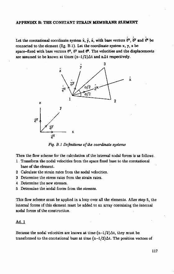
APPENDIX B: TBE CONSTANT STRAIN MEMBRANE ELEMENT

. . . Let the corotationat coordinate system i:, j, i, with base veetors i!X, ~Y and ~ ~e conneeled to the element (fig. B.l). Let the coordinate system x, y, z be space-fixed with base veetors i!X, ~ and ~. The veloeities and the displacements

are assumed to be known at times (n-1/2)~t and n~t respectively.

3

z

x

z y

x

Fig. B.l Definitions ofthe coordinate systems

Then the flow scheme for the catculation of the internat nodat forces is as follows. 1 Transfarm the nodat veloeities from the space fixed base to the corotationat

base of the element. 2 Catculate the strain rates from the nodat velocities. 3 Determine the stress rates from the strain rates. 4 Delermine the new stresses. 5 Determine the nodat forces from the stresses.

This flow scheme must be applied in a loop over all the elements. After step 5, the internat forces of this element must be added to an array containing the internat nodal forces of the construction.

Because the nodat veloeities are known at time (n-l/2)ót, they must be transformed to the corotationat base at time (n-1/2)~t. The position veetors of

117

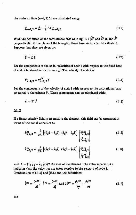
the nodes at time (n-l/2).6t are calculated using:

1 . ~-1/2 = ~- 2 .6t În-1/2 (B.l)

. . -With tàe definition of the corotational base as in fig. B.l ('@X and eY in and ez perpendicular to the plane of the triangle), these base veetorscan be calculated. Suppose that they are given by:

(B.2)

Let the components of the nodal veloeities of node i with respect to the fixed base of node i be stored in the column t. The velocity of node i is:

. ·T v~-112 = ~-1/2 ~ (B.3)

Let the component& of the velocity of node i with respect to the corotational base be stored in the column ;ii. Thesecomponentscan pe calculated with:

(B.4)

If a linear velocity field is assumed in the element, this field can be expressed in terms of the nodal veloeities as:

•yr 1 [<• • · ") (" · • ")] ["2yr l vn-1/2 = 2A YsX- X3Y XaY- Y2X vn-1/2

•2yr vn-1/2

with A= (:i:2 j 3 - :i:3 j-2)/2 the area of the element. The extra superscript r indicates that the veloeities are taken relative to the velocity of node 1.

Combination of (B.5) and {B.6) and the definitions:

118

. avxr . avyr . avxr avyr Êxx = -- êYY = --, and 2fXY = --+ --

OX I oy oy Oi:

(B.5)

(B.6)

(B.7)

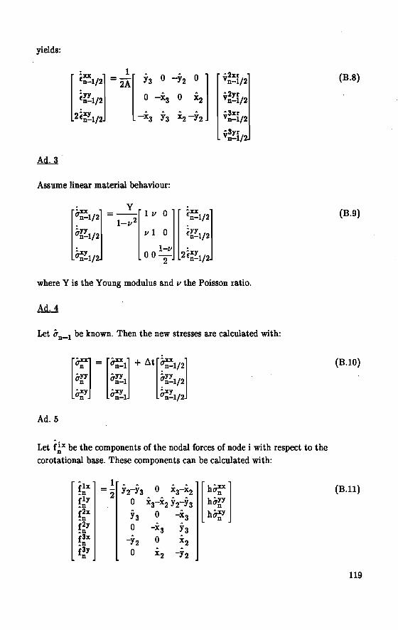
yields:

y3 o -Y.2 o l o -i3 o ~

-xa Ya x2 -y2

·2xr vn-1/2

•2yr vn-1/2

•3xr vn-1/2

•3yr vn-1/

Assume linear material behaviour:

~ y ~1/j =- 1v 0 . 1-v2

Û~1/2 V 1 0

· 1-v ~1/ 002

·xx fn-1/2

f~~1/2

2~~~1/2

where Y is the Young modulus and v the Poisson ratio.

Let ûn_1 be known. Then the new stresses are calculated with:

[~• n = [~1] + ~t[~1/2] q~ q~~1 q~~1/2

~y ~yl ~yl/2 n n- n-

Ad. 5

Let f!x be the componentsof the nodal forcesof node i with respect to the

corotational base. Thesecomponentscan be calculated with:

{1x 1 [h?l .n =2 Y2-Y3 0 X3-X2 hû~Y f1Y 0

... .. ... .. .n xa-x2 Y2-Y3 f2X Ya 0 -x a h~Y .n n f2Y 0 -x a Ya .n f3X .n -y2 0 x2 f3Y n 0

. x2 -y2

(B.8)

(B.9)

(B.10)

(B.U)

119

where h is the thickness of the element. The component of the noda.l forces with respect to the global base for node i are fx, fY and fis. These component& can be calculated from the components with respect to the corotational base with:

(B.12)

Finally it is remarked that the assumption is made that the deformations in the corotational coordinate system must be small. This means that ~. y2, .i:3, y3 and A are constant in the time.

120

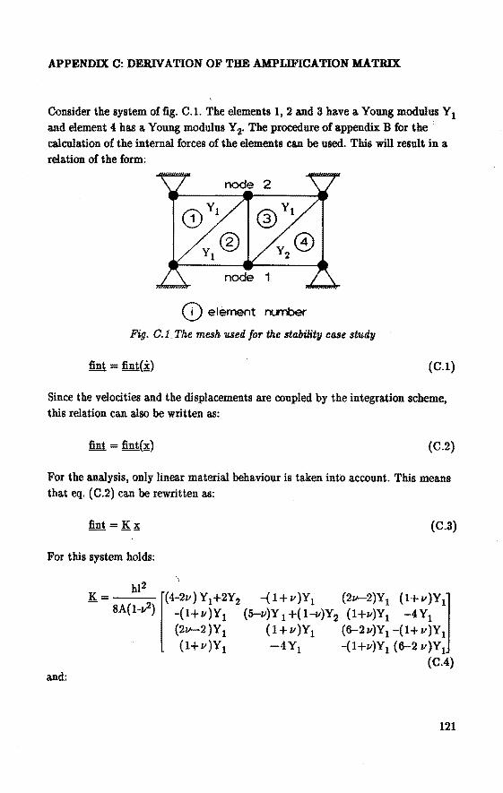
APPENDIX C: DERIV ATION OF TBE AMPLIFICATION MATRIX

Consider the system of fig. C.l. The elements 1, 2 and 3 have a Young modulus Y1 and element 4 has a Young modulus Y 2• The procedure of appendix B for the · calculation of the internal forces of the elements can be used. This will result in a relation of the form:

(D element runber

Fig. 0.1. The mesh 'll.Sed for the stability case study

fint = fint(i;) (C.1)

Since the veloeities and the displacements are coupled by the integration scheme, this relation can also be written as:

(0.2)

For the analysis, only linear material behaviouristaken into account. This means that eq. (0.2) can be rewritten as:

(C.3)

For this system holds:

hl2 l

K = [(4-2v)Y1+2Y2 -(1+v)Y1 (2v-2)Y1 (1+v)Y1] 8A(l-v2) -(l+v)Y1 (5-v)Y 1 +( 1-v)Y2 (1+v)Y1 -4 Y1

(2v-2)Y1 (1+v)Y1 (6-2v)Y1 -(l+v)Y1 . (l+v)Y1 -4Y1 -(1+v)Y1 (6-2v)Y1

(C.4) and:

121

(C.5)

with Y1 the Young modulus ofihe elements 1, 2 and 3 and Y2 the Young modulus

of the element 4. The equations of motion are given by:

(C.6)

with:

M = [ pAh 0 0 0 l 0 pAh 0 0 0 0 pAh 0 0 0 0 pAh

(C.7)

Combination of (C.3), {C.4), (C.5), (C.6), (C.7) and the computations duringa

cycle as given in eqs. (3.3) up to and including (3.14) and (3.16), after elimination

of the veloeities yields:

1 x _ (2 K ) lx lx Xii+l - -cl 11 Xii - Xii-1-

(C.8)

1x _ (2 K ) lx lx Xii+2 - -cl 11 Xii+l - xn -

(C.9)

up to:

(C.lO)

and:

(C.ll)

(C.12)

122

up to:

(C.13)

a.nd:

x2x = (2 _ c K )x2x _ x2:x _ --n+a 2 33 n --n-a

(C.14)

(C.15)

j = 1, 2, ... ,a-1 (C.16)

j = 1, 2, ... ,a-1 (C.17)

with:

(C.l8)

a.nd:

(C.19)

a.nd Kij is the element of K on the ith row a.nd the jth column. These equations ca.n be written in the form:

with:

a.nd:

T 2 T T T T v = [v X v2Y vlx vlY ] ~n ~n •~n •~n •~n

(C.20)

(C.21)

123

2xT _ [ 2x 2x · 2x ] In - Xii+a• Xii+a-l,. .. •Xii-a+l (C.22)

2yT- [ 2y 2y 2y ] Iii - Xii+a• xn+a-l•· .. ,Xii-a+l (C.23)

lxT_[lx lx lXJ In - Xii+a• Xii+a-1,. .. , Xii. (C.24)

lyT _ [ ly ly lY] In - Xii+a• Xii+a-1•···• Xii. (C.25)

and:

A(j,j) = 1 j = 1,2, ... ,6a+2 (C.26)

A(j+l,l) = a

j = 1,2, ... ,a-l (C.27)

A(2a+j+1,2a+l) = a

j = 1,2, ... ,a-1 (C.28)

A(4a+j,j+l) = c1 K13 j = 1,2, ... ,a (C.29)

A(4a+j,2a+l+j) = c1 K14 j = 1,2, ... ,a (C.30)

A{4a+j,4a+l+j) = c1 K11 - 2 j = 1,2, ... ,a (C.31)

A(4a+j,5a+2+j) = c1 K12 j = 1,2, ... ,a (C.32)

A(Sa+j+l,j+l) = c1 K23 j = 1,2, ... ,a (C.33)

A(5a+j+1,2a+l+j) = c1 K24 j = 1,2, ... ,a (C.34)

A(5a+j+1,4a+l+j) = c1 K21 j = 1,2, ... ,a (C.35)

A(5a+j+1,5a+2+j) = c1 K22 - 2 j = 1,2, ... ,a (C.36)

B{l,a) = 2- ~ K33 (C.37)

B{1,2a) = -1 (C.38)

B{1,3a) = -c2 K34 (C.39)

124

B(l,5a) = ~ K31 (C.40)

B(l,6a+1) = ~ K32 (C.41)

B(j+1,a) =! a

j = 1,2, ... ,a-1 (C.42)

B(a+j,a-1+j) ~ 1 j = 1,2, ... ,a (C.43)

· B(2a+1,a) = -c2 K43 (C.«)

B(2a+1,3a) = 2- c2 K44 (C.45)

B(2a+1,4a) = -1 (C.46)

B(2a+1,5a) = -c2 K41 (C.47)

B(2a+1,6a+l) = ~ K42 (C.48)

B(2a+l+j,3a) =! a

j = 1,2, ... ,a-l (C.49)

B(3a+j,3a-1+j) = 1 j = 1,2, ... ,a (C.50)

B(4a+j,4a+l+j) = -1 j = 1,2, ... ,a (C.51)

B(5a+1,5a) = 1 (C.52)

B(5a+l+j,5a+2+j) = -1 j = 1,2, ... ,a (C.53)

B(6a+2,6a+1) = 1 (C.54)

All elements of the matrices A and I! which are not mentioned above are equal to zero.

125

APPENDIX D: TBE ELEMENTARY GAS MODEL

D.l Introduetion

With the elementary gas model the internal pressure inside the automotive airbag can be calculated. For this calculation the following phenomena are taken iuto account: - inflow of gas and heat from the inflator; - outflow of gas and heat by leakage through the airbag material; - outflow of gas and heat through holes in the airbag; - the temperature dependenee of the specific heat capacity of the gas.

The laws, descrihing the state of the gas inside the airbag are the same as those given in Wang & Nefske (1988) and the MADYMO User's Manual2D (1988). However, the present model has the following extensions compared with these models: - during inflation, the preesure is a lunetion of time; - when the airbag is fully deployed, the volume of the bag is not constant and

the end volume need not be specified as an input parameter; - there is no restrietion on the shape of the bag; - straps are easily included; - deformations of the airbag fabric are taken into account; - inertia effects of the airbag fabric are taken into account. The most important simplifications in this model are the assumption that the pressure and the temperature are uniform in the airbag and that inertia effects of the gas are neglected.

During each cycle the volume is calculated from the position veetors of the airbag nodes. Insection D.2, it is described how the pressure can be calculated. Insection D.3, the first law of thermodynamics is used to obtain an equation with which the temperature can be determiued. Section D.4 contains the computations necessary during a cyde.

D.2 Maas Flow

The gas inside the airbag is assumed to he perfect:

mRT p= --::--

V (D.l)

127

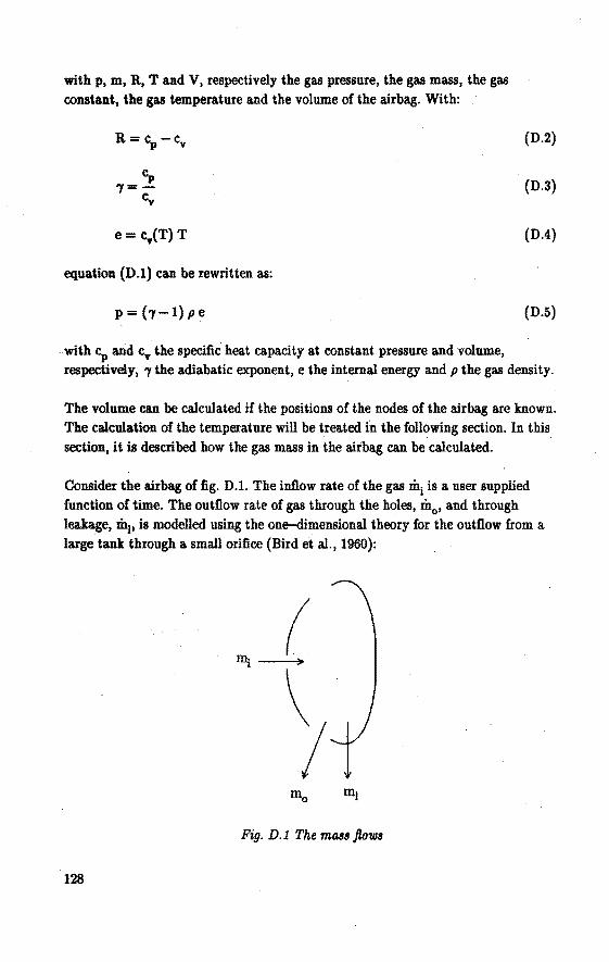
with p, m, R, Tand V, respectively the gas pressure, the gas mass, the gas

constant, the gas temperature and the volume of the airbag. With:

equation (D.l) can be rewritten as:

p=('y-l)pe

(D.2)

(D.3)

(0.4)

(D.5)

with cP and cv the specific heat capacity at constant pressure and volume, respectively, 7 the adiabatic exponent, e the internal energy and p the gas density.

The volume can be calculated if the positions of the nodes of the airbag are known. The calculation of the temperature will be treated in the following section. In this section, it is described how the gas mass in the airbag can be calculated.

Consider the airbag of fig. D.l. The inflow rate of the gas mi is a user supplied function of time. The outflow rate of gas through the holes, m

0, and through

leakage, m1, is modelled using the one-dimensional theory for the outflow from a large tank through a smalt orifice (Bird et al., 1960):

Fig. D.l The mass flows

128

(D.6)

with Aex the area of the exhaust holes, CD ex the orifice discharge coefficient, A1ea.k

the leakage area, CD1ea.k the leakage discharge coefficient and Pexh the pressure at

the exhaust opening. The value of Aex• CDex• A1ea.k and CDleak must be user input.

The pressure at the exhaust opening pexh is approximated by the one-dimensional isentropic expansion of the gas to either the critica! pressure or the environmental pressure according to:

{

Penv Pem =

Pc

ifPenv >Pc (D.7)

ifPenv <Pc

with Pc the critica! pressure defined by (Bird et al., 1960):

7

- [ 2 ]7- 1 Pc- P 7 + 1 (D.8)

The eqs. (D.6), (D. 7) and (D.8) can be used to calculate the mass outflow rates. The mass outflow can be calculated by numerical integration of the outflow rates as described insection D.4. First, insection D.3 the equations for the determination of the temperature will be discussed.

D.3 Calcolation of the Temperature

The first law of thermodynamics states that:

de= dQ-pdV (D.9)

with de the change in intemal energy, dQ the added heat and p dV the work done by the gas. Consider the energy balance of the airbag (fig. D.2):

de = d(m cv(T) T) =

m cv(T) dT + cv(T) T [ rit ] dt + m T dcv(T) (D.lO)

129

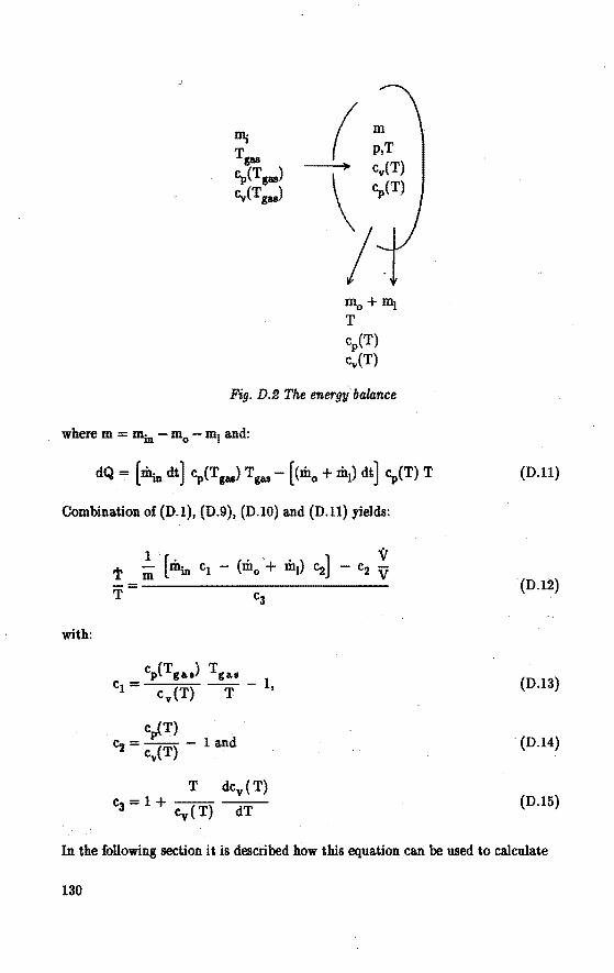
D1j ( m

Tps p,T

c;,(Tgas) <:y(T)

<:y(Tgas) \ c;,(T)

I Fig. D.e The ener!fiÎ balo:nce

(D.ll)

Combination of (D.l), (D.9), (D.lO) and (D.ll) yields:

(D.12)

with:

(D.13)

cp(T) ~ = cv(T) .- 1 and (D.l4)

T dcv(T) c3 = 1 + Cv ( T) dT (D.l5)

In the following section it is described how this equation can be used to calculate

130

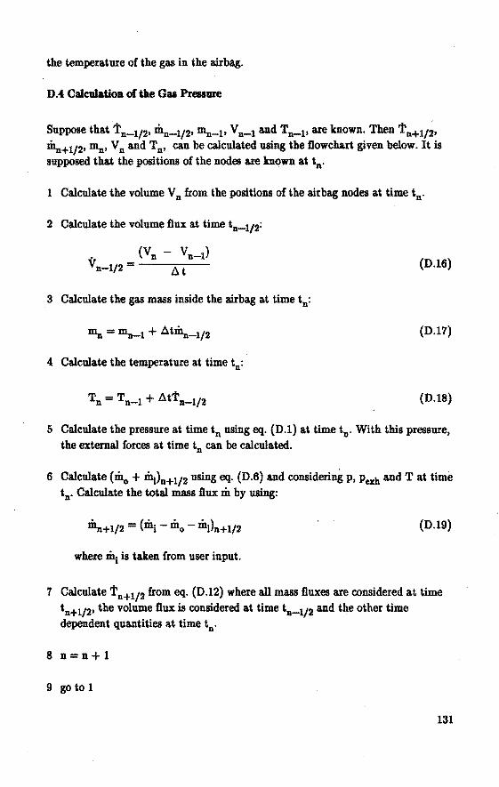
the temperature of the gas in the airbag.

D.4: Cû.culation of the Gas Pressure

Suppose that Tn-l/2, mn-l/2, ~-1 , V n-1 and Tn-l• are ]mown. Then Tn+l/2,

~+l/2, ~·V n and Tn, can be calculated using the :Dowchart given below. It is supposed that the positions of the nodes are ]mown at tn.

1 Calculate the volume V n from the positions of the airbagnodes at time tn.

2 Calculate the volume :Dux at time tn_112:

(D.16)

3 Calcula.te the gas mass inside the airbag at time tn:

(D.17)

4 Calculate the temperature at time tn:

(D.18)

5 Calculate the pressure at time tn using eq. (D.1) at time tn. With this pressure,

the external forces a.t time tn can be calculated.

6 Calcula.te (m0 + m1)n+l/2 using eq. (D.6) and consideriug p, Pexh and T at time tn. Calcula.te the total mass :Dux m by using:

(D.19)

where ~ is taken from user input.

7 Calculate Tn+l/2 from eq. (D.12) where all mass fiuxes are considered at time tn+l/2, the volume fiux is considered at time tn_112 and the other time dependent quantities at time tn.

8 n=n+l

9 gotol

131

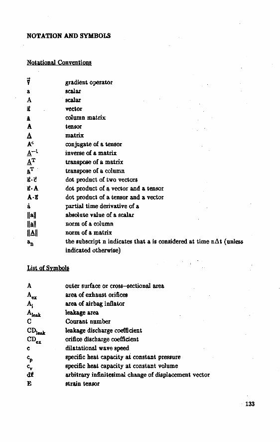
NOTATION AND SYJmOLS

Notational Conventions

V gradient operator a scalar A scalar it veetor il column matrix A tensor A matrix Ac conjugate of a tensor A-l inverse of a matrix AT transpose of a matrix aT transpose of a column it • ~ dot product of two veetors it • A dot product of a vector and a tensor A· it dot product of a tensor and a vector a partial time derivative of a llall absolute value of a scalar 11&11 norm of a column IIAII norm of a matrix 'n the subscript n indicates that a is considered at time n.L\ t ( unless

indicated otherwise)

List of Symbols

A

A ex

~ Aleak c CDlealt CD ex

c CP cv dX E

outer surface or cross-sectionat area area of exhaust orifices area of airbag inflator leakage area Courant number leakage discharge coefticient orifice discharge coefficient dilatational wave speed specific heat capacity at constant pressure specific heat capacity at constant volume arbitrary infinitesimal change of displacement veetor strain tensor

133

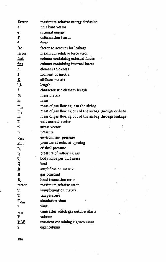
Eerror ~

e F f fac !error

m.n fini h J K l,L l M m

Penv

pexh

Pc

Pi q Q

R R Re rerror

1: T

Tllim t

tout V

YS!l y

134

maximum relaüve energy deviaüon unit base vector internat energy delormation tensor force factor to account for leakage maximum relaüve force error column containing external forces column containing internal forces element thickness moment of inertia stiffness matrix length charaderistic element length mass matrix mass mass of gas flowing into the airbag mass of gas flowing out of the airbag through orifices mass of gas flowing out of the airbag through leakage unit normal vector stress vector pressure environment pressure pressure at exhaust opening critical pressure pressure of inflowing gas body force per unit mass heat amplification matrix gas constant local truncation error maximum relative error transformation matrix temperature simwation time time time after wliich gas outflow starts volume matrices containing eigencolumns eigencolumn

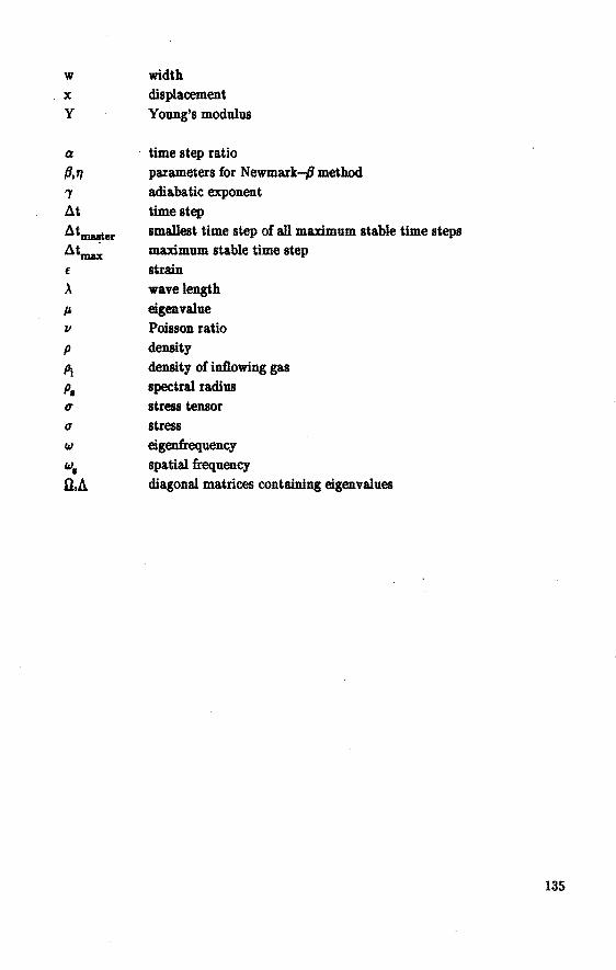
w

x y

a

p," 7 At

Atmaaier Atma.x f

À

p. ll

width displacement Young's modulus

time step ratio parameters for Newmark-{1 method adiabatic exponent time step smallest time step of all maximum stabie time steps maximum stabie time step strain wavelength eigenvalue Poisson ratio densiiy density of inflowing gas speetral radius stress tensor stress eigenfrequency spatial frequency diagonal matrices containing eigenvalnes

135

STELLINGEN

behorende bij het proefschrift

SUBCYCLING IN TRANSJENT FINITE ELEMENT ANALYSIS

1 In de dynamika heeft een expliciete integratiemethode veel voordelen ten opzichte van impliciete methoden bij gebruik van de eindige elementenmethode. Het is bijvoorbeeld veel eenvoudiger niet-lineaire randvoorwaarden in rekening te brengen.

Belytschko, T. & Bughes T.J.R. (1983).Computational Methods for Transient Analysis. Mechanics and Mathematica! Methods, A Series of Handbooks. North Holland, Amsterdam: Elsevier Science Publishers B.V.

Dit proefschrift, hoofdstuk 3.

2 Toepassing van subcycling levert winst. in rekentijd op in het kontakt algoritme.

Dit proefschrift, hoofdstuk 3.

3 Ook indien men een berekening met subcycling uitvoert op een parallelle computer, worden door subcycling aanzienlijke winsten in rekentijd behaald.

Smolinski, P. (1989). Parallel Multi-Time Step In:tegration on a Transputer System. Computers & Stroctures, Vol. 33, No. 6, pp. 1529-1535.

4 Indien de massa van een schaalelement foutief over de knooppunten verdeeld wordt en de uitwendige druk op dezelfde foutieve wijze over de knooppunten verdeeld wordt, zal voor vele problemen geen extra fout worden gei ntroduceerd.

Bughes T.J.R. (1988). The Finite Element Method. Linear Static and Dynamic Finite Element Analysis. Prentice Hall International Editions, London.

5 In de literatuur is het onderzoe1c naar de nauwkeurigheid van de gemengde integratiemethoden achtergebleven bij het onderzoek naar de stabiliteit van deze gemengde integratiemethoden.

Dit proefschrift, hoofdstuk 2.

6 Een goede regulering van overheidswege kan voorkomen dat duurdere passieve veiligheidsmiddelen slechts dienen ter bescherming van een beperkt deel van de bevolking.

Wismans, J.S.H.M. (1990). Over mechà.nica, letsels en preventie. Intreerede Technische Universiteit Eindhoven.

7 Als er tijdens het promotieonderzoek nauw samengewerkt wordt met derden, werkt dit stimulerend op de onderzoeker. Vooral omdat de kans kleiner is dat de resultaten van het onderzoek ongebruikt blijven.

8 Gezien de gang van zake bij promotieonderzoeken door assistenten in opleiding en het doel van stellingen, dienen stellingen te worden afgeschaft.

9 De aanhef' On in titels van proefschriften is volstrekt overbodig.

10 Een dimensiekontrole is reeds voldoende om het gezegde tijd is geltl te ontkrachten.

Eindhoven, September 1990 Wim Bruijs