Style momentum within the S&P-500 index - DePaul University

www.elsevier.com/locate/econbase

Journal of Empirical Finance 11 (2004) 483–507

Style momentum within the S&P-500 index

Hsiu-Lang Chena,*, Werner De Bondtb

aDepartment of Finance, College of Business Administration, University of Illinois-Chicago, USAbDriehaus Center for Behavioral Finance, DePaul University, Chicago, USA

Available online

Abstract

Investors may be able to benefit from equity style management. We find that three company

characteristics—market value of equity, book-to-market ratio, and dividend yield-capture style-

related trends in equity returns. We study all firms in the Standard and Poor’s-500 index since 1976.

Strategies that buy stocks with characteristics that are currently in favor (past winners) and that sell

stocks with characteristics that are out-of-favor (past losers) perform well for periods up to 1 year and

possibly longer. Style momentum in equity returns is an empirical phenomenon that is distinct from

price and industry momentum.

D 2004 Elsevier B.V. All rights reserved.

Keywords: Style momentum; S&P-500 index; Equity

Investment style is the single most important component of success in active equity

portfolio management. The institutional investment community knows and appreciates

this.1 For example, much of the exceptional performance of the Fidelity Magellan Fund

during the 1980s, under Peter Lynch, was achieved by judicious shifts in style, not by

astute stock picking.2

Many equity managers identify themselves as following a particular style. Consider,

e.g., the proliferation of style indexes and the Morningstar style box. Assets in a style

0927-5398/$ - see front matter D 2004 Elsevier B.V. All rights reserved.

doi:10.1016/j.jempfin.2004.04.005

* Corresponding author. Tel.: +1-312-355-1024; fax: +1-312-413-7948.

E-mail address: [email protected] (H.-L. Chen).1 Arnott et al. (1989) state the matter as follows: ‘‘[S]tyle. . .shapes the pattern of returns more significantly

than virtually any other element in the investment process. We cannot know whether this will be a year that

rewards growth or value investors. But, in a year that rewards value managers, almost all growth managers will

suffer. Conversely, in a year that rewards growth investors, those who favor value will generally suffer.’’ For a

book-length discussion of style investing, see Bernstein (1995).2 See Sharpe (1992). Sharpe relies on a linear model to characterize investment style. This approach reflects

the fact that mutual fund returns are highly correlated with broad asset class returns. Sharpe’s model is widely

used but requires a time-series of historic fund returns. In this paper, we describe investment styles in terms of

stock characteristics.

H.-L. Chen, W. De Bondt / Journal of Empirical Finance 11 (2004) 483–507484

category share common characteristics. Our paper is motivated by the widespread use of

the value/growth and small-cap/large-cap labels. In a study of the mutual fund industry,

Chan et al. (2002) confirm that value/growth (measured by the ratio of book value to

market value of equity) and size (measured by equity capitalization) are, indeed, useful

descriptors of style. This conclusion would hold true for other branches of the money

management industry, we believe.

Style investing is a form of product differentiation. It positions the portfolio to be ‘‘out-

of-sync’’ with the broad market. Investors keep an eye on style purity (Does the trading

strategy match the announced objective?) and style drift, its converse.3 The emphasis on

style allows the industry to organize the investment process better. For instance, style

benchmarks assist in performance evaluation and risk control.

Styles perform differently over time. What was effective a year ago may be

counterproductive today. In 1998 and 1999, growth stocks did spectacularly well but

value stocks performed poorly despite good earnings news. During the first part of 2002,

small capitalization firms kept the Standard and Poor’s-500 index from falling as steeply

as the Nasdaq Composite (Talley, 2002). No single style or mix of styles is optimal for all

periods and circumstances. This is a major worry for anyone in equity management.

However, if one could identify and time a style cycle, it may be possible to earn superior

returns. Birch (1995) explains how, in principle, a plan sponsor can use style cycle

information to perfect tactical asset allocation. Arnott et al. (1989), Fisher et al. (1995),

Kao and Shumaker (1999), Levis and Liodakis (1999), and Lucas et al. (2002) use

historical data to show the potential benefits of style rotation and to examine the cyclical

variation in the risks and returns of style portfolios. These studies are interesting but by

and large they do not pin down the pervasive economic forces, if any, that drive style

dominance or the specific trading strategies suggested by style cycles.4

It is common practice among amateur and expert investors to chase investment styles

that have performed well over the recent past. Since money managers compete for fund

flows, they face powerful incentives to accommodate their clients’ wishes and to adjust

their investment strategies, irrespective of their own beliefs about future risk and return.

Style momentum strategies are a form of style rotation that can serve this purpose. One

buys stocks with characteristics that are currently in favor and one sells stocks with

characteristics that are out-of-favor.

If nothing else, the pressure from clients may sway managers to adjust their fund

marketing. Sirri and Tufano (1998) and Jain and Wu (2000) find that mutual funds that

3 During the 1990s, perhaps as many as 40% of all equity mutual funds were mislabeled in the sense that the

return dynamics were different from the style that was listed in the prospectus (DiBartolomeo and Witkowski,

1997). The business press takes notice of style drift; see, for instance, Tam (2000).4 Arnott et al. (1989) describe changing macro-economic conditions with an index of leading indicators,

producer prices, and the money supply. Kao and Shumaker (1999) focus on consumer prices, the risk and term

structure of interest rates, growth in GDP, and the earnings-to-price ratio for the S&P-500. Levis and Liodakis

(1999) find that inflation is a predictor of the size spread and the value spread. Lucas et al. (2002) use the spread

between long- and short-term interest rates and the leading indicators. With the possible exception of Asness et al.

(2000), none of the studies has much success in forecasting style returns. Asness et al. forecast the future returns

of value and growth strategies with (i) a (mostly backward looking) spread in value indicators, and (ii) the spread

in analyst long-term forecasts of earnings growth.

H.-L. Chen, W. De Bondt / Journal of Empirical Finance 11 (2004) 483–507 485

advertise their superior past performance attract more money. Cooper et al. (2003) show

that mutual funds go so far as to change their names to take advantage of current hot

investment styles. The name change, it appears, stops negative fund flows.5 From an

investor dollar-and-cents perspective, however, the accent on past returns may be

misplaced. Later results typically fall short of relevant benchmarks. The evidence for

economically meaningful short-term persistence in mutual fund performance is scant or

non-existent (Carhart, 1997; Chen et al., 2000).6

A different and more basic rationale for style momentum investing is that the popularity

of style investing itself may influence the structure and dynamics of asset returns. (That,

with limited arbitrage, security prices move in response to changes in investor sentiment is

a line of thought commonly pursued by researchers in behavioral finance.) Barberis and

Shleifer (2003) believe that many investors trade baskets of stocks and move funds

between styles depending on their performance—always chasing past winner styles and

dumping losers. In theory, several consequences follow. One of them is that past style

returns help to explain the cross-section of expected returns for individual stocks. At the

style level, we may find intermediate-term momentum and long-term reversals in prices.7

This study addresses the central empirical question whether equity style cycles actually

exist. In particular, if a style is currently in-favor or out-of-favor, does that fact helps us to

predict future stock returns for individual securities? The issue is closely related to another

matter of interest—whether a small set of basic risk factors can capture the structure and

dynamics of asset returns. Fama and French (1992, 1996) suggest that, with the possible

exception of the momentum strategy examined by Jegadeesh and Titman (1993), cross-

sectional variation in expected equity returns is captured by three pervasive factors with

associated risk premia. The factors are the market portfolio and the mimicking portfolios

for size (SMB) and book-to-market (HML). Some studies doubt whether factor models can

explain the cross-section of expected returns (see, e.g., Roll, 1995). In particular, Daniel et

al. (1997) suggest that firm characteristics—rather than securities’ factor loadings on the

market return, SMB, and HML—determine expected returns.8 Haugen and Baker (1996)

5 ‘‘Window dressing’’ and style drift are not the only forces at work, however. Financial professionals also

face career risk if the performance of their portfolios falls greatly below relevant benchmarks. Chan et al. (2002)

find that few mutual funds take extreme positions relative to the S&P-500 index. Those who do favor growth

stocks and past winners.6 Our appraisal of the data is mildly contradicted by Davis (2001). This author groups mutual funds by equity

style. He relies on past returns and the Fama–French 3-factor model to infer style. Few funds have much of a

value tilt. No group of funds earns subsequent positive abnormal returns relative to the 3-factor model. Still, Davis

finds that there is some short-run performance persistence for the best growth funds and the worst small-cap

funds. The main implication of this and other research remains that one is unlikely to earn abnormal profits by

looking for ‘‘hot hands’’ in mutual funds.7 Other predictions include the following: (i) past fund flows predict future returns; (ii) the good past

performance of one style can damage the prospects of other styles; (iii) stocks with similar style characteristics

comove more than is justified by economic fundamentals; and (iv) stocks that belong to different styles comove

too little. Teo and Woo (2001) offer some evidence of style-related return reversals.8 Company characteristics such as size, price–earnings ratio, etc. are certainly associated with differences in

average returns. However, the question is whether stock characteristics do better than factor risk loadings in

explaining the cross-section of equity returns. Davis et al. (2000) conclude that the evidence of Daniel and Titman

(1997) is special to their sample period.


predict expected returns based on a forecasting model that is updated monthly and that

relies on more than 50 security characteristics related to risk, liquidity, price level, growth

potential and price history. The out-of-sample forecasts are surprisingly accurate over short

horizons. Haugen and Baker question whether the differences in realized returns are risk

related since none of the standard risk factors (that capture the sensitivity to macroeco-

nomic variables) carry much weight.

In this paper, we use an approach that, at yearly intervals over the period between 1976

and 2000, partitions S&P-500 stocks into groups along three firm characteristics: Dividend

yield, market value of equity, and book-to-market ratio. The partition forms the basis for a

style momentum strategy. We rank 10 style portfolios by their returns over the past 3 to 12

months. Securities with in-favor characteristics, we find, later outperform securities with

out-of-favor characteristics. The return differential is significant—in the order of 20 to 60

basis points per month. The drift lasts up to 12 months.

Since we investigate well-established large American firms that are part of the

S&P-500 index, survivorship bias is unlikely to be the culprit. Neither are we culpable

of look-ahead bias. All the investment strategies described in this article are fully

implementable. It is true that style rotation suffers from high turnover and that trading

costs may eat up its incremental returns. We believe nonetheless that the results

remain of practical value, for instance, in the timing of trades, in the allocation of new

funds between equity styles, or in the design of an enhanced index strategy. While we

cannot dismiss the possibility that style momentum is a chance result—due to

(collective) data mining and therefore unlikely to be replicated out of sample—we

are confident that in our sample style momentum is a phenomenon that is distinct

from price momentum and industry momentum. In other words, the findings are not

an artifact. They do not restate in a new way what was found earlier by De Bondt

and Thaler (1985, 1987), Jegadeesh and Titman (1993), Moskowitz and Grinblatt

(1999), and others.

The results present a challenge to behavioral as well as to rational theories. It is not

obvious in which way they follow from models based on rational agents and frictionless

markets. Taken at face value, the findings appear inconsistent with underreaction to firm-

specific news as well, e.g., Bernard’s (1993) research on earnings momentum and the post-

earnings announcement drift.

The study is organized as follows. Section 1 describes the sample and methods. Section

2 evaluates style momentum strategies. Section 3 asks whether the strategies can be

distinguished from price and industry momentum and performs various robustness tests.

Section 4 briefly examines the risk of investment strategies based on style momentum.

Section 5 concludes.

1. Sample and methods

We study the last quarter of the 20th century, i.e., the period between January 1976

and December 2000. As our universe of stocks, we choose all companies that were

part of the Standard and Poor’s-500 index. Monthly return data are collected from the

Center for Research in Security Prices (CRSP) at the University of Chicago.


Corresponding accounting data are gathered from the annual files of Compustat. We

only consider ordinary common equity issues. For instance, real estate investment

trusts are left out.

On December 31 of each year, we segment the sample into 10 style portfolios (P1,

P2, . . ., P10) each comprising securities with similar characteristics. The partitioning

variables are annual dividend yield (DY), market value of equity (ME), and book-to-

market ratio (BM).9 Stocks that did not pay dividends during the year are placed in

portfolio P10. All other stocks are ranked independently by their year-end market

capitalization and book-to-market ratio.10 They are allocated to three equal-sized ME

groups and three equal-sized BM groups. Firms with negative book value or with a

share price below US$1 at the time of portfolio formation are excluded.11 What portfolio

at the intersection of ME and BM a firm belongs to and whether it is a member of the

S&P-500 index is checked once a year—on December 31. Thus, after portfolio

formation, deletions and additions of firms to the S&P-500 index and changes in DY,

ME and BM do not affect the investment strategies that we study until the next

December 31 when new portfolios are built. If a company disappears altogether during

the year, then the proceeds from sale are reinvested in the other firms that belong to the

same style portfolio. The 10 style portfolios (P1, P2, . . ., P10) are small-cap growth (sg),

small-cap blend (sb), small-cap value (sv), mid-cap growth (mg), mid-cap blend (mb),

mid-cap value (mv), large-cap growth (lg), larg-cap blend (lb), large-cap value (lv), and

no-dividend (nd).

Table 1 characterizes the 10 style portfolios. At the end of 1999, the average lg firm had

a market value of equity of US$71.2 billion; the average sv firm, a market value of US$2.4

billion. Table 1 shows the average percentile rank of the securities in each style portfolio

for the CRSP universe of all NYSE-, AMEX- and Nasdaq stocks. In 1976 (1999), the

average sv firm in our sample was larger in size than 75% (85%) of all CRSP companies.

In most years, the typical mid-cap firm in our sample was larger than 93% of all CRSP

companies; the typical large-cap firm, larger than 98%.

Table 1 also lists book-to-market ratios. At the end of 1999, the average lg company

had a book-to-market ratio of 0.14; the average sv firm, a ratio of 0.79. The percentile rank

9 We admit that, when BM is the only indicator of growth or value, the style of a stock can change abruptly.

Ramaswami (1994) describes a more refined statistical model used by Salomon Brothers. The model relies on

seven factors to map stocks on a growth-value continuum. Arnott et al. (1989) discuss the BARRA ‘‘E2’’ risk

model which scores stocks on 12 factors. Ahmed and Nanda (2001) do not treat value and growth as mutually

exclusive investment styles but look for ‘‘growth at a reasonable price.’’ For the universe of firms covered by

CRSP between 1982 and 1997, they find that securities with high past earnings growth as well as high earnings

yield outperform all other stocks.10 We employ accounting data that are truly available to market participants. We leave a 4-month gap

between the end of the fiscal year and our first use of accounting data. Many companies have September, October,

November and December fiscal years. Since we build portfolios on December 31, our methods imply that for

these firms, our end-of-year calculations of the annual dividend yield and the market-to-book ratio rely on

accounting data from the previous fiscal year.11 In this way, the results are not influenced by extreme price movements in low priced stocks and stocks

with negative book value are not arbitrarily assigned to value portfolios. (Book value is measured by Compustat

Annual Data Item #60.)

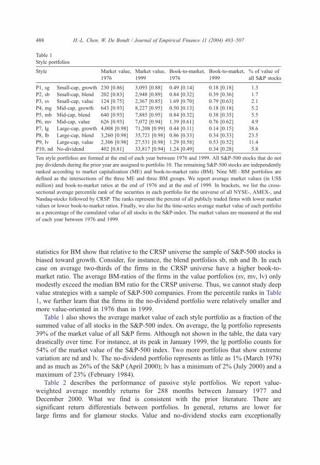
Table 1

Style portfolios

Style Market value,

1976

Market value,

1999

Book-to-market,

1976

Book-to-market,

1999

% of value of

all S&P stocks

P1, sg Small-cap, growth 230 [0.86] 3,093 [0.88] 0.49 [0.14] 0.18 [0.18] 1.3

P2, sb Small-cap, blend 202 [0.83] 2,948 [0.89] 0.84 [0.32] 0.39 [0.36] 1.7

P3, sv Small-cap, value 124 [0.75] 2,367 [0.85] 1.69 [0.70] 0.79 [0.63] 2.1

P4, mg Mid-cap, growth 643 [0.93] 8,227 [0.95] 0.50 [0.13] 0.18 [0.18] 5.2

P5, mb Mid-cap, blend 640 [0.93] 7,885 [0.95] 0.84 [0.32] 0.38 [0.35] 5.5

P6, mv Mid-cap, value 626 [0.93] 7,072 [0.94] 1.39 [0.61] 0.76 [0.62] 4.9

P7, lg Large-cap, growth 4,008 [0.98] 71,208 [0.99] 0.44 [0.11] 0.14 [0.15] 38.6

P8, lb Large-cap, blend 3,260 [0.98] 35,721 [0.98] 0.86 [0.33] 0.34 [0.33] 23.5

P9, lv Large-cap, value 2,306 [0.98] 27,531 [0.98] 1.29 [0.58] 0.53 [0.52] 11.4

P10, nd No-dividend 402 [0.81] 33,817 [0.94] 1.24 [0.49] 0.34 [0.28] 5.8

Ten style portfolios are formed at the end of each year between 1976 and 1999. All S&P-500 stocks that do not

pay dividends during the prior year are assigned to portfolio 10. The remaining S&P-500 stocks are independently

ranked according to market capitalization (ME) and book-to-market ratio (BM). Nine ME–BM portfolios are

defined as the intersections of the three ME and three BM groups. We report average market values (in US$

million) and book-to-market ratios at the end of 1976 and at the end of 1999. In brackets, we list the cross-

sectional average percentile rank of the securities in each portfolio for the universe of all NYSE-, AMEX-, and

Nasdaq-stocks followed by CRSP. The ranks represent the percent of all publicly traded firms with lower market

values or lower book-to-market ratios. Finally, we also list the time-series average market value of each portfolio

as a percentage of the cumulated value of all stocks in the S&P-index. The market values are measured at the end

of each year between 1976 and 1999.


statistics for BM show that relative to the CRSP universe the sample of S&P-500 stocks is

biased toward growth. Consider, for instance, the blend portfolios sb, mb and lb. In each

case on average two-thirds of the firms in the CRSP universe have a higher book-to-

market ratio. The average BM-ratios of the firms in the value portfolios (sv, mv, lv) only

modestly exceed the median BM ratio for the CRSP universe. Thus, we cannot study deep

value strategies with a sample of S&P-500 companies. From the percentile ranks in Table

1, we further learn that the firms in the no-dividend portfolio were relatively smaller and

more value-oriented in 1976 than in 1999.

Table 1 also shows the average market value of each style portfolio as a fraction of the

summed value of all stocks in the S&P-500 index. On average, the lg portfolio represents

39% of the market value of all S&P firms. Although not shown in the table, the data vary

drastically over time. For instance, at its peak in January 1999, the lg portfolio counts for

54% of the market value of the S&P-500 index. Two more portfolios that show extreme

variation are nd and lv. The no-dividend portfolio represents as little as 1% (March 1978)

and as much as 26% of the S&P (April 2000); lv has a minimum of 2% (July 2000) and a

maximum of 23% (February 1984).

Table 2 describes the performance of passive style portfolios. We report value-

weighted average monthly returns for 288 months between January 1977 and

December 2000. What we find is consistent with the prior literature. There are

significant return differentials between portfolios. In general, returns are lower for

large firms and for glamour stocks. Value and no-dividend stocks earn exceptionally

Table 2

The returns of passive style portfolios

Style Value-weighted

return

January February–

December

Standard

deviation

Ave. #

stocks

P1 Small-cap, growth 1.31 (5.29) 1.35 1.31 8.37 (2.81) 28

P2 Small-cap, blend 1.37 (5.14) 1.76 1.34 8.22 (2.40) 42

P3 Small-cap, value 1.59 (5.55) 3.09 1.45 9.65 (2.49) 64

P4 Mid-cap, growth 1.38 (4.93) 1.06 1.41 7.52 (2.29) 44

P5 Mid-cap, blend 1.21 (4.78) 1.30 1.20 6.93 (1.99) 48

P6 Mid-cap, value 1.37 (4.94) 2.70 1.25 7.02 (2.30) 45

P7 Large-cap, growth 1.20 (4.60) 0.97 1.22 6.38 (2.08) 64

P8 Large-cap, blend 1.31 (4.26) 2.01 1.24 6.14 (2.13) 46

P9 Large-cap, value 1.45 (4.78) 2.98 1.31 5.97 (1.97) 28

P10 No-dividend 1.52 (7.27) 4.06 1.29 11.30 (3.48) 47

Ten style portfolios are formed at the end of each year between 1976 and 1999. We study the returns earned by

these portfolios between January 1977 and December 2000 (288 months). For each portfolio, we list time-series

averages of (i) value-weighted average portfolio returns (expressed in percent per month); (ii) portfolio returns for

January; (iii) portfolio returns for February through December (in percent per month); and (iv) monthly cross-

sectional standard deviations of security returns within each portfolio. The corresponding time-series standard

deviations are reported in parentheses. Finally, we list the time-series average number of stocks in each portfolio.


large returns in January. With a return of 1.20% per month (1.22% per month between

February and December), the lg portfolio performs worst of all style portfolios. The sv

portfolio does best. It earns 1.59% per month (1.45% in non-January months). The

average differences in returns between high BM and low BM stocks of similar size

range between minus 1 and plus 28 basis points per month. Along the size dimension,

differences in returns between small and large firms (but with similar BM) are

between 6 and 14 basis points per month. Table 2 also reports the time-series average

cross-sectional standard deviation of returns for the securities in each style portfolio.

This statistic may be thought of as a measure of ‘‘stock-picker’s risk’’. It tells us that,

on average, the range of returns offered by individual stocks in sv or nd is much

wider than for large-cap portfolios.

Fig. 1 shows the variation over time in the annual returns earned since 1977 by the

portfolios of small-cap value, large-cap growth, and no-dividend stocks. Fig. 2 shows the

annual small-cap and value return premia between 1977 and 2000, as well as the annual

return differential between the small-cap value and the large-cap growth portfolios. The

return data are computed in the same way as in Table 2 but annualized. The value premium

is the average return of style portfolios sv, mv, and lv minus the average return of

portfolios sg, mg, and lg. The small-cap premium is the average return of style portfolios

sg, sb, and sv minus the average return of portfolios lg, lb and lv.

The returns reported in Table 2 and shown in Figs. 1 and 2 can be interpreted in the

context of a model that says that the required return for any individual stock at any

given point in time is determined by a limited set of easily observed company

characteristics. A stock’s return is estimated by the return of the style portfolio to

which it belongs. This is because by assumption the returns of firms with comparable

characteristics are driven by the same economic state variables.

Fig. 1. Three style portfolios, 1977–2000.


Evidently, the definition of styles and the number of style portfolios are open to debate.12

There are industry norms as well as econometric considerations that justify our specific

methods. For instance, it is not desirable for a style portfolio to include too few stocks, or for

the cross-sectional standard deviation of returns of each portfolio to vary too much from

month-to-month. (See Table 2 for time-series standard deviations of return variation within

portfolios.) We hope that the partitions capture the basic economic forces that describe the

structure of asset prices.

2. Style momentum

If equity style cycles truly exist, then it may be profitable to buy stocks with in-

favor characteristics and to sell short stocks with characteristics that are out-of-favor.

We explore several such trading strategies. Starting in January 1978, every month, we

rank the 10 style portfolios based on their value-weighted compounded returns over

the previous one, two, three, or four quarters. We go long in past winner stocks (i.e.,

the securities that belong to the one or two style portfolios that performed best) and

short in past loser stocks (i.e., the securities that belong to the one or two portfolios

that performed worst). The subsequent test periods range between one quarter and 3

12 For instance, in 2002, the ‘‘small stock focus’’ column in the Wall Street Journal defines companies as

small-caps if they have a market value below US$1.5 billion. Under this definition, only 17 stocks in the S&P-

500 qualify. David Blitzer, chairman of the S&P-500 index selection committee, says that ‘‘[the committee]

prefers a minimum market cap of $4 billion’’ (Wall Street Journal, April 15, 2002).

Fig. 2. Small-cap and value return premia, 1977–2000.


years. Frequent replications with overlapping test periods increase the power of the

statistical tests. Depending on the length of the test period, the number of replications

varies between 241 and 274. Our calculations of average monthly test period returns

for long and short portfolios give equal weight to each security, to each test period

month, and to each replication.13

Table 3 reports the average return per month of the different buy, sell, and arbitrage

(i.e., buy minus sell) portfolios. It is noteworthy that the returns of the arbitrage

portfolios are always positive. Because the holding periods are partially overlapping,

we adjust the t-statistics for serial correlation and heteroskedasticity. Many of our

findings are statistically significant. The most successful arbitrage strategies select

stocks based on past 12 month returns ( J = 12) and hold for 3, 6, 9 or 12 months

(K = 3, 6, 9, 12). For a ( J = 12; K = 12)-strategy, the profit amounts to 43 basis points

per month (see panel A). The results remind us of the findings of Jegadeesh and

Titman (1993) on price momentum and of Moskowitz and Grinblatt (1999) on industry

momentum. The style momentum profits are strong over intermediate horizons (3 to 12

months) but they are statistically indistinguishable from 0 beyond 1 year. We perform

various robustness checks. For instance, we skip 1 month between the rank and the test

period. In that case, the ( J = 12; K = 12)-strategy earns 41 basis points per month (see

panel B). We also study arbitrage portfolios based on four extreme style portfolios.

13 In other words, our methods closely follow Jegadeesh and Titman (1993) and Moskowitz and Grinblatt

(1999) and allow meaningful comparisons. If a firm leaves the CRSP database after the date of portfolio

formation, then the portfolio returns for the subsequent months of the test period are defined as the arithmetic

average returns for the remaining securities.

Table 3

The returns of style momentum portfolios

Average monthly return during the test period

K = 3 K= 6 K= 9 K= 12 2nd Year 3rd Year

Panel A

Arbitrage portfolio holds two style portfolios

J= 3

1 Winner 1.61 1.58 1.62 1.63 1.47 1.45

1 Loser 1.48 1.48 1.43 1.39 1.37 1.41

Arbitrage 0.13 (0.65) 0.10 (0.70) 0.19 (1.73) 0.23 (2.07) 0.11 (1.00) 0.04 (0.36)

J= 6

1 Winner 1.54 1.65 1.68 1.68 1.41 1.47

1 Loser 1.42 1.48 1.38 1.36 1.37 1.43

Arbitrage 0.12 (0.59) 0.18 (1.21) 0.30 (2.07) 0.32 (2.41) 0.04 (0.36) 0.04 (0.36)

J= 12

1 Winner 1.75 1.80 1.78 1.71 1.48 1.40

1 Loser 1.27 1.30 1.32 1.28 1.39 1.38

Arbitrage 0.48 (2.24) 0.50 (2.63) 0.46 (2.69) 0.43 (2.49) 0.09 (0.61) 0.02 (0.21)

Panel B

Arbitrage portfolio holds two style portfolios. Strategy skips 1 month.

J= 3

1 Winner 1.53 1.62 1.61 1.62 1.45 1.46

1 Loser 1.48 1.44 1.43 1.39 1.35 1.44

Arbitrage 0.05 (0.26) 0.18 (1.31) 0.18 (1.59) 0.23 (2.02) 0.10 (1.00) 0.02 (0.19)

J= 12

1 Winner 1.80 1.85 1.76 1.70 1.48 1.38

1 Loser 1.34 1.33 1.33 1.29 1.41 1.38

Arbitrage 0.45 (2.13) 0.52 (2.82) 0.43 (2.50) 0.41 (2.34) 0.07 (0.43) 0.00 (0.04)

Panel C

Arbitrage portfolio holds four style portfolios

J= 3

2 Winners 1.53 1.54 1.57 1.60 1.50 1.43

2 Losers 1.40 1.42 1.41 1.37 1.41 1.43

Arbitrage 0.14 (0.98) 0.12 (1.01) 0.16 (1.73) 0.23 (2.68) 0.09 (1.11) 0.00 (0.07)

J= 6

2 Winners 1.54 1.55 1.59 1.62 1.48 1.45

2 Losers 1.45 1.46 1.39 1.38 1.40 1.44

Arbitrage 0.08 (0.56) 0.09 (0.80) 0.20 (1.76) 0.24 (2.61) 0.08 (0.79) 0.00 (0.04)

J= 12

2 Winners 1.66 1.65 1.67 1.61 1.56 1.45

2 Losers 1.31 1.30 1.32 1.32 1.43 1.41

Arbitrage 0.35 (2.09) 0.35 (2.45) 0.35 (3.01) 0.29 (2.72) 0.13 (0.87) 0.05 (0.43)

Panel D

Arbitrage portfolio holds four style portfolios. Strategy skips 1 month.

J= 3

2 Winners 1.48 1.56 1.57 1.60 1.48 1.44

2 Losers 1.46 1.44 1.42 1.38 1.41 1.45

Arbitrage 0.03 (0.16) 0.12 (1.04) 0.16 (1.65) 0.22 (2.78) 0.07 (0.84) � 0.01 (� 0.07)


Table 3 (continued )


K= 3 K = 6 K= 9 K = 12 2nd Year 3rd Year

Panel D

Arbitrage portfolio holds four style portfolios. Strategy skips 1 month.

J= 12

2 Winners 1.62 1.68 1.64 1.60 1.56 1.45

2 Losers 1.32 1.32 1.33 1.33 1.44 1.42

Arbitrage 0.30 (1.82) 0.36 (2.59) 0.31 (2.77) 0.27 (2.50) 0.13 (0.84) 0.03 (0.31)

Starting in January 1978, 10 style portfolios are ranked every month by their return performance for the past J

months. J is 3, 6, or 12 months. We buy the top (or the top two) winner style portfolio(s) and we sell the

corresponding loser portfolio(s). The arbitrage portfolios are held for test periods that are K = 3, 6, 9, 12, 24, or 36

months long. Since we employ return data through December 2000, the number of strategy replications is 274,

271, 268, 265, 253, or 241, depending on the length of the test period. Below, we report equally weighted average

returns in percent per month. We also report average monthly returns for the 2nd and 3rd year after portfolio

formation. The t-statistics, listed in parentheses, rely on a Newey–West correction for overlapping observations.

Panels A and C report the test period returns when there is no time gap between the rank and test periods. Panels

B and D report equivalent statistics but skip a month between the rank and test periods.


Then, the ( J = 12; K = 12)-strategy earns either 29 or 27 basis points per month (see

panels C and D).14

We may wonder which investment styles an imaginary trader, who knew the results of

our study before we did, would in fact have followed. Table 4 answers this question. It lists

the best- and worst-performing investment styles and the corresponding cumulative rank

period returns (over 3 or 12 months) at the end of each quarter and at the end of each year

since 1978. It is interesting to note how between the first quarter of 1995 and the second

quarter of 2000 (22 quarters in total) the no dividend portfolio appeared 13 times as the

winner, or how between 1978 and 1981 the large growth portfolio was a frequent loser (9

out of 16 quarters).

In Table 5, we compute the fraction of all monthly strategy replications that a particular

style portfolio was held long or sold short. We report separate statistics for style

momentum arbitrage portfolios that have one or two portfolios on the buy and sell side,

and for 3- and 12-month rank periods. Relative to chance, the styles that are overrepre-

sented are sg, sv, lg, lv, and nd.

Many financial practitioners are locked into delivering unique products (e.g., a small-cap

value portfolio) but rotation managers, by definition, do not have to adhere to one style.

From a rotation perspective, it is key that we assess whether style momentum strategies earn

positive returns after transaction costs. In style momentum strategies, trading occurs for no

less than four distinct reasons: (i) a past winner or loser style no longer produces extreme

performance; (ii) a firm migrates between style portfolios; (iii) a firm joins or leaves the

14 Two recent studies present parallel results. Chen (2003) examines all firms listed on the NYSE, AMEX or

Nasdaq between 1963 and 1997. The securities are sorted into 18 cells. As we may expect from a sample with

many small firms, the magnitudes of the returns earned by the arbitrage portfolios are larger than what we report

here. Lewellen (2002) uses the same CRSP data set as Chen. He shows that well-diversified size (1941–1999)

and book-to-market (1963–1999) portfolios exhibit momentum that is distinct from individual stock momentum.

Table 4

Style momentum portfolios by quarter and year, 1978–2000

W r(w) L r(l) W r(w) L r(l) W r(w) L r(l) W r(w) L r(l) W r(w) L r(l)

1978 1983 1988 1993 1998

q1 sb 8 lg � 2 nd 41 lb 13 sg � 20 sv � 28 nd 15 lv � 3 mv 8 nd � 7

q2 sv 3 lg � 10 nd 17 mg 5 sv 25 lg 1 mv 13 lg � 2 nd 25 mv 9

q3 nd 19 lv 3 sv 16 lg 9 nd 10 lg 3 lv 6 mg � 4 nd 12 sg � 8

q4 sv 15 lg 7 sv 5 nd � 13 lg 4 nd � 7 nd 9 sg � 3 nd � 2 mb � 17

year sb 7 lg � 13 sg 51 lb 9 nd 16 mv � 6 mv 28 lg 4 lg 36 sg 16

1979 1984 1989 1994 1999

q1 lg � 3 sv � 15 mv 4 nd � 4 lv 5 mv � 1 sb 8 mv � 2 nd 32 mv 9

q2 sv 16 lg 3 lv 6 sg � 11 mv 12 sb 5 sv 2 lv � 7 nd 17 mb � 3

q3 sv 7 lg � 1 sg 0 mv � 11 sv 11 lv 6 mv 4 nd � 5 sv 22 nd 5

q4 nd 16 lg 4 mv 13 sv 5 mg 12 sv 8 sv 11 lb 2 nd 1 mb � 15

year nd 21 lv 1 sv 44 mg 10 sv 35 nd 7 lv 29 sg � 3 nd 81 sb 2

1980 1985 1990 1995 2000

q1 nd 9 sv � 3 sb 8 nd 0 lg 5 nd � 7 nd 2 sg � 4 nd 36 mv � 5

q2 lb 0 sb � 14 mb 13 nd 5 lv 1 sg � 7 mg 13 nd 7 nd 8 sv � 9

q3 mg 24 lg 10 lv 10 sv 2 lg 12 sv 1 nd 20 sg 4 sg 11 lv � 13

q4 nd 35 lv 4 sb 1 nd � 7 lb � 6 nd � 30 lv 12 sg 3 lv 34 nd � 10

year nd 50 lg 6 lv 17 sv � 2 lg 40 sb 21 sv 7 sb � 7 nd 69 mv � 9

1981 1986 1991 1996

q1 lb 16 lv 1 lg 22 lv 13 mg 12 lb 6 lb 8 sg � 2

q2 sv 18 lg � 4 sb 21 nd 11 sv 26 lb 8 mg 10 mv 3

q3 lv 7 lg � 6 lg 9 sv � 4 sv 7 nd � 4 nd 8 sg 0

q4 lv � 4 sg � 18 lv 0 mg � 15 mv 7 lv 0 lb 4 sv 1

year nd 54 lv 13 sg 41 nd 24 lg 4 mv � 21 lv 41 sg 19

1982 1987 1992 1997

q1 sg 10 lv 2 mg 9 sb 2 lg 14 lv 0 lv 11 sb 2

q2 sg 0 nd � 12 nd 34 mv 17 sv 12 lg � 6 lb 5 sg � 1

q3 sb 5 nd � 8 sv 9 sb � 3 lv 8 nd � 5 nd 25 mv 10

q4 sg 19 nd 5 sv 16 lv 2 mg 8 lv � 8 nd 16 lg 3

year lv 19 lb � 12 mb 27 nd 5 sv 54 lb 17 nd 27 sg 11

At the beginning of each quarter (year) we rank 10 style portfolios by their returns over the previous quarter

(year). W denotes the most extreme winner portfolio; L, the most extreme loser portfolio. r(w) is the quarterly

(annual) rank period return, in percent, of the winner portfolio; r(l) is the return of the loser portfolio. The 10 style

portfolios are small-cap growth (sg), small-cap blend (sb), small-cap value (sv), mid-cap growth (mg), mid-cap

blend (mb), mid-cap value (mv), large-cap growth (lg), larg-cap blend (lb), large-cap value (lv), and no-dividend

(nd).


S&P-500 index; and (iv) a firm performs differently from other firms within the same style

portfolio and the portfolio requires rebalansing. Without any doubt, the transaction costs

associated with style momentum strategies are non-trivial.15 We conjecture therefore that

15 Note that Tables 4 and 5 illustrate the amount of trading that is required for the first reason on the list only.

However, two factors that moderate trading costs are that (i) S&P-500 firms are very liquid stocks, and (ii) we

switch between no more than 10 style portfolios.

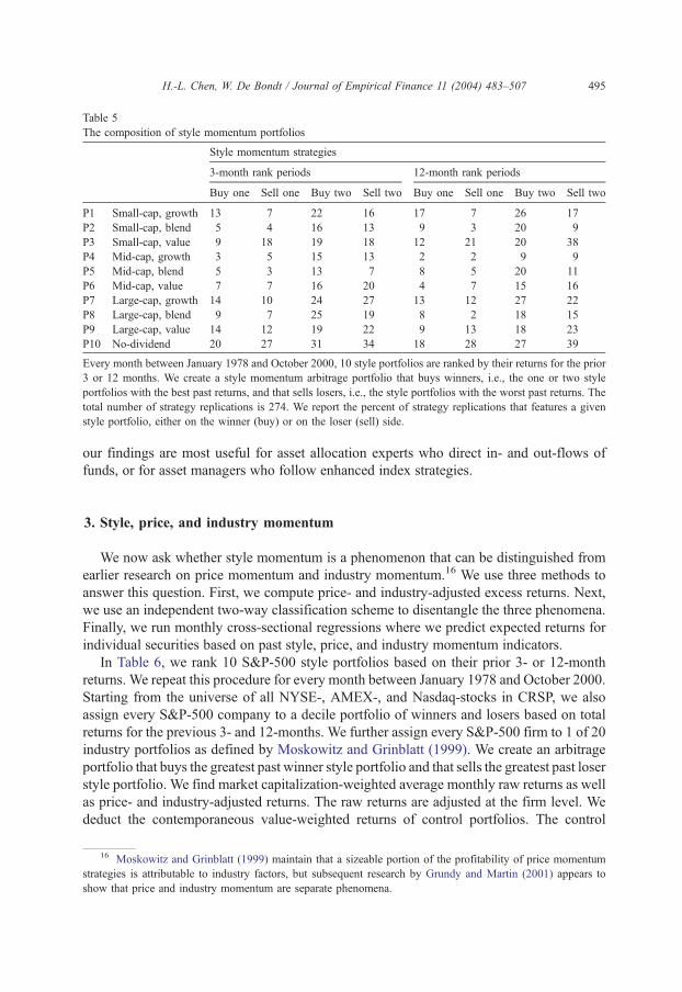
Table 5

The composition of style momentum portfolios

Style momentum strategies

3-month rank periods 12-month rank periods

Buy one Sell one Buy two Sell two Buy one Sell one Buy two Sell two

P1 Small-cap, growth 13 7 22 16 17 7 26 17

P2 Small-cap, blend 5 4 16 13 9 3 20 9

P3 Small-cap, value 9 18 19 18 12 21 20 38

P4 Mid-cap, growth 3 5 15 13 2 2 9 9

P5 Mid-cap, blend 5 3 13 7 8 5 20 11

P6 Mid-cap, value 7 7 16 20 4 7 15 16

P7 Large-cap, growth 14 10 24 27 13 12 27 22

P8 Large-cap, blend 9 7 25 19 8 2 18 15

P9 Large-cap, value 14 12 19 22 9 13 18 23

P10 No-dividend 20 27 31 34 18 28 27 39

Every month between January 1978 and October 2000, 10 style portfolios are ranked by their returns for the prior

3 or 12 months. We create a style momentum arbitrage portfolio that buys winners, i.e., the one or two style

portfolios with the best past returns, and that sells losers, i.e., the style portfolios with the worst past returns. The

total number of strategy replications is 274. We report the percent of strategy replications that features a given

style portfolio, either on the winner (buy) or on the loser (sell) side.


our findings are most useful for asset allocation experts who direct in- and out-flows of

funds, or for asset managers who follow enhanced index strategies.

3. Style, price, and industry momentum

We now ask whether style momentum is a phenomenon that can be distinguished from

earlier research on price momentum and industry momentum.16 We use three methods to

answer this question. First, we compute price- and industry-adjusted excess returns. Next,

we use an independent two-way classification scheme to disentangle the three phenomena.

Finally, we run monthly cross-sectional regressions where we predict expected returns for

individual securities based on past style, price, and industry momentum indicators.

In Table 6, we rank 10 S&P-500 style portfolios based on their prior 3- or 12-month

returns. We repeat this procedure for every month between January 1978 and October 2000.

Starting from the universe of all NYSE-, AMEX-, and Nasdaq-stocks in CRSP, we also

assign every S&P-500 company to a decile portfolio of winners and losers based on total

returns for the previous 3- and 12-months. We further assign every S&P-500 firm to 1 of 20

industry portfolios as defined by Moskowitz and Grinblatt (1999). We create an arbitrage

portfolio that buys the greatest past winner style portfolio and that sells the greatest past loser

style portfolio. We find market capitalization-weighted average monthly raw returns as well

as price- and industry-adjusted returns. The raw returns are adjusted at the firm level. We

deduct the contemporaneous value-weighted returns of control portfolios. The control

16 Moskowitz and Grinblatt (1999) maintain that a sizeable portion of the profitability of price momentum

strategies is attributable to industry factors, but subsequent research by Grundy and Martin (2001) appears to

show that price and industry momentum are separate phenomena.

Table 6

Raw returns vs. style-, price-, and industry-adjusted returns

Panel A: 3-month rank periods


K= 3 K= 6 K= 9 K= 12 2nd Year 3rd Year

Style momentum

Raw 0.15

[0.62]

0.10

[0.53]

0.15

[1.00]

0.28

[1.75]

0.20

[1.46]

0.09

[0.73]

Price-adjusted 0.01

[0.04]

0.05

[0.35]

0.18

[1.32]

0.25

[1.90]

0.21

[1.62]

0.07

[0.63]

Industry-adjusted 0.11

[0.66]

0.12

[0.98]

0.17

[1.62]

0.24

[2.22]

0.23

[1.97]

0.05

[0.58]

Price momentum

Raw � 0.05

[� 0.21]

0.01

[0.02]

0.21

[1.35]

0.37

[2.76]

� 0.12

[� 0.87]

� 0.22

[� 1.46]

Industry-adjusted � 0.17

[� 1.00]

� 0.13

[� 0.94]

0.06

[0.61]

0.18

[2.09]

� 0.03

[� 0.26]

� 0.13

[� 1.30]

Style-adjusted � 0.04

[� 0.22]

0.03

[0.19]

0.23

[1.78]

0.32

[2.92]

� 0.14

[� 1.13]

� 0.21

[� 1.59]

Industry momentum

Raw � 0.14

[� 0.60]

0.15

[0.69]

0.24

[1.37]

0.30

[2.14]

� 0.13

[� 1.16]

� 0.15

[� 0.87]

Price-adjusted � 0.21

[� 1.06]

0.11

[0.58]

0.23

[1.52]

0.27

[2.12]

� 0.13

[� 1.21]

� 0.23

[� 1.29]

Style-adjusted � 0.07

[� 0.37]

0.20

[1.14]

0.26

[1.81]

0.29

[2.32]

� 0.16

[� 1.30]

� 0.13

[� 0.82]

Panel B: 12-month rank periods

Style momentum

Raw 0.61

[2.16]

0.65

[2.50]

0.64

[2.76]

0.65

[2.81]

0.22

[1.07]

� 0.02

[� 0.12]

Price-adjusted 0.47

[2.33]

0.55

[2.90]

0.55

[3.14]

0.54

[3.00]

0.17

[0.88]

� 0.10

[� 0.55]


[2.74]

0.57

[3.46]

0.58

[3.58]

0.56

[3.17]

0.22

[1.18]

� 0.11

[� 0.95]

Price momentum

Raw 0.73

[2.18]

0.69

[2.41]

0.69

[2.98]

0.55

[2.87]

� 0.24

[� 0.92]

� 0.35

[� 1.50]


[1.70]

0.43

[2.32]

0.44

[2.92]

0.35

[2.58]

� 0.03

[� 0.15]

� 0.29

[� 2.24]

Style-adjusted 0.79

[3.05]

0.67

[3.05]

0.64

[3.53]

0.51

[3.25]

� 0.24

[� 1.12]

� 0.31

[� 1.74]

Industry momentum

Raw 0.50

[1.49]

0.57

[1.89]

0.46

[1.73]

0.37

[1.65]

� 0.13

[� 0.75]

� 0.07

[� 0.25]

Price-adjusted 0.41

[1.64]

0.43

[1.80]

0.29

[1.34]

0.20

[1.04]

� 0.23

[� 1.22]

� 0.28

[� 1.01]





K = 3 K = 6 K= 9 K = 12 2nd Year 3rd Year

Industry momentum

Style-adjusted 0.53

[1.93]

0.57

[2.29]

0.45

[1.94]

0.34

[1.66]

� 0.17

[� 1.06]

� 0.05

[� 0.19]

We study three momentum strategies and their interaction. Every month, starting in January 1978, we rank the

companies in the S&P-500 index into 10 portfolios based on (1) the past 3- or 12-month returns of the style portfolios

to which they belong, (2) their own past 3- or 12-month returns, and (3) the past 3- or 12-month returns of the

industry portfolios to which they belong.We employ return data through the end of the year 2000. Depending on the

length of the test period (K= 3, 6, 9, 12, 24, or 36 months), the number of replications is 274, 271, 268, 265, 253, or

241. We create arbitrage portfolios that buy the greatest past winners and that sell the greatest past losers. The style

momentum strategy assigns S&P-stocks to portfolios as explained in Table 1. The price momentum strategy buys

the 50 biggest S&P-winners and sells the 50 biggest S&P-losers. The industry momentum strategy only buys (sells)

S&P-stocks that belong to the two industries that performed the best (the worst) during the rank period. (In this case,

the universe of all NYSE-, AMEX-, and Nasdaq-stocks is used to rank industries. Our method and definition of

industries follows Moskowitz and Grinblatt, 1999.) We report value-weighted average raw returns during the test

period, as well as style-, price-, or industry-adjusted returns, all expressed in percent per month. (The value weights

use the market capitalization figures for the last trading day of the previous month. The value-weighted returns are

equally weighted across replications, across months, and across winners and losers.) The raw returns are adjusted at

the firm level. We deduct the contemporaneous value-weighted returns of control portfolios. The control portfolios

are either the matching price momentum or industry portfolios, both for the universe of all NYSE-, AMEX-, and

Nasdaq-stocks, or the matching style portfolio for S&P-companies. We find the match with data for the rank period.

Panel A lists the results for ranks based on the past 3 months of returns; panel B, for ranks based on the past 12

months. The t-statistics, listed in brackets, rely on a Newey–West correction for overlapping observations.


portfolios are either the matching price momentum or industry portfolios defined immedi-

ately above. We find the correct match with data for the rank period. Panel A lists the results

for style ranks based on the past 3 months of returns; panel B, for ranks based on the past 12

months. The arbitrage portfolio (winnersminus losers) is held for horizons of 3 to 36months.

The results in Table 6 imply that it is difficult to disregard style momentum, especially for

ranks based on the past 12 months. The reason is that the price- and industry-adjusted style

momentum arbitrage profits are of similar magnitude to the raw profits. For example, over 1

year, a style arbitrage portfolio earns a raw return of 65 basis points per month, it earns 54

basis points with an adjustment for price momentum, and it earns 56 basis points with an

adjustment for industry momentum. As before, these profits do not persist during the second

and third year after portfolio formation.17

One interpretation of the findings is that the price and industry momentum phenomenon

may not apply to S&P-500 firms and that for this reason return adjustments are pointless.

This argument is false, as Table 6 shows. The three momentum strategies do not subsume

each other. We study price momentum strategies that buy the 50 biggest S&P-winners and

sell the 50 biggest S&P-losers. We also examine industry momentum strategies that buy

(sell) S&P-stocks that belong to the 2 of 20 industries that performed the best (the worst)

during the rank period. (As before, the CRSP universe is used to rank industries.) In both

17 That the arbitrage profits are slightly different from what was discussed in Section 2 is due to the fact that

the returns listed in Table 3 are equally weighted while the returns in Table 6 are value-weighted.


cases, we estimate raw and adjusted returns in a comparable way to what we did for style

momentum strategies. For 3-month rank periods, price and industry momentum become

statistically significant in arbitrage portfolios over 12-month horizons. This is similar to

what is seen for style momentum. However, the profits of price and industry momentum

strategies are slightly larger (see panel A). The opposite is true for 12-month rank periods

Table 7

The returns of price and industry momentum portfolios that vary in style momentum


K= 3 K = 6 K = 9 K= 12 2nd Year 3rd Year


(P1,S1) 1.45 1.51 1.60 1.67 1.45 1.45

(P1,S3) 1.29 1.39 1.46 1.48 1.45 1.38

(P1,S1)– (P1,S3) 0.16 (1.17) 0.12 (1.14) 0.13 (1.58) 0.18 (2.32) � 0.00 (� 0.01) 0.08 (1.12)

(P2,S1) 1.51 1.48 1.47 1.50 1.50 1.41

(P2,S3) 1.38 1.44 1.44 1.43 1.39 1.48

(P2,S1)– (P2,S3) 0.13 (1.24) 0.04 (0.47) 0.03 (0.51) 0.07 (1.23) 0.11 (1.77) � 0.07 (� 0.96)

(P3,S1) 1.67 1.58 1.49 1.46 1.56 1.47

(P3,S3) 1.45 1.41 1.38 1.31 1.46 1.49

(P3,S1)– (P3,S3) 0.22 (1.68) 0.17 (1.69) 0.11 (1.30) 0.16 (2.26) 0.10 (1.03) � 0.02 (� 0.24)

(I1,S1) 1.53 1.53 1.59 1.62 1.41 1.42

(I1,S3) 1.36 1.40 1.48 1.47 1.33 1.33

(I1,S1)– (I1,S3) 0.17 (1.11) 0.13 (1.03) 0.10 (1.17) 0.15 (1.64) 0.08 (0.92) 0.10 (1.09)

(I2,S1) 1.45 1.49 1.52 1.56 1.49 1.44

(I2,S3) 1.43 1.47 1.44 1.40 1.39 1.47

(I2,S1)– (I2,S3) 0.02 (0.17) 0.02 (0.17) 0.08 (0.89) 0.16 (2.06) 0.10 (1.32) � 0.03 (� 0.50)

(I3,S1) 1.44 1.41 1.39 1.41 1.56 1.42

(I3,S3) 1.32 1.32 1.31 1.29 1.51 1.49

(I3,S1)– (I3,S3) 0.12 (0.86) 0.09 (0.90) 0.08 (1.09) 0.13 (2.23) 0.04 (0.66) � 0.06 (� 0.95)


(P1,S1) 1.84 1.83 1.81 1.74 1.51 1.48

(P1,S3) 1.57 1.52 1.46 1.42 1.28 1.34

(P1,S1)– (P1,S3) 0.27 (1.66) 0.31 (2.18) 0.35 (3.00) 0.33 (2.94) 0.23 (1.88) 0.15 (1.45)

(P2,S1) 1.53 1.54 1.51 1.51 1.50 1.47

(P2,S3) 1.35 1.36 1.36 1.350 1.38 1.42

(P2,S1)– (P2,S3) 0.18 (1.52) 0.18 (1.77) 0.15 (1.83) 0.16 (1.86) 0.12 (1.17) 0.05 (0.42)

(P3,S1) 1.47 1.50 1.51 1.51 1.62 1.51

(P3,S3) 1.22 1.25 1.25 1.30 1.50 1.44

(P3,S1)– (P3,S3) 0.25 (1.81) 0.25 (2.08) 0.26 (2.54) 0.21 (2.09) 0.12 (0.68) 0.08 (0.65)

(I1,S1) 1.69 1.68 1.66 1.63 1.46 1.50

(I1,S3) 1.50 1.47 1.45 1.38 1.21 1.32

(I1,S1)– (I1,S3) 0.18 (1.05) 0.21 (1.37) 0.21 (1.58) 0.25 (1.95) 0.24 (1.86) 0.19 (1.44)

(I2,S1) 1.67 1.67 1.65 1.60 1.59 1.43

(I2,S3) 1.38 1.41 1.37 1.34 1.40 1.39

(I2,S1)– (I2,S3) 0.28 (2.24) 0.26 (2.32) 0.29 (2.87) 0.26 (2.37) 0.19 (1.52) 0.04 (0.39)

(I3,S1) 1.42 1.42 1.41 1.44 1.60 1.47

(I3,S3) 1.11 1.21 1.24 1.39 1.52 1.45

(I3,S1)– (I3,S3) 0.31 (2.04) 0.21 (1.65) 0.17 (1.48) 0.11 (1.02) 0.08 (0.67) 0.03 (0.22)


(see panel B). In this case, style momentum strategies perform best—with or without

return adjustments. Industry momentum strategies perform worst.

Table 7 further examines the interaction of style, price and industry momentum.

However, we address the issue in another way. We use an independent two-way classifi-

cation scheme. (This method avoids the sorting problems discussed by Berk, 2000.) Every

month, nine S&P-500 portfolios are formed based on style, price, and industry momentum

ranks. First, 10 style portfolios are ranked either by 3- or 12-month rank period returns. Style

portfolios in the top three are labeled #1 (winners) while stocks in the bottom three are

labeled #3 (losers). Portfolios in the middle are labeled #2. Next, all S&P-500 stocks,

depending on their prior 3- or 12-month performance, are labeled #1 (winners; the top third),

#3 (losers; the bottom third), or #2 (in between). Finally, 20 industry portfolios are ranked by

prior 3- or 12-month performance. Industry portfolios in the top seven are labeled #1

(winners) while portfolios in the bottom seven are labeled #3 (losers). Portfolios in between

are labeled #2. The industry portfolios are defined in the usual way (Moskowitz and

Grinblatt, 1999).

In pairwise comparisons between price- and style-momentum (P,S-portfolios), and

between industry- and style-momentum (I,S-portfolios), every S&P-500 stock is assigned

to one of nine portfolios. In panel A of Table 7, we report equally weighted average monthly

returns for P,S- and I,S-portfolios during the test period when the ranks are based on 3-month

returns. Sorted by price momentum, the best past investment styles continue for the next 12

months (K = 12) to beat the worst past styles by between 7 and 18 basis points per month.

Sorted by industry momentum, the best past investment styles continue to beat the worst past

styles by between 13 and 16 basis points per month. Panel B shows that the usual

performance gap between extreme investment styles is even larger for portfolios ranked

by 12-month price or industry momentum.

Table 8 lists the results of our third and final attempt to disentangle style, price and

industry momentum. This time, we run monthly cross-sectional multivariate regressions

between test period returns for individual S&P-500 firms and their monthly style, price,

and industry momentum indicators. To determine the price and industry indicators, we use

the CRSP universe. We first assign all firms to decile portfolios of winners and losers. The

Notes to Table 7:

Every month, starting in January 1978, we form groups of stocks based on rank indicators for style (S), price (P),

and industry momentum (I). In the case of S, 10 S&P-500 style portfolios are ranked by their returns over the

prior 3 or 12 months. The top three style portfolios are labeled #1 (winners). The bottom three are labeled #3

(losers). Portfolios in the middle are labeled #2. In the case of P, all S&P-500 stocks, depending on their

individual prior 3- or 12-month returns, are labeled either #1 (winners; the top 33%), #3 (losers; the bottom 33%),

or #2 (in between). In the case of I, 20 industry portfolios defined by Moskowitz and Grinblatt (1999) over the

universe of all NYSE-, AMEX-, and Nasdaq-listed stocks are ranked by their prior 3- or 12-month returns. The

top seven industry portfolios are labeled #1 (winners). The bottom seven are labeled #3 (losers). Portfolios in the

middle are labeled #2. In pairwise comparisons between P and S, and I and S, every S&P-500 stock is assigned to

one of nine portfolios defined as the intersections of S, P, and I. (By construction, the nine portfolio do not hold

the same number of securities.) In panel A, we report equally weighted average returns during the test period for

(P,S) and (I,S) portfolios when the ranks are based on 3-month returns. In panel B, we report similar statistics but

the ranks are based on 12-month returns. We use return data through December 2000. The test periods are 3, 6, 9,

or 12 months. We also list average monthly returns for the 2nd and 3rd year after portfolio formation. The t-

statistics (in parentheses) use a Newey–West correction for overlapping observations.

Table 8

Momentum and the cross-section of equity returns

3-month rank periods 6-month rank periods 12-month rank periods

PM IM SM PM IM SM PM IM SM

3-month

test returns

� 0.12

(� 2.08)

0.04

(0.92)

0.06

(1.29)

� 0.05

(� 0.77)

0.03

(0.54)

0.06

(1.11)

0.13

(1.81)

0.10

(1.71)

0.11

(1.99)

6-month

test returns

� 0.11

(� 1.32)

0.11

(1.42)

0.07

(1.04)

0.06

(0.56)

0.17

(1.76)

0.09

(1.04)

0.30

(2.07)

0.13

(1.33)

0.24

(2.60)

12-month

test returns

0.32

(2.55)

0.26

(2.40)

0.23

(2.18)

0.51

(2.68)

0.28

(2.12)

0.26

(2.08)

0.52

(1.98)

0.10

(0.60)

0.48

(2.85)

24-month

test returns

0.35

(1.99)

� 0.04

(� 0.19)

0.38

(1.88)

0.50

(1.92)

� 0.13

(� 0.52)

0.46

(1.72)

0.57

(1.56)

� 0.55

(� 1.95)

0.90

(2.09)

Starting in January 1978, we run monthly cross-sectional multivariate regressions between test period returns for

S&P-500 companies and price, industry, and style momentum indicators. We use return data through the end of the

year 2000. Below,we list time-series average estimated regression coefficients. The t-statistics, listed in parentheses,

rely on a Newey–West correction for overlapping observations. For the price and industry indicators, we use the

universe of all NYSE-, AMEX-, and Nasdaq-stocks followed by CRSP.We assign all companies to decile portfolios

of winners and losers. The portfolios are based on rank period returns over the previous 3, 6, and 12months. Extreme

losers are in decile 1; extreme winners in decile 10. The price momentum indicator (PM) is the decile to which the

S&P-company belongs. We further create monthly ranks of 20 industry portfolios defined by Moskowitz and

Grinblatt (1999). The ranks are based on prior 3-, 6-, and 12-month industry returns. The two industries with the

lowest rank receive a score of one, the next two industries receive a score of two, and so on. Every S&P-company

receives the score of the industry (IM) to which it belongs. Finally, we compute style momentum indicators (SM) by

ranking 10 style portfolios based on their 3-, 6-, and 12-month returns. The style portfolio with the worst past

performance receives a score of 1; the style portfolio with the best performance, a score of 10. Every S&P-company

receives the score of the style portfolio to which it belongs. Raw buy-and-hold test period returns for individual

securities, calculated over 3, 6, 12 and 24 months, are the dependent variables.


portfolios are based on rank period returns over 3, 6, or 12 months. Extreme losers are in

decile 1; extreme winners in decile 10. The price momentum indicator (PM) is the decile to

which the S&P-company belongs. Next, we construct ranks for 20 industry portfolios

based on their prior 3-, 6- or 12-month returns. The two industries with the lowest rank

receive a score of one, the next two industries receive a score of two, and so on. Every

S&P-firm receives the score of the industry (IM) to which it belongs. Finally, we compute

style momentum indicators (SM) by ranking 10 style portfolios based on their 3-, 6-, and

12-month returns. The style portfolio with the worst past performance has a score of one;

the style portfolio with the best performance, a score of 10. Every S&P-company receives

the score of the style portfolio to which it belongs. We run regressions with raw buy-and-

hold test period returns—defined over 3, 6, 12, or 24 months—as the dependent variables.

Following the tradition of Fama and MacBeth, Table 8 lists the time-series averages of the

regression estimates.of the regression estimates.

The tests leave little doubt that style momentum is a determinant of S&P-equity returns

that survives the inclusion of price and industry momentum indicator variables. We

estimate the average difference in expected annual return between a firm that based on its

performance over the past year belongs to style decile 1 and a second company that

belongs to style decile 10. It is (0.48)*(9) = 4.32%. The results are similar for companies

that differ in past price momentum (4.68%). Yet, an equivalent calculation for firms that

vary in past industry momentum yields a statistically insignificant return difference of just

Table 9

The risk of style momentum portfolios

Intercept RMRF SMB HML R2


Winner 0.19 (1.30) 1.13 (31.36) 0.33 (6.22) 0.16 (3.26) 0.82

Loser � 0.12 (� 0.69) 1.14 (26.19) 0.11 (1.71) 0.51 (8.42) 0.72

Arbitrage 0.31 (1.31) � 0.01 (� 0.12) 0.22 (2.54) � 0.34 (� 4.21) 0.14


Winner 0.22 (1.52) 1.13 (31.52) 0.38 (7.13) 0.18 (3.56) 0.83

Loser � 0.22 (� 1.32) 1.14 (27.91) � 0.00 (� 0.04) 0.46 (8.15) 0.74

Arbitrage 0.44 (1.87) � 0.01 (� 0.08) 0.38 (4.44) � 0.28 (� 3.52) 0.17

Ten style portfolios within the S&P-500 index are ranked by their prior 3- or 12-month returns. We buy the

greatest past winner portfolio and we sell the greatest past loser portfolio. The winner, loser, and arbitrage

portfolios are held for 3 or 12 months at which time the strategy is repeated. Thus, the test periods (as well

as the rank periods) are non-overlapping. We estimate regressions with monthly observations between January

1978 and December 2000. In each case, the dependent variable is the equally weighted average portfolio

return during the test period in excess of the 1-month Treasury bill rate. The explanatory variables are the

contemporaneous monthly returns of the three factors studied by Fama and French (1996). The value-

weighted CRSP return index for all NYSE-, AMEX-, and Nasdaq-listed firms is our proxy for the market

return. The regression R2 is adjusted for degrees of freedom. As usual, t-statistics are shown in parentheses.


0.90%. Furthermore, the explanatory power of style momentum extends to 2-year test

returns. This is not the case for price momentum. Industry momentum contributes

negatively during the second year so that, over 24 months, stocks that belong to past

winner industries underperform past losers by 4.95%.

4. The risk and return of style momentum

We now briefly examine the risk of style momentum strategies. This is a weighty topic.

What we present is the first round of an on-going investigation. Previous theoretical and

empirical research by Conrad and Kaul (1998), Johnson (2002), Lewellen (2002), and

others contends that rational cross-sectional and time-series variation in risk is a plausible

explanation of price momentum.18 On the other hand, Hong et al. (2000) and Lee and

Swaminathan (2000) observe that the profitability of momentum strategies is related to the

speed with which information diffuses into prices, and De Bondt and Thaler (1985) and

Jegadeesh and Titman (2001) report that medium-horizon price momentum is typically

followed by price reversals. These findings indicate that the profits of momentum

investing arise from a delayed overreaction to news.

Table 9 characterizes the style momentum portfolios studied in Tables 1–5 and

presents risk-adjusted returns. At regular intervals, the already familiar style portfolios

are sorted by their prior 3- or 12-month returns. However, in this case, the winner,

18 Liew and Vassalou (2000) use 1978–1996 data for 10 countries to show that the profitability of the

Fama–French size and book-to-market factors is linked to future growth in GDP. However, similar reasoning,

Liew and Vassalou find, is invalid for price momentum. Fama and French (1996) also report that risk adjustments

do not explain price momentum but tend to accentuate the anomaly.

Table 10

The returns of style momentum portfolios during selected periods



K = 3 K= 6 K= 9 K= 12 K = 3 K= 6 K = 9 K= 12

Panel A

1978–1985 (n= 96)

Winner 2.03 1.93 1.94 1.87 2.08 2.12 2.03 1.91

Loser 1.73 1.66 1.67 1.67 1.46 1.56 1.54 1.49

Arbitrage 0.30

(0.91)

0.27

(1.20)

0.27

(1.86)

0.21

(1.75)

0.62

(1.99)

0.57

(2.56)

0.49

(2.22)

0.42

(1.76)

1986–1993 (n= 96)

Winner 1.19 1.08 1.18 1.23 1.57 1.56 1.46 1.36

Loser 1.30 1.36 1.30 1.21 1.43 1.36 1.39 1.35

Arbitrage � 0.11

(� 0.43)

� 0.28

(� 1.60)

� 0.12

(� 0.77)

0.01

(0.09)

0.14

(0.45)

0.20

(0.70)

0.07

(0.30)

0.01

(0.04)

1994–2000 (n= 82 or less)

Winner 1.60 1.75 1.76 1.83 1.58 1.69 1.87 1.91

Loser 1.39 1.39 1.29 1.28 0.88 0.91 0.94 0.93

Arbitrage 0.22

(0.46)

0.37

(1.11)

0.47

(2.09)

0.55

(1.94)

0.70

(1.46)

0.78

(1.70)

0.93

(2.40)

0.98

(2.63)

Panel B

After high cross-sectional dispersion

Winner 1.93 2.02 1.52 1.73 1.34 1.85 1.76 1.58

Loser 1.25 1.54 1.28 1.20 0.68 1.05 0.92 0.74

Arbitrage 0.69

(1.30)

0.48

(1.46)

0.24

(0.95)

0.53

(2.02)

0.67

(1.27)

0.80

(2.13)

0.85

(2.53)

0.84

(3.11)

After medium cross-sectional dispersion

Winner 1.37 1.49 1.63 1.60 1.70 1.81 1.86 1.79

Loser 1.37 1.49 1.45 1.45 1.24 1.50 1.57 1.48

Arbitrage 0.00

(0.02)

0.00

(0.00)

0.18

(1.74)

0.15

(1.71)

0.42

(2.49)

0.30

(2.88)

0.29

(3.39)

0.31

(3.94)

After low cross-sectional dispersion

Winner 1.99 1.41 1.69 1.61 2.45 1.74 1.55 1.60

Loser 2.04 1.37 1.52 1.40 1.99 0.93 0.91 1.18

Arbitrage � 0.04

(� 0.18)

0.05

(0.31)

0.17

(1.42)

0.21

(1.88)

0.45

(2.20)

0.80

(4.99)

0.64

(4.63)

0.42

(4.00)

Panel C

After bull markets

Winner 2.03 1.83 1.54 1.58 0.04 0.91 1.13 1.00

Loser 1.25 1.40 1.17 1.15 � 0.44 0.48 0.74 0.66

Arbitrage 0.77

(2.08)

0.43

(2.24)

0.37

(2.40)

0.44

(2.50)

0.48

(1.59)

0.43

(1.83)

0.39

(2.26)

0.34

(2.09)

After normal markets

Winner 1.02 1.18 1.43 1.44 2.09 1.87 1.79 1.73

Loser 0.96 1.12 1.23 1.19 1.58 1.29 1.19 1.17

Arbitrage 0.06

(0.30)

0.05

(0.43)

0.19

(1.84)

0.25

(2.63)

0.51

(2.44)

0.58

(4.15)

0.60

(4.85)

0.57

(5.71)





K= 3 K= 6 K= 9 K = 12 K= 3 K = 6 K= 9 K= 12

After bear markets

Winner 2.93 2.52 2.28 2.23 2.44 2.48 2.40 2.35

Loser 3.23 2.59 2.29 2.26 2.08 2.14 2.25 2.22

Arbitrage � 0.29

(� 0.74)

� 0.07

(� 0.25)

� 0.01

(� 0.07)

� 0.03

(� 0.16)

0.37

(1.27)

0.34

(1.85)

0.15

(1.08)

0.13

(1.00)

Every month, starting in January 1978, 10 S&P-500 style portfolios are ranked by their prior 3- or 12-month

returns. We buy the style portfolio with the best returns over the rank period and we sell the portfolio with the

worst returns. The arbitrage portfolio is held for K= 3, 6, 9, or 12 months. We have data through December 2000.

Thus, the number of replications (n) for the full period is 274, 271, 268, or 265. We report equally weighted

average test period returns, expressed in percent per month. In panel A, we study three sub-periods. (Note that, for

1994–2000, n falls as K rises.) In panel B, we sort replications by the difference in rank-period returns between

the best and worst performing style portfolios; in panel C, by the rank period return on the value-weighted CRSP

index of NYSE-, AMEX-, and Nasdaq-listed firms. The test period returns are shown for periods that follow 3- or

12-month stretches of time with high cross-sectional dispersion in performance (the top 20% of replications), with

medium dispersion (the middle 60%), and with low dispersion (the bottom 20%) as well as for periods that follow

bull markets (the 20% of replications with the best market performance), normal markets (the middle 60%), and

bear markets (the 20% with the worst performance). As usual, t-statistics are listed in parentheses.


loser, and arbitrage portfolios are held for 3 or 12 months before the strategy is

repeated. Thus, the rank and the test periods do not overlap. We estimate time-series

regressions with monthly observations between January 1978 and December 2000. The

dependent variables are equally weighted average test period returns in excess of the 1-

month Treasury bill rate. The explanatory variables are the contemporaneous monthly

returns of the three factors (the market factor, SMB and HML) proposed by Fama and

French (1996). The value-weighted CRSP return for all NYSE-, AMEX-, and Nasdaq-

firms is our proxy for the market return.

Table 9 lists a Fama–French alpha of 31 basis points per month for a style momentum

arbitrage portfolio that is updated quarterly and an alpha of 44 basis points for an arbitrage

portfolio that is updated annually. Only the second alpha is statistically significant. Both

portfolios are market-neutral. Their return dynamics mirror to some extent what is typical

for small, growth-oriented companies. The factor sensitivity to SMB is mostly caused by

stocks that reflect past winner investment styles; the sensitivity to HML is produced by

stocks that typify past loser styles.

A different way to judge the risk/return characteristics of style momentum strategies is to

study subperiods. Chordia and Shivakumar (2002) find that price momentum strategies do

not earn profits during recessions. Jensen et al. (1998) find that the size and value premia in

U.S. stocks are predictably higher in an expansionary monetary policy environment.19

19 One interpretation of these results is that small firms often do not have as much collateral as large firms

and have a lesser ability to raise external funds. Therefore, small firms are more adversely affected by high

interest rates. Gertler and Gilchrist (1994) describe the dissimilar responses of small and large manufacturing

firms to tight credit market conditions, e.g., in the financing of inventory. Perez-Quiros and Timmermann (2000)

show that the risk and return of small firm stocks are more influenced by recession.


Finally, it may be that there is a momentum cycle and that late-cycle momentum trading fails

to generate profits (Lee and Swaminathan, 2000).

In panel A of Table 10, we show equally weighted average monthly returns for three

subperiods: 1978–1985, 1986–1993, and 1994–2000. (In total, there are 265 to 274

replications.) Style momentum did extremely well during the great bubble of 1994–2000.

The profits add up to nearly 1% per month over 12-month horizons. In contrast, the

strategies failed during 1986–1993. In panel B, we sort replications by the difference in

rank-period returns between the best and worst performing investment styles. Ex ante, we

hypothesized that the profitability of style momentum strategies may well depend on the

relative force of past momentum, both up and down.20 The test returns listed in panel B are

calculated for periods that follow stretches of time with low, medium, and high cross-

sectional return dispersion. As it happens, style momentum strategies work in all three

regimes but they look stronger after periods of market turbulence that are associated with

high cross-sectional performance dispersion. Finally, in panel C, we sort replications by

the rank period return on the value-weighted CRSP index. Style momentum strategies, we

find, break down in bear markets. For rank and test periods of 12 months, the arbitrage

portfolio still earns a profit (13 basis points per month) but it is statistically insignificant.

5. Conclusion

At the core of any timing strategy in equity markets lies the ability to predict stock

returns. This paper suggests that astute investors may want to incorporate style cycle

information into their tactical asset allocation strategies. It is well known that firm

characteristics such as size, book-to-market ratio, and dividend yield help to predict

security returns but that the relationship between returns and characteristics varies over

time. Here, we show for large U.S. companies in the S&P-500 index that, between 1977

and 2000, investors could benefit from chasing investment styles that were successful over

the previous 3 to 12 months. Style momentum is distinct from price and industry

momentum.

Whether the cross-sectional differences in returns are predictable risk premia or whether

they come as a repeated surprise to investors (the result of past under- and overreactions to

news, herding, or other forms of investor foolishness) remains uncertain. One interpre-

tation is that the expected returns of equity securities evolve over time, reflecting cyclical

and structural changes in the macroeconomy. If the profitability and long-term growth

potential of many firms is succinctly described by a small number of economic factors

(with competitive advantage only changing the aggregate outcome at the margin),

companies with similar characteristics may expose their owners to similar business risks.

Therefore, the dynamics of returns for these firms may also appear similar. Behavioral

theories of asset pricing offer further grounds for style momentum. For instance, it may be

20 This is suggested by, among others, Pesaran and Timmermann (1995) who find that the predictability of

U.S. stock returns was low during ‘‘the relatively calm markets in the 1960s’’ but could be exploited in volatile

periods. The results, Pesaran and Timmermann emphasize, are consistent with slow learning in the aftermath of

economic shocks and/or with time-varying risk premia.


that there are predictable and lasting biases (waves of optimism and pessimism) in how

investors interpret macroeconomic data. This type of momentum in returns may plausibly

also result from the trading behavior of investors who extrapolate past performance into

the future and who move funds back and forth between equity styles. As a result, the prices

of stocks that fit in the same investment style may show evidence of predictable

comovement. Alas, at this time, the empirical analysis does not allow us to tell rational

and behavioral theories apart or to assess their relative importance.

Acknowledgements

We are grateful to Louis Chan, Guenther Franke, Jim Greene, Glenn Harrison, Andreas

Kappler, Greg Niehaus, Tom Nohel, Roger Otten, Franz Palm, Mark Ready, Min Shi,

Irwin Smith, Frans Tempelaar, Sol Waksman, and Donghang Zhang for comments on

earlier versions of the paper. We also thank the participants of the Conference on

Behavioural Finance (Palma de Mallorca) and seminar participants at the University of

Wisconsin-Madison, Loyola University in Chicago, the Federal Reserve Board, the

University of Groningen, DePaul University, the University of South Carolina, the

University of Konstanz, Northern Illinois University the University of Reading, and the

University of Durham. Selected parts of this research were presented at the High-

Performance Investing Symposium in Monte Carlo (2002), at the Chicago Quantitative

Alliance (2003), and at Erasmus University Rotterdam. Werner De Bondt thanks the Frank

Graner Professorship at the University of Wisconsin-Madison for financial support.

References

Ahmed, P., Nanda, S., 2001 (Spring). Style investing: Incorporating growth characteristics in value stocks.

Journal of Portfolio Management, 47–59.

Arnott, R.D., Kelso Jr., C.M., Kiscadden, S., Macedo, R. 1989 (Fall). Forecasting factor returns: an intriguing

possibility. Journal of Portfolio Management, 28–35.

Asness, C.S., Friedman, J.A., Krail, R.K., Liew, J.M., 2000 (Spring). Style timing: value versus growth. Journal

of Portfolio Management, 50–60.

Barberis, N., Shleifer, A., 2003. Style investing. Journal of Financial Economics 68, 161–199.

Berk, J.B., 2000. Sorting out sorts. Journal of Finance 55, 407–427.

Bernard, V.L., 1993. Stock price reactions to earnings announcements: a summary of recent anomalous evidence

and possible explanations. In: Thaler, R.H. (Ed.), Advances in Behavioral Finance. Russell Sage Foundation,

New York, New York pp. 303–340.

Bernstein, R., 1995. Style Investing. Wiley, New York.

Birch, R., 1995. Managing equity style exposure: a plan sponsor’s experience. In: Klein, R.A., Lederman, J.

(Eds.), Equity Style Management. Irwin, Chicago, pp. 421–432.

Carhart, M., 1997. On persistence in mutual fund performance. Journal of Finance 52, 57–82.

Chan, L.K.C., Chen, H.-L., Lakonishok, J., 2002. On mutual fund investment styles. Review of Financial

Studies 15, 1407–1437.

Chen, H.-L., 2003. On characteristics momentum. Journal of Behavioral Finance 4, 137–156.

Chen, H.-L., Jegadeesh, N., Wermers, R., 2000. The value of active mutual fund management: an examination of

the stockholdings and trades of fund managers. Journal of Financial and Quantitative Analysis 35, 343–368.

Chordia, T., Shivakumar, L., 2002. Momentum, business cycle, and time-varying expected returns. Journal of

Finance 57, 985–1019.


Conrad, J., Kaul, G., 1998. An anatomy of trading strategies. Review of Financial Studies 11, 489–519.

Cooper, M.J., Gulen, H., Rau, P.R., 2003. Changing names with style: Mutual fund name changes and their

effects on fund flows, Working paper, Purdue University.

Daniel, K., Titman, S., 1997. Evidence on the characteristics of cross sectional variation in stock returns. Journal

of Finance 52, 1–33.

Daniel, K., Grinblatt, M., Titman, S., Wermers, R., 1997. Measuring mutual fund performance with character-

istic-based benchmarks. Journal of Finance 52, 1035–1058.

Davis, J.L., 2001 (January/February). Mutual fund performance and manager style. Financial Analysts Journal,

19–27.

Davis, J.L., Eugene, F.F., French, K.R., 2000. Characteristics, covariances, and average returns: 1929 to 1997.

Journal of Finance 55, 389–406.

De Bondt, W.F.M., Thaler, R.H., 1985. Does the stock market overreact? Journal of Finance 40, 793–808.

De Bondt, W.F.M., Thaler, R.H., 1987. Further evidence on investor overreaction and stock market seasonality.


DiBartolomeo, D., Witkowski, E., 1997 (September–October). Mutual fund misclassification: evidence based on

style analysis. Financial Analysts Journal, 32–43.

Fama, E.F., French, K.R., 1992. The cross-section of expected stock returns. Journal of Finance 47, 427–465.

Fama, E.F., French, K.R., 1996. Multifactor explanations of asset pricing anomalies. Journal of Finance 51,

55–84.

Fisher, K., Toms, J., Blount, K., 1995. Driving factors behind style-based investing. In: Klein, R.A., Lederman, J.

(Eds.), Equity Style Management. Irwin, Chicago, pp. 479–505.

Gertler, M., Gilchrist, S., 1994. Monetary policy, business cycles, and the behavior of small manufacturing firms.

Quarterly Journal of Economics 109, 309–340.

Grundy, B.D., Martin, J.S., 2001. Understanding the Nature of the Risks and the Source of the Rewards in

Momentum Investing, 14, 29-78.

Haugen, R.A., Baker, N.L., 1996. Commonality in the determinants of expected stock returns. Journal of

Financial Economics 41, 401–440.

Hong, H., Lim, T., Stein, J., 2000. Bad news travels slowly: size, analyst coverage, and the profitability of

momentum strategies. Journal of Finance 55, 265–295.

Jain, P.C., Wu, J.S., 2000. Truth in mutual fund advertising: evidence on future performance and fund flows.


Jegadeesh, N., Titman, S., 1993. Returns to buying winners and selling losers: Implications for stock market

efficiency. Journal of Finance 48, 65–91.

Jegadeesh, N., Titman, S., 2001. Profitability of momentum strategies: an evaluation of alternative explanations.


Jensen, G.R., Johnson, R.R., Mercer, J.M., 1998 (Winter). The inconsistency of small-firm and value stock

premiums. Journal of Portfolio Management, 27–36.

Johnson, T.C., 2002. Rational momentum effects. Journal of Finance 57, 585–608.

Kao, D.-L., Shumaker, R.D., 1999 (January/February). Equity style timing. Financial Analysts Journal, 37–48.

Lee, C.M.C., Swaminathan, B., 2000. Price momentum and trading volume. Journal of Finance 55, 2017–2069.

Levis, M., Liodakis, M., 1999 (Fall). The profitability of style rotation strategies in the United Kingdom. Journal

of Portfolio Management, 73–86.

Lewellen, J., 2002. Momentum and autocorrelation in stock returns. Review of Financial Studies 15, 533–563.

Liew, J., Vassalou, M., 2000. Can book-to-market, size and momentum be risk factors that predict economic

growth? Journal of Financial Economics 57, 221–245.

Lucas, A., van Dijk, R., Kloek, T., 2002. Stock selection, style rotation, and risk. Journal of Empirical Finance 9,

1–34.

Moskowitz, T., Grinblatt, M., 1999. Do industries explain momentum? Journal of Finance 54, 1249–1290.

Perez-Quiros, G., Timmermann, A., 2000. Firm size and cyclical variations in stock returns. Journal of Finance

55, 1229–1262.

Pesaran, H.H., Timmermann, A., 1995. Predictability of stock returns: Robustness and economic significance.


Ramaswami, M., 1994. Return enhancement through size and style management. In: Fogler, H.R. (Ed.), Blending

Quantitative and Traditional Equity Analysis (AIMR).


Roll, R., 1995. Style return differentials: illusions, risk premiums, or investment opportunities?. In: Coggin,

T.D., Fabozzi, F.J. (Eds.), The Handbook of Equity Style Management. Frank J. Fabozzi Associates, New

Hope, pp. 99–128.

Sharpe, W.F., 1992 (Winter). Asset allocation: Management style and performance measurement. Journal of

Portfolio Management, 7–19.

Sirri, E.R., Tufano, P., 1998. Costly search and mutual fund flows. Journal of Finance 53, 1589–1622.

Talley, K., 2002 (April 15). Small caps within the S&P-500 help buoy the index. Wall Street Journal.

Tam, P.-W., 2000 (February 14). Excuse me, sir! But there are tech stocks in my bond fund. Wall Street

Journal, C1.

Teo, M., and Woo, S.-J. 2001, Style effects, Working paper, Department of Economics, Harvard University.

Documents

Style momentum within the S&P-500 index - DePaul University