Style Dispersion and Mutual Fund Performance∗

Jiang Luo

Zheng Qiao†

November 29, 2012

Abstract

We estimate investment style dispersions for individual actively managed equity

mutual funds, which describe how widely fund investments are distributed around

the core fund style along the dimensions of size, book-to-market, and momentum,

respectively. We find that high style dispersions, especially that along the size di-

mension, are associated with superior fund performance, consistent with high-ability

fund managers taking advantage of opportunities to invest outside the core size style.

We also find that the superior fund performance is related to the distance of devi-

ation, not the mere fact of deviation, from the core size style. We conclude that

investment style dispersions are an important fund characteristics indicating fund

manager investment ability and fund performance.

JEL Classification: G11; G23

Keywords: Mutual fund; Investment style; Style dispersion; Fund performance

∗We thank Antonio Bernardo, Michael Brennan, Chuan Yang Hwang, Sheridan Titman, and seminarparticipants at Nanyang Technological University for valuable comments. All errors are ours.

†Both authors are from Division of Banking and Finance, Nanyang Business School, Nanyang Tech-nological University, Singapore 639798. E-mail: luojiang@ntu.edu.sg (Jiang Luo); C090034@e.ntu.edu.sg(Zheng Qiao).

1

1 Introduction

A mutual fund’s investment style (e.g., large-cap or small-cap, value or growth), which

is indicated by the fund’s name or prospectus, describes the primary asset class the fund

invests in. In practice, the fund can invest substantial amounts in other asset classes.

Figure 1 (the panel on the right) provides a snapshot taken by Morningstar of Fidelity

Contrafund’s (managed by William Danoff) stockholdings along the dimensions of size and

book-to-market as of September 30, 2012. Despite the fact that Morningstar categorizes

the fund as a large-cap growth fund, more than 40% of its portfolio is invested in other

asset classes.

[Insert Figure 1 here.]

While numerous studies in the mutual fund literature examine fund investment style

and its relation with fund performance,1 the literature has little to say about fund invest-

ment style dispersions, which describe how widely fund investments are distributed around

the core fund style along the dimensions of size, book-to-market, etc. In this article, we

make an initial attempt to estimate individual funds’ investment style dispersions. We

then examine the relations between investment style dispersions and fund performance.

Our findings on these relations are broadly consistent with economic intuition and the-

ory. We conclude that investment style dispersions are an important fund characteristics

indicating fund manager investment ability and fund performance.

We conduct our empirical analysis using actively managed open-end U.S. domestic

equity mutual fund data for the period of 1980 to 2009. Particularly, we exclude index

funds and sector funds because these funds need to hold various stocks in the stock market

or in certain industries, so their high style dispersions are mechanically determined. The

1See, e.g., Brown and Goetzmann (1997); Carhart (1997); Daniel et al. (1997); and Chan et al. (2002).

2

fund performance can be measured using the abnormal return of the four-factor model of

Carhart (1997) .

We start our analysis by estimating individual funds’ investment style dispersions in

size, value, and momentum based on the average distance of fund stockholdings from the

core fund style along the dimensions of size (market capitalization), book-to-market, and

momentum (a stock’s lagged 1-year return), respectively. Here, we consider not only the

style dispersions in size and value as depicted in Figure 1 and used by major fund trackers

such as Morningstar, but also the style dispersion in momentum because prior research on

fund investment style finds that momentum is also a useful style descriptor.

See Figure 1 (the panel on the left) for an illustration of size dispersion. Size dispersion

captures two facts. The first is whether a fund manager deviates from the core size style.

For example, if a large-cap fund manager invests only in large-cap stocks, then her size

dispersion is zero. If she also buys mid-cap or small-cap stocks, then her size dispersion

is greater than zero. The second is how far she deviates from the core size style. Buying

small-cap stocks represents a greater deviation from the core size style than buying mid-cap

stocks, and therefore increases size dispersion to a greater extent.

Next, we examine the relations between investment style dispersions and fund perfor-

mance using portfolio and regression approaches. Our major finding is that only high

style dispersion along the dimension of size is associated with superior fund performance.

Specifically, in the portfolio analysis, we sort funds into deciles based on each style disper-

sion. We find that funds with high size dispersion significantly outperform funds with low

size dispersion, after using various factor models to control for risk and style differences.

Particularly, the decile 10 (1) funds sorted based on size dispersion produce a significantly

positive (insignificant) Carhart abnormal return. In the regression analysis, we use the

Fama-MacBeth (1973) cross-sectional regression approach to control for other fund char-

3

acteristics that can be related to fund performance. The relation between size dispersion

and the Carhart abnormal return remains positive and significant. We find no signifi-

cant evidence that value and momentum dispersions are related to the Carhart abnormal

return.

What explains this? Intuition suggests that there are benefits and costs for fund

managers investing outside the core fund style. An important benefit is that investing

outside allows fund managers to explore valuable investment opportunities in a larger

space. This tends to lead to good fund performance. A cost is that fund managers with

a lack of sufficient expertise in other asset classes may trade with counterparts who have

informational advantages. If these fund managers want to overcome such informational

disadvantages, they have to deploy valuable resources (e.g., manpower) away from the core

fund style. This tends to lead to poor fund performance.2 Therefore, only fund managers

with high investment ability can and should take advantage of investing outside.

He and Xiong (2012) consider another cost: if a fund manager can invest outside

the core fund style, she may become more opportunistic and spend less effort acquiring

information. They develop an agency-based model to show that in equilibrium, asset

management firms allow only the fund managers with exceptional talent to invest outside

the core fund style. These firms incentivize other fund managers to invest primarily in the

core fund style using narrow mandates and tight tracking error constraints.3

Our evidence on the positive relation between size dispersion and the Carhart abnormal

return is consistent with the above intuition and He and Xiong’s (2012) equilibrium result

2Research in the corporate context documents that managing a portfolio of unrelated businesses isassociated with a decrease in firm value (see, e.g., Lang and Stulz, 1994; Berger and Ofek, 1995). Villalonga(2004) provides contrary evidence.

3He and Xiong (2012) also suggest that loose investment mandates and tracking error constraintsindicate high fund manager investment ability and superior fund performance. Testing this is difficult dueto limited data on these constraints. Almazan et al. (2004) examine some constraints, such as whetherfunds can borrow debt, trade derivatives, or take short positions. We are not aware of any data on thetolerance of tracking errors.

4

that only high-ability fund managers can and will take advantage of opportunities to

invest outside the core size style, producing superior fund performance. It is not clear

why these fund manages won’t take advantage of opportunities to invest outside the core

value and momentum styles. In this case, value and momentum dispersions may be due

to diversification purposes or may be just an unintentional choice.

Finally, an interesting implication of the above intuition and He and Xiong’s (2012)

equilibrium result is that while fund managers who invest far outside the core fund style

can produce superior fund performance because they have high investment ability, fund

managers who merely invest outside are not necessarily capable of producing the same

level of fund performance. We find evidence consistent with this implication using size

dispersion.

Specifically, we decompose size dispersion into two parts: a “deviation-only” mea-

sure capturing how likely a fund manager invests outside, and a “distance-only” mea-

sure capturing how far the fund manager invests outside. A straightforward proxy of the

deviation-only measure is Active Share proposed by Cremers and Petajisto’s (2009), which

is computed as the share of an individual mutual fund’s portfolio holdings that differ from

the benchmark index holdings. The construction of Active Share treats far and near devi-

ations from the benchmark index equally and, therefore, does not account for the distance

of deviation. We use the part of size dispersion that is orthogonal to Active Share to

proxy the distance-only measure. We find using a regression analysis that the Carhart

abnormal return is significantly positively related to only the distance-only measure, not

the deviation-only measure (Active Share).4 This result also evidences that size dispersion

is a distinct fund characteristics from Cremers and Petajisto’s Active Share, because it

4Cremers and Petajisto (2009) document similar evidence. They find that Active Share can predictfunds’ relative performance over their benchmarks, but this relation is not robust after controlling for riskand style differences using the Carhart four-factor model (page 3357, lines 4-6).

5

contains material information about the Carhart abnormal return but Active Share does

not contain this information.

We also investigate fund managers’ stock selection ability using holding-based perfor-

mance measures proposed by Daniel et al. (DGTW, 1997). We find that while near the

core size style fund managers with high size dispersion exhibit slightly better stock selec-

tion ability than fund managers with low size dispersion, far from the core size style their

stock selection ability is significantly better. This result suggests an interesting investment

dynamics of fund investment. Specifically, some fund managers have higher investment

ability regardless of the size style. They explore investment opportunities throughout the

universe of stocks along the size dimension. Other fund managers have lower investment

ability, and tend to stick to the core size style. When running out of opportunities in the

core size style, they also explore opportunities outside but mainly near the core size style.

We summarize our major findings as follows.

(i) High style dispersion along the dimension of size, not value or momentum, is asso-

ciated with superior fund performance (measured by the Carhart abnormal return).

This finding supports the view that fund managers with high investment ability take

advantage of opportunities to invest outside the core size style, producing superior

fund performance.

(ii) The Carhart abnormal return is significantly positively related to the distance of

deviation, not the mere fact of deviation, from the core size style. This finding

supports the view that fund managers who merely invest outside of the core size

style do not necessarily produce superior fund performance; fund managers who

invest far outside do.

Overall, our findings suggest that investment style dispersions can be an important fund

characteristics indicating fund manager investment ability and fund performance.

6

Our study belongs to a growing mutual fund literature examining the effect of man-

agerial talent and fund strategies on fund performance. The general idea put forward by

this literature is that if mutual fund managers make natural and easy investments, they

produce only average fund performance. To produce superior fund performance, fund

managers must deviate from natural and easy investments. If their strategies are correct,

these investments should deliver above-average performance.

Previous studies in this literature examine various types of deviations. For example,

Kacperczyk et al. (2005) propose a measure of industry concentration, capturing the devi-

ation of a portfolio’s industry weights from the industry weights of the total stock market.

They find that funds with high industry concentration measures produce higher abnor-

mal return than fund managers with low industry concentration measures. Cremers and

Petajisto (2009) propose a measure of Active Share, capturing the deviation of portfolio

holdings from the benchmark index holdings. They find that funds with high Active Share

values outperform the benchmark index. Coval and Moskowitz (1999, 2001) consider the

geographic distance of a fund manager’s location and her actual portfolio relative to this

distance if she held the total stock market. Other related articles propose to evaluate fund

performance using the similarity of fund holdings to star funds (Cohen et al., 2005), funds’

use of public information (Kacperczyk and Seru, 2007), trading against fund flows (e.g.,

buying when the fund has outflows) (Alexander et al., 2007), and the effect of unobserved

actions (Kacperczyk et al., 2008).5

We contribute to this literature in two ways. First, we examine a new and distinct

type of deviation: deviation from the core fund investment style, which is measured by

investment style dispersions. To our best knowledge, our study is the first to examine this

5In the hedge fund literature, Titman and Tiu (2011) and Sun et al. (2012) investigate whether skilledhedge fund managers are more likely to pursue unique investment strategies. They propose a measure ofthe distinctiveness of a hedge fund’s investment strategy based on historical fund return data and findthat a higher measure of strategy distinctiveness is associated with better fund performance.

7

type of deviation. Second, we point out the importance of the distance of deviation (from

the core size style) in producing superior fund performance, and document supporting

evidence. Previous studies in the literature seldom take into consideration the distance of

deviation. For example, in the construction of industry concentration measure, Kacperczyk

et al. (2005) treat both related (near) and unrelated (far) deviations from the industry

weights of the total stock market equally. In the construction of Active Share measure,

Cremers and Petajisto (2009) treat both near and far deviations from the benchmark index

holdings equally. Coval and Moskowitz (1999, 2001) are exceptions.

The remainder of this article is organized as follows. Section 2 describes the data. Sec-

tion 3 quantifies fund investment style dispersions. Section 4 presents empirical evidence

on the relations between investment style dispersions and fund performance. Section 5

investigates the sources of superior fund performance associated with high size dispersion

values. Section 6 concludes.

2 Data

We merge the Center for Research in Security Prices (CRSP) Survivorship Bias Free

Mutual Fund database with the Thompson Financial CDA/Spectrum holdings database

using MFLINKS. Our sample covers the period of 1980 to 2009.

The CRSP mutual fund database includes information on fund investment objec-

tive, total net assets (TNA), expense ratio, returns, and other fund characteristics. The

CDA/Spectrum database includes information on the stockholdings of mutual funds, which

is collected from reports filed by mutual funds with the SEC as well as from voluntary

reports generated by the funds. During our sample period, although a large proportion

of funds are required by law to disclose their holdings semiannually, most funds in our

sample disclose their holdings quarterly. The report dates for the portfolio snapshots may

8

not coincide with the calendar dates of quarter-ends. We compute the fund holdings at

the end of a quarter using the latest report in that quarter. If a fund does not report in a

quarter, we consider the fund holdings missing for the quarter.

We link fund stockholdings to CRSP stock price data to obtain information on stock

prices and returns, market capitalization, and book-to-market. We also require fund TNA

computed using holdings data from the CDA/Spectrum database to be between 2/3 and

3/2 of fund TNA obtained from the CRSP mutual fund database to ensure the quality of

the matching.

To focus our analysis on actively managed open-end U.S. domestic equity mutual funds,

we apply the following filters. First, we eliminate bond funds, balanced funds, money mar-

ket funds, other funds not invested primarily in equity securities, and international funds.

We further eliminate index funds and sector funds because their investment behavior is

purely mechanically determined.6 Second, we exclude observations prior to which fund

TNA never surpassed $15 million as suggested by Chen et al. (2004), and observations

with a report date prior to the fund organization date in order to control for incubation

bias (Evans, 2010). Third, we exclude observations for which fewer than 11 stockholdings

could be identified. Fourth, for funds with multiple share classes, we eliminate dupli-

cate funds and compute the fund-level variables by aggregating across the different share

classes.7

[Insert Table I here.]

Our final sample includes 2,555 distinct funds and 82,512 fund-quarter observations.

Panel A of Table I reports summary statistics on fund TNA, age, expense ratio, turnover

6Kacperczyk et al. (2008) describe the procedure to screen funds based on investment objectives indetail.

7For most variables, we use a value-weighted average for the fund-level observations. For fund age, weuse the oldest of all share classes.

9

ratio, New Money Growth (NMG), Industry Concentration Index (ICI), and Active Share.

NMG is computed as the growth rate of TNA after adjusting for the appreciation of the

mutual fund’s assets (Rt), assuming that all the cash flows are invested at the end of the

quarter:

NMGt =TNAt − TNAt−1(1 + Rt)

TNAt−1.

ICI is computed following Kacperczyk et al. (2005) as the sum of the squared deviations

of the value weights for each of the ten different industries held by the mutual fund, WIt,

relative to the industry weights of the total stock market, WIt:

ICIt =10∑

I=1

(WIt − WIt)2. (1)

Active Share is defined following Cremers and Petajisto (2009) as the share of portfolio

holdings that differ from the benchmark index holdings:

Active Sharet =1

2

∑j

|wjt −windexjt |, (2)

where wjt and windexjt are the value weights of stock j in the fund and in the (estimated)

benchmark index, respectively.8

An interesting observation is that in the construction of ICI (Eq. 1), Kacperczyk et al.

(2005) treat both related (near) and unrelated (far) deviations from the industry weights

of the total stock market equally; in the construction of Active Share (Eq. 2), Cremers and

Petajisto (2009) treat both near and far deviations from the benchmark index holdings

8Cremers and Petajisto (2009) and Petajisto (2010) describe the computation of Active Share in de-tail. Data on Active Share for the period of 1990 to 2006 are taken from Antti Petajisto’s website,http://www.petajisto.net/data.html.

10

equally. Therefore, they recognize the fact of deviation, but do not take into consideration

the distance of deviation.

3 Style Dispersions

3.1 Constructing Style Dispersions

We construct the investment style dispersion measures for individual mutual funds as

follows.

First, in each quarter t, the universe of common stocks listed in CRSP are grouped

into quintiles along the dimensions of size (market capitalization), book-to-market, and

momentum (a stock’s lagged 1-year return). We denote the quintile information of each

stock (j) as (sjt, vjt, mjt). For example, the quintile information (1, 5, 1) indicates that

the stock has the smallest market capitalization, highest book-to-market, and weakest

momentum.

Second, we follow DGTW (1997) to compute the value-weighted average size, value, and

momentum scores for each fund using the quintile information of the fund’s stockholdings:

Size score (st) =∑j

wjtsjt,

Value score (vt) =∑j

wjtvjt,

Mom score (mt) =∑j

wjtmjt,

where wjt is the value weight of stock j in the fund. These scores, describing the “center”

of the fund’s stockholdings along the dimensions of size, book-to-market, and momentum,

respectively, are used to describe the core fund style. We exclude the fund’s short positions

(if any) in the computation.

11

Third, we compute fund investment style dispersions in size, value, and momentum

based on the average distance of the fund’s stockholdings from the core fund style along

the dimensions of size, book-to-market, and momentum, respectively:

Size dispersiont =∑j

wjt|sjt − st|,

Value dispersiont =∑j

wjt|vjt − vt|,

Mom dispersiont =∑j

wjt|mjt − mt|.

Three caveats are worth noting.

First, index funds and sector funds need to hold various stocks in the stock market

or in certain industries, so their high style dispersions are mechanically determined. We

exclude these funds from our sample (see the sample selection procedure in Section 2).

Second, while it would be ideal to have a catchall dispersion measure that combines the

information contained in the size, value, and momentum dispersion measures, we do not

know how to construct such a combination reasonably. We tried some ad hoc approaches,

e.g., taking a simple average (not reported in order to save space). Our main results remain

the same.

Third, there can be alternative ways to specify the style dispersions. For example,

Size dispersionAltt =

√∑j

wjt(sjt − st)2,

Value dispersionAltt =

√∑j

wjt(vjt − vt)2,

Mom dispersionAltt =

√∑j

wjt(mjt − mt)2,

or computing the dispersions using equal weights instead of using value weights. We

12

conducted our analysis using these specifications as well as different mixes of these speci-

fications (not reported in order to save space). Our main results remain the same.

3.2 Quantifying Style Dispersions

Panel A of Table I reports summary statistics on the style dispersions. Size dispersion

demonstrates significant cross-sectional variation. Specifically, it has an average level of

0.626, and ranges between 0.039 and 1.295. Value and momentum dispersions do not as

much as size dispersion.

Panel B of Table I reports the correlation structure of the style dispersions and other

fund characteristics. Funds with different style dispersions may have substantially different

investment styles. For example, the correlation between size dispersion and size score is

-0.530, suggesting that funds with high size dispersion tend to overweight small-cap stocks.

The correlation between size dispersions and Kacperczyk et al.’s (2005) industry con-

centration measure (ICI) is low, 0.227. This suggests that in practice, fund managers

seldom deviate along the size dimension (captured by size dispersion) and the industry

dimension (captured by ICI) at the same time. For example, consider a large-cap fund

manager that shifts the portfolio weight from large-cap manufacturing firms to mid-cap

or small-cap manufacturing firms. This rebalancing increases size dispersion but does not

change the ICI.

The correlations between size dispersion and Cremers and Petajisto’s (2009) Active

Share is relatively high, 0.622. The reason for this is that both size dispersion and Active

Share capture the fact that fund managers deviate from the core size style. To see this,

consider a large-cap fund manager with the S&P 500 as the benchmark index. If she buys

mid-cap or small-cap stocks, then both size dispersion and Active Share increase. However

and importantly, a significant component of size dispersion is independent of Active Share.

13

The reason for this is that size dispersion also captures the distance of a fund’s deviation

from the core size style, whereas Active Share does not. Specifically, buying small-cap

stocks represents a greater deviation from the core size style than buying mid-cap stocks,

and increases size dispersion to a greater extent. Active Share recognizes buying mid-cap

stocks and buying small-cap stocks as deviations from the benchmark index, but does

not distinguish between them further. We will show in Section 5 that it is the distance

of deviation, not the mere fact of deviation, from the core size style that contributes to

superior fund performance (measured by the Carhart abnormal return).

We examine the stability of the style dispersions by running an AR(1) regression for

each style dispersion at a quarterly frequency. The slope coefficients are respectively 0.963,

0.813, and 0.707; the R2s are respectively 0.931, 0.664, and 0.505. These results suggest

that the style dispersions, especially size dispersion, are fairly stable.

4 Style Dispersions and Fund Performance

In this section, we investigate the relations between the style dispersions and fund perfor-

mance using portfolio and regression approaches.

4.1 Portfolio Evidence

We conduct the following portfolio analysis for each of size, value, and momentum dis-

persions. Take size dispersion as an example. At the beginning of each quarter, we sort

all mutual funds in our sample into 10 portfolios based on the lagged size dispersion. We

then compute the three monthly returns for each decile in the quarter by weighting all the

funds in the decile equally. This gives us a time series of monthly returns for each decile.

Our analysis in Section 3 suggests that funds with different style dispersions can have

14

different investment styles. To control for these style differences, we use five risk- and style-

adjusted performance measures for each decile. The first performance measure is excess

return of the decile over the market portfolio. The next four measures are the intercepts

from a time-series regression based on the one-factor model of CAPM, the three-factor

model of Fama and French (1993), the four-factor model of Carhart (1997), and the five-

factor model of Pastor and Stambaugh (2003). The general form of these models is given

by

Rpt − RFt = αp + βpM(RMt − RFt) + βpSMBSMBt + βpHMLHMLt

+βpMOMMOMt + βpLIQLIQt + εpt,

where the dependent variable is the portfolio return minus the risk-free rate, and the

independent variables are the returns of the five zero-investment factor portfolios. RMt −RFt is the excess return of the market portfolio over the risk-free rate; SMBt is the return

difference between small and large capitalization stocks; HMLt is the return difference

between high and low book-to-market stocks; MOMt is the return difference between

stocks with high and low past returns; and LIQt is the return difference between low and

high liquidity stocks.9 CAPM uses the first factor. Fama and French use the first three

factors. Carhart uses the first four factors. Pastor and Stambaugh use all five factors. The

intercept is referred to as the abnormal return.

In the main tests, we use the returns before subtracting expenses. These returns

describe fund managers’ investment ability, which we are primarily interested in. We also

conduct our portfolio analysis using the returns after subtracting expenses (reported in

9The size, value, and momentum factor returns are taken from Kenneth French’s website,http://mba.tuck.dartmouth.edu/pages/faculty/ken.french/data library.html. The liquidity factor is ob-tained through WRDS.

15

Appendix A, Table A.I). Our main results are the same.

[Insert Table II here.]

Panel A of Table II reports the five risk- and style-adjusted performance measures for

the deciles based on size dispersion. Column 1 shows that the difference in excess returns

between the funds with the highest and lowest size dispersions (respectively, deciles 10 and

1) equals 38.9 basis points (bps) per month, which is statistically significant at the 1%

level. Column 2 uses CAPM to control for market risk. The difference in abnormal returns

between deciles 10 and 1 equals 29.9 bps per month, which is statistically significant at the

1% level. Column 3 uses the Fama-French three-factor model to further control for size

and value. The difference in abnormal returns between deciles 10 and 1 equals 22.7 bps

per month, which is statistically significant at the 1% level. Column 4 uses the Carhart

four-factor model to further control for momentum. The difference in abnormal returns

between deciles 10 and 1 drops to 16.9 bps per month, which is still statistically significant

at the 1% level. Column 5 uses the Pastor-Stambaugh five-factor model to further control

for liquidity. There is little change in the magnitude and significance of the difference in

abnormal returns between deciles 10 and 1.

In short, funds with high size dispersion outperform funds with low size dispersion. As

a matter of fact, decile 10 funds have positive and significant Carhart abnormal return,

suggesting that fund managers with the highest size dispersion indeed possess superior

investment ability. We find no such evidence for decile 1 funds.

Panels B and C of Table II report the five risk- and style-adjusted performance mea-

sures for the deciles based on value and momentum dispersions, respectively. We find no

significant evidence that after using, e.g., the Carhart four-factor model to control for risk

and style differences, value and momentum dispersions are related to fund performance.

16

4.2 Multivariate Regression Evidence

In this section, we conduct our analysis using multivariate regressions. We use the Carhart

abnormal return as the only performance measure because our previous portfolio analysis

suggests that the Carhart four-factor model controls for risk and style differences prop-

erly and sufficiently. Using other risk- and style-adjusted performance measures does not

change our results.

The regression approach is different from the portfolio approach in two major ways.

First, a multivariate regression framework simultaneously controls for other fund char-

acteristics that can be related to fund performance. Second, the regressions account for

possible time variations in the factor loadings of individual funds, using the recent data to

estimate the four-factor model and determine the subsequent abnormal returns.10

We use the Fama-MacBeth (1973) cross-sectional regression that adjusts for heteroscedas-

ticity and serial correlation of standard errors using Newey-West (1987) lags of order three.

The Fama-MacBeth regression approach is appropriate for correcting for the time effect.

We also conduct our analysis using the panel regression (reported in Appendix A, Table

A.II). Our main results are the same.

4.2.1 Controlling for Various Fund Characteristics

Table III reports the regression results of the Carhart abnormal return on the style dis-

persions and other fund characteristics. We run the regressions at a quarterly frequency,

because the style dispersions and other holding-based measures are mostly quarterly. At

the beginning of each quarter, we use two years of past monthly returns to estimate the

coefficients of the Carhart four-factor model. We subtract the expected return from the

10Ferson and Schadt (1996) point out that common variation in risk levels and risk premia can causetime-varying factor loadings of fund portfolios in an unconditional factor model.

17

realized fund return to determine the three monthly abnormal returns of a fund in this

quarter. We use as the dependent variable the average of the three monthly abnormal

returns. All explanatory variables are lagged by one quarter, except for expense ratio and

turnover ratio, which are lagged by one year. We take the natural logarithms of fund TNA

and age because both variables are skewed to the right.

[Insert Table III here.]

Panel A of Table III considers the entire sample period of 1980 to 2009. Consistent

with our previous portfolio analysis, we find evidence of a positive and significant relation

between size dispersion and the Carhart abnormal return. For example, Column 1 suggests

that after controlling for often-used fund characteristics, a 0.287 increase in size dispersion,

which corresponds to a one standard deviation increase in size dispersion, increases the

abnormal monthly return in the subsequent quarter by (21.6 × 0.287 =) 6.20 bps. This

result is statistically significant at the 1% level. Columns 2 to 4 show that value and

momentum dispersions can predict the Carhart abnormal return, but their predictive

power is not robust after including size dispersion as an explanatory variable.

Besides using the Carhart abnormal return as the dependent variable to control for risk

and style differences, we explicitly control for fund style using size, value, and momentum

scores as explanatory variables. We find evidence consistent with Chan et al. (2002) that

growth funds (low value score) outperform.11 We find persistent evidence consistent with

previous mutual fund research that funds with good past performance (high 1-year fund

return) continue to perform well.12

11Alternatively, we tried to control for the fund style fixed effect. Our results remain the same.12Early studies of the persistence of mutual fund performance include, e.g., Grinblatt and Titman

(1992), Hendricks et al. (1993), Brown and Goetzmann (1995). Carhart (1997) surveys these studies.Recent developments along this line of research include Bollen and Busse (2005), Cohen et al. (2005),Kosowski et al. (2006), etc.

18

Panel B of Table III includes a dummy variable, indicating top ten fund families with

the largest family TNAs or the largest number of investment objectives, as an additional

explanatory variable in the regression. We use the period of 2000 to 2009 because the

fund family information in the CRSP mutual fund database, the management company

code, is available for this period. The purpose of including this dummy variable is to

examine whether the documented positive relation between size dispersion and the Carhart

abnormal return is due to a (large) fund-family spillover effect. Intuitively, fund managers

in a large fund family can share investment ideas or obtain advice from the research

department of the family, and hence can successfully invest outside the core size style.

We find, however, that the interaction term between the (top 10 family) dummy and size

dispersion is not significant. Therefore, the documented positive relation between size

dispersion and the Carhart abnormal return is not due to the (large) fund-family spillover

effect.

We considered various other controls (not reported to save space). For example, we

controlled for the calendar (year-end) effect by running the regression with the first quar-

ter of each year excluded in our sample. The relation between size dispersion and the

Carhart abnormal return remains positive and significant. We also considered the style

drift measure examined by Brown et al. (2009) and Wermers (2012). This style drift

measure captures the migration of core fund styles over time (see Figure 1, the panel of

investment style history, though the style of this particular fund has no migration) and

is given by |st − st−1|, |vt − vt−1|, and |mt − mt−1| using our notations. We have two

findings. First, the correlations between style dispersions and style drift measures are low,

suggesting that they describe distinct fund characteristics. Second, after controlling for

the style drift measures, the relation between size dispersion and the Carhart abnormal

return remains positive and significant.

19

4.2.2 Controlling for Idiosyncratic Risk and Survivorship

As fund managers invest outside the core fund style, they may be exposed to greater

idiosyncratic risk. To account for the different amounts of unique risk across our sample of

funds, we use the modified appraisal ratio of Treynor and Black (1973) as a performance

measure. The appraisal ratio is computed by dividing the abnormal return by idiosyncratic

risk.

Brown et al. (1995) show that survivorship bias is positively related to fund return

variance. Thus, the higher the return volatility, the greater the difference between the ex

post observed mean and the ex ante expected return. Using the abnormal return scaled

by idiosyncratic risk as our performance measure mitigates such survivorship problems.

[Insert Table IV here.]

Table IV reports the regression results of the appraisal ratio on the lagged style dis-

persions and other fund characteristics. We run the regressions at a quarterly frequency.

At the beginning of each quarter, we use two years of past monthly returns to estimate

the coefficients of the Carhart four-factor model. We estimate the idiosyncratic risk using

the standard deviation of the residuals. We subtract the expected return from the realized

fund return to determine the three monthly abnormal returns of a fund in this quarter. We

use as the dependent variable the average of the three monthly abnormal returns scaled

by the estimated idiosyncratic risk.

We find evidence of a positive and significant relation between size dispersion and the

appraisal ratio. For example, Column 1 suggests that a 0.287 increase in size dispersion,

which corresponds to a one standard deviation increase in size dispersion, increases the

appraisal ratio in the subsequent quarter by (0.171× 0.287 =) 0.05. This result is statisti-

cally significant at the 1% level. Column 4 shows that size dispersion is still significant in

20

predicting the appraisal ratio after being put in a horse race with value and momentum

dispersions.

Thus, the results suggest that the relation between size dispersion and fund perfor-

mance is not driven by the amount of idiosyncratic risk, which is related to survival

conditions.

5 The Source of Fund Performance

In this section, we examine the source of the superior fund performance associated with

high size dispersion.

5.1 Decomposing Size Dispersion into “Deviation-Only”

and “Distance-Only” Measures

We decompose size dispersion into two parts: a “deviation-only” measure capturing how

likely a fund manager invests outside of the core fund style, and a “distance-only” measure

capturing how far the fund manager invests outside. We use Cremers and Petajisto’s (2009)

Active Share to proxy the deviation-only measure because according to its computation

(see Eq. 2), Active Share captures how likely a fund manager deviates, but not how far

she deviates, from the benchmark index holdings. We run the following regression for each

fund at a quarterly frequency:

Size dispersiont = a + b · Active Sharet + εt,

and use the estimated residual term, εt, as the distance-only measure.

[Insert Table V here.]

21

Table V reports the results from regressing the Carhart abnormal return on the distance-

only measure, the deviation-only measure (Active Share), and other fund characteristics.

We use the period of 1990 to 2006 because the data on Active Share are available only

for this period. Column 2 shows that the relation between the distance-only measure and

the Carhart abnormal return is positive and significant (at the 1% level). Column 3 shows

that the deviation-only measure (Active Share) is not related to the Carhart abnormal

return. These results remain the same when both the distance-only measure and and the

deviation-only measure are included as explanatory varibles at the same time (see Column

4).

In sum, our evidence is consistent with that fund managers who merely invest outside

of the core size style do not necessarily produce superior fund performance; fund managers

who invest far outside do.

5.2 A Diagnostic Analysis Using Holding-Based Performance

Measures

In this section, we use the two holding-based performance measures proposed by DGTW

(1997) to conduct our analysis. The first measure is the “Characteristic Selectivity” mea-

sure (CS), which describes fund managers’ stock selection ability. The second measure is

the “Characteristic Timing” measure (CT), which describes fund managers’ style timing

ability.

CSt =∑j

wj,t−1

[Rjt −BRt(j, t − 1)

],

CTt =∑j

[wj,t−1BRt(j, t − 1) − wj,t−13BRt(j, t − 13)

],

where Rjt is the return on stock j during month t; BRt(j, t − k) is the return on the

22

benchmark portfolio during month t to which stock j was allocated during month t − k

according to its size, book-to-market, and momentum characteristics;13 and wj,t−k is the

value weight of stock j at the end of month t − k in the mutual fund.

5.2.1 Portfolio Holding-Based Performance Measures

At the beginning of each quarter, we sort all mutual funds in our sample into 10 portfolios

based on the lagged size dispersion. We then compute the three monthly CS and CT

measures for each decile in the quarter by weighting all the funds in the decile equally.

This procedure gives us time series of monthly CS and CT for each decile.

[Insert Table VI here.]

Table VI reports the CS and CT for the deciles based on size dispersion. Column 1

shows that funds with high size dispersion exhibit higher stock selection measure CS than

funds with low size dispersion. For example, the CS measure of decile 10 is 27.1 bps per

month higher than that of decile 1. This result is statistically significant at the 5% level.

Column 2 finds no significant evidence that decile 10 has higher style timing measure CT

than decile 1.

In sum, fund managers with high size dispersion exhibit better stock selection ability,

but no better style timing ability. In what follows, we examine whether these fund man-

agers are better than other fund managers when picking stocks near the core size style,

far from the core size style, or both.

13DGTW (1997) and Wermers (2000, 2004) describe the computation of these benchmark re-turns in detail. The DGTW benchmark returns were taken from Russ Wermers’ website,http://www.smith.umd.edu/faculty/rwermers/ftpsite/Dgtw/coverpage.htm.

23

5.2.2 Stock Selection Ability Near (Far from) the Core Size Style

At the beginning of each quarter, we form 10 portfolios based on the lagged size dispersion.

For each fund in a decile, we sort its stockholdings (j) into two portfolios according to

the distance from the core size style, |sjt − st|. We refer to these two portfolios as “near”

and “far” portfolios, and compute their CS measures. We compute the three monthly CS

for the decile “near” and “far” portfolios in the quarter by weighting all the funds in the

decile equally. This gives us time series of CS for the decile “near” and “far” portfolios.

[Insert Table VII here.]

Table VII reports the CS for the “near” and “far” portfolios in each decile based on size

dispersion. Columns 1 to 3 divide the “near” and “far” portfolios for each fund according

to the median distance of all the stockholdings in each decile. Column 1 shows that near

the core size style, fund managers with high size dispersion exhibit slightly better stock

selection ability than fund managers with low size dispersion. Specifically, the difference

in CS between the “near” portfolios of deciles 10 and 1 is 24.6 bps per month, which is

statistically significant at the 10% level. Column 2 shows that far from the core size style,

the stock selection ability of fund managers with high size dispersion is significantly better.

Specifically, the difference in CS between the “far” portfolios of deciles 10 and 1 is 30.8

bps per month, which is statistically significant at the 5% level. Column 3 shows that for

each decile, the performance of the “near” portfolio is not significantly different from that

of the “far” portfolio; therefore, fund managers’ investments near and far from the core

size style are an equilibrium outcome.

Columns 4 to 6 divide the “near” and “far” portfolios according to the 75th percentile

distance of all the stockholdings in each decile. The evidence becomes even more significant

than our analysis in Columns 1 to 3.

24

In sum, while in general fund managers with high size dispersion exhibit better stock

selection ability than fund managers with low size dispersion, near the core size style their

stock selection ability is only slightly better. Only far from the core size style, their stock

selection ability is significantly better.

6 Conclusions

Fund style dispersions are important fund characteristics describing how widely fund in-

vestments are distributed around the core fund style along the dimensions of size, book-

to-market, etc. However, the mutual fund literature has little to say about the style

dispersions and their relations to fund performance. In this article, we make an initial

attempt to estimate the style dispersions. We then examine the relations between the

style dispersions and performance.

We have two major findings. First, high style dispersion along the dimension of size,

not value or momentum, is associated with superior fund performance (measured by the

Carhart abnormal return). This finding supports the view that fund managers with high

investment ability take advantage of opportunities to invest outside the core size style,

producing superior fund performance. Second, the Carhart abnormal return is significantly

positively related to the distance of deviation, not the mere fact of deviation, from the core

size style. This finding supports the view that fund managers who merely invest outside

of the core size style do not necessarily produce superior fund performance; only the fund

managers who invest far outside do.

Overall, our findings suggests that investment style dispersions are an important fund

characteristics indicating fund manager investment ability and fund performance.

25

References

[1] Alexander, G. J., G. Cici, and S. Gibson, 2007, Does motivation matter when assessing

trade performance? An analysis of mutual funds, Review of Financial Studies 20, 125-

150.

[2] Almazan, A., K. C. Brown, M. Carlson, and D. A. Chapman, 2004, Why constrain

your mutual fund manager? Journal of Financial Economics 73, 289321.

[3] Berger, P. G., and E. Ofek, 1995, Diversification’s effect on firm value, Journal of

Financial Economics 37, 39-65.

[4] Bollen, N., and J. Busse, 2005, Short-term persistence in mutual fund performance,

Review of Financial Studies 18, 569-597.

[5] Brown, K. C., W. V. Harlow, and H. Zhang, 2009, Staying the course: The role of

investment style consistency in the performance of mutual funds, Working Paper, UT

Austin.

[6] Brown, S. J., and W. N. Goetzmann, 1995, Performance persistence, Journal of Fi-

nance 50, 679-698.

[7] Brown, S. J., and W. N. Goetzmann, 1997, Mutual fund styles, Journal of Financial

Economics 43, 373-399.

[8] Brown, S. J., W. N. Goetzmann, and S. Ross, 1995, Survival, Journal of Finance 50,

853-873.

[9] Carhart, M. M., 1997, On persistence in mutual fund performance, Journal of Finance

52, 57-82.

26

[10] Chan, L., H. Chen, and J. Lakonishok, 2002, On mutual fund investment styles,

Review of Financial Studies 15, 1407-1437.

[11] Chen, J., H. Hong, M. Huang, and J. Kubik, 2004, Does fund size erode mutual fund

performance? The role of liquidity and organization, American Economic Review 90,

1276-1302.

[12] Cohen, R., J. Coval, and L. Pastor, 2005, Judging fund managers by the company

they keep, Journal of Finance 60, 1057-1096.

[13] Coval, J. D., and T. Moskowitz, 1999, Home bias at home: Local equity preference

in domestic portfolios, Journal of Finance 54, 2045-2073.

[14] Coval, J. D., and T. Moskowitz, 2001, The geography of investment: Informed trading

and asset prices, Journal of Political Economy 109, 811-841.

[15] Cremers, M., and A. Petajisto, 2009, How active is your fund manager? A new

measure that predicts performance, Review of Financial Studies 22, 3329-3365.

[16] Daniel, K., M. Grinblatt, S. Titman, and R. Wermers, 1997, Measuring mutual fund

performance with characteristic-based benchmarks, Journal of Finance 52, 1035-1058.

[17] Evans, R. B., 2010, Mutual fund incubation, Journal of Finance 65, 1581-1611.

[18] Fama, E. F., and K. R. French, 1993, Common risk factors in the returns on stocks

and bonds, Journal of Financial Economics 33, 3-56.

[19] Fama, E. F., and J. D. MacBeth, 1973, Risk, return, and equilibrium: Empirical tests,

Journal of Political Economy 81, 607-636.

[20] Ferson, W., and R. Schadt, 1996, Measuring fund strategy and performance in chang-

ing economic conditions, Journal of Finance 51, 425-462.

27

[21] Grinblatt, M., and S. Titman, 1992, The persistence of mutual fund performance,

Journal of Finance 47, 1977-1984.

[22] He, Z., and W. Xiong, 2012, Delegated asset management, investment mandates, and

capital immobility, Journal of Financial Economics, forthcoming.

[23] Hendricks, D., J. Patel, and R. Zechhauser, 1993, Hot hands in mutual funds: Short-

run persistence of performance, Journal of Finance 48, 1974-1988.

[24] Kacperczyk, M., and A. Seru, 2007, Fund manager use of public information: New

evidence on managerial skills, Journal of Finance 62, 485-528.

[25] Kacperczyk, M., C. Sialm, and L. Zheng, 2005, On the industry concentration of

actively managed equity mutual funds, Journal of Finance 60, 1983-2011.

[26] Kacperczyk, M., C. Sialm, and L. Zheng, 2008, Unobserved actions of mutual funds,

Review of Financial Studies 21, 2379-2416.

[27] Kosowski, R., A. Timmermann, R. Wermers, and H. While, 2006, Can mutual fund

“stars” really pick stocks? New evidence form a bootstrap analysis, Journal of Finance

61, 2551-2595.

[28] Lang, L. H. P., and R. M. Stulz, 1994, Tobin’s Q, corporate diversification, and firm

performance, Journal of Political Economy 102, 1248-1280.

[29] Newey, W. K., and K. D. West, 1987, A simple, positive semi-definite, heteroskedas-

ticity and autocorrelation consistent covariance matrix, Econometrica 55, 703-708.

[30] Pastor, L., and R. F. Stambaugh, 2003, Liquidity risk and expected stock returns,

Journal of Political Economy 111, 642685.

28

[31] Petajisto, A., 2010, Active share and mutual fund performance, Working Paper, NYU

and Yale.

[32] Sun, Z., A. Wang, and L. Zheng, 2012, The road less traveled: Strategy distinctiveness

and hedge fund performance, Review of Financial Studies 25, 96-143.

[33] Titman, S., and C. Tiu, 2011, Do the best hedge funds hedge? Review of Financial

Studies 24, 123-168.

[34] Treynor, J. L., and F. Black, 1973, How to use security analysis to improve portfolio

selection, Journal of Business 46, 66-86.

[35] Villalonga, B., 2004, Diversification discount or premium? New evidence from the

business information tracking series, Journal of Finance 59, 479-506.

[36] Wermers, R., 2000, Mutual fund performance: An empirical decomposition into stock-

picking talent, style, transaction costs, and expenses, Journal of Finance 55, 1655-

1703.

[37] Wermers, R., 2004, Is money really ‘smart’? New evidence on the relation between

mutual fund flows, manager behavior, and performance persistence, Working Paper,

University of Maryland.

[38] Wermers, R., 2012, A matter of style: The causes and consequences of style drift in

institutional portfolios, Working Paper, University of Maryland.

[39] Brown, K. C., W. V. Harlow, and H. Zhang, 2009, Staying the course: The role of

investment style consistency in the performance of mutual funds, Working Paper, UT

Austin.

29

Figure 1: A Snapshot of Fidelity Contrafund’s stockholdings

This figure provides a snapshot taken by Morningstar of Fidelity Contrafund’s (managed byWilliam Danoff) stockholdings as of September 30, 2012.(Source: Morningstar website,http://portfolios.morningstar.com/fund/summary?t=FCNTX&region=USA&culture=en-us).

30

Table

I:Sum

mary

Sta

tist

ics

Thi

sta

ble

repo

rts

the

sum

mar

yst

atis

tics

for

the

sam

ple

ofac

tive

lym

anag

edop

en-e

ndU

.S.d

omes

tic

equi

tym

utua

lfun

dsfo

rth

epe

riod

of19

80to

2009

.T

hesa

mpl

ein

clud

es2,

555

dist

inct

fund

san

d82

,512

fund

-qua

rter

obse

rvat

ions

.Pan

elA

repo

rts

the

tim

e-se

ries

aver

age

ofcr

oss-

sect

iona

lsu

mm

ary

stat

isti

cs.

Pan

elB

repo

rts

the

tim

e-se

ries

aver

age

ofth

ecr

oss-

sect

iona

lpa

irw

ise

corr

elat

ion.

All

cont

inuo

usva

riab

les

are

win

sori

zed

atth

e1%

and

99%

leve

ls.

Pan

elA

:Fu

ndC

hara

cter

isti

csV

aria

bles

Mea

nM

edia

nM

inim

umM

axim

umSt

anda

rdD

evia

tion

TN

A(i

nm

illio

ns)

681.

218

9.8

9.5

1119

1.5

1489

.3Fu

ndA

ge17

.713

.31.

672

.114

.6E

xpen

seR

atio

0.01

10.

011

0.00

00.

024

0.00

4Tur

nove

rR

atio

0.94

20.

720

0.04

85.

116

0.83

0N

ewM

oney

Gro

wth

(NM

G)

0.02

3-0

.003

-0.3

800.

836

0.15

3In

dust

ryC

once

ntra

tion

Inde

x(I

CI)

0.09

60.

053

0.00

40.

714

0.13

3A

ctiv

eSh

are

0.79

70.

823

0.31

90.

987

0.14

3Si

zeSc

ore

3.99

24.

323

1.10

64.

979

0.91

1V

alue

Scor

e2.

665

2.66

81.

290

4.18

00.

518

Mom

Scor

e3.

265

3.24

51.

743

4.73

90.

524

Size

Dis

pers

ion

0.62

60.

638

0.03

91.

295

0.28

7V

alue

Dis

pers

ion

1.10

11.

116

0.66

91.

452

0.15

5M

omD

ispe

rsio

n1.

117

1.13

50.

544

1.49

60.

173

Pan

elB

:C

orre

lati

onSt

ruct

ure

Var

iabl

es(1

)(2

)(3

)(4

)(5

)(6

)(7

)(8

)(9

)(1

0)(1

1)(1

2)(1

3)(1

)Si

zeD

ispe

rsio

n1.

000

(2)

Val

ueD

ispe

rsio

n0.

087

1.00

0(3

)M

omD

ispe

rsio

n0.

054

0.17

51.

000

(4)

TN

A-0

.185

0.00

90.

055

1.00

0(5

)Fu

ndA

ge-0

.201

0.03

30.

027

0.31

81.

000

(6)

Exp

ense

Rat

io0.

224

-0.0

20-0

.040

-0.2

20-0

.229

1.00

0(7

)Tur

nove

rR

atio

0.19

00.

101

-0.0

11-0

.122

-0.1

210.

250

1.00

0(8

)N

MG

0.04

90.

004

-0.0

29-0

.019

-0.1

480.

039

0.04

51.

000

(9)

ICI

0.22

7-0

.142

-0.1

99-0

.075

-0.0

780.

180

0.11

50.

023

1.00

0(1

0)A

ctiv

eSh

are

0.62

20.

013

-0.0

34-0

.174

-0.1

410.

253

0.10

10.

027

0.40

81.

000

(11)

Size

Scor

e-0

.530

0.03

90.

000

0.18

70.

281

-0.2

27-0

.099

-0.0

76-0

.118

-0.6

541.

000

(12)

Val

ueSc

ore

-0.0

900.

352

0.11

60.

090

0.03

2-0

.095

-0.0

950.

007

-0.0

79-0

.059

0.21

41.

000

(13)

Mom

Scor

e0.

171

-0.0

52-0

.283

-0.0

72-0

.062

0.13

80.

254

0.06

50.

057

0.17

4-0

.272

-0.4

381.

000

31

Table II: Before-Expense Returns of Portfolios Based on Style Dispersions

This table reports the five risk- and style-adjusted returns (before-expense) of decile portfoliosbased on the size, value, and momentum dispersions, respectively, for the period of 1980 to 2009.We form 10 portfolios at the beginning of each quarter based on each lagged style dispersion.The equally-weighted decile returns are expressed at a monthly frequency. We use excess returnover the market, and abnormal returns of CAPM, the Fama-French three-factor model, theCarhart four-factor model, and the Pastor-Stambaugh five-factor model. The t-statistics aregiven in parentheses. The table also reports the differences in these returns, along with theirt-statistics, between the top and the bottom deciles and between the top and the bottom halves.The significance levels are denoted by *, **, and ***, and indicate whether the results arestatistically different from zero at the 10%, 5%, and 1% significance levels.

Panel A: Before-Expense Monthly Returns of Portfolios Based on Size Dispersion (×100)Excess Return CAPM Fama-French Carhart Pastor-Stambaugh(1) (2) (3) (4) (5)

1 (Low Size Disp.) -0.067 -0.024 0.020 0.039 0.043(-1.63) (-0.63) (0.66) (1.32) (1.43)

2 -0.028 -0.006 0.027 0.048 0.058*(-0.76) (-0.15) (0.81) (1.43) (1.70)

3 -0.036 -0.020 -0.006 -0.010 0.001(-1.09) (-0.63) (-0.20) (-0.30) (0.02)

4 0.019 0.036 0.028 0.030 0.056(0.44) (0.84) (0.65) (0.68) (1.25)

5 0.048 0.038 0.020 0.013 0.027(0.96) (0.75) (0.44) (0.29) (0.58)

6 0.108 0.084 0.065 0.035 0.035(1.64) (1.28) (1.22) (0.65) (0.64)

7 0.162** 0.120 0.099* 0.066 0.075(2.01) (1.51) (1.82) (1.20) (1.35)

8 0.235*** 0.181** 0.163*** 0.111** 0.124**(2.66) (2.10) (2.90) (1.99) (2.21)

9 0.234** 0.183** 0.146*** 0.104** 0.118**(2.57) (2.05) (2.81) (2.00) (2.24)

10 (High Size Disp.) 0.322*** 0.275*** 0.247*** 0.208*** 0.226***(3.69) (3.21) (4.82) (4.06) (4.38)

Decile 10-Decile 1 0.389*** 0.299*** 0.227*** 0.169*** 0.183***(3.39) (2.73) (3.71) (2.78) (2.99)

2nd half-1st half 0.225*** 0.164** 0.126*** 0.080** 0.079**(2.86) (2.18) (3.30) (2.16) (2.09)

32

Table II (Continued)

Panel B: Before-Expense Monthly Returns of Portfolios Based on Value Dispersion (×100)Excess Return CAPM Fama-French Carhart Pastor-Stambaugh(1) (2) (3) (4) (5)

1 (Low Value Disp.) 0.035 -0.055 0.084 0.076 0.103(0.33) (-0.55) (1.28) (1.13) (1.53)

2 0.020 -0.005 0.045 0.030 0.046(0.36) (-0.10) (1.11) (0.72) (1.11)

3 0.065 0.052 0.068 0.048 0.068(1.32) (1.06) (1.63) (1.14) (1.59)

4 0.100** 0.110*** 0.091** 0.085** 0.096**(2.39) (2.62) (2.46) (2.25) (2.51)

5 0.081* 0.095** 0.053 0.041 0.053(1.93) (2.26) (1.45) (1.08) (1.40)

6 0.108** 0.116*** 0.082** 0.064 0.075*(2.54) (2.74) (2.08) (1.60) (1.86)

7 0.123** 0.128*** 0.087** 0.073 0.077*(2.56) (2.63) (1.97) (1.63) (1.69)

8 0.079 0.078 0.037 0.029 0.034(1.52) (1.49) (0.81) (0.61) (0.72)

9 0.165*** 0.153*** 0.108** 0.082* 0.091*(3.00) (2.77) (2.26) (1.71) (1.85)

10 (High Value Disp.) 0.215*** 0.187*** 0.146*** 0.112** 0.116**(3.27) (2.87) (2.67) (2.02) (2.06)

Decile 10-Decile 1 0.180* 0.242** 0.063 0.036 0.013(1.81) (2.50) (0.79) (0.45) (0.16)

2nd half-1st half 0.078** 0.093** 0.024 0.016 0.005(1.97) (2.37) (0.71) (0.47) (0.16)

33

Table II (Continued)

Panel C: Before-Expense Monthly Returns of Portfolios Based on Momentum Dispersion (×100)Excess Return CAPM Fama-French Carhart Pastor-Stambaugh(1) (2) (3) (4) (5)

1 (Low Mom Disp.) 0.075 -0.002 0.153 0.054 0.052(0.57) (-0.01) (1.64) (0.58) (0.56)

2 0.070 0.030 0.105* 0.037 0.045(0.91) (0.39) (1.90) (0.68) (0.83)

3 0.086 0.080 0.094** 0.041 0.046(1.64) (1.50) (2.11) (0.94) (1.05)

4 0.090** 0.101** 0.074** 0.052 0.058(2.26) (2.51) (2.05) (1.43) (1.57)

5 0.055 0.070* 0.034 0.028 0.040(1.35) (1.74) (0.91) (0.72) (1.02)

6 0.072 0.086* 0.043 0.047 0.063(1.54) (1.84) (0.96) (1.02) (1.34)

7 0.140*** 0.150*** 0.093* 0.106** 0.120**(2.61) (2.78) (1.81) (2.03) (2.27)

8 0.136** 0.133** 0.080 0.089 0.106*(2.39) (2.31) (1.47) (1.59) (1.89)

9 0.096 0.089 0.033 0.059 0.074(1.57) (1.44) (0.59) (1.04) (1.29)

10 (High Mom Disp.) 0.170** 0.123 0.093 0.129* 0.155**(2.22) (1.65) (1.44) (1.96) (2.34)

Decile 10-Decile 1 0.095 0.125 -0.060 0.075 0.103(0.68) (0.89) (-0.47) (0.60) (0.82)

2nd half-1st half 0.047 0.060 -0.023 0.044 0.055(0.74) (0.93) (-0.40) (0.77) (0.96)

34

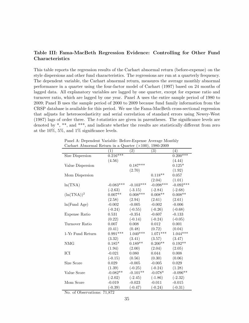
Table III: Fama-MacBeth Regression Evidence: Controlling for Other FundCharacteristics

This table reports the regression results of the Carhart abnormal return (before-expense) on thestyle dispersions and other fund characteristics. The regressions are run at a quarterly frequency.The dependent variable, the Carhart abnormal return, measures the average monthly abnormalperformance in a quarter using the four-factor model of Carhart (1997) based on 24 months oflagged data. All explanatory variables are lagged by one quarter, except for expense ratio andturnover ratio, which are lagged by one year. Panel A uses the entire sample period of 1980 to2009; Panel B uses the sample period of 2000 to 2009 because fund family information from theCRSP database is available for this period. We use the Fama-MacBeth cross-sectional regressionthat adjusts for heteroscedasticity and serial correlation of standard errors using Newey-West(1987) lags of order three. The t-statistics are given in parentheses. The significance levels aredenoted by *, **, and ***, and indicate whether the results are statistically different from zeroat the 10%, 5%, and 1% significance levels.

Panel A: Dependent Variable: Before-Expense Average MonthlyCarhart Abnormal Return in a Quarter (×100), 1980-2009

(1) (2) (3) (4)Size Dispersion 0.216*** 0.200***

(4.56) (4.44)Value Dispersion 0.187*** 0.125*

(2.70) (1.92)Mom Dispersion 0.118** 0.057

(2.04) (1.01)ln(TNA) -0.083*** -0.103*** -0.098*** -0.092***

(-2.63) (-3.15) (-2.84) (-2.68)(ln(TNA))2 0.007** 0.008*** 0.008** 0.008**

(2.58) (2.94) (2.61) (2.61)ln(Fund Age) -0.002 -0.005 -0.002 -0.006

(-0.24) (-0.55) (-0.26) (-0.68)Expense Ratio 0.531 -0.354 -0.607 -0.133

(0.22) (-0.14) (-0.24) (-0.05)Turnover Ratio 0.007 0.008 0.012 0.001

(0.41) (0.48) (0.72) (0.04)1-Yr Fund Return 0.991*** 1.040*** 1.071*** 1.044***

(3.32) (3.41) (3.57) (3.47)NMG 0.185* 0.189** 0.200** 0.192**

(1.94) (2.00) (2.04) (2.05)ICI -0.021 0.080 0.044 0.008

(-0.15) (0.56) (0.30) (0.06)Size Score 0.029 -0.005 -0.005 0.029

(1.39) (-0.25) (-0.24) (1.28)Value Score -0.082** -0.101** -0.078* -0.096**

(-2.02) (-2.45) (-1.86) (-2.32)Mom Score -0.019 -0.023 -0.011 -0.015

(-0.39) (-0.47) (-0.24) (-0.31)No. of Observations: 71,872

35

Table III (Continued)

Panel B: Dependent Variable: Before-Expense Average MonthlyCarhart Abnormal Return in a Quarter (×100), 2000-2009

(1) (2) (3) (4)Size Dispersion 0.141* 0.133** 0.150** 0.142**

(2.00) (2.02) (2.17) (2.20)

Top 10 Family (based on Family TNA) -0.004 -0.004(-0.18) (-0.14)

Top 10 Family (based on Family TNA)×Size Dispersion 0.093 0.093(1.28) (1.20)

Top 10 Family (based No. of Inv. Obj.) -0.001 -0.001(-0.04) (-0.03)

Top 10 Family (based on No. of Inv. Obj.)×Size Dispersion 0.043 0.039(0.68) (0.62)

Value Dispersion 0.089 0.088(0.77) (0.77)

Mom Dispersion 0.102 0.103(1.35) (1.38)

ln(TNA) 0.007 0.007 0.006 0.006(0.27) (0.28) (0.22) (0.25)

(ln(TNA))2 -0.001 -0.001 -0.000 -0.000(-0.29) (-0.36) (-0.18) (-0.27)

ln(Fund Age) 0.007 0.007 0.006 0.007(0.70) (0.71) (0.65) (0.67)

Expense Ratio 2.226 2.028 1.925 1.711(0.87) (0.81) (0.77) (0.70)

Turnover Ratio -0.012 -0.013 -0.011 -0.013(-0.87) (-1.06) (-0.84) (-1.04)

1-Yr Fund Return 0.668 0.675 0.673 0.681(1.16) (1.19) (1.16) (1.19)

NMG 0.131 0.127 0.136 0.133(1.48) (1.46) (1.52) (1.52)

ICI 0.212 0.247 0.225 0.262*(1.39) (1.65) (1.47) (1.74)

Size Score 0.048 0.044 0.050 0.046(1.36) (1.28) (1.41) (1.34)

Value Score -0.061 -0.066 -0.063 -0.068(-0.86) (-0.93) (-0.89) (-0.96)

Mom Score -0.078 -0.074 -0.079 -0.075(-0.71) (-0.67) (-0.71) (-0.67)

No. of Observations: 50,801

36

Table IV: Fama-MacBeth Regression Evidence: Controlling for IdiosyncraticRisk and Survivorship Using the Appraisal Ratio

This table reports the regression results of the appraisal ratio (before-expense) on the styledispersions and other fund characteristics for the period of 1980 to 2009. The regressions arerun at a quarterly frequency. The dependent variable, the appraisal ratio, measures the averagemonthly abnormal performance in a quarter scaled by idiosyncratic volatility estimated using thefour-factor model of Carhart (1997) based on 24 months of lagged data. All explanatory variablesare lagged by one quarter, except for expense ratio and turnover ratio, which are lagged by oneyear. We use the Fama-MacBeth cross-sectional regression that adjusts for heteroscedasticity andserial correlation of standard errors using Newey-West (1987) lags of order three. The t-statisticsare given in parentheses. The significance levels are denoted by *, **, and ***, and indicatewhether the results are statistically different from zero at the 10%, 5%, and 1% significancelevels.

Dependent Variable: Before-Expense Average MonthlyAppraisal Ratio in a Quarter

(1) (2) (3) (4)Size Dispersion 0.171*** 0.160***

(4.47) (4.39)Value Dispersion 0.152*** 0.111**

(2.85) (2.21)Mom Dispersion 0.050 0.001

(1.15) (0.01)ln(TNA) -0.025 -0.043** -0.038* -0.033

(-1.18) (-2.11) (-1.71) (-1.48)(ln(TNA))2 0.002 0.003 0.003 0.003

(1.04) (1.65) (1.29) (1.33)ln(Fund Age) 0.004 0.002 0.003 0.001

(0.47) (0.25) (0.42) (0.11)Expense Ratio 2.183 1.364 1.130 1.479

(1.10) (0.65) (0.53) (0.74)Turnover Ratio -0.007 -0.006 -0.002 -0.011

(-0.58) (-0.51) (-0.22) (-1.08)1-Yr Fund Return 0.748*** 0.769*** 0.805*** 0.778***

(3.67) (3.67) (3.88) (3.75)NMG 0.115** 0.119** 0.125** 0.121**

(2.03) (2.06) (2.19) (2.13)ICI -0.097 -0.012 -0.054 -0.086

(-1.34) (-0.17) (-0.74) (-1.26)Size Score 0.026* -0.002 -0.002 0.025

(1.79) (-0.13) (-0.16) (1.64)Value Score -0.063** -0.077** -0.061* -0.077**

(-1.99) (-2.24) (-1.85) (-2.24)Mom Score -0.011 -0.015 -0.011 -0.016

(-0.37) (-0.46) (-0.34) (-0.49)No. of Observations: 71,872

37

Table V: Fama-MacBeth Regression Evidence: Decomposing Size Dispersioninto “Deviation-Only” and “Distance-Only” Measures

This table reports the regression results of the Carhart abnormal return (before-expense) onsize dispersion and its deviation-only and distance-only components for the period of 1990 to2006, due to availability of the Active Share (proxy of the distance-only measure) data. Theregressions are run at a quarterly frequency. The dependent variable, the Carhart abnormalreturn, measures the average monthly abnormal performance in a quarter using the four-factormodel of Carhart (1997) based on 24 months of lagged data. All explanatory variables are laggedby one quarter, except for expense ratio and turnover ratio, which are lagged by one year. Weuse the Fama-MacBeth cross-sectional regression that adjusts for heteroscedasticity and serialcorrelation of standard errors using Newey-West (1987) lags of order three. The t-statistics aregiven in parentheses. The significance levels are denoted by *, **, and ***, and indicate whetherthe results are statistically different from zero at the 10%, 5%, and 1% significance levels.

38

Table V (Continued)

Dependent Variable: Before-Expense Average MonthlyCarhart Abnormal Return in a Quarter (×100), 1990-2006

(1) (2) (3) (4)Size Dispersion 0.186***

(2.88)Distance-Only 0.248*** 0.290***

(3.39) (3.41)Deviation-Only (Active Share) 0.214 0.242

(1.32) (1.41)Value Dispersion 0.039 0.105 0.110 0.098

(0.44) (1.11) (1.20) (1.10)Mom Dispersion 0.121* 0.101 0.097 0.093

(1.68) (1.27) (1.21) (1.19)ln(TNA) -0.043 -0.049 -0.050 -0.047

(-1.62) (-1.62) (-1.51) (-1.42)(ln(TNA))2 0.004 0.003 0.003 0.003

(1.53) (1.22) (1.25) (1.17)ln(Fund Age) -0.010 0.002 -0.001 0.002

(-1.20) (0.17) (-0.13) (0.22)Expense Ratio 0.498 -1.456 -1.799 -1.793

(0.30) (-0.64) (-0.85) (-0.87)Turnover Ratio -0.005 -0.013 -0.012 -0.012

(-0.30) (-0.73) (-0.66) (-0.65)1-Yr Fund Return 1.195*** 1.226*** 1.231*** 1.218***

(4.06) (4.50) (4.53) (4.44)NMG -0.014 0.050 0.040 0.042

(-0.16) (0.55) (0.47) (0.50)ICI 0.176 0.136 0.014 0.003

(1.36) (0.47) (0.05) (0.01)Size Score -0.007 -0.030 -0.017 -0.009

(-0.30) (-1.42) (-0.65) (-0.36)Value Score -0.027 -0.023 -0.023 -0.022

(-0.60) (-0.54) (-0.57) (-0.53)Mom Score -0.094* -0.104 -0.094 -0.094

(-1.75) (-1.46) (-1.37) (-1.41)No. of Observations: 33,759

39

Table VI: Holding-Based Performance Measures of Portfolios Based on SizeDispersion

This table reports the two holding-based performance measures proposed by DGTW (1997),the “Characteristic Selectivity” measure CS and the “Characteristic Timing” measure CT, fordecile portfolios based on size dispersion for the period of 1980 to 2009. We form 10 portfoliosat the beginning of each quarter based on the lagged size dispersion. The equally-weighteddecile CS and CT measures are expressed at a monthly frequency. The t-statistics are givenin parentheses. The table also reports the differences in the performance measures, along withtheir t-statistics, between the top and the bottom deciles and between the top and the bottomhalves. The significance levels are denoted by *, **, and ***, and indicate whether the resultsare statistically different from zero at the 10%, 5%, and 1% significance levels.

Monthly Holding-Based Performance Measuresof Portfolios Based on Size Dispersion (×100)

CS CT(1) (2)

1 (Low Size Disp.) 0.078 -0.044(0.29) (-1.38)

2 0.081 -0.038(0.30) (-1.46)

3 0.087 -0.045(0.31) (-1.55)

4 0.081 -0.007(0.28) (-0.29)

5 0.088 0.012(0.29) (0.56)

6 0.127 -0.012(0.41) (-0.54)

7 0.195 -0.007(0.60) (-0.30)

8 0.192 -0.016(0.60) (-0.58)

9 0.252 -0.030(0.78) (-1.30)

10 (High Size Disp.) 0.349 0.008(1.10) (0.32)

Decile 10-Decile 1 0.271** 0.051(2.23) (1.50)

2nd half-1st half 0.140* 0.013(1.68) (0.69)

40

Table VII: “Characteristic Selectivity” (CS) Measures of Portfolios Based onSize Dispersion: A Diagnostic Analysis

This table reports the “Characteristic Selectivity” measure CS for the “near” and “far” portfoliosin each decile based on size dispersion for the period of 1980 to 2009. We form 10 portfolios at thebeginning of each quarter based on the lagged size dispersion. For each fund in a decile, we divideits stockholdings into “near” and “far” portfolios based on the distance from the fund’s core sizestyle, and compute their CS measures. The equally-weighted decile CS measures are expressedat a monthly frequency. The t-statistics are given in parentheses. The table also reports thedifferences in the CS measures, along with their t-statistics, between the top and the bottomdeciles, between the top and the bottom halves, and between “near” and “far” portfolios. Thesignificance levels are denoted by *, **, and ***, and indicate whether the results are statisticallydifferent from zero at the 10%, 5%, and 1% significance levels.

Monthly “Characteristic Selectivity” (CS) Measures of Portfolios Based on Size Dispersion (×100)Portfolios according to Median Portfolios according to 75th percentileDistance of Decile Stockholdings Distance of Decile Stockholdings“Near” “Far” Diff. “Near” “Far” Diff.(1) (2) (3)=(2)-(1) (4) (5) (6)=(5)-(4)

1 (Low Size Disp.) 0.070 0.063 -0.007 0.087 0.061 -0.026(0.26) (0.22) (-0.08) (0.33) (0.20) (-0.21)

2 0.072 0.132 0.060 0.082 0.138 0.056(0.27) (0.44) (0.64) (0.30) (0.42) (0.43)

3 0.063 0.124 0.061 0.085 0.087 0.001(0.23) (0.39) (0.59) (0.31) (0.25) (0.01)

4 0.102 0.093 -0.009 0.095 0.073 -0.022(0.36) (0.30) (-0.13) (0.34) (0.21) (-0.19)

5 0.050 0.171 0.121* 0.054 0.257 0.203*(0.17) (0.53) (1.71) (0.18) (0.76) (1.93)

6 0.096 0.158 0.062 0.120 0.237 0.117(0.31) (0.48) (0.99) (0.39) (0.68) (1.06)

7 0.163 0.296 0.133* 0.164 0.332 0.167*(0.50) (0.88) (1.93) (0.52) (0.92) (1.76)

8 0.181 0.205 0.024 0.171 0.246 0.075(0.56) (0.62) (0.36) (0.54) (0.68) (0.68)

9 0.228 0.286 0.058 0.245 0.373 0.128(0.70) (0.86) (0.76) (0.77) (1.05) (1.25)

10 (High Size Disp.) 0.316 0.371 0.055 0.322 0.477 0.155(0.98) (1.11) (0.67) (1.02) (1.33) (1.35)

Decile 10-Decile 1 0.246* 0.308** 0.234* 0.416**(1.87) (2.23) (1.89) (2.40)

2nd half-1st half 0.129 0.144* 0.124 0.203**(1.42) (1.72) (1.45) (2.01)

41

Appendix A

Table A.I: After-Expense Returns of Portfolios Based on Style Dispersions

This table reports the five risk- and style-adjusted returns (after-expense) of decile portfoliosbased on the size, value, and momentum dispersions, respectively, for the period of 1980 to 2009.We form 10 portfolios at the beginning of each quarter based on each lagged style dispersion.The equally-weighted decile returns are expressed at a monthly frequency. We use excess returnover the market, and abnormal returns of CAPM, the Fama-French three-factor model, theCarhart four-factor model, and the Pastor-Stambaugh five-factor model. The t-statistics aregiven in parentheses. The table also reports the differences in these returns, along with theirt-statistics, between the top and the bottom deciles and between the top and the bottom halves.The significance levels are denoted by *, **, and ***, and indicate whether the results arestatistically different from zero at the 10%, 5%, and 1% significance levels.

Panel A: After-Expense Monthly Returns of Portfolios Based on Size Dispersion (×100)Excess Return CAPM Fama-French Carhart Pastor-Stambaugh(1) (2) (3) (4) (5)

1 (Low Size Disp.) -0.153*** -0.109*** -0.066** -0.046 -0.043(-3.71) (-2.93) (-2.23) (-1.55) (-1.40)

2 -0.108*** -0.086** -0.053 -0.032 -0.023(-2.91) (-2.36) (-1.59) (-0.95) (-0.66)

3 -0.122*** -0.107*** -0.093*** -0.096*** -0.086***(-3.74) (-3.30) (-2.90) (-2.94) (-2.60)

4 -0.070 -0.053 -0.060 -0.058 -0.033(-1.62) (-1.24) (-1.39) (-1.31) (-0.74)

5 -0.043 -0.053 -0.071 -0.078* -0.064(-0.87) (-1.07) (-1.57) (-1.68) (-1.37)

6 0.016 -0.008 -0.027 -0.056 -0.057(0.25) (-0.12) (-0.50) (-1.05) (-1.04)

7 0.066 0.024 0.003 -0.030 -0.021(0.82) (0.31) (0.05) (-0.55) (-0.38)

8 0.137 0.083 0.065 0.013 0.027(1.55) (0.96) (1.16) (0.23) (0.47)

9 0.131 0.080 0.043 0.001 0.015(1.44) (0.90) (0.83) (0.02) (0.28)

10 (High Size Disp.) 0.209** 0.162* 0.134*** 0.095* 0.114**(2.39) (1.89) (2.61) (1.85) (2.19)

Decile 10-Decile 1 0.361*** 0.272** 0.200*** 0.142** 0.156**(3.15) (2.48) (3.26) (2.33) (2.54)

2nd half-1st half 0.211*** 0.150** 0.112*** 0.067* 0.065*(2.69) (2.00) (2.94) (1.79) (1.72)

42

Table A.I (Continued)

Panel B: After-Expense Monthly Returns of Portfolios Based on Value Dispersion (×100)Excess Return CAPM Fama-French Carhart Pastor-Stambaugh(1) (2) (3) (4) (5)

1 (Low Value Disp.) -0.068 -0.157 -0.019 -0.027 0.001(-0.64) (-1.57) (-0.28) (-0.40) (0.01)

2 -0.076 -0.102* -0.051 -0.067 -0.050(-1.33) (-1.80) (-1.26) (-1.62) (-1.21)

3 -0.026 -0.039 -0.024 -0.043 -0.024(-0.53) (-0.78) (-0.56) (-1.02) (-0.56)

4 0.011 0.021 0.002 -0.004 0.007(0.25) (0.49) (0.05) (-0.11) (0.18)

5 -0.008 0.006 -0.036 -0.049 -0.036(-0.18) (0.14) (-0.97) (-1.29) (-0.95)

6 0.019 0.028 -0.007 -0.025 -0.014(0.44) (0.65) (-0.17) (-0.62) (-0.33)

7 0.033 0.038 -0.003 -0.016 -0.013(0.69) (0.79) (-0.06) (-0.37) (-0.28)

8 -0.014 -0.015 -0.055 -0.064 -0.058(-0.27) (-0.28) (-1.20) (-1.36) (-1.22)

9 0.071 0.059 0.014 -0.011 -0.003(1.30) (1.07) (0.30) (-0.24) (-0.06)

10 (High Value Disp.) 0.114* 0.087 0.046 0.012 0.016(1.75) (1.34) (0.84) (0.21) (0.28)

Decile 10-Decile 1 0.182* 0.244** 0.065 0.038 0.015(1.83) (2.52) (0.82) (0.47) (0.18)

2nd half-1st half 0.078** 0.094** 0.025 0.017 0.006(1.98) (2.39) (0.73) (0.49) (0.17)

43

Table A.I (Continued)

Panel C: After-Expense Monthly Returns of Portfolios Based on Momentum Dispersion (×100)Excess Return CAPM Fama-French Carhart Pastor-Stambaugh(1) (2) (3) (4) (5)

1 (Low Mom Disp.) -0.028 -0.105 0.050 -0.050 -0.051(-0.21) (-0.81) (0.54) (-0.54) (-0.55)

2 -0.027 -0.067 0.008 -0.060 -0.052(-0.35) (-0.89) (0.14) (-1.13) (-0.96)

3 -0.006 -0.012 0.001 -0.052 -0.046(-0.11) (-0.23) (0.03) (-1.20) (-1.06)

4 -0.000 0.010 -0.017 -0.039 -0.033(-0.00) (0.26) (-0.46) (-1.07) (-0.89)

5 -0.034 -0.018 -0.054 -0.061 -0.049(-0.83) (-0.45) (-1.44) (-1.59) (-1.26)

6 -0.016 -0.002 -0.045 -0.041 -0.025(-0.34) (-0.05) (-0.99) (-0.88) (-0.54)

7 0.050 0.060 0.002 0.015 0.030(0.93) (1.11) (0.05) (0.29) (0.56)

8 0.047 0.044 -0.009 -0.000 0.018(0.82) (0.76) (-0.16) (-0.00) (0.32)

9 0.002 -0.005 -0.061 -0.035 -0.020(0.04) (-0.08) (-1.08) (-0.61) (-0.34)

10 (High Mom Disp.) 0.069 0.022 -0.008 0.028 0.054(0.91) (0.30) (-0.12) (0.42) (0.81)

Decile 10-Decile 1 0.097 0.127 -0.058 0.077 0.105(0.69) (0.90) (-0.46) (0.62) (0.83)

2nd half-1st half 0.049 0.062 -0.021 0.046 0.057(0.77) (0.96) (-0.37) (0.80) (1.00)

44

Table A.II: Panel Regression Evidence: Controlling for Other Fund Charac-teristics

This table reports the regression results of the Carhart abnormal return (before-expense) on thestyle dispersions and other fund characteristics for the period of 1980 to 2009. The regressions arerun at a quarterly frequency. The dependent variable, the Carhart abnormal return, measuresthe average monthly abnormal performance in a quarter using the four-factor model of Carhart(1997) based on 24 months of lagged data. All explanatory variables are lagged by one quarter,except for expense ratio and turnover ratio, which are lagged by one year. We use the panelregression that includes the time fixed effects. Standard errors are adjusted for heteroscedasticityand clustered at the time level. The t-statistics are given in parentheses. The significance levelsare denoted by *, **, and ***, and indicate whether the results are statistically different fromzero at the 10%, 5%, and 1% significance levels.

Dependent Variable: Before-Expense Average MonthlyCarhart Abnormal Return in a Quarter (×100), 1980-2009

(1) (2) (3) (4)Size Dispersion 0.211*** 0.174***

(3.07) (2.75)Value Dispersion 0.204* 0.114

(1.87) (1.20)Mom Dispersion 0.307** 0.257*

(2.07) (1.80)ln(TNA) -0.017 -0.022 -0.022 -0.021

(-0.70) (-0.90) (-0.90) (-0.86)(ln(TNA))2 0.001 0.001 0.001 0.001

(0.43) (0.52) (0.47) (0.50)ln(Fund Age) 0.001 0.003 0.004 0.000

(0.10) (0.25) (0.35) (0.03)Expense Ratio 0.217 0.892 0.856 0.108

(0.12) (0.45) (0.43) (0.06)Turnover Ratio -0.002 -0.000 -0.002 -0.007

(-0.13) (-0.02) (-0.12) (-0.52)1-Yr Fund Return 0.565 0.587 0.622* 0.590

(1.46) (1.53) (1.67) (1.56)NMG -0.110 -0.103 -0.107 -0.107

(-0.67) (-0.63) (-0.66) (-0.65)ICI 0.235** 0.338*** 0.374*** 0.302***

(2.15) (2.94) (3.20) (2.65)Size Score 0.020 -0.015 -0.009 0.019

(0.86) (-0.71) (-0.44) (0.82)Value Score -0.069 -0.087 -0.057 -0.081

(-1.06) (-1.39) (-0.87) (-1.31)Mom Score -0.152* -0.157* -0.120 -0.130

(-1.88) (-1.93) (-1.48) (-1.60)No. of Observations: 71,872

45