Embed Size (px)
Citation preview
1
The Mutual Fund Fee Puzzle
Michael Cooper, Michael Halling and Wenhao Yang *
August 2015
Keywords: mutual funds, fund fees, fund expenses, price dispersion, price persistence.
JEL Classifications: G10, G11, G23.
* Cooper and Yang are with the David Eccles School of Business, University of Utah. Halling is with the Stockholm School of
Economics and the Swedish House of Finance. We thank Jack Bogle, Darwin Choi, James Choi (WFA discussant), Susan
Christoffersen, Magnus Dahlquist, Monika Gehde-Trapp (discussant), Amit Goyal, Joseph Halford, Rachel Hayes, Keith Jacob,
Stephan Jank (discussant), Dong Lou (discussant), Veronika K. Pool (discussant), Jonathan Reuter, David Robinson, Norman
Schuerhoff, Mark Seasholes, Paolo Sodini, Laura Starks, Paul Tetlock, and Charles Trzcinka. We also thank participants of the
CEPR ESSFM meetings (2011, asset pricing week), the Northern Finance Association Meetings (2011), the 2012 WFA
meetings, the Austrian Working Group on Banking and Finance (2013), the 12th FBI Symposium in Karlsruhe (2014), and
seminar participants at Arizona State, HEC Lausanne, the Institute of Advanced Studies in Vienna, KAIST, Nanyang Tech
University, the Shanghai Advanced Institute of Finance, the University of Arizona, the University of Colorado, the University
of Montana, the University of California, San Diego, and VU University Amsterdam for their comments. An earlier version of
this paper was titled “Violations of the Law of One Fee in the Mutual Fund Industry.” Particular thanks go to Michael Lemmon
for his contributions to this earlier version of the paper.

2
The Mutual Fund Fee Puzzle
Abstract
We find economically large fee dispersion in the mutual fund industry, even after controlling for a
comprehensive set of fund characteristics such as performance, activeness or risk exposures. This dispersion is not
driven by small funds, as it is also substantial among the very largest funds (top quintile). It is also not driven by
the early years of the sample; rather in contrast, dispersion measures show a tendency to increase until the late-
90ties, to then stay at elevated levels until the recent financial crisis, and to only decrease slightly in most recent
years. Further tests reveal that competition and frictions help explain expected fees but do not substantially lower
fee dispersion. Interestingly, shocks to US household participation in the mutual fund industry significantly predict
future increases in dispersion (and, to a lesser extent, in average fees).
3
1. Introduction
A large literature exists that attempts to explain why similar products sell for different prices. For example,
Lach (2002) documents considerable price dispersion for similar refrigerators, chicken, coffee, and flour.1 He
concludes that because stores change their pricing on a regular basis, consumers cannot learn which stores are the
low cost sellers, and as a consequence, price dispersion persists.
In the mutual fund markets, Elton, Gruber, and Busse (2004) document price dispersion of more than 2% per
year for essentially identical S&P500 index funds. They conclude that a combination of the inability to arbitrage
(i.e., one cannot short sell open-ended mutual funds) and uninformed investors is sufficient to have the law of one
price fail in the S&P500 index fund market. Other research, focusing on sub-categories of funds, provides evidence
of differential prices being charged for funds with similar characteristics.2
In contrast, other papers suggest that the mutual fund markets are more or less competitively priced. For
example, Khorana, Servaes, and Tufano (2009) examine mutual fund fees in 18 countries and find that most of the
cross-sectional dispersion in fees can be explained by economic variables, such as investment objective, sponsor,
national characteristics, and levels of investor protection.3 More recently, Wahal and Wang (2011) provide evidence
that incumbents with high overlap in their portfolio holdings with entrants subsequently engage in price competition
by reducing their management fees. In addition, they also find evidence that incumbents with higher portfolio
overlap with entrants have lower future fund inflows. They conclude that the mutual fund market has “evolved into
one that displays the hallmark features of a competitive market.” Overall, while the existing literature provides
1 See also Bakos (2001), Brown and Goolsbee (2002), Brynjolfsson and Smith (2000), Nakamura (1999), Pratt, et al. (1979),
Scholten and Smith (2002), and Sorensen (2000). 2 See also Elton, Gruber, and Rentzler (1989) who find that public commodity funds exist that underperform the risk free rate,
Christoffersen and Musto (2002) who find a wide dispersion in expenses across similar money market funds, and Hortacsu and
Syverson (2004) who document fee dispersion within similar equity fund categories and within S&P500 index funds. There
are also several papers that develop theoretical models of the mutual fund industry, including endogenous fee setting. Nanda,
Narayanan and Warther (2000), for example, concentrate on the structure of mutual funds, i.e., on the combination of loads
and fees; Das and Sundaram (2002) compare fulcrum fees to incentive fees. Pastor and Stambaugh (2010) use their model to
study the aggregate size of the active management mutual fund market. 3 See also Khorana and Servaes (2009) who examine determinants of mutual fund family market share. They document that
fund families that charge lower style-adjusted expenses relative to other families and families whose expense ratios decline as
the fund family size grows have higher market share. They also find that families whose expenses are above the mean increase
their market share when they lower their expenses.
4
evidence of price dispersion in specific areas of the mutual fund market, there is little existing evidence on how
widespread the phenomenon is or on how it has changed over time given the dramatic growth in the mutual fund
market.
In this paper, we study the price dispersion among mutual funds and, specifically, investigate if similar funds,
as measured by important fund characteristics, have roughly similar expenses. To do this, we examine the residuals
from yearly, cross-sectional regressions of total annual expenses (i.e., annual operating expenses, including
management fees and 12b-1 fees) on lagged fund characteristics, such as risk and performance characteristics, extent
of active management, service levels, and fund size or age. On average, these regressions explain only about 28%
of the dispersion in expenses, leaving a sizable unexplained dispersion in expenses. Specifically, we find that the
average spread in residual expenses (between the 1st and 99th percentile) across all funds over the sample is 2.47%.
More interestingly, the dispersion in residual expenses has not decreased over time. In fact, the opposite is the
case, as dispersion increased until the late-90ties, then stayed at high levels for some years and only showed a slight
decrease in most recent years. In contrast, average fee levels – after increasing substantially until 2003 or so – did
experience a noticeable decrease during the last 10 to 15 years. Importantly, our results hold for both the largest
total net asset (TNA) funds as well as the smaller TNA funds; the average spread in residual expenses is 3.99% for
the smallest quintile of TNA funds and is 1.77% for the largest quintile of funds. Our results are robust to multiple
variations in the models used to estimate residual expenses, aggregation of share classes, the use of before-expense
performance measures in estimating residual expenses, and the use of holdings data to identify similar funds.
We examine the implications of our findings for investors. Based on residual expenses, an investor purchasing
the lowest expense funds would have earned compounded abnormal returns 84% higher than an investor purchasing
the most expensive funds. If we do the same exercise using reported expenses (i.e., a fund’s stated total annual
expenses), the low fee investor would have been 162% ahead of the high fee investor. As a basis for comparison,
the compounded differences in reported expenses (residual expenses) over the same period were 179% (147%).
Thus, while the difference in abnormal returns between high expense and low expense funds is less than the

5
cumulative difference in expenses, investors bear significant costs from investing in high expense mutual funds that
are not recouped through higher performance of these funds.
One interpretation of our results on fee dispersion is lack of competition among mutual funds, consistent with
Haslem, Baker and Smith (2006), Gil-Bazo and Ruiz-Verdu (2009), and Barras, Scaillet and Wermers (2010). In
contrast, however, Wahal and Wang (2011) conclude that the mutual fund industry behaves like a competitive
industry. To shed some more light on these differing results, we follow Wahal and Wang (2011) and create a fund-
level competition measure based on holdings information. Consistent with their results and economic theory, we
find some evidence that funds facing competition charge lower fees; however, controlling for competition in the
fee regressions does not result in a substantial reduction of residual fee dispersion.
Finally, we investigate mechanisms that could potentially inhibit competition and boost dispersion. One such
mechanism relies on the existence of frictions such as search costs or barriers to exit from funds. We define
empirical proxies for these frictions and find strong and statistically significant evidence that they matter for
expected fees – funds that seem to engage in randomization of fee changes and funds that make it costly for investors
to exit are able to charge higher fees. Interestingly and surprisingly, however, controlling for these factors in the
fee regressions does not reduce the spreads in residual fees.
Another mechanism that prevents competition and should increase fee dispersion is based on the existence of
investor clienteles. Here we follow Christoffersen and Musto (2002) and Gil-Bazo and Ruiz-Verdu (2008) who
argue that performance-sensitive investors withdraw assets from poorly performing funds leaving only
performance-insensitive investors as holders of the funds’ shares; in response, poorly performing funds tend to
increase their fees. We find no support for this mechanism in our sample. Alternatively, we investigate whether
the time-series dynamics of fee dispersion and average levels of fees are related to the participation of retail investors
in the mutual fund industry. We find strong evidence that this is the case: positive shocks to the participation of
retail investors resulted in subsequent increases in fee dispersion and average levels of fees.
The above results seem puzzling to us. While average fee levels have decreased in recent years, consistent
with competition working well, levels of fee dispersion are still at economically large levels suggesting that

6
competition does not work that well. Similarly, while our proxies for frictions help explain fees, they have only a
negligible impact on fee dispersion. Maybe our proxies are not capturing the corresponding frictions well or we
are missing important frictions in our analysis.
Alternatively, if one takes it as a given that the mutual fund markets are in a competitive equilibrium, then our
finding of a large dispersion in prices for similar funds still represents a puzzle: what mutual fund product
characteristics, missing from our analysis, can explain such large spreads in fees? Stated differently, what omitted
product characteristics can be so important to investors that they are willing to lose 84% or more of the future value
of their portfolio?
We see the broader contribution of this paper as threefold. First, we show that the S&P 500 index fund price
dispersion effects documented in Elton, Gruber, and Busse (2004) and Hortacsu and Syverson (2004) extend to the
entire US equity fund industry. We find that the spread in prices among similar funds is pervasive across investment
styles, institutional and non-institutional funds, and for small and large TNA funds. In addition, despite enormous
industry growth, the effect has not diminished much over time. Second, the heterogeneity of funds in our sample,
relative to prior work in this area using index funds, allows us to test a rich set of hypotheses to explain fee
dispersion, resulting in a deeper understanding of how funds set fees. Finally, we show important investor welfare
effects that are industry wide and not just applicable to small subsets of funds.
The remainder of the paper is organized as follows. In Section 2 we describe the data used in our analysis and
describe the characteristics of high and low expense funds. In Section 3 we present results that document price
dispersion in the residual expense distribution of funds and perform tests to quantify the economic effects of expense
dispersion for fund investors. In Section 4, we test various hypotheses to explain the residual expense dispersion of
funds. Section 5 concludes.

7
2. Data
2.1 Sample Construction
The sample selection follows Pastor and Stambaugh (2002). Accordingly, we select only domestic equity
funds and exclude all funds not investing primarily in equities such as money market or bond funds. In addition,
we exclude international funds, global funds, balanced funds, flexible funds, and funds of funds. The ICDI
classification codes that were used by Pastor and Stambaugh (2002) are, however, no longer available. Thus, we
follow Bessler et al. (2008) who use a combination of Lipper codes, Wiesenberger codes and Strategic Insight codes
to identify domestic equity funds. Table A in the Data Appendix lists the specific codes that we use to identify the
funds in our sample.
In short, the above screens result in our sample focusing on active and passive US domestic equity funds. Our
sample includes approximately 38% of all funds covered in the CRSP Mutual Fund Database (our sample consists
of a total of 20,926 funds while the CRSP Mutual Fund Database universe has approximately 55,109 funds). As
measured by total net assets, our sample covers approximately 42.5% of the cumulative net assets represented in
the database. The sample period spans 1966 to 2014 and the data frequency is yearly, as we focus on fund expenses.
2.2 Descriptive Statistics
Table 1 Panel A reports summary statistics of our fund sample. Details of the variable construction can be
found in Table B in the Data Appendix. Throughout the paper we distinguish between a pre-1999 (up to and
including 1998) and a post-1999 (including 1999) sample because several important variables such as fund family
information (i.e., information on management companies) and flags for institutional funds only became available
in the CRSP Mutual Fund Database in 1999.
The descriptive statistics show the dramatic increase in mutual funds over the past 30 years. In the pre-1999
sample the mean number of funds per year is 1051, while it increases to 7931 in the post-1999 sample. Note that
the mean fund size (TNA) also increases from 361 Million USD pre-1999 to 530 Million USD post-1999. Thus,
the mutual fund industry has experienced a considerable increase in assets under management.
8
Intuitively, given more funds and thus presumably increased competition, we would have expected to find that
the rapid expansion of the mutual fund industry was also accompanied by a decrease in average expense ratios –
but this is not the case.4 Average annual expense ratios (expense ratio) increased from 121 basis points (bps) to
138 bps. It is also interesting to observe that yearly changes of expense ratios (Δ(expense ratio)) are on average
close to zero. This is mostly driven by the fact that, on average, a similar fraction of funds increases and decreases
their fees, namely 32% and 33% of all funds in a given year, respectively. Thus, if we remove the signs of the fee
changes and calculate the time-series average of cross-sectional mean absolute fee changes, we find that it
corresponds to 22 basis points; a relatively large number in economic terms.
The average performance of our sample funds, as measured by annual four-factor alphas (Carhart (1997)), is
negative (-1.4% in pre-1999 and -1.2% in post-1999), consistent with Carhart (1997) and others who show that
funds do not earn positive abnormal returns net of expenses. The average fund, over both time periods, has a market
beta (beta_mkt) that is slightly less than 1, a small, negative exposure to HML (beta_hml), and small positive
exposures to SMB (beta_smb) and UMD (beta_umd). After 1999, funds load more on the market, and less on SMB,
HML, and UMD, consistent with an aggregate strategy shift to market indexing. The four-factor model works very
well on average in explaining fund returns, yielding R2 of 78% and 87%, in the pre and post-1999 periods,
respectively.
Panel B (pre-1999 sample) and Panel C (post-1999 sample) of Table 1 report summary statistics by expense
ratio deciles. Each year we split all funds into deciles by their expense ratios and then report contemporaneous
means and standard deviations of fund characteristics.
Average expense ratios (expense ratio) of decile 10 exceed those of decile 1 by roughly 230 bps, in both the
pre-1999 and post-1999 periods. In the pre-1999 sample, average expense ratio changes are most negative (-14
bps) in decile 1 and most positive (42 bps) in decile 10. These mean changes become smaller in the post-1999
4 The averages reported in Table 1 are equal-weighted. If we value weight the expenses, we find a slight decrease from pre to
post-1999. In this case, the corresponding values are 87 bps for pre-1999 expenses and 78 for post-1999 expenses. Figure 6
shows the complete time-series dynamics for value-weighted average fees.
9
sample: funds in the bottom expense ratio decile decrease their expenses on average by 1 bps in the same year,
while funds in the top decile increase their expenses on average by 6 bps in the same year.
All of the fund performance variables decrease by expense ratio deciles. The spread in yearly four-factor
Carhart alphas, for example, equals 2.0% pre-1999 and 1.8% post-1999, which is comparable to the spread in
expense ratios, especially post-1999. Thus, these simple descriptive statistics suggest that funds with higher
expense ratios on average underperform their cheaper competitors by approximately their expense ratios.
We also find that average fund size (TNA) in decile 1 is much larger than average size in decile 10, suggesting
that economies of scale play a role for expense ratios. The average size in decile 1 is approximately 1.9 Billion
USD larger in both the pre-1999 and post-1999 periods than the average size fund in expense ratio decile 10. We
also find a greater concentration of fund families (Family dummies) in the lower expense deciles, although there are
a non-trivial number of funds that belong to large fund families that reside in the higher expense deciles. For
example, 57% of the funds in expense decile one are funds that belong to a fund family with more than 100 funds
and 46% in expense decile ten are funds that belong to a fund family with more than 100 funds.5 Moreover, we
also find a greater concentration of institutional funds (Institutional dummy) and ETFs (ETF dummy) in the lower
expense deciles.
Finally, Panel D of Table 1 shows pooled correlations between fund characteristics. These correlations are
consistent with our previous interpretations of patterns between expense ratio deciles and other fund characteristics.
In general, none of these correlations seem to be high enough to cause worries about multi-collinearity problems in
the subsequent multivariate analysis.
Of course, the most important limitation of this univariate analysis from Table 1 is that it ignores that expense
ratios may reflect different fund strategies and characteristics. This is something that we will explore in more detail
in later sections of the paper. These simple summary statistics, however, already suggest that to some extent,
expense ratios can be explained by economic determinants. For example, funds’ risk characteristics seem to be
5 In later cross-sectional tests we find that large families charge greater expenses.

10
correlated with expense ratios: more expensive funds tend to exhibit higher absolute loadings on standard risk
factors (i.e., on MKT, SMB, and UMD). Similarly, the average R2 of the four-factor model decreases as we move
from decile 1 to decile 10, suggesting that the managers of the higher expense funds may be following “unique”
strategies, likely in an attempt to outperform. However, these managers also trade much more (i.e., the turnover is
much higher for the high expense funds relative to the low expense funds), which may contribute to their low return
performance. Overall, these patterns between risk characteristics and expense ratios are intuitive and suggest that
expensive funds do follow, at least to some extent, more active strategies, load more aggressively on individual risk
factors, and implement strategies that go beyond the standard risk factors.
3. The Pricing of Mutual Funds
3.1 Residual Expense Estimation and the Pricing of Individual Fund Characteristics
Our goal is to compare prices (total expense ratios including management expenses and 12b-1 fees) across
funds. Of course, not all funds are the same and differences in fund characteristics might justify price differences.
Thus, we follow Lach (2002) and Sorensen (2000) to control for fund heterogeneity. As controls we use the standard
fund characteristics that have been shown to be important in determining fund expenses (e.g., see Gil-Bazo and
Ruiz-Verdu (2009) and Wahal and Wang (2011)).
We regress fund expenses on lagged fund characteristics including performance and risk characteristics. As
our set of explanatory variables changes over time (e.g., fund family information is only available after 1998), we
estimate a cross-sectional regression each year. Another advantage of this specification is that it allows for changing
relationships (i.e., time-varying coefficients) between fund characteristics and expenses. The residuals of these
regressions can be interpreted as deviations of fund expenses from expected expenses given the set of characteristics
used in the regression. Thus, using the residuals, we can compare prices across “identical” funds, under the
assumption that we have controlled for the correct fund characteristics.6
6 We don’t claim to have the absolutely correct expense models. We are careful to include fund characteristics that should
matter to the average investor. Many of these characteristics are related to fund performance – items that should be the first
order determinants of fund expenses. Mutual funds are, after all, investment portfolios and (most likely) not solely consumption
11
In Table 2 we present the details of the yearly cross-sectional regressions used to estimate the residuals. The
reported coefficients are time series averages of cross-sectional regression coefficients obtained from the annual
cross-sectional regressions. We estimate these models separately for the full sample and for the largest and smallest
quintile of annually-ranked TNA funds. We also standardize the independent variables to have a mean of zero and
a standard deviation of one. The standardized coefficients, thus, allow us to discuss a fund fee price estimate for a
one standard deviation change in each independent variable, and also allow us to rank the fund characteristics in
terms of economic importance.
For the full sample in the pre-1999 period, the models explain approximately 24% of the variation in expenses;
in the post-1999 period, the model explains 28%. The signs of the coefficients are mostly consistent with the
literature: e.g., across the two periods we observe that better performing funds (Annual return), less volatile funds
(sdmret), larger funds (TNA), younger funds (fund age), lower turnover funds (turnover), institutional funds
(Institutional dummy), ETFs (ETF dummy), and funds with higher R2 from the Carhart four-factor model have lower
expenses. Across the pre- and post-1999 periods, we essentially see the same relationships, with the exception of
some sign switching of the coefficients from the four-factor model.
In terms of economic importance or “pricing” of individual fund characteristics, we observe substantial
variation across variables. In the following, we discuss the fund characteristics from most to least expensive
according to the full sample results in the post-1999 period. Looking at the results for the full sample of funds, in
the post-1999 period, the coefficient on the institutional dummy is -53.62, suggesting that fund investors pay an
extra 54 bps for non-institutional funds on average. Also, investors pay 45 bps to be in non-ETF funds. Interestingly,
these prices of the institutional or the ETF feature vary significantly across our sub-samples of smallest and largest
funds. Specifically, it is roughly speaking twice as expensive to be non-institutional and non-ETF in the small than
in the large TNA fund universe.
products, and thus it seems reasonable to judge their performance using metrics from the asset pricing literature. However, we
also include service and other non-performance related characteristics in the expense models. In Section 3.6, we estimate fees
differences for similar funds using a model free approach that uses fund holdings information.
12
Investors pay 34 bps to purchase an extra unit of fund standard deviation of return, which can probably be
viewed as the price of buying a more active and less diversified fund. Interestingly, the price of a unit of standard
deviation is essentially zero within the large TNA group, and is 69 bps for the small TNA group.7 This pattern,
however, is different in the pre-1999 sample where investors paid around 25 basis points for an extra unit of fund
standard deviation within the large and the small TNA sample.
The prices for the R-square variable, with the idea that lower R-square signals a more active fund, also features
an interesting pattern: 22 (10) bps more for a unit of lower R-square for the small TNA funds and only 6 (0) bps
more within the large TNA funds in the post-1999 (pre-1999) sample period. Across all fund groups, investors also
pay more for smaller TNA funds; 24 bps per unit of Ln(TNA) for the full sample, with little variation across fund
groups, at least in the post-1999 period. Investors pay more for style exposure, but only for value/growth exposure,
and not size, market, or momentum exposure. For example, the price of an extra unit of SMB beta is 20 bps for the
full sample, but only 1 to 2 bps for the HML and momentum beta (with slightly larger prices for SMB, market, and
momentum betas for the small TNA funds).
As far as the price that investors pay for fund performance are concerned, the results seem counter-intuitive
because of the negative coefficient on lagged returns in the fee regressions. The negative sign, however, is
consistent with Christoffersen and Musto (2002) and Gil-Bazo and Ruiz-Verdu (2008) who argue that as fund
returns go down, performance sensitive investors exit the fund, leaving a majority of performance insensitive
investors, for whom fund management then raises the fees (see Section 4.3 for a more detailed discussion of this
mechanism). Fund investors pay 14 bps for a unit standard deviation of lower annual returns, and are much more
willing to pay this for the small TNA funds (i.e., they pay 40 bps for a one-standard deviation worse performance
within the small fund group). Importantly, past fund performance does not seem to be of first order importance for
fund fees. At least, in terms of the absolute magnitude of its price it consistently does not rank among the top priced
7 Interestingly, these estimates are quite comparable to the annual cost of active investing estimated by French (2008) who
quantifies it to be 67 basis points.
13
variables, which are the institutional dummy, the ETF dummy, fund size, volatility of funds returns and beta with
respect to the value factor.
Finally, for an extra unit of service (as measured by a fund belonging to a large family with 100 or more funds)
investors pay 13 bps. This premium for service seems to mainly be concentrated within the large TNA funds (19
bps) and is much less for the small TNA funds (3 bps). Finally, small fund investors pay 60 bps more for an extra
unit of standard deviation of fund age, but large TNA investors pay essentially zero for older or younger funds.8
3.2 Detailed Analysis of Fee Dispersion
Our main point of interest, the spread in residual expenses, is presented in Table 3 and in Figure 1. In the
figure, each year we plot the residual expense spread between the 25th and 75th, 10th and 90th, and 1st and 99th
percentile points of the distribution (note that the mean residual is zero by construction) and the reported expense
spreads. We do this for the full sample and for the largest and smallest quintile of annually-ranked TNA funds.
Given the arguably comprehensive array of mutual fund characteristics that we include in our fee regressions,
the residual expense figures are striking. Essentially, these figures show that there exist huge dispersions in
expenses for similar funds across all years. For the full sample, the residual expense dispersion (between the 1st
and 99th percentile) is large and variable in the 1970-1990 period, with spreads ranging between 2 and 4%. After
1990, the spreads stabilize at approximately 2.5%. Overall, as reported in Table 3, Panel A, the mean 1st to 99th
percentile spread from the basic expense model for the full sample (see the first row labeled Base-case) is 247 bps.
For the 25th to 75th and 10th to 90th percentile points of the residual expense distribution, the spreads are 62 and 124
bps, respectively.
8 Given the rather vast literature on the lack of persistence in mutual fund performance (Carhart, 1997, and many others), some
readers may view it as a mystery that these fund characteristics are priced, given that they do not reliably predict higher fund
returns. Obviously, fund consumers are willing to pay for fund product characteristics that do not map into better performance.
Confirming the previous literature on the lack of fund return predictability, in unreported results, we estimate Fama-MacBeth
regressions of annual returns regressed on the full set of lagged fund characteristic from the Table 2 post-1999 sample. We find
that most of the priced fund fee regression characteristics are not significant in the return regressions. In the return regressions,
the most important variable, by far, is simply the lagged fund expense ratio; the t-statistic on lagged expenses is -5.0 for the
full sample in the post 1999 period. Thus, the simplest way to identify a fund that is likely to be high performing fund in the
future (relative to the universe of all funds) is to invest in one with low fees.
14
Figure 1 also plots the growth in TNA. We see a clear pattern of enormous growth in the fund industry, but no
decrease in the residual expense spread. In fact for the largest funds, we actually see an increase in the residual
spread: the average spread is approximately 0.5% to 1% pre-1990 and grows to an average of approximately 2%
for the 1st to 99th percentile points in the post-1999 period, with similar patterns for the inner breakpoints of the
distribution. We note that the largest quintile of funds represent 83.6% of the market value of our sample,
illustrating that high residual fee spreads are not by any means confined to smaller funds.
In addition to fund size, we also split the sample into retail and institutional funds (note that we explicitly
control for this fund characteristic in our base-case specification). Indeed, the literature (see Christoffersen and
Musto (2002), Bris, Gulen, Kadiyala, Rau (2007) and others) has shown that institutional funds tend to have lower
expenses and are presumed to be held by more sophisticated investors relative to retail funds. Thus, if holders of
institutional funds are more educated about funds and have a greater influence on prices, it is possible that our
results do not hold for institutional funds. In figure 2, we plot reported expenses and estimate residual expenses
separately for both retail and institutional funds. The reported and residual spreads are indeed higher for retail
funds, but we still see evidence of relatively large spreads in residual expenses for institutional funds (ranging from
about 0.98% to 2.4%) with no clear trend of decreasing expense spreads in more recent years. Thus, our results
also apply to institutional funds.
3.3 Economic Magnitude of Fee Dispersion
Next, we implement a simple ex-ante trading strategy that trades funds based on the residual expense
distribution, illustrating the negative wealth effects of investing in similar, but higher expense funds.9 We assume
no taxes. For comparison purposes, we also report a similar strategy using reported expenses. We compute the
returns to a trading strategy that buys funds in the bottom decile and sells funds in the top decile of expenses. We
9 Of course, this is not an implementable strategy since one cannot short sell open-ended mutual funds.
15
rebalance these portfolios every year and compute the cumulative four-factor model alphas over the 49 year sample
period to equally-weighted portfolios.10
The results are reported in Table 4 and Figure 3. Interestingly, in Figure 3 (see the upper right hand graph –
for the “All Funds” sample and the residual expense ratios) and in Table 4 Panel A, we observe that from 1968 to
1973, investors actually benefited (i.e., the strategy earned negative alpha, meaning that the high residual expense
funds outperformed the low residual expense funds) from investing in higher residual expense funds, suggesting
that managers of such funds were able to “earn their keep.” Over the entire sample, from 1966 to 2014, based on
residual expenses, an investor purchasing the lowest expense funds would have earned compounded abnormal
returns 84% higher than an investor purchasing the most expensive funds. When we examine a similar strategy
using reported expenses we see no evidence that managers “earn their keep” in the early part of the sample. In fact,
over the entire sample, the low fee investors would have outperformed the high fee investors by 161%. We perform
a similar trading strategy using just the annually ranked largest quintile of TNA funds. The results in Table 4, Panel
B, and in the bottom row of Figure 3, are similar to the full sample; large TNA low-residual fee funds outperform
large TNA high-residual fee funds by a cumulative four factor model abnormal return of 52% over the 49 year
sample. Using reported fees, the abnormal return spread is even greater, at 190%. The cumulative alphas are never
negative, so large fund managers never “earn their keep” within our sample.11
It is interesting to note that the abnormal return differences in Table 4 between high and low fee funds are quite
persistent from year to year, especially after 1990, for both the reported expenses and the residual expenses. This
seems to deepen the fund fee puzzle since this suggests that investors were likely to have known about these large
10 We estimate the cumulative four-factor model alpha as follows. Using monthly returns from the annually rebalanced low-
fee minus high-fee portfolio, we estimate the monthly 4 factor alpha each year and multiply it by 12 to obtain an estimate of
the annual alpha. We then compound the annual alphas over time and report the cumulative alphas. 11 We also estimate the monthly four-factor model alpha over the 1966 to 2014 period. To do this, we estimate a single time-
series regression of the spread portfolio monthly returns on an intercept and the four factors. For the residual fee strategy, the
alpha for all funds is 9 bps per month (t-statistic = 2.88) and the alpha for large funds is 8 bps (t-statistic = 2.62). For the
reported fee strategy, the alpha for all funds is 14 bps per month (t-statistic = 3.62) and the alpha for large funds is 12 bps (t-
statistic = 2.31). In the post 1999 period, the spreads are wider, especially for the large funds. Specifically, for the residual fee
strategy, the alpha for all funds is 8 bps per month (t-statistic = 2.41) and the alpha for large funds is 11 bps (t-statistic = 3.95).
For the reported fee strategy, the alpha for all funds is 16 bps per month (t-statistic = 3.78) and the alpha for large funds is 25
bps (t-statistic = 3.93).

16
wealth differences, yet their knowledge of these differences did not result in investors shifting their fund allocations
enough to significantly affect residual fee spreads.
In Figure 3 and Table 4, we also report that the compounded differences in reported expenses (residual
expenses) over the period were 179% (146%) for the full fund sample. Thus, while the difference in abnormal
returns between high expense and low expense funds is less than the cumulative difference in expenses (with the
exception for reported fee trading strategy based on large sample), investors bear significant costs from investing
in high expense mutual funds that are not recouped through higher performance of these funds.12
3.4 Robustness Tests: Fund Characteristics
In this section, we examine the robustness of our results to variations in the mutual fund characteristics used
to estimate residual expenses. The first sets of robustness tests examine different fund performance measures. Our
main results use lagged yearly returns, net of expenses, as our performance measure. Rows 2 to 5 of Table 3 show
that our estimates of expense dispersion do not materially change if we also include a persistence dummy or if we
measure performance in terms of abnormal returns (we look at four-factor alphas (alpha), the t-statistics of the four-
factor alphas (tstat alpha) and Carhart alphas13), rather than raw returns.
All the performance measures discussed so far are based on after-expense returns. The motivation to focus on
after-expense rather than before-expense returns is that investors, in the end, care about after-expense rather than
before-expense performance. Nevertheless, Berk and Green (2004) and others suggest that there may exist a
positive link between expense ratios and before-fee performance, as fund managers attempt to extract superior
performance via fees. As a consequence, these papers suggest that there should be no or relatively little cross-fund
variation in after-fee performance. If that is the case, then our specification using after-expense returns might miss
the link between performance and fees. To address this concern, we calculate the same performance statistics as
12 In contrast to our results, Ramadorai and Streatfield (2011) find little difference in performance across high and low
management fees (i.e., the non-performance fee part of hedge fund expenses) for hedge funds. They conclude that high
management fees are “money for nothing” in the hedge fund industry. 13 The Carhart alphas use predicted four-factor model expected returns in estimating the pricing error. Please see the Data
Appendix for details.
17
before but use before-expense returns. The mean spreads summarized in Table 3 (see rows 6 – 9 labeled “Before-
expense”) show that this does not affect our results; the residual expense dispersion remains qualitatively similar
whether we use before-expense or after-expense returns. Next, we examine the robustness of our results to style
fixed effects using a combination of Lipper codes, Wiesenberger codes and Strategic Insight codes (see Table A in
the Appendix for details on the styles included in our sample). Row 10 of Table 3 shows that controlling for style
fixed effects has very little impact on the spreads of the full sample and the size subsamples.
Finally, we analyze the level of expense dispersion for cases in which we vary the procedure used to estimate
a fund’s abnormal performance (four-factor alphas) and risk exposures (betas). Our main results are based on 3-
year rolling-window regressions. The motivation is that via rolling windows we are able to capture time-variation
in coefficient estimates. In contrast, however, it could be that by looking at relatively short windows of data we
end up with noisy estimates of these fund characteristics that potentially inflate our measures of expense dispersion.
To lessen this concern, we evaluate the following alternative estimation strategies: first, we replace our rolling-
window estimates with expanding-window estimates (see rows 11 – 12 labeled “Expanding window”) that exploit
all information available up to a specific date; second, we replace all estimates of alphas and betas by 0 if they are
not estimated precisely enough (i.e., if the absolute value of the t-statistic of any coefficient is below 3 – see row
13 labeled “Filtered alpha”); third, we use all available data per fund to estimate these parameters and then use these
full-sample estimates at each point in time in our expense regressions (see rows 14 – 15 labeled “Full sample”). For
all of these variations in how we measure fund performance, we do not see evidence in Table 3 of a noticeable
reduction in the residual fee spreads.
3.5 Robustness Tests: Aggregation of Share Classes
In our main results we treat each share class as an individual fund. If share classes proxy for different
distributional channels14 or different investor clienteles, then different share classes of the same fund could (and
14Bergstresser, Chalmers and Tufano (2009) suggest a link between share classes and distribution channels.
18
often times do) have different expense ratios. Thus, we evaluate whether our levels of expense dispersion are driven
by different share classes.
Share classes are not automatically identified within the CRSP Mutual Fund Database. We use the MFLINKS
tables that are provided by WRDS for this purpose. The original idea of these tables is to link the funds in the CRSP
Mutual Fund Database with the ones covered in the Thomson Reuters Mutual Fund Ownership Database. Our
analysis in this section begins in March of 1980 since that is when the share class data starts. After identifying the
individual share classes for a given fund, we aggregate the share classes (i.e., the expenses, returns, and other
characteristics) into a common fund using equal and value weighting (using the total net asset values as weights).
To avoid potential expense dispersion from share class aggregation, we also perform tests using the largest share
class only for each fund. We re-estimate our main tests on these new, aggregated samples. Before discussing
detailed expense dispersion results, it is interesting to look at some descriptive statistics regarding the use of
different share classes in the mutual fund industry. First, we find that before 1995 it was very uncommon to have
multiple share classes. Second, after aggregating multiple share classes into funds, we have on average more funds
(798) with than funds without multiple share classes (542) each year. Third, the average size of funds without
multiple share classes (approximately USD 548 million) is slightly smaller than the size for aggregated funds with
multiple share classes (approximately USD 759 million using value-weighted aggregation).
Table 5 summarizes expense dispersion results for the full sample of funds (Panel A), the bottom size quintile
(Panel B), and the top size quintile (Panel C) for the aggregated funds. Row 1 of each panel reports no share class
aggregation results as a base case (using the basic expense models of Table 2 on the post 1980 sample) and rows 2-
4 report results for the three aggregation methods. Overall, our results are robust to share class aggregation. Across
different methods of aggregation, and for different size funds, we see low drops in residual expense spreads
compared to the no-aggregation cases; the maximum drop in expense dispersion is 27 bps for the top quintile of
funds using VW aggregation at the 1st to 99th percentile point.
Table 5 also re-emphasizes one of our previously discussed results that the spread in residual expenses has
increased over time for the largest TNA-ranked funds. Comparing the values in Table 5 (1st row of Panel C) to the

19
ones reported in Table 3 (again 1st row of each panel), highlights this point. Recall that the results in Table 3 use
the entire sample period (1966 to 2014), while Table 5 only looks at more recent years (1980 to 2014). For the top
quintile of funds, the percentage increase in residual expense dispersion in the recent period compared to the full
period is approximately 22% for the 25th to 75th percentile points, 10% for the 10th to 90th percentile points, and 5%
for the 1st to 99th percentile points.
Finally, Figure 4 compares the time-series dynamics of the residual expense distribution for our base-case
(share class-level, 1st column) and the fund-level analysis (2nd column). For reasons of brevity we focus on the
samples including all funds and largest funds. In general, the graphs look very similar across columns, documenting
a minor impact of share classes on residual expense dispersion. Recall further that one of our key results is that
expense dispersion does not decline over time; quite in contrast, it actually increases for the largest funds. The
graphs clearly show that share class aggregation does not have a noticeable impact on this result.
3.6 Robustness Tests: Holdings Based Expense Differences
In this section, we explore a different approach for identifying similar funds. Instead of matching funds by
multiple characteristics using linear regressions, we match funds using their holdings. This approach is inspired by
Wahal and Wang (2011) who identify similar funds for their analysis based on holdings. One important advantage
of this approach is that it is completely model-free; i.e., it does neither depend on the linear pricing framework nor
on specific fund-expense models.
For each fund in our sample we obtain holdings information from the Thomson Financial CDA/Spectrum
holdings database. This holdings database is linked with the CRSP mutual fund files using the MFLINKS file
provided by Wharton Research Data Services. The sample starts in March of 1980 when the holdings information
becomes available. To match funds in terms of holding we develop a pair-wise measure of fund overlap. We use
a simple and intuitive measure, namely the sum, across all holdings, of absolute differences in weights for a given
20
pair of funds. We deem this measure "uniqueness." The measure is bounded between zero (perfect overlap) and
two (no overlap).15 It is symmetric in the sense that the ordering of the funds does not matter.16
We calculate this measure yearly for all fund pairs (at the fund level, not at the share class level; to aggregate,
we use the share class with largest TNA for a given fund). In total, the uniqueness measure is estimated for
approximately 2.9 million pairs per year. For each fund, its matched fund is defined as the fund with the lowest
uniqueness measure (i.e., the largest overlap in terms of holdings) in a given year. We refer to this sample of
matched fund pairs as the "full pairs sample." We perform all our analysis for the full pairs sample and for pair
sub-samples based on quintiles of the uniqueness distribution of matched fund pairs; i.e., based on the similarity in
terms of holdings of the matched pairs. Thus, fund pairs in quintile one (five) are “most similar” (“least similar”)
fund pairs. Note that “least similar” fund pairs are still relatively similar compared to the average of randomly
drawn fund pairs. Finally, we also define “very similar funds" as the bottom decile of the uniqueness measure for
the full pairs sample.
In Panel A of Table 6 we provide summary statistics on pair characteristics to provide a sense of how well the
holdings algorithm performs in identifying similar funds. For each sample, we report the mean and interquartile
range (IQR) for the uniqueness measure and the differences in average yearly returns (Annual return), four-factor
model adjusted R-squared (R2), and beta loadings on the four factors. The average uniqueness value for the full
pairs sample is 1.05 with an IQR of 0.58. As we move from quintile five (i.e., “least similar funds) of uniqueness
to quintile one (i.e., "very similar funds”) the mean of the uniqueness sorting variable decreases from 1.49 to 0.15.
The differences in R-squareds, returns, and betas across fund pairs suggest that the uniqueness measure does a
decent job identifying similar funds; all three difference metrics decrease as we move from less to more similar
fund pairs.
15 For example, consider two funds with holdings in only two stocks, A and B. If fund 1 holds 100% in A and 0% in B, and
fund 2 holds 0% in A and 100% in B, then the uniqueness measure (the sum, across all holdings, of absolute differences in
weights) is the absolute value of (1-0) plus (0-1) which is 2, resulting in the funds having no overlap. In contrast, if fund A and
B both hold 100% in A and 0% in B, then the uniqueness measure is 0 (i.e., (1-1)+(0-0) = 0) signifying the same holdings. 16 In contrast, the overlap measures used in Wahal and Wang (2011) are not symmetric: i.e., in their framework it matters which
fund is the incumbent fund and which fund is the newly entering fund.
21
Next, we examine if funds with similar holdings charge similar expenses. In Panel B of Table 6, we report the
absolute difference in reported expense ratios and residual expenses for matched pairs. The residual expenses are
from our base-case expense regression models in Table 2. The expense differences are large: for the full pairs
sample, the average reported expense difference is 49 bps, 54 bps for the inter-quartile range, 103 bps for the 10th
to 90th percentile spread, and 219 bps for the 1st to 99th percentile spread. Expense spreads decrease monotonically
from less similar funds to very similar funds, but are still economically large even for the very similar funds. For
example, at the 1st and 99th percentile points, the quintile one uniqueness fund pairs have a 176 bps spread, and the
very similar funds have a spread of 174 bps in reported expenses.
Thus, matching on holdings gives us qualitatively similar expense spreads as we get from the model-based
residual expense spreads of Table 3. In fact, when we examine the model-based residual spreads for these matched
pairs (as reported in the right-hand side of Panel B of Table 6), we see that the spreads decrease to some extent
relative to the reported expenses (e.g., for quintile-one pairs spreads drop from 176 bps to 172 bps), consistent with
the idea that controlling for fund characteristics has explanatory power on top of holdings, but including
characteristics along with holdings still leaves a large unexplained spread in expenses.
In Figure 5 we plot the time-series of the annual distributions of reported and residual expense differences for
the full pairs sample, most similar funds (i.e., the quintile one sample of uniqueness), and least similar funds (i.e.,
the quintile five sample of uniqueness). In addition, the plots also include the yearly average uniqueness value of
the pairs included in each figure (solid line). Similar to the time series plots of the residual spreads in Figure 1,
there is a lot of time series variation in these plots but only a slight drop in average expense differences in more
recent years. In fact, for the most similar funds, we see evidence that despite becoming much more similar in terms
of holdings (i.e., the average uniqueness represented by the solid line is decreasing, meaning that these funds
become more similar over time), there is no commensurate drop in expense differences.
To conclude, the robustness tests show that the phenomenon of fee dispersion among US equity funds is strong
and unaffected by different residual estimation methods, different ways of defining similar funds, and share class
aggregation. Overall, our finding of large pricing differences for close-to-identical products across all US equity

22
funds is a new finding with wide-spread implications for both fund investors and for our understanding of how
prices are set in the mutual fund industry.
4. Discussion
4.1 Fee Dispersion and Price Competition
A potential interpretation of large levels of fee dispersion in the mutual fund industry is lack of price
competition among funds (see among others Haslem, Baker and Smith (2006), Gil-Bazo and Ruiz-Verdu (2009),
and Barras, Scaillet and Wermers (2010) to support this view). This interpretation, however, is at odds with other
papers that argue that competition works well among funds. Most prominently, Wahal and Wang (2011) conclude
that the mutual fund industry behaves like a competitive industry, as incumbent funds decrease their expenses when
new funds with similar holdings enter the industry. To investigate these conflicting conclusions further, we extend
their idea to all funds and construct a measure of competition per fund per year, aggregated from each fund’s
holdings overlap with all other funds available in a given year.17
More specifically, our competition measure is based on the pair-wise uniqueness measure introduced in section
3.5. To come up with a fund-level uniqueness measure (Fund Average Uniqueness) we calculate the simple average
of a fund’s pair-wise uniqueness measures with all other funds. This measure is constructed so that as it increases
(i.e., average holdings with other funds become less similar), competition is assumed to decrease. A fund whose
average uniqueness is close to two, has completely unique holdings and, thus, faces little competition. In contrast,
a fund with a low average uniqueness measure has holdings that are similar to the holdings of many other funds
and, thus, it is most likely exposed to substantial competition.
17 As an alternative to matching on holdings, we identify competing funds as funds that have similar betas to a given fund. To
estimate fund betas, we regress the time series of monthly returns for the fund against an intercept, MKT, SMB, HML and
UMD using 3 years of data from year t to t-2. We require a minimum of 12 monthly returns to estimate the betas. Then we
determine each beta’s quartile and match funds if all four betas are in the same quartile of their respective distributions. Results
from this strategy are not reported in the paper for reasons of brevity and are available from the authors upon request. However,
these results are similar to the matching on holdings results.
23
Table 7, Panel A, reports summary statistics of fund average uniqueness across deciles of reported expense
ratios. There is a monotonically decreasing relation between fund competition and reported expense ratios: as we
move from low to high reported expense deciles, the fund average uniqueness increases. Next, we add the
competition measure to the base-case expense models of Table 2. If the mutual fund industry behaves like a
competitive market, in the sense of Wahal and Wang (2011), we expect funds that face more competing funds to
have lower expenses; i.e., a positive coefficient on the competition measure. This is exactly what we find for the
pre-1999 period (see Panel B of Table 7). However, for the post-1999 period (see Panel C of Table 7), the
coefficient on fund average uniqueness turns out to be negative and insignificant suggesting that the mechanism
became weaker during more recent years.
Panel D, finally, shows that controlling for fund average uniqueness has a moderate impact on the spreads of
the residual expense distributions. For example, for the full sample of funds over the entire sample period, the drop
in the residual expense spread is 11 bps at the 10th to 90th points. Interestingly, the reduction in spreads is somewhat
more pronounced for the largest funds for which the 10th-to-90th spreads drop by 25 basis points (or, 27% in relative
terms).
Bottom line, we find some support for the competitive mechanism documented in Wahal and Wang (2011) in
our sample, at least during the earlier years, as funds with more unique asset holdings tend to charge higher fees.
Importantly, however, controlling for this variation in competition across funds does not substantially lower the
dispersion in fees. One way to reconcile these results is to observe that there is an issue of magnitudes: a one
standard deviation shock to our measure of competition corresponds to an expected increase in expense ratio by 3.6
basis points (see Panel B of Table 7); compared to the levels of fee dispersion, for example the 10-90th spread of
124 basis points, this is a tiny effect. Thus, while price competition seems to exist, it does not seem to be strong
enough to narrow down fee spreads in any substantial way.
4.2 Fee Dispersion and Frictions in the Mutual Fund Industry
The results on competition raise another question; namely, what mechanisms might prevent price competition
from taking place? One answer to this question is the existence of frictions in the mutual fund industry such as
24
randomized fee changes (Varian (1980, Lach (2002)) or captive investors. The idea of randomized fee changes18
is that they prevent investors from learning about the true prices of funds. To explore the importance of this friction,
we create a random fee changes variable (Random fee changes) that is defined in the following way: for each fund
and each year, we determine the fraction of positive and negative expense changes relative to all changes that we
have observed for the fund since its first appearance in the CRSP Mutual Fund Database; then we use the minimum
value as our variable, motivated by the idea that randomized pricing requires both increases and decreases of
expenses (and not just unidirectional changes).
Panel A of Table 7 shows summary statistics of this proxy across reported expense ratio deciles. While we do
not observe a monotonic pattern, we find more randomization of expenses in the top decile than in the bottom decile.
If we include the proxy in our base case regression specifications, we find significantly positive coefficients pre-
1999 (Panel B of Table 7) and post-1999 (Panel C of Table 7). Thus, after controlling for other fund characteristics,
the influence of randomization on expenses is consistent with theory. An important question, however, is whether
controlling for randomization results in a material reduction in residual expense dispersion. Panel D of Table 7
provides the corresponding results and shows that this is not the case.
The second friction that we consider is related to fund characteristics that inhibit easy investor exit from or
switching across funds (e.g., rear loads or switching costs for pension products), thus creating captive investors.
Ideally, one would like to condition directly on the existence of such features or the magnitudes of such costs but
data availability is usually very poor in this respect. However, we conjecture that one implication of investor
captivity is that flows into captivating funds will be highly auto-correlated. Thus, we estimate auto-correlation
coefficients for the flows of each fund using the entire time-series of monthly flows and use these coefficients as a
proxy for the level of captivity of investors. Additionally, we define a second variable, called "pension plans”, as
funds in the top decile of the flow autocorrelation distribution.19
18 If investors are less than fully aware of the expenses they pay, and given that fund expenses are typically subtracted daily
from mutual fund net asset values, and not paid by the fund holder in one (presumably more salient) annual payment, it is
plausible that funds could successfully engage in frequent switching of expenses without garnering the attention of fund holders. 19 Empirical evidence on flow patterns of pension money is scarce. Sialm, Starks and Zhang (2014) study flow patterns of
defined-contribution (DC) and non-DC money within the same funds and find that DC-money is not highly autocorrelated (due
25
Panel A of Table 7 reports the corresponding summary statistics across reported expense ratio deciles and
shows that high expense funds have much more auto-correlated flows and a larger fraction of “pension plans” than
low expense funds. This is clearly a desirable correlation from a fund manager’s standpoint. Panels B and C report
coefficient estimates for these variables if we include them in our base case expense regressions. Consistent with
our expectations, we find positive and strongly significant coefficients, especially post-1999 (e.g., funds in the top
decile of flow autocorrelations add, on average, another 11 bps to their expenses after controlling for the linear
effect of flow autocorrelation on expenses and all other control variables). Surprisingly, however, we are not able
to substantially reduce the level of residual expense dispersions (see Panel D of Table 7) using these proxies for
captive investors.
Thus, we arrive at a similar conclusion as in the previous section on price competition: our results support the
notion that frictions matter for fund fees, as both proxies for randomized fee changes and for captive investors are
significant in the fee regressions; however, they do not help much in reducing or explaining the dispersion in fees.
4.3 Fee Dispersion and Investor Clienteles
As a last empirical test, we investigate whether clientele effects are able to explain the dispersion in fees. This
is another potential mechanism that might prevent price competition. Specifically, we consider two types of
clienteles, performance-insensitive investors and retail investors. Christoffersen and Musto (2002) and Gil-Bazo
and Ruiz-Verdu (2008) show that performance-sensitive investors withdraw assets from poorly performing funds
leaving only performance-insensitive investors as holders of the funds’ shares. Funds respond to the fact that the
fund flows of the remaining investors are not sensitive to fund performance by raising expenses. To evaluate
whether this mechanism can help explain fee dispersion, we first estimate each fund’s flow-performance sensitivity
primarily to plan sponsors’ adjustments of plan investment options) and is sensitive to performance. Our results in this section
are not dependent on fund flow autocorrelations signifying the presence of retirement plan investors; we view it as interesting
in its own right that fund flow autocorrelations may be correlated with fees. An alternative story for a link between fund flow
autocorrelations and fees is related to the “strategic fee setting hypothesis (SFSH)” discussed in the next section. In the SFSH,
price insensitive investors fail to exit poorly performing funds and fund managers then raise the fees on these investors. Thus,
it may be that a positive relation between flow autocorrelations and fees may be due to persistent fund flows being a good
proxy for the presence of price insensitive investors. Finally, flow autocorrelations might also be driven by funds’ marketing
and advertising activities and expenses, which are included in our measure of total expenses.
26
(Flow-perf sensitivity) by regressing monthly flows on lagged monthly net-of-expense returns using an expanding
window (with a minimum of 12 monthly observations). Because monthly TNA data is sparse in early years, we
only calculate this proxy for our latter sample period. We then regress fund expenses on flow-performance
sensitivity (and other controls) and expect to find a negative coefficient.
Panel A of Table 7 shows simple summary statistics of our flow-performance proxy across reported expense
ratio deciles. Looking across deciles, we do not find a monotonic pattern. Also, comparing the most extreme
expense deciles, we observe that the most expensive funds show higher flow-performance sensitivity estimates than
the cheapest funds. Similarly, Panel C of Table 7 reports a positive and significant coefficient of flow-performance
sensitivity in our standard expense regressions. Finally, in Panel D of Table 7 we examine if residual expense
dispersion decreases once we control for flow-performance sensitivity and find no change.20
In our last empirical test we evaluate whether the fraction of retail investors investing in mutual funds plays a
role in explaining the level of fund fees and their dispersion. The underlying idea is that retail investors are
considered to be less skilled in picking funds and less informed about asset management. Unfortunately, we do not
observe the fraction of retail investors invested in each fund. We only observe the overall fraction of retail investors,
i.e., US households, participating in the mutual fund industry at the yearly frequency starting in 1980 from reports
published by the Investment Company Institute (ICI 2014). Thus, we need to follow a different empirical strategy
in evaluating the relevance of this variable.
Specifically, we run time-series regressions in which we use one of the following four, aggregated variables
as dependent variable: (i) the equal-weighted average expense ratio, (ii) the value-weighted average expense ratio,
(iii) the spread between the 90th and 10th percentile for reported expense ratios, and (iv) the spread between the 90th
and 10th percentile for residual expenses. We run all these regressions using percentage changes of dependent and
20 In unreported results, we evaluate the dispersion of residual fees after controlling for our standard controls and jointly for all
variables introduced in this section, i.e., fund average uniqueness, randomization of fees, captivity of investors, and flow-
performance sensitivity of investors, and find no noticeable differences to the existing results.
27
independent variables and lag the percentage change of US household participation in the mutual fund industry by
one year. We focus on the full sample of funds and largest funds in this analysis.21
Table 8, Panel A, summarizes the descriptive statistics of the above variables in levels and percentage changes.
Average US household participation in the mutual fund industry is 33% during the period 1980 to 2014 and
increased, on average, by more than 7% every year. Interestingly, growth rates of average fees and fee spreads are
all positive with the exception of value-weighted average fees for the full sample. Figure 6 provides a more detailed
view on the dynamics of US household participation, value-weighted average fees and 90-to-10th percentile residual
fee spreads. Roughly speaking, all series show a somewhat hump-shaped pattern peaking around 2000. US
household participation stays at a relatively constant level of 45% afterwards while value-weighted average fees
show a pronounced decrease over the last 15 or so years, resulting in slightly lower levels of average fees in 2014
than in 1980. Over the same period of time, dispersion in residual fees shows a flat or slightly decreasing pattern
for the full sample of funds and a substantial reduction in spreads for largest funds. Nevertheless, in both cases
levels of dispersion at the end of the sample, 2014, are noticeably higher than at the beginning of the sample shown
in the figure, i.e., 1980.
These patterns further deepen the puzzle about mutual fund fees. On one hand, the substantial decrease in
average fees that is particularly pronounced if we use value-weighting shows that capital tends to flow more into
low-expense funds nowadays. This effect is also consistent with learning by investors and corresponding responses
by the industry such as the rise of low-fee providers (e.g., Vanguard) and low-fee products. On the other hand,
dispersion in reported and residual fees shows much weaker decreases recently and remains at historically high
levels indicating that there is still a substantial fraction of capital invested in inefficient, high-fee funds. These
patterns also imply that relative to average fees, the dispersion of fees has substantially increased recently. This is
particularly true for largest funds: in the early 80ties the ratio of 90-10th spread in residual fees to value-weighted
average fees was around 70% while it jumped to nearly 200% in 2014.
21 In unreported results, we also control for additional macro-economic variables such as GDP growth or the business-cycle in
these time-series regressions. As we find our main results unchanged, we decided to focus on the simple univariate regressions
to make our point.
28
Panel B of Table 8 evaluates whether growth rates in US household participation help explain growth rates in
average fees and fee dispersions using simple, univariate time-series regressions. In the case of all funds, we find
positive coefficients on household participation across all dependent variables, but the coefficients are significant
in only half of the models. In the case of the largest funds, we find the same result but now coefficients are
statistically significant across the board (three models are significant at the 1% p-value, and one model is significant
at the 10% level). These results suggest that a positive shock to US household participation last year is related to an
increase in average levels of fees and dispersion in fees next year. The effects are economically meaningful: an
average increase in US household participation by 7.2% is related to an expected increase in average value-weighted
fees of 1.3% and in 90-10th residual fee spreads of 3.0% for largest funds.22 Quite impressively, lagged changes in
US household participation are able to explain 14 to 15% of variation in residual and reported fee spreads. Thus, it
seems that both average levels of fees and measures of fee dispersion are related to the fraction of retail investors
participating in the mutual fund industry.
5. Conclusion
In this paper we examine how mutual funds price their services for a large cross-section of mutual funds (i.e.,
all mutual funds that focus on investing in US equities) and a long time-series of 49 years. Surprisingly, after we
control for a variety of fund characteristics related to performance, service, and other features that investors are
likely to care about, we find that the unexplained portion of fund expenses exhibits considerable dispersion and that
this dispersion has not declined over time, with the exception of small decreases during the last few years. The
level of dispersion that we find is huge in economic terms. For example, the costs for getting it wrong – investing
in high expense funds when close-to-identical low expense funds are available – are large; we show that a low-
expense fund investor would have earned approximately 84 to 162% more in cumulative abnormal returns than a
high-expense fund investor over our sample period.
22 The value of 7.2% represents the average %-change in US household participation as shown in Panel A of Table 8. We then
plug this number into the time-series regressions and multiply it with the reported coefficients in Panel B; i.e., 0.18 for value-
weighted average fees and 0.42 for the 90-10 residual expense spread.
29
While we find it already puzzling not being able to explain more of the variation in reported fund fees, the
puzzle becomes even deeper once we investigate different explanations. For example, average fees in the fund
industry dropped considerably during recent years indicating an increase in competition or learning by investors.
However, over the same period of time levels of fee dispersion only experienced very moderate and not comparable
decreases. Thus, while average fees at the end of 2014 are as low as or even slightly lower than in the early 80ties,
the level of fee dispersion is much higher. Similarly, we also find evidence that expected fund fees are related to
frictions in the fund market but controlling for these frictions has basically no impact on the dispersion in fees. One
variable that seems to be strongly related to fee dispersion is the participation of US households in the mutual fund
industry. Unfortunately, however, this measure is only available at the industry level and, thus, we cannot directly
control for it in our fund-fee regressions.
Overall, our results pose an important and multi-dimensional puzzle regarding the fees charged in the mutual
fund industry. Potential explanations of our results are, of course, that we do not control for the complete set of
fund characteristics that affect fund fees23 or that we do not capture relevant characteristics of the fund industry
such as frictions accurately. While we are unable to completely rule these out, we also find it implausible to expect
them to substantially reduce the enormous spreads in fees, particularly given the comprehensive set of robustness
tests that we employ in the paper.
One explanation for the large fee dispersion, for which we find some empirical evidence, is related to investor
clienteles and, specifically, the dramatic inflow of retail investors with limited knowledge of financial products
during the sample period. Thus, issues such as financial literacy and advising of households should be of first order
importance for regulators. Of course, it is not obvious that enabling (retail) investors with the basic tools to select
funds would solve the issue of fee dispersion. As pointed out by Carlin and Manso (2011) funds may optimally
react to investor learning by increasing the level of obfuscation (i.e., by making it harder for investors to learn).
They argue, however, that an increase in competition should lower the incentives for obfuscation and, thus, should
23 One specific example for such a fund characteristic is trust in the fund manager. Gennaioli, Shleifer, and Vishny (2015)
develop a model in which investors pick portfolio managers on performance and trust. Investor trust in the manager lowers an
investor’s perception of the portfolio's risk, and allows managers to charge higher expenses to investors who trust them more.

30
enable investors to learn more quickly.24 Thus, from a regulator’s perspective it is also important to increase
transparency and comparability in the industry.
24 Ellison and Wolitzky (2012) develop a static model of obfuscation and find that competition might actually lead to more
confiscation, increased search costs and more price dispersion.
31
References
Aigner, D., C. A. K. Lovell, and P. Schmidt, 1977, Formulation and Estimation of Stochastic Frontier Production
Function Models, Journal of Econometrics, 6, 21-37.
Bakos, Y., 2001, The Emerging Landscape of Retail E-commerce, Journal of Economic Perspectives, 15, 69-80.
Barber, B. M., T. Odean, and L. Zheng, 2005, Out of Sight, Out of Mind: The Effects of Expenses on Mutual Fund
Flows, Journal of Business, 78 (6), 2095-2119.
Barras, L., Scaillet, O. and R. Wermers, 2010, False Discoveries in Mutual Fund Performance: Measuring Luck in
Estimated Alphas, The Journal of Finance, Vol. LXV, No. 1, 179-216.
Bergstresser, D., J. M. R. Chalmers and P. Tufano, 2009, Assessing the Costs and Benefits of Brokers in the Mutual
Fund Industry, The Review of Financial Studies, 22, 4129-4156.
Berk, J. B., and R. C. Green, 2004, Mutual Fund Flows and Performance in Rational Markets, Journal of Political
Economy, 112, 1269-1295.
Bessler, W., D, Blake, P. Luckiff, and I. Tonks, 2010, Why is Persistent Mutual Fund Performance so Difficult to
Achieve? The Impact of Management Turnover and Fund Flows, working paper.
Bris, A., H. Gulen, P. Kadiyala, and P. Raghavendra Rau, 2007, Good Stewards, Cheap Talkers, or Family Men?
The Impact of Mutual Fund Closures on Fund Managers, Flows, Fees, and Performance, The Review of
Financial Studies, 20, 953-982
Brown, J. and A. Goolsbee, 2002, Does the Internet Make Markets More Competitive? Evidence from the Life
Insurance Industry, Journal of Political Economy, 110, 481-507.
Brynjolfsson, E. and M. Smith, 2000, Frictionless Commerce? A Comparison of Internet and Conventional
Retailers, Management Science, 46(4), 563-585.
Carhart, M., 1997.On persistence in mutual fund performance. Journal of Finance, 52, 57-82.
Carlin, B. I. and G. Manso, 2011, Obfuscation, Learning, and the Evolution of Investor Sophistication, The Review
of Financial Studies, 24, 754-785.
Choi, J. J., D. Laibson, and B. C. Madrian, 2010, Why Does the Law of One Price Fail? An Experiment on Index
Mutual Funds, The Review of Financial Studies, 23, 1405-1432.
Christoffersen, S. and D. Musto, 2002, Demand Curves and the Pricing of Money Management, Review of Financial
Studies, Vol. 15, No. 5.
Collins, S., 2005, Are S&P 500 Index Mutual Funds Commodities?, Investment Company Institute Perspective,
11(3).
Das, S. R. and R. K. Sundaram, 2002, Fee Speech: Signaling, risk-sharing, and the impact of fee structures on
investor welfare, The Review of Financial Studies, 15, 1465-1497.
Diamond, P., 1971, A Model of Price Adjustments, Journal of Economic Theory, 3 (3), 156-168.
32
Ellison, G. and A. Wolitzky, 2012, A Search Cost Model of Obfuscation, Rand Journal of Economics, 3, 1756-
2171.
Elton, E., M. Gruber, and J. Busse, 2004, Are Investors Rational? Choices Among Index Funds, Journal of Finance,
Vol. 59, No. 1.
Elton, E., M. Gruber, and J. C. Rentzler, 1989, New public offerings, information, and investor rationality: the case
of publicly offered commodity funds, Journal of Business, Vol. 62, 1-15.
French, K. 2008, Presidential Address: The Cost of Active Investing, Journal of Finance, Vol. 63, No. 4.
Gennaioli, N., A. Shleifer, R. W. Vishny, 2015, Money Doctors, The Journal of Finance, 70, 91-114
Gil-Bazo, J., and P. Ruiz-Verdu, 2008, When Cheaper is Better: Fee Determination in the Market for Equity Mutual
Funds, Journal of Economic Behavior and Organization, pp. 871-885.
Gil-Bazo, J., and P. Ruiz-Verdu, 2009, The Relation between Price and Performance in the Mutual Fund Industry,
Journal of Finance, 64, 2153-2183.
Graham, John R. and Harvey, Campbell R., 2015, The Equity Risk Premium in 2015. Available at SSRN:
http://ssrn.com/abstract=2611793 or http://dx.doi.org/10.2139/ssrn.2611793.
Greene, R. C., B. Hollifield, and N. Schuerhoff, 2007, Financial Intermediation and the Costs of Trading in an
Opaque Market, Review of Financial Studies, 20 (2), 275-314.
Greene, W. A., 2002, Econometric Analysis, Prentice Hall, 5th Edition.
Habib, M. and A. Ljungqvist, 2005, Firm value and managerial incentives: A stochastic frontier approach,
Journal of Business 78, 2053-2094.
Haslem, J. A., Baker, H. K. and D. M. Smith, 2006, Are retail S&P 500 index funds a financial commodity? Insights
for investors, Financial Services Review, 15, 99-116.
Hortacsu, A., and C. Syverson, 2004, Product Differentiation, Search Costs, and Competition in the Mutual Fund
Industry: A Case Study of S&P 500 Index Funds, Quarterly Journal of Economics, 403-456.
Investment Company Institute, 2014, “Ownership of Mutual Funds, Shareholder Sentiment and Use of the Internet”,
downloaded from https://www.ici.org/research/perspective.
Khorana, A., H. Servaes, and P. Tufano, 2009, Mutual Fund Fees around the World, Review of Financial Studies,
22 (3), 1279-1310.
Khorana, A., and H. Servaes, 2012, What Drives Market Share in the Mutual Fund Industry? Review of Finance,
16, 81-113.
Lach, S., 2002, Existence and Persistence of Price Dispersion: an Empirical Analysis, The Review of Economics
and Statistics, 84 (3), 433-444.
Liang, B., 2000, Hedge Funds: The Living and the Dead, Journal of Financial and Quantitative Analysis, 35, 309-
326.
33
Nakamura, L., 1999, The Measurement of Retail Output and the Retail Revolution, Canadian Journal of Economics,
32(2), 408-425.
Nanda, V., M. P. Narayanan and V. A. Warther, 2000, Liquidity, investment ability, and mutual fund structure,
Journal of Financial Economics, 57, 417-443.
Nanda, V. K., Z. J. Wang and L. Zheng, 2009, The ABCs of mutual funds: On the introduction of multiple share
classes, Journal of Financial Intermediation, 18, 329-361.
Pastor, L. and R. Stambaugh, 2002, Mutual fund performance and seemingly unrelated assets, Journal of Financial
Economics, 63, 315-349.
Pastor, L. and R. Stambaugh, 2012, On the Size of the Active Management Industry, Journal of Political Economy
120, 740–781
Pratt, J., D. Wise and R. Zeckhauser, 1979, Price Differences in Almost Competitive Markets, Quarterly Journal
of Economics, 939, 189-211.
Ramadorai, T. and M. Streatfield, 2011, Money for Nothing? Understanding Variation in Reported Hedge Fund
Fees, Working Paper.
Scholten, P. and S. Smith, 2002, Price Dispersion Then and Now: Evidence from Retail and E-tail Markets,
Advances in Microeconomics: Economics of the Internet and e-Commerce 11, 63-88.
Sialm, C., L. Starks and H. Zhang, 2014, Defined Contribution Pension Plans: Sticky or Discerning Money?, The
Journal of Finance forthcoming.
Sorensen, A., 2000, Equilibrium Price Dispersion in Retail Markets for Prescription Drugs, Journal of Political
Economy, 108(4), 833-862.
Varian, H., 1980, A Model of Sales, American Economic Review, 70 (4), 651-659.
Wahal, S., and A. Wang, 2011, Competition among mutual funds, Journal of Financial Economics, 99, 40-59.
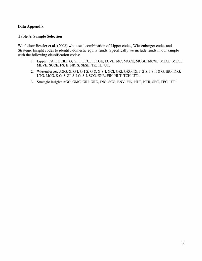
34
Data Appendix
Table A. Sample Selection
We follow Bessler et al. (2008) who use a combination of Lipper codes, Wiesenberger codes and
Strategic Insight codes to identify domestic equity funds. Specifically we include funds in our sample
with the following classification codes:
1. Lipper: CA, EI, EIEI, G, GI, I, LCCE, LCGE, LCVE, MC, MCCE, MCGE, MCVE, MLCE, MLGE,
MLVE, SCCE, FS, H, NR, S, SESE, TK, TL, UT.
2. Wiesenberger: AGG, G, G-I, G-I-S, G-S, G-S-I, GCI, GRI, GRO, IG, I-G-S, I-S, I-S-G, IEQ, ING,
LTG, MCG, S-G, S-GI, S-I-G, S-I, SCG, ENR, FIN, HLT, TCH, UTL.
3. Strategic Insight: AGG, GMC, GRI, GRO, ING, SCG, ENV, FIN, HLT, NTR, SEC, TEC, UTI.
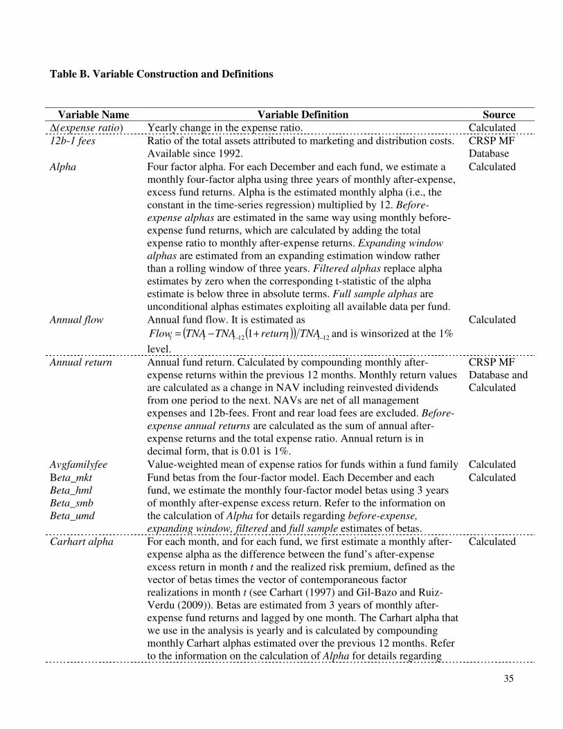
35
Table B. Variable Construction and Definitions
Variable Name Variable Definition Source
∆(expense ratio) Yearly change in the expense ratio. Calculated
12b-1 fees Ratio of the total assets attributed to marketing and distribution costs.
Available since 1992.
CRSP MF
Database
Alpha Four factor alpha. For each December and each fund, we estimate a
monthly four-factor alpha using three years of monthly after-expense,
excess fund returns. Alpha is the estimated monthly alpha (i.e., the
constant in the time-series regression) multiplied by 12. Before-
expense alphas are estimated in the same way using monthly before-
expense fund returns, which are calculated by adding the total
expense ratio to monthly after-expense returns. Expanding window
alphas are estimated from an expanding estimation window rather
than a rolling window of three years. Filtered alphas replace alpha
estimates by zero when the corresponding t-statistic of the alpha
estimate is below three in absolute terms. Full sample alphas are
unconditional alphas estimates exploiting all available data per fund.
Calculated
Annual flow Annual fund flow. It is estimated as
( )( ) 1212 1−−
+−= ttttt TNAreturnTNATNAFlow and is winsorized at the 1%
level.
Calculated
Annual return
Annual fund return. Calculated by compounding monthly after-
expense returns within the previous 12 months. Monthly return values
are calculated as a change in NAV including reinvested dividends
from one period to the next. NAVs are net of all management
expenses and 12b-fees. Front and rear load fees are excluded. Before-
expense annual returns are calculated as the sum of annual after-
expense returns and the total expense ratio. Annual return is in
decimal form, that is 0.01 is 1%.
CRSP MF
Database and
Calculated
Avgfamilyfee Value-weighted mean of expense ratios for funds within a fund family Calculated
Beta_mkt
Beta_hml
Beta_smb
Beta_umd
Fund betas from the four-factor model. Each December and each
fund, we estimate the monthly four-factor model betas using 3 years
of monthly after-expense excess return. Refer to the information on
the calculation of Alpha for details regarding before-expense,
expanding window, filtered and full sample estimates of betas.
Calculated
Carhart alpha For each month, and for each fund, we first estimate a monthly after-
expense alpha as the difference between the fund’s after-expense
excess return in month t and the realized risk premium, defined as the
vector of betas times the vector of contemporaneous factor
realizations in month t (see Carhart (1997) and Gil-Bazo and Ruiz-
Verdu (2009)). Betas are estimated from 3 years of monthly after-
expense fund returns and lagged by one month. The Carhart alpha that
we use in the analysis is yearly and is calculated by compounding
monthly Carhart alphas estimated over the previous 12 months. Refer
to the information on the calculation of Alpha for details regarding
Calculated

36
Variable Name Variable Definition Source
before-expense, expanding window, filtered and full sample estimates
of Carhart alphas. Carhart alpha is in decimal form, that is 0.01 is 1%.
Expense ratio Annual ratio of total investment that shareholders pay for the fund’s
operating expenses, which include 12b-1 fees.
CRSP MF
Database
Family1 dummy
Family10 dummy
Family100 dummy
Family250 dummy
A dummy variable equal to 1, 0 else, if a fund is part of a
management company with more than 1 (10) [100] {250} funds
associated with it. The standard case in our analysis is Family100
dummy.
Calculated.
First expense ratio Total yearly expense ratio in the year when the fund was initiated. Calculated
Flow
autocorrelation
This is the autocorrelation of monthly fund flows. The flow
autocorrelations is estimated using the entire time series of monthly
flows.
Calculated
Flow-perf
sensitivity
For each fund and each year, we estimate the fund’s flow-
performance sensitivity as the coefficient of lagged monthly
performance in a regression that explains monthly flows. The
regression starts with 3 years of monthly data and uses an expanding
window.
Calculated
Front load Front loads for investments represent maximum sales charges. They
often change with the level of investment. The front load value is the
equal weighted average of all front loads charged by a fund across
different investment levels.
CRSP MF
Database
Fund age Age of fund calculated as the difference between current year and
year of fund initiation.
Calculated
Institutional
dummy
Open dummy
ETF dummy
A dummy variable equal to 1, 0 else, if a fund is an institutional fund,
or open to new investment, or is an ETF.
CRSP MF
Database
ln(MgmtComp
TNA)
The natural log of each December’s sum of total net assets of all
funds belonging to the same management company.
Calculated
ln(TNA) The natural log of total net assets per fund as of December-end. Calculated
Pension Plan
dummy
A dummy variable equal to 1, 0 else, if a fund’s monthly
autocorrelation is in the top decile of all funds.
Calculated
Persistence dummy A dummy variable equal to 1 for a given fund in year t if the fund is
among the top-20% funds with respect to yearly net performance in
years t-1 and t-2. The term “before-expense persistence dummy”
refers to a persistence dummy that is based on gross returns rather
than net returns.
Calculated
R2 For each December and each fund, we estimate the four-factor model
using 3 years of monthly fund returns. Then we collect the adjusted
R2 of these models.
Calculated
Random fee
changes
For each fund and each year, we determine the fraction of positive
and negative fee changes for the fund since its first appearance in the
CRSP Mutual Fund Database. “Random fees changes” is the
minimum value of the frequency of positive and negative fee changes.
Calculated
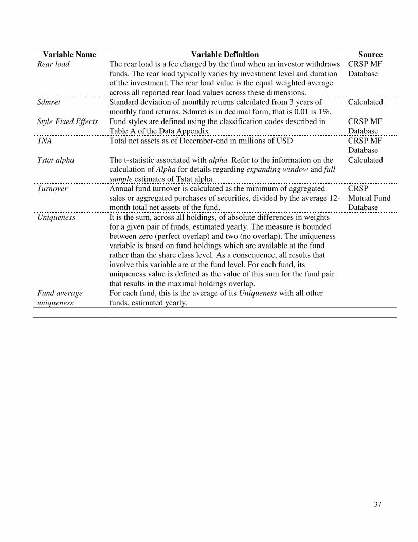
37
Variable Name Variable Definition Source
Rear load The rear load is a fee charged by the fund when an investor withdraws
funds. The rear load typically varies by investment level and duration
of the investment. The rear load value is the equal weighted average
across all reported rear load values across these dimensions.
CRSP MF
Database
Sdmret
Standard deviation of monthly returns calculated from 3 years of
monthly fund returns. Sdmret is in decimal form, that is 0.01 is 1%.
Calculated
Style Fixed Effects Fund styles are defined using the classification codes described in
Table A of the Data Appendix.
CRSP MF
Database
TNA Total net assets as of December-end in millions of USD. CRSP MF
Database
Tstat alpha The t-statistic associated with alpha. Refer to the information on the
calculation of Alpha for details regarding expanding window and full
sample estimates of Tstat alpha.
Calculated
Turnover Annual fund turnover is calculated as the minimum of aggregated
sales or aggregated purchases of securities, divided by the average 12-
month total net assets of the fund.
CRSP
Mutual Fund
Database
Uniqueness It is the sum, across all holdings, of absolute differences in weights
for a given pair of funds, estimated yearly. The measure is bounded
between zero (perfect overlap) and two (no overlap). The uniqueness
variable is based on fund holdings which are available at the fund
rather than the share class level. As a consequence, all results that
involve this variable are at the fund level. For each fund, its
uniqueness value is defined as the value of this sum for the fund pair
that results in the maximal holdings overlap.
Fund average
uniqueness
For each fund, this is the average of its Uniqueness with all other
funds, estimated yearly.
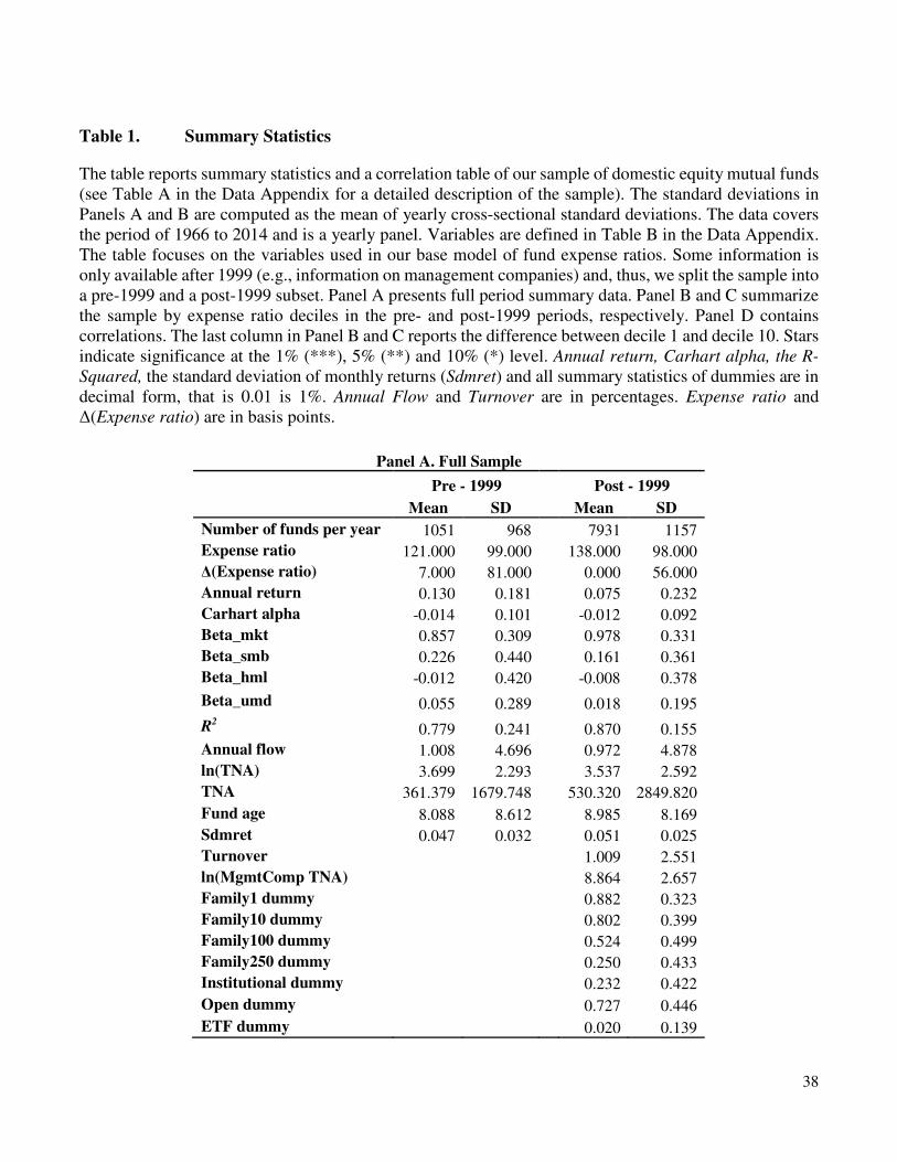
38
Table 1. Summary Statistics
The table reports summary statistics and a correlation table of our sample of domestic equity mutual funds
(see Table A in the Data Appendix for a detailed description of the sample). The standard deviations in
Panels A and B are computed as the mean of yearly cross-sectional standard deviations. The data covers
the period of 1966 to 2014 and is a yearly panel. Variables are defined in Table B in the Data Appendix.
The table focuses on the variables used in our base model of fund expense ratios. Some information is
only available after 1999 (e.g., information on management companies) and, thus, we split the sample into
a pre-1999 and a post-1999 subset. Panel A presents full period summary data. Panel B and C summarize
the sample by expense ratio deciles in the pre- and post-1999 periods, respectively. Panel D contains
correlations. The last column in Panel B and C reports the difference between decile 1 and decile 10. Stars
indicate significance at the 1% (***), 5% (**) and 10% (*) level. Annual return, Carhart alpha, the R-
Squared, the standard deviation of monthly returns (Sdmret) and all summary statistics of dummies are in
decimal form, that is 0.01 is 1%. Annual Flow and Turnover are in percentages. Expense ratio and
Δ(Expense ratio) are in basis points.
Panel A. Full Sample
Pre - 1999 Post - 1999
Mean SD Mean SD
Number of funds per year 1051 968 7931 1157
Expense ratio 121.000 99.000 138.000 98.000
Δ(Expense ratio) 7.000 81.000 0.000 56.000
Annual return 0.130 0.181 0.075 0.232
Carhart alpha -0.014 0.101 -0.012 0.092
Beta_mkt 0.857 0.309 0.978 0.331
Beta_smb 0.226 0.440 0.161 0.361
Beta_hml -0.012 0.420 -0.008 0.378
Beta_umd 0.055 0.289 0.018 0.195
R2 0.779 0.241 0.870 0.155
Annual flow 1.008 4.696 0.972 4.878
ln(TNA) 3.699 2.293 3.537 2.592
TNA 361.379 1679.748 530.320 2849.820
Fund age 8.088 8.612 8.985 8.169
Sdmret 0.047 0.032 0.051 0.025
Turnover 1.009 2.551
ln(MgmtComp TNA) 8.864 2.657
Family1 dummy 0.882 0.323
Family10 dummy 0.802 0.399
Family100 dummy 0.524 0.499
Family250 dummy 0.250 0.433
Institutional dummy 0.232 0.422
Open dummy 0.727 0.446
ETF dummy 0.020 0.139
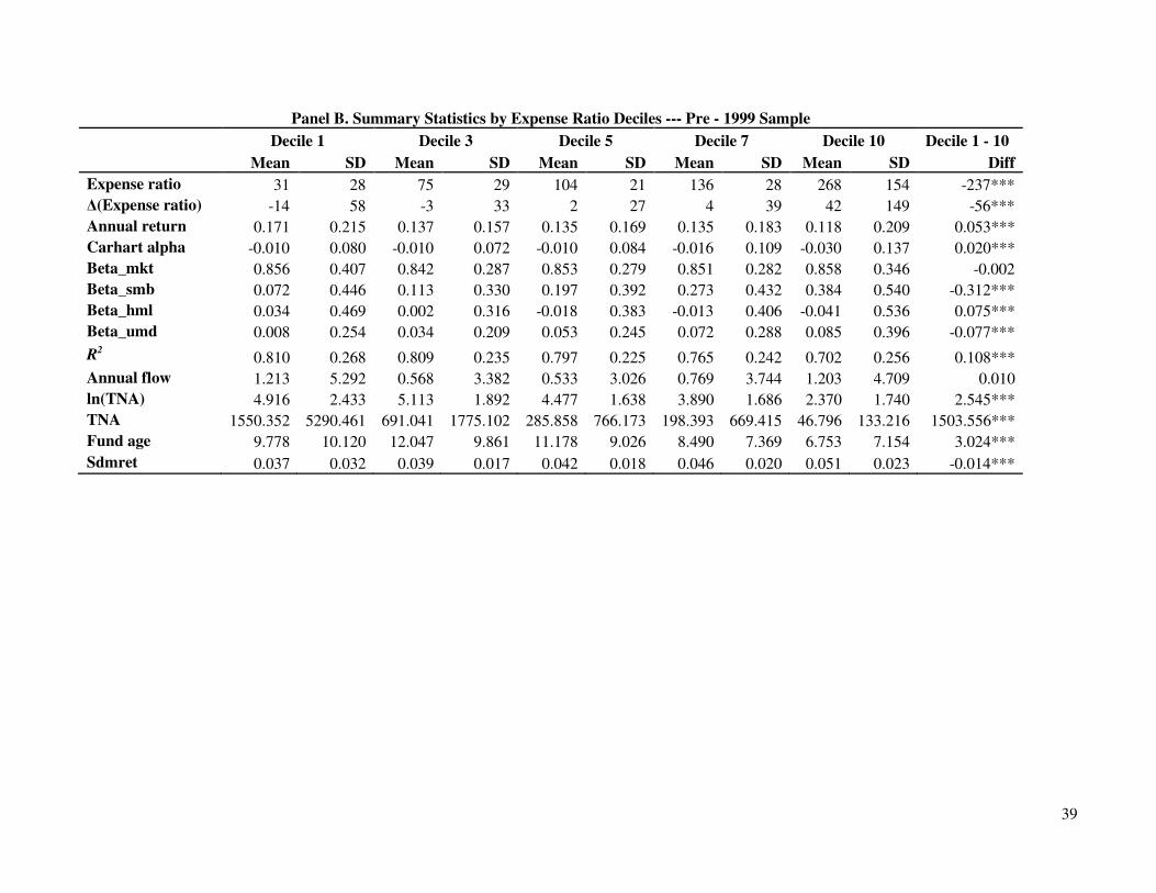
39
Panel B. Summary Statistics by Expense Ratio Deciles --- Pre - 1999 Sample
Decile 1 Decile 3 Decile 5 Decile 7 Decile 10 Decile 1 - 10
Mean SD Mean SD Mean SD Mean SD Mean SD Diff
Expense ratio 31 28 75 29 104 21 136 28 268 154 -237***
Δ(Expense ratio) -14 58 -3 33 2 27 4 39 42 149 -56***
Annual return 0.171 0.215 0.137 0.157 0.135 0.169 0.135 0.183 0.118 0.209 0.053***
Carhart alpha -0.010 0.080 -0.010 0.072 -0.010 0.084 -0.016 0.109 -0.030 0.137 0.020***
Beta_mkt 0.856 0.407 0.842 0.287 0.853 0.279 0.851 0.282 0.858 0.346 -0.002
Beta_smb 0.072 0.446 0.113 0.330 0.197 0.392 0.273 0.432 0.384 0.540 -0.312***
Beta_hml 0.034 0.469 0.002 0.316 -0.018 0.383 -0.013 0.406 -0.041 0.536 0.075***
Beta_umd 0.008 0.254 0.034 0.209 0.053 0.245 0.072 0.288 0.085 0.396 -0.077***
R2 0.810 0.268 0.809 0.235 0.797 0.225 0.765 0.242 0.702 0.256 0.108***
Annual flow 1.213 5.292 0.568 3.382 0.533 3.026 0.769 3.744 1.203 4.709 0.010
ln(TNA) 4.916 2.433 5.113 1.892 4.477 1.638 3.890 1.686 2.370 1.740 2.545***
TNA 1550.352 5290.461 691.041 1775.102 285.858 766.173 198.393 669.415 46.796 133.216 1503.556***
Fund age 9.778 10.120 12.047 9.861 11.178 9.026 8.490 7.369 6.753 7.154 3.024***
Sdmret 0.037 0.032 0.039 0.017 0.042 0.018 0.046 0.020 0.051 0.023 -0.014***
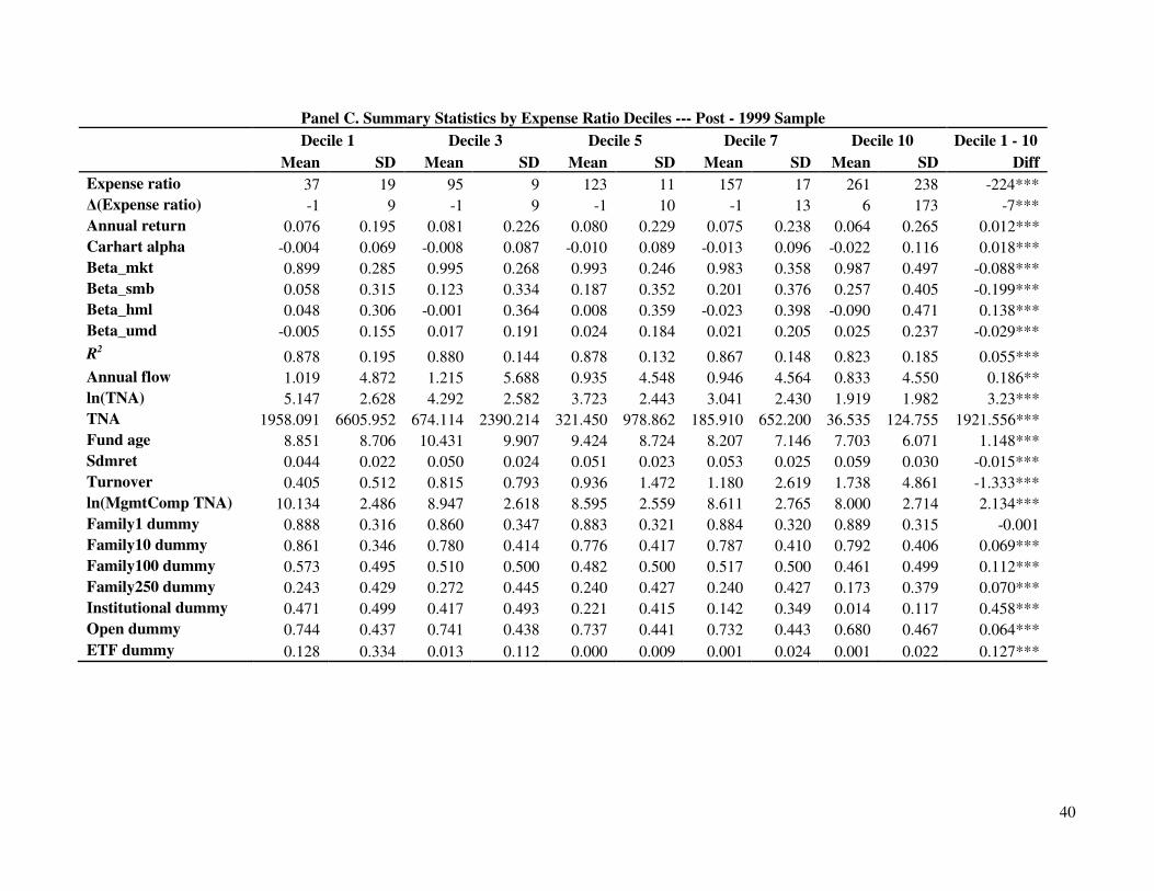
40
Panel C. Summary Statistics by Expense Ratio Deciles --- Post - 1999 Sample
Decile 1 Decile 3 Decile 5 Decile 7 Decile 10 Decile 1 - 10
Mean SD Mean SD Mean SD Mean SD Mean SD Diff
Expense ratio 37 19 95 9 123 11 157 17 261 238 -224***
Δ(Expense ratio) -1 9 -1 9 -1 10 -1 13 6 173 -7***
Annual return 0.076 0.195 0.081 0.226 0.080 0.229 0.075 0.238 0.064 0.265 0.012***
Carhart alpha -0.004 0.069 -0.008 0.087 -0.010 0.089 -0.013 0.096 -0.022 0.116 0.018***
Beta_mkt 0.899 0.285 0.995 0.268 0.993 0.246 0.983 0.358 0.987 0.497 -0.088***
Beta_smb 0.058 0.315 0.123 0.334 0.187 0.352 0.201 0.376 0.257 0.405 -0.199***
Beta_hml 0.048 0.306 -0.001 0.364 0.008 0.359 -0.023 0.398 -0.090 0.471 0.138***
Beta_umd -0.005 0.155 0.017 0.191 0.024 0.184 0.021 0.205 0.025 0.237 -0.029***
R2 0.878 0.195 0.880 0.144 0.878 0.132 0.867 0.148 0.823 0.185 0.055***
Annual flow 1.019 4.872 1.215 5.688 0.935 4.548 0.946 4.564 0.833 4.550 0.186**
ln(TNA) 5.147 2.628 4.292 2.582 3.723 2.443 3.041 2.430 1.919 1.982 3.23***
TNA 1958.091 6605.952 674.114 2390.214 321.450 978.862 185.910 652.200 36.535 124.755 1921.556***
Fund age 8.851 8.706 10.431 9.907 9.424 8.724 8.207 7.146 7.703 6.071 1.148***
Sdmret 0.044 0.022 0.050 0.024 0.051 0.023 0.053 0.025 0.059 0.030 -0.015***
Turnover 0.405 0.512 0.815 0.793 0.936 1.472 1.180 2.619 1.738 4.861 -1.333***
ln(MgmtComp TNA) 10.134 2.486 8.947 2.618 8.595 2.559 8.611 2.765 8.000 2.714 2.134***
Family1 dummy 0.888 0.316 0.860 0.347 0.883 0.321 0.884 0.320 0.889 0.315 -0.001
Family10 dummy 0.861 0.346 0.780 0.414 0.776 0.417 0.787 0.410 0.792 0.406 0.069***
Family100 dummy 0.573 0.495 0.510 0.500 0.482 0.500 0.517 0.500 0.461 0.499 0.112***
Family250 dummy 0.243 0.429 0.272 0.445 0.240 0.427 0.240 0.427 0.173 0.379 0.070***
Institutional dummy 0.471 0.499 0.417 0.493 0.221 0.415 0.142 0.349 0.014 0.117 0.458***
Open dummy 0.744 0.437 0.741 0.438 0.737 0.441 0.732 0.443 0.680 0.467 0.064***
ETF dummy 0.128 0.334 0.013 0.112 0.000 0.009 0.001 0.024 0.001 0.022 0.127***
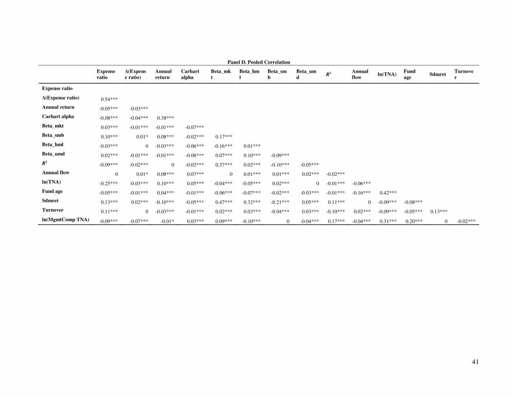
41
Panel D. Pooled Correlation
Expense
ratio
Δ(Expens
e ratio)
Annual
return
Carhart
alpha
Beta_mk
t
Beta_hm
l
Beta_sm
b
Beta_um
d R
2
Annual
flow ln(TNA)
Fund
age Sdmret
Turnove
r
Expense ratio
Δ(Expense ratio) 0.54***
Annual return -0.05*** -0.03***
Carhart alpha -0.08*** -0.04*** 0.38***
Beta_mkt 0.03*** -0.01*** -0.01*** -0.07***
Beta_smb 0.10*** 0.01* 0.08*** -0.02*** 0.17***
Beta_hml -0.03*** 0 -0.03*** -0.06*** -0.16*** 0.01***
Beta_umd 0.02*** -0.01*** -0.01*** -0.08*** 0.07*** 0.10*** -0.09***
R2 -0.09*** -0.02*** 0 -0.02*** 0.37*** 0.02*** -0.10*** -0.05***
Annual flow 0 0.01* 0.08*** 0.07*** 0 0.01*** 0.01*** 0.02*** -0.02***
ln(TNA) -0.25*** -0.03*** 0.10*** 0.05*** -0.04*** -0.05*** 0.02*** 0 -0.01*** -0.06***
Fund age -0.05*** -0.01*** 0.04*** -0.01*** -0.06*** -0.07*** -0.02*** -0.03*** -0.01*** -0.16*** 0.42***
Sdmret 0.13*** 0.02*** -0.10*** -0.05*** 0.47*** 0.32*** -0.21*** 0.05*** 0.11*** 0 -0.09*** -0.08***
Turnover 0.11*** 0 -0.03*** -0.01*** 0.02*** 0.03*** -0.04*** 0.03*** -0.10*** 0.02*** -0.09*** -0.05*** 0.13***
ln(MgmtComp TNA) -0.09*** -0.07*** -0.01* 0.03*** 0.09*** -0.10*** 0 -0.04*** 0.17*** -0.04*** 0.31*** 0.20*** 0 -0.02***
42
Table 2. Base-Case Fund Expense Regressions
The table reports results of Fama-MacBeth regressions in which yearly expense ratios are regressed on lagged fund characteristics (see Table
A in the Data Appendix for a detailed description of the sample). The data covers the period of 1966 to 2014 and is a yearly panel. Variables
are defined in Table B in the Data Appendix. All variables are lagged by one year. Expense ratio (the dependent variable in all regressions) is
in basis points. We split the sample into pre-and post-1999 subperiods since information on management companies is only available after
1999. The specifications reported in this table represent the base-case specifications. Beta estimates are time series averages of cross-sectional
regression betas obtained from annual cross-sectional regressions. We perform the regressions on the full sample of mutual funds and for the
largest and smallest quintile of annually ranked TNA funds. Panel A reports the regression results. We standardize all the independent variables
to mean 0 and standard deviation 1 using the full-sample mean of each variable’s yearly cross-sectional mean and SD. In Panel B, in column
(1) we report the time-series average of the cross-sectional mean, in column (2) the time-series standard deviation of the cross-sectional mean,
and in column (3), the time-series average of the cross-sectional SD that are used to standardize the independent variables in panel A.
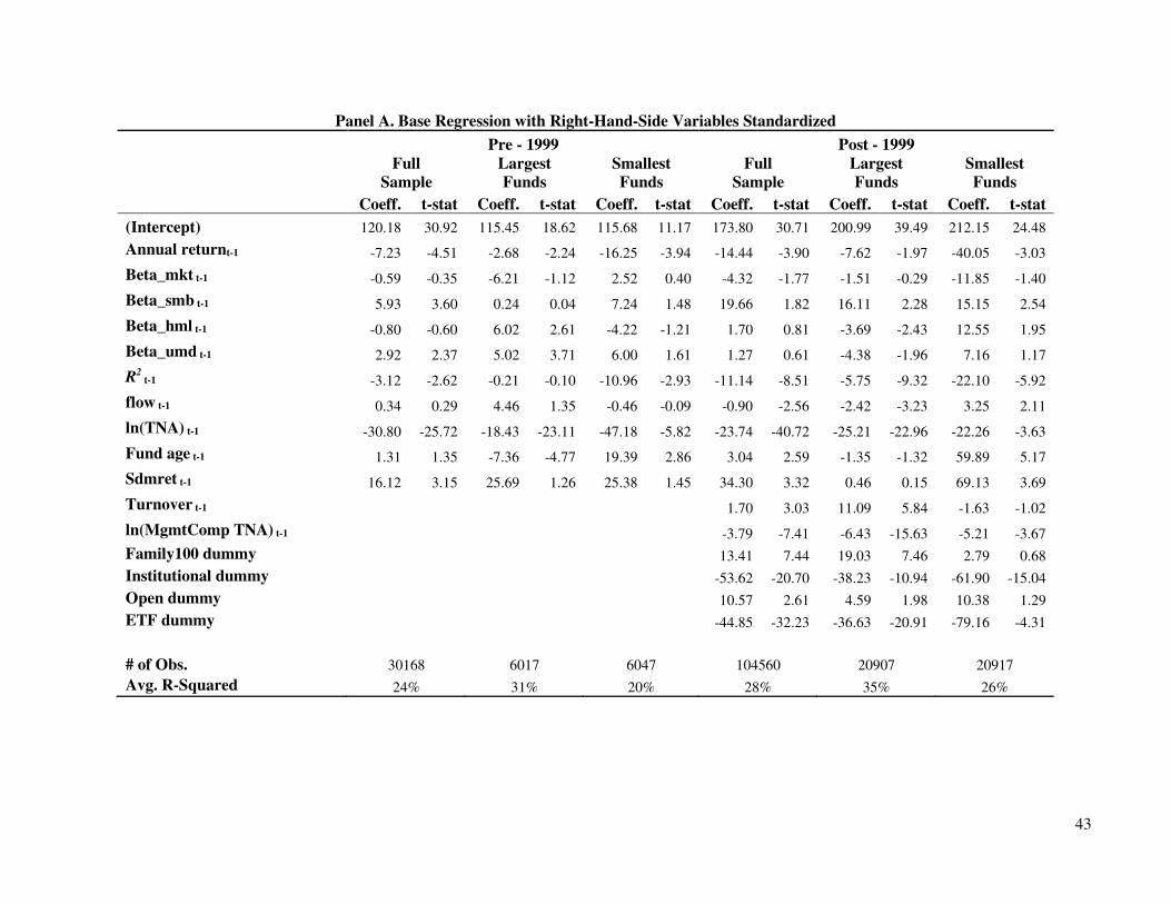
43
Panel A. Base Regression with Right-Hand-Side Variables Standardized
Pre - 1999 Post - 1999
Full
Sample
Largest
Funds
Smallest
Funds
Full
Sample
Largest
Funds
Smallest
Funds
Coeff. t-stat Coeff. t-stat Coeff. t-stat Coeff. t-stat Coeff. t-stat Coeff. t-stat
(Intercept) 120.18 30.92 115.45 18.62 115.68 11.17 173.80 30.71 200.99 39.49 212.15 24.48
Annual returnt-1 -7.23 -4.51 -2.68 -2.24 -16.25 -3.94 -14.44 -3.90 -7.62 -1.97 -40.05 -3.03
Beta_mkt t-1 -0.59 -0.35 -6.21 -1.12 2.52 0.40 -4.32 -1.77 -1.51 -0.29 -11.85 -1.40
Beta_smb t-1 5.93 3.60 0.24 0.04 7.24 1.48 19.66 1.82 16.11 2.28 15.15 2.54
Beta_hml t-1 -0.80 -0.60 6.02 2.61 -4.22 -1.21 1.70 0.81 -3.69 -2.43 12.55 1.95
Beta_umd t-1 2.92 2.37 5.02 3.71 6.00 1.61 1.27 0.61 -4.38 -1.96 7.16 1.17
R2 t-1 -3.12 -2.62 -0.21 -0.10 -10.96 -2.93 -11.14 -8.51 -5.75 -9.32 -22.10 -5.92
flow t-1 0.34 0.29 4.46 1.35 -0.46 -0.09 -0.90 -2.56 -2.42 -3.23 3.25 2.11
ln(TNA) t-1 -30.80 -25.72 -18.43 -23.11 -47.18 -5.82 -23.74 -40.72 -25.21 -22.96 -22.26 -3.63
Fund age t-1 1.31 1.35 -7.36 -4.77 19.39 2.86 3.04 2.59 -1.35 -1.32 59.89 5.17
Sdmret t-1 16.12 3.15 25.69 1.26 25.38 1.45 34.30 3.32 0.46 0.15 69.13 3.69
Turnover t-1 1.70 3.03 11.09 5.84 -1.63 -1.02
ln(MgmtComp TNA) t-1 -3.79 -7.41 -6.43 -15.63 -5.21 -3.67
Family100 dummy 13.41 7.44 19.03 7.46 2.79 0.68
Institutional dummy -53.62 -20.70 -38.23 -10.94 -61.90 -15.04
Open dummy 10.57 2.61 4.59 1.98 10.38 1.29
ETF dummy -44.85 -32.23 -36.63 -20.91 -79.16 -4.31
# of Obs. 30168 6017 6047 104560 20907 20917
Avg. R-Squared 24% 31% 20% 28% 35% 26%
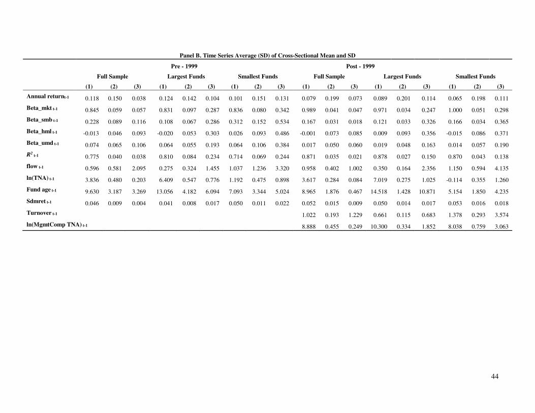
44
Panel B. Time Series Average (SD) of Cross-Sectional Mean and SD
Pre - 1999 Post - 1999
Full Sample Largest Funds Smallest Funds Full Sample Largest Funds Smallest Funds
(1) (2) (3) (1) (2) (3) (1) (2) (3) (1) (2) (3) (1) (2) (3) (1) (2) (3)
Annual returnt-1 0.118 0.150 0.038 0.124 0.142 0.104 0.101 0.151 0.131 0.079 0.199 0.073 0.089 0.201 0.114 0.065 0.198 0.111
Beta_mkt t-1 0.845 0.059 0.057 0.831 0.097 0.287 0.836 0.080 0.342 0.989 0.041 0.047 0.971 0.034 0.247 1.000 0.051 0.298
Beta_smb t-1 0.228 0.089 0.116 0.108 0.067 0.286 0.312 0.152 0.534 0.167 0.031 0.018 0.121 0.033 0.326 0.166 0.034 0.365
Beta_hml t-1 -0.013 0.046 0.093 -0.020 0.053 0.303 0.026 0.093 0.486 -0.001 0.073 0.085 0.009 0.093 0.356 -0.015 0.086 0.371
Beta_umd t-1 0.074 0.065 0.106 0.064 0.055 0.193 0.064 0.106 0.384 0.017 0.050 0.060 0.019 0.048 0.163 0.014 0.057 0.190
R2 t-1 0.775 0.040 0.038 0.810 0.084 0.234 0.714 0.069 0.244 0.871 0.035 0.021 0.878 0.027 0.150 0.870 0.043 0.138
flow t-1 0.596 0.581 2.095 0.275 0.324 1.455 1.037 1.236 3.320 0.958 0.402 1.002 0.350 0.164 2.356 1.150 0.594 4.135
ln(TNA) t-1 3.836 0.480 0.203 6.409 0.547 0.776 1.192 0.475 0.898 3.617 0.284 0.084 7.019 0.275 1.025 -0.114 0.355 1.260
Fund age t-1 9.630 3.187 3.269 13.056 4.182 6.094 7.093 3.344 5.024 8.965 1.876 0.467 14.518 1.428 10.871 5.154 1.850 4.235
Sdmret t-1 0.046 0.009 0.004 0.041 0.008 0.017 0.050 0.011 0.022 0.052 0.015 0.009 0.050 0.014 0.017 0.053 0.016 0.018
Turnover t-1 1.022 0.193 1.229 0.661 0.115 0.683 1.378 0.293 3.574
ln(MgmtComp TNA) t-1 8.888 0.455 0.249 10.300 0.334 1.852 8.038 0.759 3.063
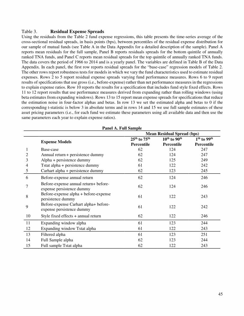
45
Table 3. Residual Expense Spreads Using the residuals from the Table 2 fund expense regressions, this table presents the time-series average of the
cross-sectional residual spreads, in basis points (bps), between percentiles of the residual expense distribution for
our sample of mutual funds (see Table A in the Data Appendix for a detailed description of the sample). Panel A
reports mean residuals for the full sample, Panel B reports residuals spreads for the bottom quintile of annually
ranked TNA funds, and Panel C reports mean residual spreads for the top quintile of annually ranked TNA funds.
The data covers the period of 1966 to 2014 and is a yearly panel. The variables are defined in Table B of the Data
Appendix. In each panel, the first row reports residual spreads for the “base-case” regression models of Table 2.
The other rows report robustness tests for models in which we vary the fund characteristics used to estimate residual
expenses. Rows 2 to 5 report residual expense spreads varying fund performance measures. Rows 6 to 9 report
results of specifications that use gross (i.e., before-expense) rather than net performance measures in the regressions
to explain expense ratios. Row 10 reports the results for a specification that includes fund style fixed effects. Rows
11 to 12 report results that use performance measures derived from expanding rather than rolling windows (using
beta estimates from expanding windows). Rows 13 to 15 report mean expense spreads for specifications that reduce
the estimation noise in four-factor alphas and betas. In row 13 we set the estimated alpha and betas to 0 if the
corresponding t-statistic is below 3 in absolute terms and in rows 14 and 15 we use full sample estimates of these
asset pricing parameters (i.e., for each fund we estimate these parameters using all available data and then use the
same parameters each year to explain expense ratios).
Panel A. Full Sample
Mean Residual Spread (bps)
Expense Models 25th to 75th
Percentile
10th to 90th
Percentile
1th to 99th
Percentile
1 Base-case 62 124 247
2 Annual return + persistence dummy 62 124 247
3 Alpha + persistence dummy 62 125 249
4 Tstat alpha + persistence dummy 61 122 242
5 Carhart alpha + persistence dummy 62 123 245
6 Before-expense annual return 62 124 246
7 Before-expense annual return+ before-
expense persistence dummy 62 124 246
8 Before-expense alpha + before-expense
persistence dummy 61 122 243
9 Before-expense Carhart alpha+ before-
expense persistence dummy 61 122 242
10 Style fixed effects + annual return 62 122 246
11 Expanding window alpha 61 123 244
12 Expanding window Tstat alpha 61 122 243
13 Filtered alpha 61 123 251
14 Full Sample alpha 62 123 244
15 Full sample Tstat alpha 62 122 243
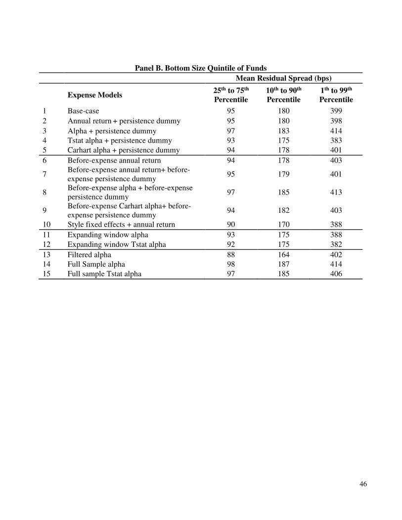
46
Panel B. Bottom Size Quintile of Funds
Mean Residual Spread (bps)
Expense Models 25th to 75th
Percentile
10th to 90th
Percentile
1th to 99th
Percentile
1 Base-case 95 180 399
2 Annual return + persistence dummy 95 180 398
3 Alpha + persistence dummy 97 183 414
4 Tstat alpha + persistence dummy 93 175 383
5 Carhart alpha + persistence dummy 94 178 401
6 Before-expense annual return 94 178 403
7 Before-expense annual return+ before-
expense persistence dummy 95 179 401
8 Before-expense alpha + before-expense
persistence dummy 97 185 413
9 Before-expense Carhart alpha+ before-
expense persistence dummy 94 182 403
10 Style fixed effects + annual return 90 170 388
11 Expanding window alpha 93 175 388
12 Expanding window Tstat alpha 92 175 382
13 Filtered alpha 88 164 402
14 Full Sample alpha 98 187 414
15 Full sample Tstat alpha 97 185 406
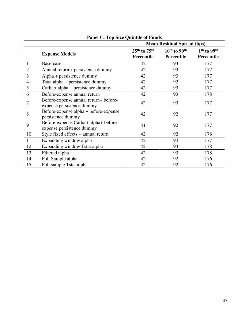
47
Panel C. Top Size Quintile of Funds
Mean Residual Spread (bps)
Expense Models 25th to 75th
Percentile
10th to 90th
Percentile
1th to 99th
Percentile
1 Base-case 42 93 177
2 Annual return + persistence dummy 42 93 177
3 Alpha + persistence dummy 42 93 177
4 Tstat alpha + persistence dummy 42 92 177
5 Carhart alpha + persistence dummy 42 93 177
6 Before-expense annual return 42 93 178
7 Before-expense annual return+ before-
expense persistence dummy 42 93 177
8 Before-expense alpha + before-expense
persistence dummy 42 92 177
9 Before-expense Carhart alpha+ before-
expense persistence dummy 41 92 177
10 Style fixed effects + annual return 42 92 176
11 Expanding window alpha 42 94 177
12 Expanding window Tstat alpha 42 93 178
13 Filtered alpha 42 93 178
14 Full Sample alpha 42 92 176
15 Full sample Tstat alpha 42 92 176
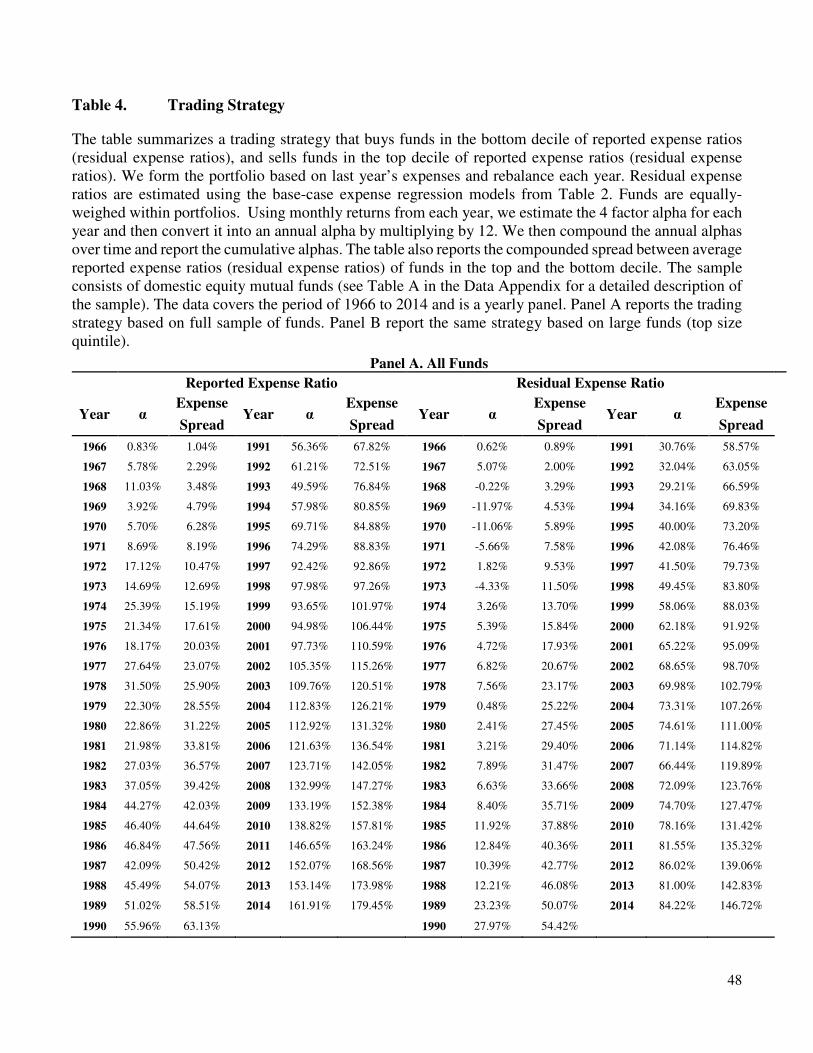
48
Table 4. Trading Strategy
The table summarizes a trading strategy that buys funds in the bottom decile of reported expense ratios
(residual expense ratios), and sells funds in the top decile of reported expense ratios (residual expense
ratios). We form the portfolio based on last year’s expenses and rebalance each year. Residual expense
ratios are estimated using the base-case expense regression models from Table 2. Funds are equally-
weighed within portfolios. Using monthly returns from each year, we estimate the 4 factor alpha for each
year and then convert it into an annual alpha by multiplying by 12. We then compound the annual alphas
over time and report the cumulative alphas. The table also reports the compounded spread between average
reported expense ratios (residual expense ratios) of funds in the top and the bottom decile. The sample
consists of domestic equity mutual funds (see Table A in the Data Appendix for a detailed description of
the sample). The data covers the period of 1966 to 2014 and is a yearly panel. Panel A reports the trading
strategy based on full sample of funds. Panel B report the same strategy based on large funds (top size
quintile).
Panel A. All Funds
Reported Expense Ratio Residual Expense Ratio
Year α Expense
Year α Expense
Year α Expense
Year α Expense
Spread Spread Spread Spread
1966 0.83% 1.04% 1991 56.36% 67.82% 1966 0.62% 0.89% 1991 30.76% 58.57%
1967 5.78% 2.29% 1992 61.21% 72.51% 1967 5.07% 2.00% 1992 32.04% 63.05%
1968 11.03% 3.48% 1993 49.59% 76.84% 1968 -0.22% 3.29% 1993 29.21% 66.59%
1969 3.92% 4.79% 1994 57.98% 80.85% 1969 -11.97% 4.53% 1994 34.16% 69.83%
1970 5.70% 6.28% 1995 69.71% 84.88% 1970 -11.06% 5.89% 1995 40.00% 73.20%
1971 8.69% 8.19% 1996 74.29% 88.83% 1971 -5.66% 7.58% 1996 42.08% 76.46%
1972 17.12% 10.47% 1997 92.42% 92.86% 1972 1.82% 9.53% 1997 41.50% 79.73%
1973 14.69% 12.69% 1998 97.98% 97.26% 1973 -4.33% 11.50% 1998 49.45% 83.80%
1974 25.39% 15.19% 1999 93.65% 101.97% 1974 3.26% 13.70% 1999 58.06% 88.03%
1975 21.34% 17.61% 2000 94.98% 106.44% 1975 5.39% 15.84% 2000 62.18% 91.92%
1976 18.17% 20.03% 2001 97.73% 110.59% 1976 4.72% 17.93% 2001 65.22% 95.09%
1977 27.64% 23.07% 2002 105.35% 115.26% 1977 6.82% 20.67% 2002 68.65% 98.70%
1978 31.50% 25.90% 2003 109.76% 120.51% 1978 7.56% 23.17% 2003 69.98% 102.79%
1979 22.30% 28.55% 2004 112.83% 126.21% 1979 0.48% 25.22% 2004 73.31% 107.26%
1980 22.86% 31.22% 2005 112.92% 131.32% 1980 2.41% 27.45% 2005 74.61% 111.00%
1981 21.98% 33.81% 2006 121.63% 136.54% 1981 3.21% 29.40% 2006 71.14% 114.82%
1982 27.03% 36.57% 2007 123.71% 142.05% 1982 7.89% 31.47% 2007 66.44% 119.89%
1983 37.05% 39.42% 2008 132.99% 147.27% 1983 6.63% 33.66% 2008 72.09% 123.76%
1984 44.27% 42.03% 2009 133.19% 152.38% 1984 8.40% 35.71% 2009 74.70% 127.47%
1985 46.40% 44.64% 2010 138.82% 157.81% 1985 11.92% 37.88% 2010 78.16% 131.42%
1986 46.84% 47.56% 2011 146.65% 163.24% 1986 12.84% 40.36% 2011 81.55% 135.32%
1987 42.09% 50.42% 2012 152.07% 168.56% 1987 10.39% 42.77% 2012 86.02% 139.06%
1988 45.49% 54.07% 2013 153.14% 173.98% 1988 12.21% 46.08% 2013 81.00% 142.83%
1989 51.02% 58.51% 2014 161.91% 179.45% 1989 23.23% 50.07% 2014 84.22% 146.72%
1990 55.96% 63.13% 1990 27.97% 54.42%
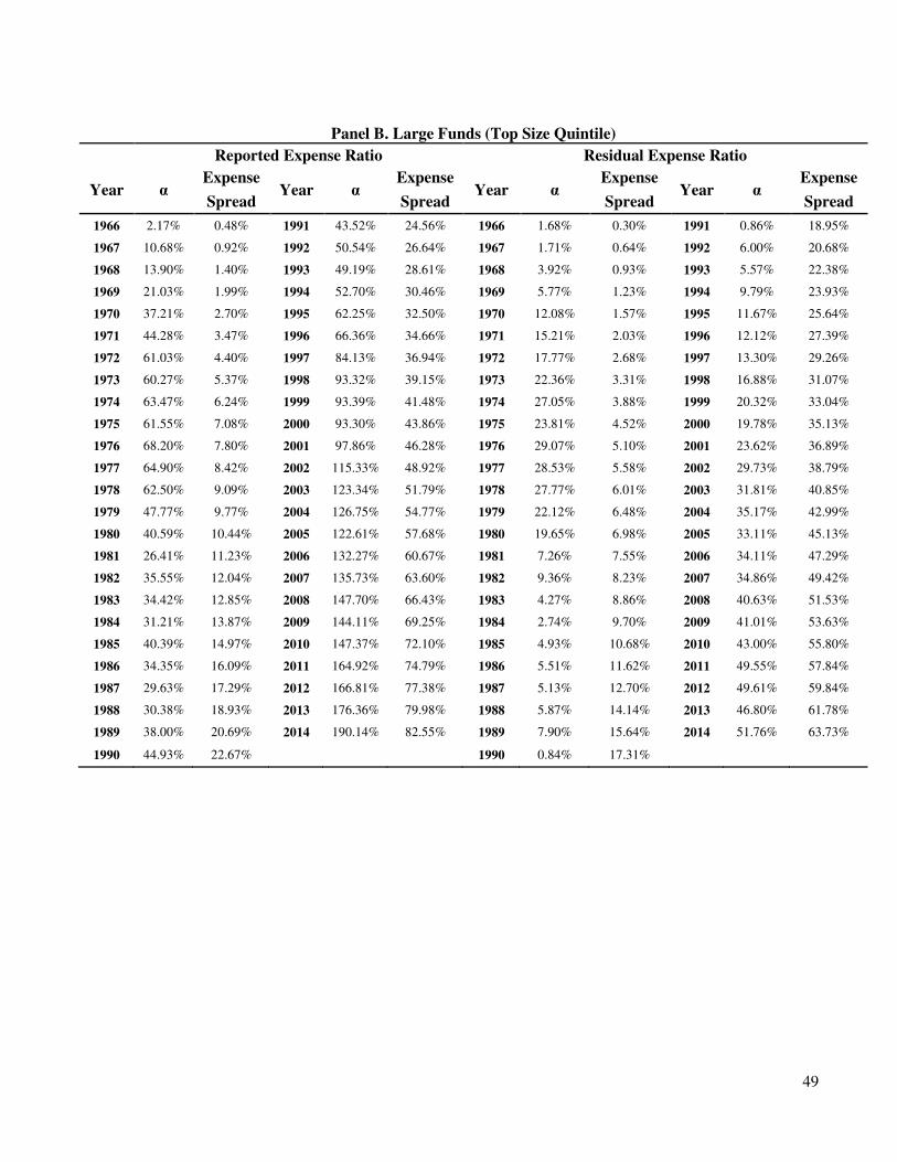
49
Panel B. Large Funds (Top Size Quintile)
Reported Expense Ratio Residual Expense Ratio
Year α Expense
Year α Expense
Year α Expense
Year α Expense
Spread Spread Spread Spread
1966 2.17% 0.48% 1991 43.52% 24.56% 1966 1.68% 0.30% 1991 0.86% 18.95%
1967 10.68% 0.92% 1992 50.54% 26.64% 1967 1.71% 0.64% 1992 6.00% 20.68%
1968 13.90% 1.40% 1993 49.19% 28.61% 1968 3.92% 0.93% 1993 5.57% 22.38%
1969 21.03% 1.99% 1994 52.70% 30.46% 1969 5.77% 1.23% 1994 9.79% 23.93%
1970 37.21% 2.70% 1995 62.25% 32.50% 1970 12.08% 1.57% 1995 11.67% 25.64%
1971 44.28% 3.47% 1996 66.36% 34.66% 1971 15.21% 2.03% 1996 12.12% 27.39%
1972 61.03% 4.40% 1997 84.13% 36.94% 1972 17.77% 2.68% 1997 13.30% 29.26%
1973 60.27% 5.37% 1998 93.32% 39.15% 1973 22.36% 3.31% 1998 16.88% 31.07%
1974 63.47% 6.24% 1999 93.39% 41.48% 1974 27.05% 3.88% 1999 20.32% 33.04%
1975 61.55% 7.08% 2000 93.30% 43.86% 1975 23.81% 4.52% 2000 19.78% 35.13%
1976 68.20% 7.80% 2001 97.86% 46.28% 1976 29.07% 5.10% 2001 23.62% 36.89%
1977 64.90% 8.42% 2002 115.33% 48.92% 1977 28.53% 5.58% 2002 29.73% 38.79%
1978 62.50% 9.09% 2003 123.34% 51.79% 1978 27.77% 6.01% 2003 31.81% 40.85%
1979 47.77% 9.77% 2004 126.75% 54.77% 1979 22.12% 6.48% 2004 35.17% 42.99%
1980 40.59% 10.44% 2005 122.61% 57.68% 1980 19.65% 6.98% 2005 33.11% 45.13%
1981 26.41% 11.23% 2006 132.27% 60.67% 1981 7.26% 7.55% 2006 34.11% 47.29%
1982 35.55% 12.04% 2007 135.73% 63.60% 1982 9.36% 8.23% 2007 34.86% 49.42%
1983 34.42% 12.85% 2008 147.70% 66.43% 1983 4.27% 8.86% 2008 40.63% 51.53%
1984 31.21% 13.87% 2009 144.11% 69.25% 1984 2.74% 9.70% 2009 41.01% 53.63%
1985 40.39% 14.97% 2010 147.37% 72.10% 1985 4.93% 10.68% 2010 43.00% 55.80%
1986 34.35% 16.09% 2011 164.92% 74.79% 1986 5.51% 11.62% 2011 49.55% 57.84%
1987 29.63% 17.29% 2012 166.81% 77.38% 1987 5.13% 12.70% 2012 49.61% 59.84%
1988 30.38% 18.93% 2013 176.36% 79.98% 1988 5.87% 14.14% 2013 46.80% 61.78%
1989 38.00% 20.69% 2014 190.14% 82.55% 1989 7.90% 15.64% 2014 51.76% 63.73%
1990 44.93% 22.67% 1990 0.84% 17.31%
50
Table 5. Share Class Aggregation and Expense Dispersion
This table presents the time-series average of the cross-sectional residual spreads, in basis points (bps),
between percentiles of the residual expense distribution for our sample of mutual funds (see Table A in
the Data Appendix for a detailed description of the sample) for share class aggregation. Panel A reports
mean residuals for the full sample, Panel B reports residuals spreads for the bottom quintile of annually
ranked TNA funds, and Panel C reports mean residual spreads for the top quintile of annually ranked TNA
funds. The sample period covers 1980 to 2014. Row 1 in each panel reports the results from the base-case
specification in which we do not aggregate across share classes. Rows 2-4 report results for samples in
which we aggregate share classes using three different aggregation schemes: equal-weighting
(specification 2), value-weighting (specification 3) and selection of the largest share class (specification
4).
Panel A. Full Sample
Mean Residual Spread (bps)
25th to 75th Percentile 10th to 90th Percentile 1th to 9th Percentile
No Aggregation 63 125 243
Aggregated Share Classes (EW) 63 126 268
Aggregated Share Classes (VW) 58 122 265
Aggregated Share Classes (Largest) 55 117 266
Panel B. Bottom Quintile of Funds
Mean Residual Spread (bps)
25th to 75th Percentile 10th to 90th Percentile 1th to 9th Percentile
No Aggregation 91 184 386
Aggregated Share Classes (EW) 110 222 492
Aggregated Share Classes (VW) 107 221 490
Aggregated Share Classes (Largest) 107 218 498
Panel C. Top Quintile of Funds
Mean Residual Spread (bps)
25th to 75th Percentile 10th to 90th Percentile 1th to 9th Percentile
No Aggregation 50 101 184
Aggregated Share Classes (EW) 45 89 164
Aggregated Share Classes (VW) 40 79 157
Aggregated Share Classes (Largest) 37 77 158
51
Table 6. Differences in Reported Expense Ratios and Residual Expense Ratios for Holdings-matched Fund Pairs
The table reports mean absolute differences in expense (residual) ratios and spreads of absolute differences in expense (residual) ratios for matched fund
pairs. The matching is based on holdings’ overlap measured in terms of “uniqueness.” For each possible fund pair, we estimate, yearly, the sum, across all
holdings, of absolute differences in weights. For each fund, its uniqueness value is defined as the value of this sum for the fund pair that results in the
maximal holdings overlap. The uniqueness measure is bounded between zero (perfect overlap) and two (no overlap). We refer to this sample of matched
fund pairs as the "full pairs sample." We rank uniqueness into quintiles, where quintile 1 contains the most similar fund pairs and quintile 5 contains the least
similar funds pairs. We also define “very similar funds" as the bottom decile of the uniqueness measure. In Panel A we present mean absolute differences
and interquartile ranges (IQR) for fund characteristics of the matched pairs. In Panel B we present mean absolute differences, interquartile ranges and inter-
percentile spreads for reported expense ratios and residual expense ratios, in basis points. The residual expense ratios are from the base-case expense
regression of Table 2. All variables are contemporaneous to the matching of fund pairs.
Panel A. Differences in Fund Characteristics for Matched Pairs
Avg. # of
fund
pairs/year
Uniqueness
(Matching
Criterion)
Annual
return R2 Beta_mkt Beta_smb Beta_hml Beta_umd
Mean IQR Mean IQR Mean IQR Mean IQR Mean IQR Mean IQR Mean IQR
Full pairs
sample 1145.4 1.05 0.58 0.07 0.07 0.08 0.08 0.16 0.18 0.23 0.25 0.2 0.23 0.12 0.13
Very similar
funds 114.94 0.15 0.12 0.03 0.03 0.03 0.02 0.15 0.15 0.08 0.08 0.09 0.09 0.05 0.05
Un
iqu
en
ess
Qu
inti
les
1 229.41 0.32 0.42 0.03 0.03 0.03 0.03 0.13 0.15 0.09 0.1 0.1 0.11 0.06 0.07
2 229.12 0.9 0.34 0.05 0.05 0.05 0.05 0.13 0.14 0.14 0.14 0.16 0.17 0.1 0.1
3 229 1.18 0.2 0.06 0.06 0.06 0.06 0.16 0.16 0.18 0.19 0.2 0.21 0.12 0.12
4 229.12 1.36 0.18 0.08 0.08 0.09 0.09 0.18 0.18 0.27 0.29 0.25 0.26 0.14 0.15
5 228.71 1.49 0.25 0.11 0.12 0.13 0.14 0.22 0.23 0.45 0.52 0.31 0.33 0.18 0.18
52
Panel B. Differences in Expenses for Matched Pairs
Reported Expense Ratio Residual Expense Ratio
Spreads Mean IQR 10th to 90th 1st to
99th Mean IQR
10th
to
90th
1st to
99th
Full pairs
sample 49 54 103 219 46 47 94 206
Very similar
funds 41 48 94 174 38 41 84 167
Un
iqu
en
ess
Qu
inti
les
1 42 49 101 176 40 41 83 172
2 43 51 98 192 40 43 84 176
3 47 52 98 204 45 48 93 190
4 51 55 104 240 50 52 104 214
5 63 57 111 321 56 53 105 274
53
Table 7. Testing Explanations of Residual Expense Spreads
The table reports results for tests of various hypotheses formulated to explain the dispersion in mutual fund expenses. Panel A reports means
and standard deviations of the variables used to test the hypotheses, sorted by reported expense ratio deciles. The last column in Panel A reports
the difference between decile 1 and decile 10 characteristics. Stars indicate significance at the 1% (***), 5% (**) and 10% (*) level. Panel B
(pre-1999) and C (post-1999) report coefficients of on these variables when they are added individually or jointly to the base-case expense
regressions from Table 2. We standardize all the independent variables to mean 0 and standard deviation 1 using the full-sample mean of each
variable’s yearly cross-sectional mean and SD. Panel D reports mean residual expense spreads for the full sample and for the bottom and top
quintile of annually ranked TNA funds after including the hypothesis variables individually or jointly in the expense regressions. In Panel D we
report the spreads for 3 periods: Pre-1999, Post-1999, and Full Period. Variables are defined in Table B in the Data Appendix. All variables are
measured at the share class level, except for fund average uniqueness (i.e., our measure of fund competition) that is estimated at the fund level.
Panel A. Summary Statistics of Proxies by Reported Expense Ratio Deciles
Decile 1 Decile 3 Decile 5 Decile 7 Decile 10 Decile 1-10
Mean SD Mean SD Mean SD Mean SD Mean SD Diff.
Pre
-1999
Fund average uniqueness 1.858 0.087 1.883 0.066 1.903 0.061 1.919 0.059 1.933 0.057 0.074***
Random fee changes 0.074 0.125 0.172 0.155 0.198 0.157 0.181 0.155 0.130 0.149 0.057***
Flow autocorrelation 0.220 0.340 0.223 0.321 0.243 0.332 0.288 0.356 0.321 0.375 0.101***
Pension plan dummy 0.074 0.262 0.058 0.233 0.067 0.250 0.118 0.323 0.116 0.320 0.042***
Post
-1999
Fund average uniqueness 1.839 0.119 1.855 0.093 1.879 0.084 1.896 0.081 1.904 0.080 0.065***
Random fee changes 0.085 0.115 0.142 0.140 0.143 0.137 0.133 0.138 0.156 0.142 0.071***
Flow autocorrelation 0.241 0.302 0.244 0.287 0.284 0.311 0.321 0.349 0.345 0.378 0.104***
Pension plan dummy 0.080 0.272 0.061 0.240 0.096 0.294 0.146 0.353 0.188 0.391 0.108***
Flow-perf sensitivity -0.088 14.620 0.080 1.592 0.147 1.548 0.076 1.693 0.189 1.910 0.277***
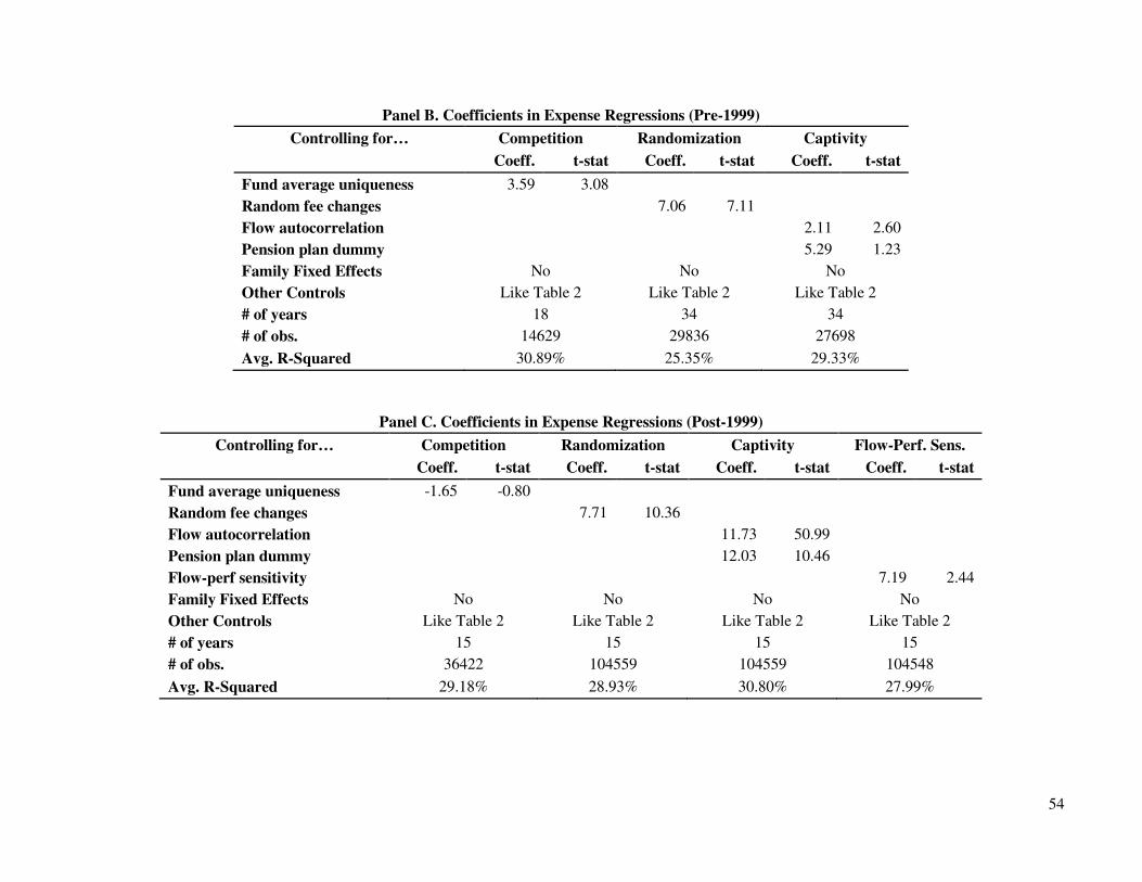
54
Panel B. Coefficients in Expense Regressions (Pre-1999)
Controlling for… Competition Randomization Captivity
Coeff. t-stat Coeff. t-stat Coeff. t-stat
Fund average uniqueness 3.59 3.08
Random fee changes 7.06 7.11
Flow autocorrelation 2.11 2.60
Pension plan dummy 5.29 1.23
Family Fixed Effects No No No
Other Controls Like Table 2 Like Table 2 Like Table 2
# of years 18 34 34
# of obs. 14629 29836 27698
Avg. R-Squared 30.89% 25.35% 29.33%
Panel C. Coefficients in Expense Regressions (Post-1999)
Controlling for… Competition Randomization Captivity Flow-Perf. Sens.
Coeff. t-stat Coeff. t-stat Coeff. t-stat Coeff. t-stat
Fund average uniqueness -1.65 -0.80
Random fee changes 7.71 10.36
Flow autocorrelation 11.73 50.99
Pension plan dummy 12.03 10.46
Flow-perf sensitivity 7.19 2.44
Family Fixed Effects No No No No
Other Controls Like Table 2 Like Table 2 Like Table 2 Like Table 2
# of years 15 15 15 15
# of obs. 36422 104559 104559 104548
Avg. R-Squared 29.18% 28.93% 30.80% 27.99%
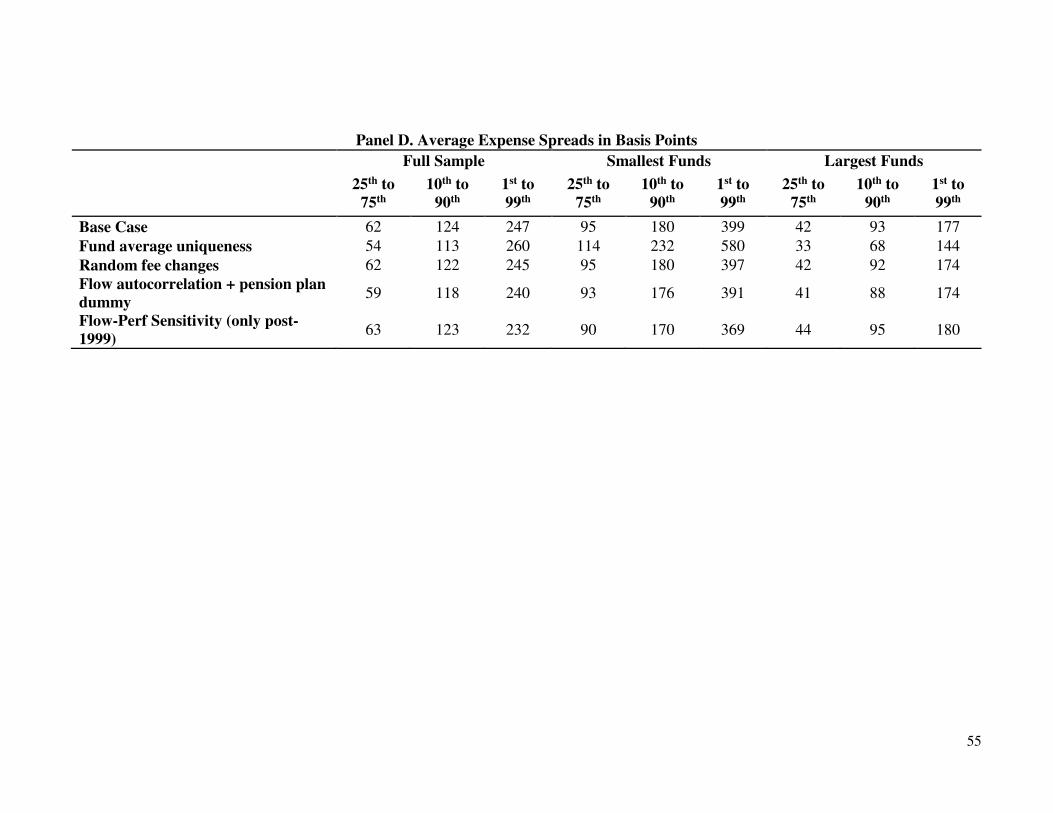
55
Panel D. Average Expense Spreads in Basis Points
Full Sample Smallest Funds Largest Funds
25th to
75th
10th to
90th
1st to
99th
25th to
75th
10th to
90th
1st to
99th
25th to
75th
10th to
90th
1st to
99th
Base Case 62 124 247 95 180 399 42 93 177
Fund average uniqueness 54 113 260 114 232 580 33 68 144
Random fee changes 62 122 245 95 180 397 42 92 174
Flow autocorrelation + pension plan
dummy 59 118 240 93 176 391 41 88 174
Flow-Perf Sensitivity (only post-
1999) 63 123 232 90 170 369 44 95 180

56
Table 8. US Household Participation, Average Fee Levels and Fee Dispersion
This table investigates the time-series relation between US household participation in the mutual fund industry and average fees or measures of
fee dispersion, respectively. Panel A reports summary statistics of the variables in levels and percentage changes. Panel B presents the regression
results in which all variables are included as percentage growth rates (i.e., relative changes). US Household participation is the percentage of
US household owning mutual funds. The data is obtained from the Investment Company Institute (ICI) Perspective Report (2014) and is
available starting in 1980. VW (EW) average fees are TNA-weighted (equally-weighted) averages of reported expense ratios. 90-10 reported
(residual) expense spread is the 90th percentile of reported (residual) expenses minus the 10th percentile of reported (residual) expense. The
percentiles of reported fees are derived from the empirical fee distribution of each yearly cross-section. Residual fees are derived from the
regressions reported in Table 2.
Panel A. Descriptive Statistics
Full Sample Largest Funds
Levels %-Changes Levels %-Changes
Mean SD Mean SD Mean SD Mean SD
US Household participation 32.51% 13.39% 7.17% 12.27%
VW Average Fees 0.79% 0.12% -0.05% 7.19% 0.74% 0.12% 1.05% 7.38%
EW Average Fees 1.26% 0.23% 0.98% 9.88% 0.94% 0.17% 1.01% 6.27%
90-10 Reported Expense Spread 1.47% 0.32% 1.72% 11.14% 1.06% 0.33% 3.59% 13.52%
90-10 Residual Expense Spread 1.24% 0.32% 2.39% 16.96% 0.84% 0.24% 3.67% 12.84%
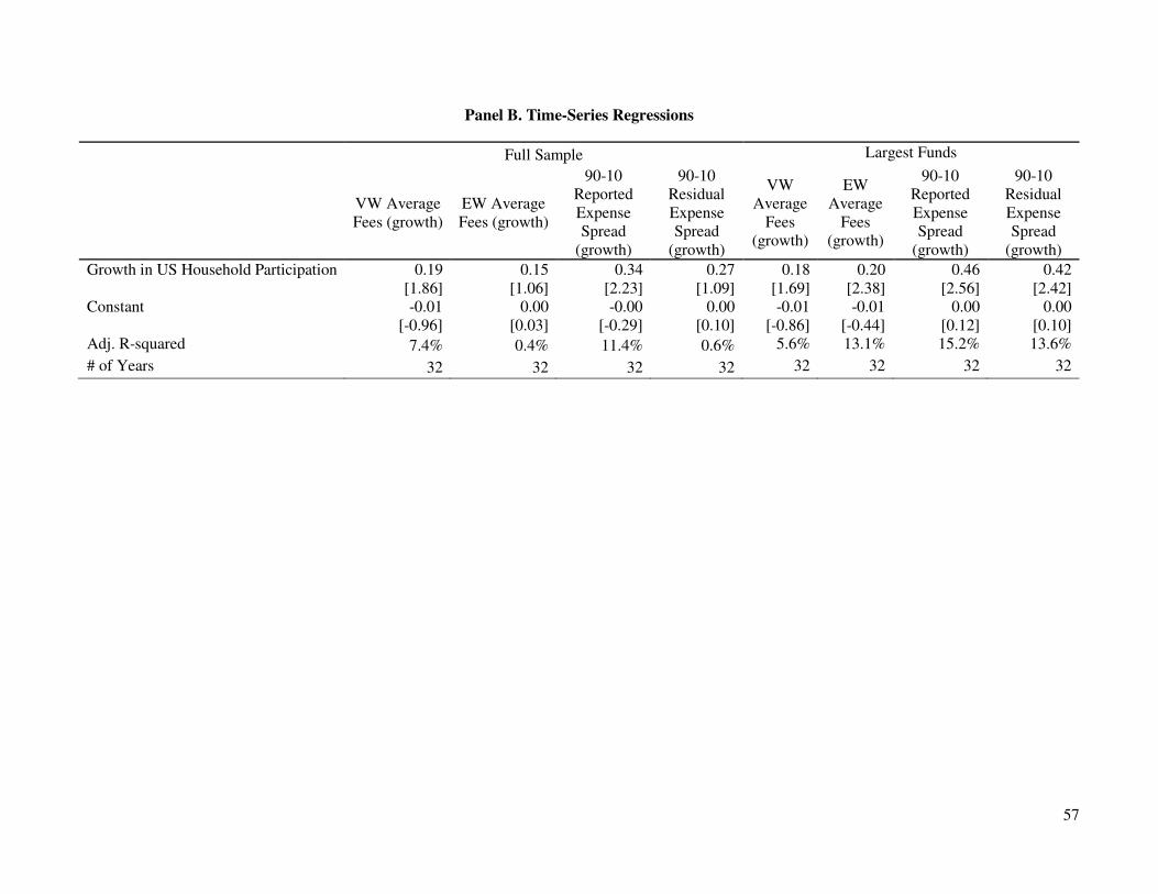
57
Panel B. Time-Series Regressions
Full Sample Largest Funds
VW Average
Fees (growth)
EW Average
Fees (growth)
90-10
Reported
Expense
Spread
(growth)
90-10
Residual
Expense
Spread
(growth)
VW
Average
Fees
(growth)
EW
Average
Fees
(growth)
90-10
Reported
Expense
Spread
(growth)
90-10
Residual
Expense
Spread
(growth)
Growth in US Household Participation 0.19
[1.86]
0.15
[1.06]
0.34
[2.23]
0.27
[1.09]
0.18
[1.69]
0.20
[2.38]
0.46
[2.56]
0.42
[2.42]
Constant -0.01
[-0.96]
0.00
[0.03]
-0.00
[-0.29]
0.00
[0.10]
-0.01
[-0.86]
-0.01
[-0.44]
0.00
[0.12]
0.00
[0.10]
Adj. R-squared 7.4% 0.4% 11.4% 0.6% 5.6% 13.1% 15.2% 13.6%
# of Years 32 32 32 32 32 32 32 32
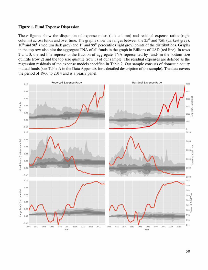
58
Figure 1. Fund Expense Dispersion
These figures show the dispersion of expense ratios (left column) and residual expense ratios (right
column) across funds and over time. The graphs show the ranges between the 25th and 75th (darkest grey),
10th and 90th (medium dark grey) and 1st and 99th percentile (light grey) points of the distributions. Graphs
in the top row also plot the aggregate TNA of all funds in the graph in Billions of USD (red line). In rows
2 and 3, the red line represents the fraction of aggregate TNA represented by funds in the bottom size
quintile (row 2) and the top size quintile (row 3) of our sample. The residual expenses are defined as the
regression residuals of the expense models specified in Table 2. Our sample consists of domestic equity
mutual funds (see Table A in the Data Appendix for a detailed description of the sample). The data covers
the period of 1966 to 2014 and is a yearly panel.
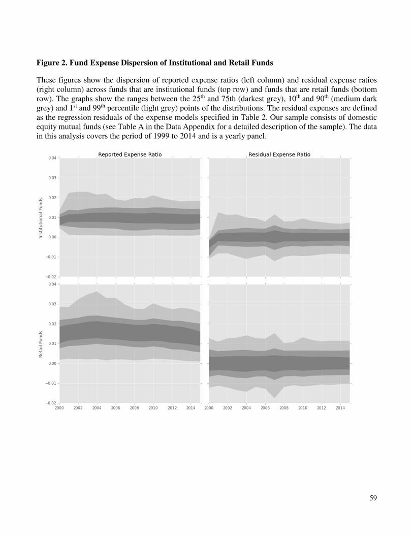
59
Figure 2. Fund Expense Dispersion of Institutional and Retail Funds
These figures show the dispersion of reported expense ratios (left column) and residual expense ratios
(right column) across funds that are institutional funds (top row) and funds that are retail funds (bottom
row). The graphs show the ranges between the 25th and 75th (darkest grey), 10th and 90th (medium dark
grey) and 1st and 99th percentile (light grey) points of the distributions. The residual expenses are defined
as the regression residuals of the expense models specified in Table 2. Our sample consists of domestic
equity mutual funds (see Table A in the Data Appendix for a detailed description of the sample). The data
in this analysis covers the period of 1999 to 2014 and is a yearly panel.
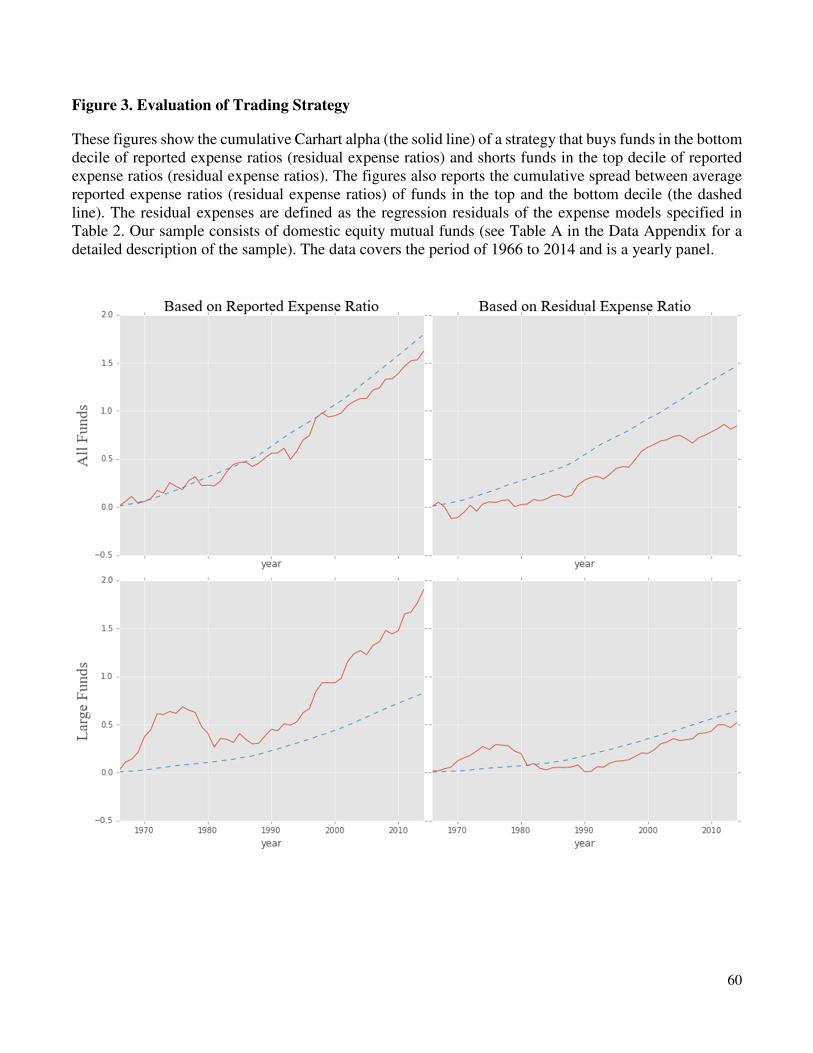
60
Figure 3. Evaluation of Trading Strategy
These figures show the cumulative Carhart alpha (the solid line) of a strategy that buys funds in the bottom
decile of reported expense ratios (residual expense ratios) and shorts funds in the top decile of reported
expense ratios (residual expense ratios). The figures also reports the cumulative spread between average
reported expense ratios (residual expense ratios) of funds in the top and the bottom decile (the dashed
line). The residual expenses are defined as the regression residuals of the expense models specified in
Table 2. Our sample consists of domestic equity mutual funds (see Table A in the Data Appendix for a
detailed description of the sample). The data covers the period of 1966 to 2014 and is a yearly panel.
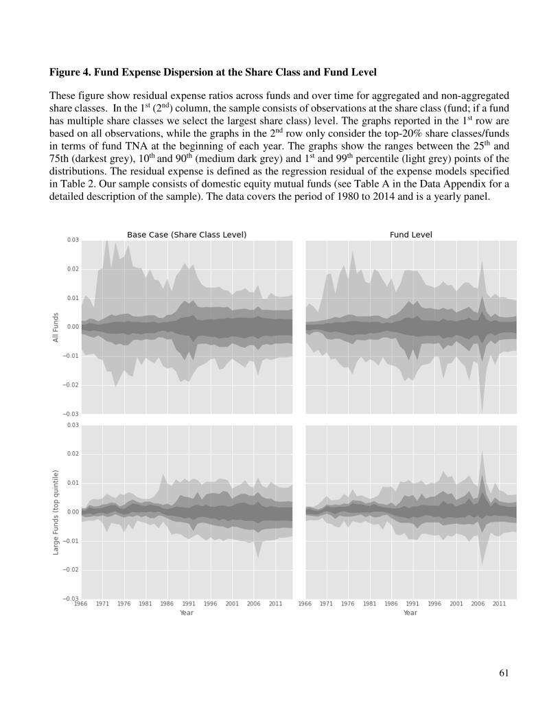
61
Figure 4. Fund Expense Dispersion at the Share Class and Fund Level
These figure show residual expense ratios across funds and over time for aggregated and non-aggregated
share classes. In the 1st (2nd) column, the sample consists of observations at the share class (fund; if a fund
has multiple share classes we select the largest share class) level. The graphs reported in the 1st row are
based on all observations, while the graphs in the 2nd row only consider the top-20% share classes/funds
in terms of fund TNA at the beginning of each year. The graphs show the ranges between the 25th and
75th (darkest grey), 10th and 90th (medium dark grey) and 1st and 99th percentile (light grey) points of the
distributions. The residual expense is defined as the regression residual of the expense models specified
in Table 2. Our sample consists of domestic equity mutual funds (see Table A in the Data Appendix for a
detailed description of the sample). The data covers the period of 1980 to 2014 and is a yearly panel.
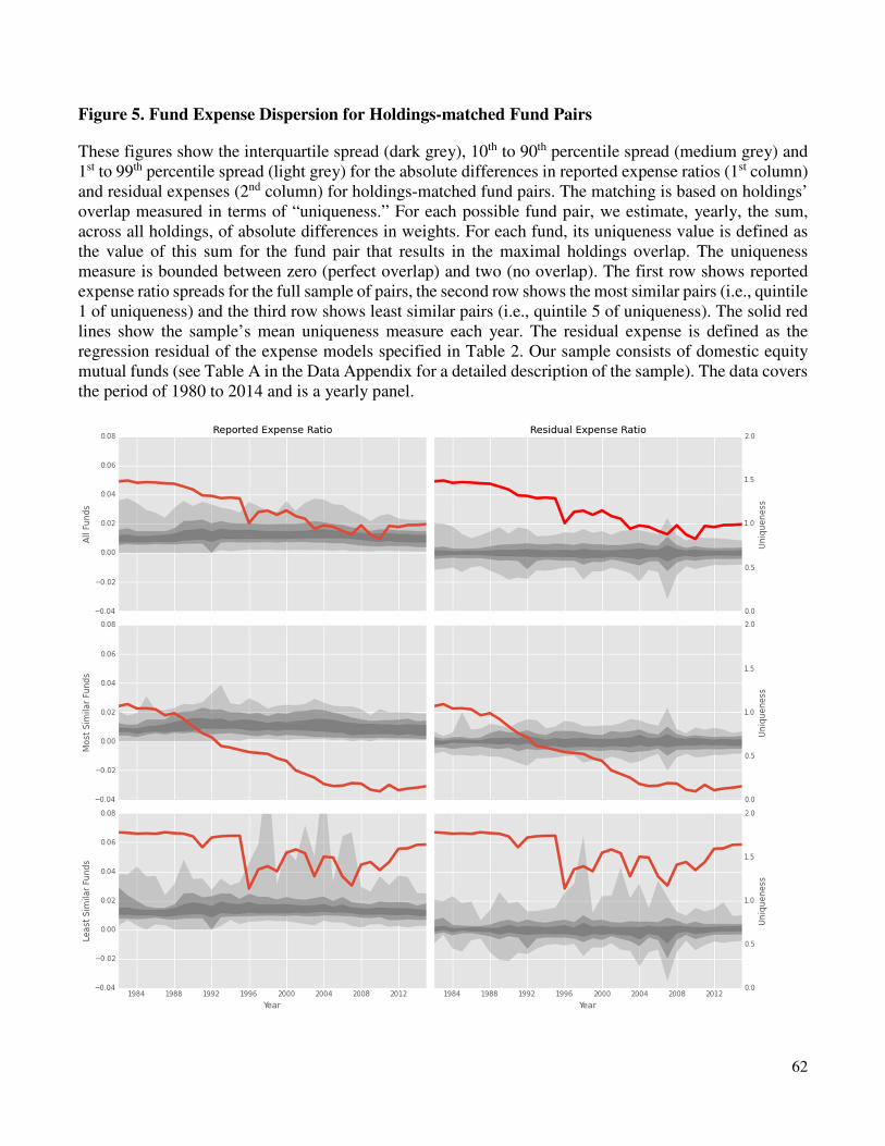
62
Figure 5. Fund Expense Dispersion for Holdings-matched Fund Pairs
These figures show the interquartile spread (dark grey), 10th to 90th percentile spread (medium grey) and
1st to 99th percentile spread (light grey) for the absolute differences in reported expense ratios (1st column)
and residual expenses (2nd column) for holdings-matched fund pairs. The matching is based on holdings’
overlap measured in terms of “uniqueness.” For each possible fund pair, we estimate, yearly, the sum,
across all holdings, of absolute differences in weights. For each fund, its uniqueness value is defined as
the value of this sum for the fund pair that results in the maximal holdings overlap. The uniqueness
measure is bounded between zero (perfect overlap) and two (no overlap). The first row shows reported
expense ratio spreads for the full sample of pairs, the second row shows the most similar pairs (i.e., quintile
1 of uniqueness) and the third row shows least similar pairs (i.e., quintile 5 of uniqueness). The solid red
lines show the sample’s mean uniqueness measure each year. The residual expense is defined as the
regression residual of the expense models specified in Table 2. Our sample consists of domestic equity
mutual funds (see Table A in the Data Appendix for a detailed description of the sample). The data covers
the period of 1980 to 2014 and is a yearly panel.
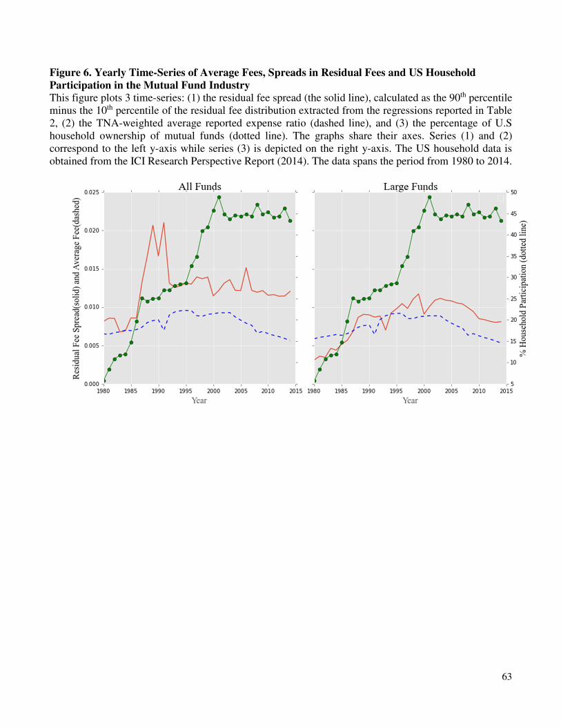
63
Figure 6. Yearly Time-Series of Average Fees, Spreads in Residual Fees and US Household
Participation in the Mutual Fund Industry This figure plots 3 time-series: (1) the residual fee spread (the solid line), calculated as the 90th percentile
minus the 10th percentile of the residual fee distribution extracted from the regressions reported in Table
2, (2) the TNA-weighted average reported expense ratio (dashed line), and (3) the percentage of U.S
household ownership of mutual funds (dotted line). The graphs share their axes. Series (1) and (2)
correspond to the left y-axis while series (3) is depicted on the right y-axis. The US household data is
obtained from the ICI Research Perspective Report (2014). The data spans the period from 1980 to 2014.