STUDYING SEEPAGE IN A BODY OF EARTH-FILL DAM BY

STUDYING SEEPAGE IN A BODY OF EARTH-FILL DAM BY

(ARTIFICIAL NEURAL NETWORKS) ANNs

A Dissertation Submitted to the Graduate School in Partial Fulfillment of the

Requirements for the Degree of

MASTER OF SCIENCE

Department: Civil Engineering Major: Water Resources Engineering

By Deniz ERSAYIN

January 2006 �zmir

ii

We approve the thesis of Deniz ERSAYIN

Date of Signature

........................................................ 05 January 2006

Prof. Dr. Gökmen TAYFUR Supervisor Department of Civil Engineering �zmir Institute of Technology

........................................................ 05 January 2006

Assist. Prof. Dr. �ebnem ELÇ� Department of Civil Engineering �zmir Institute of Technology

........................................................ 05 January 2006

Assoc. Prof. Dr. Sevinç ÖZKUL Department of Civil Engineering Dokuz Eylül University ........................................................ 05 January 2006 Prof. Dr. Gökmen TAYFUR Head of Department �zmir Institute of Technology

.................................................................. Assoc. Prof. Dr. Semahat ÖZDEM�R

Head of the Graduate School

iii

ACKNOWLEDGEMENT

I would like to express my sincere thanks to Prof. Dr. Gökmen Tayfur for his

guidance and valuable helps throughout the research. I also would like to thank Assist.

Prof. Dr. �ebnem �eker Elçi for her valuable helps and advises.

I would like to express my grateful thanks to my all family members Nur,

Kayhan, and Erdem Ersayın for their unlimited supports in all my life.

Special thanks go to Özden Sargın for his valuable helps and support.

Finally, I would like to express my grateful thanks to my colleagues.

iv

ABSTRACT

Dams are structures that are used especially for water storage, energy

production, and irrigation. Dams are mainly divided into four parts on the basis of the

type and materials of construction as gravity dams, buttress dams, arch dams, and

embankment dams. There are two types of embankment dams: earthfill dams and

rockfill dams.

In this study, seepage through an earthfill dam’s body is investigated using an

artificial neural network model. Seepage is investigated since seepage both in the dam’s

body and under the foundation adversely affects dam’s stability. This study specifically

investigated seepage in dam’s body. The seepage in the dam’s body follows a phreatic

line. In order to understand the degree of seepage, it is necessary to measure the level of

phreatic line. This measurement is called as piezometric measurement.

Piezometric data sets which are collected from Jeziorsko earthfill dam in Poland

were used for training and testing the developed ANN model. Jeziorsko dam is a non-

homogeneous earthfill dam built on the impervious foundation.

Artificial Neural Networks are one of the artificial intelligence related

technologies and have many properties. In this study the water levels on the upstream

and downstream sides of the dam were input variables and the water levels in the

piezometers were the target outputs in the artificial neural network model.

In the line of the purpose of this research, the locus of the seepage path in an

earthfill dam is estimated by artificial neural networks. MATLAB 6 neural network

toolbox is used for this study.

v

ÖZ

Barajlar, özellikle suyu biriktirmek, enerji üretmek ve sulama yapmak için

kullanılan yapılardır. Barajlar ba�lıca dört gruba ayrılır. Bunlar; A�ırlık barajları,

payandalı barajlar, kemer barajlar ve dolgu barajlardır. Dolgu barajlar ekonomiklikleri

açısından daha çok tercih edilir. Dolgu barajlar iki gruba ayrılır. Bunlar toprak dolgu

barajlar ve kaya dolgu barajlardır.

Bu çalı�mada, bir toprak dolgu baraj gövdesindeki sızma, yapay sinir a�ları

(YSA) metodu kullanılarak yapılan modelleme aracılı�ıyla incelenmi�tir. Sızmanın

incelenme amacı, sızmanın hem baraj gövdesinde hem de temelin altında do�rudan

baraj stabilitesine kar�ı bir tehdit olu�turmasıdır.Bu çalı�mada spesifik olarak baraj

gövdesindeki sızma incelenmi�tir. Baraj gövdesindeki sızma, freatik çizgi denilen bir

hattı takip eder. Sızmanın derecesini anlayabilmek için, freatik çizginin seviyesini

ölçmek gereklidir. Bu ölçüm piyezometrik ölçüm olarak adlandırılır.

Modellemede kullanılacak, piyezometrik ölçümlerin olu�turdu�u veri grubu,

Polonya’da bulunan Jeziorsko toprak dolgu barajından elde edilmi� olup, yapay sinir

a�ları modellemesinde e�itim ve sınama için kullanılmı�tır. Bu veri grubu,

piyezometrelerdeki su seviyeleriyle, baraj menba ve mansabındaki su seviyelerini

kapsamaktadır. Jeziorskobarajı, geçirimsiz zemin üzerine oturmu�, homojen olmayan

bir toprak dolgu barajdır.Piyezometrik ölçümler, Var�ova’da bulunan, meteoroloji ve su

yönetim enstitüsü baraj gözlem merkezince yapılmı�tır.

Yapay sinir a�ları yapay zeka ile ilgili teknolojilerden biridir ve birçok özelli�i

vardır.Yapay sinir a�ları, örneklerden ö�renir ve veriler arasında fonksiyonel bir ili�ki

yakalarlar. Bu çalı�mada barajın menba ve mansabına ait olan su seviyeleri, giri�

de�i�kenleri olarak kullanılmı�tır; piyezometrelerdeki su seviyeleri ise yapay sinir a�ları

modellemesinde hedef çıktı verisi olarak kullanılmı�tır.

Bu çalı�manın amacı, bir toprak dolgu barajdaki sızmanın geometrik yerini

yapay sinir a�ları metodunu kullanarak hesaplamaktır.

vi

TABLE OF CONTENTS

LIST OF FIGURES ....................................................................................................... viii

LIST OF TABLES............................................................................................................ x

CHAPTER 1. INTRODUCTION ................................................................................... 1

CHAPTER 2. DAMS....................................................................................................... 4

2.1. Main Functions of the Dams .................................................................. 4

2.2. The History of the dams ......................................................................... 5

2.3. The Types of Dams.............................................................................. 15

2.3.1. Gravity Dams ................................................................................. 16

2.3.2. Arch Dams ..................................................................................... 16

2.3.3. Buttress Dams ................................................................................ 17

2.3.4. Embankment Dams ........................................................................ 18

2.3.4.1. Earthfill Dams ....................................................................... 18

2.3.4.2. Rockfill Dams ....................................................................... 20

2.4. The Forces acting on dams................................................................... 21

2.4.1. Water Pressure ............................................................................... 21

2.4.2. Weight ............................................................................................ 21

2.4.3. Earthquakes .................................................................................... 22

2.4.4. Forces like ice, rain, waves ............................................................ 22

2.5. Seepage in earthfill dams and the importance of seepage in dam’s

body...................................................................................................... 22

2.6. Piezometric measurement of seepage in an earthfill dam’s body........ 23

CHAPTER 3. ARTIFICIAL NEURAL NETWORKS.................................................. 25

3.1. Historical Development of Artificial Neural Networks....................... 26

3.2. Fundamentals of Neural Networks ...................................................... 27

3.3. Artificial Neurons and the Basic Components of Artificial

Neurons ................................................................................................ 28

vii

3.4. Artificial Neural Networks and their Architecture ( Topology ) ......... 32

3.5. Learning Laws ..................................................................................... 33

3.6. Back-Propagation Algorithm ............................................................... 35

3.6.1. Background and Topology of the Back-Propogation

Algorithm....................................................................................... 35

CHAPTER 4. MODEL APPLICATION...................................................................... 39

CHAPTER 5. RESULTS AND DISCUSSION............................................................ 45

CHAPTER 6. CONCLUSIONS ................................................................................... 71

REFERENCES ............................................................................................................... 73

viii

LIST OF FIGURES

Figure Page

Figure 2.1. Main components of a dam ......................................................................... 4

Figure 2.2. Graphical representation of construction purposes of a dam ...................... 5

Figure 2.3. Keban Dam ................................................................................................ 16

Figure 2.4. Karakaya Dam ........................................................................................... 17

Figure 2.5. A buttress dam in the USA ........................................................................ 18

Figure 2.6. Anita Dam.................................................................................................. 19

Figure 2.7. Hasan U�urlu Dam .................................................................................... 20

Figure 3.1. A biological neuron and its components.................................................... 29

Figure 3.2. An artificial neuron and its structure ......................................................... 29

Figure 3.3. Linear transfer function ............................................................................. 30

Figure 3.4. Step transfer function................................................................................. 30

Figure 3.5. Gaussian transfer function ......................................................................... 31

Figure 3.6. Sigmoid transfer function .......................................................................... 31

Figure 3.7. Linearly separable two clusters.................................................................. 36

Figure 3.8. Structures of MLPs .................................................................................... 37

Figure 4.1. Example of seepage path through an earthfill dam.................................... 40

Figure 4.2. Seepage through a dam embankment with rock toe or gravel

blanket........................................................................................................ 40

Figure 4.3. Detail Cross-Section Sketch of the Jeziorsko Earthfill dam with

depicted soil layers..................................................................................... 41

Figure 5.1. Temporal Variations of the Water Level at Piezometers and in

upper and lower reservoirs......................................................................... 45

Figure 5.2. Comparison of measured versus ANNs model predicted data.

Training Stage............................................................................................ 46


Testing stage .............................................................................................. 47

Figure 5.4. Calculated and Measured Water Levels at piezometers.

Calibration Run.......................................................................................... 49

ix


Validation Run........................................................................................... 51


Training Stage ........................................................................................... 53


Testing Stage ............................................................................................. 54


Calibration Run.......................................................................................... 56


Validation Run........................................................................................... 58

Figure 5.10. Comparison of correlation coefficient, R2, with the results which

are obtained using different learning rates................................................. 60

Figure 5.11. Comparison of correlation coefficient, R2, with the results which

are obtained using different iteration numbers .......................................... 61


Training Stage............................................................................................ 63


Testing Stage ............................................................................................. 64


Calibration Run.......................................................................................... 66


Validation Run........................................................................................... 68

x

LIST OF TABLES

Table Page

Table 2.1. Tables about the embankment dams............................................................... 7

Table 2.2. Classification of the dams............................................................................. 21

Table 3.1. A brief history of neural Networks ............................................................... 27

Table 4.1. Schematic representation of the model design ............................................. 42

Table 5.1. Calculated error measures. Calibration Run ................................................. 52

Table 5.2. Calculated error measures. Validation Run .................................................. 52



Table 5.5. Results of R2 values with different topologies.............................................. 62



Table 5.8. Results of R2 values with different topologies.............................................. 70

1

CHAPTER 1

INTRODUCTION

A dam is an artificial barrier usually constructed across a stream channel to

capture water. Dams must have spillway systems to convey normal stream and flood

flows over, around, or through the dam. Spillways are commonly constructed of non-

erosive materials such as concrete. Dams should also have a drain or other water-

withdrawal facility for control the water level and to lower or drain the lake for normal

maintenance and emergency purposes. Dams are constructed especially for water

supply, flood control, irrigation, energy production, recreation, and fishing. Dams are

mainly divided into four parts on the basis of their structure types. These are gravity

dams, buttress dams, arch dams, and embankment dams. Embankment dams are more

preferable due to being more economical. Embankment dams are two types- Earthfill

dams and rockfill dams. This study is an investigation about earthfill dams, especially

about seepage through the earthfill dam’s body.

An earthfill dam is an embankment dam, constructed primarily of compacted

earth, either homogeneous or zoned, and containing more than 50% of earth. The

materials are usually excavated or quarried from nearby sites, preferably within the

reservoir basin. If the remaining materials consist of coarse particles, there is gradation

in fineness from the core to the coarse outer materials. According to the materials

located in the body of dam, there is a seepage through the dam’s body. Seepage can

occur under the dam foundation, too. In this research, seepage through the dam’s body

was investigated.

Seepage is very important, as seepage affects the stability of dam. Because of its

importance, the determination of the seepage through an earthdam has received a great

deal of attention. Of primary concern is the location of the surface seepage on the

downstream toe of the dam. There is seepage in the dam’s body following a phreatic

line. This seepage must be limited, and phreatic line is important in order to understand

the degree of seepage. If the surface seepage intersects the face of the dam, erosion may

result and possible failure of the dam. Thus, it is necessary to measure the level of

phreatic line and rockfills are used at the downstream toe or gravel blankets to intersect

the line of seepage before it reaches the downstream toe.

2

Up to now, seepage under the dam foundation is usually investigated. However,

in this research seepage through the earthfill dam’s body was investigated. An artificial

neural network (ANN) model was developed for simulating seepage through a non-

homogeneous porous body of an earthfill dam.The model was calibrated and verified

using the piezometer data collected on a section of Jeziorsko earthfill dam in Poland.

The water levels on the upstream and downstream sides of the dam were input variables

and the water levels in the piezometers were the target outputs in the artificial neural

network model. Jeziorsko dam is a non-homogeneous earthfill dam built on the

impervious foundation. Piezometric measurements were made by the Institute of

Meteorology and Water Management, Dams Monitoring Centre located in Warsaw.

Artificial Intelligence (AI) is the field of Computer Science that attempts to give

computers humanlike abilities. The human brain is the ultimate example of a neural

network. The human brain consists of a network of over a billion interconnected

neurons. Neurons are individual cells that can process small amounts of information and

then activate other neurons to continue the process. A computer can be used to simulate

a biological neural network. This computer simulated network is called an artificial

neural network (ANN). Artificial Neural Networks have many properties. They are non-

linear structures shown to be highly flexible function approximators for the cases,

especially where the data relationships are unknown. Artificial Neural Networks are

data-driven self-adaptive methods. They learn from examples and capture functional

relationships among the data. This modeling approach with the ability to learn from

experience is very useful since it is often easier to have data set; Furthermore, artificial

neural networks are particularly adapt at solving problems that cannot be expressed as a

series of steps. Artificial neural networks are useful for recognizing patterns,

classification into groups, series prediction and data mining. Artificial neural network

training methods fall into the categories of supervised, unsupervised, and various hybrid

approaches. The most common form of neural network that is used in applications is the

feedforward back-propagation neural network.

The purpose of this research is to estimate the locus of the seepage path in an

earthfill dam using artificial neural network. MATLAB 6 neural network toolbox is

used for this study. The ANN model was a feedforward three layer neural network

employing a sigmoid function as activator and a back-propagation algorithm for

network learning. The water levels on the upstream and downstream sides of the dam

were input variables and the water levels in the piezometers were the target outputs in

3

the artificial neural networks model. The water levels computed by the models

compared with the measured levels in the piezometers satisfactorily. The model results

also revealed that the artificial neural network (ANN) performed as good as did the site

observation and measured field data. In addition, sensitivity analysis was carried out

trying different scenarios.

4

CHAPTER 2

DAMS

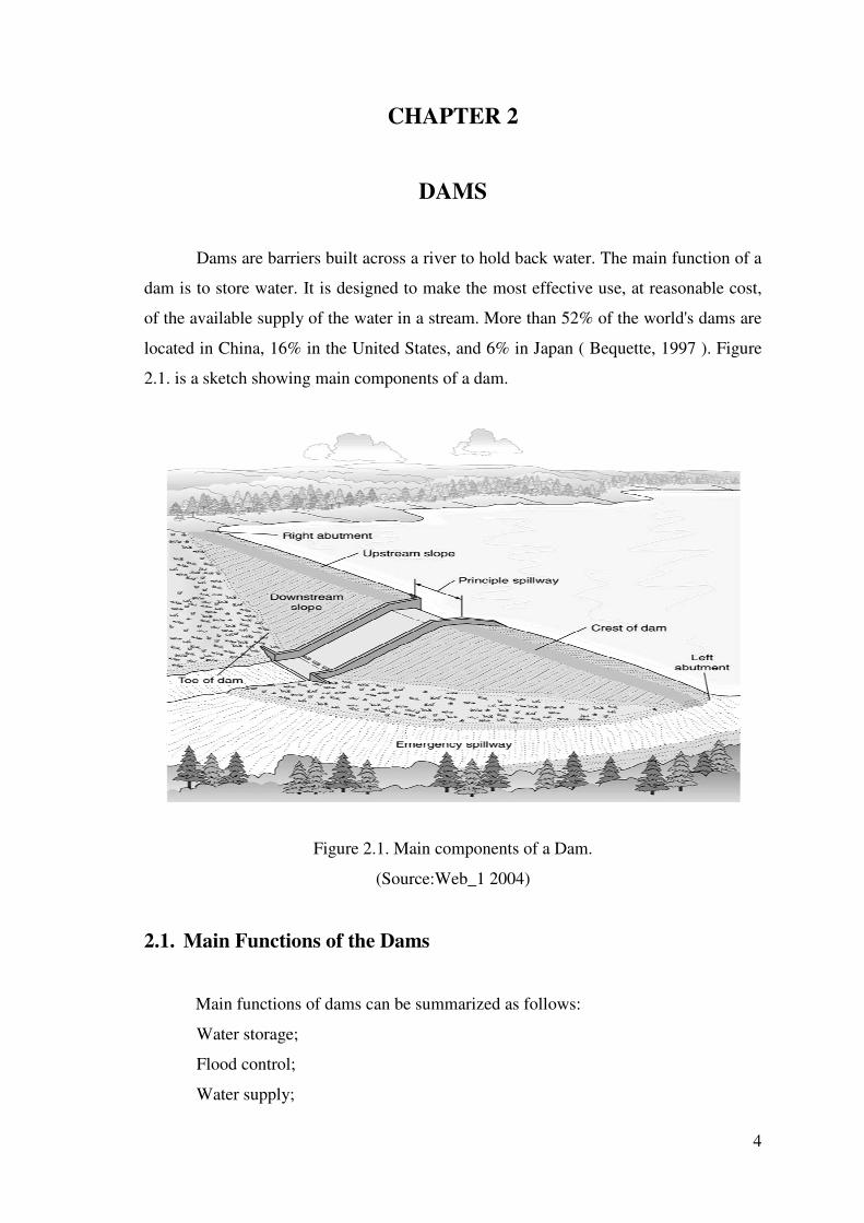
Dams are barriers built across a river to hold back water. The main function of a

dam is to store water. It is designed to make the most effective use, at reasonable cost,

of the available supply of the water in a stream. More than 52% of the world's dams are

located in China, 16% in the United States, and 6% in Japan ( Bequette, 1997 ). Figure

2.1. is a sketch showing main components of a dam.

�

Figure 2.1. Main components of a Dam.

(Source:Web_1 2004)

2.1. Main Functions of the Dams

Main functions of dams can be summarized as follows:

Water storage;

Flood control;

Water supply;

5

Power production;

Industrial water supply;

Emergency domestic water supply;

Irrigation; and

Recreation.

Figure 2.2. shows main construction purposes of a dam.

Figure 2.2. Graphical representation of construction purposes of a Dam.

(Source: Web_2 2004)

2.2. History of the Dams

The first dam for which there are reliable records was built in Jordan 5,000 years

ago to supply the city of Jawa with drinking water. During the reign of the Pharaoh

Amenemhet III, around 1800 B.C., the Egyptians constructed a reservoir with the

amazing storage capacity of 275 million [m.sup.3] in Al Fayyum Valley, some 90 km

southwest of Cairo. A large dam was built by an Arabian king called Lokman about

1700 B.C.; the flood caused by its collapse is recorded in Arabian history. Thousands of

dams have been built in India from the earliest days to the present time. The oldest

existing dams in Europe are the Almanza and Alicante dams in Spain; they were built

some time before 1586. In time, materials and methods of construction have improved,

making possible the erection of large dams such as the Nurek Dam which is being

6

constructed on the Vaksh River near the border of Afghanistan. This dam is designed

1017 ft

( 333 m ) high, of earth and rock fill. The failure of dam may cause serious loss of life

and property; consequently, the design and maintenance of dams are commonly under

government surveillance. In the United States over 30000 dams are under the control of

state authorities(Grolier Incorporated, 1970); (Güney, 2002); (Beuqette, 1997).

The General Directorate of State Hydraulic Works (DSI in Turkish acronym)

with a legal entity and supplementary budget is the primary executive state agency of

Turkey for Nation overall water resources planning, managing, execution, and

operation. The main objective of DSI is to develop all water and land resources in

Turkey. It aims at all the wisest use of the principal natural resources. DSI was

established by Law 6200 in December 18, 1953 as legal entity and brought under the

aegis of the Ministry of Energy and Natural Resources. It is charged with "single and

multiple utilization of surface and groundwaters and prevention of soil erosion and

flood damages". For that reason, DSI is empowered to plan, design, construct, and

operate dams, hydroelectric power plants, domestic water, and irrigation schemes. DSI's

purpose "to develop water and land resources in Turkey" covers a wide range of

interrelated functions. These include irrigation, hydroelectric power generation;

domestic and industrial water supplies for large cities; recreation and research on water-

related planning, design, and construction materials. Projects, master plan, and

feasibility reports are prepared for the development of water resources. In this respect,

required main data are collected by DSI from the river basin surveys which are related

with flow and meteorological, soil classification, agricultural economy, erosion, maps,

geological conditions etc. issues ( Web_3, 2004). Table 2.1 shows main embankment

dams especially earthfill dams in Turkey, with their construction purposes and

capacities.

7

Table 2.1. Tables about the embankment dams at (a), (b), (c), (d), (e), (f), (g), (h), (i),

(j), (k), (l), (m), (n), (o), (p), (q). These dams are constructed by DSI. Tables

are given according to the chronological construction year.

(a) GÖLBA�I DAM

Location Bursa

River Aksu

Purpose Irrigation, Flood control

Construction (starting and completion) year 1933-1938

Embankment type Earthfill

Dam volume 320 000 m3

Height (from river bed) 10.70 m

Reservoir volume at normal water surface elevation 12.75 hm3

Reservoir area at normal water surface elevation 1.74 km2

Irrigation Area 2 100 ha

(b)DEM�RKÖPRÜ DAM

Location Manisa

River Gediz


Energy

Construction (starting and completion) year 1954 - 1960


Dam volume 4 300 000 m3


Reservoir volume at normal water surface elevation 1 320.00 hm3



Capacity 69 MW

Annual generation 193 GWh

(Cont. on next page)

8

Table 2.1.(cont.)

(c) KES�KKÖPRÜ DAM

Location Ankara

River Kızılırmak

Purpose Irrigation, Energy


Embankment type Earthfill-Rockfill






Capacity 76 MW

Annual generation 250 GWh

(d) DAMSA DAM

Location Nevsehir

River Damsa

Purpose Irrigation

Construction (starting and completion) year 1965 -1971








9

Table 2.1.(cont.)

(e) ATIKH�SAR DAM

Location Çanakkale

River Sarıçay









(f) KORKUTEL� DAM

Location Antalya

River Korkuteli



Embankment type Earthfill+Rockfill







10

Table 2.1.(cont.)

(g) AF�AR DAM

Location Manisa

River Ala�ehir









(h) A�CASAR DAM

Location Kayseri

River Yahyalı

Purpose Irrigation




Height (from river bed) 25,00 m

Reservoir volume at normal water surface elevation 66,06 hm3

Reservoir area at normal water surface elevation 4,17 km2

Irrigation Area 15500 ha


11

Table 2.1.(cont.)

(i) KAYABO�AZI DAM

Location Kütahya

River Koca

Purpose Irrigation, Flood conrtol


Embankment type Earthfill+Rockfill






(j) KOVALI DAM

Location Kayseri

River Dündar

Purpose Irrigation









12

Table 2.1.(cont.)

(k) UZUNLU DAM

Location Yozgat

River Kozanözü









(l) �K�ZCETEPELER DAM

Location Balıkesir

River Kocadere

Purpose Irrigation, Domestic and

industrial water supply

Construction (starting and completion) year 1986 – 1990







Annual domestic water 72 hm3


13

Table 2.1.(cont.)

(m) KRALKIZI DAM

Location Batman

River Dicle

Purpose Energy


Embankment type Earthfill + Rockfill



Reservoir volume at normal water surface elevation 1 919.00 hm3


Irrigation Area 90 MW

Annual domestic water 146 GWh

(n) ÇAMLIGÖZE DAM

Location Sivas

River Kelkit

Purpose Energy, Flood control


Embankment type Earthfill+ Rockfill





Irrigation Area 33 MW

Annual domestic water 88 GWh


14

Table 2.1.(cont.)

(o) KARAOVA DAM

Location Kır�ehir

River Manahozu

Purpose Irrigation








(p) ERZ�NCAN DAM

Location Erzincan

River Gönye

Purpose Irrigation









15

Table 2.1.(cont.)

(q) GÖKPINAR DAM

Location Denizli

River Gökpınar

Purpose Irrigation+domestic water

supply








2.3. The Types of Dams

The basic types of the dams are classified on the basis of the structure type and

materials of construction. The dams which are classified on the basis of the structure

type are gravity dams, arch dams, buttress dams and embankment dams. Embankment

dams can be divided into two types as embankment earthfill dams and embankment

rockfill dams. The gravity, arch and buttress dams are usually constructed of concrete.

Dams that are classified on the basis of materials of construction are masonry dams,

filling dams, both masonry and filling dams, and framed dams. Masonry dams can be

divided into four parts as stone and brick dams, concrete dams, reinforced concrete

dams, and prestressed concrete dams. Filling dams can be divided into two types as

earthfill dams and rockfill dams. Lastly, framed dams can be divided into two parts as

steel dams and timber dams. Dams can also be classified according to usage purposes.

These are drinking water dams, industrial water dams, irrigation water dams,

hydroelectric power dams, and flood control dams. The most common type of dam is

embankment earthfill dams. The following summarize structure types of dams.

16

2.3.1. Gravity Dams

A gravity dam depends on its own weight for stability and is usually straight in

plan although sometimes slightly curved. It looks like a retaining wall, set across a river.

Keban dam on the Fırat river (Figure 2.3.) is an example of a gravity dam in Turkey.

Figure 2.3. Keban Dam.

(Source:Web_4 2005)

2.3.2. Arch Dams

Arch dams transmit most of the horizontal thrust of the water behind them to the

abutments by arch action and may have comparable thinner cross-sections than gravity

dams. Arch dams can be used only in narrow canyons where the walls are capable of

withstanding the thrust produced by the arch action. Karakaya dam on the Fırat river

(Figure 2.4.) and Oymapınar dam on the Manavgat river are examples of arch dams in

Turkey.

17

Figure 2.4. Karakaya Dam.


2.3.3. Buttress Dams

Buttress dams are dams in which the face is held up by a series of supports.

Buttress dams can take many forms. The face may be flat or curved. A buttress dam is

supported by a series of buttress walls, set at right angles to the dam on the downstream

side. There are several types of buttress dams, the most important ones are flat-slab and

multiple-arch buttress dams. Flat- slab and buttress dams are particularly adapted to

wide valleys where a long dam is required and foundation materials are of inferior

strength. The multiple-arch dam is more rigid than the flat-slab type and consequently

requires a better foundation. Elmalı dam on the Göksu river is an example of a buttress

dam in Turkey. Figure 2.5. shows a buttress dam.

18

Figure 2.5. A buttress dam in the USA.


2.3.4. Embankment Dams

Embankment dams can be divided into two types as earthfill dams and rockfill

dams.

2.3.4.1. Earthfill Dams

An earthfill dam is made up partly or entirely of pervious material which consists of

fine particles usually clay, or a mixture of clay and silt or a mixture of clay, silt and gravel.

They are principally constructed from available excavation material. The dam is built up

with rather flat slopes. Fine, impervious material of an earthfill dam occupies a relatively

small part of the structure, it is known as the core. The core is located either in a central

position or in a sloping position upstream of the center. If the remaining materials consist of

coarse particles, there is a gradation in fineness from the core to the coarse outer materials.

Some earth dams have a large proportion of rock in the outer zones for the purpose of

stability. In a later section in this thesis, the importance of the stability in an earthfill dam

especially in the dam’s body, will be given in more detail. Most new earthfill dams are roll

fill type dams, which can be further classified as homogenous, zoned, or diaphragm (U.S.

Bureau of Reclamation, 1987). Homogenous earthfill dams are composed of only one kind

of material, besides the slope protection material. The material used must be impervious

19

enough to provide an adequate water barrier and the slope must be relatively flat for

stability. It is more common today to build modified homogeneous sections in which

pervious materials are placed to control steeper slopes. When pervious material is used in

order to drain the material three methods are used. Rockfill toe, horizontal drainage blanket,

inclined filter drain with a horizontal drainage blanket. Pipe drains are also used for

drainage on small dams in conjunction with a horizontal drainage blanket or a pervious

zone. For diaphragm-type earthfill dams, the embankment is constructed of pervious

materials( sand, gravel, or rock ). A thin diaphragm of impermeable material is used to form

a water barrier. The diaphragm may vary from a blanket on the upstream face to a central

vertical core. Diaphragms may consist of earth, portland cement concrete, bituminous

concrete, or other materials. In addition, the diaphragm must be tied into bedrock or a very

impermeable material if excessive underseepage is to be avoided. Zoned embankment-type

earthfill dams have a central impervious core that is flanked by a zone of materials

considerably more pervious, called shells. These shells enclose, support, and protect the

impervious core (Linsley and Franzini, 1964). Demirköprü dam on the Gediz river and

Aslanta� dam on the Ceyhan river are examples of earthfill dams in Turkey.

Figure 2.6. Anita Dam.


Figure 2.6. shows the Warm Springs earthfill dam in the USA.

20

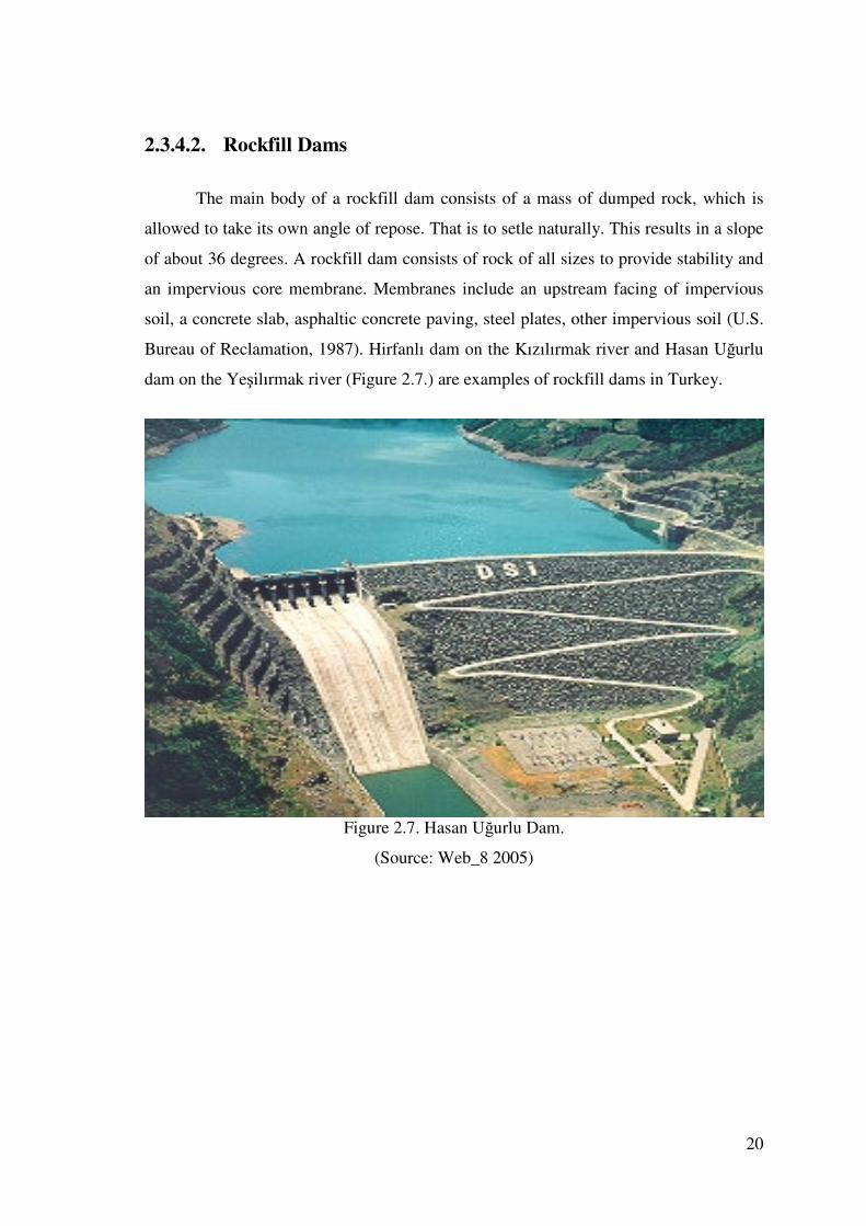
2.3.4.2. Rockfill Dams

The main body of a rockfill dam consists of a mass of dumped rock, which is

allowed to take its own angle of repose. That is to setle naturally. This results in a slope

of about 36 degrees. A rockfill dam consists of rock of all sizes to provide stability and

an impervious core membrane. Membranes include an upstream facing of impervious

soil, a concrete slab, asphaltic concrete paving, steel plates, other impervious soil (U.S.

Bureau of Reclamation, 1987). Hirfanlı dam on the Kızılırmak river and Hasan U�urlu

dam on the Ye�ilırmak river (Figure 2.7.) are examples of rockfill dams in Turkey.

Figure 2.7. Hasan U�urlu Dam.


21

Table 2.2. Classification of the dams.

On the basis of the

structure

On the basis of the

materials of construction

According to usage

purpose

a. Gravity Dams

b Arch Dams

c. Buttress Dams

d Embankment Dams

- Earthfill Dams

- Rockfill Dams

a. Masonry Dams

-Stone and Brick Dams

-Concrete Dams

-Reinforced Concrete Dams

-Prestressed Concrete Dams

b. Filling Dams

-Earthfill Dams

-Rockfill Dams

c. Masonry and Filling Dams

d. Framed Dams

-Steel Dams

-Timber Dams

a. Dams for drinking water

b. Dams for Industrial water

c. Dams for irrigation

d. Dams for flood control

e.Dams for Hydroelectric

Power

f. Cofferdams

Table 2.2. shows the classification of dams.

2.4. The Forces acting on dams

Main forces which are acting on dams can be summarized as follows.

2.4.1. Water Pressure

Water pressure is the most obvious force that is exerted by the water that presses

upon the upstream face of structure. In designing a dam, when silt builds up against the

lower part of the dam, it acts as a liquid that is denser than water. Engineers must take

this factor also in dam design.

2.4.2. Weight

The weight of the dam itself is another force that acts on dam structures. This

factor is important mainly in the case of gravity dams and very high arc dams. Concrete

22

can withstand pressure such as the vertical downward pressure. To reduce the stress on

weak foundations, a limit must be set to the height of the dam, and the upstream face

must be sloped so as to spread the load. The weight of the water pressing down on the

slope will act as a satabilizing factor.

2.4.3. Earthquakes

Earthquakes may exert considerable pressure on dams. The action is like that of

pulling a rug from under a person who is standing on it. The horizontal force exerted by

an earthquake may be equal to as much as a tenth of the weight of the dam; hence earthquake forces are usually taken into account in the design stage of a dam.

2.4.4. Forces like Ice, Rain, Waves

Ice is another factor that must be considered. In cold climates a thick sheet of ice

may form on the reservoir surface. Such a sheet of ice may be warmed by the sun. The tendency to expand may then cause a huge force near the top of the dam. Hence this part of the structure must be made thick enough to withstand the pressure. Seasonal and daily changes in temperature may cause internal stresses in dams . These changes must

be carefully analyzed. Waves striking against the face of a gravity or arch dam have

little effect on the stability of the structure. In the case of an earthfill dam, however, the

waves would soon erode the surface material if it were not protected by a facing of

heavy rock laid on a bed of gravel. Such rock is known as riprap. The erosive forces of

nature – winds, rain, running water etc. – are always at work. To be able to keep these

forces in check, periodic maintenance work is required on all dams.

2.5. Seepage in Earthfill Dams and the Importance of Seepage in

Dam’s Body

An earthfill dam’s body prevents the flow of water from dam’s back to

downstream. However, with the most impermeable materials used in the dam’s body,

some amount of water seeps into dam’s body and goes out from downstream of body

slope until it meets an impermeable barrier. So if the water level at the upstream side is

23

rapidly lowered, the water-soaked material may become unstable. This has to be

considered in the design of earthfill dams. Earthfill dams are usually designed pervious,

and some seepage flow through the dam body must be expected.

Seepage flow which occurs in the earthfill dam’s body has a top surface. This

surface is called as phreatic line or zero pressure curve. However the upper zone of

phreatic line can be wet or saturated because of capillarity. There is a pore water

pressure under the phreatic line. According to the� analysises, value of pore water

pressure depends on the type tightness degree, humidity, and impermeability of soil, and

load on soil etc. Pore water pressure decreases the shearing resistance of earth mass. If

the rate of pore water pressure drop resulting from seepage exceeds the resistance of a

soil particle to motion, that particle will tend to move . This results in piping, the

removal of the finer particles from the dam’ s body. Piping usually occurs near the

downstream toe of a dam when seepage is excessive (Linsley and Franzini, 1964).

According to these reasons for stability of dam the level of seepage flow especially

phreatic line must be limited. In this thesis, there are measurement results for

determination of seepage flow using piezometers, in this thesis in a later section there

are model results which are obtained according to these piezometric measurement

results.

In addition, seepage in the dam’s body is important due to two reasons. First one

is that, phreatic line cuts downstream slab. The higher cutting of the dam slab because

of phreatic line is the more dangereous condition for the slab, because the soil under

that point will be saturated, when the soil saturation increases, pore water pressure

increases too and due to the quantity of saturation, collapse probability increases. That

makes the body of dam unstable. Second reason is maximum reservoir position that

contains the body’s maximum saturation degree is the most critical condition for the

downstream slab’s stability after the construction. The most critical condition for

upstream slab’s stability is the sudden drop in the water level in the reservoir. That

makes the body of dam unstable.

2.6. Piezometric Measurement of Seepage in an Earthfill dam’ s Body

Seepage path in an earthfill dam can be monitored through piezometric

measurements. Piezometer is a device for a measurement of static pressure. Measuring

24

the static pressure in a flowing fluid requires that the measuring device fits the

streamlines as closely as possible. This is required so that no disturbance in the flow

will occur. For straight reaches of pipe conduit, the static pressure is usually measured

by using a piezometer. Measuring the static pressure in a flow field requires the use of a

static tube. For this device, the pressure is transmitted to a gauge or a manometer

through piezometric hole that are evenly spaced around the circumference of the tube.

The device must be perfectly aligned with the flow (Mays, 2001).

25

CHAPTER 3

ARTIFICIAL NEURAL NETWORKS

Artificial neural networks are mathematical modeling tools and computing

systems that are especially helpful in the field of prediction and forecasting in complex

settings. (Hamed et al.,2003). These computing systems are made up of a number of

simple and highly interconnected processing elements that process information by their

dynamic state response to external inputs (Caudill M.,1987). Mathematically, an

artificial neural network can be treated as a universal approximator which has an ability

to learn from examples without the need of explicit physics (ASCE Task Committee,

2000a, b). It is well known that the artificial neural network can be envisaged as a non-

linear black box model. That is given an input it produces an output, without revealing

the physics of the process (Rajurkar et al., 2003). ANNs have been recently employed

for the solution of many hydrologic, hydraulic and water resources problems ranging

from rainfall and runoff (Rajurkar et al. 2002) to sediment transport (Tayfur, 2002) to

dispersion (Tayfur and Singh, 2005).

Artificial neural networks are first developed in the simplest form by Widrow

and Hoff in the beginning of 1960’s which consist of two layers, input layer and output

node but only the output node has an activation function, which is a linear function and

it can only solve linearly separable problems. This simple architecture named

ADALINE (Adaptive Linear Neuron) Neural Networks. After ADALINE NN, new

architectures are developed like Multi Layer Perceptrons (MLP). In Multi Layer

Perceptrons some new activation functions are utilized like sigmoid or Gaussian

activation functions. Artificial intelligent methods are divided into three main categories

as supervised, unsupervised and reinforcement algorithms. MLPs are the most popular

and widely used supervised algorithms. Supervised algorithms need input-output pairs.

With these pairs, through the error propagation, network approximates a function. Apart

from supervised algorithms in unsupervised algorithm there is no error to back

propagate and there is no target to reach, instead, this type of algorithms only works on

input pairs and tries to arrange inputs according to pre-specified rules. Reinforcement

learning (RL) attempts to learn from its past experience and it is expected that after each

26

trial it is going to respond more rationally. In this research Backpropagation Neural

Network is used as MLP.

3.1. Historical Development of Artificial Neural Networks

The history of neural network development has been eventful, and exciting. The

history of neural networks shows the interplay among biological experimentation,

modeling, and computer simulation / hardware implementation. Thus, this field is

strongly interdisciplinary. Back in the 1940’s, first studies about neural networks began.

Warren McCulloch and Walter Pitts designed what are generally regarded as the first

neural networks (McCulloch & Pitts, 1943).

At the end of 1940’s, Donald Hebb, a psychologist at McGill University,

designed the first learning law for artificial neural networks (Hebb, 1949). He thougt

that if two neurons were active, then the strength of the connection between them

should be increased. This idea is closely related to the correlation matrix learning

developed by Kohonen (1972) and Anderson (1972) among others.

Frank Rosenblatt (1958, 1959, 1962) introduced and developed a large class of

artificial neural networks called perceptrons, together with several other researchers

(Block, 1962; Minsky & Papert, 1988). The most typical perceptron consisted of an

input layer connected by paths with fixed weights to associator neurons. In the

beginning of 1960’s, Bernard Widrow and his student, Marcian Ted Hoff (Widrow &

Hoff, 1960) developed a learning rule that is closely related to the perceptron learning

rule. The Widrow – Hoff learning rule for a single – layer network is a precursor of the

backpropagation rule for multilayer nets. Despite Minsky and Papert’s demonstration of

the limitations of perceptrons ( i.e.,single – layer nets ), research on neural networks

continued. In 1970’s, the early work of Teuvo Kohonen (1972), of Helsinki University

of Technology, dealt with associative memory neural nets.His more recent work

(Kohonen, 1982) has been the development of self – organizing feature maps. James

Anderson, of Brown University, also started his research in neural Networks with

associative memory nets (Anderson, 1968, 1972). In 1980’s, Gail Carpenter has

developed a theory of self – organizing neural networks called adaptive resonance

theory (Carpenter & Grossberg, 1985, 1987a, 1987b, 1990). Nobel prize winner John

Hopfield has developed a number of neural networks based on fixed weights and

27

adaptive activations together with a researcher, David Tank ( Hopfield & Tank, 1985,

1986 ). In 1980’s, Kunihiko Fukushima and his colleagues have also developed a series

of specialized neural nets for character recognition (Fukushima et al., 1983).

Table 3.1 shows a brief summary about the development of the artificial neural

networks.

Table 3.1. A brief history of neural networks (Nelson & Illingworth, 1991)

Conception 1890 James, Psychology ( Briefer Course )

Gestation 1936

1943

1949

Turing uses brain as computing paradigm

McCulloch & Pitts paper on neurons

Hebb, The Organization of Behaviour

Birth 1956 Darmouth Summer Research Project

Early

Infancy

Late 50’s,

60’s

Research efforts expand

Stunted

Growth

1969 Some research continues

Minsky & Papert ’ s critique, Perceptrons

Late

Infancy

1982 Hopfield at National Academy of Sciences

Present Late 80’s

to now

Interest explodes with conferences, simulations,

new companies, government funded research .

3.2. Fundamentals of Neural Networks

Neural networks are one of the few Artificial Intelligence – related technologies

that have a mathematical foundation. An artificial neural network is a flexible

mathematical structure which motivates from the operation of human nervous system. It

has many advantages and treats the arbitrary complex non – linear relationship between

the input and the output of any system (Rajurkar et al., 2003). Artificial neural networks

can be considered as non – linear function approximating tools (i.e.,linear combinations

of non – linear basis functions) having an ability to learn from examples, where the

28

parameters of the networks should be found by applying optimisation methods. The

optimisation is done with respect to the approximation error measure.

Neural networks are noted for mathematical basis, parallelism, distributed

associative memory, fault tolerance, adaptability, pattern recognition, intuition, and

statistical pattern recognition (Nelson & Illingworth, 1991). Neural networks are

particularly adept at solving problems that can not be expressed as a series of steps and

useful for recognizing patterns, classification into groups, series prediction, and data

mining.

Artificial Neural Networks can be divided particularly in two parts.

1) Architecture ( it defines the structure of the network )

2) Neurodynamics ( it includes properties as to how the network learns, recalls,

associates, and continously compares new information with existing knowledge.)

3.3. Artificial Neuron and the Basic Components of Artificial Neuron

Artificial neural networks are inspired by the learning processes that take place

in biological systems. To understand what is placed behind this inspiration, biological

neurons will be briefly discussed. Artificial neural Networks are made up of individual

models of the biological neuron (Figure 3.1.) that are connected together to form a

network. The neuron models used are much simplified versions of the actions of a real

neuron (Page et al., 1993). The human brain is very complex capable of thinking,

remembering, and solving. Fundamental unit of the brain’s nervous system is “neuron”.

This “neuron” is a simple processing element that receives and combines signals from

other neurons through input paths called “dendrites”. An artificial neuron (Figure 3.2.)

is a model whose components have direct analogies to components of biological neuron.

Due to two main reasons, artificial neural network is like human brain:

1) It stores knowledge through synaptic weights.

2) It learns from experiments and / or experience.

The most commonly used neuron model is based on the model proposed by

McCulloch and Pitts in 1943.

29

Biological Neuron

Figure 3.1. A biological neuron and its components.

Artificial Neuron

Figure 3.2. An artificial neuron and its structure.

An artificial neuron receives input, process it and then produce an output. It can

be called a processing element. It consists of mainly five parts.

1) Inputs and Outputs

There are many inputs (stimulation levels) to a neuron, there should be many

input signals to processing element. There may be many inputs to the neuron, but there

is only one output from the neuron. Just as real neurons are affected by things other than

inputs, some networks provide a mechanism for other influences. Sometimes this extra

input called a bias term (Nelson and Illingworth, 1994). There is bias node in the input

and hidden layers but not in the output layer. This one output is disributed by the

synaptic weights to each neuron in the next layer .

2) Weighting Factors

30

Each input will be given a relative weighting, which will affect the impact of

that input. Weights are adaptive coefficients within the network that determine the

intensity of the input signal (Nelson and Illingworth, 1994). The product of the inputs

and synaptic weights obtains every information carried to neuron ( i.e. ��W

�J ). In a

way each input is weighted before reaching the neuron .

3) Transfer ( Activation ) Functions

Transfer functions are functions that transform the net input to a neuron into its

activation. Also they are known as a transfer, or output function (Fausett, 1994). They

are usually non-linear. If the problem is non-linear, then non-linear is employed.

Commonly used non-linear functions are as follows:

• Linear Function

Figure 3.3. Linear transfer function.

The linear transfer function calculates (Figure 3.3.) the neuron’s output by

simple equation, where α is a constant.

a(n) = α x (3.1)

This neuron can be trained to find a linear approximation to a nonlinear function.

• Step ( Hard Limiter) Function

Figure 3.4. Step transfer function.

31

The hard limiter transfer function (Figure 3.4.) forces a neuron to output a β if

its net input reaches a threshold, otherwise it outputs α. This allows a neuron to make a

decision or classification (Tsoukalas and Uhrig, 1997). It can say yes or no. This kind of

neuron is often trained with the perceptron learning rule, and generally parameters are

chosen as β = 1 and α = 0 or 1 in the literature.

• Ramping or Rampage Function

For inputs less than -1 ramping function produces -1. For inputs in the range -1 to

+1 it simply returns to the linear function. For inputs greater than +1 it produces +1, but

this function is not a continuous function at the intersection points (Tsoukalas and

Uhrig, 1997). This network can be tested with one or more input vectors which are

presented as initial conditions to the network. After the initial conditions are given, the

network produces an output which is then fed back to become the input. This process is

repeated over and over until the output stabilizes.

• Gauss Function

Figure 3.5. Gaussian transfer function.

• Sigmoid Function

Figure 3.6. Sigmoid transfer function.

The sigmoid transfer function (Figure 3.6) takes the input, which may have any

value between plus and minus infinity, and squashes the output into the range 0 to 1.

This transfer function is commonly used in backpropagation networks, in part because it

32

is differentiable ( Nelson and Illingworth, 1994 ). The mathematical expression of the

sigmoid function is:

f (x) = xe−+1

1 (3.2)

• Hyperbolic Tangent Function

Alternatively, multi-layer networks may use the hyperbolic tangent transfer

function. Hyperbolic tangent functions output range is [-1, 1 ] and also its derivative is

continuous (Fu, 1994). The mathematical expression of the hyperbolic tangent function

is:

f (x) = xe 21

2−+

- 1 (3.3)

3.4. Artificial Neural Networks and Their Architecture (Topology)

An artificial neural network can be defined as a data processing system

consisting of a large number of simple, and highly interconnected processsing elements

in an architecture inspired by the structure of the human brain (Tsoukalas and Uhrig,

1997). Network topology is generally defined by the number of hidden layer nodes and

the number of nodes in each of these layers. It determines the number of model

parameters that need to be estimated (Maier and Dandy, 2001). Neural networks

perform two major functions: Learning and Recall. Learning is the process of adapting

the connection weights in an artificial neural network to produce the desired output in

response to data presented to the input buffer. Recall is the process of accepting an input

stimulus and producing an output response in accordance with the network weight

structure (Corchado and Fyfe, 1999). There are two types of learning: Supervised

Learning and Unsupervised Learning . In the supervised case, user decides on the

training set, training type, network architecture, learning rate, and number of iterations.

In the unsupervised case, the model decides on the things such training set, training type

etc.

33

3.5. Learning Laws

• Hebbian Learning Rule (Without a Teacher)

The first learning rule was introduced by Hebb (1949 ) as:

∆Wij = η . ia .o j (3.4)

where η is a constant of proportionally representing the learning rate; oj is output from

unit j, and is connected to the input of unit i through the weight Wij; aj is the state of

activation and the output oj is a function of the activation state. According to this rule,

where unit i and j are simultaneously excited, the strength of the connection between

them increases in proportion to the product of their activations.

• The Delta Rule “ Widrow – Hoff Rule ” (With a Teacher)

This rule is based on the simple idea of continuously modifying the strengths of

the connections to reduce the difference (the delta) between the desired output and the

current output. This learning rule is also referred as last mean square (LMS) learning

rule because it minimizes the mean squared error (Spellman, 1999).

∆Wij = η[tj – yj] xi (3.5)

where η is the learning rate, x as training input, t is the target output for the input x.

• The Kohonen Learning Rule (Without a Teacher)

This rule was inspired by learning in biological systems. In this procedure, the

processing elements compete for the opportunity of learning. The processing element

with the largest output is declared the winner and has the capability of inhibiting its

competitors as well as exciting its neighbors; for this reason, sometimes this rule is also

referred as the competitive learning rule (Bose and Liang, 1996).

34

Wnew = Wold + η( x- Wold ) (3.6)

where x is the input vector, Wnew is the new weight factor and η is the learning rate.

• The Hopfield Minimum Energy Rule

Hopfield’s study concentrates on the units that are symmetrically connected. The

units are always in one of two states: +1 or -1. The global energy of the system is

defined as :

E = - ΣWij .si . sj + Σθi .si, i � j (3.7)

∆Ek = ΣWki.si - θk (3.8)

where si is the state of the i th unit ( -1 or 1 ), θi is the threshold, and ∆Ek is the

difference between the energy of the whole system with the kth hypothesis false and its

energy with the kth hypothesis true (Bose and Liang, 1996).

• The Boltzmann Learning Rule

The Boltzmann learning algorithm is designed for a machine with symmetrical

connections. The binary threshold in a perceptron is deterministic, but in a Boltzmann

machine it is probabilistic (Reich et al., 1999).

• The Back-propagation Learning Rule

The back-propagation of errors technique is the most commonly used

generalization of the Delta Rule. This procedure involves two phases. The first phase,

called the “ forward phase”, occurs when the input is presented and propagated forward

through the network to compute an output value for each processing element (Bose and

Liang, 1996). In the second phase, called the “backward phase”, the recurrent difference

35

computation (from the first phase) is performed in a backward direction. Only when

these two phases are completed then new inputs can be presented.

3.6. Back-Propagation Algorithm

This method is simply a gradient descent method to minimize the total squared

error of the output computed by the net. Back-propagation is a systematic method for

training multiple (three or more layer) artificial neural systems. Back-error propagation

is the most widely used of the neural network paradigms and has been applied

successfully in applications in a broad range of areas. Back – Propagation network is

usually layered, with each layer fully connected to the layers below and above. When

the network is given an input, the updating of activation values propagates forward from

the input layer of processing units, through each internal layer, to the output layer of

processing units. The output units then provide the networks response. When the

networks corrects its internal parameters, the correction mechanism starts with the

output units and back- propagates backward through each internal layer to the input

layer. Hence, it is named as “back-error propagation”, or “back-propagation”.

3.6.1. Background and Topology of the Backpropagation Algorithm

Back-propagation and its architecture was the first developed multi-layer

perceptron architecture that can contain more than one output and more than one middle

layer. BP algorithm is needed because so far only the linear separator was used (Figure

3.7.) and from the classification point of view, they can only separate the clusters that

can be divided by a line. However in real life problems there are too many complex

situations exist that we have to use more intricate lines. MLP structure and algorithm

gives us that opportunity.

36

Figure 3.7. Linearly separable two clusters.

(Source: Karakurt 2003)

To train a MLP, Gradient Descent method can be used. This method provides us

a tool to direct the middle layer nodes to follow the appropriate direction to minimize

the distance between the target value and the actual output.

To train the network, input values and target values are used in which represented by

“x” and “t” symbols respectively.

In BP algorithm every middle and output layer uses an activation function.

Mostly sigmoid activation functions are used, hence the output of the network will be

between 0 and 1. Also Gaussian distribution can be used as an activation function

because of the formation of the function this structure is named as Radial Basis NN.

In MLP (Figure 3.8.) every input layer node is connected to the every hidden

layer node and every hidden layer node is cooperated to the every output layer node.

Process begins when the input data is presented to the input layer. Consequently, these

data is multiplied by the corresponding link value which is called weight. This

multiplication is used to weight the input values. After the multiplication is done,

summation of this value is presented to the activation function and this process goes on

to the end of the output layer. After this procedure output value compared with the

expected output value and the distance between them are taken as an error to back

propagate. Hence, it is called back propagation. The predetermined error function is:

� −==

J

jjj ztE

1

2)( (3.9)

“E” represents the total error term and “z” is the actual output for the input “j”.

37

Figure 3.8. Structures of MLPs.

(Source: Karakurt 2003)

The BP scheme is in the following form:

The derivative of the error with respect to the weight connecting i to j is;

ijij

yWE δ=

∂∂

(3.10)

To change weights from unit i to unit j by;

ijij yW ηδ−=∆ (3.11)

where; � is the learning rate ( 0>η ); � j is the error for unit j; y i is the input from unit i.

Every middle layer node employs an activation function. In BP process, a

sigmoid function can be used because sigmoid function can easily be calculated and

differentiated.

ae

afy −+==

1

1)( (3.12)

And its derivative is;

38

))(1)(()(' afafaf −= (3.13)

Every input value is calculated in weighted form;

)()( xfTwxy = (3.14)

It is crucial to compute the error term for both output units and the middle units.

For output unit

(3.15)

For hidden unit

�−=k

kijjjj Wyy δδ )1( (3.16)

Gradient descent algorithm physically means that, magnitude of error and the

direction is calculated so as to minimize the error, new weight values are driven in the

opposite direction. The learning rate determines the amount of update in the specified

direction.

This study employed the BP algorithm as a training tool and sigmoid function as

a activation function.

)( targetyykk −=δ

39

CHAPTER 4

MODEL APPLICATION

Seepage path through the dam’s body is important for planning and

implementing economically and technically remedial stability measures, since an

extraordinary seepage may cause a threat to the stability of the dam. That is why,

seepage in an earthfill dam. is investigated in this study.

Most of the past studies have involved seepage under the dam foundation

(Turkmen, 2002; Al-Homoud et al., 2003). However, in embankment dams there is

seepage in the dam body following a phreatic line. An earthfill dam’s body prevents the

flow of water from dam’s back to downstream. However, with the most impermeable

materials used in the dam’s body, some amount of water seeps into dam’s body and

goes out from downstream of body slope. This movement is called as seepage. Seepage

flow which occurs in the earthfill dam’s body has a top surface. This surface is called as

phreatic line or zero pressure curve. In order to understand the degree of seepage, it is

necessary to measure the level of phreatic line. This measurement is called as

piezometric measurement. Seepage in the dam’s body is important for dams for two

reasons: First one is that, phreatic line can cut downstream slab, that is an unwanted

situation and second one is that amount of seepage water. The excess of seepage water

can cause erosion. The higher cutting of the dam slab because of phreatic line

constitutes a more dangerous situation for the slab, because when the soil under that

point gets saturated the probability of collapse increases. Due to these reasons it is

necessary to draw phreatic line and to estimate amount of seepage. Figure 4.1. shows

seepage path through an earthfill dam and Figure 4.2. shows the downstream toe or

gravel blankets to intersect the line of seepage before it reaches the downstream toe for

the reason that erosion may take result.

40

Figure 4.1. Example of seepage path through an earthfill dam.


Figure 4.2. Seepage through a dam embankment with rock toe or gravel blanket.

(Source: Marino and Luthin 1982)

In this study, ANN Model is developed to estimate the locus of a seepage in an

earthfill dam. For the artificial neural network modeling, measured data sets are used to

41

train and test the developed model. Measured data sets used during modeling include

water levels in the piezometers and the water levels on the upstream and downstream

sides of Jeziorsko earthfill dam in Poland where piezometers for monitoring seepage

have been used since 10-2-1995 and measurements were made by the Institute of

Meteorology and Water Management, Dams Monitoring Center. Jeziorsko dam is a

non-homogeneous earthfill dam built on an impervious foundation. Figure 4.3 shows

the places of the piezometers. The first three piezometers are placed in the dam body

and P148 is placed in the upper part of the chalk layer.

Figure 4.3. Detail Cross-Section Sketch of the Jeziorsko Earthfill dam with depicted soil

layers.

For this study, MATLAB 6 neural network toolbox is used. The water levels on

the upstream and downstream sides of the dam were input variables and the water levels

in the piezometers were the target outputs in the artificial neural network model. The

ANN model was a feedforward neural network employing a sigmoid function as

activator and a back-propagation algorithm for network learning. Back- propagation

algorithm belongs to the supervised learning rule. In the supervised learning, there is an

external trainer who decides the size of training and testing sets, training type. In

addition to this, different scenarios were modeled by utilizing different layers, activation

functions and different inputs. Different scenarios were simulated according to

appropriateness of toolbox. Various parameters can be applied using “nntool” command

42

in Matlab. In this study the ANN model had 3 layers: input layer, hidden layer, and

output layer. The input layer had 6 neurons and the output layer had one neuron (Table

4.1). However, number of hidden layers and number of neurons in hidden layers can be

set. In the toolbox, there are windows including parameters as functions, number of

layers etc. Thus, the user can decide to modeling procedure. The optimal number of

neurons in the hidden layer was found by trial and error. Also different activation

functions were selected randomly. At the dam, four piezometers were placed in order to

monitor the flow of water through the dam body. The water levels in the piezometers

have been measured every 2 two weeks since 1995. Upstream and downstream reservoir

water levels constitute the input data and water levels in piezometers constitute the

output data (target data). All the input and output data were compressed to the range 0.1

to 0.9 using Excel. The measured water level data from 4 piezometers were used for

training the network. First there were a total of 111 sets of data in the training between

10-02-1995 and 12-20-1999. The training of the model was carried out with the learning

rate, the 0.02 momentum factor and after 10000 iterations. Later, another set of data as a

total of 125 sets between 10-2-1995 and 08-14-2000 are used for comparison of

different scenarios.

Table 4.1. Schematic representation of the model design.

INPUT VARIABLES OUTPUT VARIABLE

6 input variables 1 output variable

[UWL: Upstream water level, DWL: Downstream water level, WLP: Water level in

piezometers]

UWL DWL P37 P38 P39 P39

117.49 109.06 1 0 0 0

117.49 109.06 0 1 0 0

117.49 109.06 0 0 1 0

117.49 109.06 0 0 0 1

WLP

114.06

113.83

113.54

113.11

43

The correlation coefficient R2

is important because it measures if the fit is good.

If the value of it is close to 1, the slope of the regression line is almost one and the

intercept is close to zero. Then the training of the network is successfully accomplished.

The trained ANN model was tested by predicting the measured 59 water level data in

the piezometers between 12-20-1999 and 5-20-2002.

The general procedure for the network simulation includes:

1. Representation of input and output matrices; (as it is mentioned earlier data

are separated into two groups as training set and testing set)

2. Representation of the transfer functions (in other words activation function);

sigmoid and hyperbolic tangent function were used.

3. Selection of the network structure; different hidden layers

4. Assigning of the random weights; initial random weights are assigned.

5. Selection of the learning procedure; Back propagation algorithm is used.

6. Presentation of the test pattern and prediction or validation set of data for

generalization; training of the network completed after 10000 or 20000 iterations, than

testing set is represented to the system.

The learning of weights is done using the following procedure:

1. Selection of random numbers for all weights;

2. Calculation of output vectors and comparison with the target output (referred

also as the desired output);

3. If the network output is approximately equal to the desired output, then

continue with step 1, and if not, weights are corrected according to the correction rule

and then continue with step 1.

Applications:

Data set is divided into two parts. First 111, then 125 water level values

constitute the training set used for calibration and first the rest 59 water level values

between 01-03-2000 and 5-20-2002, then 45 water level values between 8-28-2000 and

5-20-2002 constitute the testing set used for verification of the methodology. 111 and

125 values were selected randomly, considering the fact that in the training set, the

output part must include both maximum and minimum values. An artificial neuron

receives an input, process it and then produce an output. Inputs to such neuron may

44

come from system casual variables or outputs of other nodes, depending upon the layer

where the node is located. In a way each input is weighted before reaching the neuron.

Neural network toolbox assigns weighting factors randomly. Net information is passed

through an activation function to produce an output. There may be many inputs to the

neuron, but there is only one output from the neuron. This one output is distributed by

the synaptic weights to each neuron in the next layer. In toolbox, different parameters

such as �, the momentum term, and �, the learning rate can be used. Value of � should

be comparable with that of �. Multiple hidden layers can be used. There are input

layers, hidden layers, and output layers. Number of neurons in the hidden layers can be

increased or decreased. Iteration number can be changed.

45

CHAPTER 5

RESULTS AND DISCUSSION

The data obtained from the piezometers P37, P38, P39, P148 as shown in Figure

5.1, where used for the model calibration and verification.

107

108

109

110

111

112

113

114

115

116

117

118

119

120

121

122

95.10.02 96.03.30 96.09.26 97.03.25 97.09.21 98.03.20 98.09.16 99.03.15 99.09.11 00.03.09 00.09.05 01.03.04 01.08.31 02.02.27

Date

wat

er le

vel (

tota

l hea

d) [m

asl

.]

upstream reservoir water level

P37P38

P39P148

downstream reservoir water level

Figure 5.1. Temporal Variations of the Water Level at Piezometers and in Upper and

Lower reservoirs.

Figure 5.2 compares the measured output data with the model prediction output

data between 10-02-1995 and 12-20-1999. Neuron numbers are 6, 4, and 1 at input,

hidden and output layers respectively. Learning rate � is 0.01; Momentum term � is 0.1;

Iteration number is 10000; Logsig activation function is used. Number of training data

is 111. This stage is called as training stage.

46

Calibration Run

y = 1,0308x - 3,3669R2 = 0,9441

112,5

113

113,5

114

114,5

115

115,5

116

116,5

112,5 113 113,5 114 114,5 115 115,5 116

Predicted (Water Level in m)

Mea

sure

d (W

ater

Lev

el in

m)

Figure 5.2. Comparison of measured versus ANNs model predicted data. Training

Stage.

Figure 5.3 shows the measured water level data versus the model predicted

output data for testing. Neuron numbers are 6, 4, and 1 at input, hidden and output

layers respectively. Learning rate � is 0.01; Momentum term � is 0.1; Iteration number

is 10000; Logsig activation function is used. Number of testing data is 59. This stage is

called as testing stage.

47

Verification Run

y = 1,0769x - 8,6893R2 = 0,9197

112,5

113

113,5

114

114,5

115

115,5

116

113 113,5 114 114,5 115 115,5

Predicted (Water Level in m)

Mea

sure

d (W

ater

Lev

el in

m)

Figure 5.3. Comparison of measured versus ANNs Model Predicted data. Testing

Stage.

Figure 5.4. presents the calibration runs comparing the predicted model results

with the measured water level values of each piezometer. The model was calibrated by

comparing the model results against the measured data of one year duration of 10-02-

1995 to 12-20- 1999. This time period, which corresponds to the construction, included

the possible variations of water rise in the upper reservoir.

48

Piezometer #37

112

112,5

113

113,5

114

114,5

115

115,5

116

116,5

1 2 3 4 5 6 7 8 9 10 11 12 13 14 15 16 17 18 19 20 21 22 23 24 25

Date

Wat

er L

evel

(m)

ANNs ModelMeasured Data

(a)

112

112,5

113

113,5

114

114,5

115

115,5

1 2 3 4 5 6 7 8 9 10 11 12 13 14 15 16 17 18 19 20 21 22 23

Date

Wat

er L

evel

(m)


(b) Piezometer #38

49

Piezometer #39

112

112,5

113

113,5

114

114,5

115

1 2 3 4 5 6 7 8 9 10 11 12 13 14 15 16 17 18 19 20 21 22 23

Date

Wat

er L

evel

(m)


(c)

Piezometer #148

112,6

112,8

113

113,2

113,4

113,6

113,8

114

1 2 3 4 5 6 7 8 9 10 11 12 13 14 15 16 17 18 19 20 21 22 23 24 25 26 27 28 29 30

Wat

er L

evel

(m)


(d)

Date

Figure 5.4. Calculated and Measured Water Levels at Piezometers (a) P37, (b) P38, (c)

P39, (d) P148 for the Period 02.10.1995-20.12.1999. CALIBRATION RUN.

50

Figure 5.5. presents the verification runs comparing the predicted model results

with the measured water level values of each piezometer. The model was validated

using the measured data from 01-03-2000 to 05-20-2002.

Piezometer #37

112

112,5

113

113,5

114

114,5

115

115,5

116

1 4 7 10 13 16 19 22 25 28 31 34 37 40 43 46 49 52

Date

Wat

er L

evel

(m)


(a)

Piezometer #38

112

112,5

113

113,5

114

114,5

115

115,5

1 4 7 10 13 16 19 22 25 28 31 34 37 40 43 46 49 52 55 58

Date

Wat

er L

evel

(m)


(b)

51

Piezometer #39

112

112,5

113

113,5

114

114,5

115

1 4 7 10 13 16 19 22 25 28 31 34 37 40 43 46 49 52 55 58 61

Date

Wat

er L

evel

(m)


(c)

Piezometer #148

112,6

112,8

113

113,2

113,4

113,6

113,8

114

1 4 7 10 13 16 19 22 25 28 31 34 37 40 43 46 49 52 55 58

Date

Wat

er L

evel

(m)


Figure 5.5. Calculated and Measured Water Levels at Piezometers (a) P37,

(d)


P39, (d) P148 for the Period 03.01.2000-20.05.2002. VALIDATION RUN

52

For each piezometer case, to be able to evaluate the model performance the most

commonly used error measures were computed as summarized in Table 5.1. and Table

5.2. These error measures are the mean absolute error (MAE) and the root mean square

error (RMSE). The RMSE and MAE can be defined as (Dolling, and Varas, 2002):

RMSE = N

WWN

iipim� − 2)(

(5.1)

MAE = N

WWN

iipim� −

(5.2)

where Wm = the measured water level; Wp = the predicted water level; and N = the

number of observations.

Table 5.1. Calculated Error Measures for the Calibration Run.

Piezometer

#

RMSE

(m)

MAE

(m)

P37 0.26 0.18

P38 0.25 0.21

P39 0.28 0.27

P148 0.20 0.18

Average 0.2475 0.21

Table 5.2. Calculated Error Measures for the Validation Run.

Piezometer

#

RMSE

(m)

MAE

(m)

P37 0.18 0.15

P38 0.17 0.14

P39 0.21 0.19

P148 0.09 0.05

Average 0.1625 0.1325

53

Figure 5.6. compares the measured output data with the model prediction output

data between 10-02-1995 and 12-20-1999. Neuron numbers are 6, 4, and 1 at input,

hidden and output layers respectively. Learning rate � is 0.02; Momentum term � is 0.1;

Iteration number is 10000; Logsig activation function is used. Number of training data

is 111.

Calibration Run

y = xR2 = 0,947

112,5

113

113,5

114

114,5

115

115,5

116

116,5

112,5 113 113,5 114 114,5 115 115,5 116Predicted (Water Level in m)

Mea

sure

d (W

ater

Lev

el in

m)

Figure 5.6. Comparison of Measured versus ANNs Model Predicted Data. Training

Stage.

Figure 5.7. shows the measured water level data versus the model predicted



is 10000; Logsig activation function is used. Number of testing data is 59.

54

Verification Run

y = 0,9998xR2 = 0,9229

112,5

113

113,5

114

114,5

115

115,5

116

112,5 113 113,5 114 114,5 115 115,5

Predicted Water Level (in m)

Figure 5.7. Comparison of Measured versus ANNs Model Predicted Data. Testing

Stage.




1995 to 12-20- 1999.

55

Piezometer #37

112

112,5

113

113,5

114

114,5

115

115,5

116

116,5

1 2 3 4 5 6 7 8 9 10 11 12 13 14 15 16 17 18 19 20 21 22 23 24

Date

Wat

er L

evel

(m)


(a)

Piezometer #38

112,5

113

113,5

114

114,5

115

115,5

1 2 3 4 5 6 7 8 9 10 11 12 13 14 15 16 17 18 19 20 21 22 23 24

Date

Wat

er L

evel

(m)


(b)

56

Piezometer #39

112,5

113

113,5

114

114,5

115

1 2 3 4 5 6 7 8 9 10 11 12 13 14 15 16 17 18 19 20 21 22 23 24

Date

Wat

er L

evel

(m)


(c)

Piezometer #148

112,6

112,8

113

113,2

113,4

113,6

113,8

114

1 3 5 7 9 11 13 15 17 19 21 23 25 27 29

Date

Wat

er L

evel

(m)


(d)



57




Piezometer #37

112,5

113

113,5

114

114,5

115

115,5

116

1 4 7 10 13 16 19 22 25 28 31 34 37 40 43 46 49 52

Date

Wat

er L

evel

(m)


(a)

Piezometer #38

112,5

113

113,5

114

114,5

115

115,5

1 4 7 10 13 16 19 22 25 28 31 34 37 40 43 46 49 52 55 58

Date

Wat

er L

evel

(m)


(b)

58

Piezometer #39

112,6

112,8

113

113,2

113,4

113,6

113,8

114

114,2

114,4

114,6

1 4 7 10 13 16 19 22 25 28 31 34 37 40 43 46 49 52 55 58

Date

Wat

er L

evel

(m)


(c)

Piezometer #148

112,6

112,8

113

113,2

113,4

113,6

113,8

114

1 4 7 10 13 16 19 22 25 28 31 34 37 40 43 46 49 52 55 58

Date

Wat

er L

evel

(m)


(d)


P39, (d) P148 for the Period 03.01.2000-20.05.2002. VALIDATION RUN.

59


commonly used error measures were computed as summarized in Table 5.3 and Table


error (RMSE).


Piezometer

#

RMSE

(m)

MAE

(m)

P37 0.18 0.11

P38 0.14 0.09

P39 0.16 0.12

P148 0,10 0,08

Average 0.145 0.10

Table 5.4. Calculated Error Measures for the Validation Run

Piezometer

#

RMSE

(m)

MAE

(m)

P37 0.18 0.14

P38 0.16 0.12

P39 0.18 0.13

P148 0.11 0.08

Average 0.1575 0.1175

Figure 5.10. shows comparison of correlation coefficient, R2, with the results

which are obtained using different learning rates. Dashed line represents the calibrated

data, solid line represents the verified data. Different learning rates were used by the

modeling stage. Neuron numbers are 6, 4, and 1 at input hidden and output layers

respectively. These neuron numbers were used since they gave best results by modeling

stage (Table 5.3). Number of training data is 111 and number of testing data which used

in verification part is 59; Momentum term � is 0.1; Iteration number is 10000; Learning

rate � is 0.01, 0.02, and 0.03 respectively. Logsig activation function is used. Traingd

60

training function is used. Traingd is a network training function that updates weight and

bias values according to gradient descent.

0,88

0,89

0,9

0,91

0,92

0,93

0,94

0,95

�=0,01 �=0,02 �=0,03

R2 V

alue

s

Figure 5.10. Comparison of correlation coefficient, R2, with the results which are

obtained using different learning rates.

Dashed line shows calibrated and the solid line shows verified part. R2 is

correlation coefficient between measured and predicted outputs. Correlation coefficient,

R2, is good if learning rate � is 0.01 at calibration part; and R2 value is good if learning

rate � is 0.03 at verification part. It is wanted that R2 value is close to 1. Correlation of

verified values is more important, � is 0.03 gave better results for these parameters.

Figure 5.11. shows comparison of correlation coefficient, R2, with the results

which are obtained using different iteration numbers. Dashed line represents the

calibrated data, solid line represents the verified data. Different iteration numbers were

used by the modeling stage. Neuron numbers are 6, 4, and 1 at input hidden and output

layers respectively. These neuron numbers were used since they gave best results by

modeling stage (Table 5.3). Number of training data is 111 and number of testing data

which used in verification part is 59; Momentum term � is 0.1; Logsig activation

61

function is used. Traingd training function is used. Iteration numbers are 5000, 10000,

and 20000 respectively. Learning rate �=0.01. Logsig activation function is used.

0,88

0,89

0,9

0,91

0,92

0,93

0,94

0,95

iter.5000 iter.10000 iter.20000

R2 V

alue

s

Figure 5.11. Comparison of correlation coefficient, R2, with the results which are

obtained using different iteration numbers.

Dashed line shows calibrated and the solid line shows verified part. The best

results are obtained if iteration number is 20000 at calibration part and verification part.

The value of iteration number affects R2 value directly. If iteration number is large, R2

value is better usually, more close to 1.

If iteration number is 25000, greater than 20000, results are not so different. At

calibration part R2 value is 0.941, at verification part 0.934. These values close to the

values which are obtained using 20000 iteration numbers. Sometimes, large iteration

numbers affect R2 values not so good.

62

Table 5.5. Results of R2 values with different topologies (tansig:hyperbolic tangent

function,logsig:sigmoid function); Number of training data is 111 and

number of testing data which used in verification part is 59; Learning rate

� is 0.02; Momentum term � is 0.1; Iteration number is 10000. Logsig or

tansig activation function is used.

Number of Hidden Layers

and Nodes in the Layers

Activation(Transfer)

Function R2 Value

1 (6-5-1) tansig 0,85 (Calibrated) 0.83(Verified)

1 (6-5-1) logsig 0,87 (Calibrated) 0.85(Verified)

2(6-3-3-1) tansig 0,76 (Calibrated) 0.73(Verified)

2(6-3-3-1) logsig 0,78(Calibrated) 0.77(Verified)



3 (6-3-3-3-1) logsig 0,76 (Calibrated) 0.74(Verified)

According to the results in Table 5.5., using more variables as input leads to the

better results. However, sometimes increasing the number of hidden layers could make

the system unstable. Network with sigmoid function and network with one hidden layer

gave more accurate results than network with two or three hidden layers.

Figure 5.12. compares the measured output data with the model prediction

output data between 10-02-1995 and 08-14-2000. Neuron numbers are 6, 4, and 1 at

input, hidden and output layers respectively. Learning rate � is 0.01; Momentum term �

is 0.1; Iteration number is 10000; Logsig activation function is used. Number of training

data is 125. This stage is called as training stage.

63

Calibration Run

y = 1,0465x - 5,1635R2 = 0,9506

112,5

113

113,5

114

114,5

115

115,5

116

116,5

112,5 113 113,5 114 114,5 115 115,5 116


Mea

sure

d W

ater

Lev

el (

in m

)

Figure 5.12. Comparison of measured versus ANNs Model Predicted data. Training

Stage.

Figure 5.13 shows the measured water level data versus the model predicted



is 10000; Logsig activation function is used. Number of testing data is 45. This stage is

called as testing stage.

64

Verification Run

y = 1,0312x - 3,4924R2 = 0,9263

112,5

113

113,5

114

114,5

115

115,5

113 113,5 114 114,5 115 115,5


Mea

sure

d W

ater

Lev

el (i

n m

)

Figure 5.13. Comparison of measured versus ANNs Model Predicted Data. Testing

stage.




1995 to 08-14 2000.

65

Piezometer #37

112

112,5

113

113,5

114

114,5

115

115,5

116

116,5

1 3 5 7 9 11 13 15 17 19 21 23 25 27 29

Date

Wat

er L

evel

(m)


(a)

Piezometer #38

112

112,5

113

113,5

114

114,5

115

115,5

1 3 5 7 9 11 13 15 17 19 21 23 25 27 29

Date

Wat

er L

evel

(m)


(b)

66

Piezometer #39

112

112,5

113

113,5

114

114,5

115

1 3 5 7 9 11 13 15 17 19 21 23 25 27 29 31 33 35 37 39 41

Date

Wat

er L

evel

(m)


(c)

Piezometer #148

112,6

112,8

113

113,2

113,4

113,6

113,8

114

1 3 5 7 9 11 13 15 17 19 21 23 25 27 29

Date

Wat

er L

evel

(m)


(d)



67




Piezometer #37

112,5

113

113,5

114

114,5

115

115,5

1 3 5 7 9 11 13 15 17 19 21 23 25 27 29 31 33 35

Date

Wat

er L

evel

(m)


(a)

Piezometer #38

112,5

113

113,5

114

114,5

115

1 3 5 7 9 11 13 15 17 19 21 23 25 27 29 31 33 35 37 39 41

Date

Wat

er L

evel

(m)


(b)

68

Piezometer #39

112,8

113

113,2

113,4

113,6

113,8

114

114,2

114,4

114,6

1 3 5 7 9 11 13 15 17 19 21 23 25 27 29 31 33 35 37 39 41 43

Date

Wat

er L

evel

(m)


(c)

Piezometer #148

112,6

112,8

113

113,2

113,4

113,6

113,8

1 3 5 7 9 11 13 15 17 19 21 23 25 27 29 31 33 35 37 39 41 43 45

Date

Wat

er L

evel

(m)


(d)


P39, (d) P148 for the Period 28.08.2000-20.05.2002. VALIDATION RUN.

69


commonly used error measures were computed as summarized in Table 5.6. and Table


error (RMSE).


Piezometer

#

RMSE

(m)

MAE

(m)

P37 0.26 0.20

P38 0.21 0.19

P39 0.26 0.24

P148 0.20 0.19

Average 0.2325 0.205

Table 5.7. Calculated Error Measures for the Validation Run.

Piezometer

#

RMSE

(m)

MAE

(m)

P37 0.14 0.12

P38 0.14 0.11

P39 0.20 0.18

P148 0.11 0.09

Average 0.1475 0.125

70

Table 5.8. Results of R2 values with different topologies (tansig:hyperbolic tangent

function, logsig:sigmoid function); Number of training data is 125 and

number of testing data which used in verification part is 45; Learning rate

� is 0.02; Momentum term � is 0.1; Iteration number is 10000. Logsig or

tansig activation function is used.

According to the results in Table 5.8., using 125 data as training set gave more

accurate results. Since the system has trained by extra data set.

Number of Hidden Layers

and Nodes in the Layers

Activation(Transfer)

Function R2 Value



2(6-3-3-1) tansig 0,80 (Calibrated) 0.76(Verified)

2(6-3-3-1) logsig 0,82(Calibrated) 0.79(Verified)



3 (6-3-3-3-1) tansig 0,79 (Calibrated) 0.75(Verified)

3 (6-3-3-3-1) logsig 0,80 (Calibrated) 0.79(Verified)

71

CHAPTER 6

CONCLUSIONS

In this study, artificial neural networks are used to study seepage through the

body of an earthfill dam. For this purpose, MATLAB 6.0 Neural Network Toolbox is

used. The water levels on the upstream and downstream sides of the dam were input

variables and the water levels in the piezometers were the target outputs in the artificial

neural network model. The ANN model was a feedforward neural network employing a

sigmoid function as activator.Results generated from the networks are successfully

compared with the measured data.

In this thesis several artificial neural networks models are constructed. The best

and the most accurate results are found by using six input parameters with one hidden

layer or two hidden layers and one output neuron and by using 125 training data set and

sigmoid activation function. Using 125 data as training set gave more accurate results.

Since the system has trained by extra data set. By using 111 training data set, one

hidden layer and one output neuron, it was found good results, too. In this thesis as

input six variables were used and using six input variables gave good results. It was

found that using more data in the training leads to the better results. Thus, a feedforward

three layer neural network model employing a sigmoid function as activation function

and a back-propagation algorithm for network learning with an appropriate iteration

number as 10000, learning rate as 0.01 is preferable according to the applications. In the

future, this model can be applied to the different problems.

In addition, the ANN is a simple and convenient model to recognise the pattern

between input and output variables if it is provided sufficient measured field data. The

satisfactory prediction in time and space of the seepage path through the dam by the

models indicate that these models can be employed to verify the piezometer readings to

detect the anomalies in the course of seepage. The ANN has an ability to recognise the

pattern between input and output variables. As presented in this thesis, it was able to

capture pattern between the water levels in the upper and lower reservoirs and the water

levels in the piezometers. Thus predicting the locus of the seepage path in the body of

the earthfill dam is possible. However it is noted that the ANN is a black-box model,

72

thus it does not reveal any explicit relation between the input and output variables. It

lacks the extrapolation ability for the cases for which it is not trained.

As future work, when longer period of observation and as well as data physical

characteristics of the dam become available the performance of the neural network may

be further improved.

73

REFERENCES

Akkurt, S., Ozdemir, S., Tayfur, G. and Akyol, B. 2002. “The use of GA-ANNs in the

Modeling of Compressive Strength of Cement Mortar”, Cement and concrete research. Vol. 33, pp. 973-979.

Al-Homoud, S. and Tanash, N. 2003. “Modeling Uncertainty in Stability Analysis for

Design of Embankment Dams on Difficult Foundations”, Engineering Geology. Vol.xx, pp. xxx-xxx.

Base, N.K. and Liang, P., 1996. Neural Network Fundamentals with Graphs,

Algorithms and Applications, (McGraw – Hill, Singapore), pp. 10-50. Birgili, S., 2002. “Artifical Neural Networks Model for Air Quality in the Region of

�zmir”, Master Thesis. �zmir Institute of Technology. Dolling, O.R. and Varas, E.A., 2002. “Artificial Neural Networks for Streamflow

Prediction” J. Hydr. Res. Vol. 40(5), pp. 547-554. Fausett, L., 1994. Fundamentals of Neural Networks, (Prentice–Hall Inc., USA), pp. 4-82. Fu, L., 1994. Neural Networks in Computer Intelligence, (McGraw-Hill), pp. 24-78. Hamed, M., Khalafallah, M.G. and Hassanien, E.A., 2004. “Prediction of Wastewater

Treatment Plant Performance using Artificial Neural Networks”, Environmental Modeling & Software. Vol. xx, pp. xxx-xxx.

Kalkani, E.C. 1997. “Geological Conditions, Seepage Grouting, and Evaluation of

Piezometer Measurements in the Abutments of an Earth Dam”, Engineering Geology . Vol. 46, pp. 93-104.

Karakurt, M., 2003. “Data Driven Modeling Using Reinforcement Learning in

Autonomous Agents” Master Thesis, �zmir Institute of Technology. Leontiev, A. and Huacasi, W., 2000. “Mathematical Programming Approach for

Unconfined Seepage Flow Problem”, Engineering Analysis with Boundary Elements. Vol. 25, pp. 49-56.

Linsley, R.K. and Franzini, J.B., 1964. Water-Resources Engineering, (McGraw – Hill,

Tokyo), pp. 173-211. Maier, H.R. and Dandy, G.C., 1998. “Understanding the Behavior and optimizing the

Performance of Back-Propagation Neural Networks: an Empirical Study”, Environmental Modeling & Software. Vol. 13, pp. 179-191.

Malkawi, A.H.I. and Al-Sheriadeh, M., 1999. “Evaluation and Rehabilitation of Dam

Seepage Problems. A case study: Kafrein Dam”, Engineering Geology. Vol. 56, pp. 335-345.

74

Marino, M. and Luthin, J.N., 1982. Seepage and Groundwater, (Elsevier Scientific

Publishing Company, New York), pp. 107-112. Mays, L., 2001. Water Resources Engineering, (John Wiley& Sons, Inc., USA), pp.

672-693. Nelson, M. and Illingworth, W.T., 1994. A Practical Guide to Neural Nets, (Addison

Wesley, USA), pp. 15-75. Rafiq, M.Y., Bugmann, G. and Easterbrook, D.J., 2001. “Neural Network Design for

Engineering Applications”, Computers & Structures. Vol. 79, pp. 1541-1552. Rajurkar, M.P., Kothyari, U.C., Chaube, U.C., 2004. “Modeling of the Daily Rainfall-

Runoff Relationship with Artificial Neural Network”, Journal of Hydrology. Vol. 285, pp. 96-113.

Swiatek, D., 2002. “Application of Filtration Numerical Model for Estimation of River

Embankments Antiseepage Protections Efficiency”, IMGW Research Papers No.13 – Series: Water Engineering. Warsaw.

Tsoukalas, L.H. and Uhrig R.E., 1997. Fuzzy and Neural Approaches in Engineering,

(John Wiley, USA), pp. 42-82. Tayfur, G., 2000. “Artificial Neural Networks for Sheet Sediment Transport”,

Hydrological Sciences Journal . Vol.47(6), pp. 879-892. Turkmen, S., 2003. “Treatment of the Seepage Problems at the Kalecik Dam

(Turkey)”, Engineering Geology. Vol. 68, pp. 159-169. Zurada, J.M., 1992. “Introduction to Artificial Neural Systems”, (West Publishing), pp.

4- 45. WEB_1, 2004. Google Advanced Search (Dams and Their Main Components),

04/05/2004. http://www.google.com/advanced_search?hl=en WEB_2, 2004. Google Advanced Search (Construction Purposes of a Dam),

04/05/2004. http://www.google.com/advanced_search?hl=en WEB_3, 2004. DSI’s Web Site (Mission and Duties), 12/10/2005.

http://www.dsi.gov.tr/english/about/goreve.htm WEB_4, 2005. DSI’s Web Site (Dams in Turkey), 12/10/2005

http://www.dsi.gov.tr/tricold/dene.htm WEB_5, 2005. DSI’s Web Site (Dams in Turkey), 12/10/2005

http://www.dsi.gov.tr/tricold/dene.htm

75

WEB_6, 2005. Bureau of Reclamation’s Web Site (Managing Water in the West), 10/10/2005. http://www.usbr.gov/dataweb/dams/index.html

WEB_7, 2005 . Bureau of Reclamation’s Web Site (Anita Dam), 10/10/2005.

http://www.usbr.gov/dataweb/dams WEB_8, 2005 DSI’s Web Site (Dams in Turkey), 11/10/2005.

http://www.dsi.gov.tr/tricold/dene.htm WEB_9, 2005, Google Advanced Search (Steady State Seepage Analysis

Saturated-Unsaturated flow), 05/05/2004. http://www.google.com/advanced_search?hl=en

Documents

STUDYING SEEPAGE IN A BODY OF EARTH-FILL DAM BY