Studying Analog Meter System using LabVIEW …dsclab/leks/DSC_Meter_and_LabVIEW_Vision.pdf · (a) LabVIEW-based vision to measure position, θ, and (b) DAQ analog output* (AO) to

ME 144L – Prof. R.G. LongoriaDynamic Systems and Controls Laboratory

Department of Mechanical EngineeringThe University of Texas at Austin

Studying Analog Meter System

using

LabVIEW-based Vision

Raul G. Longoria

Updated Summer 2014



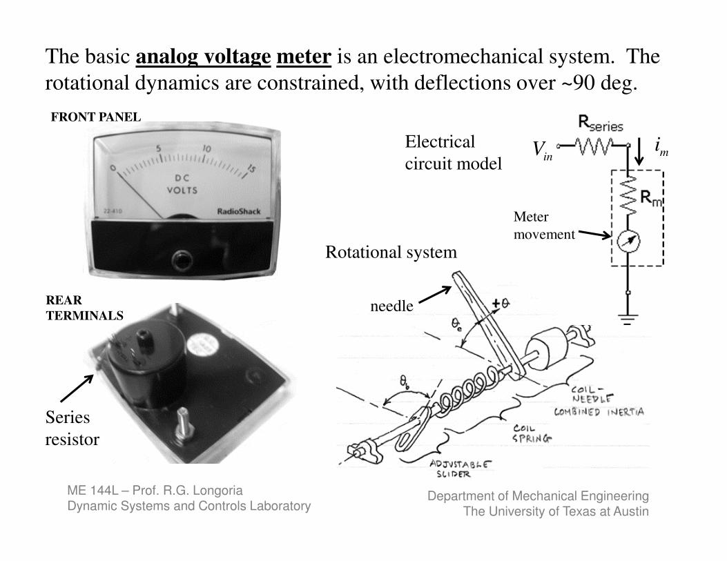
FRONT PANEL

REAR

TERMINALS

Electrical

circuit model

Rotational system

Meter

movement

Series

resistor

needle

The basic analog voltage meter is an electromechanical system. The

rotational dynamics are constrained, with deflections over ~90 deg.

inV mi



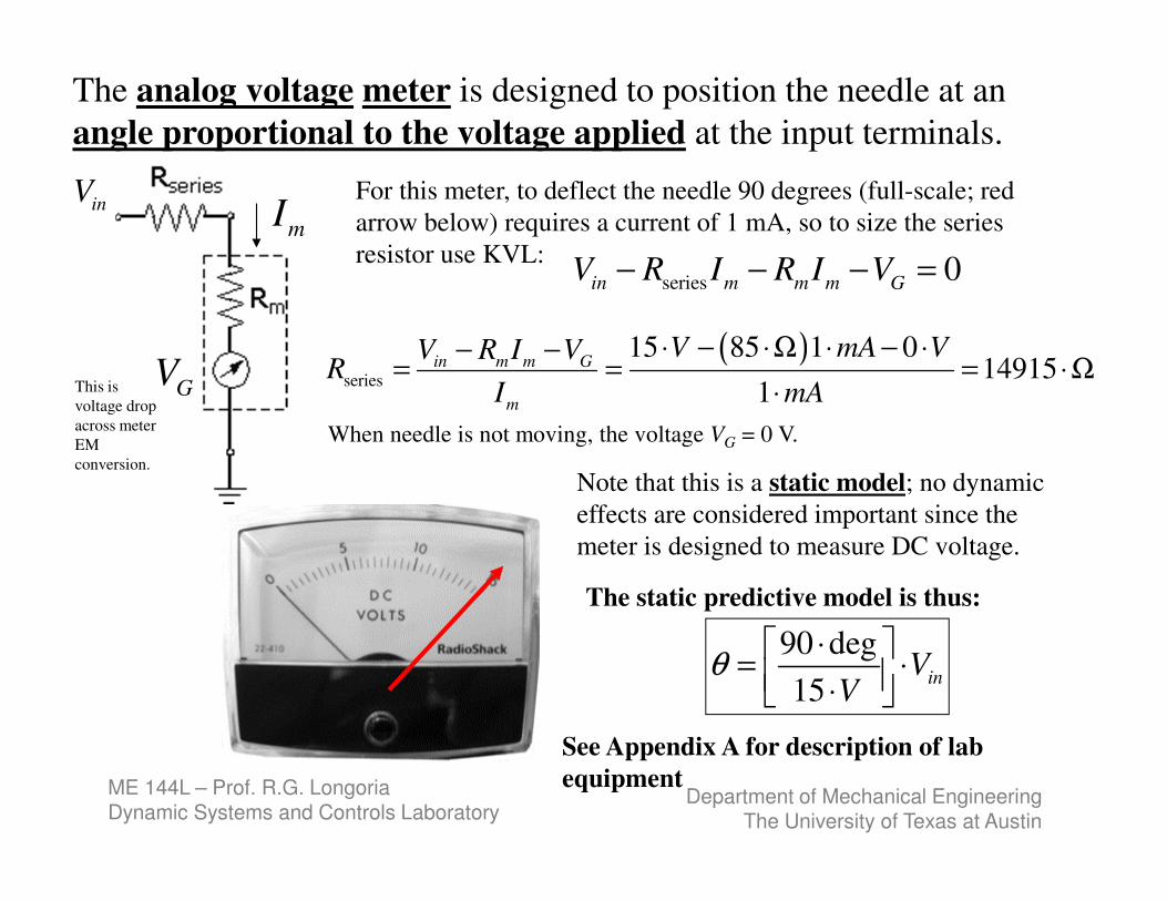
For this meter, to deflect the needle 90 degrees (full-scale; red

arrow below) requires a current of 1 mA, so to size the series

resistor use KVL:

inV

series 0in m m m G

V R I R I V− − − =

( )series

15 85 1 014915

1

in m m G

m

V mA VV R I VR

I mA

⋅ − ⋅Ω ⋅ − ⋅− −= = = ⋅Ω

⋅

Note that this is a static model; no dynamic

effects are considered important since the

meter is designed to measure DC voltage.

GV

mI

90 deg

15in

VV

θ⋅

= ⋅ ⋅

The static predictive model is thus:

See Appendix A for description of lab

equipment

The analog voltage meter is designed to position the needle at an

angle proportional to the voltage applied at the input terminals.

This is

voltage drop

across meter

EM

conversion.

When needle is not moving, the voltage VG = 0 V.



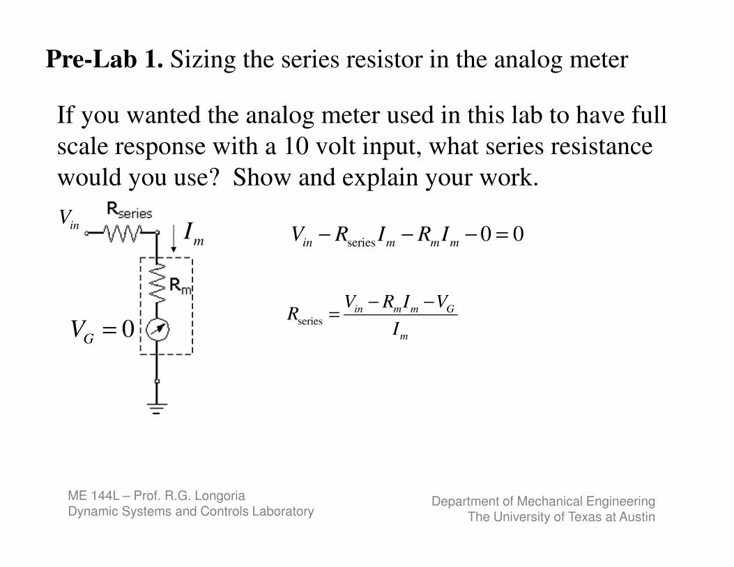
If you wanted the analog meter used in this lab to have full

scale response with a 10 volt input, what series resistance

would you use? Show and explain your work.

Pre-Lab 1. Sizing the series resistor in the analog meter

inV

series 0 0in m m m

V R I R I− − − =

0GV =

mI

seriesin m m G

m

V R I VR

I

− −=



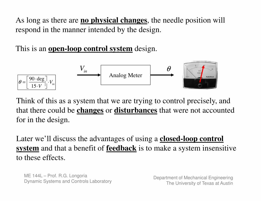
As long as there are no physical changes, the needle position will

respond in the manner intended by the design.

This is an open-loop control system design.

Analog MeterinV θ

Think of this as a system that we are trying to control precisely, and

that there could be changes or disturbances that were not accounted

for in the design.

Later we’ll discuss the advantages of using a closed-loop control

system and that a benefit of feedback is to make a system insensitive

to these effects.

90 deg

15in

VV

θ⋅

= ⋅ ⋅



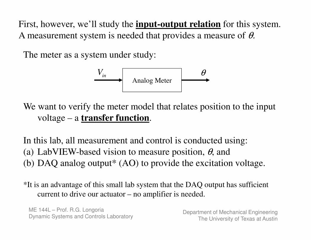
Analog MeterinV θ

First, however, we’ll study the input-output relation for this system.

A measurement system is needed that provides a measure of θ.

The meter as a system under study:

We want to verify the meter model that relates position to the input

voltage – a transfer function.

In this lab, all measurement and control is conducted using:

(a) LabVIEW-based vision to measure position, θ, and

(b) DAQ analog output* (AO) to provide the excitation voltage.

*It is an advantage of this small lab system that the DAQ output has sufficient

current to drive our actuator – no amplifier is needed.



Lab Objectives (1st week)

• Learn how to use LabVIEW for image analysis

and image capture

• Run basic image analysis and image capture

experiments

• Characterize the meter system using a static

gain relating angular position to input voltage

• Demonstrate open-loop control of angular

position



c

θa b

( ),v v

x y

( )0 0,x y ( ),v v

x y

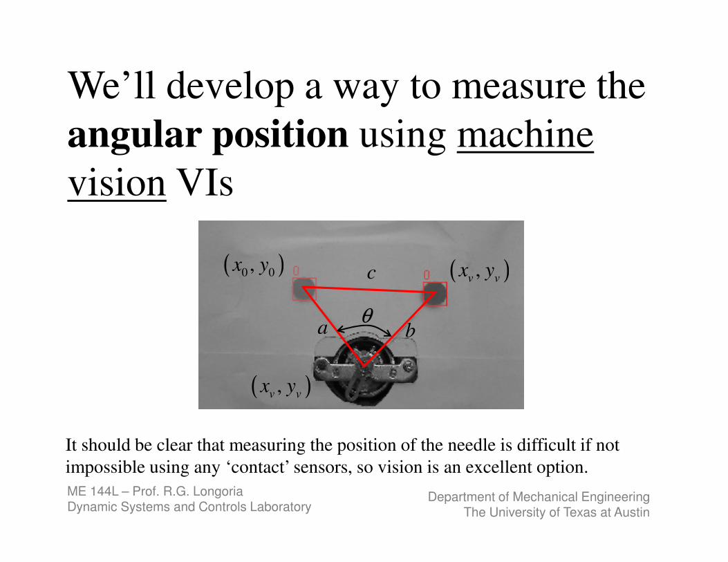
We’ll develop a way to measure the

angular position using machine

vision VIs

It should be clear that measuring the position of the needle is difficult if not

impossible using any ‘contact’ sensors, so vision is an excellent option.



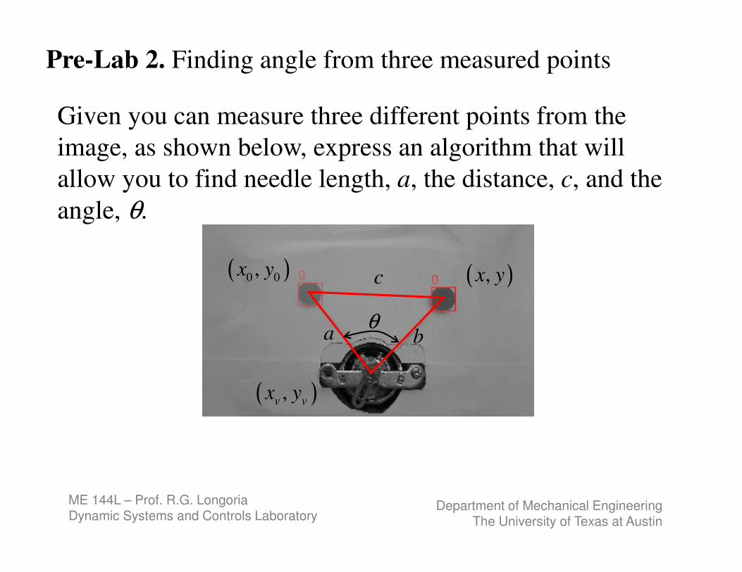
Given you can measure three different points from the

image, as shown below, express an algorithm that will

allow you to find needle length, a, the distance, c, and the

angle, θ.

Pre-Lab 2. Finding angle from three measured points

c

θa b

( ),v v

x y

( )0 0,x y ( ),x y



LabVIEW-based Vision

• LabVIEW Vision enables you to read/create image files and provides means for managing those files

• There are built-in functions (VIs) for analyzing image files (select areas of interest, measure intensity, etc.)

• It is necessary to also have LabVIEW IMAQ software which enables you to acquire images from cameras.

• In this course, we want to demonstrate how you can use these software tools to develop a simple vision-based measurement system, particularly for object motion.



Overview of LV-Based Vision Tools

• Image data type

• Analyzing images

• Capturing images

Vision Utilities

Image processing

Machine vision



Analyzing Images

• Vision Utilities – VIs for creating and

manipulating images, etc.

• Image Processing – provides ‘low level’ VIs

for analyzing images.

• Machine Vision – groups many practical VIs

for performing image analysis. For example,

the “Count and Measure Objects” VI is found

under this group.



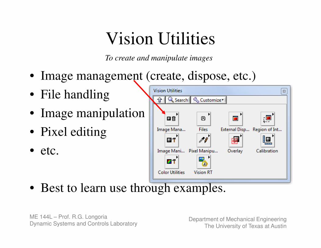
Vision Utilities

• Image management (create, dispose, etc.)

• File handling

• Image manipulation

• Pixel editing

• etc.

• Best to learn use through examples.

To create and manipulate images



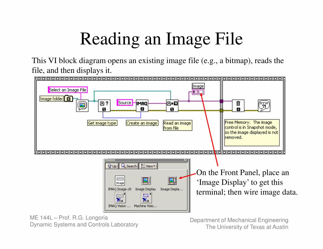
Reading an Image FileThis VI block diagram opens an existing image file (e.g., a bitmap), reads the

file, and then displays it.

On the Front Panel, place an

‘Image Display’ to get this

terminal; then wire image data.



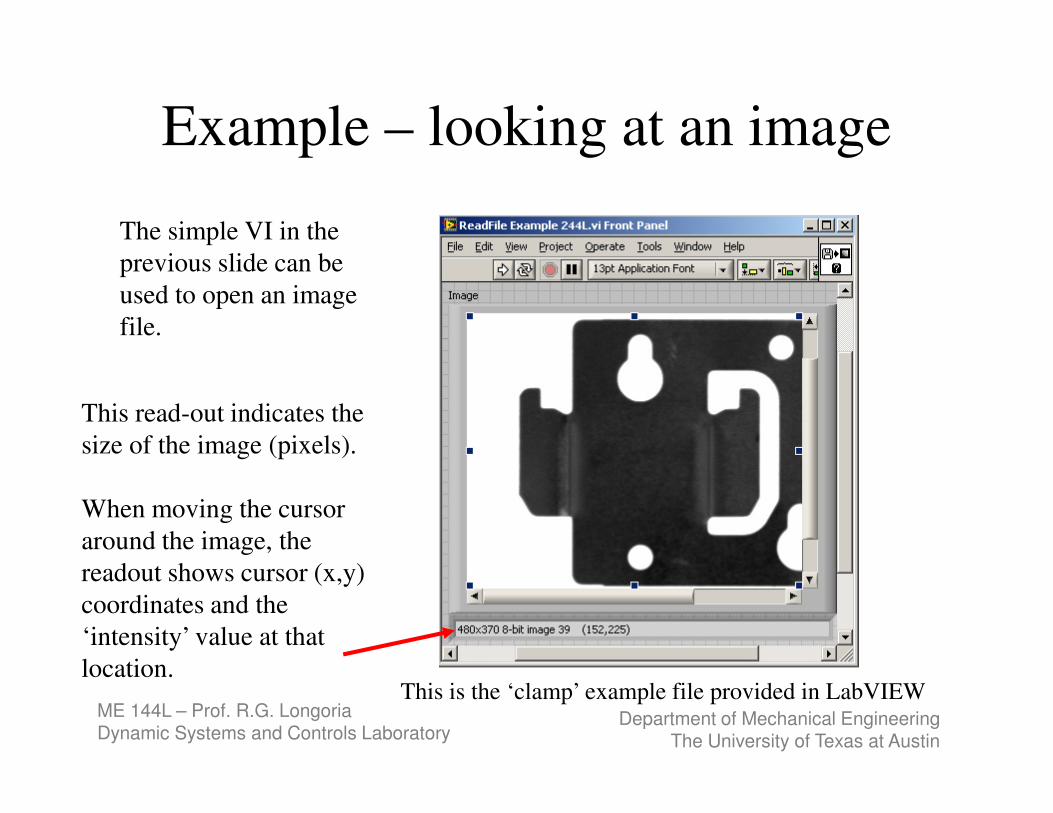
Example – looking at an image

This read-out indicates the

size of the image (pixels).

When moving the cursor

around the image, the

readout shows cursor (x,y)

coordinates and the

‘intensity’ value at that

location.

The simple VI in the

previous slide can be

used to open an image

file.

This is the ‘clamp’ example file provided in LabVIEW



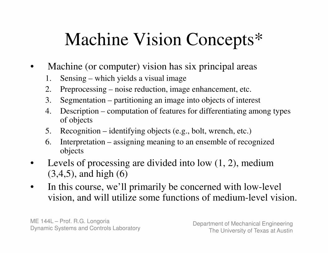
Machine Vision Concepts*

• Machine (or computer) vision has six principal areas

1. Sensing – which yields a visual image

2. Preprocessing – noise reduction, image enhancement, etc.

3. Segmentation – partitioning an image into objects of interest

4. Description – computation of features for differentiating among types of objects

5. Recognition – identifying objects (e.g., bolt, wrench, etc.)

6. Interpretation – assigning meaning to an ensemble of recognized objects

• Levels of processing are divided into low (1, 2), medium (3,4,5), and high (6)

• In this course, we’ll primarily be concerned with low-level vision, and will utilize some functions of medium-level vision.



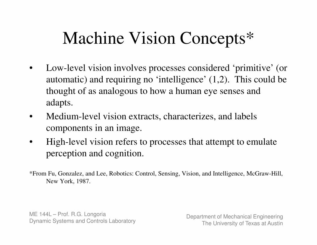
Machine Vision Concepts*

• Low-level vision involves processes considered ‘primitive’ (or

automatic) and requiring no ‘intelligence’ (1,2). This could be

thought of as analogous to how a human eye senses and

adapts.

• Medium-level vision extracts, characterizes, and labels

components in an image.

• High-level vision refers to processes that attempt to emulate

perception and cognition.

*From Fu, Gonzalez, and Lee, Robotics: Control, Sensing, Vision, and Intelligence, McGraw-Hill,

New York, 1987.



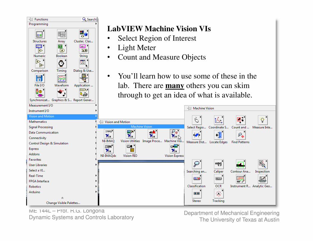
LabVIEW Machine Vision VIs

• Select Region of Interest

• Light Meter

• Count and Measure Objects

• You’ll learn how to use some of these in the

lab. There are many others you can skim

through to get an idea of what is available.



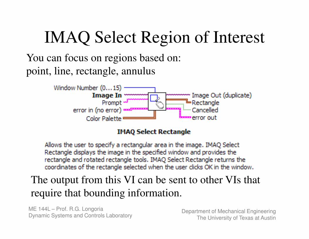
IMAQ Select Region of InterestYou can focus on regions based on:

point, line, rectangle, annulus

The output from this VI can be sent to other VIs that

require that bounding information.



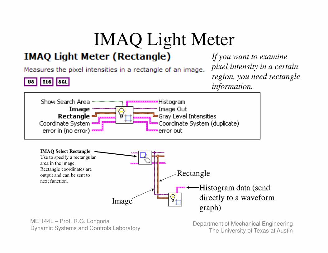
IMAQ Light Meter

IMAQ Select Rectangle

Use to specify a rectangular

area in the image.

Rectangle coordinates are

output and can be sent to

next function.

Image

Rectangle

Histogram data (send

directly to a waveform

graph)

If you want to examine

pixel intensity in a certain

region, you need rectangle

information.



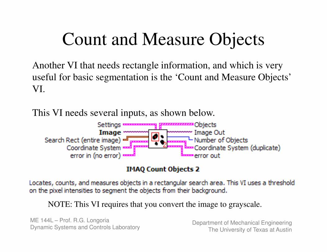
Count and Measure Objects

Another VI that needs rectangle information, and which is very

useful for basic segmentation is the ‘Count and Measure Objects’

VI.

This VI needs several inputs, as shown below.

NOTE: This VI requires that you convert the image to grayscale.



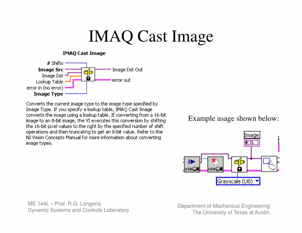
IMAQ Cast Image

Example usage shown below:



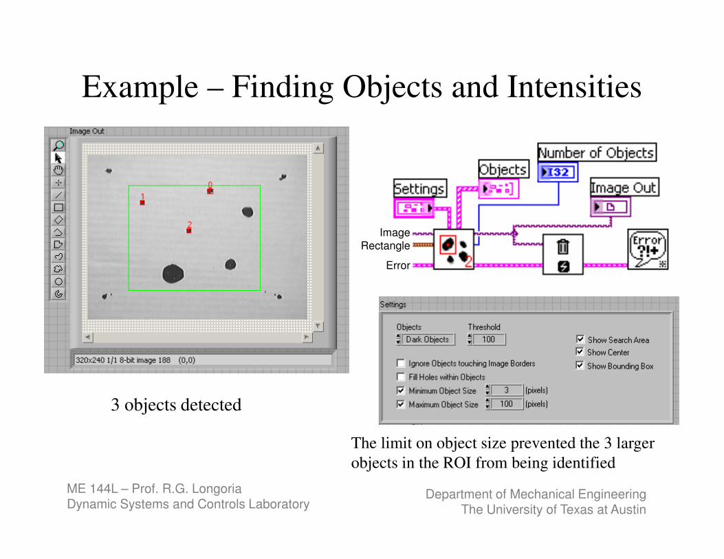
Example – Finding Objects and Intensities

3 objects detected

Image

Rectangle

Error

The limit on object size prevented the 3 larger

objects in the ROI from being identified



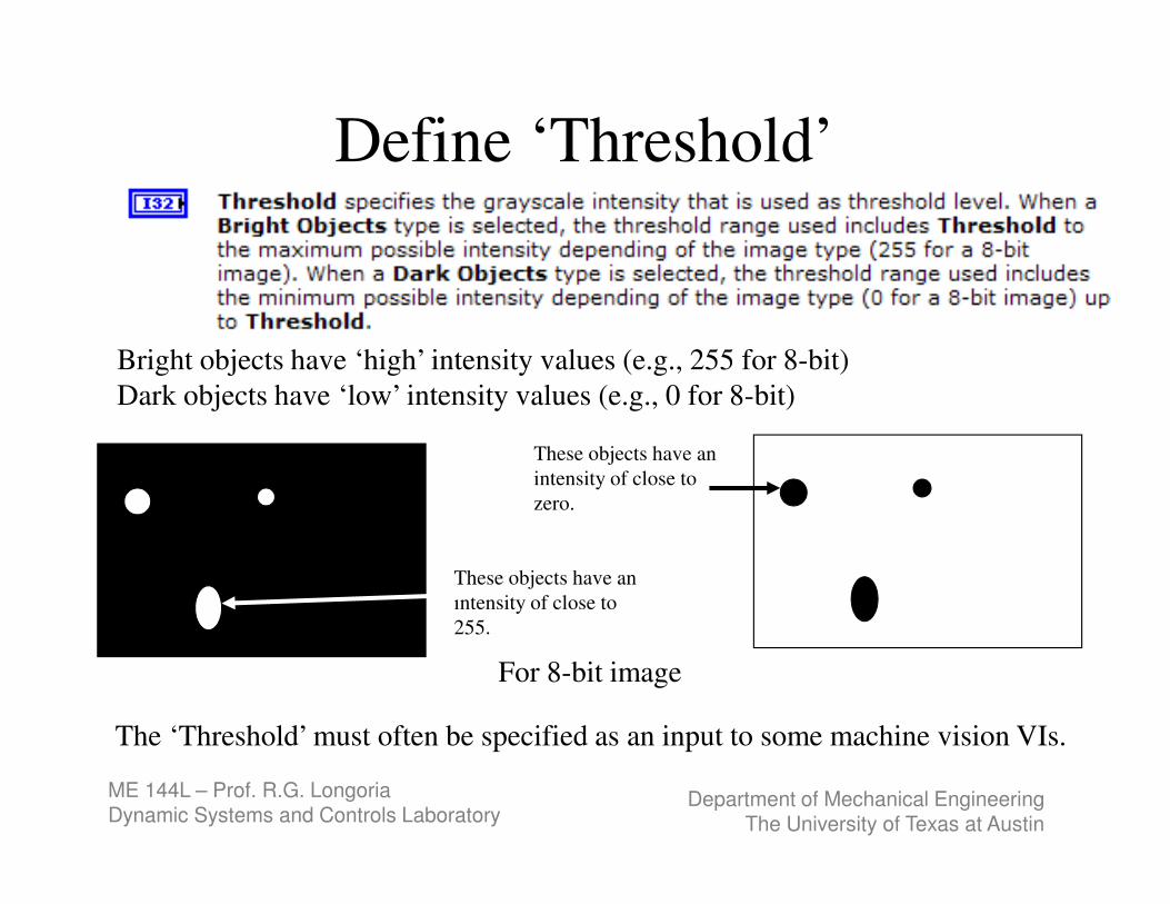
Define ‘Threshold’

These objects have an

intensity of close to

zero.

These objects have an

intensity of close to

255.

For 8-bit image

Bright objects have ‘high’ intensity values (e.g., 255 for 8-bit)

Dark objects have ‘low’ intensity values (e.g., 0 for 8-bit)

The ‘Threshold’ must often be specified as an input to some machine vision VIs.



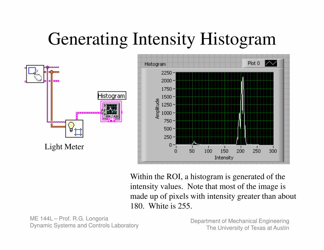
Generating Intensity Histogram

Light Meter

Within the ROI, a histogram is generated of the

intensity values. Note that most of the image is

made up of pixels with intensity greater than about

180. White is 255.



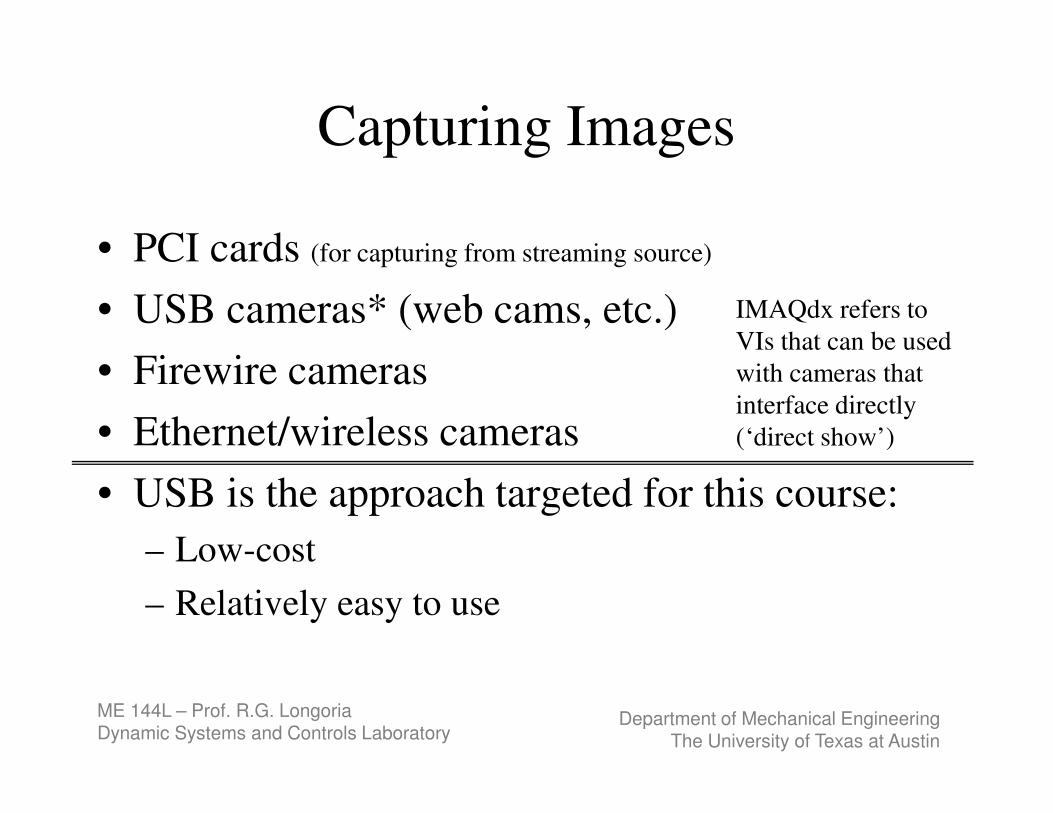
Capturing Images

• PCI cards (for capturing from streaming source)

• USB cameras* (web cams, etc.)

• Firewire cameras

• Ethernet/wireless cameras

• USB is the approach targeted for this course:

– Low-cost

– Relatively easy to use

IMAQdx refers to

VIs that can be used

with cameras that

interface directly

(‘direct show’)



USB Cameras

• USB cameras are probably the slowest cameras available, especially the way they are to be used in this course.

• Our experience has shown that the maximum bandwidth we can achieve for image acquisition is about 10 frames/sec (within LabVIEW).

• Some online sources indicate that ‘hacked’ webcams can achieve 30 frames/sec.

• So, it is the software environment (Windows, LV, communications, etc.) that we’ve chosen that is likely placing the restrictions on the performance.



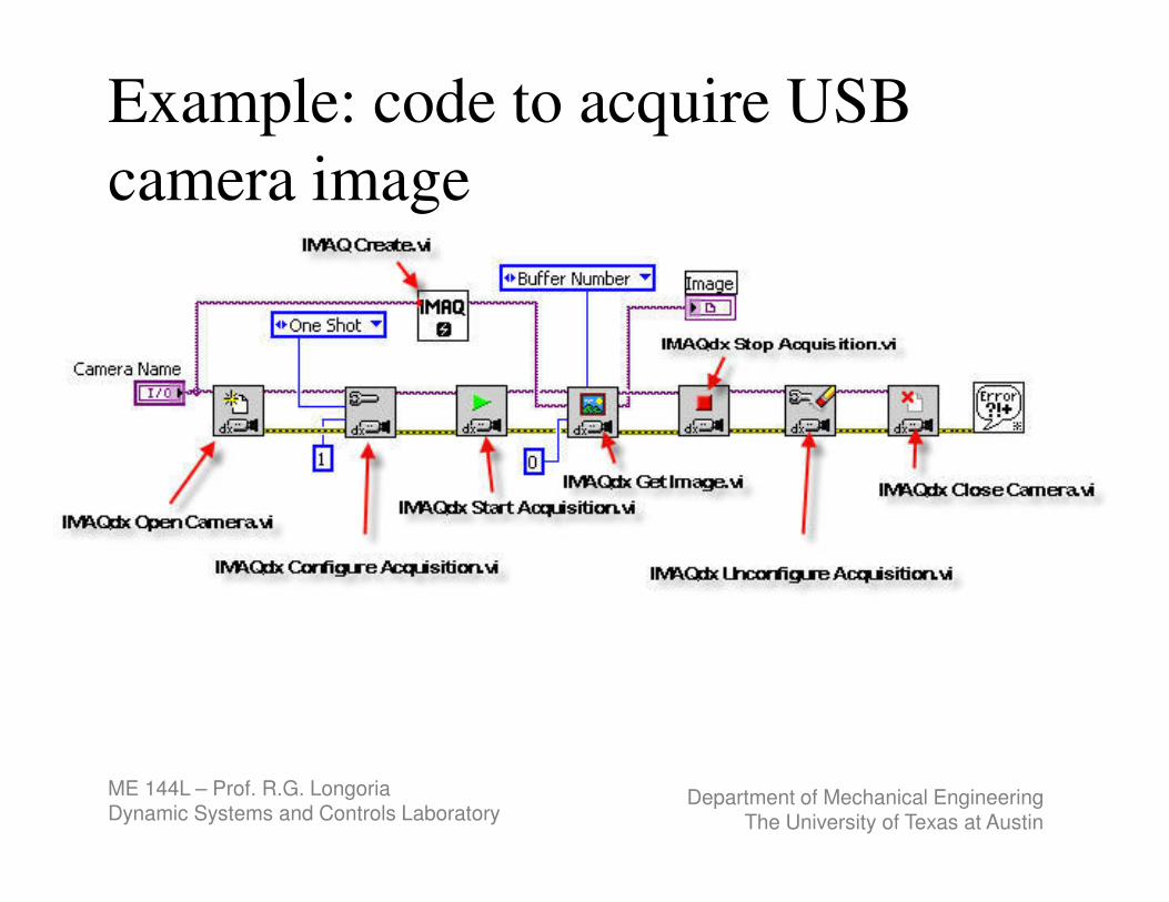
Example: code to acquire USB

camera image



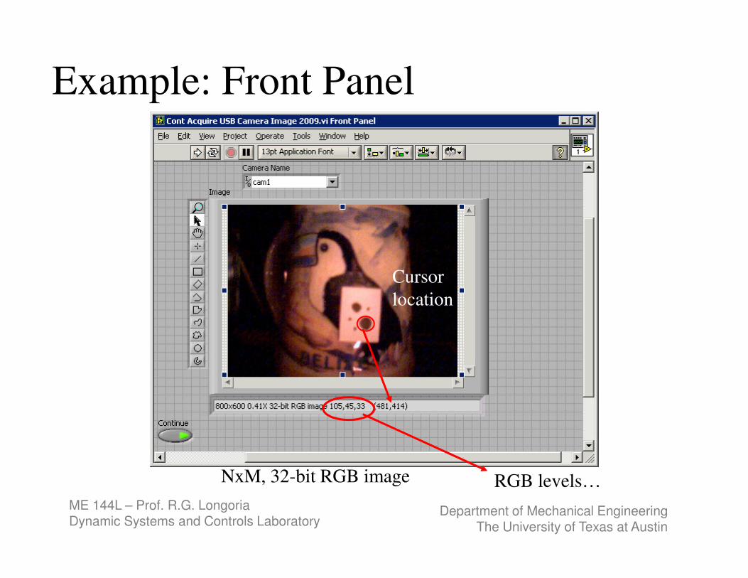
Example: Front Panel

NxM, 32-bit RGB image RGB levels…

Cursor

location



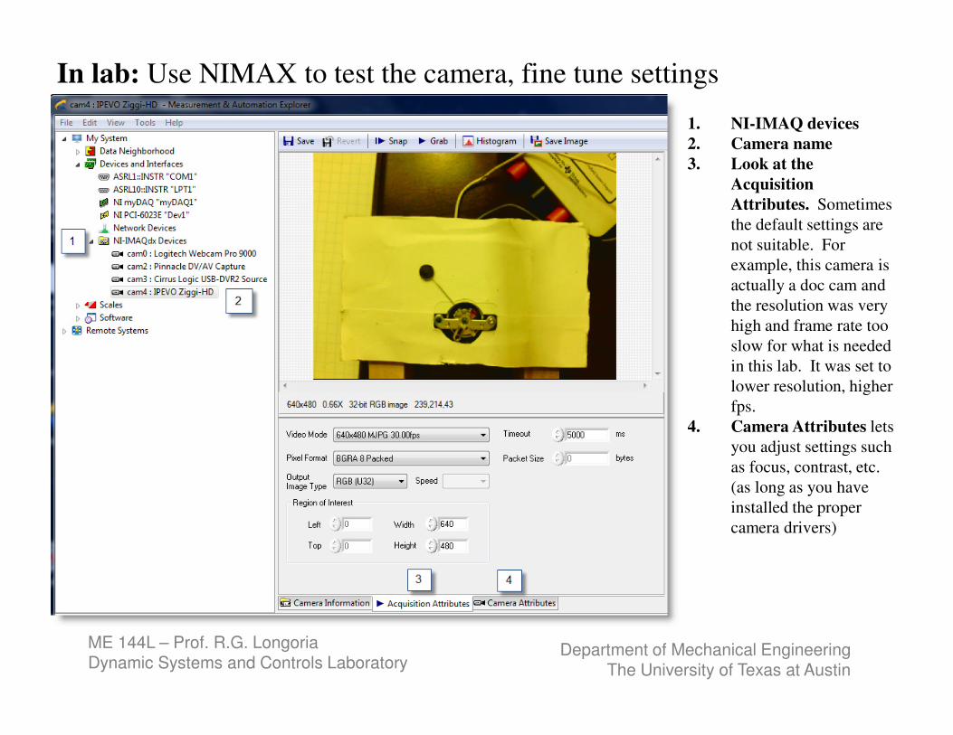
In lab: Use NIMAX to test the camera, fine tune settings

1. NI-IMAQ devices

2. Camera name

3. Look at the

Acquisition

Attributes. Sometimes

the default settings are

not suitable. For

example, this camera is

actually a doc cam and

the resolution was very

high and frame rate too

slow for what is needed

in this lab. It was set to

lower resolution, higher

fps.

4. Camera Attributes lets

you adjust settings such

as focus, contrast, etc.

(as long as you have

installed the proper

camera drivers)



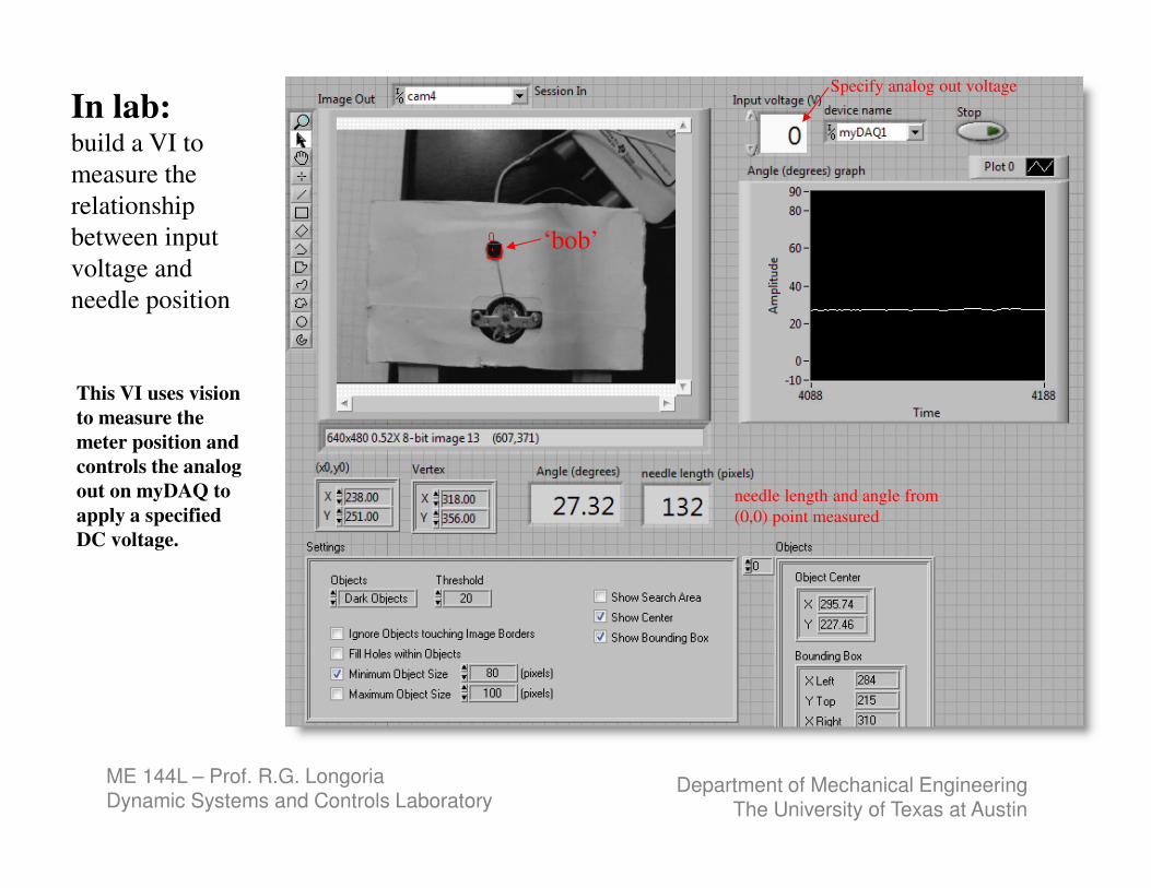
This VI uses vision

to measure the

meter position and

controls the analog

out on myDAQ to

apply a specified

DC voltage.

Specify analog out voltage

In lab:build a VI to

measure the

relationship

between input

voltage and

needle position

‘bob’

needle length and angle from

(0,0) point measured



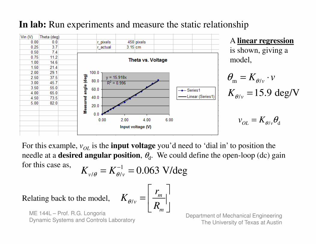
m /

/ 15.9 deg/V

v

v

K v

K

θ

θ

θ = ⋅

=

A linear regression

is shown, giving a

model,

/ dOL vv Kθ θ=

For this example, vOL is the input voltage you’d need to ‘dial in’ to position the

needle at a desired angular position, θd. We could define the open-loop (dc) gain

for this case as,

In lab: Run experiments and measure the static relationship

1

/ / 0.063 V/degv v

K Kθ θ

−= =

/m

v

m

rK

Rθ

=

Relating back to the model,



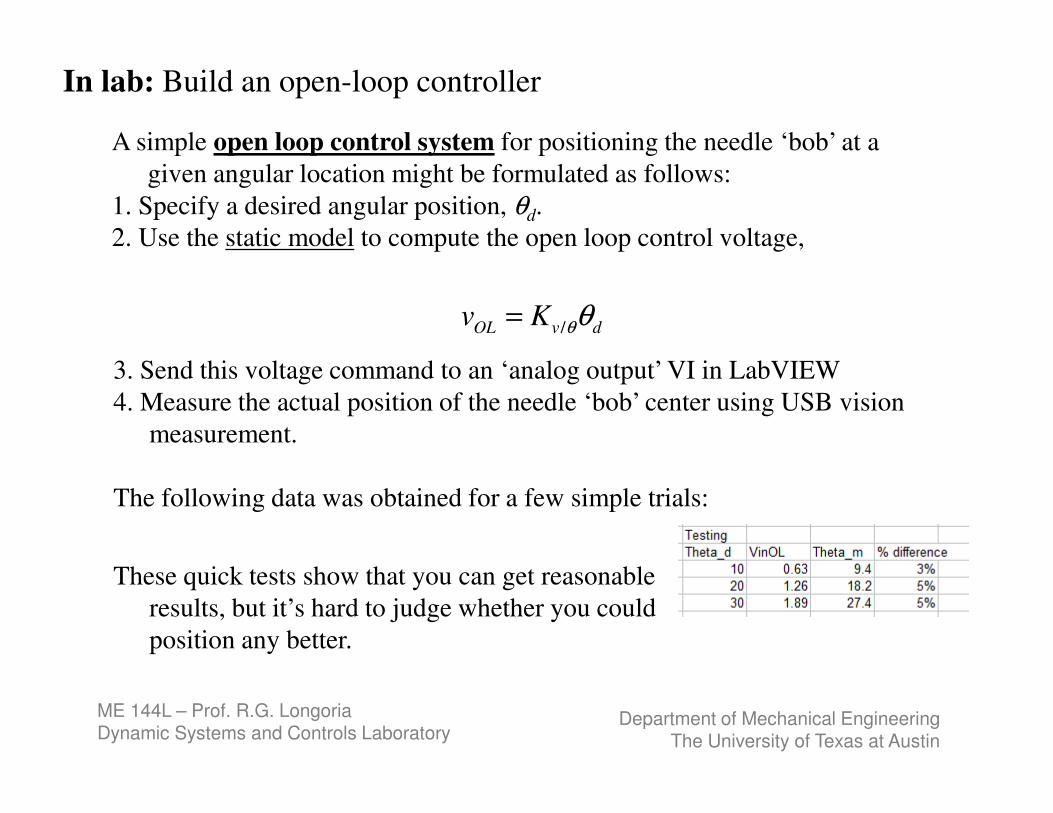
/OL v dv K θθ=

A simple open loop control system for positioning the needle ‘bob’ at a

given angular location might be formulated as follows:

1. Specify a desired angular position, θd.

2. Use the static model to compute the open loop control voltage,

3. Send this voltage command to an ‘analog output’ VI in LabVIEW

4. Measure the actual position of the needle ‘bob’ center using USB vision

measurement.

The following data was obtained for a few simple trials:

These quick tests show that you can get reasonable

results, but it’s hard to judge whether you could

position any better.

In lab: Build an open-loop controller



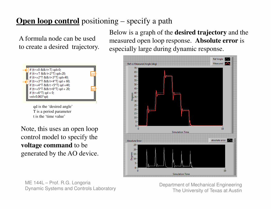
A formula node can be used

to create a desired trajectory.

Note, this uses an open loop

control model to specify the

voltage command to be

generated by the AO device.

Below is a graph of the desired trajectory and the

measured open loop response. Absolute error is

especially large during dynamic response.

Open loop control positioning – specify a path

qd is the ‘desired angle’

T is a period parameter

t is the ‘time value’



Summary

• We begin study of an electromechanical analog meter

• Vision VIs in LabVIEW provide a way for us to include image acquisition and analysis to our existing set of tools (simulation, DAQ).

• The vision VIs alone allow you to use an image as a data type.

• Images can be loaded from a file or acquired using IMAQ routines.

• Once within LabVIEW, an image can be processed using some very sophisticated built-in programs.

• Machine vision VIs enable us to build a simple ‘motion capture’ system for studying the analog meter response and control.



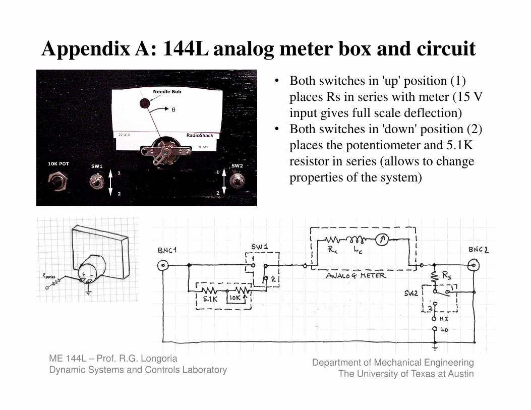
Appendix A: 144L analog meter box and circuit

• Both switches in 'up' position (1)

places Rs in series with meter (15 V

input gives full scale deflection)

• Both switches in 'down' position (2)

places the potentiometer and 5.1K

resistor in series (allows to change

properties of the system)



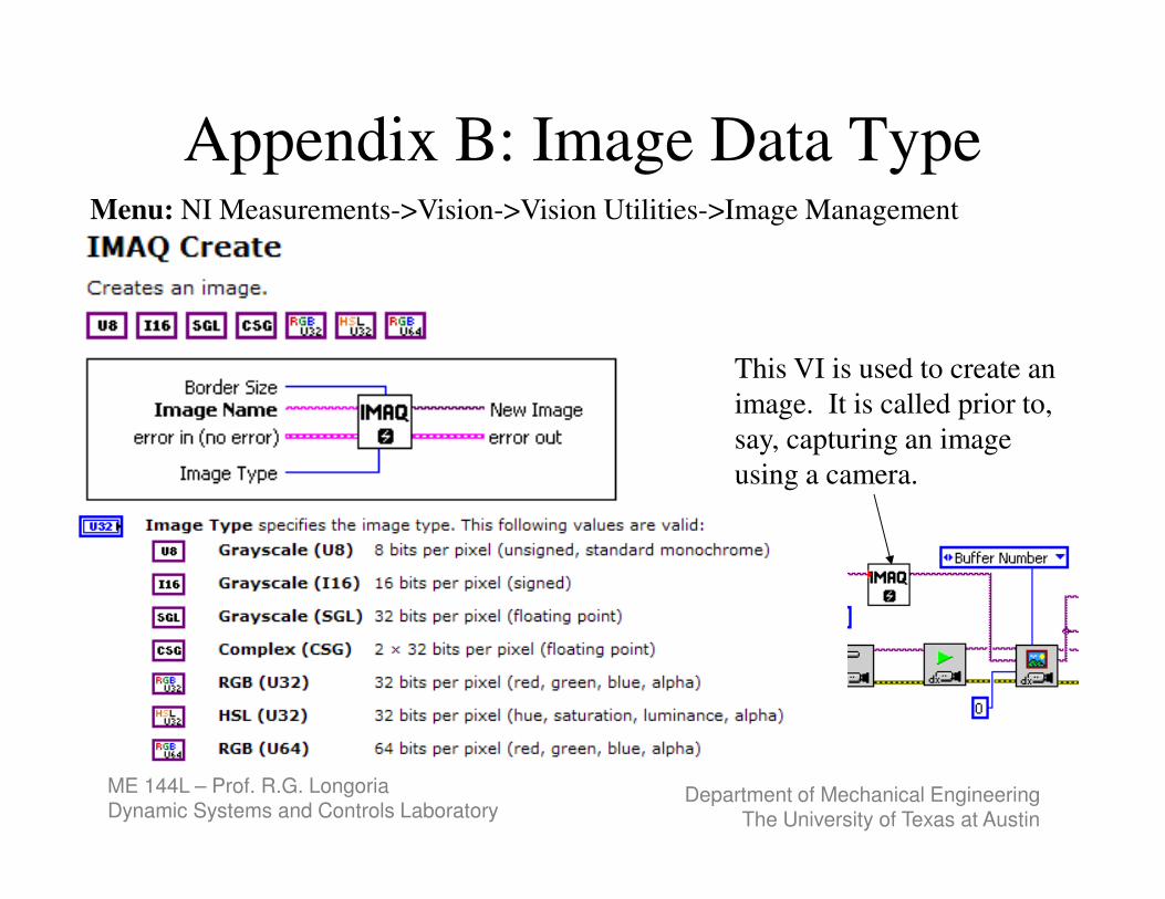
Appendix B: Image Data TypeMenu: NI Measurements->Vision->Vision Utilities->Image Management

This VI is used to create an

image. It is called prior to,

say, capturing an image

using a camera.



Appendix C: Image Type and Bit Depth

• We know digital images are formed by an array of pixels, and each pixel is quantized into a number of levels based on the number of bits available.

• Depending on whether pixels are black and white, grayscale, or color, pixels have different bit depths. Bit depth refers to the amount of information allocated to each pixel.

• When pixels are either black or white, pixels need only two bits of information (black or white), and hence the pixel depth is 2.

• For grayscale, the number of levels used can vary but most systems have 256 shades of gray, 0 being black and 255 being white. When there are 256 shades of grey, each pixels has a bit depth of 8 bits (one byte). A 1024 x 1024 grayscale images would occupy 1MB of memory.

• In digital color images, the RGB (red green blue, for screen projection) or CMYK (printing color) schemes are used. Each color occupies 8 bits (one byte), ranging in value from 1-256. Hence in RGB each pixel occupies 8x3 =24 (3 bytes) bits, in CMYK 8x4 = 32 bits (4 bytes).

• Note, LV uses an ‘alpha’ channel for RGB. The alpha channel stores transparency information--the higher the value, the more opaque that pixel is.

Documents

Studying Analog Meter System using LabVIEW …dsclab/leks/DSC_Meter_and_LabVIEW_Vision.pdf · (a) LabVIEW-based vision to measure position, θ, and (b) DAQ analog output* (AO) to