Embed Size (px)
Citation preview
Republic of Iraq
Ministry of Higher Education
and scientific Research
University of Al-Qadisiyah
College of Education
Study the Mechanical Properties of SiC
Material by Using Molecular Dynamic
Simulation (lammps)
A Thesis Submitted to
the Council of the College of Education – Al-Qadisiyah
University
In Partial Fulfillment of the Requirements for the Degree of
Master of Science in Physics
Submitted by
Shurooq Hayder Abd alnebee Al-mehanyah
Supervised by
Assistant Professor
Dr. Hisham Mohammed ali Hasan AL-Barmany
2017 A.D 1438 A.H

أ
ه عع ا يههنو اععهوالل الل اهذ عع يرفعع الله
عع ه عع ها يههواوواععهذمالل الل وذ عع
نهخباللير ه اهباللم هومم ا وه
العظيم العلي صدق الله
المجادلة سورة
(11)الآية ه


iii
Abstract
In this thesis, the crack and modified embedded atom method
(MEAM) by using molecular dynamics simulation was studied, simulator
(lammps) of crack propagation in hexagonal lattice and in modified
embedded atom method (MEAM) for material silicon carbide )SiC). The
mechanisms of crack including emission of dislocations and creation of
stacking faults.
In crack code the time steps used was (0.044,0.04,0.03, 0.02, 0.01,
0.009, 0.008, 0.007, 0.006, 0.005, 0.004, 0.003, 0.002, 0.001and 0.00001
tau( and in modified embedded atom method code time steps used was
(0.003, 0.002, 0.001, 0.0009, 0.0008, 0.0007, 0.0006, 0.0005 and 0.0001
Ps(, the time step must be chosen small enough to ensure energy
conservation and to avoid large discretization errors, so the best choice
time step in crack was (0.00001 reduced( and in Modified Embedded
Atom Method (MEAM) is (0.0001 Ps(. In crack code increase (decreases
in negative) potential energy because the crack was not initiated, while
the crack initiate at step (run) =10600, while potential energy was (-
3.2511ϵ) at step (run) =10600 resulting by breaking the bonds between
atoms while the increase in temperature indicates that the crack
propagated. The increase )decreases in negative( pressure of the system
because there is no crack initiation, then decreases )increasing in
negative( pressure resulting from breaking the bonds between atoms at
crack propagation. In this code the volume or area of crack is constant.
In Modified Embedded Atom Method (MEAM) the increases in
negative potential energy because the embedded atom within the group
of atoms (stable system) need sufficient energy in order to break the
bonds between the atoms. And the increases of the kinetic energy of the

iv
system can be attributed to the rapid breaking. Although the energy of
the system is conserved, the temperature will increase when potential
energy is transferred into thermal kinetic energy , resulting in breaking
the bonds between atoms. And an increases in negative pressure result of
breaking the bonds between atoms.

v
LIST OF CONTENTS
Subject Page
Dedication i
Acknowledgments ii
Abstract iii
List of contents v
List symbol of Abbreviation viii
List of Tables xiii
List of Figures xiii
CHAPTER I: Introduction
1-1 Introduction 1
1-2 Literature Review 5
1-3 The goal 8
CHAPTER II: Molecular Dynamics Simulation
2-1 Molecular interactions 9
2-1-1 Non-bonded Potential Energy 9
2-1-2 Bonding Potentials 12
2-1-2-1 The Bond Length 14
2-1-2-2 The Bond Angles 15
2-1-2-3 The Torsion Angles 17
2-2 The Molecular Dynamics (MD) Algorithm 18
2-2-1 The Verlet Algorithm 19
2-2-2 Common Neighbor Analysis Approach 20
2-2-3 Schematic of the Molecular Dynamics (MD) Algorithm 22
2-3 Molecular Dynamics in Different Ensembles 23

vi
2-3-1 Micro-Canonical or NVE Ensemble 23
2-3-2 Canonical or NVT Ensemble 24
2-3-3 Isothermal-Isobaric or NPT Ensemble 24
CHAPTER III: Theoretical part
3-1 Quantum Many-Body Problem 25
3-1-1 The Born-Oppenheimer Approximation 26
3-1-2 The Variational Principle 28
3-2 Density Functional Theory 29
3-2-1 Hohenberg and Kohn (H-K) Theorems 29
3-2-2 Kohn-Sham (K-S) Equation 31
3-2-3 Functionals for Exchange and Correlation 32
3-2-3-1The Local Density Approximation )LDA) 33
3-2-3-2 The Generalized Gradient Approximation (GGA) 33
3-2-4 Pseudopotentials 34
3-2-4-1 Frozen Core Approximation 34
3-2-4-2 Formal Justification for Pseudopotentials 35
3-2-4-3 Different Approaches for Pseudopotentials 36
3-2-4-3-1 Norm- Conserving Pseudopotentials (NC-PP) 37
3-2-4-3-2 Ultrasoft Pseudopotentials (US-PP) 38
3-2-4-3-3 Projector Augmented Waves (PAW) 39
3-3 Embedded Atom Method (EAM) 40
3-4 Modified Embedded Atom Method (MEAM) 43
3-5 Molecular dynamics (MD) Modeling of Fracture 47
3-5-1 Model potentials for Brittle Materials 47
3-5-2 Model Geometry and Simulation Procedure 55
CHAPTER IV: RESULTS & DISCUSSION
4-1 Crack code 51

vii
4-2 Modified Embedded Atom Method (MEAM) code 64
4-3 Conclusions 71
4-4 Future works 71
Appendix I LAMMPS
1-1 An introduction to LAMMPS 72
1-2 Installing LAMMPS 72
1-2-1 Installing LAMMPS on Windows 73
1-2-2 Installing LAMMPS on Ubuntu 73
1-3 Running LAMMPS 75
1-3-1 Running LAMMPS on Windows 75
1-3-2 Running LAMMPS on Ubuntu 76
1-4 Simulation Procedures 77
1-4-1 Procedures 77
1-4-2 Output of Simulation 77
1-5 Thermodynamic Properties in LAMMPS 78
1-5-1 Number of Particles of Component i, Ni 78
1-5-2 Volume of the system, V 79
1-5-3 Temperature, T 79
1-5-4 Pressure, P 79
1-5-5 Kinetic energy, KE 81
1-5-6 Potential energy, PE 82
1-5-7 Internal energy, U (or total energy, E) 82
1-6 Working with LAMMPS 83
1-6-1 input script in Crack 84
1-6-1-1 Initialization 84
1-6-1-2 Atom, and lattice definition 85
1-6-1-3 Force fields 86

viii
1-6-1-4 Settings 87
89
1-6-1-5 Run the Simulator
1-6-2 Input script in MEAM 91
1-6-2-1 Initialization 91
1-6-2-2 Atom definition 92
1-6-2-3 Force fields 93
1-6-2-4 Run the simulator 93
References 95
LIST SYMBOL OF ABBREVIATION
The symbol The meaning of the symbol Unit
reduced
Unit
metal
MD Molecular Dynamics
EAM Embedded Atom Method
MEAM Modified Embedded Atom Method
FCC Face Centered Cubic
BCC Body Centered Cubic
HCP Hexagonal Close Packing
MC Monte Carlo
LAMMPS Large-scale Atomic/Molecular Massively
Parallel Simulator
CNA Common Neighbor Analysis
CTMD Constant Temperature Molecular
Dynamics

ix
DFT Density Functional Theory
H-K Hohenberg and Kohn
K-S Kohn-Sham
LDA Local Density Approximation
GGA Generalized Gradient Approximation
PAW projector-augmented wave
OPWs Orthogonalized plane waves
NC-PP Norm-Conserving Pseudopotentials
US-PP Ultrasoft Pseudopotentials
LJ Lennard-Jones
NVE
(constant number of particles, constant
volume, constant energy) microcanonical
ensemble
NVT
(constant number of particles, constant
volume, constant temperature) canonical
ensemble
NPT
constant number of particles, constant
pressure, constant temperature)
isothermal–isobaric ensemble
Fi Force of atom (i)
mi Mass of atom (i) m
ai Acceleration of atom (i)
vi Velocity of atom (i)
ri Position of atom (i)
R, r Distance between the two atoms, Bond Angstroms

x
length
Well depth
The charges
Permittivity of free space
, Bond length
Equilibrium bond length
, Angle spring
, Bond angles
Equilibrium angle
, Torsion angle
p Momentum
H Energy or hamiltouian
k Kinetic energy eV
U Potential energy eV
t Time tau picosecond
, Time step tau picosecond
E, E* Total energy eV
V Volume Cm3
N Number of atoms
T Temperature
Kelvin
Hamiltonian
Represents the kinetic energy and the
interaction of the nuclei
Represents the interaction between the
electron and nuclei
Represents the interaction between the
xi
electrons
h Plank constant
Mass of nuclei
Charges of the nucleus
e Charge of the electron
Radius of nucleus
Radius of electron
, Wave function
Wave function of the nuclei
The operator for the kinetic energy
The potential acting on the electrons due
to the nuclei
The electron-electron interaction
The interaction of the nuclei
The expectation value of an operator
n(r) The particle density
Hartree energy
VXC The exchange-correlation potential
Exchange-correlation energy density
⟩ The pseudo wave function
⟩ The core wave functions
Fi , Embedding functional
The contribution of the atom( j) of type
(a) to the electron charge density
𝑗 The distance between atoms (i) and( j)
𝜙 𝑗 The short-range pair potential
Z The atomic number of the atoms
xii
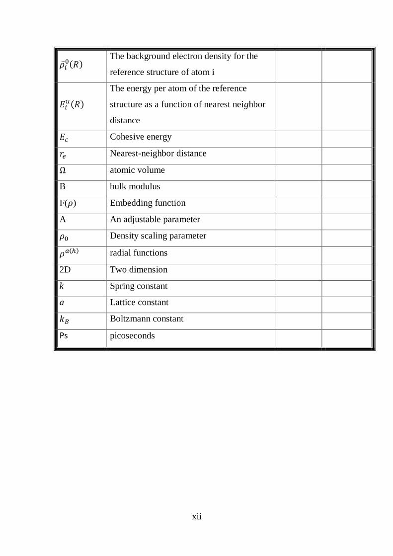
( )
The background electron density for the
reference structure of atom i
( )
The energy per atom of the reference
structure as a function of nearest neighbor
distance
Cohesive energy
Nearest-neighbor distance
atomic volume
B bulk modulus
F( ) Embedding function
A An adjustable parameter
Density scaling parameter
( ) radial functions
2D Two dimension
k Spring constant
a Lattice constant
Boltzmann constant
Ps picoseconds

xiii
LIST OF TABLES
Subject Page
Table 4-1: Total energy vs. step (run) at run 5000 in crack 53
Table 4-2: Values of the crack at time step 0.00001tau and run 18000 56
Table 4-3 : Total energy vs. step (run) in MEAM 64
Table 4-4: Values of the MEAM at time step 0.0001 Ps 66
LIST OF FIGARES
Subject Page
2-1 Lennard-Jones potential 11
2-2 Geometry of a simple chain molecule, illustrating the definition
of interatomic distance , bend angle , and torsion angle 13
2-3 The bond length 15
2-4 The bond angles 16
2-5 The torsion angles 17
2-6 Illustration of several common neighbor atoms structure in
different lattice type. 21
xiv
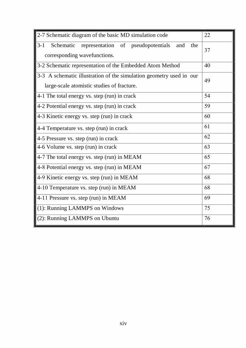
2-7 Schematic diagram of the basic MD simulation code 22
3-1 Schematic representation of pseudopotentials and the
corresponding wavefunctions. 37
3-2 Schematic representation of the Embedded Atom Method 45
3-3 A schematic illustration of the simulation geometry used in our
large-scale atomistic studies of fracture. 49
4-1 The total energy vs. step (run) in crack 54
4-2 Potential energy vs. step (run) in crack 59
4-3 Kinetic energy vs. step (run) in crack 65
4-4 Temperature vs. step (run) in crack 61
4-5 Pressure vs. step (run) in crack 62
4-6 Volume vs. step (run) in crack 63
4-7 The total energy vs. step (run) in MEAM 65
4-8 Potential energy vs. step (run) in MEAM 67
4-9 Kinetic energy vs. step (run) in MEAM 68
4-15 Temperature vs. step (run) in MEAM 68
4-11 Pressure vs. step (run) in MEAM 69
(1): Running LAMMPS on Windows 75
(2): Running LAMMPS on Ubuntu 76

CHAPTER ONE INTRODUCTION

Introduction .................................................................... chapter one
1
1-1 Introduction
Molecular dynamics (MD) is a computer program simulation
method ( installation of program and the input data in appendix I) , for
examining the physical movements of N-atoms and molecules [1], the
atoms and molecules are allowed to interact for a fixed period of time [2],
the equations of motion for a system of interacting particles are
determined by numerically solved Newton's equations,
where forces between the particles and their potential energies are
calculated using interatomic potentials or molecular mechanics force
fields [3]. Molecular dynamics (MD) simulation have been widely used
in various academic fields, such as physics, biophysics, chemistry, and
materials science [1].
Molecular dynamics (MD) is one of the first simulation methods has
been applied to study the dynamics of liquids by Alder, Wainwright [4]
and by Rahman [5] in the late 1950 and early 1960. Molecular dynamics
(MD) has become an important tool in many areas of physics. Since the
1970 molecular dynamics (MD) has been used widely to study the
structure and dynamics of macromolecules, such as crack or fracture
and Modified Embedded Atom Method (MEAM) [6].
Molecular dynamics (MD) simulations use to understanding the
properties of assemblies of molecules in terms of their structure and the
microscopic interactions between them. Computer simulations act as a
bridge between microscopic length and time scales and the macroscopic
world of the laboratory, Molecular dynamics (MD) provide a guess at the
interactions between molecules, and obtain `exact' predictions of bulk
properties [7] .
The molecular dynamics (MD) simulation is being used for
investigating physical in the field of solid-state physics (metal structure

Introduction .................................................................... chapter one
2
conversion, cracks initiated by pressure and shear stresses, and fracture)
and fluid dynamics [8]. Molecular dynamics (MD) runs in crack
propagation or fracture, Modified Embedded Atom Method (MEAM),
flow, body, balance, colloid, deposit, dipole, friction, melt and shear, in
this thesis used crack and Modified Embedded Atom Method (MEAM).
Fracture is the separation of a body into two or more pieces in
response to an stress .The applied stress which may be tensile,
compressive, shear, or torsional. There are two fracture modes; ductile
and brittle. Ductile materials typically exhibit substantial plastic
deformation with high energy absorption before fracture while brittle
fracture is normally little or no plastic deformation with low energy
absorption [9].
Fracture normally occurs through the enlargement of existing
defects, in solid voids, grain boundaries, or micro-cracks, all such defects
concentrate stress,the fact that failure stresses lie far below ideal crystal
strengths shows that the stress concentration is large [10]. Apply the
embedded atom method to basic parts of the fracture process sach as
dislocation dynamics, and crack tip plasticity [11].
The embedded atom method (EAM), developed by Daw and Baskes
[12,13] in the early 1980, is a semi-empirical N-body potential useful for
the atomistic simulations of metal systems. It has successfully been
utilized to calculate the energetics and structures of complex metallic
systems involving free surfaces, defects and grain boundaries [14,15].
The embedded atom method (EAM) construction is based on the use
of density functional theory, in which the energy of a collection of atoms
can be expressed exactly by function of its electronic density. In the
embedded atom method (EAM), each atom is embedded in a host
electron gas created by its neighboring atoms. The atom host interaction
Introduction .................................................................... chapter one
3
is described using the embedding function incorporating some important
many-atom interactions. It is possible to describe and understand
interatomic interactions at defects in terms of either the embedding
function or the effective many-atom interactions that arise from it.
Embedded atom method (EAM) potentials have been applied to study
many aspects of materials behavior in face centered cubic (fcc), body
centered cubic (bcc) and hexagonal close packing (hcp) metals . Although
the embedded atom method (EAM) gives a more detals of crystal
properties than can be obtained by pair potentials, there are two
assumptions, first, spherically averaged free atom densities represent the
atomic electron densities, second, the host electron density is
approximated by a linear superposition of the atomic densities of the
constituents [16].
Recent modifications have been made to generalize the Embedded
Atom Method (EAM) to describe bonding in diverse materials. By
including angular dependence of the electron density in an empirical way,
the Modified Embedded Atom Method (MEAM) has been able to
reproduce the basic energetic and structural properties of forty-five
elements. This method is ideally suited for examining the interfacial
behavior of dissimilar materials.
A basic limitation of the Embedded Atom Method (EAM) is that it
spherically averages the electron density which precludes directional
bonding. Baskes modified the EAM to include directional bonding and
applied it to silicon metal. The silicon EAM model was extended by
Baskes, et al. to the silicon/germanium system where the Modified
Embedded Atom Method (MEAM) was developed [17] . The modified
embedded atom method (MEAM) assumes that the energy per atom is a
known function of the nearest neighbor distance in the reference structure
Introduction .................................................................... chapter one
4
for the element under consideration. An analytic form for the electron
density at a given atom site arising from the other atoms and an analytic
form for the embedding energy as a function of the electron density are
also assumed [16].
More programe simulations used in molecular dynamics such as
Monte Carlo(MC) [18], Finit Element [19] and Large-scale
Atomic/Molecular Massively Parallel Simulator (lammps) (lammps.org)
which we used in this thesis, a freely-available open-source code.
According to the website of the project \LAMMPS is a classical
molecular dynamics code that models an ensemble of particles in a liquid,
solid, or gaseous state. It can be an model atomic, polymeric, biological,
metallic, granular, and coarsegrained systems using a variety of force
fields and boundary conditions[20, 21]. It runs on computer installed
memory (RAM): 4.00 GB (3.56 usabe) , processor : intal(R) i5-3320M
CPU @ 2060 GHZ 2060 GHZ and system type: 64-bit. The operating
system runs on the Windows and the linax, and the output could be
graphs, picture or movies. The program of input file are c++, MATLAB
and python programs.

Introduction .................................................................... chapter one
5
1-2 Literatures review
Wang et al. (2012) [22] studied the fracture of graphene sheets with
Stone–Wales type defects and vacancies were investigated using
molecular dynamics simulations at different temperatures. The initiation
of defects via bond rotation was also investigated. The results indicate
that the defects and vacancies can cause significant strength loss in
graphene.
Bohumir et al. (2012) [23] studied a set of Modified Embedded-
Atom Method (MEAM) potentials for the interactions between Al, Si,
Mg, Cu, and Fe was developed from a combination of each element's
MEAM potential in order to study metal alloying. The new MEAM
potentials were validated by comparing the formation energies of defects,
equilibrium volumes, elastic moduli, and heat of formation for several
binary compounds with ab initio simulations and experiments.
Minh-Quy and Romesh (2013) [24] used the molecular dynamics
simulations to study crack initiation and propagation in pre-cracked
single layer arm chair graphene sheets. Results computed for axial strain
rates of 2.6 × 10⁶, 2.6 × 10⁷ and 2.6 × 10⁸ s−1 reveal that values of the J-
integral are essentially the same for the first two strain rates but different
for the third strain rate even though the response of the pristine sheet is
essentially the same for the three strain rates.
G. D. et al. (2013) [25] have been used a molecular dynamics
technique to study the impact of single vacancies and small vacancy
clusters/micvoids on thermal conductivity of β-SiC. It is found that single
vacancies reduce thermal conductivity more significantly than do micro
Introduction .................................................................... chapter one
6
voids with the same total number of vacancies in the crystal. The vacancy
concentration dependence of the relative change of thermal resistivity of
both Si and SiC changes from linear at low concentrations to square-root
at higher values.
Mazdak et al. (2014) [26] have been simulated dynamic fracture of
a polycrystalline microstructure (alumina ceramic). The influence of the
grain boundary and grain interior fracture energies on the interacting and
competing fracture modes of polycrystalline materials, i.e. intergranular
and transgranular fracture, has been studied.
Laalitha et al. (2014) [27] studied structural, elastic, and thermal
properties of cementite ( Fe3C ) using a modified embedded atom method
(MEAM) potential for iron-carbon (Fe-C) alloys. The stability of
cementite was investigated by molecular dynamics simulations at high
temperatures. The formation energies of (001), (010), and (100) surfaces
of cementite were also calculated.
Alireza and Xiaonan (2015) [28] used molecular dynamics (MD)
modeling to study the fracture properties of monolayer hexagonal boron
nitride (h-BN) under mixed mode I and II loading. The molecular
dynamics (MD) used results predict that under all the loading phase
angles cracks prefer to propagate along a zigzag direction and the critical
stress intensity factors of zigzag cracks are higher than those of armchair
cracks.
Ebrahim et al. (2015) [29] studied the two-phase solid–liquid
coexisting structures of Ni, Cu, and Al by molecular dynamics (MD)
simulations using the Second Nearest-Neighbor (2NN) Modified-

Introduction .................................................................... chapter one
7
Embedded Atom Method (MEAM) potential. Using these potentials, to
compare calculated low-temperature properties of Ni, Cu, and Al, such as
elastic constants, structural energy differences, vacancy formation energy,
stacking fault energies, surface energies, specific heat and thermal
expansion coefficient with experimental data.
Qi-lin et al. (2016) [30] studied the fracture strength and crack
propagation of monolayer molybdenum disulfide (MoS2) sheets with
various pre-existing cracks are investigated using Molecular Dynamics
Simulation (MDS). The results show that the configuration of crack tip
can influence significantly the fracture behaviors of monolayer MoS2
sheets while the location of crack does not influence the fracture strength.
Naigen et al. (2016) [31] studied molecular dynamics simulations of
crystal growth of SiC in the reduced temperature range of 0.51–1.02 have
been carried out. The results show that the growth rate increases first with
the temperature and then decreases dramatically after passing through a
maximum.
Introduction .................................................................... chapter one
8
1-3 The goal
In this research , we will study The crack propagation in brittle
materials and the Modified Embedded Atom Method (MEAM) models
by using molecular dynamics simulation . Calculating the temperature,
total energy, kinetic energy, potential energy, pressure and volume in
order to study and analyzing the effects of these parameters on the crack
propagation and Modified Embedded Atom Method (MEAM) specially
in the electronic devices.
CHAPTER TWO Molecular dynamics
simulation
chapter two ...................................................................................... Molecular dynamics simulation
8
2-1 Molecular Interactions
Molecular dynamics simulation is a numerical, step-by-step, solution
of the classical equations of motion (Newton) , which for a simple atomic
system may be written as:
-
(2-1)
Where , , are the mass, position, velocity and acceleration
of atom i in a defined coordinate system, respectively. For this purpose
need to be able to calculate the forces acting on the atoms, and these
are usually derived from a potential energy ( ), where
( ) represents the complete set of 3N atomic
coordinates[32,33]. So the non-bound potential energy (intra-molecular)
and bound potential energy (inter-molecular) discussed.
2-1-1 Non-bonded Potential Energy
The part of the potential energy representing non-
bonded interactions between atoms is traditionally split into 1-body, 2-
body, 3-body and higher order terms:
),,(),()u(r=)(rU,,
i
N
bonded-non kj
kji
ij
i ij
i rrrvrrv (2-2)
The first term is the one-body potential u(ri) represents the effect of an
external field on the system. Such as external, magnetic or electric fields
or fields which model container walls, it is usually dropped for fully
periodic simulations of bulk systems. The second term is the two-body
potential describes dependence of the potential energy on the distances
between pairs of atoms in the system, it is usual to concentrate on the pair
potential ( ) ( ) . The third term is the three-body potential are
sufficient to give the relative positions of three atoms i,j,k in three-
dimensional space. Higher order terms are expected to be small compared

chapter two ...................................................................................... Molecular dynamics simulation
01
to the two-body and three-body terms and are consequently neglected
[7,33-37,38].
For an isolated system there are no external influences, so the first
term of equation (2-2) is zero. The effective pair potential is a function of
the pair separation jiij r-rr and is constructed in such a way as to
include the true pair potential and average effects of higher order terms; it
often includes also electrostatic and dipolar effects. The total potential
energy of the system is then a sum over all distinct pairs of particles.
)(2
1
,
ij
ji
effeff rvv (2-3)
Interactions can be described using different attributes, but from a
computational point of view the most important dividing line is between
long-range and short-range forces. The prototypical short-range
interaction is the ubiquitous Lennard-Jones potential [35,36].
The Lennard-Jones potential is one of the simplest mathematical
model that attempts to describe the interaction between a pair of neutral
atoms or molecules. It is used for calculating the Van der Waals forces.
The most common expression of the Lennard-Jones potential is the one
following:
( ) [(
) (
) ] (2-4)
In this equation ( ) shows the bonding/dislocation energy (minimum of
the function to occur for an atomic pair in equilibrium) is well depth, (σ)
is the finite distance at which the potential between two particles is zero,
and (R) is the distance between the particles. As shown in the Figure (2-
1) , this potential is strongly repulsive at shorter distance and after
reaching the minimum around (1.122 σ), it has an attractive tail for larger

chapter two ...................................................................................... Molecular dynamics simulation
00
(r). The parameters ( ) and (σ) are chosen to fit the physical properties of
the material.
The repulsion between atoms when they are very close to each other
is modeled by the term ~1/R12
, this is because of the Pauli principle, thus
when electronic clouds surrounding the atoms overlap, the energy of the
system increases. The second term represents the attractive part, which is
more dominating at a large distance. It is originated by the Van der Waals
forces, who are weaker but dominate the character of closed shell systems
[39,40].
Figure (2-1) Lennard-Jones potential [39]

chapter two ...................................................................................... Molecular dynamics simulation
01
The Coulomb interaction is an example of a long-range interaction
[8,32]. If electrostatic charges are present, we add the appropriate
Coulomb potentials
( )
(2-5)
where are the charges and is the permittivity of free space
[33,7,37].
2-1-2 Bonding Potentials
For molecular systems, simply build the molecules of site-site
potentials of the form of equation (2-4) or similar. Typically, a single-
molecule quantum-mechanics calculation may be used to estimate the
electron density throughout the molecule, which may then be modelled
by a distribution of partial charges by equation (2-5), or more accurately
by a distribution of electrostatic multipoles . In Figure (2-2) For
molecules must also consider the intramolecular bonding interactions.
The simplest molecular model will include terms in the following
equation [33,7,27,41]:

chapter two ...................................................................................... Molecular dynamics simulation
02
Figure (2-2). Geometry of a simple chain molecule, illustrating the definition of
interatomic distance , bend angle , and torsion angle [7].
∑
( )
∑ ∑
( ( ))
∑
( )
( )
chapter two ...................................................................................... Molecular dynamics simulation
03
There are three types of interaction between bonded atoms according to
above equation (2-6).
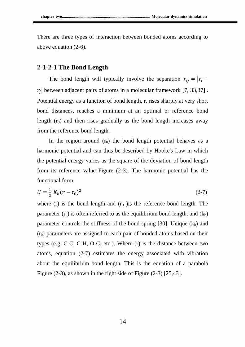
2-1-2-1 The Bond Length
The bond length will typically involve the separation |
| between adjacent pairs of atoms in a molecular framework [7, 33,37] .
Potential energy as a function of bond length, r, rises sharply at very short
bond distances, reaches a minimum at an optimal or reference bond
length (r0) and then rises gradually as the bond length increases away
from the reference bond length.
In the region around (r0) the bond length potential behaves as a
harmonic potential and can thus be described by Hooke's Law in which
the potential energy varies as the square of the deviation of bond length
from its reference value Figure (2-3). The harmonic potential has the
functional form.
( )
(2-7)
where (r) is the bond length and (r0 )is the reference bond length. The
parameter (r0) is often referred to as the equilibrium bond length, and (kb)
parameter controls the stiffness of the bond spring [30]. Unique (kb) and
(r0) parameters are assigned to each pair of bonded atoms based on their
types (e.g. C-C, C-H, O-C, etc.). Where (r) is the distance between two
atoms, equation (2-7) estimates the energy associated with vibration
about the equilibrium bond length. This is the equation of a parabola
Figure (2-3), as shown in the right side of Figure (2-3) [25,43].

chapter two ...................................................................................... Molecular dynamics simulation
04
Figure (2-3) The bond length [43].
2-1-2-2 The Bond Angles
The bond angles are between successive bond vectors such as :
and , and therefore involve three atom coordinates:
( ) ⁄
( ) ⁄
( ) (2-8)
where
. Usually this bending term is taken to be quadratic in the
angular displacement from the equilibrium value [33,7,37].
The potential energy associated with variation in bond angles(θ),
from their reference values (θ0) , is also frequently described by a
harmonic potential. The functional form of angle bending harmonic
potential is
( )
(2-9)
The description of the energetic contribution of bond angle deformation
requires two parameters: a force constant (kθ) and a reference angle (θ0)
[42].
chapter two ...................................................................................... Molecular dynamics simulation
05
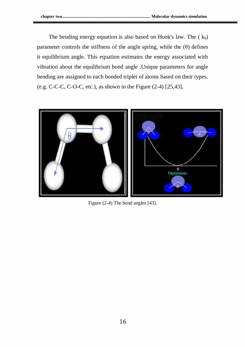
The bending energy equation is also based on Hook's law. The ( kθ)
parameter controls the stiffness of the angle spring, while the (θ) defines
it equilibrium angle. This equation estimates the energy associated with
vibration about the equilibrium bond angle .Unique parameters for angle
bending are assigned to each bonded triplet of atoms based on their types.
(e.g. C-C-C, C-O-C, etc.), as shown in the Figure (2-4) [25,43].
F
Figure (2-4) The bond angles [43].

chapter two ...................................................................................... Molecular dynamics simulation
06
2-1-2-3 The Torsion Angles
The torsion angles are defined in terms of three connected
bonds as shown in Figure (2- 5), hence four atomic coordinates:
(2-10)
and
, the unit normal to the plane defined by each pair of bonds
[33,7,37].
Intramolecular rotations (rotations about torsion or dihedral angles)
require energy (equation (2-11) and Figure (2-5)). Torsional energies are
usually important only for single bonds because double and triple bonds
are too rigid to permit rotation.
( ( )) (2-11)
The ( ) parameter controls the amplitude of the Figure (2-5-2), the
(n) parameter controls its periodicity, and ( ) is the offset or phase shift
, ( ) is torsion angle value. The parameters are determined from Figure
(2-5-2) fitting. Unique parameters for torsional rotation are assigned to
each bonded quartet of atoms based on their types (e.g. C-C-C-C, C-O-C-
N, H-C-C-H, etc.) [25, 43].
-1- -2-
Figure (2-5) The torsion angles [43].
chapter two ...................................................................................... Molecular dynamics simulation
07
2-2 The Molecular Dynamics (MD) Algorithm
The molecular dynamics algorithm have been known to Newton
equations [7,31], a system composed of atoms with coordinates
( ) and potential energy ( ), introduce the atomic momenta
( ) ,in terms of which the kinetic energy may be written
( ) ∑ | |
, then the energy (or the Hamiltonian) written
as a sum of kinetic and potential terms H = K + U. Write the classical
equations of motion as
and (2-12)
This is a system of coupled ordinary differential equations. Many
methods exist to perform step-by-step numerical integration of them.
Characteristics of these equations are: (a) they may be short and long
timescales, and the algorithm must cope with both; (b) calculating the
forces is expensive, typically involving a sum over pairs of atoms [7,
33,41].
The potential energy is a function of the atomic positions (3N) of all
the atoms in the system. Due to the complicated nature of this function,
there is no analytical solution to the equations of motion; they must be
solved numerically. Numerous numerical algorithms have been
developed for integrating the equations of motion.
All the integration algorithms assume the positions, velocities and
accelerations can be approximated by a Taylor series expansion:
( ) ( ) ( )
( )
( )
( ) ( )( ) (2-13)
( ) ( ) ( )
( ) (2-14)
( ) ( ) ( )
( ) (2-15)
( ) ( ) ( ) (2-16)

chapter two ...................................................................................... Molecular dynamics simulation
08
Where (r) is the position,(v) is the velocity (the first derivative with
respect to time), (a) is the acceleration (the second derivative with respect
to time).
2-2-1 The Verlet Algorithm
Verlet algorithm is derived as follows:
( ) ( ) ( )
( )( )
( )
( ) ( ) ( )
( )( )
( )
Summing these two equations, we obtain
( ) ( ) ( ) ( )( ) ( )
( ) ( ) ( ) ( )( ) ( )
The Verlet algorithm uses positions and accelerations at time t and
the positions from time (t-dt) to calculate new positions at time ( t+dt )
[39,42,43, 45]. Important features of the Verlet algorithm are:
1- It is exactly time reversible.
2- It is symplectic.
3- It is low order in time thus permitting long timesteps.
4- It requires just one force evaluation per timestep.
5- It is easy to implement [33,7].

chapter two ...................................................................................... Molecular dynamics simulation
11
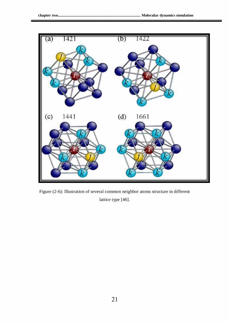
2-2-2 Common Neighbor Analysis Approach
Common neighbor analysis (CNA), first proposed by Honeycutt
and Anderson [49], is based on the analysis of common neighbors of a
pair of atoms. They introduce three properties to describe an atom pair:
0- whether they are near-neighbors.
1- the number of near neighbors they have in common.
2- the structure of these common neighbors.
According to the dislocation about common neighbor analysis
(CNA) in one parametrization using four indexes to describe the local
structure of an atom pair. In Fig. (2-6), for the pair formed by atom i and j
with blue atoms k being the common neighbors, the following indicators
i- indicates if i,j are nearest neighbors (1 = yes, 2 = no).
ii- indicates the number of common neighbors (number of k atoms).
iii- indicates the number of bonds among common neighbor atoms.
iv- indicates the bonding configuration if first three indexes are the same.
For example as (Figure 2-6), every face centered cubic ( fcc) atom has 12
pairs with index 1421 as picture (a), hexagonal close packing( hcp) atom
has 6 pairs with index 1421 and 6 pairs with index 1422 as picture b as in
Figure (2-6).
For above approach, atoms can be classified into have a local face
centered cubic (fcc), or body centered cubic (bcc), or hexagonal close
packing (hcp), or icosahedron configuration. If one atom does not belong
to any type above, the common neighbor analysis will return the value
disordered, which in most cases represents dislocation core or crack
surface. In LAMMPS, common neighbor analysis(CNA) has been
implemented by using command "compute cna/atom", the output returns
a per atom value array [46].
chapter two ...................................................................................... Molecular dynamics simulation
10
Figure (2-6): Illustration of several common neighbor atoms structure in different
lattice type [46].

chapter two ...................................................................................... Molecular dynamics simulation
11
2-2-3 Schematic of the Molecular Dynamics (MD) Algorithm
Figure (2-7) Schematic diagram of the basic MD simulation code [32]

chapter two ...................................................................................... Molecular dynamics simulation
12
2-3 Molecular Dynamics in Different Ensembles
Molecular dynamics allows use to explore the constant-energy
surface of a system. under conditions the total energy of the system is
conserved and hence different forms (i.e. ensembles) of molecular
dynamics are required. An ensemble is a collection of all possible
systems which have different microscopic states but have an identical
macroscopic or thermodynamic state. Depending on which state variables
(for example, the energy (E), volume (V), temperature (T), pressure (P),
and number of particles (N)) are kept fixed, different statistical ensembles
can be generated. A variety of structural, energetic, and dynamic
properties can then be calculated from the averages or the fluctuations of
these quantities over the ensemble generated. There exist different
ensembles with different characteristics [47].
2-3-1 Micro-Canonical or NVE Ensemble
This ensemble is characterized by a fixed number of atoms (N), a
fixed volume (V), and a fixed energy (E), is obtained by solving
Newton's standard equation of motion without any temperature and
pressure control. Energy is conserved when this ensemble is generated.
However, because of rounding and truncation errors during the
integration process, there is always a slight drift in energy. It is interested
in exploring the constant-energy surface of the conformational space. The
results can be used to calculate the thermodynamic response function

chapter two ...................................................................................... Molecular dynamics simulation
13
2-3-2 Canonical or NVT Ensemble
This ensemble is characterized by a fixed number of atoms (N), a
fixed volume (V), and a fixed temperature (T). It is also sometimes called
constant temperature molecular dynamics (CTMD). In NVT, the energy
of endothermic and exothermic processes is exchanged with a thermostat.
A variety of thermostat methods is available to add and remove energy
from the boundaries of an MD system in a more or less realistic way,
approximating the canonical ensemble.
2-3-3 Isothermal–Isobaric or NPT Ensemble
This ensemble is characterized by a fixed number of atoms (N), a
fixed pressure (P), and a fixed temperature (T). In addition to a
thermostat, a barostat is needed to control the pressure to approximate
real situation[42,47].

CHAPTER THREE
THEORETICAL part
chapter three ..................................................................................... Theoretical part
52
3-1 Quantum Many-Body Problem
In quantum mechanics the operator for the total energy is the
Hamiltonian. For a system of electrons and nuclei it can be written as
-
There are three contributions with the indices (N) for nuclei and e
for electrons. The first term in (2-1) represents the kinetic energy and the
interaction of the nucleus:
∑
∑
| |
Where
, (h) is Plank constant , is a mass of nuclei ,
( ) is the charges of the nucleus, (e) is the charge of the
electron, ( ) is radius of nucleus.
Upper case and greet subscript letters are used to indicate nuclei,
lower case and latin subscripts for electrons. The second term, , is
equivalent to the first one, except it describes electrons.
∑
∑
| |
Where (m) is mass of electron, is radius of electrons.
The third term represents the interaction between the electrons and the
nuclei:
∑∑
| |
The ground state of a non-relativistic quantum system can be
calculated with the time-independent Schrödinger equation [48],
chapter three ..................................................................................... Theoretical part
52
where the many-body wavefunction
depends on the coordinates of the (n) electrons and the (N) nuclei [48-
53]. The time evolution of the eigenstates of Eq. (3-5) is then given by
( ⁄ .
Solving the Schrödinger equation for the Hamiltonian given in Eq.
(2-1) is not possible, even for small systems containing only a few atoms
the complexity of this problem is far beyond the capabilities of any
currently available computer. For a single oxygen atom with eight
electrons the amount of data is already incredibly large. Assuming (10)
bytes are required to store a single value of the many-body wavefunction
at a discrete point in space, the storage capacity needed for the entire
function can be calculated. For a 10×10×10 grid about 1024
bytes are
needed, which could be stored on a trillion (1 TB) hard drives.
The quantum many-body problem is thus only solvable within some
approximations [48].
3-1-1 The Born-Oppenheimer Approximation
The Born-Oppenheimer is a very fundamental part of most
theoretical approaches to the quantum many-body problem. It makes use
of the fact, that the mass of the electrons is much smaller than the mass of
the nuclei. Therefore the term for the kinetic energy of the nucleus is
“small” when compared to the electron. The Born-Oppenheimer
approximation can be thought of in different ways:
1- The nuclei are decoupled from the electrons.
2- The electrons follow the motion of the nuclei a diabatically.
3- There is no exchange of energy between nuclei and electrons [48].

chapter three ..................................................................................... Theoretical part
52
As a consequence the first term in Eq. (3-2) can be neglected and the
nuclei are considered as frozen at the positions { }. The Schrödinger
equation (3-5) can then be written as
*
∑
| |
+ ∅ ∅
The wave function (∅) and the energy depend on the positions of the
nuclei only as parameters
∅ ∅ { } { }
The { } can be identified as a potential energy of the nuclei [48].
Rephrasing Eq. (3-5) yields
[ ∑
{ }
]
Where is the wave function of the nuclei. The energy (E*) is
the total energy (E) from Eq. (3-5). Using this approach, the
wavefunction (ѱ) can be separated into a part for the nuclei and a part for
the electrons:
∅ { }
Ignoring the nuclear kinetic energy, the Hamiltonian for the electrons can
then be written as
The operator for the kinetic energy of the electrons is
∑
is the potential acting on the electrons due to the nuclei,
∑
| |
chapter three ..................................................................................... Theoretical part
52
and is the electron-electron interaction,
∑
| |
The final term EII in Eq. (3-11) is the interaction of the nuclei with each
other and also includes terms that contribute to the total energy of the
system. The effect of the nuclei upon the electrons is put into an effective
external potential for the electrons, ( ) [48,49,50,52].
3-1-2 The Variational Principle
The expectation value of an operator for an eigenstate is given
by the time independent expression
⟨ ⟩ ⟨ | | ⟩
⟨ | ⟩
which involves an integral over all coordinates. For the total energy,
which is represented by the Hamiltonian from equation (3-11), this yields
⟨ | | ⟩
⟨ | ⟩ ⟨ ⟩ ⟨ ⟩ ⟨ ⟩ ∫
The expectation value of the external potential has been explicitly written
as an integral over the particle density n(r), defined as
⟨ | | ⟩
⟨ | ⟩ ∑
The nucleus-nucleus term EII is important for total energy calculations,
for the electronic structure, i.e. the wavefunctions, it is only a classical
additive term [48].
The basic task of ab initio simulation programs is finding the
eigenstates of the many-body Hamiltonian. These eigenstates are
stationary points of the energy expression Eq. (3-16). Using the
variational principle this can be expressed as :

chapter three ..................................................................................... Theoretical part
52
[⟨ | | ⟩ ⟨ | ⟩ ]
where the orthonormality of the wavefunction (⟨ | ⟩ = 1) is ensured
with a Lagrange multiplier. This is equivalent to the Rayleigh-Ritz
variation method.
The ground state wave function (Ѱ0) can thus be obtained by
minimizing the total energy with respect to all parameters in Ѱ{ri}
[48,52,54].
3-2 Density Functional Theory [55]
Density functional theory (DFT) is the most methods for
calculations (structure of atoms, molecules, crystals, surfaces and their
interactions). And also it is a ground-state theory in which the emphasis
is on the charge density as the relevant physical quantity. Density
functional theory (DFT) has been highly describing structural of most of
materials and electronic properties in a vast class of materials ranging
from atoms and molecules to simple crystals to complex extended
systems (including glasses and liquids). Furthermore density
functional theory (DFT) is computationally very simple. For these
reasons density functional theory (DFT) has become a common tool in
first-principle calculations aimed at describing or even predicting
properties of molecular and condensed matter systems.
3-2-1 Hohenberg and Kohn (H-K) Theorems
Formulation of density functional theory as an exact theory of a
many-body system. This formalism can be applied to any system of
interacting particles in an external potential , especially to
electrons and fixed nuclei, where the Hamiltonian can be written as
chapter three ..................................................................................... Theoretical part
03
∑
∑
∑
| |
The basis are the following two theorems , which can be proven very
easily [48] :
Theorem I: For any system of interacting particles in an external
potential , the potential is determined uniquely, except for a
constant, by the ground state particle density n0(r).
As a conclusion of this theorem, the Hamiltonian is fully
determined, except for a constant shift of the energy. Thus the many-body
wavefunction is also fully determined for all ground and excited states.
This means that all properties of the system are completely determined
simply be the ground state density n0(r).
Theorem II: A universal functional for the energy E[n] in terms of the
density n(r) can be defined, valid for any external potential . For
any particular , the exact ground state energy is the global
minimum value of this functional, and the density n(r) that minimizes the
functional is the exact ground state density n0(r).
This implies, that the functional E[n] is sufficient to determine the
exact ground state energy and density. This only holds for ground states,
for excited states requires additional information, such as the free-energy
functional [54-59] .
The total energy functional for a system of interacting particles is
given by
[ ] [ ] [ ] ∫
[ ] ∫
which can be derived from Eq. (3-11). The functional [ ] includes all
internal energies, potential and kinetic, of the interacting electron system,
chapter three ..................................................................................... Theoretical part
03
[ ] [ ] [ ]
The Hohenberg-Kohn theorems however are not enough to perform
electron structure calculations. An instruction on how to determine the
energy functional E[n] is required, which was given only one year
later[48,56,61,62].
3-2-2 Kohn-Sham (K-S) Equation
The Ansatz assumes that the density of the ground state of the
original interacting system is equal to that of some chosen non-interacting
system [28,29]. This leads to independent-particle equations for the non-
interacting system. They can be solved exactly with numerical methods,
the complicated many-body terms are incorporated into an exchange-
correlation functional of the density. It can be shown that the accuracy of
the results for this auxiliary system depends only on the approximation
for the exchange-correlation functional [48].
The Kohn-Sham equations are based on the total energy functional
of the Hohenberg-Kohn theorem. The ground state energy functional is
rewritten in the form
[ ] ∫ [ ] [ ]
with the independent-particle kinetic energy (TS) and the classical
Coulomb interaction energy of the electron density n(r) with itself,
[ ]
∫
| |
known as the Hartree energy.
All many-body effects of exchange and correlation in Eq. (3-23) are
grouped into the exchange-correlation energy EXC, it can be written in the
form
[ ] ⟨ ⟩ [ ] ⟨ ⟩ [ ]

chapter three ..................................................................................... Theoretical part
05
Applying the variational principle leads to the Kohn-Sham
Schrödinger-like equations:
where the are the eigenvalues and (HKS) is the effective Hamiltonian
With
If the exchange-correlation potential (VXC) were known, these
equations would lead to the exact ground state density and energy for the
interacting system. The advantage of this approach is that the remaining
functional EXC[n] can be expressed as a local or nearly local functional of
the density [48]. The long range Hartree terms and the independent
particle kinetic energies are separated out. This means that the energy EXC
can be expressed in the form
[ ] ∫ [ ]
where [ ] is an energy per electron at point (r) that depends only
upon the density n(r) in some neighborhood of point (r) [48,62-64].
3-2-3 Functionals for Exchange and Correlation
The crucial quantity in the Kohn-Sham approach is the exchange-
correlation energy, expressed as a functional of the density EXC[n] . There
are different approaches on how to choose an appropriate functional, the
two most popular being the local density approximation (LDA) and the
generalized-gradient approximation (GGA) [62].

chapter three ..................................................................................... Theoretical part
00
3-2-3-1 The Local Density Approximation (LDA)
The idea for the local density approximation (LDA) is very simple.
It was already presented by Kohn and Sham in their original publication.
Solids are often well described as a homogeneous electron gas. The
exchange-correlation energy is then simply an integral over all space
where the exchange-correlation energy density at each point is the same
as in a homogeneous electron gas with that density [48,65]
[ ] ∫
Despite of this approximation the local density approximation (LDA)
yields reasonable results for a wide range of solids. It is implemented in
most modern computer codes and has lead to improved functionals, like
generalized-gradient approximation (GGA) [48].
3-2-3-2 The Generalized Gradient Approximation (GGA)
A natural approach to improve the results of the local density
approximation (LDA) for inhomogeneous densities is the incorporation of
the gradient. The “gradient expansion approximation” (GEA) was already
proposed by Kohn and Sham in the original paper and realized by
Herman et al. in 1969. The form
[ ] ∫
however has some drawbacks. The first order derivatives often worsen
the result, while second order terms may have divergences. The basic
problem is that gradients in real materials are so large that the expansion
breaks down [48].
To deal with these problems the generalized-gradient approximation
(GGA) was developed. It splits the exchange-correlation energy density
chapter three ..................................................................................... Theoretical part
03
into the local exchange energy of the homogeneous gas and a
dimensionless gradient-dependent part (FXC),
[ ] ∫
∫
The functional form of the FXC term is rather complicated. It is usually
written as an expansion, for which the coefficients have to be determined
from training data or from mathematical constraints [48,66].
3-2-4 Pseudopotentials
One of the most expensive parts of electronic structure calculations
is the treatment of the core electrons. These tightly bound electrons have
a strongly localized wavefunction, which can vary on short distances. For
numerical calculations that is very unfavorable. To reduce the efforts
needed for the core electrons the concept of pseudopotentials was
established. The idea is to replace the strong Coulomb potential of the
nucleus and the effects of the tightly bound core electrons by an effective
ionic potential that acts on the valence electrons[48,67].
3-2-4-1 Frozen Core Approximation
The motivation for the introduction of pseudopotentials is the frozen
core approximation. It assumes that the core electrons do not participate
in chemical bonding or other electronic properties. Only the valence
electrons have an overlap with electrons from other atoms. The inner
shells can thus be treated as frozen and their wavefunctions be calculated
independently from the many-body system. This can be done either by
replacing the inner shells with an effective potential, like for most
pseudopotential methods, or by using pseudopotential operators but
chapter three ..................................................................................... Theoretical part
02
retaining the full core wavefunctions, like in the projector augmented
wave (PAW) approach [48].
3-2-4-2 Formal Justification for Pseudopotentials
A short proof for the justification of pseudopotentials, which also
gives some insight into their construction, shall be given here. It uses the
ansatz
⟩ ∅⟩ ∑ ⟩
where ⟩ is the true wavefunction, ∅⟩ the pseudo wavefunction and ⟩
are the core wavefunctions. The core and the true wavefunctions need to
be orthogonal, from which one can deduce
⟨ | ⟩ ⟨ |∅⟩ ⟨ |∅⟩
⟩ ⟩ ∑⟨ |∅⟩| ⟩
The Schrödinger equation then yields
⟩ ∅⟩ ∑ ⟩
⟨ |∅⟩ ⟩
∅⟩ ∑ ⟩
⟨ |∅⟩
⟩ ⟩
Rearranging these terms leads to
{ ∑
⟩⟨ } ∅⟩ ∅⟩
where (E) is the exact eigenvalue of the true wave function (ᴪ).Solving
this equation in a self-consistent way, the pseudo wave function as well
as the correct energy values can be obtained [48].
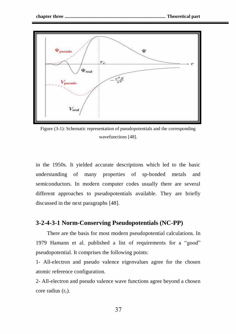
The basic idea of pseudopotentials is illustrated in Figure (3-1). For
distances smaller than a certain cutoff radius ( rc ) the real potential is
chapter three ..................................................................................... Theoretical part
02
replaced by the pseudopotential Vpseudo. The real wave function, which
has several knots in the core region, is then replaced by a pseudo wave
function without any knots. For distances greater than (rc), the all electron
wave function and the pseudo wave function are identical.
The important property, which must be conserved by the
pseudopotential, is the phase shift . The index ( ) stands for the
angular momentum of the scattered wave function and for its energy.
The scattering properties of a localized spherical potential can be
formulated in terms of this phase shift. The scattering cross-section and
all properties of the wave function outside the localized region are
determined by it.
By choosing a potential with more desirable properties, which can
reproduce the phase shift up to a modulo of( 2πn), the numerical effort
can be reduced greatly. This does not change the properties of the wave
functions outside of the scattering region, they are invariant for such
phase shifts [48].
3-2-4-3 Different Approaches for Pseudopotentials
The first ideas on how to effectively describe electron scattering
from electrons were published in the 1930 by Fermi and coworkers. A
first application of pseudopotentials to solids was presented by Hellmann
in 1935. The orthogonalized plane waves (OPWs) method of Herring was
the basis for the pseudopotential research [48].
chapter three ..................................................................................... Theoretical part
02
Figure (3-1): Schematic representation of pseudopotentials and the corresponding
wavefunctions [48].
in the 1950s. It yielded accurate descriptions which led to the basic
understanding of many properties of sp-bonded metals and
semiconductors. In modern computer codes usually there are several
different approaches to pseudopotentials available. They are briefly
discussed in the next paragraphs [48].
3-2-4-3-1 Norm-Conserving Pseudopotentials (NC-PP)
There are the basis for most modern pseudopotential calculations. In
1979 Hamann et al. published a list of requirements for a “good”
pseudopotential. It comprises the following points:
1- All-electron and pseudo valence eigenvalues agree for the chosen
atomic reference configuration.
2- All-electron and pseudo valence wave functions agree beyond a chosen
core radius (rc).

chapter three ..................................................................................... Theoretical part
02
3- The logarithmic derivatives of the all-electron and pseudo wave
functions agree at (rc).
4- The integrated charge inside (rc) for each wave function agrees (norm
conservation).
The points (1) and (2) are already clear from the definition of
pseudopotentials. Point (3) follows from the requirement of a smooth
potential, the dimensionless logarithmic derivative (D) is defined as
⁄
where ( ) is either the all-electron or pseudo wave function.
Inside of the core radius ( rc )the integrated charge ( ) has to be the
same for the all-electron (AE) and pseudo (PS) wave function [48],
∫
| |
∫
| |
This conservation ensures that the total charge in the core region is
correct and that the normalized pseudo-orbital is equal to the true orbital
outside of (rc). For solids this means, that the pseudo-orbitals are correct
between the atoms, in the region where the bonding occurs.
3-2-4-3-2 Ultrasoft Pseudopotentials (US-PP)
There are another approach to reducing the computational efforts.
Usually the goal of pseudopotentials is to have a function that is as
“smooth” as possible and yet accurate, one reason for this is that smooth
functions can be expressed with less Fourier components, which in turn
require less computational time. Increasing the “smoothness” of a
pseudopotential is equivalent to reducing the size of the Fourier space
needed to describe the valence properties with a given accuracy. For
chapter three ..................................................................................... Theoretical part
02
norm-conserving pseudopotentials this accuracy is usually reached by
sacrificing some of the “smoothness”.
The ultrasoft pseudopotentials maintain the smoothness with a
different approach. The wave function is split up into two parts, a smooth
function and an auxiliary function that represents the rapidly varying part
close to the core. In cases where most of the orbitals are tightly bound in
the core region, US-PP can yield a huge speed up compared to norm-
conserving pseudopotentials, while keeping the accuracy the same [48].
3-2-4-3-3 Projector Augmented Waves (PAW)
There are a general approach to the solution of the electronic
structure problem with the help of modern computational methods. As the
ultrasoft pseudopotentials it includes auxiliary localized functions. The
full wave function in all space can be written as
⟩ ⟩ ∑⟨ | ⟩
{ ⟩ ⟩}
where ⟩ and ⟩ are the all-electron and the smooth wave functions,
respectively. Both can be expanded into partial waves m in a sphere,
⟩ ∑ ⟩ ∑ ⟨ | ⟩ ⟩, which are the solution of the
Schrödinger equation for an isolated atom. The projection operators
are defined by ⟨ | ⟩ .
With the PAW Ansatz the full all-electron wave function is kept for the
valence part while the smoothness is also incorporated in the core region.
Especially for systems with both localized and delocalized valence states
it can be beneficial. The PAW method combines the accuracy of all-
electron methods with the efficiency of pseudopotentials. It is available in
many simulation packages[48,67].

chapter three ..................................................................................... Theoretical part
33
3-3 Embedded Atom Method (EAM)
A realistic simulation of different Semi-empirical properties of low-
symmetric metallic surfaces such as those with defects requires methods
that can simulate large numbers of atoms. Semi-empirical potentials are
good alternatives to ab-initio methods owing to their lower computational
cost. One of the early simple potentials is the two-body Lennard-Jones
(LJ) potential, which was successfully used in studying the properties of
rare gases. The first Embedded-Atom Method (EAM) potential was
proposed by Baskes and Daw [24] in 1984 on the basis of the concept of
local density, which is considered as the key variable in inter-atomic
potentials. The idea behind the EAM potential model is based on the
Quasi-atom . In the Embedded Atom Method (EAM), it is assumed that
each atom in the system is embedded in a host consisting of all the other
atoms as shown in Figure (3-2). The energy to embed an atom within the
host (embedding energy) is described as being dependent on the electron
density.
Figure 3-2. Schematic representation of the Embedded Atom Method [66].
chapter three ..................................................................................... Theoretical part
33
In the embedded atom method (EAM), the total energy of the system
is written as the addition of the embedding energy and that of the two-
body terms, as in Equation (3-41),
∑
( )
∑∅ ( )
In the former term of Equation (3-41), ) , is the sum of the
individual atomic densities ( ) as given by Equation (3-42),
∑
( )
where is the contribution of the atom( j) of type (a) to the electron
charge density at the location of the atom (I), and (Fi) is an embedding
functional that represents the energy required to place atom( i) into the
electron cloud when ( ) is the distance between atoms (i) and( j).
Therefore, the total energy of the system is a function of the atomic
positions.
In the latter term of Equation (3-41),( 𝜙 ) is the short-range pair
potential, where (Z) is the atomic number of the atoms.
∅
The total energy of the system given in Equation (3-41) has an attractive
and a repulsive part. The attractive part (first term) describes the
embedding of a positively charged core in to the electron density formed
by the surrounding atoms, while the repulsive part (second term)
describes the interactions between the ion cores [66].
To derive an approximate expression for the cohesive energy of a
metallic system that is an explicit function of the positions of the atoms
and which is simple to evaluate (i.e. equation (3-41)). This derivation has
been discussed in detail by Daw , and only summarize it here [24].

chapter three ..................................................................................... Theoretical part
35
Start with the density-functional expression for the cohesive energy
of a solid is [25].
[ ]
∑
∑
| |
∫∫
where the sums over (i) and (j) are over the nuclei of the solid, the primed
sum indicates omission of the (i =j) term, ( and ( are the charge and
position of the ith nucleus, the integrals are over [r (or r1 and r2)],
and | |. where the first term in the right side of Equation (3-
44) [ ] is the kinetic, exchange, and correlation energy
functional, [ ] [ ] [ ], where [ ] is the exchange and
correlation energy, and [ ] is the electronic kinetic energy. The second
term is the core-core repulsion potential, the third term is the electron-
core coulomb interaction, the fourth term is the electron-electron coulomb
interaction, the fifth term ( ) is the collective energy of the isolated
atoms[24,68].
Can go from equation(2-44) to equation (2-41) if make the following
two assumptions:
a): [ ]can be described by [ ] ∫
where (g) is the density and is assumed to be a function of the local
electron density and its lower derivatives.
b): the electron density of the solid can be described as a linear
superposition of the densities of the individual atoms
∑
. The first approximation is motivated by studies of the
response function of the nearly uniform electron gas. The second
approximation is justified by the observation that, in many metals, the
electron distribution in the solid is closely represented by a superposition
of atomic densities. In addition, due to the variational nature of the energy
chapter three ..................................................................................... Theoretical part
30
functional, errors in the assumed density should only affect the energy to
second order. It is also useful for to define the embedding energy for an
atom in an electron gas of some constant density (neutralized by a
positive background): ( ) [
] [
[ ]. Using these
two assumptions and the definition for the embedding energy, can obtain
from eq. (2-44):
∑ (∑
)
∑ ( )
The error ( ) is a function of the background density . Setting the
error to zero gives an equation for the optimal background density. The
solution to = 0 is discussed in detail by Daw [24].
3-4 Modified Embedded Atom Method (MEAM) [27,
25,69,70,71]
The total energy (E) of a system of atoms in the Embedded Atom
Method (EAM) has been shown to be given by an approximation of the
form:
∑(
∑∅ ( )
)
where the sums are over the atoms i and j. In this approximation, the
embedding function (Fi) is the energy to embed an atom of type (i) into
the background electron density at site i, ; and ∅ is a pair interaction
between atoms (i) and (j) whose separation is given by . In the EAM,
is given by a linear supposition of spherically averaged atomic electron
densities, while in the Modified Embedded Atom Method (MEAM), is
augmented by angularly dependent terms. Let denote the term in brackets
in Eq. (3-46), i.e., the direct contribution to the energy from the ith
atom:

chapter three ..................................................................................... Theoretical part
33
as Ei. Atom i also indirectly contributes to the energy through its
interactions with its neighbors. Then Ei may be written as follows:
∑∅ ( )
As in Baskes et al. consider the case of a homogeneous monatomic
solid with interactions limited to first neighbors only. In a specific
reference structure (usually the equilibrium structure) for an atom of type
i have:
(
)
∅
where is the background electron density for the reference
structure of atom i, Zi is the coordination, and (R) is the nearest neighbor
distance. Here is the energy per atom of the reference structure as
a function of nearest neighbor distance, obtained, e.g., from first
principles calculations or the universal equation of state of Rose et al.
Here choose the latter:
( (
)) ⁄
with
where , and B are the cohesive energy, nearest-neighbor distance,
atomic volume, and bulk modulus, respectively, all evaluated at
equilibrium in the reference state. The pair potential for like atoms is then
given by:
∅
,
( )-
At equilibrium (denoted by |re), with the use of this form, E|re =-Ec ,
dE/dr|re =0, and ⁄ |re= ⁄ so that agreement is assured

chapter three ..................................................................................... Theoretical part
32
between the model and the input cohesive energy, atomic volume, and
bulk modulus. The pair potential for unlike atom pairs will be discussed
below.
In the MEAM the embedding function F( ) is taken as
Where (A) is an adjustable parameter and is a density scaling
parameter. The density scaling parameter was initially taken to be the
coordination times the atomic density scaling factor (see Eq. 2-56 below)
and more recently as the density in the equilibrium reference structure.
The SiC calculations presented below use the latter definition. face
centered cubic (fcc), body centered cubic (bcc) reference lattices the
definitions are identical. For and hexagonal close packing (hcp) and
diamond cubic. there is a small difference.
The background electron density, , is assumed to be a function of
what call partial electron densities. These partial electron densities
contain the angular reformation in the model. The reader should be
cautioned that even though the electron density may be thought of as
qualitatively similar to a real electron density, there is no expectation that
the electron densities calculated here would be in agreement with those
obtained from first principles calculations.
For example, the square of the electron density at a given site has
previously been defined as the sum of terms with s, p, d, and f symmetry
from the neighboring atoms. By including these angular terms in the
background electron density, introduce angular forces into the model.
Thus at a particular atom:
∑

chapter three ..................................................................................... Theoretical part
32
with h=0 to 3 corresponding to s, p, d, and f symmetry, respectively, and
for convenience take . Note that in a crystal the s, p, d, and f
terms may be considered as measures of volume, polarization, shear, and
lack of inversion symmetry, respectively . For example, as vary the
volume of a perfect face centered cubic (fcc) lattice, only is not equal
to zero and, thus it can simply be related to the volume. Similarly as shear
the face centered cubic (fcc) lattice, contributions from arise. An
alternative exponential form with the same asymptotic behavior near the
perfect lattice has also been used :
* ∑ ( ⁄ )
+
The contributions to the density are given by:
∑
∑[∑
]
∑[∑
]
[∑
]
∑ [∑
]
Here, the are radial functions which represent the decrease in
the contribution with distance (r1 ) from the site in question, the
superscript (i) indicates neighboring atoms to the site in question, and
the summations are each over the three coordinate directions
with .being the distance from the site in question in that direction. The
functional forms for the partial electron densities (h=l,3) were chosen to
be translationally and rotationally invariant and equal to zero for crystals

chapter three ..................................................................................... Theoretical part
32
with cubic symmetry. Finally, the individual contributions are assumed to
decrease exponentially, i.e.,
⁄
where and are constants. For alloys the coefficients t
(h) were
initially assumed to depend on the properties of the atom at which the
average electron density was calculated. agreement with defect properties
in SiC could be obtained if the properties of the atoms surrounding this
atom were included. The latter averaging procedure is used below for the
SiC calculations:
∑
⁄
3-5 Molecular Dynamics (MD) Modeling of Fracture
3-5-1 Model Potentials for Brittle Materials
The most critical input parameter in Molecular Dynamics (MD) is
the choice of interatomic potentials, it is difficult to identify generic
relationships between potential parameters and macroscopic observables
such as the crack limiting or instability speeds when using such
complicated potentials. Deliberately avoid these complexities by adopting
a simple pair potential based on a harmonic interatomic potential with
spring constant ( k ) [72]. In this case, the interatomic potential between
pairs of atoms is expressed as
∅
where ( ) denotes the equilibrium distance between atoms, for a two
dimensions (2D) triangular lattice, as schematically shown in the inlay of
Fig. (3-3). This harmonic potential is a first-order approximation of the
Lennard-Jones potential , one of the simplest and most widely used pair
potentials defined as

chapter three ..................................................................................... Theoretical part
32
∅ (*
+
*
+
)
Express all quantities in reduced units, so that lengths are scaled by
the LJ-parameter (σ) which is assumed to be unity, and energies are
scaled by the parameter (ε) , the depth of the minimum of the LJ
potential. Corresponding to choosing ε = 1 in Eq. (3-59), choose (a0 = −1)
in the harmonic approximation shown in Eq. (3-58). Further, more
√
(see Fig. (3-3)). The parameter (σ) is coupled to
the lattice constant (a) as √
√ ⁄⁄ . The reduced temperature is
⁄ with being the Boltzmann constant. The mass of each
atoms in the models is assumed to be unity, relative to the reference mass
( m*) . The reference time unit is then given by √ ⁄ . For
example, when choosing electron volt as reference energy (ε = 1eV),
Angstrom as reference length (σ = 1 Å), and the atomic mass unit as
reference mass (m* = 1 amu), the reference time unit corresponds to (t* ≈
1.01805E-14 seconds) [72].
Although the choice of a simple harmonic interatomic potential can
not lead to quantitative calculations of fracture properties in a particular
material, it allows to draw certain generic conclusions about fundamental,
material-independent mechanisms that can help elucidating the physical
foundations of brittle fracture. The harmonic potential leads to linear
elastic material properties, and thus serves as the starting point when
comparing simulation results to predictions by the classical linear theories
of fracture.
In Fig (3-3), (a) the geometry is characterized by the slab width lx
and slab length ly , and the initial crack length a. Consider different
loading cases, including mode I, mode II (indicated in the figure) and
mode III (not shown). Subplots (b) and (c) illustrate two different

chapter three ..................................................................................... Theoretical part
32
possible crack orientations. The orientation shown in subplot (c) has
lower fracture surface energy than the orientation shown in subplot (b)
[72].
Figure 3-3. A schematic illustration of the simulation geometry used in our large-
scale atomistic studies of fracture [72].
chapter three ..................................................................................... Theoretical part
23
3-5-2 Model Geometry and Simulation Procedure
A crack in a two-dimensional geometry with slab size (lx × ly) and
initial crack length (a), as schematically shown in Fig. (3-3). The slab
size is chosen large enough such that waves reflected from the boundary
do not interfere with the propagating crack at early stages of the
simulation. The slab size in the crack direction is chosen between 2 and 4
times larger than the size orthogonal to the initial crack. The slab is
initialized at zero temperature prior to simulation. Most of studies are
carried out in a two-dimensional, hexagonal lattice. The three-
dimensional studies are performed in a face centered cubic (FCC) lattice,
with periodic boundary conditions in the out-of-plane in Z-direction [72].

CHAPTER FOUR
RESULTS AND
DISCUSSION

chapter four ........................................................................... Results & Discussions
15
4-1 Crack code
Dynamic fracture is investigated for two-dimensional notched solids
under tension using million atom systems [74]. The material which test in
this code is brittle material with hexagonal style in two dimension (2d)
lattice, the unit cell is rectangular, with miller indices a1 = [1 0 0] and a2 =
[0 sqrt(3) 0]. In crack used time step (0.044.0.04,0.03, 0.02, 0.01, 0.009,
0.008, 0.007, 0.006, 0.005, 0.004, 0.003, 0.002, 0.001and 0.00001 tau
( √ ⁄ ) as shown in Table (4-1). The output obtained from
Large-scale Atomic/Molecular Massively Parallel Simulator (LAMMPS)
is used to calculate various values such as temperature, total energy,
kinetic energy, potential energy, pressure and volume. Statistica used to
plot graphs. After implementation of the simulation program the results
of crack code shown in the table (4-1) and table (4-2).
The total energy in each time step (E = K(t)+U(t)) is conserved by
Newtonian dynamics. Moving each atom in a time in separate steps
known as time-steps, run command continues dynamics for a specified
number of time steps [74]. Time step command sets time step size ( )
for molecular dynamics simulations [67] , time step exist in the Euler
equation and other equations according to the equation (2-14). We choose
time step small to minimize the error and these idea is consistent with
[77] where they chose time step small enough to ensure energy
conservation and avoid large discretization errors. The step (run)
evolution of the total energy as shown in Figure (4-5) and Table (4-1),
where the (0.044, 0.04, 0.03, 0.03, 0.01 tau ( √ ⁄ ) time step )
the input data in appendix I( gives increased then rise to small oscillations
in total energy, furthermore, the (0.001,0.002, 0.003, 0.004, 0.005, 0.006,
0.007, 0.008, 0.009 tau ( √ ⁄ ) time step where increasing the

chapter four ........................................................................... Results & Discussions
12
total energy and this is violates energy conservation, a time step of
(0.00001 tau ( √ ⁄ ) has therefore been to be the optimum
choice, balancing energy conservation.

chapter four ........................................................................... Results & Discussions
15
0.0
00
01
Tota
l en
ergi
es (
epsi
lon
)
-3.1
92
51
-3.1
92
51
-3.1
92
51
-3.1
92
51
-3.1
92
51
-3.1
92
5
-3.1
92
5
-3.1
92
5
-3.1
92
5
-3.1
92
5
-3.1
92
5 -3
.19
24
9
-3.1
92
49
-3.1
92
49
-3.1
92
49
-3.1
92
49
-3.1
92
48
-3.1
92
48
-3.1
92
48
-3.1
92
48
-3.1
92
49
-3.1
92
48
-3.1
92
47
-3.1
92
47
-3.1
92
47
-3.1
92
47
0.0
01
-3.1
92
51
--3
.19
23
1
-3.1
91
93
-3.1
91
32
-3.1
90
62
-3.1
89
75
-3.1
88
68
-3.1
87
34
-3.1
85
77
-3.1
84
09
-3.1
82
21
-3.1
80
11
-3.1
77
92
-3.1
75
68
-3.1
73
41
-3.1
70
85
-3.1
68
09
-3.1
65
25
-3.1
62
3
-3.1
59
17
-3.1
56
06
-3.1
52
76
-3.1
49
25
-3.1
45
73
-3.1
42
1
-3.1
38
61
0.0
02
-3.1
92
51
-3.1
91
93
-3.1
90
62
-3.1
88
68
-3.1
85
77
-3.1
82
21
-3.1
77
92
-3.1
73
41
-3.1
68
09
-3.1
62
3
-3.1
56
06
-3.1
49
25
-3.1
42
1
-3.1
35
04
-3.1
27
49
-3.1
19
9
-3.1
11
86
-3.1
03
66
-3.0
95
22
-3.0
86
65
-3.0
77
91
-3.0
69
22
-3.0
60
34
-3.0
51
37
-3.0
42
29
-3.0
33
34
0.0
03
-3.1
91
32
-3.1
91
32
-3.1
88
68
-3.1
84
09
-3.1
77
92
-3.1
70
85
-3.1
62
3
-3.1
52
75
-3.1
42
1
-3.1
31
27
-3.1
19
9
-3.1
07
79
-3.0
95
22
-3.0
82
31
-3.0
69
22
-3.0
55
83
-3.0
42
29
-3.0
28
75
-3.0
15
29
-3.0
01
67
-2.9
89
57
-2.9
80
61
-2.9
69
48
-2.9
56
76
-2.9
44
13
-2.9
40
11
0.0
04
-3.1
92
51
-3.1
90
62
-3.1
85
77
-3.1
77
92
-3.1
68
09
-3.1
56
05
-3.1
42
09
-3.1
27
49
-3.1
11
86
-3.0
95
22
-3.0
77
91
-3.0
60
33
-3.0
42
29
-3.0
24
27
-3.0
06
1
-2.9
89
56
-2.9
77
28
-2.9
61
12
-2.9
44
12
-2.9
29
21
-2.9
15
86
-2.9
03
45
-2.8
95
32
-2.8
89
74
-2.8
85
44
-2.8
78
74
0.0
05
-3.1
92
51
-3.1
89
75
-3.1
82
21
-3.1
70
85
-3.1
56
05
-3.1
38
6
-3.1
19
9
-3.0
99
46
-3.0
77
91
-3.0
55
83
-3.0
33
34
-3.0
10
67
-2.9
89
56
-2.9
73
56
-2.9
52
51
-2.9
32
3
-2.9
15
93
-2.9
00
63
-2.8
92
55
-2.8
86
64
-2.8
79
26
-2.8
69
08
-2.8
61
1
-2.8
56
29
-2.8
48
94
-2.8
43
67
0.0
06
-3.1
92
51
-3.1
88
67
-3.1
77
91
-3.1
62
29
-3.1
42
09
-3.1
19
9
-3.0
95
21
-3.0
69
22
-3.0
42
28
-3.0
15
28
-2.9
89
55
-2.9
69
5
-2.9
44
13
-2.9
22
68
-2.9
03
36
-2.8
92
56
-2.8
85
85
-2.8
74
64
-2.8
64
34
-2.8
57
63
-2.8
49
62
-2.8
42
69
-2.8
35
34
-2.8
32
16
-2.8
28
5
-2.8
24
4
0.0
07
-3.1
92
51
-3.1
87
33
-3.1
73
4
-3.1
52
75
-3.1
27
48
-3.0
99
46
-3.0
69
22
-3.0
37
85
-3.0
06
09
-2.9
80
62
-2.9
52
48
-2.9
25
98
-2.9
03
51
-2.8
90
96
-2.8
82
52
-2.8
69
56
-2.8
60
52
-2.8
52
96
-2.8
44
98
-2.8
36
69
-2.8
33
47
-2.8
28
99
-2.8
24
64
-2.8
25
45
-2.8
23
12
-2.8
20
63
0.0
08
-3.1
92
51
-3.1
85
76
-3.1
68
08
-3.1
42
08
-3.1
11
85
-3.0
77
9
-3.0
42
28
-3.0
06
09
-2.9
77
29
-2.9
44
1
-2.9
15
99
-2.8
95
12
-2.8
85
36
-2.8
52
2
-2.8
58
8
-2.8
49
57
-2.8
39
35
-2.8
32
33
-2.8
27
82
-2.8
23
02
-2.8
18
94
-2.8
17
21
-2.8
13
51
-2.8
08
58
-2.8
03
99
-2.8
01
45
0.0
09
-3.1
92
51
-3.1
84
07
-3.1
62
28
-3.1
31
26
-3.0
95
21
-3.0
55
84
-3.0
15
27
-2.9
80
61
-2.9
44
09
-2.9
13
08
-2.8
92
57
-2.8
79
44
-2.8
62
29
-2.8
52
2
-2.8
43
22
-2.8
32
39
-2.8
32
39
-2.8
28
98
-2.8
26
65
-2.8
22
97
-2.8
16
01
-2.8
13
83
-2.8
07
9
-2.8
04
89
-2.7
98
22
-2.7
91
92
0.0
1
-3.1
92
51
-3.1
82
19
-3.1
56
04
-3.1
19
89
-3.0
77
89
-3.0
33
33
-2.9
89
54
-2.9
52
49
-2.9
16
-2.8
92
56
-2.8
78
68
-2.8
61
64
-2.8
50
34
-2.8
40
61
-2.8
31
81
-2.8
29
54
-2.8
27
74
-2.8
24
79
-2.8
18
48
-2.8
14
16
-2.8
09
21
-2.8
04
86
-2.7
98
03
-2.7
94
28
-2.7
90
44
-2.7
88
8
0.0
2
-3.1
92
51
-3.1
55
99
-3.0
77
83
2.9
89
43
-2.9
15
38
-2.8
75
83
-2.8
42
27
-2.8
21
71
-2.8
19
29
-2.8
18
17
-2.8
02
91
-2.7
93
83
-2.7
90
71
-2.7
86
8
-2.7
80
82
-2.7
77
56
-2.7
77
03
-2.7
82
21
-2.7
83
64
-2.7
81
46
-2.7
78
49
-2.7
78
79
-2.7
83
76
-2.7
82
57
-2.7
79
87
-2.7
81
04
0.0
3
-3.1
92
51
-3.1
19
74
-2.9
89
22
-2.8
89
5
-2.8
46
75
-2.8
30
26
-2.8
20
21
-2.8
21
71
2.7
95
67
-2.7
93
24
2.7
85
32
-2.7
75
92
-2.7
79
24
-2.7
74
92
-2.7
66
64
-2.7
65
3
-2.7
66
25
-2.7
64
09
-2.7
60
41
-2.7
69
88
-2.7
70
52
-2.7
63
6
-2.7
68
95
2.7
68
96
-2.7
65
17
-2.7
66
83
0.0
4
-3.1
92
51
-3.0
77
58
-2.9
14
19
-2.8
35
14
-2.8
26
15
-2.7
92
08
-2.7
75
96
-2.7
72
1
-2.7
62
09
-2.7
53
68
-2.7
56
39
-2.7
43
62
-2.7
51
76
-2.7
46
61
-2.7
47
51
-2.7
60
75
-2.7
45
42
-2.7
54
43
-2.7
52
41
-2.7
49
21
-2.7
55
6
-2.7
46
97
-2.7
50
14
-2.7
52
41
-2.7
50
3
-2.7
49
16
0.0
44
-3.1
92
51
-3.0
59
98
-2.8
90
18
-2.8
37
33
-2.8
26
15
-2.7
95
2
-2.7
89
09
-2.7
85
04
-2.7
75
68
-2.7
82
08
-2.7
68
29
-2.7
76
31
-2.7
64
39
-2.7
68
01
-2.7
61
63
-2.7
63
13
-2.7
60
72
-2.7
55
67
-2.7
55
3
-2.7
48
6
-2.7
51
79
-2.7
38
43
-2.7
40
14
-2.7
33
68
-2.7
29
77
-2.7
26
38
Tim
e
ste
p
Step
)ru
n)
0
20
0
40
0
60
0
80
0
10
00
12
00
14
00
16
00
18
00
20
00
22
00
24
00
26
00
28
00
30
00
32
00
34
00
36
00
38
00
40
00
42
00
44
00
46
00
48
00
50
00
Tab
le 4
-1:
To
tal
ener
gy
vs.
ste
p (
run)
at r
un=
500
0 i
n c
rack
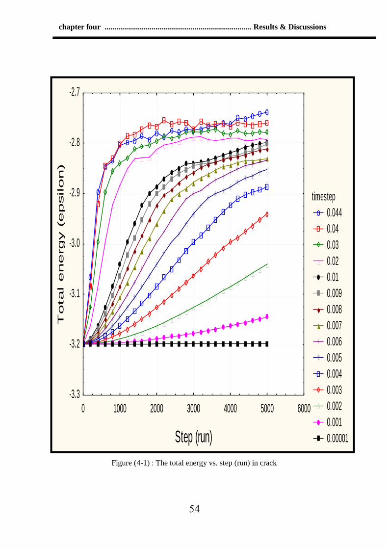
chapter four ........................................................................... Results & Discussions
14
Figure (4-1) : The total energy vs. step (run) in crack
timestep
0.044
0.04
0.03
0.02
0.01
0.009
0.008
0.007
0.006
0.005
0.004
0.003
0.002
0.001
0.00001
0 1000 2000 3000 4000 5000 6000
Step (run)
-3.3
-3.2
-3.1
-3.0
-2.9
-2.8
-2.7
Total energy (epsilon)

chapter four ........................................................................... Results & Discussions
11
In molecular mechanics atoms movement based on their potential
energy instead of the calculated force. Energy minimization is a way to
relax the system before any runs by finding a stable equilibrium for that
system, energy minimization can also be used to find the most stable state
of molecules, If the simulation box contains 3200 atoms, then potential
would be calculated 3199 times for each atom per time step, an atom-
atom distance calculated, and computing the Lennard-Jones potential
gives a total of more than 20 million calculations. If any atom is closer to
target atom than this distance, then can proceed with calculating the
potential. If the atom-atom distance is larger than the cutoff, then the
potential calculation is ignored. This cuts the number of calculations
roughly in half. LAMMPS does not support these functions and simply
set the potentials to zero for distances above cutoff [73].
The potential energy in crack is its Lennard-Jones potential (non-
bonded), the potential energy is negative because of negative cohesive
energy, in energy versus distance between two atoms plot in LJ (
Lennard-Jones) type of potential , see a drop in energy at the equilibrium
position of two atoms.
At the atomic level, when an external load is applied to a material
the atoms are displaced from their original equilibrium position straining
their bonds. In order for a bond to be severed and an atom to be
permanently displaced from its equilibrium position, the external load on
the material must translate to an acting atomic level force that is greater
than the cohesive force binding the atoms. Additionally, this force must
perform a minimum amount of work equal to the bond energy. The
equilibrium atomic separation or bond length occurs at the minimum of
the potential energy where the force is zero. The magnitude of the force
(slope of the potential) on the atoms is shown for distances beyond
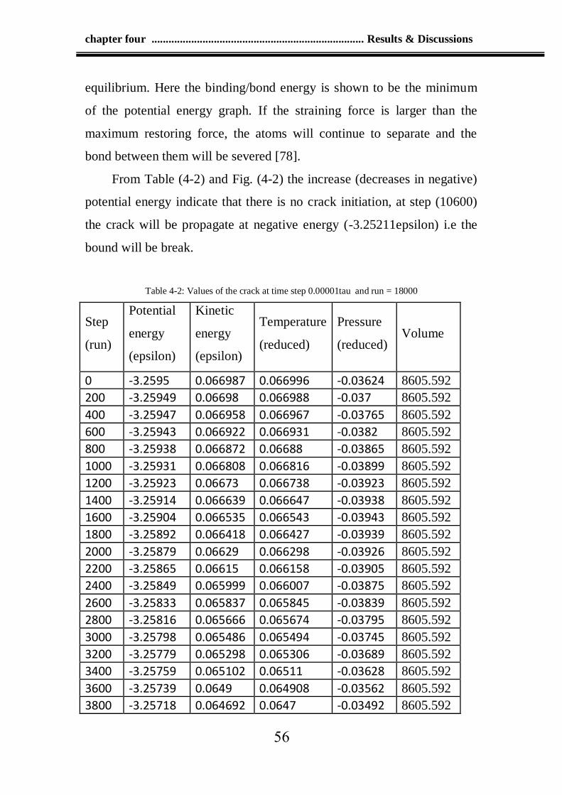
chapter four ........................................................................... Results & Discussions
17
equilibrium. Here the binding/bond energy is shown to be the minimum
of the potential energy graph. If the straining force is larger than the
maximum restoring force, the atoms will continue to separate and the
bond between them will be severed [78].
From Table (4-2) and Fig. (4-2) the increase (decreases in negative)
potential energy indicate that there is no crack initiation, at step (10600)
the crack will be propagate at negative energy (-3.25211epsilon) i.e the
bound will be break.
Table 4-2: Values of the crack at time step 0.00001tau and run = 18000
Volume Pressure
(reduced)
Temperature
(reduced)
Kinetic
energy
(epsilon)
Potential
energy
(epsilon)
Step
(run)
8605.592 -0.03624 0.066996 0.066987 -3.2595 0
8605.592 -0.037 0.066988 0.06698 -3.25949 200
8605.592 -0.03765 0.066967 0.066958 -3.25947 400
8605.592 -0.0382 0.066931 0.066922 -3.25943 600
8605.592 -0.03865 0.06688 0.066872 -3.25938 800
8605.592 -0.03899 0.066816 0.066808 -3.25931 1000
8605.592 -0.03923 0.066738 0.06673 -3.25923 1200
8605.592 -0.03938 0.066647 0.066639 -3.25914 1400
8605.592 -0.03943 0.066543 0.066535 -3.25904 1600
8605.592 -0.03939 0.066427 0.066418 -3.25892 1800
8605.592 -0.03926 0.066298 0.06629 -3.25879 2000
8605.592 -0.03905 0.066158 0.06615 -3.25865 2200
8605.592 -0.03875 0.066007 0.065999 -3.25849 2400
8605.592 -0.03839 0.065845 0.065837 -3.25833 2600
8605.592 -0.03795 0.065674 0.065666 -3.25816 2800
8605.592 -0.03745 0.065494 0.065486 -3.25798 3000
8605.592 -0.03689 0.065306 0.065298 -3.25779 3200
8605.592 -0.03628 0.06511 0.065102 -3.25759 3400
8605.592 -0.03562 0.064908 0.0649 -3.25739 3600
8605.592 -0.03492 0.0647 0.064692 -3.25718 3800
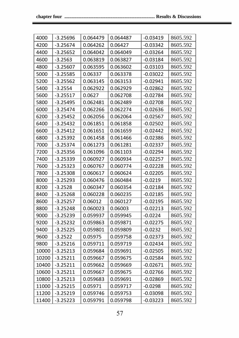
chapter four ........................................................................... Results & Discussions
16
8605.592 -0.03419 0.064487 0.064479 -3.25696 4000
8605.592 -0.03342 0.06427 0.064262 -3.25674 4200
8605.592 -0.03264 0.064049 0.064042 -3.25652 4400
8605.592 -0.03184 0.063827 0.063819 -3.2563 4600
8605.592 -0.03103 0.063602 0.063595 -3.25607 4800
8605.592 -0.03022 0.063378 0.06337 -3.25585 5000
8605.592 -0.02941 0.063153 0.063145 -3.25562 5200
8605.592 -0.02862 0.062929 0.062922 -3.2554 5400
8605.592 -0.02784 0.062708 0.0627 -3.25517 5600
8605.592 -0.02708 0.062489 0.062481 -3.25495 5800
8605.592 -0.02636 0.062274 0.062266 -3.25474 6000
8605.592 -0.02567 0.062064 0.062056 -3.25452 6200
8605.592 -0.02502 0.061858 0.061851 -3.25432 6400
8605.592 -0.02442 0.061659 0.061651 -3.25412 6600
8605.592 -0.02386 0.061466 0.061458 -3.25392 6800
8605.592 -0.02337 0.061281 0.061273 -3.25374 7000
8605.592 -0.02294 0.061103 0.061096 -3.25356 7200
8605.592 -0.02257 0.060934 0.060927 -3.25339 7400
8605.592 -0.02228 0.060774 0.060767 -3.25323 7600
8605.592 -0.02205 0.060624 0.060617 -3.25308 7800
8605.592 -0.0219 0.060484 0.060476 -3.25293 8000
8605.592 -0.02184 0.060354 0.060347 -3.2528 8200
8605.592 -0.02185 0.060235 0.060228 -3.25268 8400
8605.592 -0.02195 0.060127 0.06012 -3.25257 8600
8605.592 -0.02213 0.06003 0.060023 -3.25248 8800
8605.592 -0.0224 0.059945 0.059937 -3.25239 9000
8605.592 -0.02275 0.059871 0.059863 -3.25232 9200
8605.592 -0.0232 0.059809 0.059801 -3.25225 9400
8605.592 -0.02373 0.059758 0.05975 -3.2522 9600
8605.592 -0.02434 0.059719 0.059711 -3.25216 9800
8605.592 -0.02505 0.059691 0.059684 -3.25213 10000
8605.592 -0.02584 0.059675 0.059667 -3.25211 10200
8605.592 -0.02671 0.059669 0.059662 -3.25211 10400
8605.592 -0.02766 0.059675 0.059667 -3.25211 10600
8605.592 -0.02869 0.059691 0.059683 -3.25213 10800
8605.592 -0.0298 0.059717 0.05971 -3.25215 11000
8605.592 -0.03098 0.059753 0.059746 -3.25219 11200
8605.592 -0.03223 0.059798 0.059791 -3.25223 11400
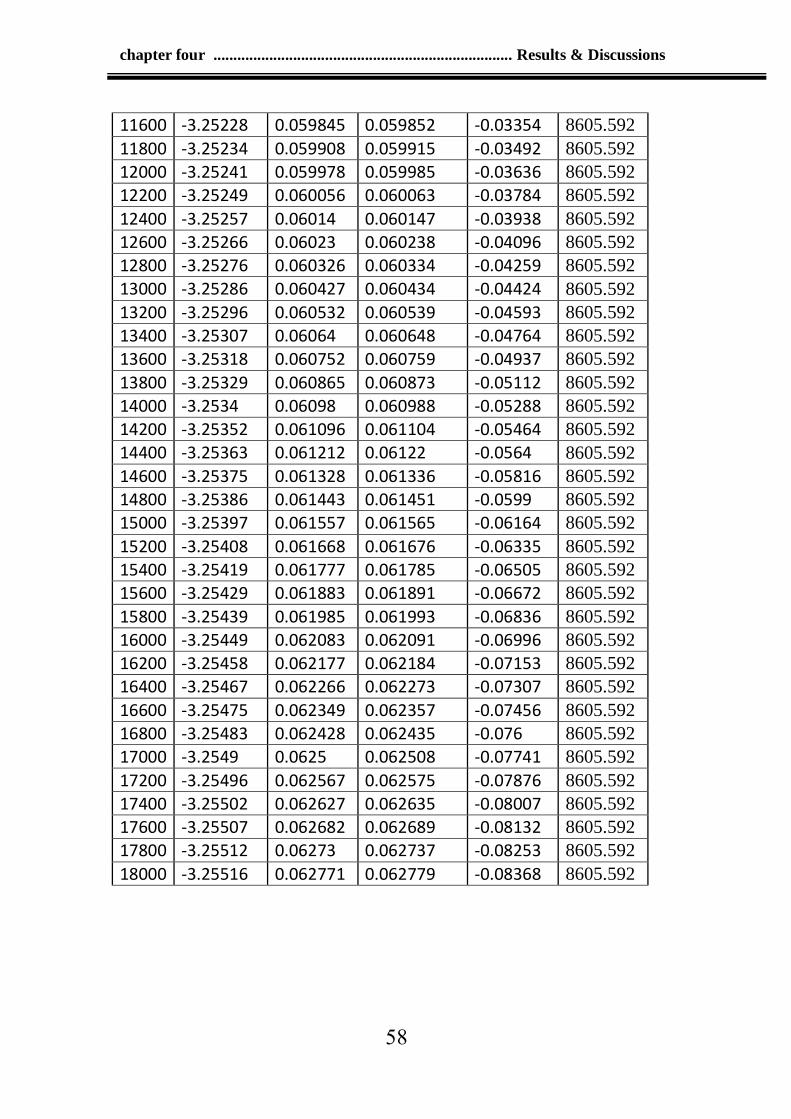
chapter four ........................................................................... Results & Discussions
15
8605.592 -0.03354 0.059852 0.059845 -3.25228 11600
8605.592 -0.03492 0.059915 0.059908 -3.25234 11800
8605.592 -0.03636 0.059985 0.059978 -3.25241 12000
8605.592 -0.03784 0.060063 0.060056 -3.25249 12200
8605.592 -0.03938 0.060147 0.06014 -3.25257 12400
8605.592 -0.04096 0.060238 0.06023 -3.25266 12600
8605.592 -0.04259 0.060334 0.060326 -3.25276 12800
8605.592 -0.04424 0.060434 0.060427 -3.25286 13000
8605.592 -0.04593 0.060539 0.060532 -3.25296 13200
8605.592 -0.04764 0.060648 0.06064 -3.25307 13400
8605.592 -0.04937 0.060759 0.060752 -3.25318 13600
8605.592 -0.05112 0.060873 0.060865 -3.25329 13800
8605.592 -0.05288 0.060988 0.06098 -3.2534 14000
8605.592 -0.05464 0.061104 0.061096 -3.25352 14200
8605.592 -0.0564 0.06122 0.061212 -3.25363 14400
8605.592 -0.05816 0.061336 0.061328 -3.25375 14600
8605.592 -0.0599 0.061451 0.061443 -3.25386 14800
8605.592 -0.06164 0.061565 0.061557 -3.25397 15000
8605.592 -0.06335 0.061676 0.061668 -3.25408 15200
8605.592 -0.06505 0.061785 0.061777 -3.25419 15400
8605.592 -0.06672 0.061891 0.061883 -3.25429 15600
8605.592 -0.06836 0.061993 0.061985 -3.25439 15800
8605.592 -0.06996 0.062091 0.062083 -3.25449 16000
8605.592 -0.07153 0.062184 0.062177 -3.25458 16200
8605.592 -0.07307 0.062273 0.062266 -3.25467 16400
8605.592 -0.07456 0.062357 0.062349 -3.25475 16600
8605.592 -0.076 0.062435 0.062428 -3.25483 16800
8605.592 -0.07741 0.062508 0.0625 -3.2549 17000
8605.592 -0.07876 0.062575 0.062567 -3.25496 17200
8605.592 -0.08007 0.062635 0.062627 -3.25502 17400
8605.592 -0.08132 0.062689 0.062682 -3.25507 17600
8605.592 -0.08253 0.062737 0.06273 -3.25512 17800
8605.592 -0.08368 0.062779 0.062771 -3.25516 18000
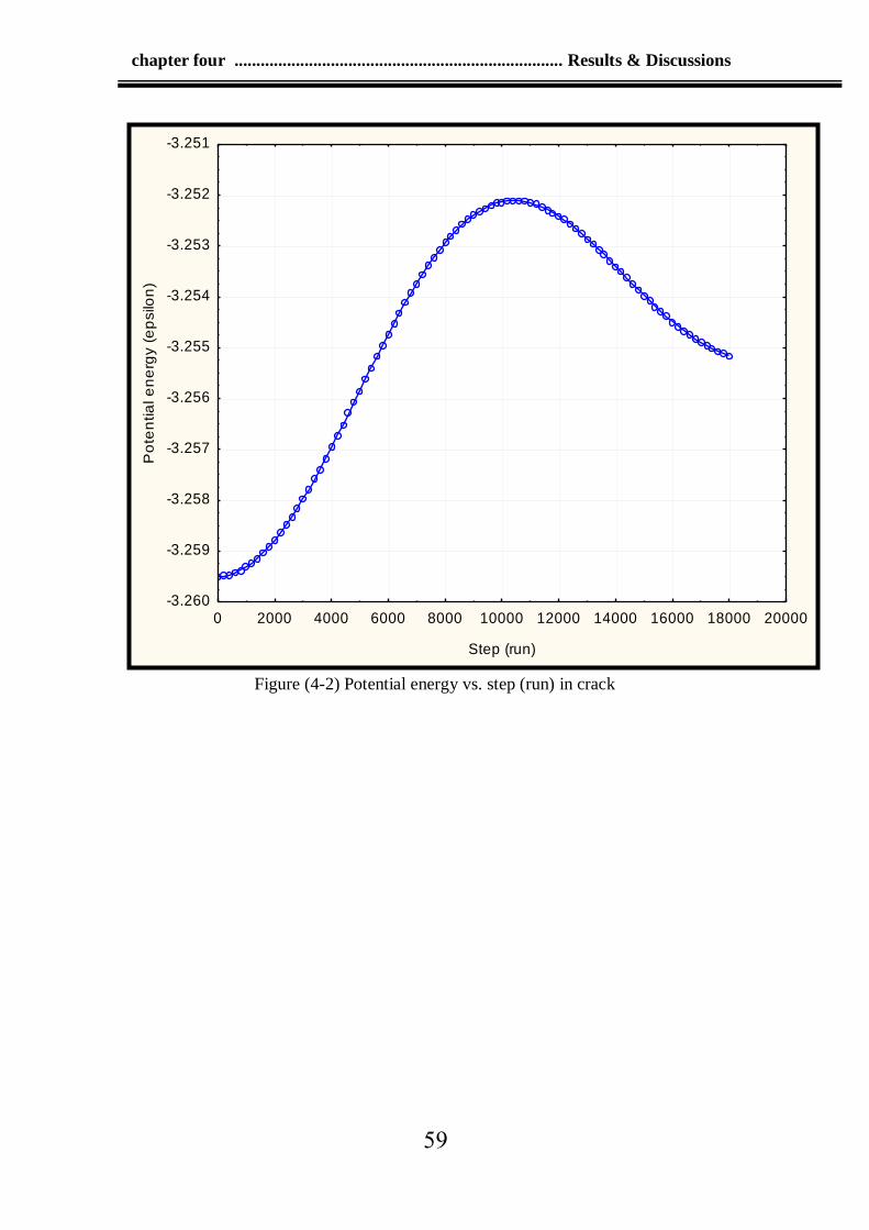
chapter four ........................................................................... Results & Discussions
15
0 2000 4000 6000 8000 10000 12000 14000 16000 18000 20000
Step (run)
-3.260
-3.259
-3.258
-3.257
-3.256
-3.255
-3.254
-3.253
-3.252
-3.251P
ote
ntia
l e
ne
rgy (
ep
silo
n)
Figure (4-2) Potential energy vs. step (run) in crack

chapter four ........................................................................... Results & Discussions
76
0 2000 4000 6000 8000 10000 12000 14000 16000 18000 20000
Step (run)
0.059
0.060
0.061
0.062
0.063
0.064
0.065
0.066
0.067
0.068
Kin
etic e
ne
rgy (
ep
silo
n)
From Fig. (4-3) and Table (4-2), the decreases in kinetic energy lead
to reduce the speed of the atoms because there is no crack initiation, the
increases of kinetic energy (0.059667) at step (run) =10600, it is obvious
that the rapid breaking of local atomic bonds in brittle fracture gives rise
to a higher atomic kinetic energy at the crack tip [74].
Figure (4-3) Kinetic energy vs. step (run) in crack

chapter four ........................................................................... Results & Discussions
75
0 2000 4000 6000 8000 10000 12000 14000 16000 18000 20000
Step (run)
0.059
0.060
0.061
0.062
0.063
0.064
0.065
0.066
0.067
0.068
Te
mp
era
ture
(re
du
ce
d)
The conversion of energy from potential energy to kinetic energy in
a closed system raises the system temperature [78]. Temperature units is
reduced (
) . decrease in temperature because there is no crack
initiation, the increase in temperature indicates that the crack propagated
as shown in Fig. (4-4) and Table (4-2).
Figure (4-4) Temperature vs. step (run) in crack

chapter four ........................................................................... Results & Discussions
72
0 2000 4000 6000 8000 10000 12000 14000 16000 18000 20000
Step (run)
-0.09
-0.08
-0.07
-0.06
-0.05
-0.04
-0.03
-0.02
-0.01
Pre
ssu
re (
red
uce
d)
pressure is external force per unit area. It is the force distribution
normal to the surface . pressure unite is reduced (
).
From Fig. (4-5) and Table (4-2) , decreases in negative pressure
because there is no crack initiation, the increase in negative pressure
resulting from breaking the bonds between atoms.
Figure (4-5) Pressure vs. step (run) in crack
chapter four ........................................................................... Results & Discussions
75
0 2000 4000 6000 8000 10000 12000 14000 16000 18000 20000
Step (run)
8603
8604
8605
8606
8607
8608
Vo
lum
e (
sig
ma
)In this thesis used NVE microcanonical ensemble simulations, so
the volume or area of crack is constant as shown in Fig. (4-6) and Table
(4-2).
Figure (4-6) Volume vs. step (run) in crack

chapter four ........................................................................... Results & Discussions
74
4-2 Modified Embedded Atom Method (MEAM) code
After the implementation of the simulation program the results of
Modified Embedded Atom Method (MEAM) code as shown in the tables
(4-3) and (4-4) . The total energy in each time step (E = K(t)+U(t)) is
conserved by Newtonian dynamics.
the time step must be chosen small enough to ensure energy
conservation and avoid large discretization errors [77]. From Fig (4-7)
and Table (4-3) shows the response of total energy vs. run time for time
step (0.0001 Ps) is stable at value (-636.4) while for (0.0005, 0.0006,
0.0007, 0.0008, 0.0009 and 0.001 Ps) the total energy decrease and then
be stable for (0.002, 0.003 Ps) the total energy be unstable this means that
the stable time step for numerical solution for Modified Embedded Atom
Method (MEAM) equation so used time step (0.0001 Ps) for calculation.
Table 4-3 : Total energy vs. step (run) in MEAM
0.0001 0.0005 0.0006 0.0007 0.0008 0.0009 0.001 0.002 0.003 Time
step
(Ps)
Step
(run) Total energies (eV)
-636.381 -636.381 -636.381 -636.381 -636.381 -636.381 -636.381 -636.381 -636.381 0
-636.381 -636.433 -636.456 -636.475 -636.494 -636.516 -636.541 -637.009 -637.886 10
-636.382 -636.421 -636.441 -636.462 -636.478 -636.502 -636.535 -637.106 -637.452 20
-636.383 -636.421 -636.435 -636.458 -636.485 -636.535 -636.548 -637.047 -637.497 30
-636.383 -636.42 -636.439 -636.466 -636.483 -636.519 -636.562 -636.949 -637.079 40
-636.383 -636.423 -636.442 -636.461 -636.499 -636.507 -636.565 -636.981 -637.142 50
-636.383 -636.422 -636.442 -636.47 -636.488 -636.509 -636.55 -636.999 -637.098 60
-636.383 -636.421 -636.448 -636.465 -636.482 -636.518 -636.542 -636.945 -637.293 70
-636.383 -636.425 -636.441 -636.455 -636.485 -636.477 -636.536 -637.121 -637.325 80
-636.383 -636.418 -636.437 -636.462 -636.457 -636.493 -636.523 -637.033 -637.34 90
-636.383 -636.426 -636.441 -636.459 -636.482 -636.497 -636.531 -637.025 -637.479 100
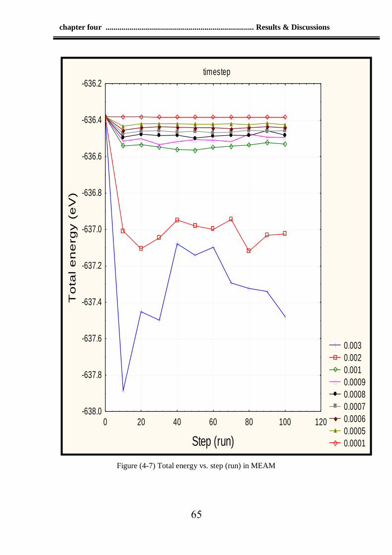
chapter four ........................................................................... Results & Discussions
71
timestep
0.003
0.002
0.001
0.0009
0.0008
0.0007
0.0006
0.0005
0.0001
0 20 40 60 80 100 120
Step (run)
-638.0
-637.8
-637.6
-637.4
-637.2
-637.0
-636.8
-636.6
-636.4
-636.2
To
tal e
ne
rg
y (
eV
)
Figure (4-7) Total energy vs. step (run) in MEAM

chapter four ........................................................................... Results & Discussions
77
Complex chemical bonds in SiC involve both ionic and covalent
characters. There is charge transfer between Si and C atoms resulting in
Coulomb interaction between ions, so the two-body interaction potential
must contain at a minimum a steric repulsion as well as Coulomb
interaction [18]. Potential energy in Modified Embedded Atom Method
code (MEAM) is Coulomb potential, the potential energy is negative
because of negative cohesive energy, in energy versus distance between
two atoms plot in coulomb type of potential , see a drop in energy at the
equilibrium position of two atoms. The potential energy of Modified
Embedded Atom Method (MEAM) for SiC material as shown in Fig. (4-
8) and Table (4-4), increases in negative potential energy because when
embedded atom within the group of atoms (stable system) need sufficient
energy in order to break the bonds between the atoms.
Table 4-4: Values of the MEAM at time step 0.0001 Ps
Step(run)
Potential
energy (eV)
Kinetic
energy (eV)
Temperature
(Kelvin)
Pressure
(bar)
0 -636.381 0 0 -76571.8
10 -637.678 1.296735 78.99198 -79820.8
20 -641.164 4.781635 291.2782 -88701.6
30 -645.879 9.496157 578.4683 -101052
40 -650.814 14.43089 879.0729 -114353
50 -655.249 18.86593 1149.237 -126525
60 -658.836 22.45288 1367.74 -136298
70 -661.546 25.16253 1532.801 -143221
80 -663.541 27.15851 1654.389 -147559
90 -665.047 28.66375 1746.082 -149832
100 -666.226 29.84359 1817.953 -150489

chapter four ........................................................................... Results & Discussions
76
0 20 40 60 80 100 120
Step (run)
-670
-665
-660
-655
-650
-645
-640
-635
Po
ten
tia
l e
ne
rg
y (
eV
)
Figure (4-8) Potential energy vs. step (run) in MEAM

chapter four ........................................................................... Results & Discussions
75
0 20 40 60 80 100 120
Step (run)
-5
0
5
10
15
20
25
30
35
Kin
etic
en
erg
y (e
V)
From Fig. (4-9) and Table (4-4), it is obvious that the rapid breaking
of local atomic bonds gives to a higher atomic kinetic [74].
Figure (4-9) Kinetic energy vs. step (run) in MEAM

chapter four ........................................................................... Results & Discussions
75
0 20 40 60 80 100 120
Step (run)
-200
0
200
400
600
800
1000
1200
1400
1600
1800
2000
Te
mp
era
ture
(K
elv
in)
Although energy of the system is conserved, the temperature will
increase when potential energy is transferred into thermal kinetic energy
[46], resulting in breaking the bonds between atoms as shown in Fig. (4-
10) and Table (4-4).
Figure (4-10) Temperature vs. step (run) in MEAM

chapter four ........................................................................... Results & Discussions
66
-20 0 20 40 60 80 100 120
Step (run)
-1.6E5
-1.5E5
-1.4E5
-1.3E5
-1.2E5
-1.1E5
-1E5
-90000
-80000
-70000
Pre
ssu
re (
ba
rs)
From Fig. (4-11) and Table (4-4), an increases in negative pressure
result of breaking the bonds between atoms.
Figure (4-11) Pressure vs. step (run) in MEAM
chapter four ........................................................................... Results & Discussions
65
4-3 Conclusions
1- Best time step in crack is (0.00001tau) , while in Modified
Embedded Atom Method (MEAM) is (0.0001Ps).
2- In crack, (decreases then increases) in negative each of (pressure
and potential energy) vs. step (run), while in modified embedded
atom method, an increases in negative each of (pressure and
potential energy) vs. step (run) .
3- In crack, decreases then increases each of ( temperature and kinetic
energy) vs. step (run), whereas in Modified Embedded Atom
Method (MEAM) , an increases each of ( temperature and kinetic
energy) vs. step (run).
4- The volume in crack is constant .
4-4 Future works
1- Make the crack code work in three dimension by change the model.
2- Study the crack propagation by using perdynamic dynamic.
3- Added three dimension to Modified Embedded Atom Method
(MEAM) code by change the model.
4- Change boundary conditions in Modified Embedded Atom Method
(MEAM) code and crack code.
5- Add a program to draw such VMD and Ovito.

APPENDIX 1 LAMMPS

Appendix I ............................................................................................................... LAMMPS
27
Appendix I
1-1 An introduction to LAMMPS
LAMMPS (Large-scale Atomic/Molecular Massively Parallel
Simulator) is the molecular mechanics software that used in this thesis.
LAMMPS is written in C++, open source and developed by Sandia
National Laboratories. It can be found on the web at
http://lammps.sandia.gov/index.html
It is primarily built for running in systems with multiple processors.
This works as follows: A system containing atoms is split up into several
subsystems that each processor needs to work with. This is called parallel
processing, as opposed to serial processing. When a processor needs
information about the system on another processor (to calculate the
interaction energy between two atoms on different processors, for
example), then it can send a request to the processor in question to do that
calculation. LAMMPS uses MPI to do this. This might sound like a lot of
extra work, but it is actually much faster than running the simulation on a
single processor [27].
1-2 Installing LAMMPS
LAMMPS can be downloaded from
http://lammps.sandia.gov/download.html , via Github or Homebrew
(for Mac), a personal package archive (for Ubuntu) or executables from
http://rpm.lammps.org/windows.html (for Windows).
Appendix I ............................................................................................................... LAMMPS
27
1-2-1 Installing LAMMPS on Windows
If one runs on Windows and has more than one processor core, one
will need additional programs to implement MPI, these are given in the
link above, and require a little extra work.
The windows installation will pack out to a folder called /LAMMPS
+ version number. The excecutables lmp_mpi.exe and lmp_serial.exe are
both in the /bin subfolder. If want to run serial we must copy
lmp_mpi.exe in sub folder that want to run [27].
1-2-2 Installing LAMMPS on Ubuntu
If you want to install LAMMPS follow these intructions:-
A- FFTW ( to compute long-range interactions), Install fftw-2.1.5 tar.gz
from http:/www.fftw.org/download.html
B- MPICH (to work in parallel), Install mpich2-0.93 tar.gz from
www.mpich.org/downloads/versionsl .
In one line code have chosen.
sudo apt-get install build-essential mpich-bin libmpich1.0-dev fftw2 fftw-dev
libxaw7-dev
From:http://ubuntuforums.org/showthread.php?t=1038282&highlig
ht=LAMMPS&page=2 Download it from lammps.sandia.gov.
In the terminal write the following:
tar xvf lammps15May15.tar.gz
cd lammps15May15
It will contain the following files: bench, doc, examples, lib,
potentials, src, tools.
haid@ubuntu:~/Desktop/mkidr/lammps-15May15$ cd src
haid@ubuntu:~/Desktop/mkidr/lammps-15May15$ cd MAKE

Appendix I ............................................................................................................... LAMMPS
27
To avoid future problems it will be better installing with the first line
code now in the MAKE file will see a lot of makefiles.xxx. Most users
think Makefile.linux is the one they should use because they use ''linux.''
If open the Makefile.linux see that it requires MPICH and FFTW. Things
that actually don't need (especially if starting the use of lammps). What to
install is Makefile.serial. If open this file will see in the first line that it
says: no MPICH, no FFTW.
If read carefully the Makefile.serial, in one line it says:
# MPI library, can be src/STUBS dummy lib.
If go to STUBS will find a Makefile, this will create a dummy lib
for MPI in accordance to the Makefile.serial. So in the STUBS file type:
haid@ubuntu:~/Desktop/mkidr/lammps-15May15/src/STUBS$ make clean
haid@ubuntu:~/Desktop/mkidr/lammps-15May15/src/STUBS$ make
Then you go back to src and compile lammps
haid@ubuntu:~/Desktop/mkidr/lammps-15May15/src$ make clean-all
haid@ubuntu:~/Desktop/mkidr/lammps-15May15/src$ make serial
It will work correctly, to verify your installation we will run some
examples. First type
haid@ubuntu:~/Desktop/mkidr/lammps-15May15/src$./lmp_serial
Should get:
LAMMPS (15 May 2015)
This is mean the installation process is ok [27].

Appendix I ............................................................................................................... LAMMPS
27
1-3 Running LAMMPS
1-3-1 Running LAMMPS on Windows
LAMMPS is text-based, and accepts commands in the same way as
for example MATLAB does. Just as for MATLAB, can write scripts that
do the work for, called run-files. In order for LAMMPS to read the script,
one should (in Windows) open the PowerShell/command prompt and
navigate to the folder where the executables lie, one writes one of the
following commands: lmp_mpi.exe < in.whatever, which means that
open the executable lmp-mpi.exe and asks it to read the file in. whatever
that lies in the home folder as in Figure (1).
Figure (1): Running LAMMPS on Windows
If for some reason the process needs to stop immediately, one can
press ctrl+c to kill the LAMMPS process [27].

Appendix I ............................................................................................................... LAMMPS
27
1-3-2 Running LAMMPS on Ubuntu
Let's go to the examples file (cd ../examples), Choose any, and get
deep in learning the meaning of the codes. Each example has one or more
lammps input files. For instance will choose ''meam'' (cd meam). Will run
as shown in Figure (2) [27].
Figure (2): Running LAMMPS on Ubuntu

Appendix I ............................................................................................................... LAMMPS
22
1-4 Simulation Procedures
1-4-1 Procedures:
1- First task in order to draw a simulation is to download LAMMPS
software to personal computer or laptop, which is itself a free source and
is easily available on Sandia National Laboratories website.
2- Three basic files or components are always required for running any
simulation. They are as follows:
a) In file (program file to create models and performing simulation)
b) Potential file (contains data about inter atomic bond energy and force
field between atoms)
c) Executable file (lmp_win_no-mpi.exe, required to run the commands
in the in file).
3-The next step is to open command prompt screen (dos environment) by
typing “cmd” in address bar or in start icon.
4-Then the screen will display the path address in which all the
aforementioned files are present.
5-After that next to the path address type lmp_win_no-mpi.exe< in file
name then press enter.
6-Then automatically the in file will be executed by the .exe file and if
there is any error in the in file then it will be displayed in the command
prompt screen and subsequent rectification will be required.
1-4-2 Output of Simulation:
1- After successful running of the in. file, get three out-put files as
follows:
a) DUMP file (containing the atomic co-ordinates of the final structure
after simulation and also for deformation studies it contains the stress
component values)

Appendix I ............................................................................................................... LAMMPS
27
b) Log file (containing thermodynamic data e.g. temperature, pressure,
volume, and total energy after a particular no of steps)
c) Log. lammps file
2- Now to see the final structure of experimented sample after simulation,
have to open dump file containing atomic coordinates, through VMD
software which need to be installed in the system separately [3].
1-5 Thermodynamic Properties in LAMMPS
The solution of the classical equations of motion results exclusively
in a set of trajectories, which are comprised of atomic positions, r, and
velocities, v, (or equivalently momenta, p) as a function of time, t. Every
thermodynamic property is formulated as a function of these trajectories.
Since, classical thermodynamics is a continuum theory formulated
without knowledge of the atomic nature of matter, it does not provide
relationships between thermodynamic quantities and atomic trajectories.
For that we require statistical mechanics, called statistical
thermodynamics, when limited to equilibrium systems. Make no attempt
here to derive any of these relationships. Simply present some
relationships and link them to variables available in LAMMPS [78].
1-5-1 Number of Particles of Component i, Ni
In the four ensembles described in chapter one, the number of
particles (atoms or molecules) is held constant. Therefore, this extensive
variable is always an input to the simulation. It is a constant and has no
fluctuation during the course of the simulation.
Appendix I ............................................................................................................... LAMMPS
27
1-5-2 Volume of the system, V
In the NVE and NVT ensembles, the volume of the simulation cell is a
fixed input. It does not fluctuate with time. In the NpT and NpH
ensembles, the volume fluctuates in response to the barostat.
1-5-3 Temperature, T
The temperature is related to the kinetic energy, K.E, via the equipartition
theorem. The kinetic energy is related to the velocities via classical
mechanics.
∑ ∑
Unlike the volume, the temperature fluctuates in all four ensembles. The
NVT and NpT ensembles, in which the temperature is specified, are
controlled by thermostats that do not keep the temperature exactly at the
set point temperature at all times. Instead, a proper thermostat allows the
temperature to fluctuate about the set point temperature in a manner that
is still capable of rigorously generating trajectories that correspond to the
ensemble [78].
1-5-4 Pressure, p
In three-dimensions, the pressure tensor is a symmetric 3x3 tensor, with
each component defined by a kinetic and potential contribution,
The kinetic contribution to the αβ element of the pressure is
∑
Appendix I ............................................................................................................... LAMMPS
78
Since the velocities in different dimensions are not correlated, when α ≠
β, the average value of the is zero. However, α = β , have twice
the kinetic energy in that dimension.
∑
If use the equipartition theorem relate the kinetic energy in terms of the
temperature and average over all three dimensions, have the pressure
from the ideal gas law, where the potential energy is zero,
∑ ∑
Thus the potential energy contribution to the pressure can be seen as a
deviation from the ideal
∑
When α ≠ β, the average value of the is not necessarily zero,
depending on the state of stress within the system.
If the pressure tensor is not of interest, the scalar pressure reported by
LAMMPS is the thermodynamic pressure [78],
∑
∑ ∑
∑ ∑
∑
Where (N) is the number of atoms in the system, ( ) is the Boltzmann
constant, (T) is the temperature , (d) is the dimensionality of the system
(2 or 3 for 2d/3d) , and (V) is the system volume (or area in 2d). the
second term is the virial, equal to( –dU/dV), computed for all pairwise as

Appendix I ............................................................................................................... LAMMPS
78
well as 2-body, 3-body, 4-body , many body, and long –rang interactions,
where ( ) and ( )are the position and force vector of atom (i) [78].
Like the temperature, the pressure fluctuates in all four ensembles.
The NpT (Constant pressure –Temperature) and NpH (Constant pressure
–enthalpy) ensembles, in which the pressure is specified, are controlled
by barostats that do not keep the pressure exactly at the set point
temperature at all times. Instead, a proper barostat allows the pressure to
fluctuate about the set point pressure in a manner that is still capable of
rigorously generating trajectories that correspond to the ensemble.
1-5-5 Kinetic Energy, K.E
The kinetic energy is not a traditional thermodynamic variable. However,
it is an important property in the atomic-level description of matter. The
K.E is defined by the sum of the kinetic energy of all particles in the
system, as given in equation (1). In this work, the kinetic energy is
defined exclusively as a function of velocities. Explicitly, the kinetic
energy is not a function of particle positions.
If the system does not have net zero momentum, then there is a center of
mass velocity that exists in the simulation. The kinetic energy can then be
broken into two parts: kinetic energy of the center of mass of the system
and the peculiar kinetic energy, which is the sum of kinetic energy of
each particle based on velocities relative to the system center of mass
velocity. Importantly, when the equipartition theorem is used to calculate
temperature, it relies on peculiar velocities [78].

Appendix I ............................................................................................................... LAMMPS
77
1-5-6 Potential Energy, P.E
The potential energy is not a traditional thermodynamic variable.
However, it is an important property in the atomic-level description of
matter[73]. The P.E is defined by the sum of all interactions between all
particles in the system as given by the interaction potential can be written
as
∑ ∑ | |
where (r) is the Lennard-Jones potential, Embedded-Atom Method
potential and are all examples of interaction potentials that define the
potential energy.
1-5-7 Internal Energy, U (or total energy, E)
The internal energy is the sum of the kinetic and potential energies. It is
also called the total energy. Often in thermodynamics, we here of the
excess internal energy, which subtracts the K.E form the total energy.
However, in general, the internal energy includes both contributions.
In the NVE (Constant Volume- Energy) ensemble, the internal energy
should be constant, as it is a measure of the conservation of energy of the
classical equations of motion. It truth it fluctuates based on the numerical
approximations to the solution of these ordinary differential equations. In
the other three ensembles, the internal energy fluctuates [78].
Appendix I ............................................................................................................... LAMMPS
77
1-6 Working with LAMMPS
LAMMPS is text-based, which means that it accepts input either as
typed in, or by scripts. In this section, will present how scripts work, and
the meaning of commands used in programs.
LAMMPS input scripts are usually named as in.file name (input.file
name). They are divided into commands, variables, fixes and computes.
Variables are formulae for generating variable that can be used by fixes
and computes. Fixes are in short a collection of rules for how the
simulation will behave. Computes calculates properties of either the
entirety of the system or a subset of it. Commands are everything else
[27].
The structure of an input script in Lammps is the one that follows:
1. Initialization
2. Atom definition
3. Settings
4. Run a simulator
The first step is to set the units that are going to be used, define if it
is going to be 2D or a 3D simulation, and decide which kind of boundary
conditions are going to be considered, the next step is to choose the lattice
type (fcc, bcc, diamond, etc.) and its dimensions. Once it is done, a
simulation box is defined and the atoms are created inside it. Then, the
force fields that will describe the interaction between particles are chosen.
This interaction can be described using potential files or, on the
other hand, changing some parameters in a formula, as it in Lennard-
Jones potential [77].

Appendix I ............................................................................................................... LAMMPS
77
1-6-1 Input Script in Crack [77]
In this part the input script used to perform the simulation is
described with all the details needed.
1-6-1-1 Initialization
Definition of the units that are going to be used during the
simulation. The “LJ” (Lennard-Jones) units are:
mass=mass or m
distance = sigma, where ⁄
time =tau, where ⁄⁄ ⁄
energy = epsilon, where ⁄
velocity = ⁄ where ⁄
temperature = reduced LJ temperature, where ⁄
pressure = reduced LJ pressure, where ⁄
units LJ
Definition of the simulation dimensions, in this case 2D.
dimension 2
Boundary conditions in each direction. For (x) and (y) directions the
boundary is type (s), thus the position of the face is set so as to
encompass the atoms in that dimension, it is shrink-wrapped or non-
periodic. In z direction the boundary is periodic, which means that
particles interact across the boundary.
boundary s s p
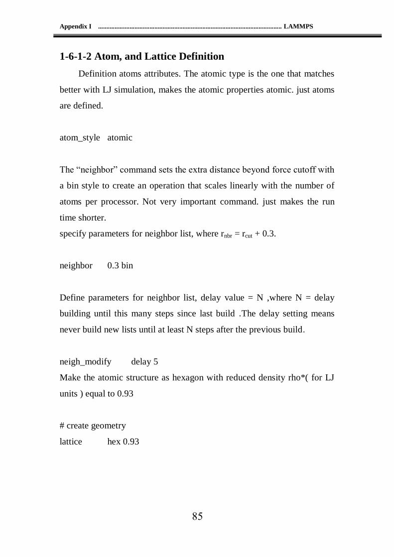
Appendix I ............................................................................................................... LAMMPS
77
1-6-1-2 Atom, and Lattice Definition
Definition atoms attributes. The atomic type is the one that matches
better with LJ simulation, makes the atomic properties atomic. just atoms
are defined.
atom_style atomic
The “neighbor” command sets the extra distance beyond force cutoff with
a bin style to create an operation that scales linearly with the number of
atoms per processor. Not very important command. just makes the run
time shorter.
specify parameters for neighbor list, where rnbr = rcut + 0.3.
neighbor 0.3 bin
Define parameters for neighbor list, delay value = N ,where N = delay
building until this many steps since last build .The delay setting means
never build new lists until at least N steps after the previous build.
neigh_modify delay 5
Make the atomic structure as hexagon with reduced density rho*( for LJ
units ) equal to 0.93
# create geometry
lattice hex 0.93
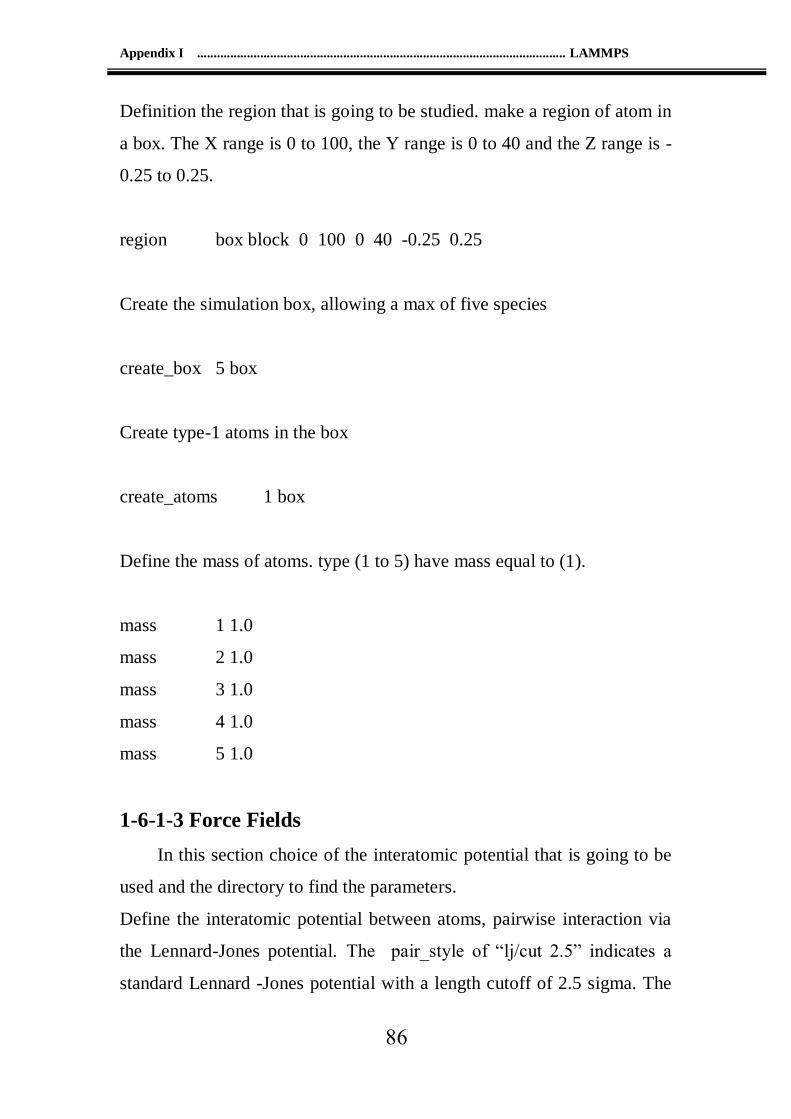
Appendix I ............................................................................................................... LAMMPS
77
Definition the region that is going to be studied. make a region of atom in
a box. The X range is 0 to 100, the Y range is 0 to 40 and the Z range is -
0.25 to 0.25.
region box block 0 100 0 40 -0.25 0.25
Create the simulation box, allowing a max of five species
create_box 5 box
Create type-1 atoms in the box
create_atoms 1 box
Define the mass of atoms. type (1 to 5) have mass equal to (1).
mass 1 1.0
mass 2 1.0
mass 3 1.0
mass 4 1.0
mass 5 1.0
1-6-1-3 Force Fields
In this section choice of the interatomic potential that is going to be
used and the directory to find the parameters.
Define the interatomic potential between atoms, pairwise interaction via
the Lennard-Jones potential. The pair_style of “lj/cut 2.5” indicates a
standard Lennard -Jones potential with a length cutoff of 2.5 sigma. The

Appendix I ............................................................................................................... LAMMPS
72
keyword “pair_coeff” sets the pairwise force field coefficients for one or
more pairs of atom types. An asterisk is used in conjunction with the( I,J)
types and means all types from 1 to N. Here, we set the coefficients to the
default value in epsilon and sigma.
# LJ potentials
pair_style lj/cut 2.5
The keyword “pair_coeff” sets the pairwise force field coefficients for
one or more pairs of atom types. An asterisk “*” is used in conjunction
with the I,J types and means all types from 1 to N. Here, set the
coefficients to the default value in epsilon and sigma. Where epsilon =
1.0, sigma = 1.0, cutoff = 2.5.
pair_coeff * * 1.0 1.0 2.5
1-6-1-4 Settings
Define groups of atoms, first should define region, then based on the
region define groups.
# define groups
In Group 1 in the X range is infinity to infinity, the Y range is infinity to
1.25 and the Z range is infinity to infinity.
region 1 block INF INF INF 1.25 INF INF
group lower region 1
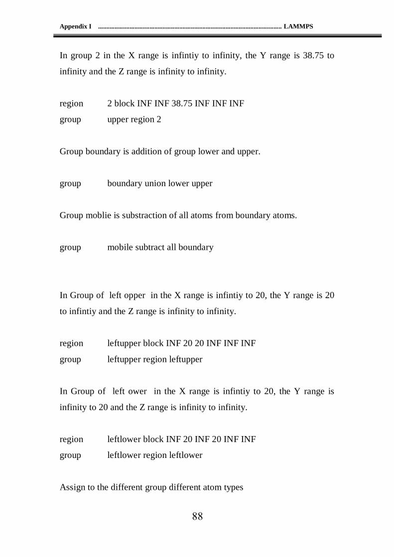
Appendix I ............................................................................................................... LAMMPS
77
In group 2 in the X range is infintiy to infinity, the Y range is 38.75 to
infinity and the Z range is infinity to infinity.
region 2 block INF INF 38.75 INF INF INF
group upper region 2
Group boundary is addition of group lower and upper.
group boundary union lower upper
Group moblie is substraction of all atoms from boundary atoms.
group mobile subtract all boundary
In Group of left opper in the X range is infintiy to 20, the Y range is 20
to infintiy and the Z range is infinity to infinity.
region leftupper block INF 20 20 INF INF INF
group leftupper region leftupper
In Group of left ower in the X range is infintiy to 20, the Y range is
infinity to 20 and the Z range is infinity to infinity.
region leftlower block INF 20 INF 20 INF INF
group leftlower region leftlower
Assign to the different group different atom types
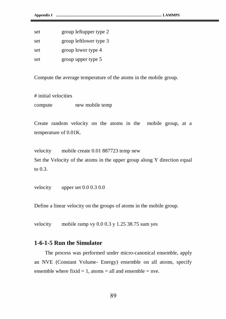
Appendix I ............................................................................................................... LAMMPS
77
set group leftupper type 2
set group leftlower type 3
set group lower type 4
set group upper type 5
Compute the average temperature of the atoms in the mobile group.
# initial velocities
compute new mobile temp
Create random velocity on the atoms in the mobile group, at a
temperature of 0.01K.
velocity mobile create 0.01 887723 temp new
Set the Velocity of the atoms in the upper group along Y direction equal
to 0.3.
velocity upper set 0.0 0.3 0.0
Define a linear velocity on the groups of atoms in the mobile group.
velocity mobile ramp vy 0.0 0.3 y 1.25 38.75 sum yes
1-6-1-5 Run the Simulator
The process was performed under micro-canonical ensemble, apply
an NVE (Constant Volume- Energy) ensemble on all atoms, specify
ensemble where fixid = 1, atoms = all and ensemble = nve.
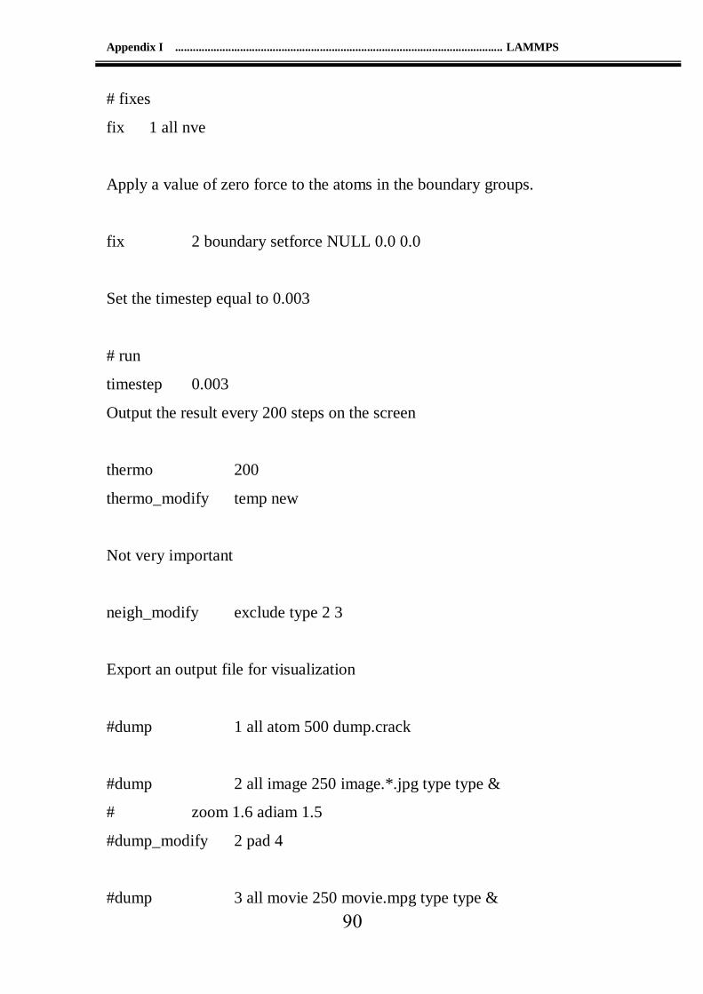
Appendix I ............................................................................................................... LAMMPS
78
# fixes
fix 1 all nve
Apply a value of zero force to the atoms in the boundary groups.
fix 2 boundary setforce NULL 0.0 0.0
Set the timestep equal to 0.003
# run
timestep 0.003
Output the result every 200 steps on the screen
thermo 200
thermo_modify temp new
Not very important
neigh_modify exclude type 2 3
Export an output file for visualization
#dump 1 all atom 500 dump.crack
#dump 2 all image 250 image.*.jpg type type &
# zoom 1.6 adiam 1.5
#dump_modify 2 pad 4
#dump 3 all movie 250 movie.mpg type type &
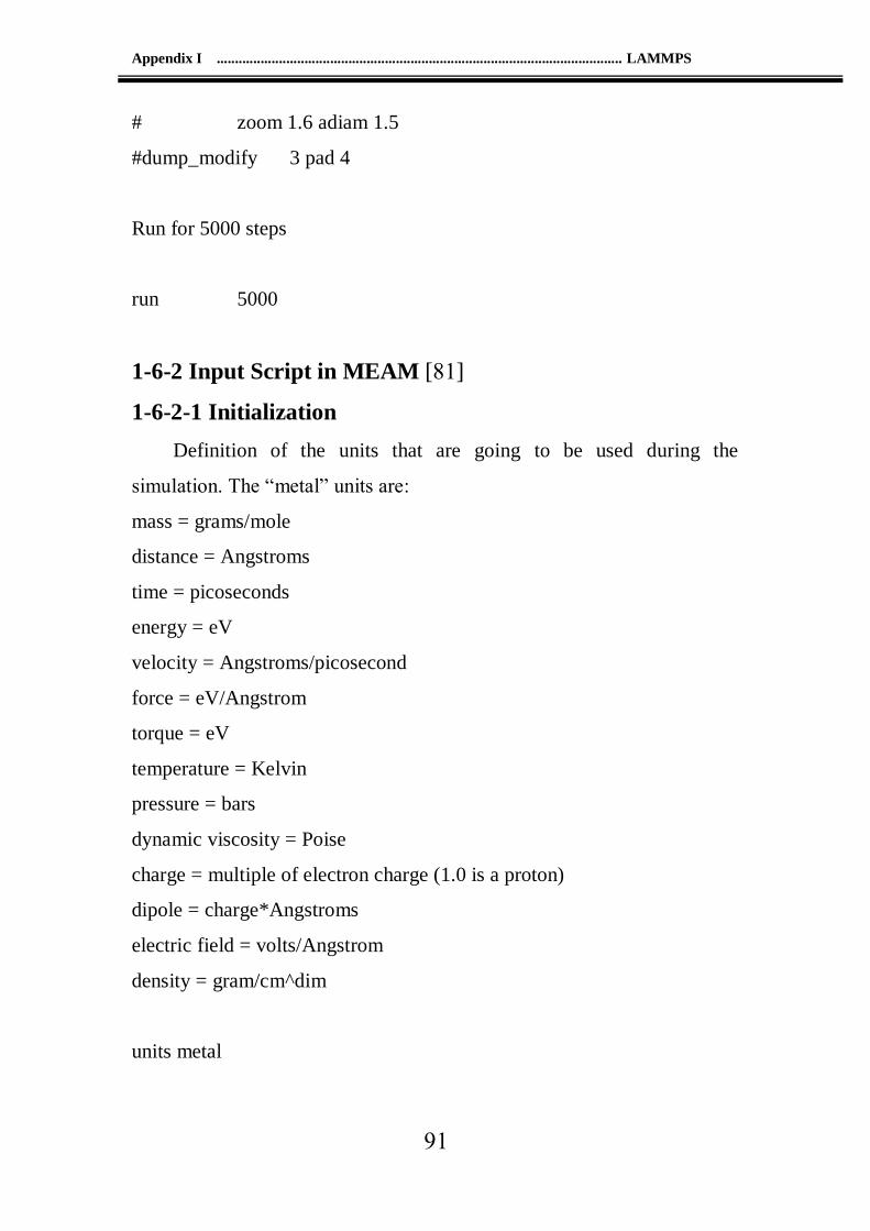
Appendix I ............................................................................................................... LAMMPS
78
# zoom 1.6 adiam 1.5
#dump_modify 3 pad 4
Run for 5000 steps
run 5000
1-6-2 Input Script in MEAM [78]
1-6-2-1 Initialization
Definition of the units that are going to be used during the
simulation. The “metal” units are:
mass = grams/mole
distance = Angstroms
time = picoseconds
energy = eV
velocity = Angstroms/picosecond
force = eV/Angstrom
torque = eV
temperature = Kelvin
pressure = bars
dynamic viscosity = Poise
charge = multiple of electron charge (1.0 is a proton)
dipole = charge*Angstroms
electric field = volts/Angstrom
density = gram/cm^dim
units metal

Appendix I ............................................................................................................... LAMMPS
77
Boundary conditions in each direction. For x, y and z directions the
boundary is periodic, which means that particles interact across the
boundary.
boundary p p p
1-6-2-2 Atom Definition
Definition atoms attributes. The atomic type is the one that matches
better with metal simulation, makes the atomic properties atomic.
just atoms are defined.
atom_style atomic
The “neighbor” command sets the extra distance beyond force cutoff with
a bin style to create an operation that scales linearly with the number of
atoms per processor. Not very important command. Just makes the run
time shorter.
specify parameters for neighbor list, where rnbr = rcut + 0.3.
neighbor 0.3 bin
define parameters for neighbor list, delay value = N ,where N = delay
building until this many steps since last build .The delay setting means
never build new lists until at least N steps after the previous build.
neigh_modify delay 10
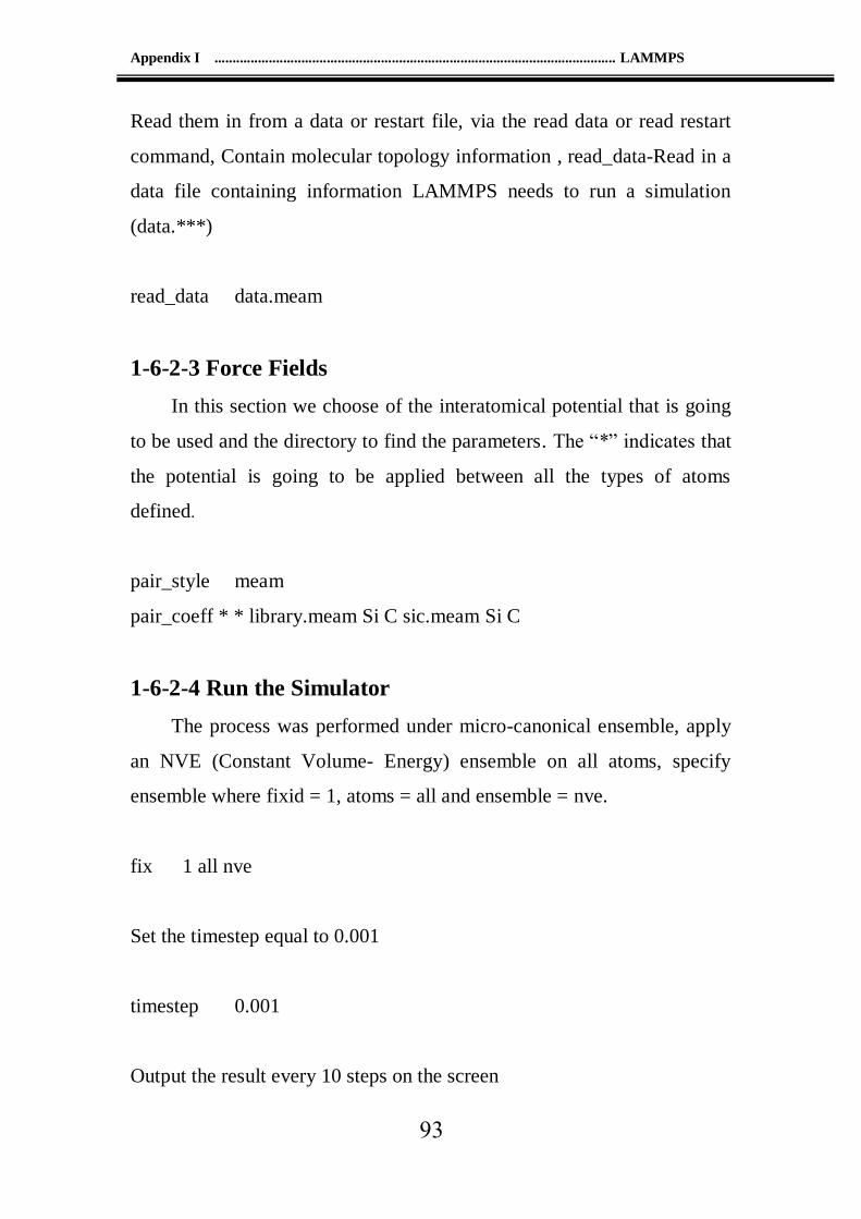
Appendix I ............................................................................................................... LAMMPS
77
Read them in from a data or restart file, via the read data or read restart
command, Contain molecular topology information , read_data-Read in a
data file containing information LAMMPS needs to run a simulation
(data.***)
read_data data.meam
1-6-2-3 Force Fields
In this section we choose of the interatomical potential that is going
to be used and the directory to find the parameters. The “*” indicates that
the potential is going to be applied between all the types of atoms
defined.
pair_style meam
pair_coeff * * library.meam Si C sic.meam Si C
1-6-2-4 Run the Simulator
The process was performed under micro-canonical ensemble, apply
an NVE (Constant Volume- Energy) ensemble on all atoms, specify
ensemble where fixid = 1, atoms = all and ensemble = nve.
fix 1 all nve
Set the timestep equal to 0.001
timestep 0.001
Output the result every 10 steps on the screen
Appendix I ............................................................................................................... LAMMPS
77
thermo 10
Export an output file for visualization
#dump 1 all atom 50 dump.meam
#dump 2 all image 10 image.*.jpg element element &
# axes yes 0.8 0.02 view 60 -30
#dump_modify 2 pad 3 element Si C
#dump 3 all movie 10 movie.mpg element element &
# axes yes 0.8 0.02 view 60 -30
#dump_modify 3 pad 3 element Si C
Run for 5000 steps
run 5000

REFERENCES
…………………….................................................................... References
84
1- Xinran Zhang ,” Computational Modeling of Li Diffusion Using
Molecular Dynamics”, A paper for graduation with Honors in Physics
faculty of the Department of Physics, Wake Forest University, (2015)
pp.1-31.
2- Satyanarayan Dhal and Yadlapalli Raja, “Effect of Size and Strain Rate
on Deformation Behaviour of Cu50Zr50 Metallic Glass: A molecular
Dynamics Simulation Study”, A Thesis of Department of Metallurgical
& Materials Engineering National Institute of Technology Rourkela-
769008, ( 2012) pp.1-63.
3- Ashis Das and Gaurav Singh, “ Plastic Deformation and failure studies
near a void for Copper-Aluminium alloy via Molecular Dynamics
Simulation”,
A thesis of Department of Metallurgical and Materials Engineering
National Institute of Technology, Rourkela, (2014) pp.1-50.
4- B.J. Alder and T. E. Wainwright, “ Studies in Molecular Dynamics. l”
,General Method, J. Chem. Phys. 31(2), (1959).
5- A. Rahman, “Correlations in the Motion of Atoms in Liquid Argon”,
Physics Review. 136 (2A), (1964) pp. 405-411.
6- Jarosaw Meller, “Molecular Dynamics”, Encyclopedia of Life Sciences,
Cornell University, Ithaca, New York, USA Nicholas Copernicus
University, Torun´, Poland, ( 2001) pp. 1-8.
7- Michael P. Allen, “Introduction to Molecular Dynamics Simulation”,
John von Neumann Institute for Computing, http://www.fz-juelich.de/nic-
series/volume23, (2004) pp. 1-28.
8- Xue Yang, “Atomistic Simulation Of Plasma Interaction With Plasma
Facing Components In Fusion Reactors”, PhD. Thesis, Purdue
University, West Lafayette, Indiana,(2013) pp. 1-141.
…………………….................................................................... References
85
9- William D. Callister, Jr.,“Fundamentals of Materials Science and
Enginerring” , John Wiley & Sons, Inc, University of Utah, (2001)
pp.147-196.
10- William G. Hoover, “Simulation of Brittle Fracture via Molecular
Dynamics”, G, lacucci (ed), Computer Simulation in Physical
Metallurgy- © ECSC, EEC, EAEC, Brussels and Luxemhourg, (1986)
pp. 145-158.
11- Mnrray S., Daw and Michael I. Baskes, “Application of the embedded
atom method to hydrogen embrittlement”, Springer Science, (1987) pp.
196-213.
12- Mnrray S. Daw and M. I. Baskes “Embedded-atom method: Derivation
and application to impurities, surfaces, and other defects in metals”,
Physical Review B, V.29, N.12, ( 1984) pp. 6443-6453.
13- Mnrray S. Daw and M. I. Baskes, “Semiempirical, quantum mechanical
calculation of hydrogen embrittlement in metals”, Physical Review
Letters , V.50, N.17, ( 1983) pp. 1285–1288.
14- Mnrray S. Daw , Stephen M. Foiles and Michael I. Baskes “The
embedded-atom method: A review of theory and applications”, Materials
Science Reports- Elsevier Science Publishers B.V. All rights reserved, (
1993) pp. 251–310.
15- S. Nouranian, M.A. Tschopp, S.R. Gwaltney, M.I. Baskes, and M.F.
Horstemeyer, “An interatomic potential for saturated hydrocarbons based
on the modified embedded-atom method”, physics.chem-ph., (2014) pp.
1–29.
16- CH. Henager, Jr., F. Gao, SY. Hu, G. Lin, EJ. Bylaska and N. Zabaras,
“Simulating Interface Growth and Defect Generation in CZT –Simulation
State of the Art and Known Gaps. Pacific Northwest National

…………………….................................................................... References
86
Laboratory”, Report- Prepared for the U.S. Department of Energy under
Contract DE-AC05-76RL01830,USA, (2012) pp. 1-81.
17- M.I. Baskes, “The Modified Embedded Atom Method. Association for
information and image management” ,Assoclation for information and
image Management 1100 wayne Avenue, Suite 1100 Silver Spring,
Maryland 20910 (1994) pp. 3-28.
18- Daan Frenkel and Berend Smit, “Understanding Molecular Simulation for
Algrithms to Application” .University of Amsterdam the Netherlands,
Academic Press A Division of Harcourt, Inc. (2002) pp. 1-658.
19- Michele Meo and Marco Rossi, “Prediction of Young’s modulus of single
wall carbon nanotubes by molecular-mechanics based finite element
modeling”, Composites Science and Technology, Department of
Mechanical Engineering, University of Bath, Claverton Down, Bath BA2
7AY, (2006) pp. 1597–1605 .
20- Erik Fransson and Johannes Laurell Hakansson “Local and Global
Ordering in Barium Zirconate, a Model Potential Study”, Thesis for the
degree of Master of Science in Engineering Physics, Department of
Applied Physics Division of Materials and Surface Theory Chalmers
University of Technology Gothenburg, Sweden, (2014) PP.1-58.
21- Lammps molecular dynamics simulator, http://lammps.sandia.gov/
,(2014).
22- Wang, Mingchao, Yan, Ceng, Ma, Lin, Hu, Ning and Chen, Mingwei,
“Effect of defects on fracture strength of graphene sheets”
,Computational Materials Science,(2012) pp. 236-239.
23- Bohumir Jelinek, Sabastien Groh, Mark F. Horstemeyer, Jeffery Houze,
Seong-Gon Kim, Gregory J. Wagner,Amitava Moitra and Michael I.
Baskes, “Modified embedded atom method potential for Al, Si, Mg, Cu,
…………………….................................................................... References
87
and Fe alloys”, Physical review.B, Condensed matter
85(24):245102,(2012).
24- Minh-Quy Le and Romesh C. Batra , “Single-edge crack growth in
graphene sheets under tension” , Computational Materials Science,
(2013) pp. 381-388.
25- G. D. Samolyuk, Stas I. Golubov, Y. N. Osetsky, and R. E. Stoller,
“Molecular dynamics study of influence of vacancy types defects on
thermal conductivity of β-SiC”, Journal of Nuclear Materials 418, (2011)
pp. 174-181.
26- Mazdak Ghajari, Lorenzo Iannucci and P. T. Curtis, “A peridynamic
material model for the analysis of dynamic crack propagation in
orthotropic media”, Computer Methods in Applied Mechanics and
Engineering 276, (2014) pp. 431-452.
27- Laalitha S. I. Liyanage, Jeff Houze, Sungho Kim, Mark A. Tschopp,
Seong-Gon Kin, Michael I. Baskes and Marks F. Horstemeyer,
“Structural, elastic and thermal properties of cementite(Fe3C) calculated
using Modified Embedded Atom Method”, Physical Review B 89,
(2014).
28- Alireza Tabarraei and Xiaonan Wang, “A molecular dynamics study of
nanofracture in monolayer boron nitride”, Materials Science &
Engineering A 641, (2015) pp. 225-230.
29- Ebrahim Asadi , Mohsen Asle Zaeem, Sasan Nouranian, and Michael I.
Baskes, “Two-phase solid–liquid coexistence of Ni, Cu, and Al by
molecular dynamics simulations using the modified embedded-atom
method”, Science Direct, Acta Materialia 86, (2015) pp. 169-181.
30- Qi-lin Xiong, Zhen-huan Li and Xiao-geng Tian, “Fracture behaviors of
pre-cracked monolayer molybdenum disulfide: A molecular dynamics
study” , Beilstein Journal of Nanotechology, (2016) pp. 1411-1420.

…………………….................................................................... References
88
31- Naigen Zhou, Chi Zhang, Xiang Zeng, Jiren Yuan and Lang Zhou, “A
molecular dynamics study of the growth rate of SiC crystal and its
dependence on the temperature” , Interational Journal of Modern Physics
B, Volume 30 (2016) pp. 1-12.
32- Lu Xie, “Simulations du dépôt par pulverization plasma et de la
croissance de couches minces”, PhD. thesis, UniversIté D’orléans, (2013)
PP.1-155.
33- Dhatri Gaddamanugu,“Finite Element Modelling and Molecular Dynamic
Simulations of Carbon Nanotubes/Polymer Composites”. Texas A&M
University, (2009) pp.1-83.
34- Hoang,K.C.; Fu,Y. and Song,J.H. “An hp-proper orthogonal
decomposition–moving least squares approach for molecular dynamics
simulation”. Computer Methods Applied Mechanics Engineering,
University of Colorado at Boulder, Boulder, CO 80309, (2016) pp.548–
575.
35- Fredrik Hedman, “Algorithms for Molecular Dynamics Simulations”.
Stockholms University, (2006) pp.1-93.
36- J. M. Seminario and Perla B. Balbuena, “Molecular dynamics: From
classical to Quantum methods” . Theroretical and computational
chemistry, University Columbia U.S.A., (1999) pp.1-946.
37- Maria Cano Colino, “Molecular Dynamics Simulation of EPSP
Synthase”. Universitat Autònoma de Barcelona, (2007) pp.1-41.
38- A.J. Stone, “The theary of intermolecular forces”, Clarendon
Press.Oxford, Department of Chemistry ,University Cambridge, (1996)
pp. 1-41.
39- Gemma Safont Camprubí ,“Mechanical properties at nano-level”,
University Lund, (2011) pp.1-28.

…………………….................................................................... References
011
40- Nneoma Ogbonna ,“Molecular Dynamics Simulation” . African Institute
for Mathematical Sciences Muizenberg, South Africa., (2004) pp. 2-37.
41- Mihai Ciocoiu,“Materials behavior : Research methodology and
mathematical models”, CRC Press, Taylor& Francis Group, Apple
Academic Press, (2015) pp.1-361.
42- Sale,K.L. “Molecular Modelig of Nitroxidesspin Labels: Methods
Development and Applications”. The University Florida ,College of Arts
and Sciences, (2002) pp.1-325.
43- Rangel-Vazquez,N.A. and felix, F.R. “Computational Chemistry Applied
in the Analyses of Chitosan /Polyvinylpyrrolidone/ Mimosa Tenuiflora” .
Science Publishing Group, (2014) pp.1-97.
44- Robert K. Poole, “Globin and other Nitric oxide -Reactive proteins, part
B”, Department of Molecular Biology and Biotechnology , The
University of Sheffield, UK, (2008) pp.1-654..
45- H. Fehske, R. Schneider, and A. Weibe, “Computational many-particle
physics”,Springer, (2008) pp.1-780.
46- Jiaxi Zhang, “Molecular dynamics study of crack propagation behavior
and mechanisms in Nickel”, MSC. Thesis, The Ohio State University,
(2011) pp.1-58.
47- Beena Rai,“Molecular modeling for the design of novel performance
chemical and materials”, CRC Press, Taylor& Francis Group, pp.1-382.
(2012).
48- Daniel Schopf, “Effective Potentials for Numerical Investigations of
Complex Intermetallic Phases”, Institut für Theoretische and Angewandte
Physik ,Universität Stuttgart, (2013) pp.17-238.
49- Kivilcim Basak Vural,” Adsorption of Gold Atoms on Anatase
TiO2(100) -1×1 Surface”, MSc. Thesis, University Middle East
Technical , (2009) pp.1-50.
…………………….................................................................... References
010
50- John A. Keith, Josef Anton, Payam Kaghazchi, and Timo Jacob,
“Modeling Catalytic Reactions on Surfaces with Density Functional
Theory. 1st ed”, (2012) pp.1-38.
51- Stefan Wippermann, “Understanding substrate-supported atomic-scale
nanowires from ab initio theory”, University Paderborn, (2010) pp.1-184.
52- Kim, lurii, “First-principles study on electronic and structural properties
of Cu(In/Ga)Se alloys for solar cells”, University Lappeenranta of
Technology, LUT school of Technology, Department of Mathematics and
Physics, (2015) pp.1-40.
53- Vorgelegt Von, “Interface Dipole Formation in Organic Surface
Functionalizations”, PhD. Thesis, Von der Fakultät für Mathematik,
Informatik und Naturwissenschaften der RWTH Aachen University,
(2012) pp. 8-274.
54- Fabiano Corsetti, “On the properties of point defects in silicon
nanostructures from ab initio calculations”, PhD. Thesis ,Thomas Young
Centre ,Imperial College London, (2012) pp.1-259.
55- S. Dalgic, and S. Guler, “The Atomic Structure of Lattice Mismatched
Si/Ge Bulk Heterostructures by Using the Density Functional Theory”,
Physics Department, Faculty of Science, Trakya University, 22100,
Edirne (TURKEY) (2011) pp.1-4.
56- Geoffrey Tse, “Study of Piezoelectricity on III/V semiconductors from
atomistic simulations to computer modeling”, PhD. Thesis , University of
Manchester, (2012) pp.1-213.
57- Samir Lounis,“Theory of Magnetic Transition Metal Nanoclusters on
Surfaces”, Reihe Materie und Material / Matter and Materials,41(2007)
pp.1-189.
58- EVA D. Zurek,”Density Functional Theory (DFT) Studies of Solids and
Molecules”, PhD. Thesis ,University Stuttgart, (2006) pp.7-161.

…………………….................................................................... References
011
59- Sara Galasso, “Generalization of the Eliashberg equations and Density
Functional Theory applied to the analysis of the fundamental properties
of iron-basedsuperconductors”, PhD. Thesis, Politecnico di Torino, Porto
Institutional Repository, (2015) pp.1-84.
60- Jiawei Xian, “Electronic Properties of Gold Nanoclusters from GW
Calculations”, PhD. Thesis, pp.1-109 (2012).
61- Sami Auvinen, “Computational Modeling of The Properties of TiO2
Nanoparticles”. University Lappeenranta of Technology,(2013) pp.13-59.
62- Vorgelegt Von, “Surface Functionalization with Amino-based Self-
Assembled Monolayers”, PhD. Thesis, Von der Fakultät für Mathematik,
Informatik und Naturwissenschaften der RWTH Aachen University,
(2015), pp.1-211.
63- Mohammed Suleiman Hussein Suleiman,”Theoretical Investigation of
Structural, Electronic and Optical Properties of some Group10,11 and
12Transition-Metal Nitrides”, PhD. Thesis ,University Witwatersrand,
Johannesburg, (2013) pp.1-278.
64- Paolo Giannozzi, Scuola Normale Superiore and Piazza dei Cavalieri,
“Density Functional Theory For Electronis Structure Calculations”,
Università di Pisa, (2005) pp.1-35.
65- Jianlin Chang, “Ab initio calculations of semiconductor surfaces and
molecular clusters”, PhD. Thesis, Queen's University Kingston, Ontario,
Canada , (1997) pp.1-139.
66- MARAL Mianpour, “Theoretical Studies of Nanostructure Formation and
Transport on Surfaces”, PhD. Thesis ,University of Central Florida,
(2013) pp.1-208.
67- R.M. Martin, “Pseudopotentials”, Cambridge University, (2004) pp.205-
231.
…………………….................................................................... References
012
68- Jian-Hua Zhang, Shun-Qing Wu, Yu-Hua Wen, and Zi-Zhong Zhu, “An
EAM potential for the dynamical simulation of Ni-Al alloys Journal
Atomic Molecular Sciences”, Department of Physics and Institute of
Theoretical Physics and Astrophysics, Xiamen University, Fujian
361005, China, Vol. 1, No. 3,(2010) pp. 253-261.
69- S.Y. Hu, M.I. Baskes, M. Stan, and L.Q. Chen, “Atomistic calculations of
interfacial energies, nucleus shape and size of h0 precipitates in Al–Cu
alloys”. Acta Materialia, 54, (2006) pp. 4699–4707.
70- M.I. Baskes, “Modified embedded-atom potentials for cubic materials
and impurities”, physical Review B, Vol. 46, NO. 5, (1992) pp. 2727-
2742.
71- Hanchen Huang, Nasr M. Ghoniem, J immy K. Wong, and Michael I.
Baskest, “Molecular dynamics determination of defect energetics in B-
Sic using three representative empirical potentials”, Modelling and
Simulation in Materials Science and Engineering, University of
California, (1995) pp.615-627.
72- Markus J. Buehler and Huajian Gao, “Chapter 1 modeling dynamic
fracture using large-scale atomistic simulations”, Massachusetts Institute
of Technology, Department of Civil and Environmental Engineering 77
Massachusetts Avenue Room 1-272, Cambridge, MA., 02139, USA,
(2007) pp. 1-67.
73- Kristian Berg Keilen, “Polymer failure modeled by Molecular
Dynamics”, Materials Science and Engineering, Norwegian University
of Science and Technology, Department of Engineering Design and
Materials, (2014) pp. 1-127.
74- Farid, F. Abraham, Dominique Brodbeck, William E. Rudge and
Xiaopeng Xu, “A molecular dynamics investigation of rapid fracture
mechanics”. IBM Research Division, Almaden Research Center, 650

…………………….................................................................... References
013
Harry Road, San Jose, CA 95120-6099, U.S.A. ,Vol. 45, No. 9, (1997)
pp. 1595-1619.
75- Petucci,J.; LeBlond,C and Karimi M. Molecular dynamics simulations of
brittle fracture in fcc crystalline materials in the presence of defects. pp.
130-139. (2014).
76- Ravi Kiran Siripurapu, “Molecular Dynamics Study of Zirconium and
Zirconium Hydride”, MSc. Thesis, Department of Mechanical
Engineering, University of Saskatchewan, (2013) pp. 1-94.
77- Tommy Andersson, “One-shot free energy calculations for crystalline
materials”, MSc. Thesis, University chalmers of technology, (2012) pp.
1-57.
78- Justin M. Petucci, “A Study of crack propagation in metals in the
presence of defects”, MSc. Thesis, Indiana University of Pennsylvania,
(2013) pp. 1-104.
79- http://katter-world.blogspot.com/2010/05/install LAMMPS on ubuntu.
80- David Keffer, “Evaluating Thermodynamic properties in LAMMPS”,
Department of Materials Science & Engineering University of Tennessee,
Knoxville, (2016) pp. 1-10.
81- LAMMPS User’s Manual .http://lammps.sandia.gov. (2016).
82- Nneoma Ogbonna, “Molecular dynamics simulation”, African Institute
for Mathematical Sciences, (2004).
الخلاصت
( ببسخخذام MEAMوحؼذيل طشيقت غوش الزسة ) الخصذع , حن دساستالشسبلتفي ز
شبيكت السذاسيت وفي حؼذيل الفي خصذعلشش ال( lammpsهحبكبة ), الوحبكبة الذيبهيكيت الجضيئيت
خلاػبثالا شوء حخضوي الخصذع هيكبيكيت . (SiC) السليكوى كبسبيذ وبدةطشيقت غوش الزسة ل
.غيش الوخكبهل الخشاص حوليذو
, 0..., 0..., 0...,..........) كبج الخطواث الضهيت الوسخخذهتالخصذع كودفي
و 0...., 0...., 0...., ....., 0...., 0...., 0...., 0...., 0....
(reduced 0.00001 0....) الوسخخذهت خطواث الضهيتالوفي حؼذيل طشيقت غوش الزسة ,
, ( 0Ps.....و 0....., 0....., 0....., 0....., 0....., 0...., 0....
صغيشة بوب يكفي لضوبى الحفبظ ػلي الطبقت وحجب الاخطبءيجب اخخيبسب الخطوة صهيت
ي الخصذع كود فيهخخبسة خطوة صهيت وببلخبلي فبى افضل , الوفصلت كبيشةال
(......0reduced ) 0.....) يوفي حؼذيل طشيقت غوش الزسة(Ps . الخصذعفي كود
يبذا حيي و ػذم ابخذاء الخصذع,بسبب ()القصبى في السبلبي لطبقت الكبهتفي اضيبدة ال
خطوة الخشغيل في 302511ϵ-فبى قيوت الطبقت الكبهت حكوى هسبويت الي ببلخوسغ الخصذع
بيوب الضيبدة في دسجت الحشاسة حشيش الي حكسش الاواصش بيي الزساث, وز بحج هي, ..0.0
في الضغظ للظبم بسبب ػذم شوء الخصذع )القصبى في السبلبي( الضيبدةاخشبس الخصذع .
في الضغظ بسبب حكسش الاواصش بيي الزساث ػذ اخشبس السبلبي( )الضيبدة في قصبىوهي ثن ال
و ثببج.صذع خلاحجن او هسبحت في زا الكود فبى . الخصذع
لاى غوش تسبلببلب الطبقت الكبهتفي ضيبدة ال( , MEAMفي حؼذيل طشيقت غوش الزسة )
هي اجل كسش الاواصش بيي كبفيت رسة بوجووػت هي الزساث )ظبم هسخقش( ححخبج الي طبقت
للظبم يوكي اى حؼضى الي الضيبدة السشيؼت والوضطشدة في حكسش الطبقت الحشكيتصيبدة الزساث. و
الظبم دسجت حشاسة الظبم هحفوظت فبى . ػلي الشغن هي طبقت الاواصش بيي الزساث الووضؼيت
و بيي الزساث. واصشكسش الاحالطبقت الكبهت الي طبقت حشكيت خيجت ححويل حضداد ػذهب يخن
خيجت كسش الاواصش بيي الزساث الضغظ ببلسبلبيضداد

جوهىريت العراق
وزارة التعلين العالي والبحث العلوي
كليت التربيت/جاهعت القادسيت
الفيسياءقسن
محاكاة الباستخدام SiCمادة لخصائص الميكانيكية الدراسة
(LAMMPSالجزيئية ) الديناميكية
جامعة القادصية /مجلش كلية الحربية إلىرصالة مقدمة
الفيزياء علىم في وهي جزء من محطلبات نيل درجة الماجضحير
جقدمث بها
حيدر عبد النبي الوحنت شروق
كلية الحربية /فيزياء سبكالىريى
2014 جامعة القادصية
بأشراف
البيرهاني حسن هشام هحود عليد .م.أ
م 2017 هـ1438


![Mechanical and tribological properties of AA7075–TiC metal ... · Unlu et al. [14] proved that the mechanical properties of aluminum matrix composites reinforced by Al2O3 and SiC](https://img.pdfslide.us/doc/110x75/6031f73f4f7e7c75a330c69c/mechanical-and-tribological-properties-of-aa7075atic-metal-unlu-et-al-14.jpg)