Embed Size (px)
Citation preview
862d Session* J JOINT COMMITTEE PRINT
STUDY PAPER NO. 21
P O STW A R M O V E M E N T OF PRICES A N D
W A G E S IN M A N U F A C T U R IN G
IN D U ST R IE SBY
H arold M . L evin so n
AND
SUPPLEMENTARY TECHNICAL MATERIAL TO THE STAFF REPORT
BY
G e o r g e W . B l e i l e a n d T h o m a s A . W i l s o n
MATERIALS PREPARED IN CONNECTION WITH THE
STUDY OF EMPLOYMENT, GROWTH, AND PRICE LEVELS
FOR CONSIDERATION BY THE
JOINT ECONOMIC COMMITTEE CONGRESS OF THE UNITED STATES
JANUARY 30, 1960
Printed for the use of the Joint Economic Committee
UNITED STATES
GOVERNMENT PRINTING OFFICE 60505 WASHINGTON : 1960
For sale by the Superintendent of Documents, U.S. Government Printing Office Washington 25, D.O. - Price 40 cents
Digitized for FRASER http://fraser.stlouisfed.org/ Federal Reserve Bank of St. Louis
JOINT EC O N O M IC C O M M IT T E E(Created pursuant to sec. 5(a) of Public Law 304, 79th Cong.)
PAUL H. DOUGLAS, Illinois, Chairman WRIGHT PATMAN, Texas, Vice Chairman
SENATE
JOHN SPARKMAN, Alabama J. WILLIAM FULBRIGHT, Arkansas JOSEPH C. O’MAHONEY, Wyoming JOHN F. KENNEDY, Massachusetts PRESCOTT BUSH, Connecticut JOHN MARSHALL BUTLER, Maryland JACOB K. JAVITS, New York
HOUSE OF REPRESENTATIVESRICHARD BOLLING, Missouri HALE BOGGS, Louisiana HENRY S. REUSS, Wisconsin FRANK M. COFFIN, Maine THOMAS B. CURTIS, Missouri CLARENCE E. KILBURN, New York WILLIAM B. WIDNALL, New Jersey
Stu d y of E m p lo ym e n t , G r o w t h , a n d P rice L ev e ls
(Pursuant to S. Con. Res. 13, 86th Cong., 1st sess.)O t t o E c k s t e i n , Technical Director
J o h n W. L e h m a n , Administrative Officer J a m e s W. K n o w l e s , Special Economic Counsel
n
Digitized for FRASER http://fraser.stlouisfed.org/ Federal Reserve Bank of St. Louis
This is part of a series of papers being prepared for consideration by the Joint Economic Committee in connection with its “Study of Employment, Growth, and Price Levels.” The committee and the committee staff neither approve nor disapprove of the findings of the individual authors.
m
Digitized for FRASER http://fraser.stlouisfed.org/ Federal Reserve Bank of St. Louis

Digitized for FRASER http://fraser.stlouisfed.org/ Federal Reserve Bank of St. Louis
LETTERS OF TRANSMITTAL
To Members of the Joint Economic Committee:Submitted herewith for the consideration of the members of the
Joint Economic, Committee and others is study paper No. 21, “Postwar Movement of Prices and Wages in Manufacturing Industries.”
This is among the number of subjects which the Joint Economic Committee requested individual scholars to examine and report on in connection with the committee’s study of “Employment, Growth, and Price Levels.”
The findings are entirely those of the authors, and the committee and the committee staff indicate neither approval nor disapproval by this publication.
P a u l H . D o u g l as , Chairman, Joint Economic Committee.
Ja n u a r y 18 , 1 9 6 0 .
Ja n u a r y 12, 1960.Hon. P a u l H. D ouglas ,Chairman, Joint Economic Committee,U.S. Senate, Washington, D .C .
D e a r S e n a t o r D o u g l a s : Transmitted herewith is one of the series of papers prepared for the study of “Employment, Growth, and Price Levels” by outside consultants and members of the staff. The author of this paper is Harold M. Levinson of the University of Michigan.
All papers are presented as prepared by the authors.O tto E c k st e in ,
Technical Director,Study of Employment, Growth, and Price Levels.
Digitized for FRASER http://fraser.stlouisfed.org/ Federal Reserve Bank of St. Louis

Digitized for FRASER http://fraser.stlouisfed.org/ Federal Reserve Bank of St. Louis
C O N T E N T S
I. Introduction___________________________________________________ 1Sources and limitations______________________________________ 1
II. Wage movements in the postwar period__________________________ 2Wage patterns in the postwar period-------------------------------------- 7
III. The movement of manufacturing prices___________________________ 13Trends in specific manufacturing industries----------------------------- 17Sources and limitations of data______________________________ 19
IV. Summary______________________________________________________ 21
APPENDIXESAppendix A. Sources of basic data________________________________________23Appendix B. Cross-section correlation matrixes________________________ ____49Appendix C. Trends in individual industries relative to all manufacturing. 54
TABLESTable 1. Simple cross-section correlation coefficients between wage changes
and selected variables, 1947-58-------------------------------------------------------- 3Table 2. Cross-section regress equations: Wages----------------------------------- 4Table 3. Simple time series correlation coefficients between annual changes
in wages and selected variables, 1947-58____________________________ 5Table 4. Time series partial correlation coefficients between annual changes
in wages and employment and profits, 1947-58---------------------------------- 6Table 5. Changes in wages, profit rates, concentration ratios, union
strength, and employment in manufacturing industries, 1947-53 and1953-58__________________________________________________________ 7
Table 6. Wage-fringe adjustments in selected manufacturing industries,1946-58__________________________________________________________ 8
Table 7. Basic trends in the steel and automobile industries, 1947-58__ 11Table 8. Wholesale price indexes in manufacturing industries, 1947-58 __ 14 Table 9. Simple cross-section correlation coefficients between price
changes and selected variables, 1947-58-------------------------------------------- 15Table 10. Cross-section regression equations: Prices___________________ 16Table 11. Simple time series correlation coefficients between annual
changes in prices and selected variables, 1947-58____________________ 17Table 12. Time series partial correlation coefficients between annual
changes in prices, output, and hourly earnings, 1947-58---------------------- 17Table 13. Basic trends in all manufacturing, 1947-58__________________ 18Table 14. Ratio of indexes in specific industries relative to all manufactur
ing, 1947-58______________ __________ _____________________________ 20SUPPLEMENTAL STAFF MATERIAL TO THE STAFF REPORT
Technical Note No. 1— The service section: Data on output, employment,prices, and income, by George W. Bleile_____________________________ 63
Technical Note No. 2—Productivity and output in the postwar period, by Thomas A. Wilson_______ ___________ _____________________________ 129
vn
Page
Digitized for FRASER http://fraser.stlouisfed.org/ Federal Reserve Bank of St. Louis
STUDY PAPER NO. 21
POSTW AR M O VEM E N T OF PRICES AND W AGES IN MANUFACTURING INDUSTRIES
I . I n t r o d u c t io n 1
This study paper is designed primarily to present the underlying data and the statistical procedures developed as part of the analysis of the postwar inflation prepared for consideration by the Joint Economic Committee of the Congress.2 In general, the present report does not attempt to carry the analysis of the data beyond that already presented in the staff report; rather, the major purpose is to make the basic data generally available, and to present the results of the various statistical procedures which were employed in analyzing the movement of wages, prices, and profits in manufacturing industries from 1947 to 1958.
S o u r c e s a n d L im it a t io n s
In order to evaluate the major factors which might underlie these movements in the several manufacturing sectors of the economy during the period since 1947, data for a number of variables were obtained for each of 19 2-digit Standard Industrial Classifications in manufacturing. All of these basic series are presented in appendix A, together with a description of the sources and methodology used. At this point, however, a number of technical aspects of the data should be noted.
Of particular importance is the fact that the underlying figures were gathered by different Government agencies, often utilizing different sampling techniques and different methods of classification. Thus the data on earnings and employment were obtained on an establishment basis, with each establishment assigned to a particular industry on the basis of its principal product, measured in value terms. The figures for profits, sales, stockholders’ equity, and depreciation and depletion, on the other hand, were obtained by the FTC-SEC on a corporation wide basis; the data for the entire corporation were then assigned to the industrial classification on the basis of the corporation’s
11 have received much helpful assistance from several Government agencies in the course of preparing the present study. In particular, I would like to express my appreciation to Harry Douty and Lily Mary David of the BLS Division of Wages and Industrial Relations; to Sidney Jaffe, Allan Searle, and Helen Hald of the BLS Division of Prices and Cost of Living; to Jack Alterman of the BLS Division of Productivity; to Gladys Miller, Robert Stein, and Sophia Cooper of the BLS Division of Manpower and Employment; to Hyman Lewis of the BLS Office of Labor Economics; and to Louis Paradiso of the U.S. Department of Commerce. Thomas Wilson of the staff of the Joint Economic Committee provided es- tensive help in the statistical computations; and Stanley Heckman and Hamilton Gewehr provided general assistance throughout.
2 For the general discussion of the postwar inflation, see the “Staff Report on Employment, Growth, and Price Levels,” ch. V. (Government Printing Office, Dec. 24, 1959).
1
Digitized for FRASER http://fraser.stlouisfed.org/ Federal Reserve Bank of St. Louis
principal product, measured in terms of annual sales volume. And finally, concentration ratios were computed from data based on the value of product shipments directly, irrespective of the establishment or corporation involved.
As a result of these differences in concept and scope, the several series are not completely comparable. To a substantial degree, however, the varying bases of classification are probably corrected by the fact that the 2-digit industry classifications used here are quite broad; consequently, they would normally embrace both the primary and the great majority of secondary products produced by any given establishment. In the case of corporatewide classification, however, there is a greater possibility that the profits figures will be overstated or understated. Classification on a product basis directly, of course, raises no serious issues.
The meaning and limitations on the use of concentration ratios also deserve some preliminary discussion. In general, concentration ratios provide a measure of tne proportion of the total value of shipments or of total employment in a particular manufacturing industry which is accounted for by the largest companies in that industry. As such, they may provide a rough measure of the extent of competitive pressures existing in the product market, on the presumption that the larger the proportion of the product value which is sold by the largest firms, the greater is the “degree of monopoly” involved. There are, however, important limitations on the use 01 concentration ratios for this purpose. On the one hand, such ratios do not reflect the pressure of competition from substitute products, such as plastics for metals; nor do they reflect the extent to which imports may compete in the domestic market. As a result, concentration ratios may overstate the degree of monopoly in a particular situation. On the other hand, these ratios do not reflect the extent to which the relevant product market may be regional or local in character, as in the case of goods having high transportation costs. In these instances, ratios based on product value shipments for the entire country tend to understate the effective degree of concentration.3 Nevertheless, concentration ratios can provide at least a general frame of reference for evaluating whether a particular industrial classification is “more” or “less” competitive.
II. W a g e M o v e m e n t s in t h e P o s t w a r P e r i o d
A number of statistical analyses were carried out relating the percentage changes in straight time hourly earnings in the 19 manufacturing industries with the movements of several other variables, including the percentage changes in production worker employment, output, productivity per production worker man-hour, the level of profits (as a rate of return on equity), and concentration ratios.
Some of thQ, results of a complete year-to-year cross section analysis are summarized in table 1; in addition, a complete matrix of all possible simple correlation coefficients is shown in appendix B.4 The simple coefficients listed in table 1 suggest several important points’ Of considerable interest is the fact that no significant relationship was
3 An excellent presentation of these and other limitations on the use of concentration ratios can be found in “Concentration in American Industry,” Subcommittee on Antitrust and Monopoly, at pp. 3-6.
4 All the regressions and correlation coefficients presented in the following discussion are single equation least squares estimates. All equations fitted were linear.
2 PRICES AND WAGES IN MANUFACTURING INDUSTRIES
Digitized for FRASER http://fraser.stlouisfed.org/ Federal Reserve Bank of St. Louis
evident between the year-to-year changes in earnings and percentage changes in output, production worker employment, or productivity per production worker man-hour. On the other hand, the data indicate a strong interrelationship, particularly after 1951, between hourly earnings, profit levels, and 1954 concentration ratios. With the exception of the year 1955-56, earnings and profits were very highly correlated; the relationship of earnings to concentration ratios, while weaker, was still quite marked.
PRICES AND WAGES IN MANUFACTURING INDUSTRIES 3
T a b l e 1.— Simple cross section correlation coefficients between wage changes and selected variables in 19 manufacturing industries} 1947-581
Year
Straight time earnings on—
Outputon
profitsbeforetaxes
Concentration ratios on—
Production
workeremploy
ment
Productivity
per production worker man- hour
OutputProfitsbeforetaxes
Profitsaftertaxes
Concentra
tionratios
Profitsbeforetaxes
Profitsaftertaxes
1947-48................................... 0.417 -0.248 0.195 0.012 0.138 0.226 0.463 -0.108 0.0711948-49................................... —.050 .162 .024 .616 .777 .336 .237 .447 .5271949-50................................... -.563 .362 -.372 -.087 -.097 .033 .654 .307 .3401950-51................................... .171 -.247 .078 .178 .127 .045 .631 .361 .3711951-52................................... .087 .118 .039 .598 .707 .283 .491 .458 .4631952-53................................... .249 .251 .332 .550 .689 .423 .724 .569 .5371953-54................................... .203 -.279 -.067 .628 .520 .463 -.059 .553 .5981954-55................................... .233 .102 .383 .514 .600 .383 .500 .447 .4601955-56................................... -.197 .354 .086 .055 .146 .428 .259 .512 .6031956-57................................... .230 .390 .372 .546 .544 .607 .726 .612 .7551957-58................................... -.576 .049 -.440 .392 .484 .549 .222 .506 .698
1 The 5 percent level of significance is 0.4555. The 1 percent level is 0.5751. Sources: See apps. A and B.
The use of simple correlation techniques may, however, yield misleading results. In particular, it will be noted in table 1 that profits were oiten significantly, though rather sporadically, related to changes in output. In order to test the relationship between earnings and profits, after correcting for the effects of changes in output, partial correlation coefficients were computed for each year. The general conclusions indicated above were not greatly affected, although the coefficients fell to somewhat below the 5 percent level of significance in 1954-55 and 1956-57. The partial correlation coefficients, using profits before taxes as the profit variable, were as follows:51 9 4 7 - 4 8 . _ _ _ _ _ _ _ _ _ _ _ _ _ _ _ _ _ _ _ _ - 0 . 0 0 9 1 9 5 3 - 5 4 _ _ _ _ _ _ _ _ _ _ _ _ _ _ _ _ _ _ _ _ _ _ 0 . 6 2 71 9 4 8 - 4 9 _ _ _ _ _ _ _ _ _ _ _ _ _ _ _ _ _ _ _ _ _ _ _ _ _ _ _ 6 2 8 1 9 5 4 - 5 5 _ _ _ _ _ _ _ _ _ _ _ _ _ _ _ _ _ _ _ _ _ _ . 4 0 31 9 4 9 - 5 0 . . . . . . . . . . . . . . . . . . . . . . . . . . . . . . . . . . . . . . . . . . . . . . . . . . 2 2 3 1 9 5 5 - 5 6 _ _ _ _ _ _ _ _ _ _ _ _ _ _ _ _ _ _ _ _ _ _ . 0 3 41 9 5 0 - 5 1 _ _ _ _ _ _ _ _ _ _ _ _ _ _ _ _ _ _ _ _ _ _ . 1 6 7 1 9 5 6 - 5 7 _ _ _ _ _ _ _ _ _ _ _ _ _ _ _ _ _ _ _ _ _ _ . 4 3 21 9 5 1 - 5 2 _ _ _ _ _ _ _ _ _ _ _ _ _ _ _ _ _ _ _ _ _ _ . 6 6 5 1 9 5 7 - 5 8 _ _ _ _ _ _ _ _ _ _ _ _ _ _ _ _ _ _ _ _ _ _ . 5 5 91 9 5 2 - 5 3 _ _ _ _ _ _ _ _ _ _ _ _ ..... . . . . . . . . . . . . . . . . . . . . . . 4 7 6
Finally, two multiple cross-section regressions were computed for the subperiods 1947-53 and 1953-58, relating changes in hourly earnings to (1) the average level of profits before taxes, (2) the percent change in production worker employment, and (3) the percent change in output. The results, presented in table 2, were again consistent with the previous findings. For the earlier period, the partial correlations coefficients were not significant for any variable; for the years 1953-58,
* The 5 percent level of significance is 0.4683; the 1 percent level is 0.5897.
Digitized for FRASER http://fraser.stlouisfed.org/ Federal Reserve Bank of St. Louis
however, the coefficient for profits was significant at well above the 5 percent level, while both employment and output were of virtually no significance whatever.6
4 PRICES AND WAGES IN MANUFACTURING INDUSTRIES
T a b l e 2 .— Cross-section regression equations: Wages
Independent variableRegressioncoefficient
Partial correlation
coefficient
Beta coefficient
Standard error of beta coefficient
1947-53:Average profit rate before taxes___________ 0.7430 0.3028 0.4196 0.3409Percent change:
Production worker employment______ —.2345 -.2009 —.4007 .5044Output ____________________________ .1329 .1787 .3798 .5398
1953-58:Average profit rate before taxes.._________ i . 7498 1.6590 .6797 .2003Percent change:
Production worker employment______ .0034 .0046 .0049 .2759Output ____________________________ -.0526 - . 1055 - . 1139 .2770
Regression constants:1947-53...........................................................1953-58.............................................................
Multiple correlation coefficient:1947-53.............................................................1953-58...........................................................
Coefficient of multiple determination:1947-53— ........................................................
19.587.28
R = .4614 R =1.6729R 2 = . 2129
1963-58— ...............................................................................- ............................................... R * = i .4528Degrees of freedom.......................................................................................................................N-4=15
i Significant at the 5-percent level.
In addition to these cross-section tests, some time series analyses were also conducted for each two-digit classification. In view of the limited number of annual observations available, and the rather sharp structural readjustments occurring in the economy as a whole during the immediate postwar and Korean periods, the use of time series is subject to important limitations; nevertheless, the results were generally quite consistent with those indicated by the cross-section data.
Table 3 indicates, for each two-digit industry, the simple correlation coefficients between the year-to-year percentage change in straight-time hourly earnings and the percentage changes in employment and output; in addition, coefficients are given for the relationship between earnings and three different measures of profit levels. There was no important relationship evident with respect to either output or employment. In the case of profits, however, the correlations were consistently stronger, particularly for profits before taxes, lagged 1 year. In the latter instance, the correlation coefficients were at a 5-percent level of significance or better in 9 out of 19 industries, including 5 which were at a 1-percent level.
• Another bit of corroborative evidence can be found in a similar study of 61 smaller (3-digit) industries conducted by Conrad. On the basis of both simple and multiple cross-section regression analysis, he found a “ remarkably low degree of relationship” between average annual changes in production workers’ wages and output, employment, and productivity. He did not test for the role of profits. See Alfred H. Conrad, “ The Share of Wages and Salaries in Manufacturing Incomes, 1947-56,” Joint Economic Committee Study of Employment, Growth, and Price Levels, Study Paper No. 9, pp. 149-152.
Digitized for FRASER http://fraser.stlouisfed.org/ Federal Reserve Bank of St. Louis
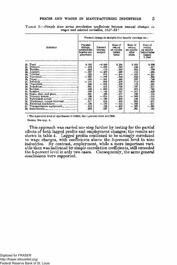
Table 3.— Simple time series correlation coefficients between annual changes in wages and selected variables, 1947-58 1
PRICES AND WAGES IN MANUFACTURING INDUSTRIES 5
Peroent change in straight-time hourly earnings on—
IndustryPercent change,
production worker employment
Percentchange,output
Rate of return
on equity before taxes
Rate of return
on equity after taxes
Rate of return
on equity before taxes
lagged 1 year
20. Food....................................................... 0.165 -0.638 0.234 0.353 0.80521. Tobacco____________________________ -.476 -.099 .040 .168 .01722. Textiles____________________________ .408 .173 .848 .835 .70923. Apparel..................... ...................... ...... -.027 -.409 .236 .122 .39524. Lumber_______________ ___ ____ ____ .252 .012 -.200 -.322 —.20125. Furniture_______ ______ ____________ -.050 -.290 .643 .533 .80526. Paper.................. .................................... .049 -.344 .463 .529 .74927. Printing_______________ ____ ________ —.170 .098 .276 .712 .87028. Chemicals_____________ ____________ .266 -.005 .206 .178 .28729. Petroleum............... .............................. .681 .210 .706 .787 .31730. Rubber......................... ......................... .283 -.063 .540 .072 .79231. Leather___________________ _________ .192 -.145 .047 -.371 .43932. Stone, clay, and glass................. .......... .381 .139 .177 .188 .17333. Primary metals_________ _____ ______ .139 -.014 .204 -.009 .11034. Fabricated metals...................... ........... - . 131 - . 189 .399 .449 .71235. Machinery, except electrical__________ .317 .214 .595 .525 .67136. Electrical machinery________________ -.139 -.175 -.012 -.243 .61737. Transportation equipment___________ .218 .128 -.302 -.307 -.30138. Instruments............................................ .362 .237 .157 .281 .167
* The 6-percent level of significance is 0.6021; the 1-percent level is 0.7348. Source: See app. A.
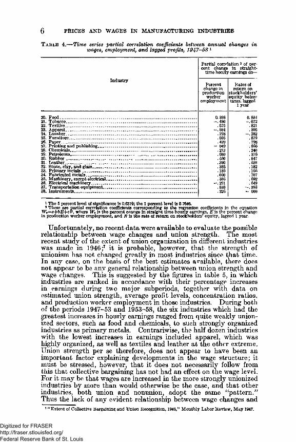
This approach was carried one step further by testing for the partial effects of both lagged profits and employment changes; the results are shown in table 4. Lagged profits continued to be strongly correlated to wage changes, with coefficients above the 5-percent level in nine industries. By contrast, employment, while a more important variable than was indicated by simple correlation coefficients, still exceeded the 5-percent level in only two cases. Consequently, the same general conclusions were supported.
Digitized for FRASER http://fraser.stlouisfed.org/ Federal Reserve Bank of St. Louis
6 PRICES AND WAGES IN MANUFACTURING INDUSTRIES
Table 4.— Time series 'partial correlation coefficients between annual changes in wages, employment, and lagged profits, 1947-58 1
Partial correlation2 of percent change in straight-
time hourly earnings on—Industry
Percent change in
production worker
employment
Rates of return on
stockholders’ equity before taxes, lagged
1 year
20. Food................................................................................................................ 0.398 0.83421. Tobacco___________________________________________________________ —.480 —.07222. Textiles _ _ _ __ _ _ __ .675 .82123. Apparel........... ........................................................................................... .24. Lumber___________________________________________________________
-.034.228
.395—.282
25. Furniture.......................... ........... .................................. ............ . ........... . .595 .87926. Paper.____ _______________ ______ ___ ____ _________________________ .420 .79827. Printing and publishing__ ____ _____________________________________ - 049 .86628. Chemicals................................................................................... ................ .213 .24029. Petroleum. .................................................. ......................... .......... ............. .680 .31630. Rubber........................................................................................................... .550 .84731. Leather__________________ ______ __________________________________ .390 .53832. Stone, clay, and glass_______________________________________________ .385 . 18233. Primary metals____________________________________________________ .186 .16634. Fabricated metals__________________________________________________ .050 .70735. Machinery, except electrical_________________________________________ .386 .69236. Electrical machinery_______________________________________________ -.291 .64937. Transportation equipment__________________________________________ .338 —.39338. Instruments_______________________________________________________ .326 - 008
1 The 5 percent level of significance is 0.6319; the 1 percent level is 0.7646.2 These are partial correlation coefficients corresponding to the regression coefficients in the equation
W,=a-)rbE+cF, where W, is the percent cnange in straight time hourly earnings, E is the percent change in production worker employment, and R is the rate of return on stockholders’ equity, lagged 1 year.
Unfortunately, no recent data were available to evaluate the possible relationship between wage changes and union strength. The most recent study of the extent of union organization in different industries was made in 1946 ;7 it is probable, however, that the strength of unionism has not changed greatly in most industries since ttiat time. In any case, on the basis of the best estimates available, there does not appear to be any general relationship between union strength and wage changes. This is suggested by the figures in table 5, in which industries are ranked in accordance with their percentage increases in earnings during two major subperiods, together with data on estimated union strength, average profit levels, concentration ratios, and production worker employment in those industries. During both of the periods 1947-53 and 1953-58, the six industries which had the greatest increases in hourly earnings ranged from quite weakly unionized sectors, such as food and chemicals, to such strongly organized industries as primary metals. Contrariwise, the half dozen industries with the lowest increases in earnings included apparel, which was highly organized, as well as textiles and leather at the other extreme. Union strength per se therefore, does not appear to have been an important factor explaining developments in the wage structure; it must be stressed, however, that it does not necessarily follow from this that collective bargaining has not had an effect on the wage level. For it may be that wages are increased in the more strongly unionized industries by more than would otherwise be the case, and that other industries, both union and nonunion, adopt the same “ pattern.” Thus the lack of any evident relationship between wage changes and
7 “ Extent of Collective Bargaining and Union Recognition, 1946,” Monthly Labor Review, May 1947.
Digitized for FRASER http://fraser.stlouisfed.org/ Federal Reserve Bank of St. Louis
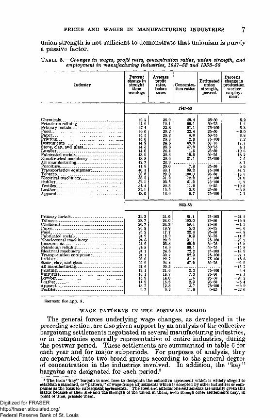
union strength is not sufficient to demonstrate that unionism is purely a passive factor.Table 5.— Changes in wages, profit rates, concentration ratios, union strength, and
employment in manufacturing industries, 1947-58 and 1953-58
PRICES AND WAGES IN MANUFACTURING INDUSTRIES 7
IndustryPercent
change in straight
time
Averageprofitrates,beforetaxes
Concentration ratios
Estimatedunion
strength,percent
Percent change in
production worker employ
ment
1947-63
Chemicals______________Petroleum refining.............Primary metals___ ______Food___________________Paper...........................—Printing.......... ...................Instruments_____________Stone, clay, and glass........Lumber......... ...................Fabricated metals....... ......Nonelectrical machinery ...All manufacturing....... ......Furniture_______________Transportation equipmentTobacco________________Electrical machinery.........Rubber______ ___________Textiles_________________Leather____ _____ ___ ___Apparel______ __________
49.2 26.0 59.4 25-50 5.247.6 1I 19.1 99.1 50-75 1.447.4 2 2 . 8 81.1 75-100 5.346.0 2 0 . 2 22.4 25-50 - 6 . 045.5 26.2 5.0 50-75 8 . 845.0 23.3 2.3 75-100 7.244.9 24.6 69.9 50-75 17.744.3 26.6 57.9 50-75 4.144.0 24.4 1.5 25-50 - 10 . 043.9 26.3 19.3 50-75 13.243.8 26.6 31.1 75-100 7. 542.7 23.9 8 .141.9 26.0 7.3 25-50 6 . 640.1 33.1 83.2 75-100 47.238.6 2 0 . 0 1 0 0 .0 25-50 -13 .538.2 31.2 72.2 75-100 31.037.5 25.5 51.2 75-100 0 . 231.4 20.3 11.9 0-25 - 1 0 . 831.1 15.5 2.3 25-50 - 6 .818.0 13.6 5.7 75-100 7.1
1953-58
Primary metals........... ......Tobacco________________Chemicals_______________Paper___________________Food___________________Fabricated metals_______Nonelectrical machinery....Instruments_____________Petroleum refining_______Electrical machinery_____Transportation equipmentRubber________ _________Stone, clay, and glass____All manufacturing_______Printing_________________Furniture--------- -------------Lumber_______ ____ ____Leather_________________Apparel_________________Textiles------ -------------------
31.28.26.26.25.24.24.24.24.24.24.23.22.21.18.16.15.14.13.
21.024.024.319.917.718.920.923.814.924.630.722.724.4 20.3 21.618.714.0 15.612.8 9.2
81.1100.059.4 5.0
22.4 19.331.169.999.172.282.3 51.257.9
2.37.3 1.52.3 5.7
11.9
75-10025-5025-5050-7525-5050-7575-10050-7550-7575-10075-10075-10050-75
75-10025-5025-5025-5075-1000-25
-21.2 -15 .9 -7 .3 -0.6 -8 .9
-14 .5 -20.2 -15 .8 -15.8 -18 .9 -27.1 -15 .6 -9 .2
-15.7 6.4
-7 .1 -20.2 -8 .4 -6 .9 -22.0
Sources: See app. A.
W A G E P A T T E R N S IN T H E P O S T W A R PERIOD
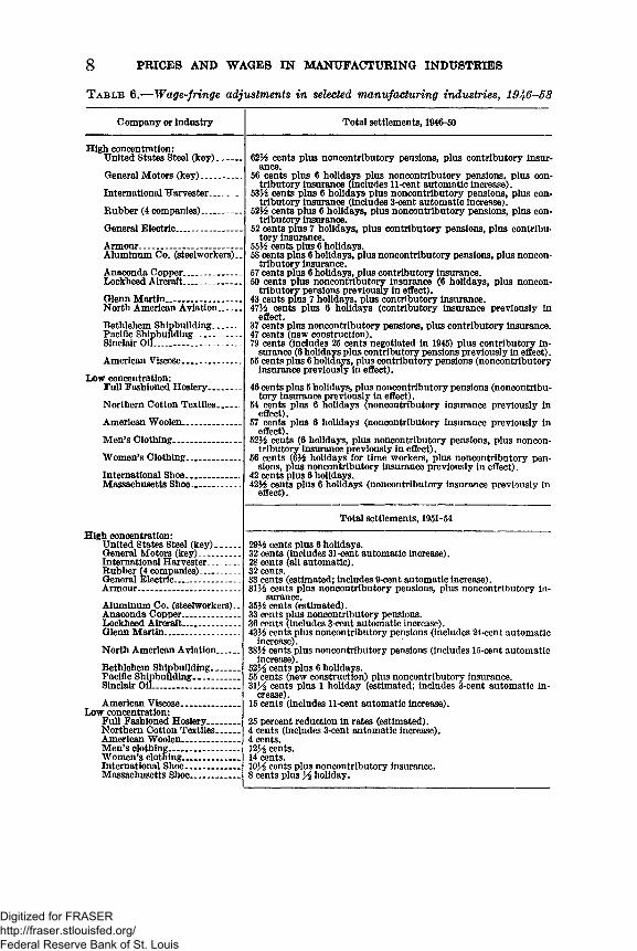
The general forces underlying wage changes, as developed in the preceding section, are also given support by an analysis of the collective bargaining settlements negotiated in several manufacturing industries, or in companies generally representative of entire industries, during the postwar period. These settlements are summarized in table 6 for each year and for major subperiods. For purposes of analysis, they are separated into two broad groups according to the general degree of concentration in the industries involved. In addition, the “key” bargains are designated for each period.8
8 The term “ key” bargain is used here to designate the collective agreement which is widely alleged to establish a standard, or “ pattern,” of wage-fringe adjustments which is accepted by other industries or companies as the basis for subsequent agreements. The steel and automobile settlements are usually given this status because of their size and the strength of the union in them, even though other settlements may, in point of time, precede them.
Digitized for FRASER http://fraser.stlouisfed.org/ Federal Reserve Bank of St. Louis
8 PRICES AND WAGES IN MANUFACTURING INDUSTRIES
T a b le 6.— Wage-fringe adjustments in selected manufacturing industries, 1946-58
Company or industry Total settlements, 1946-50
High concentration:United States Steel (key) _General Motors (key)— . International Harvester.. Rubber (4 companies)— . General Electric........Armour.....................................Aluminum Co. (steelworkers).Anaconda Copper.. Lockheed Aircraft..Glenn Martin.....................North American Aviation..Bethlehem Shi] Pacific Sinclair
lem Shipbuilding.Shipbuilding____rOil.......- ........—
American Viscose.Low concentration:
Full Fashioned Hosiery-Northern Cotton Textiles.American Woolen..............
Men’s Clothing.................Women’s Clothing_______International Shoe___Massachusetts Shoe...
High concentration:United States Steel (key)____General Motors (key)-...........International Harvester______Rubber (4 companies)....... ......General Electric...................Armour......................................
Aluminum Co. (steelworkers)Anaconda Copper....................Lockheed Aircraft.....................Glenn Martin.................... ........
North American Aviation___
Bethlehem Shipbuilding........ .Pacific Shipbuilding. ............. .Sinclair Oil................................ .
American Viscose......................Low concentration:
Full Fashioned Hosiery...........Northern Cotton Textiles____American Woolen.................... .Men's clothing............. ........... .Women’s clothing.................... .International Shoe................... .Massachusetts Shoe..................
62|4 cents plus noncontributory pensions, plus contributory insurance.
56 cents plus 6 holidays plus noncontributory pensions, plus contributory insurance (includes 11-cent automatic increase).
53H cents plus 6 holidays plus noncontributory pensions, plus contributory insurance (includes 3-cent automatic increase).
52J4 cents plus 6 holidays, plus noncontributory pensions, plus contributory insurance.
52 cents plus 7 holidays, plus contributory pensions, plus contributory insurance.
55H cents plus 6 holidays.58 cents plus 6 holidays, plus noncontributory pensions, plus noncon
tributory insurance.57 cents plus 6 holidays, plus contributory insurance.50 cents plus noncontributory insurance (6 holidays, plus noncon
tributory pensions previously in effect).43 cents plus 7 holidays, plus contributory insurance.47H cents plus 6 holidays (contributory insurance previously in
effect.37 cents plus noncontributory pensions, plus contributory insurance.47 cents (new construction).79 cents (includes 25 cents negotiated in 1945) plus contributory in
surance (6 holidays plus contributory pensions previously in effect).55 cents plus 6 holidays, plus contributory pensions (noncontributory
insurance previously in effect).46 cents plus 5 holidays, plus noncontributory pensions (noncontribu
tory insurance previously in effect).54 cents plus 6 holidays (noncontributory insurance previously in
effect).57 cents plus 6 holidays (noncontributory insurance previously in
effect).52H cents (6 holidays, plus noncontributory pensions, plus noncon
tributory insurance previously in effect).56 cents (6^ holidays for time workers, plus noncontributory pen
sions, plus noncontributory insurance previously in effect).42 cents plus 6 holidays.42H cents plus 6 holidays (noncontributory insurance previously in
effect).
Total settlements, 1951-54
29H cents plus 6 holidays.32 cents (includes 31-cent automatic increase).28 cents (all automatic).32 cents.33 cents (estimated; includes 9-cent automatic increase).31H cents plus noncontributory pensions, plus noncontributory in
surance.35H cents (estimated).33 cents plus noncontributory pensions.36 cents (includes 3-cent automatic increase).43J4 cents plus noncontributory pensions (includes 24-cent automatic
increase).38H cents plus noncontributory pensions (includes 15-cent automatic
increase).523 £ cents plus 6 holidays.55 cents (new construction) plus noncontributory insurance.Zl% cents plus 1 holiday (estimated; includes 3-cent automatic in
crease).15 cents (includes 11-cent automatic increase).25 percent reduction in rates (estimated).4 cents (includes 3-cent automatic increase).4 cents.12J4 cents.14 cents.10K cents plus noncontributory insurance.8 cents plus ]4 holiday.
Digitized for FRASER http://fraser.stlouisfed.org/ Federal Reserve Bank of St. Louis
PRICES AND WAGES IN MANUFACTURING INDUSTRIES
T a b le 6.— Wage-fringe adjustments in selected manufacturing industries,1946-58— Continued
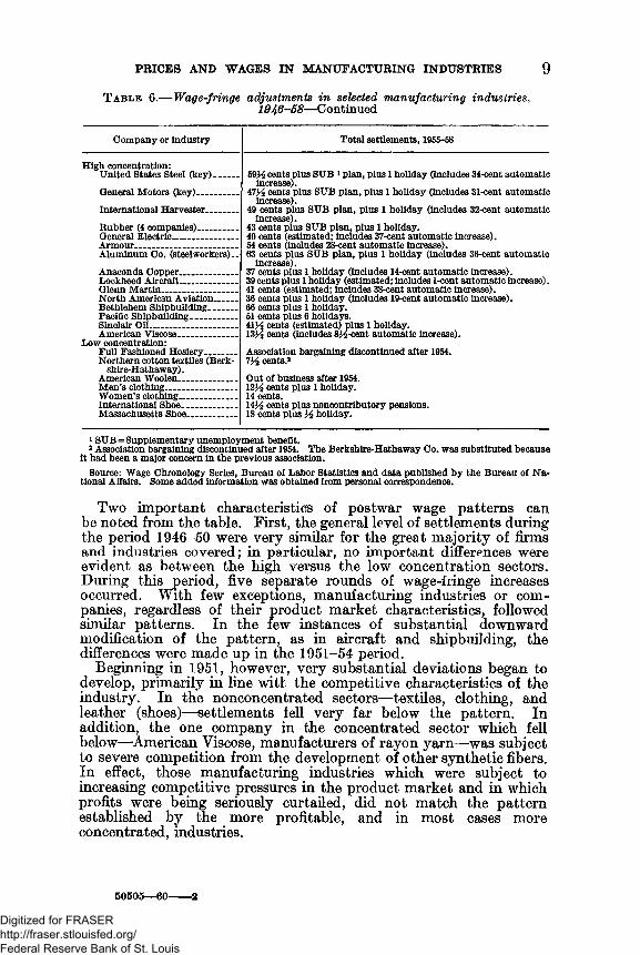
Company or industry Total settlements, 1955-58
High concentration:United States Steel (key).General Motors (key)__International Harvester..Rubber (4 companies).............General Electric......................Armour—.................................Aluminum Co. (steelworkers).Anaconda Copper....................Lockheed Aircraft...................Glenn Martin..........................North American Aviation.......Bethlehem Shipbuilding____Pacific Shipbuilding..............Sinclair Oil..............................American Viscose....................Low concentration:Full Fashioned Hosiery.......... .Northern cotton textiles (Berkshire-Hathaway) .American Woolen....................Men’s clothing....... ................. .Women’s clothing....................International Shoe..................Massachusetts Shoe..................
5 9 cents plus SUB 1 plan, plus 1 holiday (includes 34-cent automatic increase).473 cents plus SUB plan, plus 1 holiday (includes 31-cent automatic increase).49 cents plus SUB plan, plus 1 holiday (includes 32-cent automatic increase).43 cents plus SUB plan, plus 1 holiday.40 cents (estimated; includes 37-cent automatic increase).54 cents (includes 28-cent automatic increase).63 cents plus SUB plan, plus 1 holiday (includes 36-cent automatic increase).37 cents plus 1 holiday (includes 14-cent automatic increase).39 cents plus 1 holiday (estimated; includes 1-cent automatic increase).41 cents (estimated; includes 38-cent automatic increase).36 cents plus 1 holiday (includes 19-cent automatic increase).66 cents plus 1 holiday.51 cents plus 6 holidays.41H cents (estimated) plus 1 holiday.13M cents (includes 834-cent automatic increase).Association bargaining discontinued after 1954. cents.2Out of business after 1954.12^ cents plus 1 holiday.14 cents.143 cents plus noncontributory pensions.18 cents plus XA holiday.
1 SUB= Supplementary unemployment benefit.* Association bargaining discontinued after 1954. The Berkshire-Hathaway Co. was substituted because it had been a major concern in the previous association.Source: Wage Chronology Series, Bureau of Labor Statistics and data published by the Bureau of National Affairs. Some added information was obtained from personal correspondence.
Two important characteristics of postwar wage patterns can be noted from the table. First, the general level of settlements during the period 1946-50 were very similar for the great majority of firms and industries covered; in particular, no important differences were evident as between the high versus the low concentration sectors. During this period, five separate rounds of wage-fringe increases occurred. With few exceptions, manufacturing industries or companies, regardless of their product market characteristics, followed similar patterns. In the few instances of substantial downward modification of the pattern, as in aircraft and shipbuilding, the differences were made up in the 1951-54 period.
Beginning in 1951, however, very substantial deviations began to develop, primarily in line with the competitive characteristics of the industry. In the nonconcentrated sectors— textiles, clothing, and leather (shoes)— settlements fell very far below the pattern. In addition, the one company in the concentrated sector which fell below—American Viscose, manufacturers of rayon yarn—was subject to severe competition from the development of other synthetic fibers. In effect, those manufacturing industries which were subject to increasing competitive pressures in the product market and in which profits were being seriously curtailed, did not match the pattern established by the more profitable, and in most cases more concentrated, industries.
50505— 60-----2
Digitized for FRASER http://fraser.stlouisfed.org/ Federal Reserve Bank of St. Louis
This general situation continued through 1955-58. The textile and clothing industries, including American Viscose, and the shoe lirms continued to reach agreements far below the level set in the better situated industries. Within the latter, more diversification also developed, although the bulk of settlements ranged between 40 and 50 cents per hour. The major exceptions were in industries organized by the steel union— steel, aluminum, and Atlantic coast shipbuilding (Bethlehem Steel C o.); in these sectors, wage increases were 59K, 63, and 66 cents, respectively (plus fringes), over the 4-year period.
The second point to be noted from the data is the increasing importance of automatic wage changes, incorporated into long-term contracts in the form of cost-of-living adjustments and annual improvement factors. During the 1946-50 period, this approach was introduced by General Motors, but was rarely followed elsewhere. In 1951-54, however, largely as a result of the sharp rise in the cost of living which accompanied the outbreak of the Korean war in 1950, the annual improvement factor-cost of living approach was adopted in automobiles, farm equipment, aircraft, electrical equipment, and a few others. The steel union, however, continued to follow the more traditional approach, as did several other leading companies and unions.
During 1955-58, however, most of the latter group also went over to automatic adjustments. As a result, virtually every strongly unionized company in the concentrated sectors listed in table 6 had negotiated long-term contracts in 1955 and 1956, providing for automatic annual wage increases plus automatic costs-of-living adjustments through 1957, 1958, and, in some cases, 1959. The only exceptions were rubber, shipbuilding, and oil (Sinclair). On the other hand, none of the low concentration sectors followed this policy after 1955.
The sequence of wage developments during the 1955-58 period is also of very considerable interest. In the summer of 1955, the major “ key” bargain was negotiated in the automobile industry, in which sales and profits were at record or near record levels. The contract extended for 3 years to mid-1958, and included an annual improvement factor of approximately 6 cents per hour, a cost-of-living clause, and additional fringes estimated to be worth approximately 12 cents per bour. Shortly thereafter, the steel industry negotiated a straight wage increase of 15 cents, under a wage reopener clause, in a contract which expired in 1956. Output and profits in steel had also risen sharply from the 1954 recession low; the relevant data for both the automobile and steel industries are shown in table 7. Before the year was out, the leading firms in several other major industries in which market conditions and profits were adequate had negotiated similar contracts, with many adopting the 3-year approach of the automobile industry.
10 PRICES AND WAGES IN MANUFACTURING INDUSTRIES
Digitized for FRASER http://fraser.stlouisfed.org/ Federal Reserve Bank of St. Louis
PRICES AND WAGES IN MANUFACTURING INDUSTRIES 11
T a b le 7.— Basic trends in the steel and automobile industries, 1947-58
YearProfits before Profits aftertaxes on taxes on Profits before Outputequity equity taxes as per (1947-49=(percent) (percent) cent of sales 100)
Production worker employment (1947-49= 100)
IRON AND STEEL1947.1948..1949..1950..1951.. 1952.1953..1954..1955..1956..1957.1958.
19.817.017.028.134.017.6 25.516.027.125.122.714.2
12.114.7 9.914.212.310.7 8.113.512.711.4 7.2
10.912.310.9 15.1 16.09.312.410.514.512.9 13.010.5
10110692118131117139109146143139105
101105931041109511097107104105
MOTOR VEHICLES1947.............................................. 27.9 15.6 10.4 95 1001948.............................................. 32.9 1&7 11.8 101 1011949.............................................. 35.8 20.9 13.2 104 981950.............................................. 51.8 24.6 17.1 132 1091951.............................................. 39.5 14.1 13.2 120 1101952.............................................. 36.8 13.6 12.6 102 1001953.............................................. 37.9 13.6 11.0 126 1191954.............................................. 29.4 13.9 10.8 109 971955.............................................. 46.1 21.1 15.1 153 1161956.............................................. 27.1 13.0 10.8 125 1001957.............................................. 28.1 14.0 10.8 128 981958.............................................. 14.4 8.1 7.0 99 74
Sources: See app. A, The output index for “Iron and Steel” is the Federal Reserve Board index of industrial production, with 1947 weights.In mid-1956, the “ key” bargain open for negotiation was in steel.
Both production and profits were at about their 1955 levels, a major investment boom was developing in plant and equipment, and the precedent set by the previous year’s settlements in automobiles and other industries was strong. The result was an extremely favorable contract for the steelworkers—a 3-year contract extending into 1959, including a 9-cent annual improvement factor, automatic cost-of- living adjustments, and major fringe benefits. Similarly, favorable long-term contracts were signed in the aluminum industry; in most others, the terms were somewhat less liberal, but also involved longterm commitments to annual wage increases.
The results of these two major “patterns,” established in the automobile and steel industries during the period of high output and profits, continued to be felt throughout the declining years of 1957 and 1958. In both of these years, despite marked declines in output and employment throughout the economy, wage increases were automatic in several major manufacturing industries. Further, the widespread use of cost-of-living escalators magnified the effects of quite
Digitized for FRASER http://fraser.stlouisfed.org/ Federal Reserve Bank of St. Louis
small (originating) increases in the Consumer Price Index. The automobile contract, which terminated in the midst of the sharp recession of 1958, was again renewed for a 3-year period, and again included an automatic annual improvement factor of 2}{ percent per year (about 7 cents) plus cost-of-living adjustments. Thus the recession did not appear to have had any appreciable effect on the annual rate of increase in negotiated rates; the direct costs of additional fringe benefits negotiated in the 1958 automobile contract, however, were very low. And in 1959, the steel contract was again being negotiated in the context of a developing boom.
The probability that the rate of increase in wages after 1958 has not been appreciably affected by the 3-year automobile contract is given added support by a comparison of the wage-fringe increases negotiated during the first 6 months of 1959 as compared to the same period in 1955. These periods were generally comparable, since they both represented approximately the same phase of sharp recovery from previous recessions. From December 1954 to June 1955, unemployment declined from 5.0 to 4.1 percent, seasonally adjusted; in the same period, December 1958 to June 1959, the rate fell from 6.1 to 4.9 percent.
NEGOTIATED SETTLEMENTS, FIRST SIX MONTHS 1955 AND 1959
12 PRICES AND WAGES IN MANUFACTURING INDUSTRIES
Thousonds of workers
Source: Bureau of Labor Statistics.
The above chart relates to settlements involving 1,000 or more workers concluded during the 6-month period. It includes all wage changes negotiated during the January-June period that are scheduled to go into effect during the contract year—i.e., the 12-month period following the effective date of the agreement. In summarizing percentage increases, it has been necessary to estimate
Digitized for FRASER http://fraser.stlouisfed.org/ Federal Reserve Bank of St. Louis
their value in terms of cents on the basis of available information on wage levels in the industry.
This chart excludes—Settlements involving fewer than 1,000 workers.Settlements in construction, the service trades, finance, and government.Instances in which contract reopening privileges were not exercised.Wage increases and changes in supplementary practices that went into
effect during the period but that were negotiated earlier—for example, deferred wage increases, cost-of-living adjustments, or annual improvement factor increases.
Chart 1 provides a comparison of the number of employees covered by negotiated contracts who received wage increases within specified ranges in the first 6 months of 1955 and 1959. In 1955, 72 percent of employees received wage increases of 5 to 11 cents, compared to only 60 percent in early 1959. However, a full 30 percent received more than 11 cents in 1959, contrasted to only 8 percent in 1955; contrariwise, 15 percent received less than 5 cents in 1955 compared to 8 percent in 1959. An estimate of the weighted average of wage increases for 1955 was 7.6 cents; in 1959, 9.2 cents. This increase of about 20 percent approximates the rise in hourly earnings from 1955 to 1959; relatively, therefore, the 1959 increase was no greater than 1955. On the other hand, the rate of unemployment was almost one percentage point greater in the first 6 months of 1959 as compared to 1955. And finally, 69 percent of the 1959 settlements also liberalized one or more fringe benefits as contrasted to 60 percent in the first 6 months of 1955, although the costs of the 1959 fringes may well have been below those of 1955. The weight of evidence, however, indicates that the rate of advance in wage-fringe costs has not been slower during the 1959 upswing.
One final possible qualification should be noted. The data on which these comparisons are based excludes contracts which contained reopening clauses that were not utilized—that is, contracts in which no increases occurred because the union chose not to request one. They also exclude several types of settlements noted in the chart. It is doubtful that this would affect the data in any important way.
III. T h e M o v e m e n t o f M a n u fa c tu r in g P r ic e s
An analysis similar to that applied to wage movements was also carried out for price movements in 16 two-digit manufacturing industries. Since the Bureau of Labor Statistics does not compute wholesale price indexes on a basis consistent with most two-digit classifications, it was necessary to construct such indexes by recombining various subgroups of the wholesale price index. The sources and methods used are described in appendix A. The resulting price indexes are shown in table 8 9; in all, they account for close to 80 percent of the weights in the entire wholesale price index, and for approximately 95 percent of the total weight in the “all manufactures” index. The major additional items included in the entire wholesale price index are, of course, farm products.
8 Only 16 industrial sectors are represented because of lack of adequate price data for the remaining 3— printing and publishing, transportation equipment, and instruments. Wherever feasible in the following discussion, price and other data for the three-digit industry, motor vehicles, is used in place of transportation equipment. All of the statistical tests, however, are based only upon the 16 two-digit sectors.
PRICES AND WAGES IN MANUFACTURING INDUSTRIES 13
Digitized for FRASER http://fraser.stlouisfed.org/ Federal Reserve Bank of St. Louis
T a b le 8.— Wholesale price indexes in manufacturing industries, 1 9 4 7 -5 8 1[1947-49*100]
Industry 1954weight
1947 1948 1949 1950 1951 1952 1953 1954 1955 1956 1957 1958 Percentincrease
Primary metals_______ . ________. . . . . . . . . ______—____. . . . 7.13 90.4 102.8 106.8 111.7 123.8 125.1 132.3 136.1 145.0 157.8 163.0 164.2 81.6N onelectrical machinery... . . . . . . . . . . . . . . . . . . . . . . . . . . . . . . 7.82 92.4 101.1 106.6 110.2 122.5 123.1 125.7 127.8 133.3 144.2 153.5 157.1 70.0Stone, clay, glass___ 2.15 92.7 101.1 105.5 109.3 117.3 118.1 123.6 127.4 131.5 139.0 144.7 149.5 61.3Fabricated metals_ 5.28 90.8 102.5 106.7 110.4 121.6 120.6 122.4 124.0 127.8 136.0 141.8 142.6 57.0Motor vehicles and equipment 5.55 91.3 100.8 107.9 107.2 112.9 119.6 118.9 119.3 122.9 129.8 135.4 139.7 53.0Rubber products. 1.35 98.0 101.8 100.2 112.0 132.5 128.4 125.7 127.7 140.2 145.6 146.5 148.2 51.2Electrical m a c h i n e r y . . . . * . . . . . . . . . . . . . . . . . . . . . . . . . . . . . . . . 7.11 96.3 101.5 102.2 103.7 116.2 117.0 120.4 120.3 123.4 133.2 139.7 140.7 46.1Furniture____ ___ 1.30 95.3 102.3 102.3 106.5 118.7 115.9 117.1 117.2 119.2 125.6 130.6 132.1 38.6Tobacco products___ _____________. . . . . __________________ .97 95.6 99.6 104.9 107.0 110.4 111.3 119.1 120.7 120.8 121.0 126.4 131.0 37.0paper and allied_. . . . . . . . . . . . . . . . . . . . . . . . . . . . . . . . . . . . . . . 5.17 98.6 102.9 98.5 100.9 119.6 116.5 116.1 116.3 119.3 127.2 129.6 131.0 32.9All m a n u f a c t u r i n g . . . . . . . . . . . . . . . . . . . . . . . . . . . . . . . . . . . . . . . 82.95 95.9 103.8 100.3 104.1 115.5 112.9 112.8 113.7 115.0 119.5 123.2 124.5 29.8Petroleum products......... ............. . » .r- 4.24 89.6 112.1 98.3 111.0 109.4 111.2 111.9 109.0 111.2 117.5 125.8 114.8 28.1Lumber p r o d u c t s . . . . . . . . . . . . . . . . . . . . . . . . . . . . . . . . . . . . . . . . 2.97 93.7 107.2 99.2 113.9 123.9 120.3 120.2 118.0 123.6 125.4 119.0 117.7 25.6Food products..*____ ___________________________________ 12.73 98.2 106.1 95.7 99.8 111.4 108.8 104.6 105.3 101.7 101.7 105.6 110.9 12.9Leather products__ . . . . . . . . . . . . . . . . . . 1.27 99.5 102.1 98.4 104.9 120.5 103.8 104.3 101.6 101.4 107.4 108.0 109.0 9.5Chemicals___ _______________________________. . . _________ 5.83 101.4 103.8 94.8 96.3 110.0 104.5 103.6 107.0 106.6 107.2 109.5 110.4 8.9Apparel_______. . . . . . . . . . . . . . . . . . . . . . . . . . . . . . . . . . . . . . . . . . 3.22 100.7 103.2 96.1 96.7 104.4 101.2 100.6 100.1 100.3 101.7 101.8 101.6 .9Textile products____________ ____________________________ 3.18 99.2 105.9 94.9 101.2 115.9 98.9 95.4 91.8 92.2 91.7 91.5 88.0 -11 .3
* Printing and publishing, transportation equipment, and instruments are omitted because of lack of data.* Motor vehicles and equipment is included in place of transportation equipment.Sources: See app. A.
PRICES AND
WAGES
IN M
ANU
FACTUR
ING
IN
DU
STR
IES
Digitized for FRASER http://fraser.stlouisfed.org/ Federal Reserve Bank of St. Louis
A complete year-to-year cross-section analysis, relating the percentage change in price to several variables, was conducted. The simple correlation coefficients for several of the more important possible relationships are listed in table 9. In addition, the complete matrix of all possible simple correlation coefficients is provided in appendix B.Table 9.— Simple cross-section correlation coefficients between price changes and
selected variables in 16 manufacturing industries, 1947-58 1
PRICES AND WAGES IN MANUFACTURING INDUSTRIES 15
Percentage change in wholesale price index on—
YearGrosshourly
earnings
Productivity per production worker man-hour
OutputAverageprofitsbeforetaxes
Averageprofitsaftertaxes
Concentration ratios
1947-48............................... 0.093 0.024 0.375 0.339 0.560 0.3291948-49............................... .214 .328 -.416 .439 .335 .2871949-50............................... —.055 .170 .073 —.041 .113 —.0191950-51 ............................. .101 —.415 - . 199 .294 —.066 —.5261951-52............................... .375 .035 - . 065 .536 .624 .5811952-53............................... .546 - . 171 .176 .490 .432 .5951953-54............................... .620 -.215 -.247 .715 .505 .3871954-55............................... .551 —.201 .587 .448 .395 .1961955-56............................... —.098 -.418 .283 .404 .442 .1931956-57............................... .551 - . 100 .397 .585 .711 .6171957-58 ............................. .308 .329 .115 .629 .276 -.114
i The 5-percent level of significance is 0.4973. The 1-percent level is 0.6226. Source: See apps. A and B.
A number of interesting points are indicated. Perhaps of greatest importance is the lack of any evident relationship between changes in prices and changes in output, at least up to 1954. After 1954, the correlation became weakly positive, except for the one year of sharp recovery, 1954-55, when a significant relationship appeared.
The remaining findings may be briefly summarized as follows:1. Changes in prices were not strongly related to changes in produc
tivity per production worker man-hour. It is of some interest, however, that several negative correlations appeared, indicating that lower price increases were often associated with greater increases in productivity.
2. Price changes were unrelated to changes in gross hourly earnings during the early part of the period up to 1951-52. After that point, however, the correlation became very much stronger.
3. Price adjustments were clearly related to profit levels throughout most of the postwar period; the relationship was strongest, however, after 1951.
4. The relationship of price changes to concentration ratios was quite irregular. Up to 1951, it was low or negative; in fact, the strong negative correlation in 1950-51 suggests that prices in nonconcentrated industries rose more than in concentrated. From 1951 to 1957, however, the coefficient was consistently positive, though the strength of the relationship varied considerably. And finally, the correlation became weakly negative in the 1957-58 recession.10
10 The first three of these results, relating to output, productivity, and earnings, were also found by Conrad, op. cit. Using both simple and multiple regression analysis to test price changes against changes in wages, output, productivity, and employment, he concluded that “only the price-wage relationship and the price- employment change relationship approach economic significance”; his data show a much lower partial correlation coefficient for the latter relationship, however. His analysis included 61 three-digit industries.
Digitized for FRASER http://fraser.stlouisfed.org/ Federal Reserve Bank of St. Louis
A closer evaluation of the relationship of prices to output and wages was obtained by a multiple cross-section regression analysis covering the two subperiods 1947-53 and 1953-58. The percentage change in the wholesale price index was tested against (1) the percentage change in output and (2) the percentage change in direct labor costs per unit of output per total worker man-hour. The latter variable thus takes account of the effects of productivity on labor costs as well. The results are shown in table 10. Output was not a significant variable during either subperiod (after taking account of changes in unit direct labor costs); on the other hand, direct labor costs were highly correlated with price changes during the 1953- 58 period, but much less strongly so from 1947 to 1953. In general, these findings are consistent with those indicated by the simple correlation analysis.
16 PRICES AND WAGES IN MANUFACTURING INDUSTRIES
Table 10.— Cross-section regression equations: Prices
Independent variableRegressioncoefficient Partialcorrelation
coefficientBeta coeffi
cient Standard error of beta coefficient
1947-53:Percent change:Output ______________________ 0.1891 0.2516 0.2365 0.2522Direct labor costs per unit of output per total worker man-hour_______ .4982 .3730 .3661 .25221953-58:Percent change:Output ______________________ .2395 .3681 .3261 .2284.2284
Direct labor costs per unit of output per total worker man-hour________ *.9367 ».7630 .9724
Regression constants:1947-53........ ......................................................... ............................................... ....................... 6.841953-58.................................................................. ........................... .......................................... 3.76Multiple correlation coefficient:1947-53....................................................................... ............................... .................................. R « .42091953-58........ ..........................- -------------------------- ------------------------------------- --------- --------- R =1.7916Coefficient of multiple determination:1947-53........................................................................................... - ...................... ......... - ........i?2= .17721953-58.........................................................................- ............................. - ..........................— R *-». 6266
Degrees of freedom................. ..... ................................................................... .......... N-3=13i Significant at the 5 percent level.
Similar relationships were shown by time series analyses, although the small number of observations and the major structural shifts which occurred in the economy during the 1947-58 period limit the usefulness of time series for this purpose. In table 11, the simple correlation coefficients are given for each two-digit industry, indicating the relationship between price changes and several other variables from 1947 to 1958. Table 12 summarizes the results of a multiple regression analysis, relating the percent change in prices to (1) the percent change in output, and (2) the percent change in gross hourly earnings. In both cases, the price-output relationship was very weak, while the price-gross hourly wage relationship was strong. In 8 of the 16 industries, the price-wage correlation was significant at the 5-percent level; in 2 more, it was close to that level of significance. In addition, the simple correlation coefficients between price changes and profit levels were at or close to 5-percent significance level in nine industries. Thus the time series data tend to corroborate the general results of the cross-section analysis.
Digitized for FRASER http://fraser.stlouisfed.org/ Federal Reserve Bank of St. Louis
Table 11.— Simple time series correlation coefficients between annual changes in prices and selected variables, 1947-58 1
PRICES AND WAGES IN MANUFACTURING INDUSTRIES 1 7
Percent change In wholesale price index on—
Industry Percent change:
Gross hourly earnings
Percentchange:Ouptut
Percent change:
Productivity per production worker man-hour
Rate of return on equity,
before taxes
20. Food__________ -_____ __________________ 0.490 -0.287 -0.517 0.15221. Tobacco____________ . . . . . . ______________ .132 -.117 .270 .03122. Textiles_______________________________. . .651 .413 -.683 .60823. A pparel._________ ___ _____________ ___ .816 —.028 —.232 .12624. Lumber________________________________ -.187 .780 .213 .91425. Furniture_______________________________ .655 -.065 -.414 .65526. Paper__________________________________ .497 .275 —.065 .77128. Chemicals______________________________ .378 .357 -.145 .59929. Petroleum______ _______________________ .565 .587 .476 .68530. Rubber _______________________________ .245 .543 -.562 .72431. Leather_________________________________ .574 -.318 -.270 -.01632. Stone, clay, and glass____________________ .826 .265 -.093 .22833. Primary metals_________________________ .692 .442 .062 .67534. Fabricated metals_________________. _____ .755 .159 -.053 .62035. Machinery, except electrical______________ .727 .419 -.545 .49536. Electrical machinery_____________________ .652 .236 -.498 .280
i The 5 percent level of significance is 0.6021- the 1 percent level is 0.7348. Sources: See app. A.
Table 12.— Time series partial correlation coefficients between annual changes in prices, output, and hourly earnings, 1847-58 1
IndustryPartial correlation2 of
percent change in price on—
Change in output
Change in gross hourly
earnings
20. Food________________________________________________________ _____ -0.037 0.41621. Tobacco_____________________________________________________ ____ _ —.114 .12922. Textiles______________________________________________________ _____ .290 .60423. Apparel ____—___________________________________ _______________ .202 .82524. Lumber___________________________________________________________ .807 —.37525. Furniture _______________________________________________________ —.006 .65326. Paper_____________________________________________________________ .331 .52328. Chemicals_______________________________________________________ .319 .34229. Petroleum_________________________________________________________ .534 .50830. Rubber_____________________________ -_____________________________ .501 .02731. Leather____________________________________________________________ —.277 .55832. Stone, clay, and glass_______________________________________________ —.081 .81333. Primary metals____________________________________________________ .238 .62334. Fabricated metals___ ______________________________________________ —. 108 .75135. Machinery, except electrical_________________________________________ —.138 .66336. Electrical machinery_______________________________________________ .276 .661
J The 5 percent level of significance is 0.6319; the 1 percent level is 0.7646.2 These are partial correlation coefficients corresponding to the regression coefficients in the equation
P =a+bO +cW o, where P is the percent change in wholesale price, O is the percent change in output, and Wq is the percent change in gross hourly earnings.
TR EN D S IN SPECIFIC M A N U FAC TU RIN G IN D U ST RIE S
On the basis of the data on prices, wages, productivity, and profits, indexes were computed for each two-digit industry for which data were available, reflecting trends in the wholesale price index, direct labor costs per unit of output per total worker man-hour, and returns to capital (profits before taxes plus depreciation and depletion charges) per dollar of sales. These indexes are described in appendix A. In order to compare the movements of each of these variables both within each industry and among industries, ratios were computed to show the trends of each variable in each two-digit industry relative
Digitized for FRASER http://fraser.stlouisfed.org/ Federal Reserve Bank of St. Louis
to the trend in manufacturing as a whole. The resulting ratios are included in appendix C.
While these indexes are probably indicative of general trends in manufacturing industries, their limitations should be carefully noted. It has already been pointed out that the scope and method of classifying these various series differ, depending largely upon the nature and availability of the data involved. Thus profits are on a corporate basis, earnings, employment, and output are on an establishment basis, and prices on a product basis. In addition, the series included are not exhaustive, i.e., they do not reflect all the costs (including profits) which go to make up the final price. In particular, no data are available on the costs of materials; also, indirect taxes may be an important element of price in a few instances, as in tobacco products. Finally, the indexes of direct labor costs per unit of output very probably understate the actual rate of increase in labor costs, since they are based on the trend in gross hourly earnings of production workers only; no figures are available to show average hourly labor costs of both production and nonproduction workers. The resulting indexes probably understate the rate of increase in labor costs because (1) the rate of increase of employment of nonproduction workers has considerably exceeded that of production workers; in fact, the total number of production workers employed in manufacturing in 1958 was considerably lower than in 1947, whereas employment of nonproduction workers had risen by over 50 percent, and (2) because the average level of hourly compensation for nonproduction workers very probably exceeded the average hourly earnings of production workers. Thus, the shift in “ employee mix” would result in a greater rate of increase in labor costs than would be reflected in the trend of earnings for production workers alone.
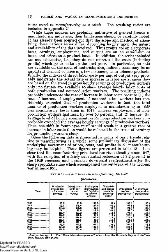
Since the following data is presented in terms of basic trends relative to manufacturing as a whole, some preliminary discussion of the underlying movement of prices, costs, and profits in all manufacturing may be helpful. These figures are presented in table 13. It is clear that the manufacturing price level has risen steadily since 1947, with the exception of a fairly substantial reduction of 3.2 percent in the 1949 recession and a smaller downward readjustment after the sharp speculative rise which accompanied the outbreak of the Korean war in mid-1951.
Table 13.— Basic trends in manufacturing, 1947-58
18 PRICES AND WAGES IN MANUFACTURING INDUSTRIES
[1947-49=100]
YearWholesale
price index: All manufactures
Direct labor costs per unit of output
Profits plus depreciation and depletion
as percent of sales
Materials and compo- ments for manufac
turing
Productionworker
employmentNonproduction worker employment
1947........................ 95.9 96.3 102.3 96.4 103.4 97.41948....................... 103.8 101.6 105.0 104.0 102.8 101.81949....................... 100.3 101.6 92.7 99.6 93.8 100.81950....................... 104.1 99.8 119.0 104.5 99.6 103.51951....................... 115.5 109.2 114.6 118.4 106.4 115.21952....................... 112.9 111.6 99.7 113.4 106.3 124.61953....................... 112.8 114.6 100.6 115.2 111.8 133.01954....................... 113.7 114.5 98.0 115.4 101.8 133.01955....................... 115.0 112.1 112.8 118.2 105.6 136.81956....................... 119.5 115.8 109.3 123.7 106.7 144.81957....................... 123.2 118.8 102.3 126.9 104.4 151.21958....................... 124.5 120.4 92.7 127.2 94.2 148.8
Sources: See app. A. The “ Materials and components” index is from the Economic Report of the Pres-dent, January 1959, p. 198.
Digitized for FRASER http://fraser.stlouisfed.org/ Federal Reserve Bank of St. Louis
PRICES AND WAGES IN MANUFACTURING INDUSTRIES 19
SOURCES A N D LIM ITA TIO N S OF DATA
During the early part of this period from 1947 to 1950, labor costs and profits all rose considerably. From 1950 to 1954, profit margins declined, then again rose sharply with the strong recovery of 1955. During the subsequent period to 1957, they declined moderately, then fell considerably in tne 1958 recession. By the end of the period (1956-58), the proportion of the sales dollar going into profits plus depreciation and depletion was at approximately the same level as in 1947-49. The pattern of movement, however, has been for gross margins to rise sharply at the beginning of boom periods and to recede gradually during the subsequent years of “ leveling off.”
The index of direct labor costs per unit of output has shown a continuing upward trend over the period, except for relatively small declines in 1950 and 1955, undoubtedly reflecting the increase in productivity which normally accompanies a strong upswing in output.11 Table 13 also shows the very considerable shift in employment toward nonproduction workers. It has already been noted that one probable result of this shift in employment patterns has been to raise the rate of increase in total labor costs per unit faster than is reflected in the index of unit direct labor costs. An additional implication of the rising importance of nonproduction worker employment is the fact that labor costs have become less responsive to cutbacks in production during recessions; this is clearly shown by the very much greater cutbacks in production worker than in nonproduction worker employment during the recessions of 1949, 1954, and 1958. By the same token, as Schultze has pointed out, one major reason for the rapid rise in labor costs per unit from 1955 to 1957 was the more than 10 percent increase in nonproduction worker employment as contrasted to the rise of only 3.5 percent in manufacturing production; the result, of course, was to hold down the rate of increase in productivity per total worker man-hour.12 One must presume, however, that in the long run, producers expect the shift in employee- mix to represent a profitable choice; in the 1955-58 period, however, it probably had a considerable adverse effect on unit labor costs and profit margins.
The data included in appendix C provide a basis for comparing the general trends of prices, wages, profits, and other variables over time, both within and between industries. In table 14, ratios of the specific industry indexes to the index of all manufacturing are shown for several important variables, as of 1957.13 The year 1957 is used in order to avoid the effects on the data of the 1958 recession. For purposes of analysis, the industries have also been classified according to the extent of concentration and the strength of unionization in each. It should be stressed, however, that these trends cannot be considered as anything more than suggestive; considerably more detailed studies would be required within each sector before a more
11 It must be stressed here that the trend indicated by the index of profits margins cannot be meaningfully compared to the trend indicated by the index of labor costs per unit of output, since the basis of computing the indexes is quite different. The index of profit margins is a measure of profits deflated by sales. The index of labor costs per unit, on the other hand, is a measure of direct labor costs deflated by man-hour productivity. The profits index reflects a percentage, whereas the labor cost index reflects an absolute amount.
12 See Charles L. Schultze, “ Recent Inflation in the United States,” Joint Economic Committee Study of Employment, Growth, and Price Levels, Study Paper No. 1.
is it should be noted that we are here comparing the ratios of indexes, rather than the indexes of each variable directly. Thus the problem cited in footnote 11 does not arise.
Digitized for FRASER http://fraser.stlouisfed.org/ Federal Reserve Bank of St. Louis
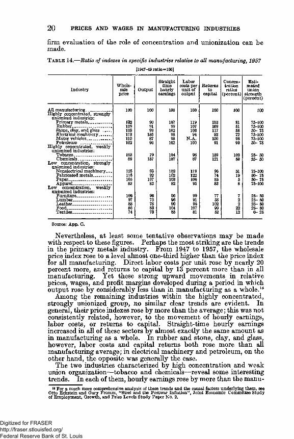
firm evaluation of the role of concentration and unionization can be made.T a b l e 14.— Ratio of indexes in specific industries relative to all manufacturing, 1957
20 PRICES AND WAGES IN MANUFACTURING INDUSTRIES
[1947-49 ratio ==100]
IndustryWhole
saleprice
OutputStraight
timehourly
earnings
Labor costs per unit of output
Returnsto
capital
Concentrationratios
(percent)
Estimatedunion
strength(percent)
All manufacturing- ................... 100 100 100 100 100 100 100Highly concentrated, strongly
unionized industries:Primary metals................... 132 90 107 119 113 81 75-100Rubber................................ 119 91 99 107 109 51 75-100Stone, clay, and glass.......... 118 99 102 103 117 58 50- 75Electrical machinery........... 113 135 98 94 92 72 75-100Motor vehicles..................... 110 87 98 N.A. 100 96 75-100Petroleum. .......................... 102 96 102 100 91 99 50- 75
Highly concentrated, weakly unionized industries:
Tobacco. ............................. 103 79 104 98 139 100 25- 50Chemicals .......................... 89 137 107 87 121 59 25- 50
Low concentration, strongly unionized industries:
Nonelectrical machinery.. . 125 93 102 119 96 31 75-100Fabricated metals............... 115 92 102 122 74 19 50- 75Paper................................... 105 107 103 106 83 5 50- 75Apparel................................ 83 82 82 95 83 8 75-100
Low concentration, weakly unionized industries:
Furniture............................. 106 96 96 99 77 7 25- 50Lumber................................ 97 75 96 91 58 2 25- 50Leather_________ ________ 88 78 90 96 102 2 25- 50Food______ _____________ 86 83 104 107 90 22 25- 50Textiles................................ 74 73 85 81 52 12 0- 25
Source: App. O.
Nevertheless, at least some tentative observations may be made with respect to these figures. Perhaps the most striking are the trends in the primary metals industry. From 1947 to 1957, the wholesale price index rose to a level almost one-third higher than the price index for all manufacturing. Direct labor costs per unit rose by nearly 20 percent more, and returns to capital by 13 percent more than in all manufacturing. Yet these strong upward movements in relative prices, wages, and profit margins developed during a period in which output rose by considerably less than in manufacturing as a whole.14
Among the remaining industries within the highly concentrated, strongly unionized group, no similar clear trends are evident. In general, their price indexes rose by more than the average; this was not consistently related, however, to the movement of hourly earnings, labor costs, or returns to capital. Straight-time hourly earnings increased in all of these sectors by almost exactly the same amount as in manufacturing as a whole. In rubber and stone, clay, and glass, however, labor costs and capital returns both rose more than all manufacturing average; in electrical machinery and petroleum, on the other hand, the opposite was generally the case.
The two industries characterized by high concentration and weak union organization—tobacco and chemicals—reveal some interesting trends. In each of them, hourly earnings rose by more than the manu
14 For a much more comprehensive analysis of these trends and the causal factors underlying them, see Otto Eckstein and Gary Fromm, ‘ ‘Steel and the Postwar Inflation” , Joint Economic Committee Study of Employment, Growth, and Price Levels Study Paper No. 2.
Digitized for FRASER http://fraser.stlouisfed.org/ Federal Reserve Bank of St. Louis
facturing average; productivity also increased sufficiently, however, that labor costs per unit rose by less than the average, particularly in chemicals. Also, the wholesale price index in these two sectors showed no significant relative upward movement (chemicals dropped considerably, in relative terms). The most striking figure which emerges, however, is the very considerable rise in total returns to capital; in both industries, these margins rose by very much more than in all manufacturing and by considerably more than any other individual sector.
Among the low concentration, strongly unionized industries, somewhat opposite trends are suggested. Once again, hourly earnings followed the all manufacturing trend; labor costs per unit, however, rose by quite a bit more than the average, except in apparel, and the same tendency is evident in the fact that prices in all of these sectors except apparel rose by more than in all manufacturing. Porfit margins, however, tended to decline.
Finally, those industries characterized both by a considerable amount of competition in the product market and by weak union organization all showed fairly similar characterstics. In general, hourly earnings and labor costs per unit rose by somewhat less than in all manufacturing; profit margins, on the other hand, fell quite substantially behind in most instances. In addition, output in these industries increased by considerably less than in manufacturing, although it will be recalled that no significant correlation was found between output, prices, and wages on the basis of year to year changes, or changes during major subperiods.
IV. S u m m ary
The primary purpose of the preceding discussion has been to present a body of data and to describe the statistical procedures utilized in analyzing that data as part of an evaluation of the forces underlying the postwar inflation in the United States. Among the most important of the findings of this statistical analysis are the following:
1. No important relationship was found between percent changes in straight time earnings and either percent changes in output, percent changes in production worker employment, or percent changes in output per production worker man-hour. On the other hand, the data indicated a strong interrelationship, particularly after 1951, between percent changes in straight time hourly earnings, profit levels (measures as a rate of return on stockholders’ equity), and 1954 concentration ratios. These general relationships were supported by both simple and multipe cross-section and time series analyses. They were also given support by an analysis of wage “patterns” during the postwar period.
2 . B a se d on the m o st recent a vailab le estim ates o f union stren gth , there w as no gen erally applicable relationship betw een union stren gth an d w age increases in various industries. W h ile these estim ates are con siderably o u td a ted , it is p robable th at union stren gth h as n ot changed g reatly in m o st industries over th e p a st decade.
3. One of the factors underlying the upward movement of hourly earnings during the 1956-58 period was the long-term contracts originating in the automobile and steel settlements of 1955 and 1956, which provided for automatic annual productivity increases and cost-
PRICES AND WAGES IN MANUFACTURING INDUSTRIES 21
Digitized for FRASER http://fraser.stlouisfed.org/ Federal Reserve Bank of St. Louis
of-living adjustments through 1957, 1958, and 1959. These contracts established a pattern for several other major industries in the economy.
4. No important relationships were found between percent changes in price and percent changes in output, particularly up to 1954; even after 1954, the only statistically significant relationship appeared in the 1954-55 upswing. In addition, price changes were unrelated to percent changes in productivity per production worker man-hour.
5. Changes in price were most clearly related to profit levels throughout most of the postwar period. A strong relationship to changes in gross hourly earnings also developed after 1951. No consistently strong relationship was found between price changes and concentration ratios.
In closing, it should again be noted that important limitations exist with regard to the niture, scope, and comparability of the data. Nevertheless, it is hoped that the preceding discussion will provide a more complete analysis of the data than has been previously available.
22 PRICES AND WAGES IN MANUFACTURING INDUSTRIES
Digitized for FRASER http://fraser.stlouisfed.org/ Federal Reserve Bank of St. Louis
A P P E N D I X E S
A p p e n d i x A
S o u r c e s o p B a s ic D a t a
The data underlying the analysis of the movement of manufacturing wages and prices from 1947 to 1958 are presented in tables A -l to A-21, for each two- digit standard industrial classification. The sources and methodology used in obtaining the data are the following:
I. W HOLESALE PRICE IN D E XES
For all two-digit classifications except printing and publishing, transportation equipment, and instruments, wholesale price indexes were computed by recombining the appropriate wholesale price index groups and subgroups, weighted by their relative importance in 1954. In some cases, these special indexes were computed by the Bureau of Labor Statistics for the use of the author; in others, indexes were computed by the author based upon information provided by the Bureau of Labor Statistics regarding the appropriate subgroups to be included. Most of the indexes are not completely comprehensive, in that they do not include all the wholesale price index subgroups which properly should be included; in addition, in order to minimize computations, some small subgroups were sometimes included which should properly have been excluded. The final indexes, however, comprise at least 80 percent of the total weights of items which would be represented by as accurate an index as could be constructed from current items included in the wholesale price index. The composition of each two- digit standard industrial classifications group is as follows:
Relative importance in W PI, December
1967 (basedon 1964
SIC group W P I groups weights)20. Food____________________________________________________________ 12. 73
02 Processed foodsSource: Wholesale Price Index.
21. Tobacco_________________________________________________________ . 9714-1 Cigarettes 14-2 Cigars14-3 Other tobacco products
Source: Computed by author.22. Textile mill products______________________________________ _____ _ 3.18
03-1 Cotton03-2 Wool03-3 Manmade fiber textile
products03-4 Silk
Less: 03-31 Filament yarns and fibers Source: Computed by BLS for author.
23. Apparel and other finished textile products________________________ 3. 2203-51 Womens’ . misses’ , and
juniors1 03-52 Mens* and boys*03-54 Infants’ and children's03-55 Underwear and nightwear
Source: Computed by author.
Digitized for FRASER http://fraser.stlouisfed.org/ Federal Reserve Bank of St. Louis
24 PRICES AND WAGES IN MANUFACTURING INDUSTRIES
Relative importance in WPI, December
1967 (based on 1964
SIC group W P I groups weights)24. Lumber and wood products______________________________________ 2. 97
08 Lumber and wood productsSource: Wholesale Price Index.
25. Furniture and fixtures____________________________________________ 1. 3012-1 Household furniture 12-2 Commercial furniture
Source: Computed by author.26. Paper and allied products________________________________________ 5. 17
09 Pulp, paper, and allied productsSource: Wholesale Price Index.
27. Printing and publishing-------------- ----------------------------------------- Not available28. Chemicals and allied products____________________________________ 5. 83
06 Chemicals and allied productsSource: Wholesale Price Index.
29. Petroleum refining and related products___________________________ 4. 2405-5 Refined petroleum products 05-56 Crude petroleum 05-57 Natural gas
Source: Special published BLS Index.30. Rubber and related products_____________________________________ 1. 35
07 Rubber and rubber products Less: 07-11 Natural rubber
07-12 Synthetic rubberSource: Computed by BLS for author.
31. Leather and leather products_____________________________________ 1. 2704 Hides, skins, leather, and
leather products Less: 04-1 Hides and skins
Source: Computed by BLS for author.32. Stone, clay, and glass products___________________________________ 2. 15
11-48 Abrasives12-61 Dinnerware 12-62 Glassware12-63 Glass containers13-1 Flat glass 13-22 Cement 13-31 Building block 13-32 Concrete pipe13-4 Structural clay products 13-5 Gypsum
Source: Computed by author.
33. Primary metals___________________________________________________ 7. 1310-13 Semifinished steel
products10-14 Finished steel products10-15 Foundry and forge shop
products10-16 Pig iron and ferroalloys10-22 Nonferrous refinery
shapes10-24 Nonferrous secondary
shapes10-25 Nonferrous mill shapes10-25-01 Bare copper wire
Source: Computed by BLS for author.
Digitized for FRASER http://fraser.stlouisfed.org/ Federal Reserve Bank of St. Louis
PRICES AND WAGES IN MANUFACTURING INDUSTRIES 25Relative
importance in W P I , December
1957 {based on 1961
SIC group W P I groups weights)34. Fabricated metal products_______________________________________ 5. 28
10-3 Metal containers 10-4 Hardware 10-5 Plumbing equipment 10-6 Heating equipment 10-7 Fabricated structural
products10-8 Fabricated nonstructural
productsSource: Computed by BLS for author.
35. Machinery, except electrical______________________________________ 7. 8111-1 Agricultural machinery11-2 Construction machinery11-3 Metalworking machinery11-4 General purpose machinery11-5 Miscellaneous machinery
Source: Computed by BLS for author.
36. Electrical machinery_____________________________________________ 7.1111-7 Electrical machinery12-5 TV, radio, and phonographs10-26 Wire and cable
Source: Computed by BLS for author.
37. Transportation equipment__________________________________ Not available371. Motor vehicles__________________________________________________ 5. 55
11-8 Motor vehiclesSource: Wholesale Price Index.
38. Instruments________________________________________________ Not availableTotal weights included in indexes above____________________ 77. 26Total weight in WPI represented by “ all manufactures”
index____________________________________________________ 82. 95
II. CROSS AND STRAIGHT TIME HOURLY EARNINGS
Data on gross hourly earnings were obtained directly from published data of the Bureau of Labor Statistics. The figures are based upon reports from cooperating establishments, and pertain only to production and related workers.
Straight time earnings were derived from the gross figures by applying adjustment factors contained in the May 1950 Monthly Labor Review. The adjustment factor is designed to exclude only the premium pay for overtime at the rate of time and a half for work in excess of 40 hours per week.
III. PRODUCTION AND NONPRODUCTION W ORKER EMPLOYMENT
Both series were derived directly from data published by the Bureau of Labor Statistics. The number of production workers is published directly on the basis of reports from cooperating establishments. The number of nonproduction workers was obtained by subtracting production workers from the number of total employees in each 2-digit industry.
IV . OUTPUT
These indexes are based on the 1947 Standard Industrial Classification. All but the index for motor vehicles were provided by the Federal Reserve Board at the request of the Joint Economic Committee. They differ from the regularly published indexes of industrial production of the Reserve Board in that the latter were based on 1947 value added weights, whereas the indexes used here are based on 1954 value added weights. The 1954 weighted indexes were developed as part of the Reserve Board’s testing procedures; they do not constitute official Federal Reserve Board indexes, nor does the Board necessarily endorse the use of 1954 weights.
50505— 6 0 --------3
Digitized for FRASER http://fraser.stlouisfed.org/ Federal Reserve Bank of St. Louis
It may also be noted that the Board has recently published revised indexes, using 1957 weights for the period beginning with January 1953, and based upon the new 1957 Standard Industrial Classifications.
The index for motor vehicles is based upon the published Federal Reserve Board index, with 1947 weights.
V. PRODUCTIVITY
A. Output per production worker man-hour.—This series was computed by dividing the Federal Reserve Board output index (1954 weights) by an index of production worker man-hours. Production worker man-hours was computed by multiplying production worker employment by average weekly hours, as published by the BLS.
B. Output per total worker man-hour.—This series was computed by dividing the Federal Reserve Board output index (1954 weights) by an index of total worker man-hours. Total worker man-hours represents the sum of production worker man-hours (see A, above) plus the product of nonproduction worker employment times 40 hours per week.
v i . p r o f i t s : r a t e s o f r e t u r n a n d m a r g i n s
A. Rate of return on stockholders’ equity.—The basic data on profits before and after taxes, and on stockholder equity were obtained from the Quarterly Financial Report for Manufacturing Corporations, published by the Federal Trade Commission and Securities Exchange Commission. The entire profits and other data for each corporation are included within any given SIC group on the basis of the corporation’s major source of gross sales receipts.
The series is based as nearly as possible on the sample used by the FTC-SEC during the period 1956-57. Three breaks in the sample coverage occurred in the first quarter of 1951, the first quarter of 1956, and the first quarter of 1958. In each case, the data were revised to the 1956-57 sample by linking the series on the basis of as many overlap quarters as were available. Annual profits are the sum of the four quarter figures; stockholders’ equity is as of the end of the fourth quarter.
B. Profit margins, and depreciation and depletion charges per dollar of sales.— Basic data on sales, and depreciation and depletion charges were obtained from FTC-SEC Quarterly Financial Reports, utilizing the same techniques described in A, above.
VII. DIRECT LABOR COSTS PER UNIT OF OUTPUT
The indexes of direct labor costs per unit of output per production worker man-hour, and of direct labor costs per unit of output per total worker man-hour were derived by dividing the index of gross average hourly earnings by the index of productivity per production worker man-hour and per total worker man-hour, respectively.
VIII. CONCENTRATION RATIOS
These ratios have been computed on the basis of data contained in the report on “ Concentration in American Industry,” prepared for the Subcommittee on Antitrust and Monopoly of the Senate Committee on the Judiciary, 85th Congress, 1st session. The figures used were taken from table 37, “ Share of product shipments accounted for by largest companies, 1954.”
In arriving at the ratios used, the total values of product shipments in each4-digit industry (within the given 2-digit classification) showing a 50 percent or more concentration ratio for the eight largest companies constituted the numerator. The denominator represented the total value of product shipments for the entire 2-digit industry. The resulting concentration ratios, therefore, reflect the proportion of the total value of product shipments in each 2-digit group represented by “ concentrated” 4-digit industries (those in which the eight largest firms accounted for 50 percent or more of the total value of product shipments in 1954) in that group. The concentration ratios for 1954 were:
26 PRICES AND WAGES IN MANUFACTURING INDUSTRIES
Digitized for FRASER http://fraser.stlouisfed.org/ Federal Reserve Bank of St. Louis
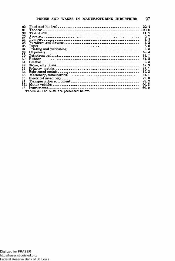
20 Food and kindred...........................— --------- --------------------------------- 22. 421 Tobacco________________________________________________________ 100. 022 Textile mill_____________________________________________________ 11. 923 Apparel________________________________________________________ 5. 724 Lumber------------------------------------------------------------------------------------- 1. 525 Furniture and fixtures___________________________________________ 7. 326 Paper__________________________________________________________ 5. 027 Printing and publishing------------ ------- ------ ------------------------------------ 2. 328 Chemicals______________________________________________________ 59.429 Petroleum refining----- -------------------------- -------------------- ------- --------- 99.130 Rubber_________________________________________________________ 51.231 Leather....... ........... ......... .......................... ............................................... 2. 332 Stone, clay, glass------------------------------------------------------------------------ 57. 933 Primary metals_________________________________________________ 81. 134 Fabricated metals_______________________________________________ 19. 335 Machinery, nonelectrical-------------------------------------------------------------- 31. 136 Electrical machinery____________________________________________ 72. 037 Transportation equipment_______________________________________ 83. 2371 Motor vehicles----------------------------------------------------------------------------- 96. 338 Instruments____________________________________________________ 69.9
Tables A -l to A-21 are presented below.
PRICES AND WAGES IN MANUFACTURING INDUSTRIES 27
Digitized for FRASER http://fraser.stlouisfed.org/ Federal Reserve Bank of St. Louis
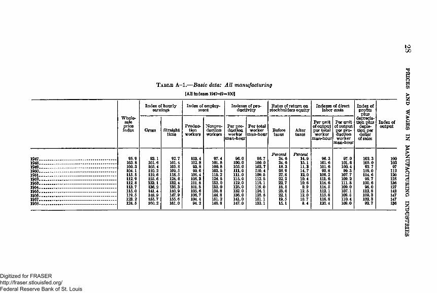
to00
T a b l e A - l . — Basic data: All manufacturing [All indexes 1947-49=100]
Index of hourly earnings
Index of employment
Indexes of productivity
Rates of return on stockholders equity
Indexes of direct labor costs
Index of profits plus
Wholesalepriceindex Gross Straight
timeProduc
tionworkers
Nonproductionworkers
Per production worker
man-hour
Per total worker
man-hourBeforetaxes
Aftertaxes
Per unit of output per total worker
man-hour
Per unit of output per production worker
man-hour
depreciation plus
depletion per dollar
of sales
Index of output
1947............................................................... 95.9 93.1 92.7 103.4 97.4 96.0 96.7Percent
24.6Percent
14.9 96.3 97.0 102.3 1001948............................................................... 103.8 101.6 101.4 102.8 101.8 100.0 100.0 24.6 15.1 101.6 101.6 105.0 1031949............................................................... 100.3 105.4 105.8 93.8 100.8 105.0 103.7 18.3 11.3 101.6 100.4 92.7 971960............................................................... 104.1 110.2 109.5 99.6 103.5 111.0 110.4 26.9 14.7 99.8 99.3 119.0 1121961............................................................... 115.5 119.6 118.5 106.4 115.2 111.0 109.5 27.8 12.0 109.2 107.7 114.6 1201962............................................................... 112.9 125.6 124.6 106.3 124.6 115.0 112.5 22.2 10.4 111.6 109.2 99.7 1251963............................................................... 112.8 133.1 132.4 111.8 133.0 119.0 116.1 22.7 10.6 114.6 111.8 100.6 1361964............................................................... 113.7 136.2 136.3 101.8 133.0 125.0 119.0 18.5 9.9 114.5 109.0 98.0 1271965............................................................... 115.0 141.4 140.9 105.6 136.8 132.0 126.1 23.6 12.5 112.1 107.1 112.8 1421956............................................................... 119.5 148.9 147.9 106.7 144.8 136.0 128.6 22.1 12.0 115.8 109.5 109.3 1471957............................................................... 123.2 155.7 155.6 104.4 151.2 141.0 131.1 19.5 10.7 118.8 110.4 102.3 1471958............................................................... 124.5 160.2 161.0 94.2 148.8 147.0 133.1 15.1 8.4 120.4 109.0 92.7 136
PRICES AND
WAG
ES IN
MA
NU
FAC
TUR
ING
IN
DU
STR
IES
Digitized for FRASER http://fraser.stlouisfed.org/ Federal Reserve Bank of St. Louis
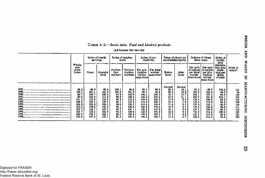
T able A -2 .— Basic data: Food and kindred products[All Indexes 1947-49=100]
Index of hourly earnings
Index of employment
Index of productivity
Rates of return on stockholders equity
Indexes of direct labor costs
Index of profits plus
Wholesalepriceindex Gross Straight
timeProduc
tionworkers
Nonproductionworkers
Per production worker
man-hour
Per total worker
man-hourBeforetaxes
Aftertaxes
Per unit of output per total worker
man-hour
Per unit of output per production worker
man-hour
depreciation plus
depletion per dollar
of sales
Index of output
1947................................................................ 98.2 93.2 92.6 102.1 95.8 97.1 98.8Percent
28.6Percent
16.1 94.3 96.0 112.3 1011948................................................................ 106.1 101.1 101.2 100.3 101.2 99.1 98.8 20.2 12.9 102.3 102.0 93.8 991949................................................................ 95.7 105.7 106.2 97.6 102.9 104.1 102.5 18.7 10.7 103.1 101.5 93.8 1001950................................................................ 99.8 110.6 111.2 96.6 108.4 108.5 105.3 21.0 11.1 105.0 101.9 103.1 1031951................................................................ 111.4 119.0 119.4 96.8 114.6 109.4 104.9 17.8 8.0 113.4 108.8 84.6 1051952................................................................ 108.8 126.5 127.3 96.1 117.2 114.2 108.5 17.4 7.8 116.6 110.8 86.2 1081953................................................................ 104.6 134.0 135.1 96.0 120.3 116.4 109.6 17.8 8.1 122.3 115.1 90.8 1091954................................................................ 105.3 139.0 140.5 93.1 122.8 122.8 113.9 16.8 8.1 122.0 113.2 89.2 1111955................................................................ 101.7 145.7 147.3 92.7 131.1 128.3 116.8 18.1 8.8 124.7 113.6 95.4 1161956................................................................ 101.7 152.3 153.4 93.3 126.8 132.6 121.9 18.9 9.3 124.9 114.9 100.0 1201957................................................................ 105.6 160.7 162.1 90.0 126.6 139.0 126.1 17.2 8.5 127.4 115.6 92.3 1201958................................................................ 110.9 167.3 169.1 87.5 125.8 144.8 130.7 17.4 8.7 128.0 115.5 92.3 122
PRICES AND
WAGES
IN M
ANUFACTURING IN
DUSTRIES
Digitized for FRASER http://fraser.stlouisfed.org/ Federal Reserve Bank of St. Louis
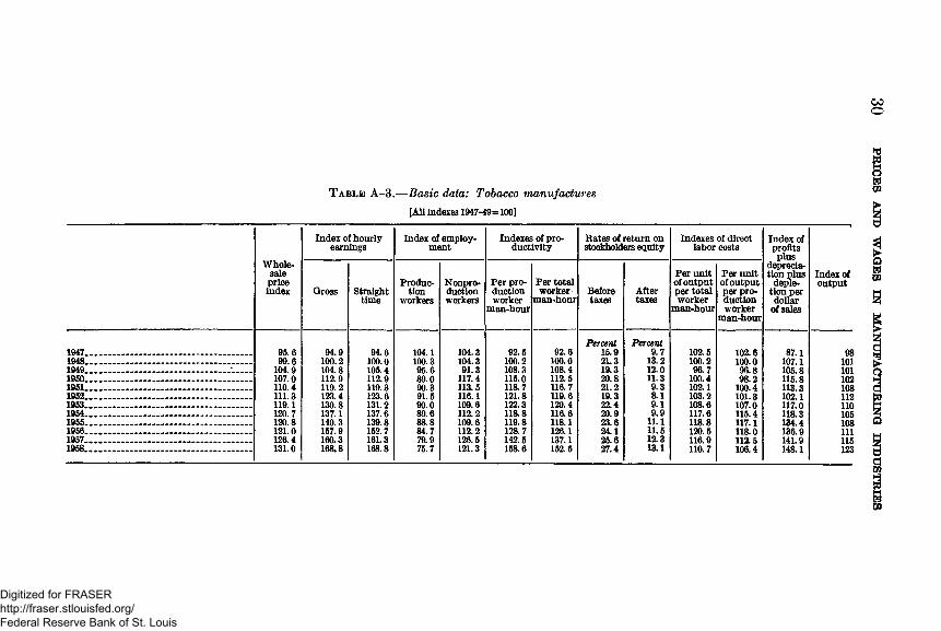
T able A -3 .— Basic data: Tobacco manufactures[All indexes 1947-49=100]
Index of hourly earnings
Index of employment
Indexes of productivity
Rates of return on stockholders equity
Indexes of direct labor costs
Index of profits plus
Wholesalepriceindex Gross Straight
timeProduc
tionworkers
Nonproductionworkers
Per production worker
man-hour
Per total worker
man-hourBeforetaxes
Aftertaxes
Per unit of output per total worker
man-hour
Per unit of output per production worker
man-hour
depreciation plus
depletion per dollar
of sales
Index of output
95.6 94.9 94.6 104.1 104.3 92.5 92.6Percent
15.9Percent
9.7 102.5 102.6 87.1 981948............................................................... 99.6 100.2 100.0 100.3 104.3 100.2 100.0 21.3 13.2 100.2 100.0 107.1 101
104.9 104.8 105.4 95.6 91.3 108.3 108.4 19.3 12.0 96.7 96.8 105.8 101107.0 112.9 112.9 89.0 117.4 115.0 112.5 20.8 11.3 100.4 98.2 115.8 102110.4 119.2 119.3 90.3 113.5 118.7 116.7 21.2 9.3 102.1 100.4 113.3 108111.8 123.4 123.6 91.5 116.1 121.8 119.6 19.3 8.1 103.2 101.3 102.1 112119.1 130.8 131.2 90.0 109.6 122.3 120.4 22.4 9.1 108.6 107.0 117.0 110120.7 137.1 137.6 89.6 112.2 118.8 116.6 20.9 9.9 117.6 115.4 118.3 105120.8 140.3 139.8 88.8 109.6 119.8 118.1 23.6 11.1 118.8 117.1 134.4 108121.0 157.9 152.7 84.7 112.2 128.7 126.1 24.1 11.5 120.5 118.0 136.9 111126.4 160.3 161.3 79.9 126.5 142.5 137.1 25.6 12.3 116.9 112.5 141.9 115
1968................................................................ 131.0 168.8 168.8 75.7 121.3 158.6 152.5 27.4 13.1 110.7 106.4 148.1 123
PRICES AND
WAGES
IN M
ANUFACTURING IN
DUSTRIES
Digitized for FRASER http://fraser.stlouisfed.org/ Federal Reserve Bank of St. Louis

T a b l e A - 4 . — Basic data: Textile mih products[All indexes 1947-49=100]
Index of hourly earnings
Index of employment
Index of productivity
Bates of return on stockholders equity
Indexes of direct labor costs
Index of profits plus
Wholesalepriceindex .Gross Straight
time
Production
workersNonproductionworkers
Per production worker
man-hour
Per total worker
man-hourBeforetaxes
Aftertaxes
Per unit of output per total worker
man-hour
Per unit of output per production worker
man-hour
depreciation plus
depletion per dollar
of sales
Index of output
99.2 92.1 91.9 102.5 95.8 94.9 95.4Percent
33.2Percent
15.9 96.5 97.0 115.8 99105.9 102.8 102.7 104.7 101.5 99.4 99.7 32.6 15.9 103.1 103.4 115.8 10594.9 105.1 105.4 92.8 102.7 106.7 105.7 13.9 6.5 99.4 98.5 68.5 96
101.2 109.3 109.0 98.2 106.1 109.0 108.5 24.0 10.6 100.7 100.3 94.6 109115.9 117.6 117.1 96.1 111.7 110.5 109.2 18.9 6.9 107.7 106.4 77.4 10698.9 120.2 119.8 90.1 109.7 115.9 114.3 9.6 3.6 105.2 103.7 48.1 105
1963............................................................... 95.4 121.1 120.7 89.2 110.3 119.2 117.4 10.0 4.0 103.2 101.6 53.8 10791.8 120.2 120.7 79.9 108.1 127.1 123.9 5.3 1.6 97.0 94.6 39.1 100
1966............................................................... 92.2 122.9 121.6 80.5 107.6 132.5 129.9 11.0 5.0 94.6 92.8 56.3 1)01966................................................................ 91.7 128.2 126.1 79.0 105.8 137.9 135.0 11.6 5.7 95.0 93.0 60.3 1111967................................................................ 91.5 132.6 131.5 74.7 106.0 141.8 137.9 9.1 4.2 96.2 93.5 53.0 1061958............................................................... 88.0 133.5 132.4 69.6 104.6 149.0 144.0 7.9 3.7 92.7 89.6 50.5 103
CO
PBICES AND
WAGES
IN M
ANUPACTUEING IN
DUSTRIES
Digitized for FRASER http://fraser.stlouisfed.org/ Federal Reserve Bank of St. Louis
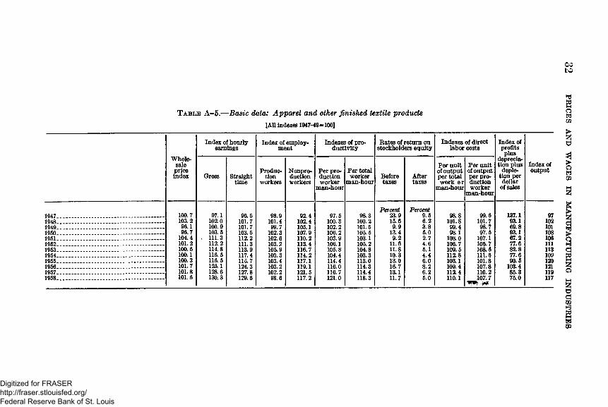
cc to
T a b l e A-5.— Basic data: Apparel and other finished textile products [AU indexes 1947-49=100]
Index of hourly earnings
Index of employment
Indexes of productivity
Rates of return on stockholders equity
Indexes of direct labor costs
Index of profits plus
Wholesalepriceindex Gross Straight
timeProduc
tionworkers
Nonproductionworkers
Per production worker
man-hour
Per total worker
man-hourBeforetaxes
Aftertaxes
Per unit of output per total work er
man-hour
Per unit of output per production worker
man-hour
depreciation plus
depletion per dollar
of sales
Index of output
1947 .............................................................. 100.7 97.1 96.5 98.9 92.4 97.5 98.3Percent
23.9Percent
9.5 98.8 99.6 137.1 971948 ..................... - ...................................... 103.2 102.0 101.7 101.4 102.4 100.3 100.2 15.6 6.2 101.8 101.7 93.1 1021949 ............................................ 96.1 100.9 101.7 99.7 105.1 102.2 101.5 9.9 3.8 99.4 98.7 69.8 1011950 .................................... 96.7 103.5 103.5 102.3 107.9 106.2 105.5 13.4 5.0 98.1 97.5 93.1 1081951 ....................................... 104.4 . 111.3 112.2 102.6 110.2 103.9 103.1 9.2 2.7 108.0 107.1 67.2 1061952 ............................— 101.2 112.2 111.3 103.2 113.4 106.1 105.2 11.6 4.6 106.7 105.7 77.6 1111953 ....... ......................... 100.6 114.8 113.9 105.9 116.7 105.8 104.8 11.8 5.1 109.5 108.5 82.8 1131954 ............................... 100.1 116.5 117.4 100.3 114.2 104.4 103.3 10.3 4.4 112.8 111.6 77.6 1091955 ............................. 100.3 116.5 115.7 103.4 117.1 114.4 113.0 13.0 6.0 103.1 101.8 90.5 1201956 ............................. 101.7 125.1 124.3 103.2 119.1 116.0 114.3 16.7 8.2 109.4 107.8 103.4 1211957 ............................. 101.8 128.6 127.8 102.2 121.5 116.7 114.4 13.1 6.2 112.4 110.2 85.3 1191958 ............................ 101.6 130.3 129.6 98.6 117.2 121.0 118.3 11.7 5.0 110.1 107.7 75.0 117
PRICES AND
WAGES
IN M
ANUFACTURING IN
DUSTRIES
Digitized for FRASER http://fraser.stlouisfed.org/ Federal Reserve Bank of St. Louis
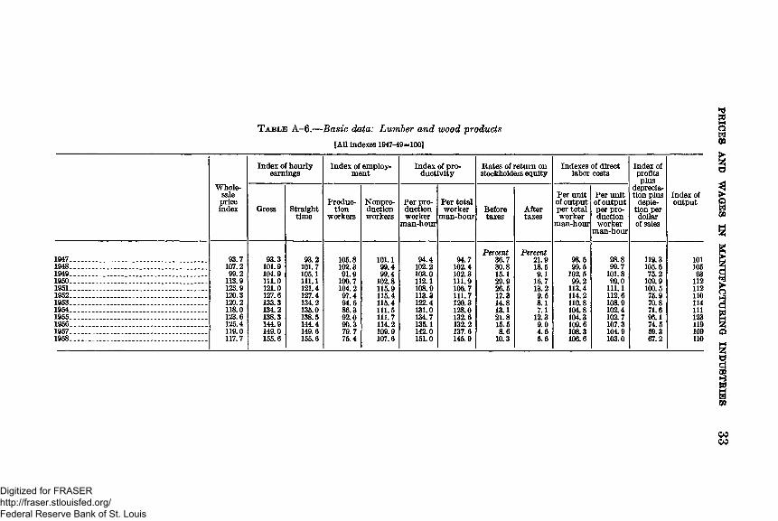
T able A -6 .— Basic data: Lumber and wood products
[All indexes 1947-49=100]
Index of hourly earnings
Index of employment
Index of productivity
Bates of return on stockholders equity
Indexes of direct labor costs
Index of profits plus
Wholesalepriceindex Gross Straight
timeProduc
tionworkers
Nonproductionworkers
Per production worker
man-hour
Per total worker
man-hourBeforetaxes
Aftertaxes
Per unit of output per total worker
man-hour
Per unit of output per production worker
man-hour
depreciation plus
depletion per dollar
of sales
Index of output
1947.......................... .................................... 93.7 93.3 93.2 105.8 101.1 94.4 94.7Percent
36.7Percent
21.9 98.5 98.8 119.3 1011948............................................................... 107.2 101.9 101.7 102.3 99.4 102.2 102.4 30.8 18.5 99.5 99.7 105.5 1051949............................................................... 99.2 104.9 105.1 91.9 99.4 103.0 102.3 15.1 9.1 302.5 101.8 75.2 931950..................... ....................................... 113.9 111.0 111.1 100.7 102.8 112.1 111.9 29.9 16.7 99.2 99.0 109.9 1121951............................................................. 123.9 121.0 121.4 104.2 115.9 108.9 106.7 26.5 13.2 113.4 111.1 100.5 1121952............................................................... 120.3 127.6 127.4 97.4 115.4 113.3 111.7 17.3 9.5 114.2 112.6 75.9 1101953................................. ............................. 120.2 133.3 134.2 94.6 115.4 122.4 120.3 14.8 8.1 110.8 108.9 70.8 1141954............................................................... 118.0 134.2 135.0 86.3 111.5 131.0 128.0 13.1 7.1 104.8 102.4 71.6 1111955............................................................... 123.6 138.3 138.5 92.0 111.7 134.7 132.6 21.8 12.3 104.3 102.7 96.1 1231956.............................................. ............... 125.4 144.9 144.4 90.3 114.2 135.1 132.2 15.5 9.0 109.6 107.3 74.5 1191957............................................................... 119.0 149.0 149.6 79.7 109.9 142.0 137.6 8.6 4.6 108.3 104.9 59.3 1091958............................................................... 117.7 155.6 155.6 75.4 107.6 151.0 145.9 10.3 5.6 106.6 103.0 67.2 110
PRICES AND
WAGES
IN M
ANUFACTURING INDtTSTBIES
Digitized for FRASER http://fraser.stlouisfed.org/ Federal Reserve Bank of St. Louis
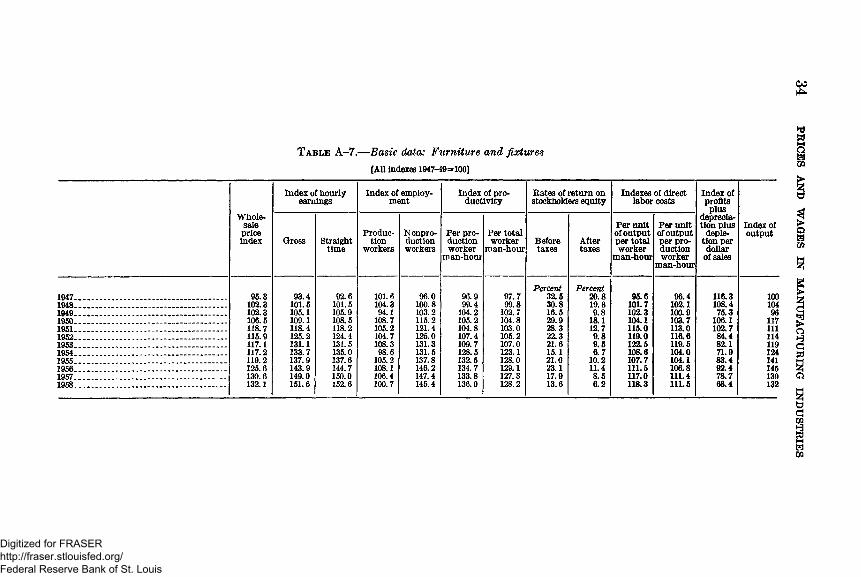
T able A -7 .— Basic data: Furniture and fixtures
[All indexes 1947-49=100]
Index of hourly earnings
Index of employment
Index of productivity
Rates of return on stockholders equity
Indexes of direct labor costs
Index of profits plus
Wholesalepriceindex Gross Straight
timeProduc
tionworkers
Nonproductionworkers
Per production worker
man-hour
Per total worker
man-hourBeforetaxes
Aftertaxes
Per unit of output per total worker
man-hour
Per unit of output per production worker
man-hour
depreciation plus
depletion per dollar
of sales
Index of output
1947................................................................ 95.3 93.4 92.6 101.6 96.0 96.9 97.7Percent
32.5Percent
20.8 95.6 96.4 116.3 1001948................................................................ 102.3 101.5 101.5 104.3 100.8 99.4 99.8 30.8 19.8 101.7 102.1 108.4 1041949............................................................... 102.3 105.1 105.9 94.1 103.2 104.2 102.7 16.5 9.8 102.3 100.9 75.3 961960................................................................ 106.5 109.1 108.5 108.7 115.2 105.2 104.8 29.9 18.1 104.1 103.7 106.1 1171961....................................................- .......... 118.7 118.4 118.2 105.2 121.4 104.8 103.0 28.3 12.7 115.0 113.0 102.7 1111962.............................................................. - 115.9 125.2 124.4 104.7 125.0 107.4 105.2 22.3 9.8 119.0 116.6 84.4 1141953................................................................ 117.1 131.1 131.5 108.3 131.3 109.7 107.0 21.6 9.5 122.5 119.5 82.1 1191954............................................................... 117.2 133.7 135.0 98.6 131.5 128.5 123.1 15.1 6.7 108.6 104.0 71.9 1241955....................... ........................................ 119.2 137.9 137.6 105.2 137.8 132.5 128.0 21.0 10.2 107.7 104.1 83.4 1411956............................................................... 125.6 143.9 144.7 108.1 146.2 134.7 129.1 23.1 11.4 111.5 106.8 92.4 1451957............................................................... 130.6 149.0 150.0 106.4 147.4 133.8 127.3 17.9 8.5 117.0 111.4 78.7 1391958............................................................... 132.1 151.6 152.6 100.7 145.4 136.0 128.2 13.6 6.2 118.3 111.6 68.4 132
PRICES AND
WAGES
IN M
ANUFACTURING IN
DUSTRIES
Digitized for FRASER http://fraser.stlouisfed.org/ Federal Reserve Bank of St. Louis

T able A -8 .— Basic data: Paper and allied products
[All indexes 1947-49=100]
Index of hourly earnings
Index of employment
Index of productivity
Rates of return on stockholders equity
Indexes of direct labor costs
Index of profits plus
Wholesalepriceindex Gross Straight
timeProduc
tionworkers
Nonproductionworkers
Per production worker
man-hour
Per total worker
man-hourBeforetaxes
Aftertaxes
Per unit of output per total worker
man-hour
Per unit of output per production worker
depreciation plus
depletion per dollar
of sales
Index of output
1047..........................................- .................... 98.6 92.0 91.2 101.3 92.7 97.4 98.7Percent
33.1Percent
20.5 93.2 94.5 119.1 1001948............................................................... 102.9 102.0 101.9 101.6 103.7 99.8 99.6 25.9 16.0 102.4 102.2 98.1 1021949................................................................ 98.5 106.0 106.9 97.1 103.7 103.0 101.8 16.6 10.3 104.1 102.9 82.8 981950............................................................... 100.9 111.5 110.2 103.6 109.9 111.9 111.3 26.8 15.3 100.2 99.6 110.2 1181951............................................................... 119.6 120.1 119.3 108.3 121.1 113.9 112.4 35.0 13.9 106.9 105.4 122.3 125
116.5 127.2 126.8 105.0 130.0 112.6 109.3 23.6 10.4 116.4 113.0 102.5 1191953............................................................... 116.1 133.5 132.6 110.3 139.2 116.6 113.0 22.3 10.1 118.1 114.5 96.2 1301954............................................................... 116.3 138.2 138.4 109.8 143.7 120.9 116.2 19.8 9.9 118.9 114.3 94.3 1321955............................................................... 119.3 144.5 143.4 112.9 153.1 130.5 125.0 22.6 11.5 115.6 110.7 99.4 1491956............................................................... 127.2 153.2 152.5 115.7 163.8 134.1 127.3 22.2 11.4 120.3 114.2 98.1 1561957............................................................... 129.6 161.1 160.8 114.5 168.9 136.1 128.1 17.6 9.0 125.8 118.4 85.3 1551958............................................................... 131.0 167.5 167.4 109.6 169.3 145.4 135.4 14.8 7.6 123.7 115.2 80.9 157
PRICES AND
WAGES
IN M
ANU
FACTUR
ING
IN
DU
STR
IES
Digitized for FRASER http://fraser.stlouisfed.org/ Federal Reserve Bank of St. Louis
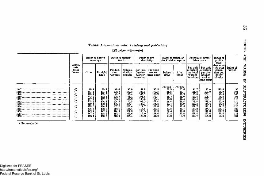
T able A -9 .— Basic data: Printing and publishing[All indexes 1947-49=100]
Index of hourly earnings
Index of employment
Index of productivity
Rates of return on stockholders equity
Indexes of direct labor costs
Index of profits plus
Wholesalepriceindex Gross Straight
timeProduc
tionworkers
Nonproductionworkers
Per production worker
man-hour
Per total worker
man-hourBeforetaxes
Aftertaxes
Per unit of output per total worker
man-hour
Per unit of output per production worker
man-hour
depreciation plus
depletion per dollar
of sales
Index of output
1947........... ................................................... 0) 90.4 89.8 99.4 96.0 94.8 96.5Percent
28.9Percent
20.6 93.7 95.4 110.6 961948............................................................... 0) 101.3 101.2 100.9 100.5 100.3 100.3 24.6 17.1 101.0 101.0 98.9 1011949............................................................... 0) 108.4 109.0 99.7 103.4 105.1 103.2 20.2 13.9 105.0 103.1 90.4 1031950........... ................................................... 0) 112.2 112.6 100.9 108.4 108.6 105.4 21.5 14.0 106.5 103.3 96.8 108
(1) 117.1 117.5 103.1 107.9 108.3 106.1 24.0 12.5 110.4 108.1 108.5 1101952........— .................................................. 0) 123.6 124.1 104.8 110.8 107.2 104.4 21.6 11.4 118.4 115.3 97.9 no
(') 129.4 130.1 106.6 115.1 109.1 105.8 22.1 11.9 122.3 118.6 98.9 1151954......... ..................................................... 0) 133.6 134.3 107.2 118.4 114.7 109.8 20.2 11.5 121.7 116.5 94.7 120
0) 138.3 138.6 110.1 121.4 116.8 112.3 22.8 12.7 123.2 118.4 101.1 1270)0)
142.4 142.8 114.3 124.0 118.9 115.0 24.5 13.0 123.8 119.8 103.2 1341957................ ............................................. - 147.1 148.2 115.1 125.6 119.0 114.6 22.2 11.4 128.4 123.6 96.8 1341958................ ............................................. - 0) 152.4 153.6 113.4 126.4 120.2 114.0 18.0 8.9 133.7 126.8 88.3 131
i Not available.
PRICES AND
WAGES
IN M
ANtTPACTU
RIN
G
IND
USTR
IES
Digitized for FRASER http://fraser.stlouisfed.org/ Federal Reserve Bank of St. Louis
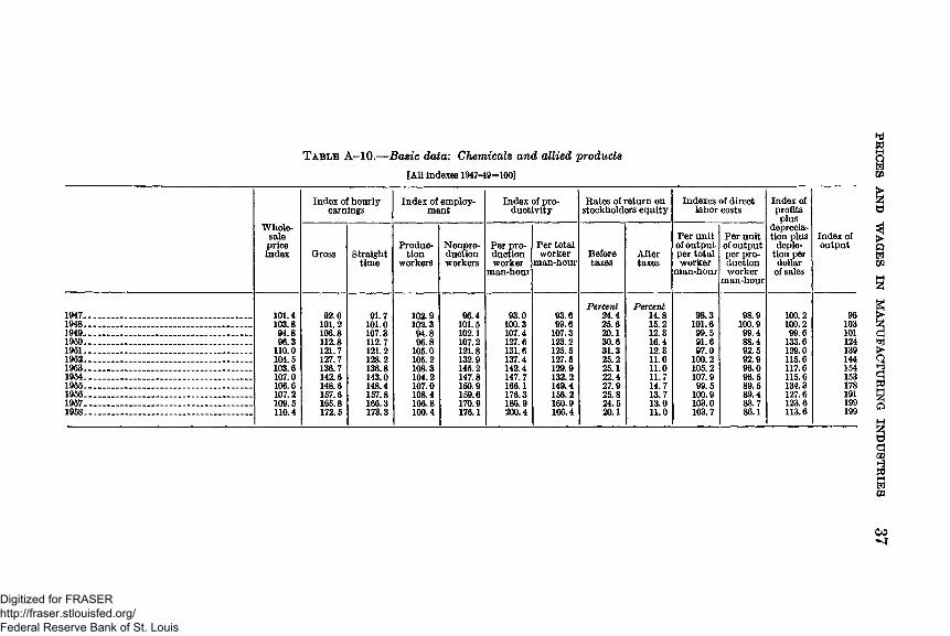
T able A -1 0 .— Basic data: Chemicals and allied products
[All indexes 1947-49=100]
Index of hourly earnings
Index of employment
Index of productivity
Rates of return on stockholders equity
Indexes of direct labor costs
Index of profits plus
Wholesalepriceindex Gross Straight
timeProduc
tionworkers
Nonproductionworkers
Per production worker
man-hour
Per total worker
man-hourBeforetaxes
Aftertaxes
Per unit of output per total worker
man-hour
Per unit of output per production worker
man-hour
depreciation plus
depletion per dollar
of sales
Index of output
1947............................................................... 101.4 92.0 91.7 102.9 96.4 93.0 93.6Percent
24.4Percent
14.8 98.3 98.9 100.2 961948............................................................... 103.8 101.2 101.0 102.3 101.5 100.3 99.6 25.6 15.2 101.6 100.9 100.2 1031949................................................................ 94.8 106.8 107.3 94.8 102.1 107.4 107.3 20.1 12.3 99.5 99.4 99.6 1011950................................................................ 96.3 112.8 112.7 96.8 107.2 127.6 123.2 30.6 16.4 91.6 88.4 133.6 1241951............................................................... 110.0 121.7 121.2 105.0 121.8 131.6 125.5 31.3 12.3 97.0 92.5 129.0 1391952............................................................... 104.5 127.7 128.2 105.2 132.9 137.4 127.5 25.2 11.0 100.2 92.9 115.6 1441953................................................................ 103.6 136.7 136.8 108.3 145.2 142.4 129.9 25.1 11.0 105.2 96.0 117.6 1541954............................................................... 107.0 142.6 143.0 104.2 147.8 147.7 132.2 22.4 11.7 107.9 96.5 115.6 1531955............................................................... 106.6 148.6 148.4 107.0 150.9 166.1 149.4 27.9 14.7 99.5 89.5 134.3 1781956............................................................... 107.2 157.6 157.8 108.4 159.6 176.3 156.2 25.8 13.7 100.9 89.4 127.6 1911957............................................................... 109.5 165.8 166.3 106.8 170.9 186.9 160.9 24.5 13.0 103.0 88.7 123.6 1991958................................................................ 110.4 172.5 173.3 100.4 176.1 200.4 166.4 20.1 11.0 103.7 86.1 113.6 199
00<1
PRICES AND
WAG
ES IN
MA
NU
FAC
TUR
ING
IN
DU
STR
IES
Digitized for FRASER http://fraser.stlouisfed.org/ Federal Reserve Bank of St. Louis
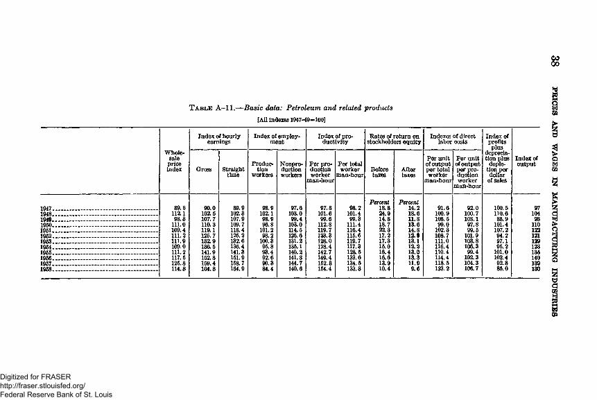
T a b le A - l l .— Basic data: Petroleum and related products[All Indexes 1947-49=100]
Index of hourly earnings
Index of employment
Index of productivity
Rates of return on stockholders equity
Indexes of direct labor costs
Index of profits plus
Wholesalepriceindex Gross Straight
timeProduc
tionworkers
Nonproductionworkers
Per production worker
man-hour
Per total worker
man-hourBeforetaxes
Aftertaxes
Per unit of output per total worker
man-hour
Per unit of output per production worker
man-hour
depreciation plus
depletion per dollar
of sales
Index of output
1947............................................................... 89.6 90.0 89.9 98.9 97.6 97.8 98.2Percent
18.8Percent
14.2 91.6 92.0 100.5 971948............................................................... 112.1 102.5 102.3 102.1 103.0 101.6 101.4 24.9 18.6 100.9 100.7 110.6 1041949............................................................... 98.3 107.7 107.9 98.9 99.4 99.6 99.3 14.8 11.8 108.5 108.1 88.9 981950............................................................... 111.0 110.3 109.7 96.8 103.0 112.8 111.4 18.7 13.6 99.0 97.8 101.4 1101951........................................- ____________ 109.4 119.1 118.4 101.2 114.5 119.7 116.4 22.3 14.8 102.3 99.5 107.2 1221952............................................................... 111.2 125.7 125.2 98.2 126.6 123.3 115.6 17.2 12.9 108.7 101.9 94.2 1211953............................................................... 111.9 132.9 132.6 100.3 131.2 128.0 119.7 17.3 13.1 111.0 103.8 97.1 1291954............................................................... 109.0 136.5 136.4 95.3 135.1 128.4 117.3 15.0 12.2 116.4 106.3 95.2 1231955............................................................... 111.2 141.9 141.3 93.4 140.2 142.7 128.5 16.4 13.0 110.4 99.4 101.0 1351956............................................................... 117.5 152.8 151.9 92.6 141.8 149.4 133.6 16.6 13.3 114.4 102.3 102.4 1401957............................................................... 125.8 159.4 158.7 90.3 144.7 152.8 134.5 13.9 11.9 118.5 104.3 92.8 1391958............................................................... 114.8 164.8 164.9 84.4 140.6 154.4 133.8 10.4 9.6 123.2 106.7 85.0 130
PBICBS AND
WAGES
IN M
ANUFACTURING IN
DUSTRIES
Digitized for FRASER http://fraser.stlouisfed.org/ Federal Reserve Bank of St. Louis
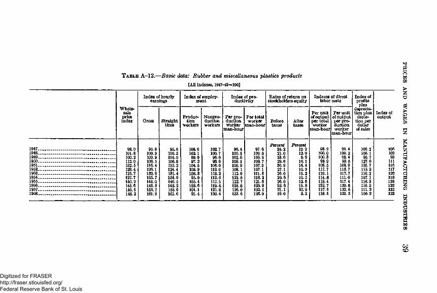
T a b le A -1 2 .— Basic data: Rubber and miscellaneous plastics products
[AH indexes, 1947-49=100]
Index of hourly earnings
Index of employment
Index of productivity
Bates of return on stockholders equity
Indexes of direct labor costs
Index of profits plus
Wholesalepriceindex Gross Straight
timeProduc
tionworkers
Nonproductionworkers
Per production worker
man-hour
Per total worker
man-hourBeforetaxes
Aftertaxes
Per unit of output per total worker
man-hour
Per unit of output per production worker
man-hour
depreciation plus
depletion per dollar
of sales
Index of output
1947............................................................... 98.0 95.8 95.6 108.0 102.7 96.4 97.6Percent
24.2Percent
12.2 98.2 99.4 109.2 1061948............................................................... 101.8 100.3 100.5 102.1 100.7 100.1 100.3 21.0 12.0 100.0 100.2 105.1 1021949............................................................... 100.2 103.9 104.0 89.9 96.6 105.6 103.6 13.6 8.6 100.3 98.4 85.7 931950............................................................... 112.0 108.5 106.8 97.2 98.6 109.1 109.7 29.6 16.1 98.9 99.5 127.6 1111951............................................................... 132.5 116.4 115.2 104.5 106.0 106.9 107.3 36.9 14.4 108.5 108.9 135.7 1161952................................................................ 128.4 126.1 124.4 103.9 113.0 108.1 107.1 27.1 10.9 117.7 116.7 113.3 1171953............................................................... 125.7 132.9 131.4 108.3 118.2 112.9 111.6 26.0 11.2 119.1 117.7 110.2 1261954............................................................... 127.7 135.7 134.9 95.0 113.6 122.3 118.2 20.6 10.5 114.8 111.0 107.1 1181955............................................................... 140.2 144.0 140.5 105.4 117.5 122.7 121.6 26.0 12.6 118.4 117.4 116.3 1381956................................................................ 145.6 149.5 148.2 103.6 119.4 123.8 120.9 23.6 11.8 123.7 120.8 116.3 1321957................................................................ 146.5 u u 153.9 101.1 121.8 126.0 122.1 21.1 10.9 127.5 123.6 111.2 1321958___________________________________ 148.2 161.9 161.6 91.4 120.4 133.6 126.0 19.0 9.3 128.5 121.2 109.2 123
CCo
PRICES AND
WAGES
IN M
ANUFACTURING IN
DUSTRIES
Digitized for FRASER http://fraser.stlouisfed.org/ Federal Reserve Bank of St. Louis
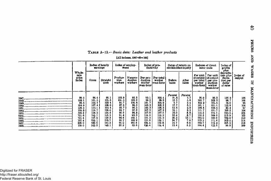
T a b le A -13 .— Basic data: Leather and leather products[All indexes, 1947-49=100]
Index of hourly earnings
Index of employment
Index of productivity
Rates of return on stockholders equity
Indexes of direct labor costs
Index of profits plus
depreciation plus
depletion per dollar
of sales
Wholesalepriceindex Gross Straight
timeProduc
tionworkers
Nonproductionworkers
Per production worker
man-hour
Per total worker
man-hourBeforetaxes
Aftertaxes
Per unit of output per total worker
man-hour
Per unit of output per production worker
man-hour
Index of output
99.5 95.4 95.1 102.9 93.3 99.1 100.4Percent
21.8Percent
7.7 95.0 96.3 127.2 105102.1 101.5 101.5 101.5 105.9 99.3 98.8 15.9 5.8 102.7 102.2 98.7 10098.4 103.1 103.4 95.7 100.8 101.7 100.9 9.7 3.4 102.2 101.4 74.0 95
104.9 107.4 108.0 97.6 98.3 106.2 106.2 17.7 6.1 101.1 101.1 113.9 104120.5 115.1 115.4 93.7 96.3 105.2 108.2 12.6 2.9 106.4 109.4 854 97103.8 119.7 120.0 94.7 97.6 107.2 107.2 15.1 8.2 111.7 111.7 106.3 104104.3 124.2 124.6 95.9 99.3 107.9 107.5 16.0 8.8 115.5 115.1 110.1 104101.6 125.1 125.5 91.4 99.3 114.5 113.2 15.4 8.7 110.5 109.3 113.9 103101.4 127.8 128 3 94.6 103.1 117.2 116.2 20.2 12.1 110.0 109.0 132.9 112
1956 ....................................... ................ 107.4 135.1 135.7 93.7 102.9 121.3 120.1 14.7 7.0 112.5 111.4 102.5 1141957 — .................................. - ........ ...... 108.0 139.6 140.3 91.0 102.6 124.4 122.8 14.7 6.9 113.7 112.2 104.4 1131958 ................... ...................................... 109.0 142.3 143.1 87.9 99.6 126.4 124.4 12.4 5.5 114.4 112.6 94.9 109
PRICES AND
WAGES
IN M
ANUFACTUKING IN
DUSTRIES
Digitized for FRASER http://fraser.stlouisfed.org/ Federal Reserve Bank of St. Louis
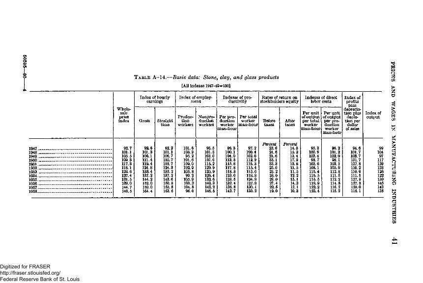
50505—60- T a b l e A -1 4 .— Basic data: Stone, clay, and glass products
[All indexes 1947-49=100]
Index of hourly earnings
Index of employment
Indexes of productivity
Rates of return on stockholders equity
Indexes of direct labor costs
Index of profits plus
Wholesalepriceindex Gross Straight
timeProduc
tionworkers
Nonproductionworkers
Per production worker
man-hour
Per total worker
man-hourBeforetaxes
Aftertaxes
Per unit of output per total worker
man-hour
Per unit of output per production worker
man-hour
depreciation plus
depletion per dollar
of sales
Index of output
1947............................................................... 92.7 92.6 92.2 101.6 95.5 96.3 97.2Percent
23.6Percent
14.3 95.3 96.2 94.6 991948............................................................... 101.1 103.3 101.1 103.2 101.5 100.1 100.4 24.6 15.2 100.9 101.2 101.7 1041949 ............................................................. 105.5 106.1 106.7 95.2 103.0 104.0 102.6 21.6 13.4 103.4 102.0 103.7 971950 ............................................................. 109.3 111.4 110.7 101.6 107.6 113.5 112.9 33.1 17.9 98.7 98.1 131.7 1171951 - ............................................................ 117.3 119.4 118.7 109.0 115.2 115.8 115.3 33.3 13.8 103.6 103.1 127.8 1291952 .............................................................. 118.1 124.8 124.3 102.9 120.9 117.8 115.4 25.0 11.5 108.1 105.9 110.2 1231953 ............ ............ .................................. 123.6 133.4 133.2 105.8 125.9 118.3 115.6 25.2 11.5 115.4 112.8 110.9 1261954 .............................................................. 127.4 137.2 137.2 99.2 126.4 123.0 118.8 23.0 12.2 115.5 111.5 111.5 1221955........................................- ..................... 131.5 144.2 143.6 105.9 132.6 128.5 124.8 29.0 15.1 115.5 112.2 127.8 1391956 ............................................................ 139.0 152.0 150.8 108.2 140.3 132.4 127.8 27.4 14.3 118.9 114.8 127.8 1451957............................................................... 144.7 159.0 158.8 104.8 142.2 136.8 130.1 22.5 12.1 122.2 116.2 120.0 1431958............................................................... 149.5 164.4 163.6 96.0 146.5 142.7 133.2 19.0 10.3 123.4 115.2 116.1 135
PRICES AND
WAGES
IN M
ANUFACTURING IN
DU
STRIES
Digitized for FRASER http://fraser.stlouisfed.org/ Federal Reserve Bank of St. Louis
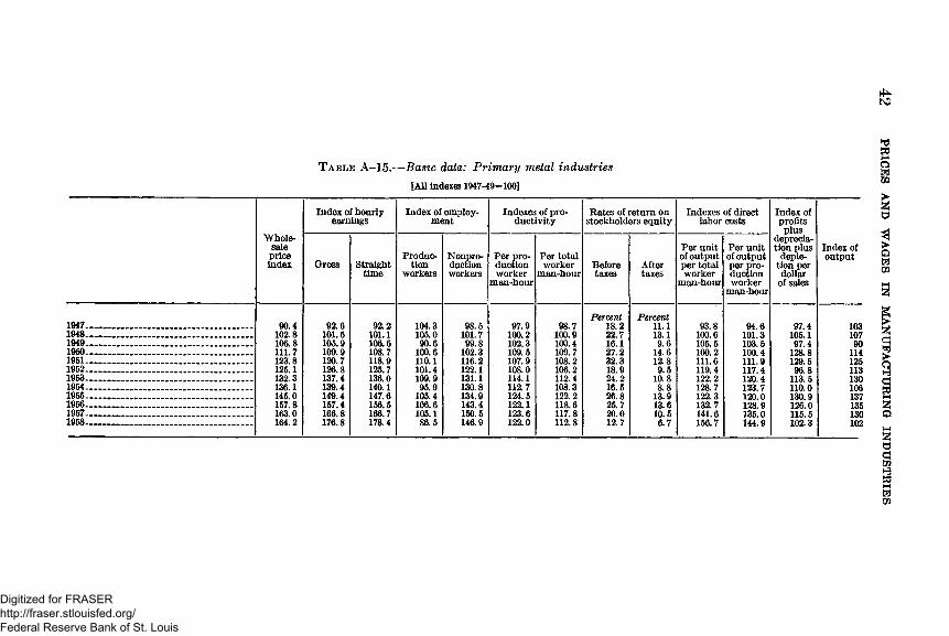
T a b le A - l 5.— Basic data: Primary metal industries[All indexes 1947-49=100]
Index of hourly earnings
Index of employment
Indexes of productivity
Rates of return on stockholders equity
Indexes of direct labor costs
Index of profits plus
depreciation plus
depletion per dollar
of sales
Wholesalepriceindex Gross Straight
timeProduc
tionworkers
Nonproductionworkers
Per production worker
man-hour
Per total worker
man-hourBeforetaxes
Aftertaxes
Per unit of output per total worker
man-hour
Per unit of output per production worker
man-hour
Index of output
1947............................................................... 90.4 92.6 92.2 104.3 98.5 97.9 98.7Percent
18.2Percent
11.1 93.8 94.6 97.4 1031948............................................................... 102.8 101.5 101.1 105.0 101.7 100.2 100.9 22.7 13.1 100.6 101.3 105.1 1071949............................................................... 106.8 105.9 106.6 90.6 99.8 102.3 100.4 16.1 9.6 105.5 103.5 97.4 90
111.7 109.9 108.7 100.6 102.3 109.5 109.7 27.2 14.6 100.2 100.4 128.8 114123.8 120.7 118.9 110.1 116.2 107.9 108.2 32.3 12.8 111.6 111.9 129.5 125
1952............................................................... 125.1 126.8 125.7 101.4 122.1 108.0 106.2 18.9 9.5 119.4 117.4 96.8 1131953............................................................... 132.3 137.4 136.0 109.9 131.1 114.1 112.4 24.2 10.8 122.2 120.4 113.5 130
136.1 139.4 140.1 95.9 130.8 112.7 108.3 16.5 8.8 128.7 123.7 110.0 1061955............................................................... 145.0 149.4 147.6 105.4 134.9 124.5 122.2 26.8 13.9 122.3 120.0 130.9 1371956............................................................... 157.8 157.4 156.5 106.6 143.4 122.1 118.6 25.7 13.6 132.7 128.9 126.0 1351957............................................................... 163.0 166.8 166.7 105.1 150.5 123.6 117.8 20.0 10.5 141.6 135.0 115.5 130
164.2 176.8 178.4 86.5 146.9 122.0 112.8 12.7 6.7 156.7 144.9 102.3 102
PRICES AND
WAGES
IN M
ANUFACTURING IN
DU
STRIES
Digitized for FRASER http://fraser.stlouisfed.org/ Federal Reserve Bank of St. Louis
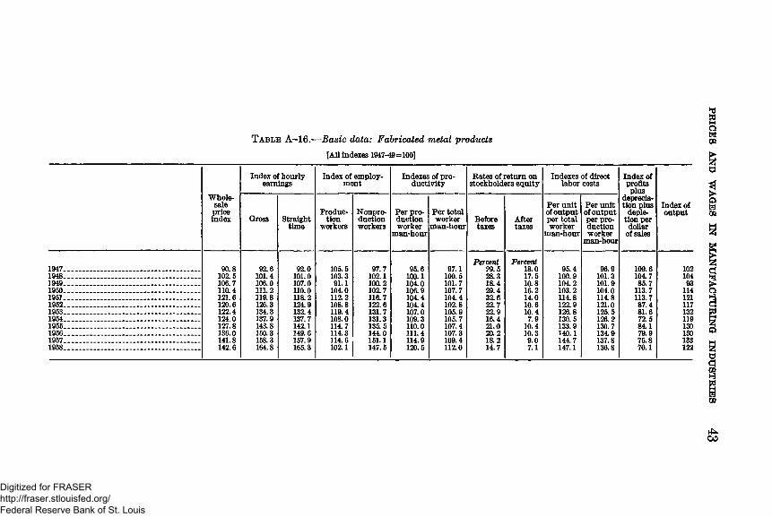
T able A -16 .— Basic data: Fabricated metal products
[All indexes 1947-49=100]
Index of hourly earnings
Index of employment
Indexes of productivity
Rates of return on stockholders equity
Indexes of direct labor costs
Index of profits plus
Wholesalepriceindex Gross Straight
time
Production
workersNonproductionworkers
Per production worker
man-hour
Per total worker
man-hourBeforetaxes
Aftertaxes
Per unit of output per total worker
man-hour
Per unit of output per production worker
man-hour
depreciation plus
depletion per dollar
of sales
Index of output
1947............................................................... 90.8 92.6 92.0 105.5 97.7 95.6 97.1Percent
29.5Percent
18.0 95.4 96.9 109.6 1021948............................................................... 102.5 101.4 101.0 103.3 102.1 100.1 100.5 28.3 17.5 100.9 101.3 104.7 1041949............................................................... 106.7 106.0 107.0 91.1 100.2 104.0 101.7 18.4 10.8 104.2 101.9 85.7 931950............................................................... 110.4 111.2 110.0 104.0 102.7 106.9 107.7 29.4 16.2 103.2 104.0 113.7 114195]............................................................... 121.6 119.8 118.2 112.2 116.7 104.4
104.4104.4 32.6 14.0 114.8 114.8 113.7 121
1952............................................................... 120.6 126.3 124.9 108.8 122.6 102.8 22.7 10.610.47.9
122.9 121.0 87.4 1171953............................................................... 122.4 134.3 132.4 119.4 131.7 107.0 105.9 22.9 126.8 125.5 81.6 1321954............................................................... 124.0 137.9 137.7 108.0 131.3 109.3 105.7 16.4 130.5 126.2 72.5 1191955............................................................... 127.8 143.8 142.1 114.7 135.5 110.0 107.4 21.0 10.4 133.9 130.7 84.1 1301956............................................................... 336.0 150.3 149.6 114.3 144.0 111.4 107.3 20.2 10.3 140.1 134.9 79.9 1301957............................................................... 141.8 158.3 157.9 114.6 |, 151.1 114.9 109.4 18.2 9.0 144.7 137.8 75.8 1331958............................................................... 142.6 164.8 165.3 102.1 1 147.5 120.5 112.0 14.7 7.1 147.1 136.8 70.1 122
CO
PRICES AND
WAGES
IN M
ANUFACTURING IN
DUSTRIES
Digitized for FRASER http://fraser.stlouisfed.org/ Federal Reserve Bank of St. Louis
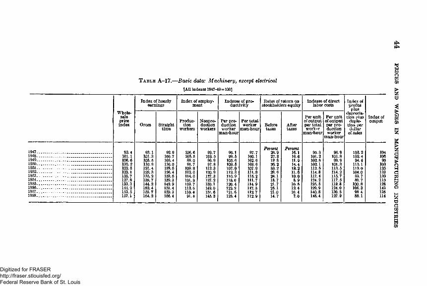
T a b l e A-17.— Basic data: Machinery, except electrical[All indexes 1947-49=100]
Index of hourly earnings
Index of employment
Indexes of productivity
Rates of return on stockholders equity
Indexes of direct labor costs
Index of profits plus
depreciation plus
depletion per dollar
of sales
Wholesalepriceindex Gross Straight
timeProduc
tionworkers
Nonproductionworkers
Per production worker
man-hour
Per total worker
man-hourBeforetaxes
Aftertaxes
Per unit of output per total worker
man-hour
Per unit of output per production worker
man-hour
Index of output
1947............................................................... 92.4 93.1 92.9 106.6 99.7 96.1 97.7Percent
26.9Percent
16.1 95.3 96.9 103.2 1041948-............................................................. 101.1 101.3 100.7 105.5 103.5 99.5 100.1 27.3 16.6 101.2 101.8 102.4 1061949............................................................... 106.6 105.5 106.4 88.0 96.9 105.6 102.6 19 8 11.9 102.8 99.9 94.4 901950................ .............................................. 110.2 110.9 110.0 91.7 97.8 109.5 108.6 26.2 14.4 102.1 101.3 115.1 1031951............................... ............................... 122.5 121.4 118.6 109.8 112.3 107.0 107.9 33.2 13.2 112.5 113.5 119.0 1251952................................... .......................... 123.1 128.3 126.4 112.6 120.9 112.3 111.8 28.6 11.6 114.8 114.2 104.0 1331953................................. ........................... 125.7 335.2 133.6 114.6 127.3 116.9 115.2 24.1 10.0 117.4 115.7 93.7 1391954................ ................... ......................... 127.8 138.7 139.3 101.3 127.2 118.0 111.7 18.7 8.9 124.2 117.5 89.7 1191955................ ................... .......................... 133.3 144.2 142.9 103.7 130.1 120.4 114.9 21.7 10.5 125.5 119.8 100.8 1281956........................................................ . . 144.2 152.4 151.4 112.5 142.0 122.9 117.3 25.1 12.4 129.9 124.0 106.3 1431957.............. ............................................... 153. 5 158.7 159.3 110.4 151.6 121.6 112.7 21.0 10.4 140.8 130.5 98 4 1351958_____ _____ _________________ ______ 157.1 164.2 166.4 91.4 145.3 128.4 112.9 14.7 7.0 145.4 127.9 88.1 114
PRICES AND
WAGES
IN M
ANUFACTURING IN
DUSTRIES
Digitized for FRASER http://fraser.stlouisfed.org/ Federal Reserve Bank of St. Louis
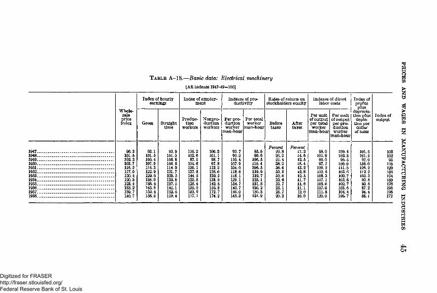
T a b l e A - 18.— Basic data: Electrical machinery
[All indexes 1947-49=100]
Index of hourly earnings
Index of employment
Indexes of productivity
Rates of return on stockholders equity
Indexes of direct labor costs
Index of profits plus
depreciation plus
depletion per dollar
of sales
Wholesalepriceindex Gross Straight
time
Production
workersNonproductionworkers
Per production worker
man-hour
Per total worker
man-hourBeforetaxes
Aftertaxes
Per unit of output per total worker
man-hour
Per unit of output per production worker
man-hour
Index of output
1947............................................................... 96.3 93.1 92.9 110.2 100.2 92.7 95.0Percent
29.8Percent
17.2 98.0 100.4 101.5 1031948............................................................... 101.5 101.5 101.3 102.6 101.1 99.2 99.6 26.2 14.6 101.9 102.3 101.5 1021949.— ........................................................ 102.2 105.4 105.8 87.1 98.7 110.4 106.5 21.4 12.5 99.0 95.5 97.0 951960............................................................... 103.7 107.9 106.5 104.6 97.8 107.9 110.4 38.2 18.4 97.7 100.0 138.0 1161961............................................................... 116.2 116.3 114.9 120.1 112.2 104.0 106.5 36.6 13.2 109.2 111.8 128.2 1291952..................... ......................................... 117.0 122.9 121.7 127.6 126.0 118.6 119.9 33.5 12.8 102.5 103.6 112.2 1561953............................................................... 120.4 129.6 128.5 144.5 139.2 118.1 119.7 32.0 12.5 108.3 109.7 103.3 1741954............................................................... 120.3 134.0 133.8 123.8 138.9 129.1 125.1 23.6 11.7 107.1 103.8 93.5 1591955........... ................................................... 123.4 138.4 137.5 128.4 142.5 134.7 131.8 23.7 11.6 105.0 102.7 93.5 1761956.............................................................. 133.2 145.8 145.1 135.9 156.8 140.7 136.2 23.1 11.1 107.0 103.6 87.2 1951957............................................................... 139.7 152.4 152.6 133.9 172.7 146.0 136.3 24.7 12.0 111.8 104.4 94.4 1961958.............................................................. 140.7 158.3 159.4 117.1 174.2 148.3 131.9 20.2 10.0 120.0 106.7 88.1 172
Or
PRICES AND
WAGES
IN M
ANTJPACTtJRING IN
DUSTRIES
Digitized for FRASER http://fraser.stlouisfed.org/ Federal Reserve Bank of St. Louis
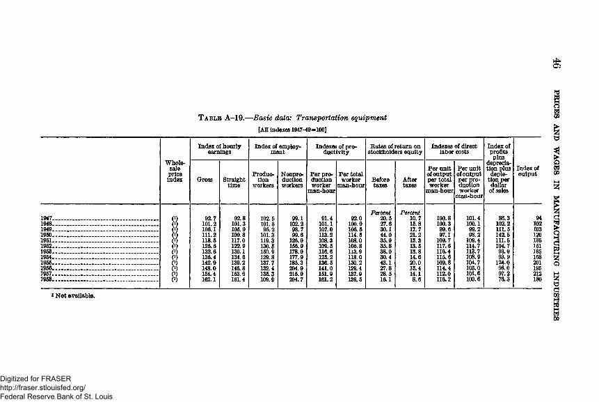
T able A - 19.— Basic data: Transportation equipment[All indexes 1947-49=.100]
Index of hourly earnings
Index of employment
Indexes of productivity
Rates of return on stockholders equity
Indexes of direct labor costs
Index of profits plus
Wholesalepriceindex Gross Straight
timeProduc
tionworkers
Nonproductionworkers
Per production worker
man-hour
Per total worker
man-hourBeforetaxes
Aftertaxes
Per unit of output per total worker
man-hour
Per unit of output per production worker
man-hour
depreciation plus
depletion per dollar
of sales
Index of output
1947............................................................... 0) 92.7 92.8 102.5 99.1 91.4 92.0Percent
20.5Percent
10.7 100.8 101.4 86.3 941948............................................................... 0) 101.2 101.3 101.3 102.2 101.1 100.9 27.6 15.8 100.3 100.1 102.2 1021949............................................................... (i) 106.1 105.9 96.2 98.7 107.0 106.5 30.1 17.7 99.6 99.2 111.5 1031950............................................................... 0) 111.2 109.8 101.3 99.6 113.2 114.5 44.0 21.2 97.1 98.2 142.5 1201951............................................................... 0) 118.5 117.0 119.3 126.9 108.3 108.0 35.9 13.3 109.7 109.4 111.5 135
0) 125.6 122.9 130.5 156.9 109.5 106.8 35.8 13.5 117.6 114.7 104.7 1511953............................................................... 0) 132.6 130.1 150.9 178.9 116.6 113.9 38.0 13.8 116.4 113.7 93.9 1851954............................................................... 0) 136.4 134.6 129.8 177.9 125.2 118.0 30.4 14.6 115.6 108.9 93.9 1681955............................................................... 0) 142.9 139.2 137.7 185.3 136.5 130.2 43.1 20.0 109.8 104.7 124.0 2011956............................................................... (l) 148.0 145.8 132.4 204.9 141.0 129.4 27.8 13.4 114.4 105.0 98.0 1951957............................................................... 0) 154.4 153.6 135.3 215.9 151.9 137.9 28.5 14.1 112.0 101.6 97.2 2121958............................................................... 0) 162.1 161.4 109.9 204.7 161.2 139.5 16.1 8.6 116.2 100.6 76.3 180
> Not available.
PRICES AND
WAGES
IN M
ANUFACTURING IN
DUSTRIES
Digitized for FRASER http://fraser.stlouisfed.org/ Federal Reserve Bank of St. Louis
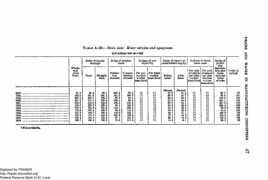
T a b l e A-20.— Basic data: Motor vehicles and equipment [AH indexes 1947-49*100]
Wholesalepriceindex
Index of hourly
Gross Straighttime
Index of employment
Production
workersNonproductionworkers
Per production worker
man-hour
Indexes of productivity
Per total worker
man-hour
Kates of return on stockholders equity
Beforetaxes
Aftertaxes
Per unit of output per total worker
man-hour
Indexes of direct labor costs
Per unit of output per production worker
man-hour
Index of profits plus
depreciation plus
depletion per dollar
of sales
Index of output
1947.. 1948-.1949..1950-1951-. 1952.1953-1954-1955.1956.1957. 1958-
91.3100.8107.9107.3112.9119.6118.9119.3122.9 129.8135.4139.7
92.3 101.0106.7111.7 119.9 128.0134.3137.4143.7147.5 154.4 160.0
92.1101.1106.8109.4119.6 126.0131.8135.6139.4145.8152.9159.9
100.4 101.398.3
108.6109.5 99.7
118.796.6
115.5100.3 97.5 74.3
98.9104.6 96.596.0
106.1113.2125.6 117.4122.2125.3121.3117.0
80)
0)0)0)<9(»)
Percent27.932.935.851.8 39.536.837.929.446.127.128.114.4
Percent15.618.720.924.614.113.613.613.921.113.014.0 8.1
90.7 9599.5 101
109.8 104137.1 132107.6 120105.4 10292.9 12695.8 109
126.8 153100.2 125102.5 12880.3 99
* Not available.
PRICES AND
WAGES
IN M
ANUFACTURING IN
DUSTRIES
Digitized for FRASER http://fraser.stlouisfed.org/ Federal Reserve Bank of St. Louis
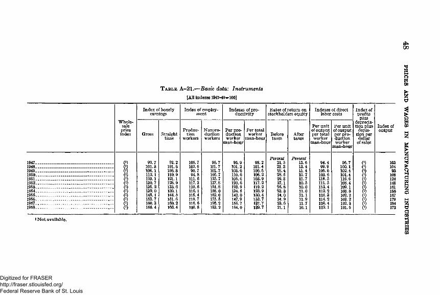
00
T a b l e A -2 1 .— Basic data: Instruments [All indexes 1947-49=100]
Wholesalepriceindex
Index of hourly earnings
Gross Straighttime
Index of employment
Production
workersNonproductionworkers
Per production worker
man-hour
Indexes of productivity
Per total worker
man-hour
Rates of return on stockholders equity
Beforetaxes
Aftertaxes
Per unit of output per total worker
man-hour
Indexes of direct labor costs
Per unit of output per production worker
man-hour
Index of profits plus
depreciation plus
depletion per dollar
of sales
Index of output
1947.1948.1949.1950.1951.1952.1953.1954.1955.1956.1957.1958.
92.7101.3106.1112.1123.1130.7135.2139.0145.1152.7160.3166.4
92.2101.6106.3110.9 121.1128.9 133.6139.1144.5151.6160.2166.4
106.7102.690.794.8 111.6
117.3125.6 116.1115.4118.7 116.6105.8
96.7101.7101.7106.7125.7137.8151.8158.0162.0 175.5 186.2 183.2
95.9 101.2103.6110.6105.6120.6123.9 134.5142.0147.9 156.7164.0
98.2101.4100.5108.2103.9117.2119.2123.9 130.4133.7137.7139.7
Percent21.521.318.428.529.3 27.125.823.324.024.923.621.1
Percent13.613.411.415.711.710.5 10.0 11.0 11.1 11.911.7 10.1
94.499.9
105.6103.6118.5111.5 113.4 112.2111.3 114.2116.4 119.1
96.7100.1102.4101.4 116.6108.4109.1 103.3102.2103.2102.3101.5 w(0
103104 93
108 124 148 161 156 167 179 184 173
PRICES AND
WAGES
IN M
ANU
FACTUR
ING
IN
DU
STRIE
S
Digitized for FRASER http://fraser.stlouisfed.org/ Federal Reserve Bank of St. Louis
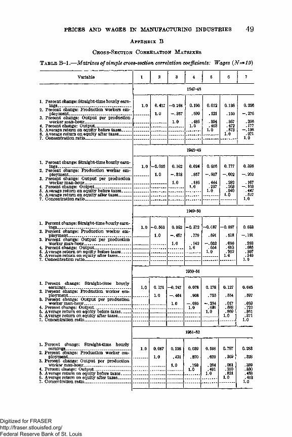
PRICES AND WAGES IN MANUFACTURING INDUSTRIES 49
A p p e n d ix B C r o s s -S e c t io n C o r r e l a t io n M a t r ix e s
T a b l e B -l .— Matrixes of simple cross-section correlation coefficients: Wages (N = 19 )
Variable 1 2 3 4 5 6 7
1947-48
1. Percent change: Straight-time hourly earnings............................................................
2. Percent change: Production workers employment____________________________
1.0 0.4171.0
-0.248-.357
0.195 .609
0.012.121
0.138 .150
0.226-.276
3. Percent change: Output per production worker man-hour_____________________ 1.0 .486 .394 .367 .396
4. Percent change: Output________________ 1.0 .463 .472 .1775. Average return on equity before taxes.. . . . 1.0 .873 -.1086. Average return on equity after taxes.......... 1.0 .0717. Concentration ratio....________ ________ 1.0
1948-49
1. Percent change: Straight-time hourly earnings_________________________________ 1.0 -0.050 0.162 0.024 0.616 0.777 0.336
2. Percent change: Production worker employment____________________________ 1.0 318 .857 -.057 -.002 -.202
3. Percent change: Output per production workerman-honr^ - ___________ 1.0 .186 .444 .282 .107
4. Percent «bangp.: Output.,,.. ..... 1.0 .237 .203 - . 1035. A v«rag« return nn equity hftfnra t vAs 1.0 .940 .4476. Average return on equity after taxes_____ 1.0 .5277. Concentration ratio_____________________ 1.0
1949-50
1. Percent change: Straight-time hourly earnings.............................................................
2. Percent change: Production worker employment____________________________
1.0 -0.563
1.0
0.362-.457
-0.372.779
-0 . C87 .591
-0.097.518
0.033-.191
3. Percent change: Output per production worker man-hour_____________________ 1.0 .142 -.052 .090 .293
4. Percent change: Output________________ 1.0 .654 .653 .0855. Average return on equity before taxes. _ __ 1.0 .902 .3076. Average return on equity after taxes______ 1.0 .3407. Concentration ratio_____________________ 1.0
1950-51
1. Percent change: Straight-time hourlyearnings......................................................
2. Percent change: Production worker employment____________________________
1.0 0.1711.0
-0.247—.464
0.078.908
0.178 .715
0.127 .554
0.045.597
3. Percent change: Output per production worker man-hour_________ ___________ 1.0 -.085 -.254 .017 .093
4. Percent change: Output.............................. 1.0 .631 .588 .7225. Average return on equity before taxes____ 1.0 .869 .3616. Average return on equity after taxes______ 1.0 .3717. Concentration ratio ___ __ 1.0
1951-52
1. Percent change: Straight-time hourlyearnings......................................................
2. Percent change: Production worker employment____________________________
1.0 0.0871.0
0.118.431
0.039.870
0.598
.620
0.707.369
0.283
.3283. Percent change: Output per production
worker man-hour_____________________ 1.0 .793 .284 .081 .3894. Percent change: Output..................... ........ 1.0 .491 .210 .3305. Average return on equity before taxes____ 1.0 .821 .4586. Average return on equity after taxes_____ 1.0 .4637. Concentration ratio_________________ 1.0
Digitized for FRASER http://fraser.stlouisfed.org/ Federal Reserve Bank of St. Louis
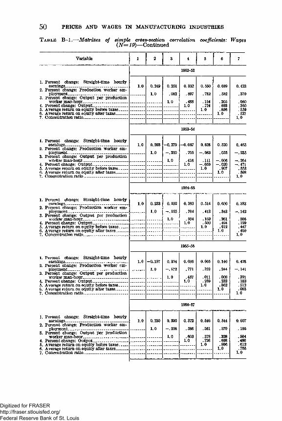
50 PRICES AND WAGES IN MANUFACTURING INDUSTRIES
T a b l e B -l.— Matrixes of simple cross-section correlation coefficients: Wages (N = 19)—Continued
Variable 1 2 3 4 5 6 7
1952-53
1. Percent change: Straight-time hourlyearnings......................................................
2. Percent change: Production worker employment
1.0 0.2491.0
0.251.082
0.332 .897
0.550 .782
0.689.582
0.423.370.080
3. Percent change: Output per production worker man-hour_____________________ 1.0 .488 .154 .205
4. Percent change: Output______ ____ _____ 1.0 .724 .603 .3605. Average return on equity before taxes____ 1.0 .806 .5596. Average return on equity after taxes_____ 1.0 .537
1.07. Concentration ratio_____________________
1953-54
1. Percent change: Straight-time hourlyearnings......................................................
2. Percent change: Production worker employment __________________________
1.0 0.2031.0
-0.279—.310
-0.067.705
0.628—.083
0.520.035
0.463—.235
3. Percent change: Output per production worker man-hour_____________________ 1.0 .416 .111 —.006 —.264
4. Percent change: Output________________ 1.0 —. 059 -.020 —.4715. Average return on equity before taxes____ 1.0 .907 .5536. Average return on equity after taxes______ 1.0 .5987. Concentration ratio ___________________ 1.0
1954-55
1. Percent change: Straight-time hourly earnings_____________________________ 1.0 0.233 0.102 0.383 0.514 0.600 0.383
2. Percent change: Production worker employment____________________________ 1.0 - . 155 .704 .413 .343 —. 142
3. Percent change: Output per production worker man-hour_____________________ 1.0 .504 .152 .261 .306
4. Percent change: Output_________________ 1.0 .500 .494 .1995. Average return on equity before taxes____ 1.0 .912 .4476. Average return on equity after taxes______ 1.0 .4607. Concentration ratio ___________________ 1.0
1955-56
1. Percent change: Straight-time hourlyearnings.....................................................
2. Percent change: Production worker employment _________________________
1.0 -0.197 1.0
0.354 -.172
0.086.771
0.055.323
0.146 .244
0.428 —. 141
3. Percent change: Output per production worker man-hour____________________ 1.0 .457 .011 .008 .391
4. Percent change: Output _______________ 1.0 .259 .232 .1825. Average return on equity before taxes____ 1.0 .862 .5126. Average return on equity after taxes ___ 1.0 .6037. Concentration ratio __________________ 1.0
1956-57
1. Percent change: Straight-time hourlyearnings_____________________________
2. Percent change: Production worker employment____________________________
1.0 0.230
1.0
0.390
-.258
0.372
.586
0.546.561
0.544.570
0.607.186
3. Percent change: Output per production worker man-hour_____________________ 1.0 .603 .378 .328 .504
4. Percent change: Output _______________ 1.0 .726 .698 .4805. Average return on equity before taxes____ 1.0 .906 .6126. Average return on equity after taxes_____ 1.0 .7557. Concentration ratio_____________________ 1.0
Digitized for FRASER http://fraser.stlouisfed.org/ Federal Reserve Bank of St. Louis
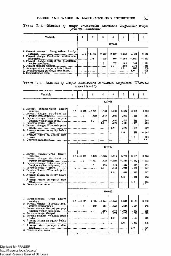
PRICES AND WAGES IN MANUFACTURING INDUSTRIES 51
T a b l e B-l.— Matrixes of simple cross-section correlation coefficients: Wages (iV=19)—Continued
Variable 1 2 3 4 5 6 7
1957-58
1. Percent change: Straight-time hourly earnings______________________________ 1.0 -0.576 0.049 -0.440 0.392 0.484 0.549
2. Percent change: Production worker employment____________________________ 1.0 .079 .880 -.009 -.030 -.532
3. Percent change: Output per production worker man-hour_____________________ 1.0 .527 .462 .359 .121
4. Percent change: Output________________ 1.0 .222 .171 —.3495. Average return on equity before taxes____ 1.0 .883 .5066. Average return on equity after taxes______ 1.0 .6987. Concentration ratio_____________________ 1.0
T a b l e B-2.— Matrixes of simple cross-section correlation coefficients: Wholesale prices (N =16 )
Variable 1 2i
3 4 5 6 7 8
1947-48
1. Percent change: Gross hourlyearnings.______ ______________
2. Percent change: P ro d u c t io nworker employment__________
1.0 0.4231.0
-0.361 -.439
0.188 .647
0.093.291
0.029.089
0.107.110
0.333-.161
3. Percent change: Output per production worker man-hour_____ 1.0 .369 .024 .404 .383 .356
4. Percent change: Output.............. 1.0 .375 .438 .458 .2065. Percent change: Wholesale price
index______________ ________ 1.0 .339 .560 .3296. Average return on equity before
taxes__________ ______ _____ 1.0 .888 -.1047. Average return on equity after
taxes______________ _____ 1.0 .1398. Concentration ratio. - _____ 1.0
1948-49
1. Percent change: Gross hourlyearnings_____________________
2. Percent change: P ro d u c t io nworker employment__________
1.0 -0.191 1.0
0.152 -.421
-0.106 .832
0.214-.520
0.767-.333
0.888-.239
0.595 - . 125
3. Percent change: Output per production worker man-hour_____ 1.0 .133 .328 .534 .295 .172
4. Percent change: Output________ 1.0 -.416 -.045 -.074 -.0375. Percent change: Wholesale price
index_____ _____ _ _ _ . 1.0 .439 .335 .2876. Average return on equity before
taxes____ _______ _______ . . . . 1.0 .927 .4667. Average return on equity after
taxes______ 1.0 .6158. Concentration ratio__ ________ 1.0
1949-50
1. Percent change: Gross hourlyearnings_____________________
2. Percent change: P ro d u c t io nworker employment__________
1.0 -0.3711.0
0.303-.489
-0.151 .781
-0.055-.050
0.087.735
0.126.595
0.033-.246
3. Percent change: Output pel production worker man-hour.. 1.0 .104 .170 -.092 .097 .288
4. Percent change: Output 1.0 .073 .776 .752 -.0135. Percent change: Wholesale price
index___ _ . . . 1.0 -.041 .113 —.0196. Average return on equity before
taxes..... ... ............... 1.0 .907 .1387. Average return on equity after
taxes____ . . . 1.0 . 2568. Concentration ratio. 1.0
Digitized for FRASER http://fraser.stlouisfed.org/ Federal Reserve Bank of St. Louis
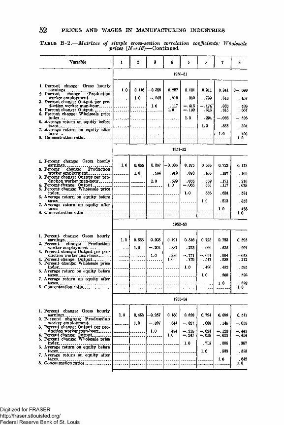
52 PRICES AND WAGES IN MANUFACTURING INDUSTRIES
T a b l e B -2.— Matrixes of simple cross-section correlation coefficients: Wholesale prices (N = 16)—Continued
Variable 1 2i
3 4 5 6 7 8
1. Percent change: Gross hourly earnings___ -
1960-51
1.0 0.4161.0
—0.389-.2681.0
0.287.912
.1171.0
0.101.052
-.415-.1991.0
0.311
.733—. 174*
.616
.2941.0
0.341
.616
.083
.615-.066
.8851.0
0 - . 099.457.409.667
-.526.304
.4091.0
2. Percent change :Production worker employment__________
3. Percent change: Output per production worker man-hour______
4. Percent change: Output________5. Percent change: Wholesale price
index_______________________6. Average return on equity before
taxes________ ____ ___________7. Average return on equity after
taxes________________ ______8. Concentration ratio.................. .
1. Percent change: Gross hourly earnings,_ „ _
1951-52
1.0 0.0551.0
0.007.594
1.0
-0.036.912
.8291.0
0.375.093.035
-.0651.0
0.656.450.362.365.536
1.0
0.723.197.171.117.624.813
1.0
0.173.169.216.073.581.358.488
1.0
2. Percent change: Production worker employment__________
3. Percent change: Output per production worker man-hour_____
4. Percent change: Output________5. Percent change: Wholesale price
index_____________ ___ _______6. Average return on equity before
taxes_____________________7. Average return on equity after
taxes_________________________8. Concentration ratio_______ _____
1. Percent change: Gioss hourly earnings_____________________
1952-53
1.0 0.3831.0
0.203-.2041.0
0.491.837.336
1.0
0.546.275
- . 171 .176
1.0
0.725.666
-.094.547.490
1.0
0.783.525.094.538.432.800
1.0
0.595.201
-053.212.595.523.622
1.0
2. Percent change: Production worker employment.... ...........
3. Percent change: Output per production worker man-hour........ .
4. Percent change: Output________5. Percent change: Wholesale price
index_________ ______________6. Average return on equity before
taxes________________________7. Average return on equity after
taxes________ _____ __________8. Concentration ratio_______ _____
1. Percent change: Gross hourly earnings______________________
1953-54
1.0 0.458
1.0
-0.257-.327
1.0
0.160.644
.4741.0
0.620
-.027-.215-.2471.0
0.794
.088-.023-.018
.7151.0
0.699
.145- . 123 -.023
.505
.8881.0
0.517
-.058-.443-.454
.387
.515
.6421.0
2. Percent change: Production worker employment__________
3. Percent change: Output per production worker man-hour______
4. Percent change: Output_________5. Percent change: Wholesale price
index________________________6. Average return on equity before
taxes_________________________7. Average return on equity after
taxes______________________ __8. Concentration ratios____________
Digitized for FRASER http://fraser.stlouisfed.org/ Federal Reserve Bank of St. Louis
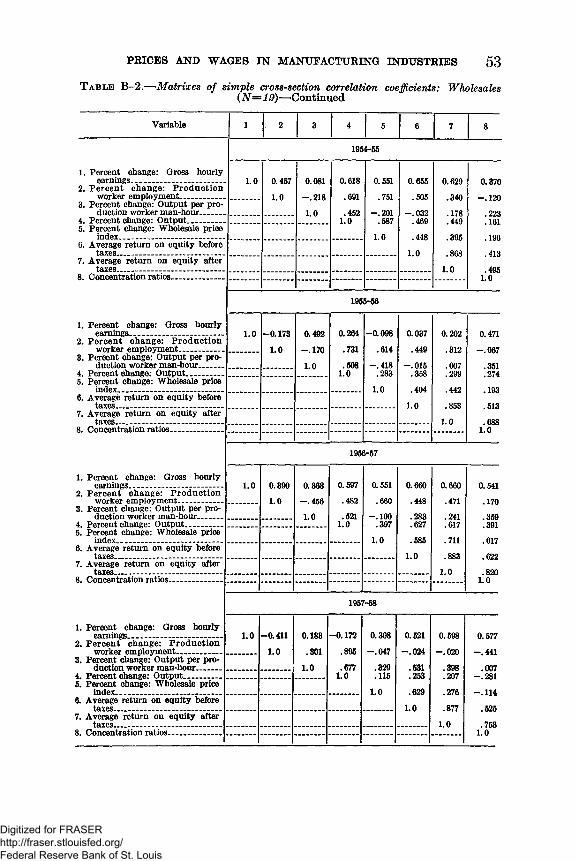
PRICES AND WAGES IN MANUFACTURING INDUSTRIES 5 3
T a b l e B-2.— Matrixes of simple cross-section correlation coefficients: Wholesales (N = 19 )—Continued
Variable 1 2 3 4 5 6 7 8
1. Percent change: Gross hourlyearnings........................................
2. Percent change: Productionworker employment-.................
1954-55
1.0 0.4571.0
0.081-.2181.0
0.618.691
.4521.0
0.551.751
-.201.587
1.0
0.655.505
-.032.469.448
1.0
0.629.340.178.449
.395
.8681.0
0.370- . 120
.223
.161
.196
.413
.4951.0
3. Percent change: Output per production worker man-hour..........
4. Percent change: Output................5. Percent change: Wholesale price
index________________________6. Average return on equity before
taxes_________________________7. Average return on equity after
taxes_________________________8. Concentration ratios____________
1. Percent change: Gross hourly earnings______________________
1955-56
1.0 -0.1731.0
0.492-.1701.0
0.264
.731
.5081.0
-0.098.614
-.418.283
1.0
0.037.449
-.015.358.404
1.0
0.202.312.007.299.442
.8531.0
0.471-.067
.351
.274
.193
.513
.6881.0
2. Percent change: Productionworker employment...................
3. Percent change: Output per production worker man-hour_____
4. Percent change: Output________5. Percent change: Wholesale price
index________________________6. Average return on equity before
taxes_________________________7. Average return on equity after
taxes_________________________8. Concentration ratios____________
1. Percent change: Gross hourly earnings______________________
1956-57
1.0 0.3901.0
0.368-.4561.0
0.597.482.521
1.0
0.551.660
- . 100 .397
1.0
0.660.448.283.627.585
1.0
0.660.471.241.617.711.883
1.0
0.541.170.359.391.617.622.820
1.0
2. Percent change: Production worker employment__________
3. Percent change: Output per production worker man-hour______
4. Percent change: Output________5. Percent change: Wholesale price
index________________________6. Average return on equity before
taxes_________________________7. Average return on equity after
taxes_________________________8. Concentration ratios____________
1. Percent change: Gross hourlyftarningfi_____________________
1957-58
1.0 —0.411 1.0
0.183.301
1.0
-0.172.895.677
1.0
0.308-.047
.329
.115
1.0
0.521-.024
.531
.253
.629
1.0
0.598-.020
.398
.207
.276
.8771.0
0.577-.441
.007-.281-.114
.525
.7531.0
2. Percent change: Production worker employment__________
3. Percent change: Output per production worker man-hour______
4. Percent change: Output_________5. Percent change: Wholesale price
index________________________6. Average return on equity before
taxes_________________________7. Average return on equity after
taxes________________________8. Concentration ratios___ -___ -__ -
Digitized for FRASER http://fraser.stlouisfed.org/ Federal Reserve Bank of St. Louis
In order to compare the movements of prices, wages, labor costs, and returns to capital in each 2-digit manufacturing industry, indexes were computed showing the ratio between the index of these variables in each industry and the index of the same variables in all manufacturing. The resulting indexes are presented in tables C -l to 0-20. A brief description of each of them follows.„ txt, i i . r j Wholesale Price Index: Industry1. Wholesale Price Index \—=ft — =r~ ------ irr-----5—I— :—Wholesale Price Index: Manufacturing
The basic wholesale price indexes are given in appendix A.Index of Straight Time Hourly Earnings:
2 . Straight Time Hourly E a r n i n g s ^ Ti me Hourly Earnings:Manufacturing
n . Index of Output: Industry Uutput” Index of Output: Manufacturing
The basic indexes of output are given in appendix A.Index of Output per Total Worker
4. Output Per Total Worker Man-Hour = T ^ an : — —Index of Output per Total WorkerMan-Hour: Manufacturing
The basic indexes of output per total worker man-hour are given in appendix A.5. Direct Labor Costs Per Unit of Output Per Total Worker Man-Hour
Index of Direct Labor Costs/Unit of Output/TWMH: Industry_____""Index of Direct Labor Costs/Unit of Output/TWMH: Manufacturing
Direct labor costs were measured by the index of gross hourly earnings of production workers; no data are available for hourly costs of both production and nonproduction workers. As a result, the index of direct labor costs probably understates the rate of increase in total labor costs, since nonproduction workers have increased considerably faster than production workers and since the average hourly compensation rate for nonproduction workers is probably higher than the average gross hourly earnings of production workers.
Index of Profits Plus Depreciation Plus ~ ~ -i ii c i Depletion Per Dollar of Sales: Industry
0 . Capital Costs Per Dollar of Sales= 7 —5— ^ ------- r-r.---- ™-----* Index of Profits Plus Depreciation PlusDepletion Per Dollar of Sales: Manufacturing
The basic indexes of profits plus depreciation plus depletion per dollar of sales are given in appendix A.
It should be noted that the same limitations discussed in appendix A with regard to comparability of scope and classification method are applicable in equal degree to the data presented here. It should also be noted that one important part of costs—viz, costs of materials per unit—are not available. In a few instances, indirect taxes may also represent a fairly important part of the final price not accounted for by the costs included above.
Tables C -l to C-2 0 follow.
A p p e n d i x C
T r e n d s i n I n d i v i d u a l I n d u s t r i e s R e l a t i v e t o A l l M a n u f a c t u r i n g
54
Digitized for FRASER http://fraser.stlouisfed.org/ Federal Reserve Bank of St. Louis
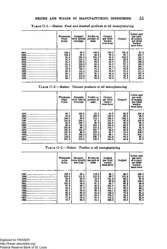
1947.1948.1949.1960.1951.1952.1953.1954.1955.1956.1957.1958.
1947.1948.1949.1950.1951.1952.1953.1954.1955.1956.1957.1958.
1947.1948.1949.1950.1951.1952.1953.1954.1955.1956.1957.1968.
PRICES AND WAGES IN MANUFACTURING INDUSTRIES 55
T a b le 0 -1 .— Ratios: Food and kindred products to all manufacturing
WholesalePriceIndex
Straight time hourly
earningsProfits as percent of
Output per total worker
man-hourOutput
Labor cost per unit of output per total worker
man-hour
102.4102.295.4 95.996.596.4 92.792.688.485.185.789.1
100.4 101.6 100.8 102.2 102.0103.1104.5 103.7104.2 105.0
109.889.3 101.286.693.886.590.3 91.084.6 91.5 90.2
102.298.898.895.495.896.494.495.7 92.694.896.298.2
101.096.1
103.092.8 87.587.181.388.882.3 82.8 82.8 91.0
97.9100.7101.5105.2103.8104.5 106.7106.6111.2107.9107.2106.3
Table 0 -2 .—Ratios: Tobacco products to all manufacturing
WholesalePriceIndex
Straight time hourly
earningsProfits as percent of
salesOutput
per total worker
man-hourOutput
99.7 102.0 85.1 95.8 98.096.0 98.6 102.0 100.0 98.1
104.6 99.6 114.1 104.5 104.1102.8 103.1 97.3 101.9 91.995.6 100.7 98.9 106.6 90.098.6 99.2 102.4 106.3 90.3
105.6 99.1 116.3 103.7 82.1106.2 101.0 120.7 98.0 84.0105.0 99.2 119.1 93.7 76.6101.3 103.2 125.3 98.1 76.6102.6 103.7 138.7 104.6 79.3105.2 104.8 159.8 114.6 91.8
Labor cost per unit of output per total worker
man-hour
106.498.695.2
100.693.592.594.8
102.7 106.0 104.198.491.9
Table C-3.—Ratios: Textiles to all manufacturing
Wholesalepriceindex
Straight- time hourly
earningsProfits as percent of
salesOutput
per total worker
man-hourOutput
Labor cost per unit of output per total worker
man-hour
103.4102.094.697.2
100.387.684.680.780.276.7 74.370.7
99.1 101.399.699.5 98.896.191.288.686.386.3 84.5 82.2
113.2110.373.979.567.548.253.539.949.955.2 51.864.5
98.799.7
101.998.399.7 101.6
101.1104.1103.0105.0105.2108.2
99.0 101.999.098.288.3 84.779.980.078.0 76.673.176.9
100.2101.597.8
100.998.694.3 90.184.784.4 82.0 81.0 77.0
Digitized for FRASER http://fraser.stlouisfed.org/ Federal Reserve Bank of St. Louis
56 PRICES AND WAGES IN MANUFACTURING INDUSTRIES
Table C-4.—Ratios: Apparel to all manufacturing
Wholesalepriceindex
Straight- time hourly
earningsProfits as percent of
salesOutput
per total worker
man-hourOutput
Labor cost per unit of output per total worker
man-hour
105.0 104.1 134.0 101.7 97.0 102.699.4 100.3 88.7 100.2 99.0 100.295.8 96.1 75.3 97.9 104.1 97.892.9 94.5 78.2 95.6 97.3 98.3
1951........................................... 90.4 94.7 58.6 94.2 88.3 98.989.6 89.3 77.8 93.5 89.5 95.689.2 86.0 82.3 90.3 84.3 95.588.0 86.1 79.2 86.8 87.2 98.587.2 82.1 80.2 89.6 85.1 92.085.1 84.0 94.6 88.9 83.4 94.582.6 82.1 83.4 87.3 82.1 94.681.6 80.5 80.9 88.9 87.3 91.4
Table C--5.—Ratios: Lumber to all manufacturing
Wholesalepriceindex
Straight time hourly
earningsProfits as percent of
salesOutput
per total worker
man-hourOutput
Labor cost per unit of output per total worker
man-hour
1947 ..................................... 97.7 100.5 116.6 97.9 101.0 102.31948........................................... 103.3 100.3 100.5 102.4 101.9 97.91949........................................... 98.9 99.3 81.1 98.6 95.9 100.91950 .......................................... 109.4 101.5 92.4 101.4 100.9 99.41951...................... ................... 107.3 102.4 87.7 97.4 93.3 103.81952 ........................... ......... 106.6 102.2 76.1 99.3 88.7 102.31953 ................- ....................... 106.6 101.4 70.4 103.6 85.1 96.71954......................... .................. 103.8 99.0 73.1 107.6 88.8 91.51955........................................... 107.5 98.3 85.2 105.2 87.2 93.01956 ..................................... 104.9 97.6 68.2 102.8 82.1 94.61957........................................... 96.6 96.1 58.0 105.0 75.2 91.21958........................................... 94.5 96.6 72.5 109.6 82.1 88.5
Table 0—6.—Ratios: Furniture and fixtures to all manufacturing
Wholesalepriceindex
Straight time hourly
earningsProfits as percent of
salesOutput
per total worker
man-hourOutput
Labor cost per unit of output per total worker
man-hour
1947 .......................................... 99.4 99.9 113.7 101.0 100.0 99.31948 .......................................... 98.6 100.1 103.2 99.8 101.0 100.11949........................................... 102.0 100.1 81.2 99.0 99.0 100.71950 .......................................... 102.3 99.1 89.2 94.9 105.4 104.31951.......................................... 102.8 99.7 89.6 94.1 92.5 105.31952 .......................................... 102.7 99.8 84.7 93.5 91.9 106.61953........................................... 103.8 99.3 81.6 92.2 88.8 106.91954 .......................................... 103.1 99.0 73.4 103.4 99.2 94.81955........................................... 103.7 97.7 73.9 101.5 100.0 96.11956 .......................................... 105.1 97.8 84.5 100.4 100.0 96.31957........................................... 106.0 96.4 76.9 97.1 95.9 98.51958........................................... 106.1 94.8 73.8 96.3 98.5 98.3
Digitized for FRASER http://fraser.stlouisfed.org/ Federal Reserve Bank of St. Louis
PRICES AND WAGES IN MANUFACTURING INDUSTRIES
T a b le C -7 .— Ratios: Paper and products to all manufacturing
57
WholesalePriceIndex
Straight time hourly
earningsProfits as percent of
Output per total worker
man-hourOutput
Labor cost per unit of output per total worker
man-hour
1947.1948.1949. 1960. 1951.19521953 1954.195519561957.1958.
102.899.198.2 96.9
103.5103.2 102.9102.3 103.7106.4105.2105.2
98.4100.5 101.0100.6100.7101.8 100.2 101.5 101.8 103.1 103.3 104.0
116.493.489.392.6
106.7102.895.696.2 88.1 89.883.487.3
102.199.698.2
100.8 102.697.297.397.6 99.1 99.097.7
101.7
100.099.0 101.0
106.3104.296.097.0
105.6105.7 107.6 106.9117.2
96.8 100.8102.4100.497.9
104.3103.1103.8103.1103.9105.9 102.7
T a b l e C-8.— Ratios: Printing and publishing to all manufacturing
WholesalePriceIndex
Straight time hourly
earningsProfits as percent of
salesOutput
per total worker
man-hourOutput
Labor cost per unit of output per total worker
man-hour
194719481949195019511952195319541955195619571958
0)(>)0)0)0)(00)0)C1)0)0)0)
96.999.8
103.0102.899.2 99.698.398.598.496.6 95.295.4
108.194.297.581.3 94.798.298.396.689.694.494.6 95.3
99.8 100.399.595.596.9 92.891.192.389.189.487.485.6
96.098.1
106.297.391.788.785.896.090.192.492.497.8
97.399.4
103.3106.7 101.1 106.1106.7106.3109.9106.9 108.1 111.0
i Not available.
T a b l e C-9.— Ratios: Chemicals to all manufacturing
Wholesalepriceindex
Straight time hourly
earningsProfits as percent of
salesOutput
per total worker
man-hourOutput
Labor cost per unit
of output per total worker
man-hour
1947 _________ ____________ 105.7 98.9 97.9 96.8 96.0 102.11948.............................. ........... 100.0 99.6 95.4 99.6 100.0 100.01949.................. ...................... 94.5 101.4 107.4 103.5 104.1 97.91950_________________ ______ 92.5 102.9 112.3 111.6 111.7 91.81951____ _____ _______ _____ _ 95.2 102.3 112.6 114.6 115.8 88.81952 _____________________ 92.6 102.9 115.9 113.3 116.1 89.81953________ _____ __________ 91.8 103.3 116.9 111.9 114.9 91.81954..................... ............... . 94.1 104.9 118.0 111. 1 122.4 94.21955 ________ ____ ________ 92.7 105.3 119.1 118.5 126.2 88.81956..................... ..................... 89.7 106.7 116.7 121.5 131.7 87.11957 ___________ ____ _____ 88.9 106.9 120.8 122.7 137.2 86.71958 __________________ ___ 88.7 107.6 122.5 125.0 148.5 86.1
50505 0— 60-------5Digitized for FRASER http://fraser.stlouisfed.org/ Federal Reserve Bank of St. Louis
58 PRICES AND WAGES IN MANUFACTURING INDUSTRIES
T a b l e C - 1 0 .— Ratios: Petroleum and products to all manufacturing
Wholesalepriceindex
Straight time hourly
earningsProfits as percent of
salesOutput
per total worker
man-hourOutput
Labor cost per unit of output per total worker
man-hour
1947 _____________________ 93.4 97.0 98.2 101.6 97.0 95.11948________________________ 108.0 100.9 105.3 101.4 101.0 99.31949 _____________________ 98.0 102.0 95.9 95.8 101.0 106.81950________________________ 106.7 100.2 85.2 100.9 99.1 99.21951________________________ 94.7 99.9 93.5 106.3 101.7 93.71952________ ____ ___________ 98.5 100.5 94.5 102.8 97.6 97.41953 _____________________ 99.2 100.2 96.5 103.1 96.3 96.91954 _____________________ 95.9 100.1 97.1 98.6 98.4 101.71955________________________ 96.7 100.3 89.5 101.9 95.7 98.51956________________________ 98.3 102.7 93.7 103.9 96.6 98.81957______________ _____ ___ 102.1 102.0 90.7 102.6 95.9 99.71958_________________ ______ 92.2 102.4 91.7 100.5 97.0 102.3
T a b l e C - l l . — Ratios: Rubber and products to all manufacturing
Wholesalepriceindex
Straight time hourly
earningsProfits as percent of
salesOutput
per total worker
man-hour
OutputLabor cost
per unit of output per total worker
man-hour
1947______ ____ ____________ 102.2 103.1 106.7 100.9 106.0 102.01948________________________ 98.1 99.1 100.1 100.3 99.0 98.41949_______________ ____ ___ 99.9 98.3 92.4 99.9 95.9 98.71950___ ___________ ____ ___ 107.6 97.5 107.2 99.4 100.0 99.11951________________________ 114. 7 97.2 118.4 98.0 96.7 99.41952___ ______________ _____ 113.7 99.8 113.6 95.2 94.4 105.51953___ ____________________ 111.4 99.2 109.5 96.1 94.0 103.91954________________________ 112.3 99.0 109.3 99.3 94.4 100.31955______ _________________ 121.9 99.7 103.1 96.4 97.9 105.61956.......................... ......... ...... 121.8 100.2 106.4 94.0 91.0 106.81957______ ________________ _ 118.9 98.9 108.7 93.1 91.0 107.31958___ _____ _____ _________ 119.0 100.4 117.8 94.7 91.8 106.7
T a b l e C -1 2 .— Ratios: Leather and products to all manufacturing
WholesalePriceIndex
Straight time hourly
earningsProfits as percent of
salesOutput
per total worker
man-hour
OutputLabor cost per unit
of output per total worker
man-hour
1947________________________ 103.8 102.6 124.3 103.8 105.0 98.71948___ __________________- 98.4 100.1 94.0 98.8 97.1 101.11949____ ____________ ______ 98.1 97.7 79.8 97.3 97.9 100.61950________________________ 100.8 98.6 95.7 96.2 93.7 101.31951_________________ ______ 104.3 97.4 74.5 98.8 80.8 97.41952_____ ___________ ______ 91.9 96.3 106.6 95.3 83.9 100.11953_____ ________________- 92.5 94.1 109.4 92.6 77.6 100.81954_____ __________________ 89.4 92.1 116.2 95.1 82.4 96.51955________________________ 88.2 91.1 117.8 92.1 79.4 98.11956__________________ ____ - 89.9 91.8 93.8 93.4 78.6 97.21957________________________ 87.7 90.2 102.1 93.7 77.9 95.71958____________________ 87.6 88.9 102.4 93.5 81.3 95.0
Digitized for FRASER http://fraser.stlouisfed.org/ Federal Reserve Bank of St. Louis
PRICES AND WAGES IN MANUFACTURING INDUSTRIES 59
T able C -13.— Ratios: Stone, clay, and glass products to all manufacturing
Wholesalepriceindex
Straight time hourly
earningsProfits as percent of
Output per total worker
man-hourOutput
Labor cost per unit of output per total worker
man-hour
1947.1948.1949.1950.1951.1952.1953.1954. 19551956.1957.1958.
96.797.4
105.2105.0 101.6104.6109.6112.0114.3116.3 117.5 120.1
99.599.7
100.9 101.1 100.299.8
100.6 100.7101.9 102.0 102.1 101.6
92.596.9
111.9110.7111.5110.5 110.2113.8113.3116.9117.3 125.2
100.5 100.498.9
102.3105.3102.6 99.6 99.8 99.0 99.4 99.2
100.1
99.0 101.0 100.0105.4107.5 99.294.097.698.6
100.098.6
100.7
99.099.3101.898.994.996.9
100.7100.9 103.0102.7102.9 102.5
T a b l e C-14.— Ratios: Primary metals to all manufacturing
Wholesalepriceindex
Straight time hourly
earningsProfits as percent of
Output per total worker
man-hour
OutputLabor cost
per unit of output per total worker
man-hour
1947.1948.1949.1950.1951.1952.1953.1954.1955. 19561957.1958.
94.399.0
106.5107.3107.2 110.8117.3 119.7 126.1 132.1132.3 131.9
99.599.7100.899.3
100.3100.9102.7102.8104.8105.8 107.1110.8
95.2100.1105.1108.2113.0 97.1112.8112.2
116.0115.3 112.9110.4
102.1 100.996.899.498.894.496.8 91.096.9 92.289.9 84.7
103.0103.992.8
102.7 104.291.197.084.897.293.1 89.776.1
97.499.0
103.8100.4 102.2107.0 106.6112.4109.1 114.6119.2 130.1
T a b l e C-15.— Ratios: Fabricated metal products to all manufacturing
Wholesalepriceindex
Straight time hourly
earningsProfits as percent of
salesOutput
per total worker
man-hourOutput
Labor cost per unit of output per total worker
man-hour
1947________________________ 94.7 99.2 107.1 100.4 102.0 99.11948----- ------ ----------------------- 98.7 99.6 99.7 100.5 101.0 99.31949........................................... 106.4 101.1 92.4 98.1 95.9 102.61950..-..................................... 106.1 100.5 95.5 97.6 102.7 103.41951............. — -------------------- 105.3 99.7 99.2 95.3 100.8 105.11952___ ____________________ 106.8 100.2 87.7 91.4 94.4 110.11953____ ___________________ 108.5 100.0 81,1 91.2 98.5 110.61954............................ ........... - 109.1 101.0 74.0 88.8 95.2 114.01955________________________ 111.3 100.9 74.6 85.2 92.2 119.41956_________________ ____ - 113.8 101.1 73.1 83.4 89.7 121.01957____ _____ - ........- ........- 115.1 101.5 74.1 83.4 91.7 121.81958........ ............................... - 114.5 102.7 75.6 84.1 91.0 122.2
Digitized for FRASER http://fraser.stlouisfed.org/ Federal Reserve Bank of St. Louis
T a b l e C-16.— Ratios: Machinery, except electrical, to all manufacturing
60 PRICES AND WAGES IN MANUFACTURING INDUSTRIES
Wholesalepriceindex
Straight time hourly
earnings
Profits as percent of
salesOutput
per total worker
man-hourOutput
Labor cost per unit of output per total worker
man-hour
1947________________ _______ 96.4 100.2 100.9 101.0 104.0 99.01948__________ ______ _______ 97.4 99.3 97.5 100.1 102.9 99.61949____ ___________________ 106.3 100.6 101.8 98.9 92.8 101.21950______________________ 105.9 100.5 96.7 98.4 92.8 102.31951........................................... 106.1 100.1 103.8 98.5 104.2 103.01952________________________ 109.0 101.4 104.3 99.4 107.3 102.91953........ ................................. 111.4 100.9 93.1 99.2 103.7 102.41954.................... ....................... 112.4 102.2 91.5 93.9 95.2 108.51955________________________ 115.9 101.4 89.4 91.1 90.8 112.01956________________ _______ 120.7 102.4 97.3 91.2 98.6 112.21957___ ___________ ________ 124.6 102.4 96.2 86.0 93.1 118.51958________________________ 126.2 103.4 95.0 84.8 85.1 120.8
T a b l e C-17.— Ratios: Electrical machinery to all manufacturing
WholesalePriceIndex
Straight time hourly
earningsProfits as percent of
salesOutput
per total worker
man-hourOutput
Labor cost per unit of output per total worker
man-hour
1947......................................... 100.4 100.2 99.2 98.2 103.0 101.81948______________ _________ 97.8 99.9 96.7 99.6 99.0 100.31949.................. ........... ............. 101.9 100.0 104.6 102.7 97.9 97.41950________________________ 99.6 97.3 116.0 100.0 104.5 97.91951__________________ _____ 100.6 97.0 111.9 97.3 107.5 100.01952 _____________________ 103.6 97.7 112.5 106.6 125.8 91.81953________________________ 106.7 97.1 102.7 103.1 129.9 94.51954________________________ 105.8 98.2 95.4 105.1 127.2 93.51955_______ ________________ 107.3 97.6 82.9 104.5 124.8 93.71956 _____________________ 111.5 98.1 79.8 105.9 134.5 92.41957 _______ ______ _______ 113.4 98.1 92.3 104.0 135.2 94.11958. _____________________ 113.0 99.0 95.0 99.1 128.4 99.7
T a b l e C-18.— Ratios: Transportation equipment to all manufacturing
1947.1948.1949.1950.1951.1952.1953.1954.1955. 19561957.1958.
WholesalePriceIndex
Straight time hourly
earningsProfits as percent of
salesOutput
per total worker
man-hourOutput
0) 100.1 84.4 95.1 94.0(l) 99.9 97.3 100.9 99.00) 100.1 120.3 102.7 106.20) 100.3 119.7 103.7 108.1(0 98.7 97.3 98.6 112.50) 98.6 105.0 94.9 121.80) 98.3 93.3 98.1 138.10) 98.8 95.8 99.2 134.4(0 98.8 109.9 103.3 142.60) 98.6 89.7 100.6 134.50) 98.7 95.0 105.2 146.20) 100.2 82.3 104.8 134.3
Labor cost per unit of output per total worker
man-hour
104.798.798.097.3
100.5 105.4101.6101.0 97.998.894.3 96.5
1 Not available.
Digitized for FRASER http://fraser.stlouisfed.org/ Federal Reserve Bank of St. Louis
PRICES AND WAGES IN MANUFACTURING INDUSTRIES 61
T a b l e C-19.— Ratios: Motor vehicles and equipment to all manufacturing
Wholesalepriceindex
Straight time hourly
earningsProfits as percent of
salesOutput
per total worker
man-hourOutput
Labor cost per unit of output per total worker
man-hour
1947............................................ 95.2 99.4 88.7 0) 95.0 (01948............................................ 97.1 99.7 94.8 0) 98.0 (01949............................................ 107.6 100.9 118.4 0) 107.2 0)1950............................................ 103.0 99.9 115.2 0) 117.9 - 0)1951............................................ 97.7 100.9 93.9 0) 100.0 0)1952............................................ 105.9 101.1 105.7 0) 81.6 0)1953............................................ 105.4 99.5 92.3 (0 92.6 (01954............................................ 104.9 99.5 97.8 0) 85.8 (l)1955............................................ 106.9 98.9 112.4 0) 107.7 0)1956............................................ 108.6 98.6 91.7 (0 85.0 0)1957............................................ 109.9 98.3 100.2 0) 87.1 0)1958........................................... 112.2 99.3 86.6 (*) 72.8 0)
i Not available.
T a b l e C-20.— Ratios: Instruments and related products to all manufacturing
Wholesalepriceindex
Straight time hourly
earningsProfits as percent of
salesOutput
per total worker
man-hourOutput
Labor cost per unit of output per total worker
man-hour
1947-— ..................................... (0 99.5 0) 101.6 103.0 98.01948........................................... 0) 100.2 (0 101.4 101.0 98.31949........................................... (0 100.5 0) 96.9 95.9 103. S1950........................................... 0) 101.3 (0 98.0 97.3 103.81951........................................... (0 102.2 0) 94.9 103.3 108.51952........................................... (0 103.5 0) 104.2 119.4 99.81953........................................... <0 100.9 0) 102.7 120.1 99.01954........................................... 0) 102.1 (0 104.1 124.8 98.01955........................................... 0) 102.6 0) 103.4 118.4 99.31956........................................... 0) 102.5 0) 104.0 123.4 98.61957........................................... 0) 103.0 0) 105.0 126.9 98.01958........................................... 0) 103.4 0) 105.0 129.1 98.9
i Not available.
Digitized for FRASER http://fraser.stlouisfed.org/ Federal Reserve Bank of St. Louis

Digitized for FRASER http://fraser.stlouisfed.org/ Federal Reserve Bank of St. Louis
TECHNICAL NOTE NO. 1 THE SERVICE SECTOR: DATA ON OUTPUT,
EMPLOYMENT, PRICES, AND INCOME
(By George W. Bleile)
63
Digitized for FRASER http://fraser.stlouisfed.org/ Federal Reserve Bank of St. Louis

Digitized for FRASER http://fraser.stlouisfed.org/ Federal Reserve Bank of St. Louis

THE SERVICE SECTOR: DATA ON OUTPUT, EMPLOYMENT, PRICES, AND INCOMES
By George W. BleileThe purpose of this note is to present more fully some of the data which were
developed during the investigation of inflation and growth in the service sector. The major findings ha\e been reported in chapters 3 and 5 of the Joint Economic Committee “ Staff Report on Employment, Growth, and Price Levels” (Washington, 1959).
The note is in three parts. Part 1 contains data on an aggregate basis for the entire service sector including finance and insurance, transportation, utilities, professional and other personal services. The second part presents more specific data for industries in three broad service groups: medical care, transportation and public utilities, and other nonprofessional services. Part 3 is a description of data and a report of preliminary analysis of prices and wages carried out on a cross section of large cities.
PART 1. THE SERVICE SECTOR IN THE AGGREGATE
I . O u t p u t
A. THE POSTWAR RECORD
The output of services in the private domestic economy increased nearly 50 percent in the postwar period. The rate of increase was rather steady at about 3.5 percent per year, although there wTas some acceleration in the rate of increase in the last part of the period.
Two sets of data are available which measure services output. One set presents deflated expenditure data; the other showTs gross product originating (GPO) aggregated on an industry basis. The expenditure data is the service portion of personal consumption expenditure and includes purchases by households and private, nonprofit institutions. 1
The gross product originating data is taken from Charles L. Schultze's monograph “ Prices, Costs, and Output” and is based on estimates of net national income originating by industry.2
While the two sets of data should not be expected to match perfectly because of the differences in concept and scope, there is broad correspondence. The household operation expenditure category corresponds roughly to the public utility and communication industries; transportation generally with railroad and other transportation industries; and the other services-expenditure category with the personal services industry.3 The other services category includes medical care, personal care, recreation, business services, and expenditure by private nonprofit groups.4 Both sets of data omit housing because the major portion of housing “ expenditure,” and the major portion of the “ output” of the real estate industry is imputed rental value of owner-occupied houses. Homeowners are assumed to be in the real estate business renting to themselves.5
* The basic source for this data is U.S. Department of Commerce, “ U.S. Income and Output,” a supplement to the Survey of Current Business, Washington, 1959. Table II-5. The personal consumption category accounts for about 70 percent of all service output. The rest, flowing to Government primarily, is outside the scope of this discussion.
2 Charles L. Schultze, “ Prices, Costs, and Output for the Postwar Decade: 1947-57,” published by Committee for Economic Development, January 19<30. See especially table 2, p. 29. A discussion of the methods used in estimating the indexes is included there.
3 The “ service industry” itself is an aggregate. A listing of its components is presented in the appendix. When the term “service sector” is used we mean the “service industries” plus the finance and insurancer transportation, communication, and public utilities industries.
4 See appendix for a listing of the coverage of service sector as defined for Department of Commerce expenditure data.
TECHNICAL NOTE 1
5 See Schultze, op. cit., p. 28.65
Digitized for FRASER http://fraser.stlouisfed.org/ Federal Reserve Bank of St. Louis
The expenditure data sums to the total real services (less housing) consumed in the household sector. The gross product originating data summed over all industries equals gross national output originating in the private domestic economy (less the real estate industry). Comparison of the consumption of services with total consumption measures the relative importance of the service sector in final real consumer demand. Compensation of the GPO in the service sector with total private gross product originating, measures the relative importance of the service sector as a user of resources.
Table 1 below shows the percentage increases in output of services in the private economy.
T a b l e 1 .— Real output of services [Index: 1947=100]
6 6 PRICES AND WAGES IN MANUFACTURING INDUSTRIES
Real consumption expenditure data 1 Business
gross nationalYear
Total services less housing
Other services
product2
1947........... ................................... 100.0 100.0 100.01948................................................ 102.8 103.0 103.61949................................................ 104.3 105.0 101.91950.. ........................ ......... ......... 109.3 110.0 111.51951__________________ _______ 112.3 111.0 118.91952................................ ............... 115.3 113.7 122.51953___ _____ _____ ___________ 119.4 118.3 129.01954..................... ..................... . 123.3 123.7 125.91955__________________________ 130.9 130.0 137.71956____ _____________________ 138.6 137.7 139.91957____________ _____________ 142.7 141.3 141.91958__________________________ 147.2 146.3 (3)
Gross product originating 2
Servicesector
Personalservices
industries
(3)
1 0 0 .0 1 0 0 .01 0 2 .2 103.3100.7 102.9109.1 106.0114.5 108.3119.2 111.4123.6 113.9125.6 117.5134.8 123.1144.2 131.5149.1 136.1
(3)
1 Real personal consumption expenditure, “ U.S. Income and Output,” table II-5.2 Charles L. Schultze,“ Prices, Costs, and Output,” table 2 , p. 29. The service sector is an aggregation,
using 1947 net national income originating weights, of the following industries: finance and insurance, communication, public utilities, railroads, other transportation, and personal services industries. Business GNP excludes output originating in Government and real estate.
3 Not available.
Table 2 presents average annual rates of increase in the service sector. Both the real consumption expenditures and gross output originating estimates are given.
T a b l e 2.— Service sector output: Average annual rates of change, selected years,1947-58
[Percentage rates]
PeriodServices
less housing 1
Service sector 2
1947-57............................... ......... 3.6 4.11947-58......................................... 3.6 (3)
3.61947-53....................................... 3.01947-55.......................... ............ 3.4 3.8
Period Services less
housing 1Service sector2
1953-57........ ............................... 4.5 4.81953-58.......... ............ ................. 4.3 (3)
5.21955-57________ _____________ 4.41955-58............ ...................... . 4.0 (3)
1 Real consumption expenditure data.2 Gross product originating data.3 GPO data not available for 1958.Source of data in table 1. Compound interest computed from base and terminal year values.
B. THE INCREASED RELATIVE IMPORTANCE OF SERVICES
1. The share of services in consumptionEvidence of the increased relative importance of the service sector in con
sumption is presented in the tables below. Real consumption of services less housing as a share of total consumption increased from 23.7 percent in 1947 to 25.0 percent in 1958. This is a 5.5 percent increase in relative importance most of which accrued in the last few years. (See table 3.) The same pattern is
Digitized for FRASER http://fraser.stlouisfed.org/ Federal Reserve Bank of St. Louis
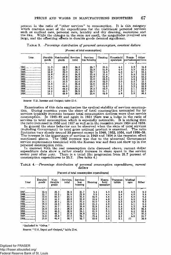
present in the ratio of “ other services” to consumption. It is this category which contains most of the expenditures for the traditional personal services such as medical care, personal care, laundry and dry cleaning, recreation and the like. While the changes in the ratio are small, the magnitudes involved are large, and the offsetting effects in durable goods demand significant.
T a b l e 3 .— Percentage distribution of personal consumption, constant dollars
PRICES AND WAGES IN MANUFACTURING INDUSTRIES 67
[Percent of total consumption]
Year Durablegoods
Nondurablegoods
Servicestotal
Services less housing
Housing Householdoperation
Transportation
Otherservices
1947....................... 11.9 53.8 34.3 23.7 10.5 4.4 3.9 15.31948....................... 12.3 52.7 34.9 23.9 1 1 .0 4.6 3.9 15.51949...................... 12.9 52.0 35.1 23.7 11.4 4.6 3.7 15.41950....................... 14.8 50.4 34.8 23.4 11.4 4.7 3.5 15.21951....................... 13.4 50.9 35.8 23.8 11.9 5.0 3.6 15.21952....................... 12.7 51.3 36.0 23.9 1 2 . 2 5.0 3.6 15.21953....................... 14.1 50.3 35.6 23.6 1 2 . 0 5.0 3.5 15.11954....................... 13.6 50.1 36.3 24.0 1 2 . 2 5.1 3.3 15.61955........ ............. 15.5 49.0 35.5 23.7 1 1 . 8 5.3 3.2 15.21956....................... 14.4 49.3 36.3 24.3 1 2 . 0 5.5 3.1 15.61957....................... 14.2 49.0 36.9 25.2 11.7 5.7 3.1 15.71958....................... 13.1 48.9 38.0 25.0 13.0 5.9 3.0 16.1
Source: U.S. Income and Output; table II-5.
Examination of this data emphasizes the cyclical stability of services consumption. During recession years the share of total consumption accounted for by services typically increases because total consumption declines more than service consumption. In 1948-49 and again in 1954 there was a bulge in the ratio of services to total consumption which is especially noticeable. It is striking that the ratio increased in 1956 and 1957 as well as in the recession years 1954 and 1958.
In general the same behavior can be observed when the ratio of total services (including Government) to total gross national product is examined. The ratio fluctuates very closely around 33 percent except in 1949, 1952, 1954, and 1956-58. The increase in the importance of services in 1949 and 1954 is the recession effect mentioned above. The 1952 increase was due to the abnormal Government service requirements associated with the Korean war and does not show up in the personal consumption ratio.
In contrast with the real consumption data discussed above, current dollar expenditure data show a rather steady increase in share spent in the service sector year after year. There is a trend like progression from 21.7 percent of consumption expenditures to 25.7. (See table 4.)
T a b l e 4.— Percentage distribution of personal consumption expenditures, currentdollars
[Percent of total consumption expenditures]
YearDurable
goodsNon
durablegoods
Services,total
Servicesless
housingHousing
Household
operation
Transportation
Medicalcare Other
1947............... 12.4 56.5 31.1 21.7 9.4 4.5 3.3 4.6 9.21948............... 12.7 55.3 31.9 2 2 . 0 9.9 4.4 3.4 4.9 9.41949............... 13.6 53.3 33.1 22.5 1 0 .6 4.6 3.4 5.0 9.51950............... 15.6 51.2 33.3 22.4 10.9 4.8 3.2 5.0 9.41951............... 14.1 50.1 33.5 22.5 1 1 .0 4.8 3.3 5.0 9.21952............... 13.2 52.4 34.4 22.9 11.5 4.9 3.4 5.1 9.51953............... 14.1 50.7 35.2 23.4 1 1 . 8 5.0 3.4 5.2 9.61954............... 13.6 50.1 36.3 24.1 1 2 .2 5.1 3.3 5.5 1 0 .11955............... 15.4 48.6 36.0 24.1 11.9 5.2 3.2 5.4 1 0 .11956............... 14.2 48.7 37.0 24.9 1 2 .1 5.5 3.2 5.7 10.51957............... 14.0 48.3 37.5 25.1 .12.4 5.5 3.1 5.8 10.71958............... 1 2 .8 48.4 38.7 25.7 13.0 5.8 3.1 0 ) 16.9
1 Included in “ Other.”Source: “ U.S. Input and Output,” table II-6.
Digitized for FRASER http://fraser.stlouisfed.org/ Federal Reserve Bank of St. Louis
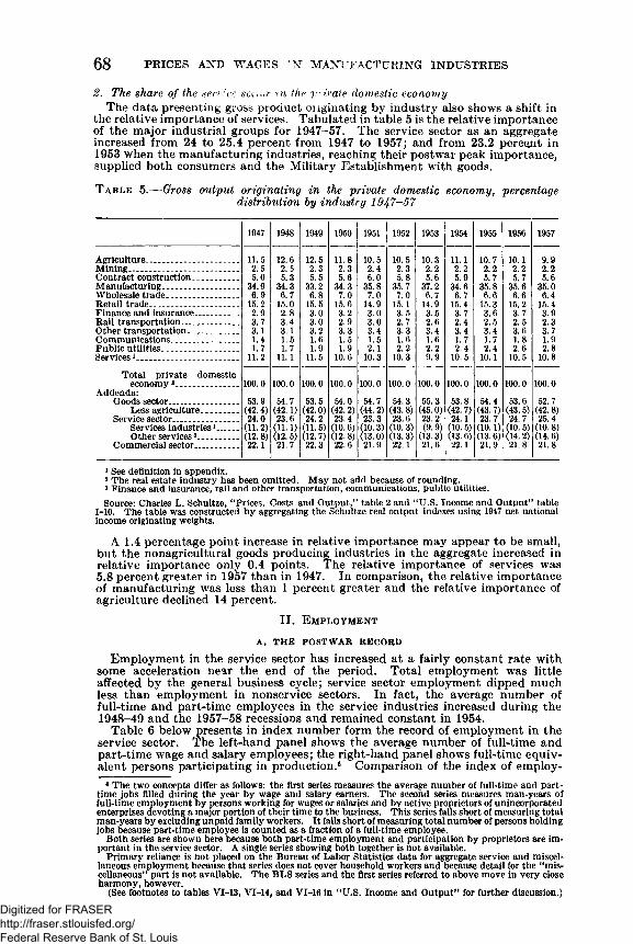
2. The share of the serricc sec, or m the ??*ivaie domestic economyThe data presenting gross product oiiginating by industry also shows a shift in
the relative importance of services. Tabulated in table 5 is the relative importance of the major industrial groups for 1947-57. The service sector as an aggregate increased from 24 to 25.4 percent from 1947 to 1957; and from 23.2 percent in 1953 when the manufacturing industries, reaching their postwar peak importance, supplied both consumers and the Military Establishment with goods.
6 8 PRICES AND WAGES TN MANT'FACTURING INDUSTRIES
T a b l e 5.— Gross output originating in the private domestic economy, percentage distribution by industry 1947-57
1947 1948 1949 1950 1951 1952 1953 1954 1955 1956 1957
Agriculture........................... ........... 11.5 1 2 .6 12.5 1 1 . 8 10.5 10.5 10.3 1 1 .1 10.7 1 0 .1 9.9Mining....... ................- .................... 2.5 2.5 2.3 2.3 2.4 2.3 2 . 2 2 . 2 2 . 2 2 . 2 2 . 2Contract construction____ ______ 5.0 5.3 5.5 5.6 6 . 0 5.8 5.6 5.9 5.7 5.7 5.6Manufacturing_________________ 34.9 34.3 33.2 34.3 35.8 35.7 37.2 34.6 35.8 35.6 35.0Wholesale trade____ ____________ 6.9 6.7 6 . 8 7.0 7.0 7.0 6.7 6.7 6 . 6 6 . 6 6.4Retail trade.................... ............... 15.2 15.0 15.5 15.6 14.9 15.1 14.9 15.4 15.3 15.2 15.4Finance and insurance__________ 2.9 2 . 8 3.0 3.2 3.0 3.5 3.5 3.7 3.6 3.7 3.9Rail transportation........................ 3.7 3.4 3.0 2.9 3.0 2.7 2 . 6 2.4 2.5 2.5 2.3Other transportation______ _____ 3.1 3.1 3.2 3.3 3.4 3.3 3.4 3.4 3.4 3.6 3.7Communications............. ........... 1.4 1.5 1 .6 1.5 1.5 1 . 6 1 . 6 1.7 1.7 1 . 8 1.9Public utilities............................... 1.7 1.7 1.9 1.9 2 .1 2 . 2 2 . 2 2.4 2.4 2 . 6 2 . 8Services1............... .......................... 1 1 . 2 1 1 .1 11.5 1 0 .6 10.3 10.3 9.9 10.5 1 0 .1 10.5 1 0 . 8
Total private domesticeconomy 2-------------- ------- 1 0 0 .0 1 0 0 .0 1 0 0 .0 1 0 0 .0 1 0 0 .0 1 0 0 .0 1 0 0 .0 1 0 0 .0 1 0 0 .0 1 0 0 .0 1 0 0 .0
Addenda:Goods sector__________ ____ 53.9 54.7 53.5 54.0 54.7 54.3 55.3 53.8 54.4 53.6 52.7
Less agriculture-.............. (42.4) (42.1) (42.0) (42.2) (44. 2) (43.8) (45.0) (42.7) (43.7) (43.5) (42.8)Service sector................ - _____ 24.0 23.6 24.2 23.4 23.3 23.6 23.2 24.1 23.7 24.7 25.4
Services industries1_____ (11 . 2 ) (11 . 1) (11.5) (1 0 . 6 ) (10.3) (10.3) (9.9) (10. 5) (1 0 . 1) (10.5) (1 0 . 8 )Other services3___......... (12 . 8 ) (12. 5) (12.7) (1 2 . 8 ) (13.0) (13.3) (13.3) (13.6) (13.6) (14.2) (14.6)
Commercial sector..... .......... 2 2 .1 21.7 22.3 2 2 . 6 21.9 2 2 . 1 2 1 . 6 2 2 .1 21.9 2 1 . 8 2 1 . 8
1 See definition in appendix.2 The real estate industry has been omitted. May not add because of rounding.3 Finance and insurance, rail and other transportation, communications, public utilities.
Source: Charles L. Schultze, “ Prices, Costs and Output,” table 2 and “ U.S. Income and Output” table 1-10. The table was constructed by aggregating the Schultze real output indexes using 1947 net national income originating weights.
A 1.4 percentage point increase in relative importance may appear to be small, but the nonagricultural goods producing industries in the aggregate increased in relative importance only 0.4 points. The relative importance of services was5.8 percent greater in 1957 than in 1947. In comparison, the relative importance of manufacturing was less than 1 percent greater and the relative importance of agriculture declined 14 percent.
II. E m p l o y m e n t
A . THE POSTWAR RECORD
Employment in the service sector has increased at a fairly constant rate with some acceleration near the end of the period. Total employment was little affected by the general business cycle; service sector employment dipped much less than employment in nonservice sectors. In fact, the average number of full-time and part-time employees in the service industries increased during the1948-49 and the 1957-58 recessions and remained constant in 1954.
Table 6 below presents in index number form the record of employment in the service sector. The left-hand panel shows the average number of full-time and part-time wage and salary employees; the right-hand panel show's full-time equivalent persons participating in production.6 Comparison of the index of employ-
• The two concepts differ as follows: the first series measures the average number of full-time and part- time jobs filled during the year by wage and salary earners. The second series measures man-years of full-time employment by persons working for wages or salaries and bv active proprietors of unincorporated enterprises devoting a major portion of their time to the business. This series falls short of measuring total man-years by excluding unpaid family workers. It falls short of measuring total number of persons holding jobs because part-time employee is counted as a fraction of a full-time employee.
Both series are shown here because both part-time employment and participation by proprietors are important in the service sector. A single series showing both together is not available.
Primary reliance is not placed on the Bureau of Labor Statistics data for aggregate service and miscellaneous employment because that series does not cover household workers and because detail for the “miscellaneous” part is not available. The BLS series and the first series referred to above move in very close harmony, however.
(See footnotes to tables VI-13, VI-14, and VI-16 in “ U.S. Income and Output” for further discussion.)
Digitized for FRASER http://fraser.stlouisfed.org/ Federal Reserve Bank of St. Louis
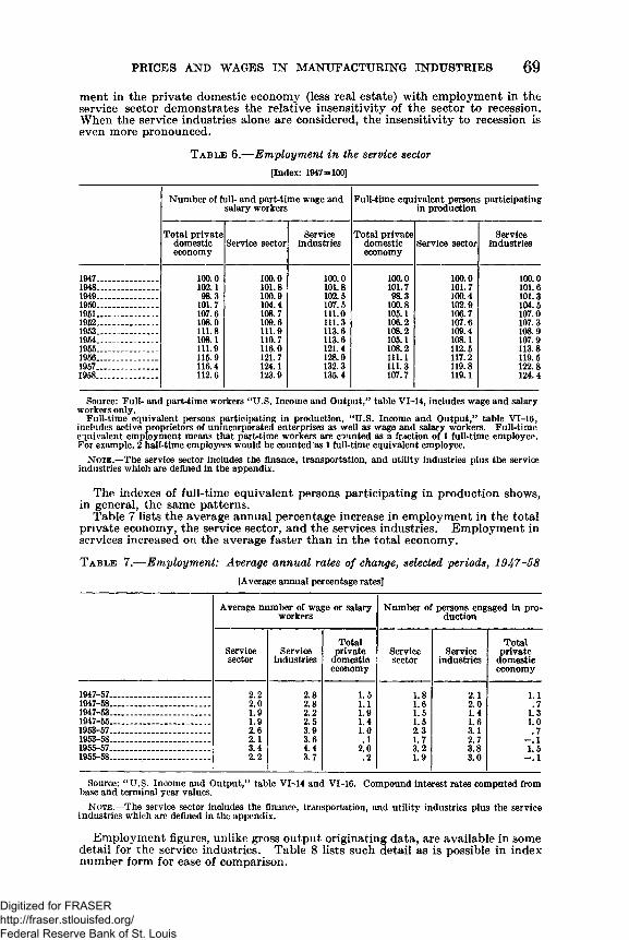
PRICES AND WAGES IN MANUFACTURING INDUSTRIES 69ment in the private domestic economy (less real estate) with employment in the service sector demonstrates the relative insensitivity of the sector to recession. When the service industries alone are considered, the insensitivity to recession is even more pronounced.
T a b l e 6 .— Employment in the service sector[Index: 1947=100]
Number of full- and part-time wage and salary workers
Full-time equivalent persons participating in production
Total private domestic economy
Service sectorService
industriesTotal private
domestic economy
Service sectorService
industries
1947........................ 1 0 0 .0 1 0 0 .0 1 0 0 .0 1 0 0 .0 1 0 0 .0 1 0 0 .01948......................... 1 0 2 .1 1 0 1 .8 1 0 1 .8 101.7 101.7 1 0 1 .61949......................... 98.3 100.9 102.5 98.3 100.4 101.31950.......................... 101.7 104.4 107.5 1 0 0 .8 102.9 104.51951....................— 107.6 108.7 1 1 1 .0 105.1 106.7 107.01952......................... 108.9 109.6 111.3 106.2 107.6 107.31953........................ 1 1 1 .8 111.9 113.6 108.2 109.4 108.91954_____________ 108.1 110.7 113.6 105.1 108.1 107.91955______________ 111.9 116.0 121.4 108.2 112.5 113.81956........... ............. 115.9 121.7 128.9 1 1 1 .1 117.2 119.51957........... ............. 116.4 124.1 132.3 111.3 119.8 1 2 2 .81958....... ................. 1 1 2 .6 123.9 135.4 107.7 119.1 124.4
Source: Full- and part-time workers “ U.S. Income and Output,” table VI-14, includes wage and salary workers only.
Full-time equivalent persons participating in production, “ U.S. Income and Output,” table VI-16, includes active proprietors of unincorporated enterprises as well as wage and salary workers. Full-time equivalent employment means that part-time workers are counted as a fraction of 1 full-time employee. For example, 2 half-time employees would be counted as 1 full-time equivalent employee.
N ote.— The service sector includes the finance, transportation, and utility industries plus the service industries which are defined in the appendix.
The indexes of full-time equivalent persons participating in production shows, in general, the same patterns.
Table 7 lists the average annual percentage increase in employment in the total private economy, the service sector, and the services industries. Employment in services increased on the average faster than in the total economy.
T a b l e 7.— Employment: Average annual rates of change, selected periods, 1947-58[Average annual percentage rates]
Average number of wage or salary workers
Number of persons engaged in production
Servicesector
Serviceindustries
Totalprivate
domesticeconomy
Servicesector
Serviceindustries
Totalprivate
domesticeconomy
1947-57.......................................... 2 . 2 2 . 8 1.5 1 . 8 2 . 1 1 . 11947-58....... .................................. 2 . 0 2 . 8 1 .1 1 .6 2 . 0 .71947-53.......................................... 1.9 2 . 2 1.9 1.5 1.4 1.31947-55.......................................... 1.9 2.5 1.4 1.5 1 . 6 1 . 01953-57......... ............................... 2 . 6 3.9 1 . 0 2.3 3.1 .71953-58.......................................... 2 . 1 3.6 . 1 1.7 2.7 - . 11955-57.......................................... 3.4 4.4 2 . 0 3.2 3.8 1.51955-58.......................................... 2 . 2 3.7 . 2 1.9 3.0 - . 1
Source: “ U.S. Income and Output,” table VI-14 and VI-16. Compound interest rates computed from base and terminal year values.
N ote.— The service sector includes the finance, transportation, and utility industries plus the service industries which are defined in the appendix.
Employment figures, unlike gross output originating data, are available in some detail for the service industries. Table 8 lists such detail as is possible in index number form for ease of comparison.
Digitized for FRASER http://fraser.stlouisfed.org/ Federal Reserve Bank of St. Louis
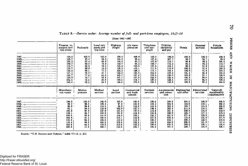
oT a b le 8.— Service sector: Average number of full- and part-time employees, 1947—58
[Base: 1947=100]
Finance, insurance and real estate
RailroadsLocal railroads and bus lines
Highwayfreight
Air transportation
Telephone and tele
graph
Utilities, electricity
and gasHotels
Personalservices
Privatehouseholds
1947....................................................... 1 0 0 .0 1 0 0 .0 1 0 0 .0 1 0 0 .0 1 0 0 .0 1 0 0 .0 1 0 0 .0 1 0 0 .0 1 0 0 .0 1 0 0 .01948................................ .................... 103.7 97.4 86.4 104.5 96.4 107.8 107.7 99.0 98.7 99.81949.................................... .................. 105.2 87.4 83.9 104.0 95.2 107.0 110.7 96.3 96.2 1 0 1 .61950.................................... .................. 109.7 89.0 79.3 113.7 95.2 103.7 1 1 2 .2 95.5 96.2 112.71951...................................................... 114.7 92.9 76.3 124.2 103.6 107.8 114.1 98.8 97.9 114.01952.......................................... .......... 118.7 89.6 73.2 128.2 118.1 1 1 1 .8 115.8 1 0 0 .8 97.8 108.21953.............. —..................... .............. 123.2 8 8 .1 71.2 134.2 126.5 115.7 118.1 102.9 97.4 109.51954.................................... ................. 127.5 78.2 67.7 132.2 126.5 114.8 119.2 101.4 96.4 105.01955..................................................... 133.7 77.6 62.6 140.7 137.4 116.6 1 2 0 .0 102.9 97.1 1 2 0 .81956.................................... ................. 139.3 76.7 58.6 147.7 157.9 123.6 122.4 105.3 98.8 129.41957.................................... .................. 142.5 72.4 56.6 149.5 174.7 130.0 123.4 107.0 98.8 129.21958...................................................... 145.4 62.2 53.5 144.8 173.5 1 2 0 .1 123.6 105.5 97.5 134.8
Miscellaneous repair
Motionpictures
Medicalservices
Legalservices
Commercial and trade
schools
Businessservices
Amusements and recrea
tion
Engineering and other
Educationalservices
Nonprofitmembership
organizations
1947..................................................... 1 0 0 .0 1 0 0 .0 1 0 0 .0 1 0 0 .0 1 0 0 .0 1 0 0 .0 1 0 0 .0 1 0 0 .0 1 0 0 .0 1 0 0 .01948.................................... .................. 96.4 98.4 106.4 97.4 1 1 0 .8 105.5 104.8 114.0 1 1 0 .1 1 0 2 .21949.................................... ................. 90.6 98.8 110.3 98.3 118.9 104.5 103.4 109.7 114.8 104.01950...................................................... 92.1 98.0 118.9 1 0 2 .6 127.0 108.4 102.4 1 1 1 .8 116.6 106.71951.................................... .................. 102.9 97.6 127.9 107.0 127.0 116.8 101.4 140.9 116.9 110.91952.................................... ............. — 1 1 0 .1 95.7 133.8 107.8 113.5 125.8 1 0 0 .0 166.7 117.5 113.41953.....................................................- 108.6 92.5 141.0 110.3 108.1 134.2 1 0 1 .0 177.4 1 2 0 .8 116.01954...................................................... 103.6 91.3 150.0 1 1 2 .1 1 1 0 .8 137.9 100.3 175.3 125.8 117.91955......................... ............................ 1 1 0 .8 90.5 158.6 112.9 116.2 149.2 103.1 193.5 132.6 119.41956.................................... ................. 119.4 8 8 . 6 169.3 113.8 132.4 165.5 104.8 236.6 141.8 127.41957............................................... ....... 125.9 84.2 178.5 113.8 143.2 180.0 105.5 249.5 150.1 133.61958......................... ........................ 1 2 0 .8 77.5 186.7 119.8 135.1 186.3 107.6 238.7 155.8 138.1
Source: “ U.S. Income and Output,” table VI-14, p. 212.
PRICES AND
WAG
ES IN
MA
NU
FAC
TUR
ING
IN
DU
STR
IES
Digitized for FRASER http://fraser.stlouisfed.org/ Federal Reserve Bank of St. Louis
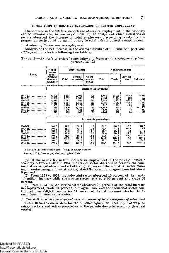
PRICES AND WAGES IN MANUFACTURING INDUSTRIES 71
B. THE SHIFT IN RELATIVE IMPORTANCE OF SERVICE EMPLOYMENT
The increase in the relative importance of service employment in the economy can be demonstrated in two ways: First by an analysis of which industries or sectors absorbed the increase in total employment; second by analyzing the proportion contributed by each industry to total private domestic employment.1. Analysis of the increase in employment
Analysis of the net increase in the average number of full-time and part-time employees indicates the following (see table 9):
Table 9.— Analysis^of sectoral contributions to increases in employment, selectedperiods 1947-58
Period
Net increase total
private domestic economy i
Service sector Nonservice sector
TotalService
industriesOther
servicesector
Total TradeAgricul
ture Industrial
Increase (in thousands)
1947-57................... 6,898 2,833 2,035 798 4,065 2,105 -359 2,3191947-58......................... 5,280 2,817 2,231 586 2,463 1,969 -308 8021947-53......................... 4,945 1,397 862 535 3,548 1,305 -325 2,5681947-55......................... 5,010 1,884 1,351 533 3,126 1,532 —363 1,9571953-57......................... 1,953 1,436 1,173 263 517 800 -3 4 -2491953-58........................ 335 1,420 1,369 51 -1,085 664 17 -1 , 7661955-57................... 1 ,8 8 8 949 684 265 939 573 4 3621955-58......................... 270 933 880 53 -663 437 55 -1,155
Increase (in percentage)
1947-57................... . . . 1 0 0 .0 41.1 29.5 1 1 . 6 58.9 30.5 -5 .2 33.61947-58......................... 1 0 0 .0 53.4 42.3 1 1 .1 46.6 37.3 -5 .8 15.21947-53........................ 1 0 0 .0 28.3 17.4 1 0 .8 71.7 26.4 - 6 . 6 51.91947-55.......... .......... 1 0 0 .0 37.6 27.0 1 0 . 6 62.4 30.6 -7 .2 39.11953-57......................... 1 0 0 .0 73.5 60.1 13.5 26.5 41.0 -1 .7 -1 2 .71953-58..-................... 1 0 0 .0 423.9 408.7 15.2 -323.9 198.2 5.1 -527.21955-57.............. .......... 1 0 0 .0 50.3 36.2 14.0 49.7 30.3 . 2 19.21955-58......................... 1 0 0 .0 345.5 325.9 19.6 -245.6 161.9 20.4 -427.8
i Full- and part-time employees. Wage or salary workers. Source: “ U.S. Income and Output,” table VI-14.
(a) Of the nearly 6.9 million increase in employment in the private domestic economy between 1947 and 1957, the service sector absorbed 41 percent, the commercial sector (wholesale and retail trade) 30 percent, the industrial sector (mining, manufacturing, and construction) about 34 percent and agriculture lost about 5 percent.
(b) From 1955 to 1957, the industrial sector absorbed 19 percent of the nearly1.9 million increase while the service sector took over 50 percent and trade 30 percent.
(c) From 1953-57, the service sector absorbed 73 percent of the total increase in employment, trade 41 percent; but agriculture and the industrial sector contributed over 280,000 persons (or 14 percent of the net increase) who had to be reemployed in some other sector.2. The shift to service employment as a proportion of total man-years of labor used
Table 10 makes use of data for the full-time equivalent labor input of wage or salary workers and active proprietors in the private domestic economy (less real estate).
Digitized for FRASER http://fraser.stlouisfed.org/ Federal Reserve Bank of St. Louis
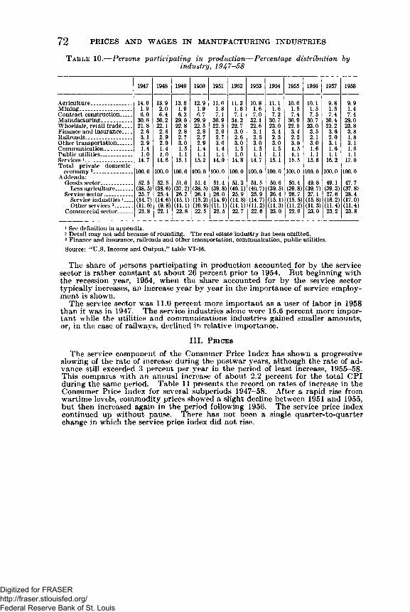
72 PRICES AND WAGES IN MANUFACTURING INDUSTRIES
T a b l e 10.— Persons participating in production— Percentage distribution byindustry, 1947-58
1947 1948 1949 1950 1951 1952 1953 1954 1955 1956 1957 1958
Agriculture______________ 14.0 13.9 13.8 12.9 11.6 11.2 10.8 11.1 10.6 10.1 9.8 9.9Mining----------------- ------- 1.9 2.0 1.9 1.9 1.8 1.8 1.6 1.6 1.5 1.5 1.5 1.4Contract construction 6.0 6.4 6.3 0.7 7.1 7.1 7.0 7.2 7.4 7.5 7.4 7.4Manufacturing---------------- 30.6 30.2 29.0 29.9 30.9 31.2 32.1 30.7 30.9 30.7 30.4 29.0Whoelsale, retail trade___ 21.8 22.1 22.8 22.5 22.5 22.7 22.6 23.0 22.9 23.0 23.2 23.8Finance and insurance___ 2.6 2.6 2.8 2.8 2.9 3.0 3.1 3.4 3.4 3.5 3.6 3.8Railroads____ ____________ 3.1 2.9 2.7 2.7 2.7 2.6 2.5 2.3 2.2 2.1 2.0 1.8Other transportation_____ 2.9 2.9 3.0 2.9 3.0 3.0 3.0 3.0 3.0 3.0 3.1 3.1Com in unication............. 1.4 1.4 1.5 1.4 1.4 1.5 1.5 1.5 1.5 1.6 1.6 1.6Public utilities....... .......... . 1.0 1.0 1.1 1.1 1.1 1.0 1.1 1.1 1.1 1.1 1.1 1.1Services 1_______ _________Total private domestic
14.7 14.6 15.1 15.2 14.9 14.8 14.7 15.1 15.5 15.8 16.2 17.0
economy 2................. .......Addenda:
1 0 0 .0 1 0 0 .0 1 0 0 .0 1 0 0 .0 1 0 0 .0 1 0 0 .0 1 0 0 .0 1 0 0 .0 1 0 0 .0 1 0 0 .0 1 0 0 .0 1 0 0 .0Goods sector______ _____ 52.5 52.5 51.0 51.4 51.4 51.3 51.5 50.6 50.4 49.8 49.1 47.7
Less agriculture........... (38.5) (38.6) (37.2) (38.5) (39.8) (40.1) (40. 7) (39. 5) (39.8) (39. 7) (39.3) (37. 8)Service sector.................. 25.7 25.4 26.2 26.1 26.0 25.9 25.9 26.4 26.7 27.1 27.6 28.4
Service industries 1___ (14.7) (14.6) (15.1) (15.2) (14.9) (14.8) (14. 7) (15.1) (15. 5) (15.8) (16.2) (17.0)Other services3......... (11 . 0 ) (9.8) (11 . 1) (10.9) (It.1) (1 1 . 1) (1 1 . 2 ) (11.3) (1 1 . 2 ) (11.3) (11.4) (11.4)
Commercial sector_____ 2 1 . 8 2 2 . 1 2 2 . 8 22.5 22.5 22.7 2 2 . 6 23.0 22.9 23.0 23.2 23.8
1 See definition in appendix.2 Detail may not add because of rounding. The real estate industry has been omitted.3 Finance and insurance, railroads and other transportation, communication, public utilities.Source: “ U.S. Income and Output," table VI-16.
The share of persons participating in production accounted for by the service sector is rather constant at about 26 percent prior to 1954. But beginning with the recession year, 1954, when the share accounted for by the seivice sector typically increases, an increase year by year in the importance of service employment is shown.
The service sector was 11.0 percent more important as a user of labor in 1958 than it was in 1947. The service industries alone were 15.6 percent more important while the utilities and communications industries gained smaller amounts, or, in the case of railways, declined in relative importance.
III. P r ic e s
The service component of the Consumer Price Index has shown a progressive slowing of the rate of increase during the postwar years, although the rate of advance still exceeded 3 percent per year in the period of least increase, 1955-58. This compares with an annual increase of about 2.2 percent for the total CPI during the same period. Table 11 presents the record on rates of increase in the Consumer Price Index for several subperiods 1947-58. After a rapid rise from wartime levels, commodity prices showed a slight decline between 1951 and 1955, but then increased again in the period following 1956. The service price index continued up without pause. There has not been a single quarter-to-quarter change in which the service price index did not rise.
Digitized for FRASER http://fraser.stlouisfed.org/ Federal Reserve Bank of St. Louis
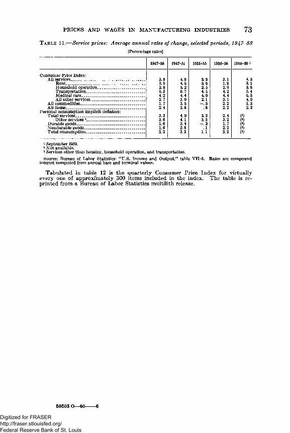
PRICES AND WAGES IN MANUFACTURING INDUSTRIES 73T a b l e 11.— Service prices: Average annual rates of change, selected periods, 1947-58
[Percentage rates]
1947-58 1947-51 1951-55 1955-58 1955-59 i
Consumer Price Index:All services. __ ______________________________ 3.8 4.8 3.3 3.1 4.3
Rent.......... ................................. .............. ............ 3.5 4.6 3.6 1.9 3.1Household operation_______________________ 2.8 3.2 2.5 2.9 3.8Transportation_____________________________ 6.3 9.7 4.5 4.2 5.4Medical care_______________________________ 4.2 4.4 4.0 4.4 6.3All other services___________________________ 2.7 3.0 2.1 3.1 4.0
All commodities________________________________ 1.7 3.5 - . 3 2.2 1.3All items_______________________________________ 2.4 3.8 .8 2.2 2.3
Personal consumption implicit deflators:Total services....................... ...................................... 3.3 4.0 3.2 2.4 (2)
(2)(2)(*)(2)
Other services 3_____________________________ 3.6 4.1 3.3 3.2Durable goods.___ ______ __ ______________ 1.6 3.4 - . 2 1.7Nondurable goods______________________________ 1.6 2.8 . 1 2 . 2Total consumption_____________________________ 2 . 2 3.2 1 .1 2 . 2
1 September 1959.2 Not available.3 Services other than housing, household operation, and transportation.Source: Bureau of Labor Statistics: “ U.S. Income and Output,” table VTI-3. Rates are compound
interest computed from annual base and terminal values.
Tabulated in table 12 is the quarterly Consumer Price Index for virtually every one of approximately 300 items included in the index. The table is reprinted from a Bureau of Labor Statistics multilith release.
50505 0 — 60--------6
Digitized for FRASER http://fraser.stlouisfed.org/ Federal Reserve Bank of St. Louis
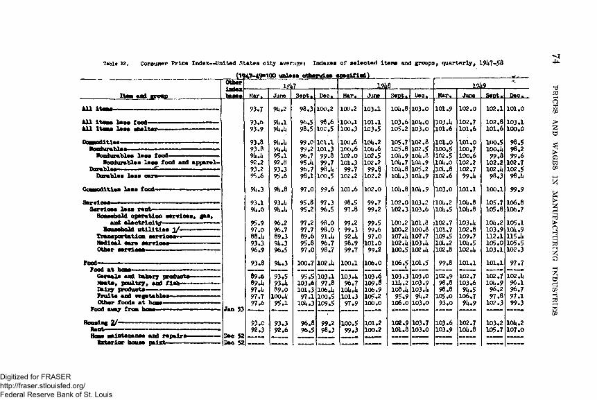
Table 12. Consumer Price Index— United States city •vernier Indexes of selected items and groups, quarterly, 19147-58 2
It— and group
A l l it« M -
A l l lt« M leas food— ▲11 items less ahelte
R o o to tb lN less food-Noadurtbks less food and apparel-
Durab leaDurables leas oara-
C aa o d itia a leas food-
3arrloee-Serrloaa lass re n t-
Houaehol d operation aerrioea, and a la o tr lo lty - ■■■ — ■—
Household u t i l i t ie e j / — Tranapartation eerrioea— M rtloa l oare aervioaa— — ~ Other aarriooa- ■ -
*•»
Food-Food a t horns
Caraala and bakery Msata, poultry, and f i s Daiiy produota— — — Fru ita and vegatablta- Othar fooda a t h e n
Food awaj tram hcai
Housing 2/-Rant-Hcne Maintenance and repalre
Exterior house paint—
( ly H ^ I Q O unleaa otherwise
ou* pl I'Mindex-------baaas Mar,
53
June
9U.2
9U.19U.U9U.U y U.h95.1 92.893.395.6
9U.8
93.U9U.U
96.296.789.3 9lw396.5
9U.3
93.5 93.U89.0
100.1495.1
93.392.6
Sefit*.98.3
96.598.5
99.0 9V.296.7 95 .U96.798.1
97.0
95.895.2
97.297.789.695.897.0
100.7
96.896.5
Dec.
100.298.6
IOC.5101.1 101.3 99.8 99.7 98.14
100.5
99.6
97.396.5
98.098.0 91.U96.798.7
102.ii103.1
97.8 106.li100.5109.5
99.298.3
Md t W )
Har.
100.2100.1100.3
100.6100.6102.0101.3
99.7 102.2101.6
98.597.8
99.299.3 92.1*98.9 99.7
100.1
June103.1
101.1103.5
10U.210U.6102.5 102.2
99.8102.2102.099.799.2
99.599.6 97.0
101.099.2
106.0
103.6 109 106.9 105.2 100.0
S*£tjIQI4.8
103.6105.2
105.71C5.81014.910U.710li.81014.3
IOI4.8
102.0102.3
100.2100.2107 .14 102.14100.5
106.5 »103.3 n i l . 2108 .14 95.9
106.0
102.9101.8
Dec.103.0
10 14 .0103.0
102.8102.51014 .8 10U9 105.2 101*.9106.9
103.2103.6
101.8 100.8 107.7 103 .14 10 2 .14
101.5
103.0103.9 103.14914.2
103.0
103.7103.0
Mar*.101.9
103. 14 101.6101.0100.5102.51014.0 101.8102.6103.0
10U.210U.5
102.7101.7 109.5 IOI4.2102.8
99.8
102.998.8 98.8
105.093.0
103.6103.9
J.21&
102.0102.7 101.6101.0100.7 100.6 102.2102.7 99.14
101.1lQii.8 10b. 8
103.14102.8 109.7 1014.510 2 .I4
101.1
102.710U.8
-Sgpli102.1102.8101.6
100.5 100.14
99.8 102.2 102 .I4
98.3
100.1
105.7105.8
1014.2103.9 112.1 105.0103.1
101.1
103.2105.7
101.0103.1 100.0
98.598.299.6
102.7102.5 96.14
99.9
106.8 106.7
105.1 10U.9 115.14105.5 102.3
97.7
102.1*96.196.797.199.3
10U.2107.0
PRICES AND
WAGES
IN M
ANUFACTURING IN
DU
STRIES
Digitized for FRASER http://fraser.stlouisfed.org/ Federal Reserve Bank of St. Louis
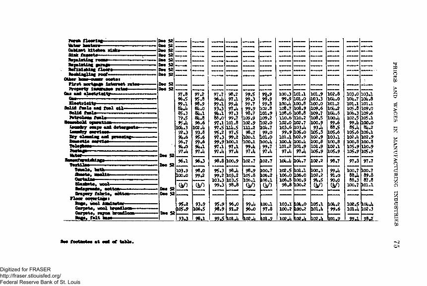
Ifetor h u t iw Cmbiaftt kltotett aix^» Sink fu p o ttt
Reahlegllag root' Otter
n p i w oi aadafUr G ir p it i i n o d 1
ngroa Hop, f o l t bu » 93*3
8m fookaoUa at Md of ttbla.
II
!!!!
Mi
ll
!ii
iiii
Hi
m -------- ----
----
Ni
l!! ---- ----
97.796.lt99.1 93.3 9lul 88.097.1 97.595.297.3 99.9 97.1 97.lt
98.297.1 99 J* 97 .U 97.3 99.7
101.811U.597.599.2 100.197A 97.U
99.599.399.7 99.998.7
109.9102.9 111.298.7
100.1 100.199.1*97.lt
9$.999.999.3
102.8101.9109.2102.010li.799.0
101.0100.lt99.797.lt
100.399.9
100.lt 108.7 108.6 110.6 102.0 103.699.9
101.1 100.lt 101.297.lt
101.1101.0100.8108.9 108.8 110.2 102.7 103.U 105.0102.9 100.lt101.9 974
101.9103.3 100.0109.6109.7 108.5100.9 93Jt
105.3102.9100.8101.9105.9
102.810U.0101.210lt.210lt.8100.lt99.688.5
105.6103.1 100.8102.1 105.9
103.010U.7101.1105.8106.3102.5 99.lt 85.lt105.6
102. it 100.8105.9105.9
103.110U.8101.1109.0 109.6105.1 100.08U.2
106.1102.9 100.3110.9105.9
98.8 100.9 102.7 102.7 10lt.lt 10lt.7 102.2 98.7 97.3 *7.795.399.2
103.399.3
~98ji103.2103.598.8
98.9105.8106.1(J*/)
L00.7L06.2L06.1(h/)
102.5106.0106.398.8
101.1106.0100.9100.2
100.3102.29it.5(1*0
99491.090.0(V)
100.7 88 J* 88.3
100.7
100.789.887.8101.1
95.996.9
96.091.2
99.U96.0
L00.197.8
103.1100.2 10U.0100.2 105.110l.lt
10U.299.6
102.5lOIJi
ioit.lt102.3
?9.S I01.lt 102 .1* L01.9 102.1*tl02.il 11024 tioi*? 99.1 98.2
Oi
PRICES AND
WAGES
IN M
ANUFACTURING IN
DU
STRIES
Digitized for FRASER http://fraser.stlouisfed.org/ Federal Reserve Bank of St. Louis
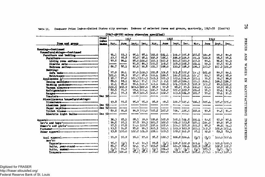
Table 12. Consumer Price lnd*x— United States city average: Indexes of selected items and groups, quarterly, 19li7«58 (Cont'd)
(1947-49=100 unless otherwise specified )________________
O i
Itia tad groupHousing— Continued
Housefurni ahinga— Continued Furniture and bedding—
Furniture-Living roon suite s - Dinette sets----- ----Bedrooa suites-
BeddingsSofa bede— —Mattressee-
Applianoes 2/~Sewing Machines---------Washing Machines———Vacuum cleaners---------Refrigerators-------- —Ranges----------------------Toasters-
Miscellanaous housefurnishings « Dinnerware— - ———----— - —
Otherindex
De c 52
Minima pans- Paper napkin Toilet tissue— - Electric light
Apparel——— lien's and boys' Vonen's and girls' Footwear-Other apparel----- —----
Wool apparel------------Men's*
Topcoats-Suits, year-round----- ----------Suits, sunraer————— -----Trousers-
DecDecDec 52
97*9101.195.786.591.1
1C1.589.596.1
93.8
89T6
96.396.697.593.593.8
91.9
95.788.7(W)ictf.o
JtijL
June Sept. Dec. Mar. June Sept. Dec.
93.3 95.14 98.1* 102.0 lo i .h 106.0 105.992.8 95.2 98.1; 102.2 105.1 106.9 106.696.li 98.0 100.C 102.3 102.2 103.5 103.9
91.6 96.3 101.5 106.5 109.C 108.78e.i 92.6 96.e 101.7 108.0 110.2 108.9
96.1; 97.6 100.3 101.8 101.6 ic i .e 102.298.3 98 .C 9 8 .6 101 J* 100.6 100.6 101 .If97.0 101.3 103.3 103.3 101.3 103.1 101.689.1 92.6 9^.5 99.7 1,2.1 105.0 106.195.0 99.1 101.7 1C2.1 100.9 10U.3 105.5
102.9 103.6 10C.0 98.9 97.8 98.2 99.691.7 99.1 lC l.ii 102.7 101.2 107.0 109.797.3 98.5 101.5 102.6 102.7 103.6 10U9
93.6 95.9 11 95.9 98.9 99.8 !1 100.7
0 1
• •
u\ 1
0 1
l-l 1
1 1
S I S
96.9 103.0 107.2 107.2 106."1------(105.5
97.1 98.1 99.9 102.6 102.9 ' 105.1
|
il0U.897.1 97.8 |5 99.3 101.7 102.5 ! ‘1014.2 103.897.8 99.ii i100.6 j102.6 102.6 j 106.1 105.99U.8 95.0,i 98.3 1103.3 103.1 II 103.9 103.9
100.0 102.2 1;1CU.9 109.6 1109.5|
! 109.0 105.9
92.9 96.6 | 97.0 96.e j100.3 | io6.e 106.1*
(V ) 9 ;.0{ 99.3 99.8 (V ) 102.7 102.990.5 92.1.! 95.7 1 0 3 . e ldT.e ;I 106.9 106. k91.7
100.0 WM(V )92.7 W l:
ioli.3 ! 1101.0 1
! (V )| 103.6
«/>licTI.o
191x8
Mar. June
il03.8 101.1 102.1 lCli.1* 106.3
l a .3lor .e 1 0 1 . 1 IC6 . 11 0 2 .9100.010it.2101.6
19L9
100.9100.6
99.199.3
103.0
101.099.7 96.6
106.1 1101.2
9* .6 i 9C.3 i 99 .c
102.6 j 99.e
101.1*1 0 1 . 11 0 1 . 2 1 0 3 . 1
9 7 . 1
(U/)i c i .14105.9(£/)
105.0.
I 9 .5 I100.0
98.21C2.7
I 92.0
( i /)a / )
105.C 1 0 5 . 3 11 -3.6
Sept. Dec
99.29 8 .e96.697.6
1C2.2
99.998.6 96.7
1 0 6 . 199.193.9 99.1; 90.JU
99.098.6 96.397.6
101.9
99.1 98.996.6
106.7 101.098.5 97. U95.5
105.0 105.0
9*.5 9U.9
97,99.96,
101,89,
>9 97.1 .0 98.9 ,0 9k .3 ,6 ilC l.ii ►3 89.3
103.5 jlC2.li
101.1 |l02.3102.6 jl02.7
(V ) 1 tt/) 10U.3 1 0 0 .3
PRICES AND
WAGES
IN M
ANUFACTURING IN
DU
STRIES
Digitized for FRASER http://fraser.stlouisfed.org/ Federal Reserve Bank of St. Louis
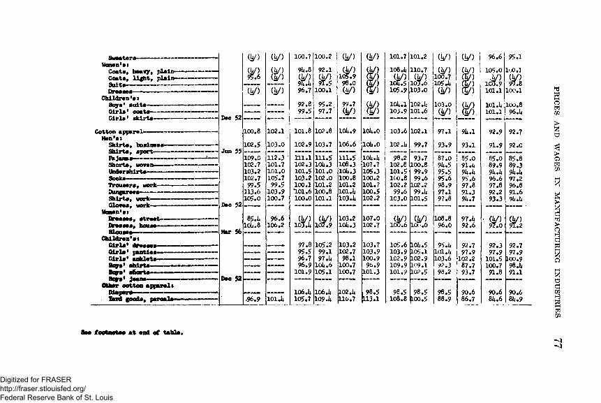
SweateWomen*®i
Coats, heavy, plain* Coats, ligh t, plain-Suits-----------------------Dresses—----------------
Children's!Boys' suits— ———G irls ' coats-----G irls ' skirts*
Cotton apparel - —— Men'st
Shirts* business Shirts, sport- FajanaiShorts, wovexv- UWershirts—— Socks-Trousers, work- DungaShirts, work- Gloves, work
women's!Dresses, street— Dresses,Blouses-
Children's t G irls ' dresses- G irls ' panties G irls ' a ilk le t s -
shirts—Beys' s&orts-
jeane-01 her ootton apparels
Diapalaid goods, peroale-
(U/) (h/)
(V )95.6
(V )< !/)
T kJ) Th/)
Dec 52 — —-------
100.8 102.1
Jun 55
Dee 52
102.5
109.0102.7 103*2102.7 99.5
113.6 105.0
103.0
112.3101.7 101.0105.7 99.5
103.9100.7
Mar 56
65.ii10li.8
W
i I
»'O
O 1
II*S
I i
1
Dee 52
-------
-------
.96.9 101 J*
8m footnotes at end of table*
100.7 100.2 (V ) (h/)
9U.8(V )95.ii96.7
92.1
■ as 100.1
(V )105.998.0(5 /) 1
92. e 99.5
95.2.97.7
99.7(V )
W )( y )
101.8 102.8 10U9 lou.o
102.9 103.7 106.6 lOli.O
111.1102.3101.5 103.2 100.1101.6 100.0
111.510U.3101.0102.0101.2100.8101.1
111.5108.3lQii.3100.8101.2101.li103.li
10li.ii107.7 105.3 100.2101.7 100.5 102.2
m (£ /)102.9
103.2 10li.3
107.0102.7
97.8 95.5 96.796.9
101.9
105.299.197.1*
10li.6105.1
103.2102.7
98.1100.7100.7
103.7103.9100.9 96.9
101.3
106.ii105i7
106.iiI09.ii
102 .li 116.7
98.5113.1
101.7 101.2 (y ) j (V )
108.14 110.7 (h/) I (V )(V )
iofi.5(V )
103.6100.7I05.il
& )W )
105.9 103.0 (h/) <S/>
lOlul 102.1- 103.0 U/>103.9 101.6
1 • IS
<5/)
103.6 102.1 97.1 9U.1
102.ii 99.7 93.9 93.1
98.2 93.7 87.0 85I0102.e loo.e 9U.5 91.5101.5 99.9 95.5 91i.lilo o .e 99.6 95.6 95.6102.2 102.2 98.9 97.899.6 99 .li 97.1 91.3
103.0 101.5 97.8 9li.7
(V )100.6(h/)
10O.0108.8
96.097 .5 92.6
105.6 10li.5 95.li 92.7103.9 105.1 lOl.ii 97.9102.9 102.9 103.6 102.2109.9 109.1 9?.3 87.7101.9 10? . 5 | 98.2 93.7
98.5 98.5 98.5 90.6108.8 L00.5 88.9 86.7
96.6 95.1
105.0 luO.l(V )97.8
101.1 100.1
101.li 100.8101.1 96.li
92.9 92.7
91.9 92 .0
*85.0 I 5I889.9 89.39li.li 9ii.ii96.6 97.297.8 96.892.2 91.693.3 91i.li
. <V) 92.0
(U/)91.2
92.3 92.797.9 97.9
101.5 100.9100.7 98.1|91.8 91.1
90.6 90.681u6 8Iu 9
•<1
PRICES AND
WAGES
IN M
ANUFACTURING IN
DU
STRIES
Digitized for FRASER http://fraser.stlouisfed.org/ Federal Reserve Bank of St. Louis
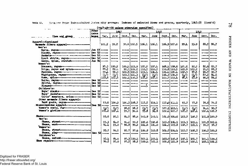
Table 12. Ccr.sj~»>r Price Indox— United Jtates city averages Indexes of selected items and groups, quarterly, 19U7-58 (Cont’d)
___ ___ ____Item and p oop
Apparel—ContinuedMamade fibers apparel— ■■
Men'ssSuite, rayon— — -------Slades, rayon---- — —Jacket®-— - — ----------- —Sport shirts, rayon-Socks, nylon, stretch--------- —
Woneo'stDresses, rayon— — ---------------Slips, rayon and nylon— —---------Panties, rayon- Nightgowns, rayon- Hoee, nylon— —Suits, rayon---- -----Skirts, rayon------—Blousea-----------------
Children's*Boys' slacks- Boys' jackets*G irls ' sweaters, orIon—
Other aaaade fibers apparel t lard goods, rayo
.Miscellaneous apparel- Vonen's ooats, fur—Woaen's girdles--------
Shoes-Han'si
Shoes, s treet- Shoes, work—
Vonsn'stShoes, s treet- Shoes, play— -
Children's t Shoes, oxford-
Shoe repairs——•—
Otherindexbases
(1947-4^100 unless otherwise specified)
JunDeeDeeDecJun
DeeDeeDec
DeoDeoDec
Dee 52
Dec 52
19b7 191*8 191*9Mar. June Sent. Dec. Mar. June Sept. Dec. Mar. June Seot. Dec.
i101.5 99.8 99.6 102.5 106.1 106.1 106.9 107.0 99 .U 93.9 88.2 86.7
I |
I T
^.-
iC00.
1 !
1 !
! :
SS
R3
IS
! !
!I
ll
H
il
l
100.2 89 J* 99.0 (h/)
102.3
100 J* 92.1
100.5 103.1 100.1*
103.9101.2100.5101.3100.7
107.2110.7103.1*
(V )102.2
•
107 .li 110.7 101* .1* (U/)
102.0
108.1*110.8106.1*106.3103.7
109.6 110.5 105.1* 106.9 103 .U
101.2.105.9102.0
(V )96.5
92.2103.297.5(y>93.9
85.691*?90.787.290.0
82.788.790.7 81* .6 89.5
93.0 100.3 105.3 108.7 117.5 119.1 117*0 l lu . l 93.2 73.2 76.5 76.5
l I/ >101.2
7u / )107.1*
~98l599.7
98.296.6 97.8 9u.8
107.1102.1*
103.U101.7
T h i)101.7
" (V )102.1*
91*.U102.1*
90.7102.7
93.6 95.1 91*.2 98.6 103.9 103 J* 101* .0 101**0 103.2 102.7 101.0 100.9
93.3 91*. 1*
91* .2 93.0
9l*.2 % 96.3
99.299.2
102.610l*.6
102.6 10k .0
103.9 101* .3
10l*.l103.8
103.3102.7
103.1*101.1
101.8 • 99.7
102.1*98.7
93.7 96.5 92.7 97.U 10U.9 103.8 101*.5 101*.1* 103.7 lOfc.S 100.2 100.2
93.1*96.5
9l*.697.0
97.397.2
100.1*98.2
103.U100.1*
103 .U 101.1•
103.0101.5
102.9101.9
102.1101.9
101.7102.1
101.1102.1
100.5101.5
00
PRICES AND
WAG
ES IN
MA
NU
FAC
TUR
ING
IN
DU
STR
IES
Digitized for FRASER http://fraser.stlouisfed.org/ Federal Reserve Bank of St. Louis
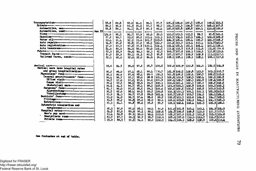
Transportation* Privata-
Autowobilaa, na v ■■ ■ Autonobilaa, uaad— - Tiraa-Gaaolina-Motor o i l - Auto rapairs-Auto ragiatration— Auto insuranoa——
Public------------------------Tranalt faiaa-——-------Railroad faraa, coach-
Jan 53
Madical cAre— — — — — — — —Madioal oara la a a hoapital rataa
and group hospitalitatio ftyalolana1 faas-
Ganaral practitioners1 Qtfioa v is it—— —
faaa-
Houaa r ia it -Obatatrioal oara-
Surgaona1 faas-Appendaotany— Tonaillaetosy
Dantlata*FillingsExtractiona-
Optonatrio axaalnation and ayaglaaaaa— — —
Hospital rataaHan's pay uard— Saniprivata rooa- Frivata roo»—
88.8 89.889.2 90.288.8 89.1
ioa.6 96.387.2 90.290.U 91 .U9U.8 95.297.9 97.98U.0 85.087.9 88.988.2 88.985.1 92.0
93.6 9U.7
95.2 96.096.1 96.696.U 96.796.5 97.097.2 97.293.6 9U.59U.7 96.095.5 97.693.9 9U.393.9 9lw993.8 95.293.3 9U.1
95.3 95.68lu5 87.683.U 86.883.7 87.785.9 88.5
Saa footnotas at and of tabla.
92.0 93.3 9U.1
9U.793.592.$95.897.9 86*089.089.1 92.0
96.097 .h97.697.797.298.596.797.598 .U96.796.796.896.8
97.089.988.2 90.391.5
97.2
98.198.198.0 97.1* 98.698.198.599.2 97.8 97 .U97.098.698.192.1 90.0 92.7 9U.1
98.8
99.199.0 98.8 9«.299.599.299.399.599.0 98.298.0 98.8
99 .k99.1 99.1* 98.799.2
100.5
1D0.7101.3101.3 101.9 100.1 102.8 101.0 100.8 101.U
99.599.699.7
99.9102.6103.0102.0 102.5
105.310U.7105.9
103.2 103.5 lOtu?103.2 101.U 112 .U 106.7 107.3 108.1
102.0101.9101.8101.6102.1100.6103.0102.5 102.3102.5 102.2 102 .U102.1101.0lOluS105.2105.0iou.5
106.0105.3105.8
102.9*
102.5 102.2 102.2102.7 101.1103.3102.5102.3102.5103.3103.8 102 .U101.8106.8107.2107.0106.3
107.5106.8108.8
103.8
102.8 102 .U102.3102.3102.3 102.8102.5 101.1103.7103.6 lO h .l 102 .U
103.li109.8 111.5 110.0 108.2
108.0107.5109.1
lOfc.O
103.2102.5 102 .14 101.8102.7 103.0102.8 101.1 10U.5 10U.5 10U.3 105.3
103 .U 110.2111.5110.7108.8
109.U108.0110.0
95.8106.3105.7103.7 loi.U 11U.6112.8113.1108.1
10U.5
103.3102.5102.5 102.1* 102.2103.3 103.0 101.9 1QU.1 10U.7 10U.3 105.9
1011.0111.3113.0 111.7109.6
110.3107.8109.9
10U.9
103.7 103.0102.8 102.8102.5103.3 103.8103.5 10U.1 105*5105.3 106.1
10U.0112.1llli.0112.0llO ji
o
PRICES AND
WAGES
IN M
ANUFACTURING IN
DU
STRIES
Digitized for FRASER http://fraser.stlouisfed.org/ Federal Reserve Bank of St. Louis
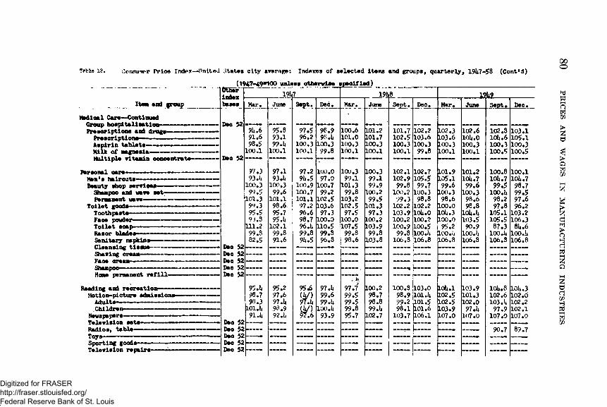
Table 12. Ccnsniirr Prioe Index— United States city average: Indexes of selected items and groups, quarterly, 191*7-58 (Cont*d)(1947-49*100 unless otherwise specified)
1917_________ 1 _______191*8_______________________ 19ii9
00o
Item and group
Msdloal Care— Continued Group hoepi tali sat ion~Prescriptions and drugs- Prescriptions- Aspirin tablets-Milk of Magnesia— —Multiple vitamin oonoentrate—
ftrsonal oare-Msn's haireuts-Beeuty shop services— Shampoo and wave eet- Fsrmanent '
Toilet goods-Toothpeste-Faoe powder- Toilet soap—Rasor blades-Sanitary napkins* Cleansing tissue- Shaving cream— Faoe oream— — —Shampoo.... ........Home permanent ref i 11-
Reading and recreation-Motion-picture admissions— Adults------------------Children-
Newspapers-Television sets- Radios, table— Toys— - — — — — Sporting goods Television repairs-
Otherindexbases
Deo 52
Deo 52
Deo 52 Deo 52 Deo 52 Dee 52 Deo 52
Deo 52 Deo 52 Deo 52 Dec 52 Deo 52
Mar*
9*4.691.698.5
100.1
97.3 93 .U100.3 99.$101.399.395.5 9J.3
111.299.382.5
95 .h 98.7 98.3
101 .U 91.U
June
95.8 93.1 99 .U
100.1
97.193.U100.399.6
101.198.695.7 95 .U
102.199.8 91*6
95.2 97.6 97 .U .98.9 92.h
Sept.
97.596.2100.3100.1
97.2 914.5100.9100.7101.197.296.698.7 96.U99.8 9U.5
95 «6( y )97.Um
Dec.
98.99?>.U100.399.8
100 .0 97.0
100.799.2102.5103.697.3
100.0 110.599.896.8
97.1499.699.U
100.1493.9
Mar.
100.6101.0100.3100.1
100.3 99.1101.399.8 103.2102.597.5
100.0107.599.898.6
97.799.599.599.8 95.7
Juno
101.2101.7100.3100.1
100.3 99.1 99.9
100.299.5101.3 97.3
100.2103.999.8103.8
LOO .298.798.8 99.U102.7
Sept. Dec.
101.7102.5100.3100.1
102.1102.999.8
100.299.3
102.2103.9 100.2100.999.8 106.3
100.398.999.298.1103.7
102.7105.599.7
100.398.8
102.2 IOI4.O 100.2100.5 IOOJ4106.8
103.0IOIJ4101.5101.6 106.1
Mar.
102.3 103.6100.3 100.1
101.9105.199.6 tL00.398.6
100.0 1014.3100.0 95.2
loo.;* 106.8
LOU.I102.5102.5 103.9 107.0
June
102.6IOI4.O100.3100.1
101.21014.799.6 100.398.69e.8
IOI4 J4
103.590.9
100.U106.8
103.9 101.3 102.0 97 .14 107.0
Sept.
102.81014.6100.3100.5
100.8IOI4.799.5
lOO.U98.297.8
105.1105.587.3IOO.I4106.3
1014.3 102.6 103 .U 97.9
107.090.7
Dec.
103.1105.1 100.3 100.5
100.1IOI4.798.799.597.6 96.2
103.2106.3 8U.6
100.14106.8
1014.3102.0102.2102.1107.0
89.7
PRICES AND
WAGES
IN M
ANUFACTURING
IND
USTRIES
Digitized for FRASER http://fraser.stlouisfed.org/ Federal Reserve Bank of St. Louis
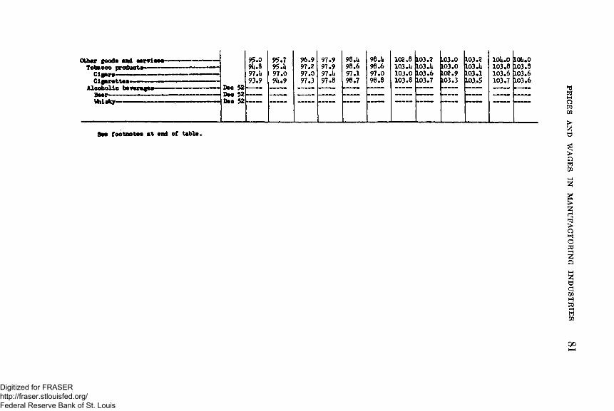
Other goods cod serrioee- Tobeooo produ
Cigars-Cigarettes—
Aleobollo b u t n g M - Beer- —Whisky-
Dee 52 Deo 52 Deo 52
95.09U.897.1*93.9
95.7 95.1* 97.0 9U.9 97.3 97.8
9*o footnotes st end of table.
98.1* 98.1* 102.8 103.2 103.0 103.2 lOluO XOtuO98.6 98.6 103.1* 103.1* L03.0 103.1* 103.8 [103.397.1 97.0 103.0 103.6 LOS .9 103.1 103.6 103.698.7 98.8 103.8 103.7 L03.3 103.5 103.7 103.6
---- ---- ---- ---- ---- ---- ---- ----
PRICES AND
WAGES
IN M
ANUFACTURING IN
DU
STRIES
Digitized for FRASER http://fraser.stlouisfed.org/ Federal Reserve Bank of St. Louis
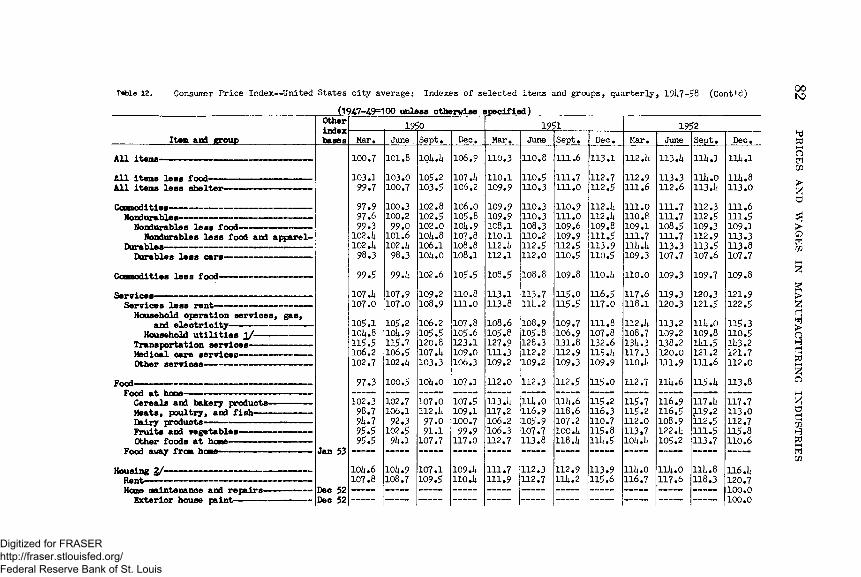
Consular Price Index—United States city average: Indexes o f selected items and groups, quarterly, 191*7-58 (Cont’ d)
(1947-49=100 u n le s s o th e rw ise s p e c i f ie d )__________________
00t o
Item and groupOtherindexbases Mar.
1950June S e p t. Dec. Mar.
1951June S e p t. D ec. Mar.
1952
June S e p t. D ec.
All items-All items less food-All items less shelter-Commodities- Nondurable s-Nondurables less food-Nondurables less food and apparel-
Durables— — — ----------------------Durables less cars-
Commodities less food-Services-Services less rent-Household operation services, gas,
and electricity— — --------- -Household utilities ±/~
Transportation services- Medical care serviceo- Other services-------
Food-Food at hcrae-
Cereals and bakery products-Meats, poultry, and fish---Dairy products-------------Fruits and vegetables- Other foods at home-
Food away from hcme-Housing 2/- Rent—Home maintenance and repairs- Sxterior house paint-
Jan 53
Dec 52 Dec 52
100 .7
103 .1 9 9 .7
9 7 .99 7 .69 9 .3
102.14 102.1*
9 8 .3
9 9 .5
107.ii1 0 7 .0
1 0 5 .1 10U.8 1 1 5 .5106.2102 .7
9 7 .3
10 2 .39 8 .7 9lw79 5 .59 5 .5
10U.6107.8
101.81 0 3 .01 00 .7
1 00.3 100.2
9 9 .0 101.6 102 .It
9 8 .3
99.L
1 0 7 .91 0 7 .0
105.210U.91 15 .71 0 6 .5 102.li
100.5
102.7 1 0 6 .1
9 2 .31 0 2 .5
9U.1
lO li.9108 .7
10l*.i»io5.103.
102.81 0 2 .5 102.0 10l*.8 106.1 101*.0102.6109.21 0 8 .9
106.21 0 5 .5120.8107.I*103.31011.0
107.0 112.il9 7 .09 1 .1
1 0 7 .7
1 0 7 .110 9 .5
1 0 6 .9
107.1*106.21C 6.0105.810U .9107.8108.8108.1
1 0 5 .5
110.8111.0
107.8105.6123.1 109.0 106.3
107.1
1 0 7 .51 0 9 .1 1 0 0 .7
9 9 .91 1 7 .0
109.1*110.1*
1 1 0 .3
110.11 0 9 .9
1 0 9 .91 0 9 .9 1 0 8 .1 110.1 112 .L 112.1
1 0 8 .5
1 1 3 .1 113.8108.6 105.81 2 7 .91 1 1 .3109.2112.0
113.1*117.2106.2106.3 11 2 .7
1 1 1 .71 1 1 .9
110.8
1 1 0 .51 1 0 .3
1 1 0 .31 1 0 .310 8 .3 110.21 1 2 .5 112.0108.8
1 1 3 .7 111* .2
1 0 8 .9105.81 2 8 .3 112.2 109.2
1 1 2 .3
1114.01 1 6 .91 0 5 .91 0 7 .7113.8
1 1 2 .31 1 2 .7
111.6
11 1 .7 1 1 1 .0
1 1 0 .9 1 1 1 .0 109.61 0 9 .91 1 2 .51 1 0 .5
1 0 9 .8
115.01 1 5 .5
1 0 9 .71 0 6 .91 3 1 .81 1 2 .9 1 0 9 .3
1 1 2 .5
111*.6118.6 10 7 .2 100.1* 118.1*
1 1 2 .9 111* .2
1 1 3 .1
1 1 2 .71 1 2 .5
112.1*112.1*109.81 1 1 .51 1 3 .91 1 0 .5
110 .li1 1 6 .51 1 7 .0
111.81 0 7 .8132.6 115.141 0 9 .9
115.011 5 .21 1 6 .31 1 0 .7115.8 m .5
1 1 3 .9115.6
112.1.
1 1 2 .9111.61 1 1 .0110.81 0 9 .11 1 1 .7 lliu it1 0 9 .3
110.0117.6118.1112.1*1 0 8 .7 131*.31 1 7 .3 110.il
1 1 2 .7
1 1 5 .7 11 5 .2 112.011 3 .7 ioU.ii
lllwO1 1 6 .7
113.1*
1 1 3 .3 112.6
1 1 1 .71 1 1 .71 0 8 .51 1 1 .71 1 3 .31 0 7 .7
1 0 9 .3
1 1 9 .31 2 0 .3
1 1 3 .2109.2138.2120.01 1 1 .9
Hi*. 6
1 1 6 .91 1 6 .5108.9 122.1* 1 0 5 .2
l l l * .0117.6
lliwlllluO113.1*
112.31 1 2 .510 9 .3 1 1 2 .91 1 3 .51 0 7 .6
1 0 9 .7
1 2 0 .31 2 1 .5
l l i * .01 0 9 .8 11*1.5 121.2111.6
115.1*
117.1*1 1 9 .21 1 2 .51 1 1 .5 1 1 3 .7
111.81 1 8 .3
l l i * . l
l l i * .81 1 3 .0
111.61 1 1 .51 0 9 .11 1 3 .3 113.81 0 7 .7
1 0 9 .8
1 2 1 .91 2 2 .5
1 1 5 .31 1 0 .5 11*3.21 2 1 .7 112.01 1 3 .8
1 1 7 .7 1 1 3 .01 1 2 .7115.8110.6
116.1*1 2 0 .7100.0100.0
PRICES AND
WAG
ES IN
MA
NU
FAC
TUR
ING
IN
DU
STR
IES
Digitized for FRASER http://fraser.stlouisfed.org/ Federal Reserve Bank of St. Louis
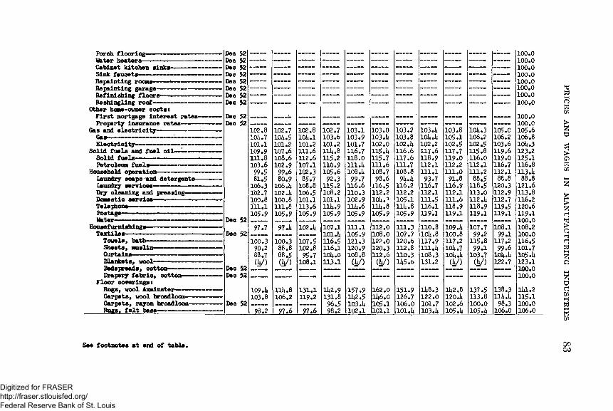
Porch flooring- Water heaters—Cabinet kitchen sinks- Sink faucets- Repainting :Repainting garage— Refinishing floors- Reshingling roof-
Other home-owner costss First mortgage interest rates-Property insurance rates-----
Gas and electricity------------Gas------------------:-------Electricity-
Solid fuels and fuel oil- Solid fuels-----------Petroleum fuels-
Household operation-Laundry soaps and detergents laundry services-----------Dry cleaning and pressing-Donestic service---------Telephone-------- ----- -Postage— — --------—Water--------------------
Housefurnishings- Textiles-Towels, bat Sheets, nuslin- Curtains------Blankets, wool----Bedspreads, cotton-
cotton-Drapery fabric,Floor coverings!Rugs, wool Axminster— Carpets, wool broad loan— Carpets, rayon broad loom-
felt base-
Dec 52 Dec 52 Dec 52 Dec 52 Dec 52 Dec 52 Dec 52 Dec 52Dec 52 Dec 52
Dee 52 Dec 52
Dec 52 Deo 52
Deo 52109 .4 103.8
98 .2
114.8106.2
100.0100.0100.0100.0100.0100.0100.0100.0100.0100.0105.6106.8104.3 123.2125.1 116.8113.4 88.8
121.6113.8116.2 120.6119.1 100.0108.2 100.0116.5 101.7 105.4123.1
' 100.0100.0141.2 115.1 100.0 106.0
See footnotes at end of table.
PRICES AND
WAGES
IN M
ANUFACTURING IN
DU
STRIES
Digitized for FRASER http://fraser.stlouisfed.org/ Federal Reserve Bank of St. Louis
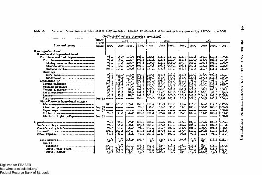
Table 12. Consumer Price Index— United States city average: Indexes of selected items and groups, quarterly, 191*7-58 (Cont*d)
(1947-49=100 unless otherwise specified)
Item and groupOtherindexbases
1950 1951 1952Mar. June Sept. Dec. Mar. June Sept. Dec. Mar. June Sept. Dec.
Housing-ContinuedHousefurni shings— ContinuedFurniture and bedding------------ — 98.9 98.9 105.0 108.9 112.6 113.1* 113.1 112.9 111.8 110.1 110.1 109.6
98.5 98.2 101*.7 108.3 111.1* 112.1 111.5 111.3 110.0 108.0 108.3 107.8Living room suites------------- 97.0 97.5 102.9 106.1 109.6 111.1 109.0 109.9 .109.7 106.8 107.9 106.9Dinette sets— — --- — — --- — — 96.0 93.2 100.9 105.1* 105.1* 106.2 106.1 106.3 101*.1 103.1* 102.9 102.8Bedroom suites— -— ------ -- -- 101.1* 101.3 108.6 112.7 117.1 116.6 117.7 115.5 113.6 111.7 111.7 111.6
Bedding:Sofa beds--------- ----- ------ 98.8 101.0 102.6 10l*.9 110.6 111.2 112.2 111.2 110.6 108.0 108.5 111.2Mattresses--------------------- 99.1 98.9 107.8 115.3 119.7 121.0 120.3 121.0 120.3 119.3 117.3 115.9
> I £' 1 09 r i i i i i i i 1 1 1 95 .1* 9l*.5 97.7 100.5 10l*.0 103.2 101.2 101*2 99.8 98.1 97.9 97.9Sewing machines------------------ 106.1 105.5 107.9 110.8 111.6 112.0 112.0 112.0 111.6 112.0 112.5 lll*.0Washing machines— ----------- 99.0 97.3 102.0 103.6 106.7 107.1* 107.8 i07.6 107.8 107.7 107.1* 107.0Vacuum cleaners— ---------------- 97.8 97.U 98.9 101.5 105.6 106.1 105.5 105.5 107.3 108.2 108.1 108.2Refrigerators— — --- — — — — 98.6 97.1 98.9 101.9 10l*.l 101*. 1 10l*.6 105.0 102.2 98.1 99.6 99.0Ranges—— ——— ———— — — ———— ———— 93.9 93.5 98.7 101.2 108.1* 109.0 106.6 107.5 107.1 106.9 105.0 105.1*Toasters-— -— ------ —-------- Dec 52 -— - -— - 108.6 110.0 105.8 103.1 102.5 102.3 100.5 100.2 100.0
Miscellaneous housefurnishings tDinnerware---------------------- 105.8 105 .1* 105.1* 108.0 111.7 111.9 111* .5 115.6 116.5 116.0 117.0 117.6Aluminum pans— ------------------ Dec 52 ---- — — 95.8 98.3 98.8 98.8 99.1 100.1* 100.2 100.0 100.0Paper napkins— --------- ------- Dec 52 — ---- --- - ---- ---- ---- ---- ---- — — ---- 100.0Toilet tissue-------------------- 9U.0 93.8 96.2 100.3 108.1 107.6 105.6 105.1 10l*.9 103.2 103.9 103.2Electric light bulbs------------- Dec 52 ---- ---- ---- ---- ---- ---- ---- ---- 100.0
Apparel____ ___ -..n , , ..... . ,, 96.8 96.5 99.2 102.2 106.2 106.6 109.3 108.1 106.1* 105.6 105.8 105.1Hen's and boys1-------------------- - 98.1* 98.1 100.1* 102.8 105.9 107.2 110.3 110.1* 108.7 108.3 107.8 107.1*Women's and girls1-— — -- — ---- --- 93.7 93.3 96.2 98.5 102.1 101.7 101*.7 103.0 101.1* 100.5 101.6 100.1*F ootwear------------------------- -- 101.5 102.1 105.2 110.3 116.8 117.8 119.6 117.9 116.1* 115.1* 111* .2 lllwl*Other apparel------------------------ 89.5 . 88.1* 9U.li 99.1 103.8 103.7 100.1* 96.2 92.8 91.3 91.5 92.5Wool apparel---------------------- (V) (h/) 10i*.9 105.7 (V) (V) 120.7 119.6 (h/) (h/) 116.6 111* .3Men's:Topcoats— — — ------ —-------- 100.1 (V) 103.1 105.2 107.6 m 118.1 118.1 116.7 (V) 113.1* 112.6Suits, year-round-------------- 102.0 103.0 103.8 106.6 112.8 lltf.6 120.5 121.3 116.1* 115.1* 113.7 113.3Suits, summer----- ------------ (h/) 102.9 (V) <J/) (1*/) 115.3 (V) (V) (k/) H2.8 (V) (V.)
PRICES AND
WAGES
IN M
ANU
FACTURIN
G
IND
USTR
IES
Digitized for FRASER http://fraser.stlouisfed.org/ Federal Reserve Bank of St. Louis
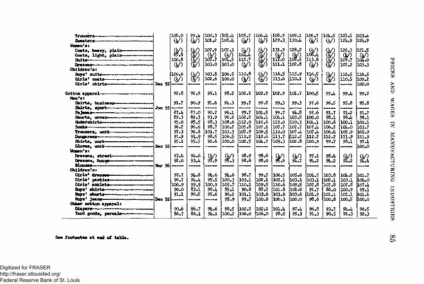
Trousers-- --------Sweaters— -— — — —
Wooes*ssCoats, heavy, plain- Coats, light, plain-Suits-Dresses-
Children's s Boys' suits- Girls* coats-Girls' skirts—
Cotton apparel- Men's:Shirts, business Shirts, sport——— PajaShorts, woven- Undershir Socka-Trousers, work- Dung&rees-Shirts, work- Gloves, work-
Uoasn'stDresses, street— Dresses, house— Blouses-
Children'ssGirls* dresses- Girls* panties- Girls* anklets- Bogrs' shirts— Boys* shorts— Boys' jeans-
Other cotton apparels Diapers—lard goods, percale
100.0(j*/)
Dee 52
Jun 55
Dee 52
Mar 56
Deo 52
.8100.8(V)
100.6(V)
92.8
91.7
Tuh89.395.0 96.297.3 91.995.1
93.1*92.0
92.796.7
100.990.091.1
90.686.7
See footnotes at end of table.
99.U(V)
100.3101.2
101.1*108.1*
105.2(V)
106.1*(V)
108.9129.3,
109.1130.1*
106.7(V)
10U.5(V)
103.512l*.9
103.1* 121* .9
(i/)
<5$
107.9d / )
102.7103.0
107.3Q/>iolT.5
103.0
M112.7(i/)
(| /) 131.9(V)
112.0111.1
128.2<£0
108.5102.8
(V)106.1*113.8(V) 1 !
126.3(ii/)
109.7107.2
121.5(V)
ldT.0103.3
103.8-102.6
106.5100.0
110.8(V) 1 !
116.5113.6
115.9110.1
116.5(U/)
116.5110.5
116.5109.2100.0
92.9 95.1 98.2 102.2 102.9 102.9 101.7 100.5 99.1* 99 .h 99.2
90.9 91.6 91* .3 99.7 99.8 99.3 99.3 97.6 96.5 95.8 95.8
87.089.395.596.6 96.8 91.9 95.5
90.7 93.9 98.398.7
101.798.596.6
96.196.2
108.6100.2103.3106.5100.0
99.7102.2112.0105.8107.9112.2102.5
101.5lOlul112.6 107.1109.5112.6 10U.7
99.7lOU.l112.0107.7 110.0113.7 105.3
9U.8103.5110.3107.7 107.1* 112.2102.8
92.6100.010l*.l107.1*107.1*112.2100.9
91.7 98.1
100.6106.2106.1*112.2
99.7
91.298.1*
100.110U.0105.9111.9
98.1
91.298.1
100.1 103.7105.9111.997.1
100.0
i |
(V)92.9
98.998.6
98.698.0
(V)95.9
(V)95.7
97.19lw2
98.1*9k.2
(V)9H.2
(V)9t.h
9U.89l*.l*99.5 83.190.5
9lu695.5
100.998.1*95.6
911.6100.3105.7
99.196.2 95.9
98.7103.1110.1
90.8 101.1
99.7
99.5102.1109.5 88.2
103.6 100.8
106.5 102.1110.6 101.8 103.6 100.3
105.6103.1109.5 101.0103.6 100.0
10U.5103.1107.891.7
101.998.6
103.8102.1107.8
86.0101.1100.8
10U.2103.1 107.8’ 100.9101.1 100.5
101.710l*.0107.1*99.1
101.1100.0
86.786.1
9li.69l*.l
98.5100.2
102.2106.0
102 ;2 106.0
101 .U 98.Q
97.1*95.3
96.891.3
93.790.5
9k.k91.3
96.592.3
00Ox
PRICES AND
WAGES
IN M
ANUFACTURING IN
DU
STRIES
Digitized for FRASER http://fraser.stlouisfed.org/ Federal Reserve Bank of St. Louis
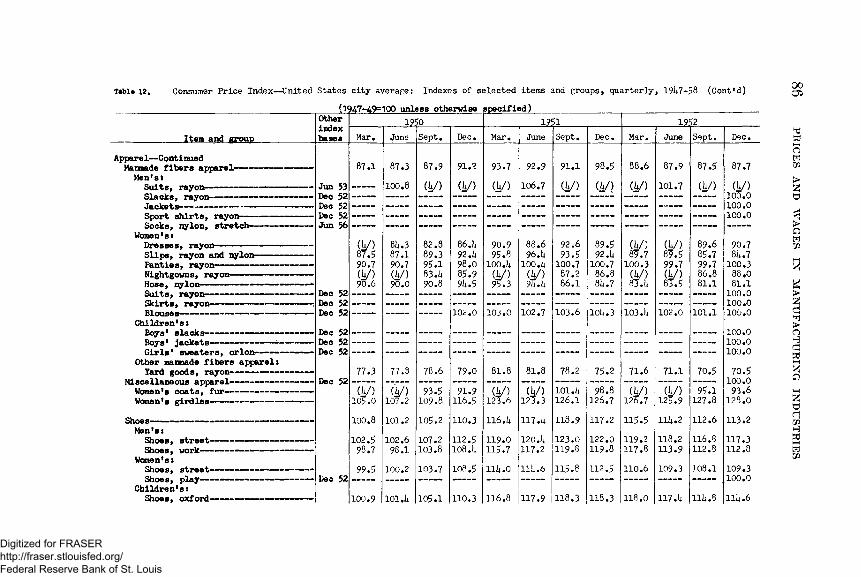
Table 12. Consumer Price Index— United States city average: Indexes of selected items and groups, quarterly, 19U7-58 (Cont’d) 00oa
Item and croupOtherindexbases
19!?0 1951 1952
Mar. June S e p t. Dec. Mar. June Sept. Dec. Mar. June Sept*
8 7 .1 8 7 .3 8 7 .9 91.2 9 3 .7 9 2 .9 9 1 .1 9 8 .5 88.6 8 7 .9 8 7 .5
Jun 53 Dec 52
---- 100.8 (h/) (V) (V) 1 0 6 .7 (V) (h/) (V) 1 0 1 .7 (V)
Jun 56
Dec 52 Dec 52 Dec 52
W )8 7 .5 9 0 .7 ( i / )90.6
8U.38 7 .190.7W )90.0
8 2 .88 9 .39 5 .183.U90.8
86. h 92.1*9 8 .08 5 .99U.5
90.99 5 .8
100.1*r ,
88.6 9 6 .ib
100.it (U /) 9ll.li
92.69 3 .5
1 0 0 .787.286.1
8 9 .5 92.h
100 .7 86.8 8ii.7
(V)8 9 .7
1 0 0 .3(V)8l . l i
(V)8 9 .5 99 .7(V)8 1 .5
89.685 .799 .786.8 81.1
---- ---- ---- 102.0 1 0 3 .0 1 0 2 .7 1 0 3 .6 10iw3 1 0 3 . h 102.0 101.1Dec 52 Dec 52 Dec 52
Dec 527 7 .3 77 .3 78.6 7 9 .0 81.8 81.8 78.2 7 5 .2 71.6 7 1 .1 7 0 .5
i< £ .oTh/)107.2
9 3 .5109.8
9 1 .9116 .5
7 y )123.6
Th/)1 2 3 .3
101 .a 126.1
* 9 8 .81 2 6 .7
Th/)1 2 6 .7
"(V)1 2 5 .9
9 5 .1127.8
100.8 101.2 1 05 .2 110 .3 116. k 1 1 7 .ii 1 1 8 .9 11 7 .2 1 1 5 .5 i i i ; .2 112.61 0 2 .5
9 8 .7102.6
9 8 .11 07 .2103 .8
1 1 2 .5 108 .h
119.0115 .7
120.li1 1 7 .2
1 2 3 .01 1 9 .8
1 2 2 .01 1 9 .8
1 19 .21 1 7 .8
118.2113.9
116.8112 .8
Deo 529 9 .5 100.2 10 3 .7 10 8 .5 lll i .O nil.6 1 1 5 .8 112.5 110.6 109.3 1 0 8 .1
1 0 0 .9 101.U 1 0 5 .1 110 .3 11 6 .8 1 1 7 .9 1 1 8 .3 1 1 8 .3 1 1 8 .0 117 J4 nii.8
Apparel— ContinuedManraade fibers apparel- Men*st
Suit8, rayon—Slacks, rayon------- — — ---Jackets---------------------Sport shirts, rayon---------Socks, nylon, stretch-------
Women's:Dresses, rayon— — ----------Slips, rayon and nylon------Panties, rayon-Nightgowns, rayon- Hose, nylon Suits, rayon-Skirts, rayon- Blouses-
Children'ssBoys' slacks--Boys' Jackets— ------ ----—Girls* sweaters, orIon-----
Other manmade fibers apparels Yard goods, rayon----------
Miscellaneous apparel- Women's coats, fur- Women's girdles-
Shoes-Men'stShoes, street----Shoes, work------
Women'ssShoes, street---- — --------Shoes, play— ---- — -------- -
Children's:Shoes, oxford— ---- ---------
8 7 .7
(V)100.0100.0100.0
9 0 .781+.7
1 0 0 .3 88.0 81.1
100.0100.0100.0100.0100.0100.0
7 0 .5 100.0
9 3 .6128.01 1 3 .2
1 1 7 .3 112.8
1 0 9 .3 100.0
llli.6
PRICES AND
WAGES
IN M
ANUFACTURING IN
DU
STRIES
Digitized for FRASER http://fraser.stlouisfed.org/ Federal Reserve Bank of St. Louis
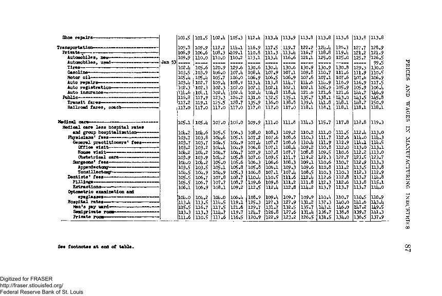
Shoe repairs-Transportation-
Private- Automobiles, new—Automobiles, used- Tires-Gasoline- Motor oil- Auto repairs-Auto registration- Auto insurance— —
Public-Transit fares-Railroad fares, coach--
Medical care-Medical care less hospital rates
and group hospitalization—Physicians1 fees---General practitioners' fees- Office visit-------------House visit— — Obstetrical care-
Surgeons* fees— —Appendectomy-Tonsillectony-
Dentists' fees- Fillings-Extractions-
Optonetric examination and eyeglasses-
Hospital rates-Hen's pay ward— Seni private rooa- Frivate root— —
Jan 53
101.5 101.5 102.1* 105.3 112 .k 113.U 113.9 113.8 113.8 113.8 113.8 113.8109.3 109.9 112.7 llli.l 116.9 117.5 119.7 122.2 12l*.l* 126.3 127.7 128.9106.9 106.6 108.3 J.09.1 110.8 111.3 113.1* 116.7 118.8 119.1* 121.2 121.9109.9 110.0 110.0 110.2 113.1 113.1* 116.6 121.1 125.0 125.0 125.7 126.5oo cf102 .U 105.6 120.9 129.6 130.6 130.1* 130.6 130.9 130.9 130.8 129.3
77 •?130.0
103.5 103.9 106.0 107.14 108.1* 107.9 107.1 109.8 110.7 111.6 111.9 110.5105.1* 105. h 105.7 106.0 106.9 106.5 106.9 107.6 107.1 107.6 107.6 106.9103 .1* 102.7 109. h 108.9 113.14 113.8 11U.7 111* .6 111*.9 116.9 116.9 117.5102.3 102.3 102.3 102.0 102.1 102.1 102.1 102.1 105.9 105.9 105.9 106.1*11U.6 10U.1 102.)4 102. h 102.1* 10l*.8 118.1* 121.6 121.6 121.6 11*1* .7 11*6.9116.8 117.9 123.3 126.2 131.6 132.5 135.1 135.7 138.1 11*3.0 11*3.5 11*5.8117.2 119.1 125.5 128.7 135.9 136.0 138.8 139.1* 11*1.8 11*8.1 11*8.7 150.9117.0 117.0 117.0 117.0 117.0 117.0 117.0 118.1 118.1 118.1 118.1 118.1
105.1 105.1* 107.0 100.0 109.9 111.0 111.8 111*.3 115.7 117.8 118.8 119.310l*.2 lOli.6 105.5 106.3 108.0 108.3 109.2 110.2 111.0 111.5 112.1* 113.0103.7 103.8 10iu6 105.1 107.2 107.6 108.6 110.3 111.7 112.6 lli*.0 111* .3103.7 103.7 10lw5 10U.9 107 .li 107.7 108.6 110.1* 111.9 112.9 lll*.l lll*.5103.2 103.2 lOii.l* 10U.9 106.8 107.1 108 .U 109.2 110.8 112.0 113.0 113.110l*.2 10l*.2 10U.7 10U.7 107.9 107.8 107.7 108.8 109.5 110.6 112.2 113.0103.9 103.9 10li.2 105.8 107.6 109.5 111.7 119.2 122.3 122.7 123.5 123.710l*.0 10l*.2 105.0 105.6 106.3 106.6 108.3 109.1 110.6 110.7 112.9 113.3103.5 103.5 105.1 105.8 105.8 106.1 109.3 109.6 110.8 111.2 113.5 113.810U.5 10U.9 10l*.9 105.3 106.8 107.1 107 .1* 108.5 110.3 110.3 112.3 112.9105.5 106.7 107.8 108.7 110.U 110.5 111.6 112.1* 112.6 112.8 113.7 111*. 8io5.5 106.7 107.7 108.7 109.6 109.8 111.2 111.8 112.3 112.6 113.8 115.1106.1 106.9 108.1 109.2 112.5 112.1* 112.8 lll*.2 113.7 113.7 113.7 lll*.0ioU.o 10l*.2 lOii.O 106.1* 108.9 109.1* 109.7 109.9 110.1* 110.7 110.5 110.9113.1* 113.5 11U.5 119.1 125.3 127.3 127.9 131.2 137.3 11*0.0 11*1.6 11*3.1*115.5 116.7 117.5 121.6 129.7 131.7 132.5 135.7 11*3.1 11*6.0 11*7.2 11*9.5113.3 113.3 llli.7 119.7 12U.7 126.8 127.6 131.1* 136.7 138.8 139.7 11*1.3111.6 110.5 111.6 116.5 120.9 122.9 123.2 126.5 131.5 131* .0 136.5 137.9
See footnotes at end of table* 00
PRICES AND
WAGES
IN M
ANUFACTURING IN
DU
STRIES
Digitized for FRASER http://fraser.stlouisfed.org/ Federal Reserve Bank of St. Louis
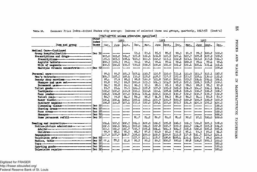
Table 12, Consumer Price Index— United States city average: Indexes of selected items and groups, quarterly, 1957-58 (Cont'd)(1947-49=100 unless otherwise specified)_______________
0000
Item and groupTO»rindexbases tar* June S ept. Dec
1950Mar. June Sept* Dec
1951Mar* June S e p t, Dec
.1952
Medical Care— Continued Group hoepitalisatioPrescriptions and drugs— ---- -Prescriptions- Aspirin tablets-Milk of magnesia---Multiple vitamin concentrate-
Personal care- Men's haircuts-Beauty shop services--Shampoo and wave set-Permanent wave---
Toilet goods-------Toothpaste- Face powder- Toilet soa]Razor blades* Sanitary napkin; Cleansing tissue-Shaving cream---Face cream— — ---Shampoo— —— — — ——Hone permanent refill-
Reading and recreation-----Moti on-pi cture admissions- Adults- Children-
Newspapers-Television sets-Radios, table--Toys-
Dec 52
Dec 52
103.0105.110 0 .3100.5
9 9 .110 5 .7
98.5 9 9 .89 6 .79 3 .7
100.2 1 0 6 .5
8 0 .7 100. k106.8
Sporting goods— --Television repairs-
Dec 52 Dec 52 D*c 52 Dec 52 Dec 52
Dec 52 Dec 52 Dec 52 Dec 52 Dec 52
103 .21 0 5 .5 100 .31 0 0 .5
99 .2107 .2
9 7 .99 9 .59 5 .8 9 3 . 5
100.2106.8
7 9 .8 1 0 0 .5 1 0 6 .8
105.7108.5
99.141 0 0 .5
1 01 .31 0 8 .5 98.2 99 .89 6 .1 9 5 .5
1 0 0 .910 7 .085.2
1 0 0 .5 1C 7.5
8 3 .11C 5.81 1 0 .5
9 9 .51 0 0 .5
1 0 7 .5 1 1 6 .298.8
100.69 6 .3
1 0 5 .3 110.11 3 0 .5
8 9 .31 0 0 .5112.6
83.6106.6111.6
9 9 .51 0 0 .5
1 1 0 .7 118.2 1 0 0 .9 1 0 3 .3
9 7 .5107.8 110.61 3 1 .5
9 5 .51 0 0 .5 122.0
8 5 .5 106.8 112.2
9 9 .5 100.6
110.8118.2101.81 0 5 .3
9 8 .51 0 7 .91 1 0 .51 3 2 .5
9 5 .81C0.91 2 2 .5
8 5 .5 1 0 7 .5 1 1 3 .1
9 9 .5 101.0
110.01 1 6 .5 102.0 1C 5.7
9 8 .31 0 5 .9108.6 1 3 2 .5
8 9 .71 0 0 .9 122.0
9 0 .3 1 0 7 .5 112.8
99 .li 101.2
111.1122.01 0 3 .5 1 0 7 .0
3.51 0 5 .9108.61 3 2 .7
3.91 0 0 .9123 .7
9 1 .91 0 7 .71 1 3 .5 100.01 0 1 .5
111.01 2 3 .51 0 3 .5 1 0 7 .1
9 8 .51 0 5 .9106.6 1 3 2 .7
8 6 .7100.9 125.6
1 1 1 .71 2 8 .51 0 5 .5 1 0 8 .3
9 8 .91 0 5 .21 0 6 .71 3 2 .7
8 5 .11 0 0 .9125.0
1 0 5 .5102.6 1 0 3 .1
9 9 .91 0 7 .9
88.5
10 2 .5100.6 101.2
3.1 1 0 7 .9
8.1
1 0 2 .7 103,.1101.7
5.7fL08.7
9 1 .6
8 5 .2
1 0 5 .1102.01 0 2 .7
9 8 .7108.01 1 7 .9
9 5 .2
85.21 0 7 .01 0 5 .5105.6
9 7 .51 0 9 .01 2 3 .1
9 9 .2
8 5 .2
1 0 6 .5 102.81 0 5 .5
9 3 .010 9 .6 118.5
9 9 .5
85.2105.81 0 2 .71 0 5 .392.2
109.6108.6100.2
85.2
1 0 6 .5 1 0 2 .91 0 5 .5
9 2 .5112.81 0 8 .5 100.0
9 0 .2
1 0 6 .31 0 3 .71 0 5 .1
9 5 .1112.8105 .1
9 9 .8
100.21 0 7 .9113.699.1*
1 0 1 .5
112.11 3 0 .0 105.1*1 0 8 .7
9 8 .31 0 5 .1106.8 1 3 2 .7
8 3 .81 0 0 .9125.2
9 7 .1
106.810lw8106.6
9 3 .31 1 5 .71 0 0 .7 1 0 0 .5
100.0
1 0 7 .3 1 0 3 .9 105.6
9 3 .2 120.2
9 9 .21 0 0 .3
100.01 0 8 .5 Ulu3
9 9 .5 101.li 100.01 1 2 .51 3 1 .51 0 5 .51 0 9 .1
9 7 .91 0 5 .11 0 6 .71 3 2 .7
8 3 .71 0 0 .9125.2 100.0 100.0 100.0 100.0 100.0108.01 0 5 .01 0 5 .6
9 5 .5121.1 100.0 100.0 100.0 100.0 100.0
PRICES AND
WAGES
IN M
ANUFACTU
RING
IND
USTRIES
Digitized for FRASER http://fraser.stlouisfed.org/ Federal Reserve Bank of St. Louis
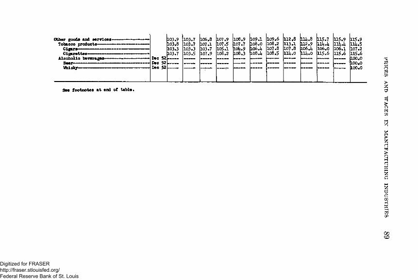
Other goods and services- Tobacco products-
Cigar8-Cigarettes-
Alcoholic beverages- Beer—Whisky-
Dec 52
PL03.9103.8103.3103.7
103.7103.7 103.3 103.5
106.8107.1103.7107.9
107.9107.5105.1108.2
108.9 107.7104.9 108.3
109.1 108.0 106 .4 108.4
109.6108.2107.8108.5
112.8113.1107.8114.0
114.8112.9 106.4 114.0
115.7114.4106.0115.6
115.9114.4106.1115.6
Dec 52 Deo 52 ------- ------- ------- ------- ------- -------- ------- ------- -------
11U.5107.2115.6100,0100.0100.0
See footnotes at end of table.
00CO
PRICES AND
WAGES
IN M
ANUFACTURING IN
DU
STRIES
Digitized for FRASER http://fraser.stlouisfed.org/ Federal Reserve Bank of St. Louis
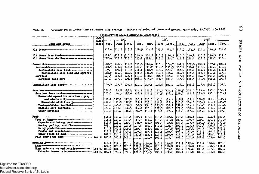
Table 12. Consumer Price Index— United States city average: Indexes of selected items and groups, quarterly, 191*7—58 (Cont*d; CO
It— and groupAll iteaa-All items lass food-All iteaa lass ahalter-Coanodities-Nondurables-Nondurablas lass food-Nondurable# lass food and apparel-
Durables-Durables lees cara-
Cc— nrtltles lass food-ServJoes-Servioee leas rent-Houaehold operation services, gas,
and electricity-Household utilities j/-
Tra exportation aervloea Hadioal oare servicee- Other aervioea-------
FoodFood at hcaa-» — ........ —
Cereals and bakery products---Heat a, poultry, and fish-Dairy products----------Fruits and vegetables—Other foods at hews ■ ---
Food awajr fro« hone-------HousingRent----------— — - ----Hons Maintenance and repairi Exterior house paint-----
(1947-49=100 unless otherwise specified) Other
Jan 53
Dae 52 Dee 52
113.6
115.1 112 .1*
110*7no.5109.7 lliu6 113 J*107.3
110.0122.7123.3
116.1 111.0 11*5.0122.3 112.14
111.7111.3117.7 107.1*110.3115.5109.1100.1116.3121.7100.6100.3
JLS&L.June. Sept.llli .5 115.2115.5 113.3
111.5111.6 109.6 ill*. 5112.9107.1
116.3 U3.5
111.7 112.1110.7115.9112.3106.9
109.3 110.2123.3 12l*.3117.2111.811*5.8123.7 113.2
113.7113.7118.9111.3107.5121.7110.9 100.2U7 .1*123.3101.6
99.9
125.1*125.6
117.3112.7150.3 121*.5 lli*.l113.8113.5120.3113.5109.6 106.6 116.7 101.0118.1*126.0103.099.6
Dec. Mar. June Sect. Dec.llli.9 111*.8 115.1 lllu7 llh.3 111* .3116.6113.1*
111.0111.5 111.1116.6 110.9 106.1*
116.5113.1
110.6111.2110.9 116.8 110.1105.9
116.3 113.1*
110.3 112.0 110.1* 116.1108.7103.7
116.3112.7109.7111.3 10.1* 116.2 106.2 102.9
116.6112.2
109.1110.1 110./* 116.0 107.0 102.5
116.)*112.?109.0110.2110.2116.1*106.2101.8
116.3112.3108.9 110.1*109.9 116.0 10l*.7 101.0
110.0 109.1* 108.6 107.7. 108.1 107.6 107.0126.2126.3
118.3113.5150.5 126.0 111* .7
112.3111.7120.9107.8110.3109.2113.5 101.7
118.9127.6103.2 102.6
126.8126.9118.6 113.8 151*.0 126.1* 111* .7112.1111.1*121.2109.5 108.0 107.8 112.3101.9119.0128.0103.6 103.5
127.3127.5
117.7 112.2153.3127.3 116.1113.8113.3121.3 111.1102.9117.1115.2102.3
118.9128.3103.6102.7
128.1 123. h
117.9 112.1*153.9 128.2 117.1*
112.1*111.6122.6106.7105.8110.5 116.0102.7
119.5128.8 103.8 102.7
128.5128.7
118.1*113.1 151* .1*129.3117.3
110.1*109.2123.3 102.2106.8 108.1* 112.0 102.8
119.7 129.1*103.7 103.1
129.0129.2119.1 111* .2 151*.3 130.6 117.1*110.8109.7123.9102.3105.1 112.0111.9102.9
119.6130.010U.1*103.0
129.6129.9
120.9115.3153.7130.8 118.1
111.3110.3 121*.0103.8 10l*.l119.5107.7102.9
119.7 130.1*105.8103.5
11/*.9 lll*.7
116.9112.7
109.2111.1111.1117.1103.7101.1
117.6112.1*
108.7110.2111.6117.9105.1100.3
107.3 108.1
130.i*130.3
121.3115.3153.3 131.6119.3
111.6 110.U 121*.0103.5106.5 110.2 lll* .l103.6
120.1*130.5107.1103.8
130.9131.3
122.3115.9153.6 133.1*119.3
109.5107.9123.9 91* .6107.7110.7113.7 101*.3
120.8 131.1 107.7 101*.3
PRICES AND
WAGES
IN M
ANUFACTURING IN
DU
STRIES
Digitized for FRASER http://fraser.stlouisfed.org/ Federal Reserve Bank of St. Louis
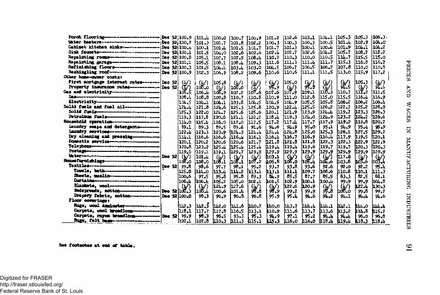
Porch floorin g— ■■— — — —Wfcter httt«ra--------------------------Cabinet kitchen sinks— --------Sink faucets---------------------- —Repainting roe— - —.....Repainting garage— — ——Refinishing f lo o rs—--------- -----Re shingling roof— ' ......... . ■
Other hqns owner costst F irst aortgtge interest rates* Property insuranoe rates— —
Gas and e le c tr ic ity -------------------Gas----------------- ------------------------Elect r i c ity— — — -------------
Solid fuels and fuel o i l——Solid fuels-----------------------------Fstrolftua fu e ls - — — - -
Household operation— - —*.... ■Laundry eoapa and detergents- laundry ssrvioes— ——Dry cleaning and pressing— Doaestio service— — ■■ ■■ ■ . . Telephone— ■ — — — Postage— ■Utter- ' ............... . ■ — .......... ■■ .i.
Housefurni A ings—--------- ■■---------Textilss—- ■' - - - ....... - ■ ■ ■—
Towels, bath— ...- ................. .Sheets, Muslin- ......Curtains-- ------—■ ■ ■Blankets, wool---------------------Bedspreads, oottoo— —Drapery fab ric , oottoo--------
Floor coveringst Rugs, wool Aaainster—— Carpets, wool broadloci Carpets, rayon broad loan Rugs, f e l t base- ■ »■■
See footnotes at end of table.
Dec 52 100.9 101.4 100.0 100.7 100.9 101.2 102.6 103.1 104.1 105.3 105.3 106.3Dec 52 100.7 101.3 101.7 101.8 102.2 100.3 100.3 100.3 100.5 101.4 102.9 104.0Deo 52 100.U 100.1 101.4 101.5 101.7 101.7 101.3 100.1 ioo .4 101.9 104.1 104.2Dec 52 100.1 101.5 104.0 102.6 102.6 102.4 102.7 102.6 104.2 105.7 108.7 112.7Dec 52 100.8 105.1 107.7 107.9 108.4 110.2 110.3 110.0 110.5 114.7 115.5 115.0Deo 52 101.1 105.5 108.1 108.4 109.3 111.6 111.3 111.4 111.7 115.3 116.8 116.7Deo 52 100.3 101*5 104.4 103.4 103.0 104.5 106.7 106.5 106.2 107.8 110.0 110.8Dec 52 100.9 102.3 106.9 108.2 109.6 110.6 110.6 111.1 m . 5 113.0 115.9 117.2
DecDec
5252
cy>m
(V)1CX5.0
105.8(4/) (V)
100.0 (V)m
<y)95.9
105.0(V)
(4/)95.3 n
(y>94.5
105.3(V)
(y)94.b
106.5 106.4 106.9 107.2 10/.6 107.6 107.9 109.1 110.3 110.7 111.2 111.5108.ii 108.8 109.8 110.7 110.8 110.9 111.0 112.8 115.0 115.5 116 J* 116.9104.5 104.1 104.1 103.8 104.5 104.5 104.9 105.5 105.8 106.2 106.2 106.4124.4 121.8 124.6 125.3 125.8 120.9 122.4 125.5 126.2 122.7 125.2 128.0125.3 122.0 124.7 125.6 125.6 120.1 121.9 123.9 124.4 119.7 123.3 126.3119.3 117.8 120.6 121.1 122.2 118.4 119.3 124.0 124.9 123.2 124.2 126.6114.0 115.4 116.0 117.0 117.5 117.2 117.4 117.7 117.9 119.2 119.8 120.789.1 89.3 89.5 89.6 91.6 94.6 94.9 95.0 95.1 94.9 95.4 95.9
122.4 123.3 123.9 124.3 124.4 12U.4 124.8 125.0 125.3, 126.1 127.5 129.7114.1 116.6 116.6 116.4 116.1 116.4 116.7 116.9 116.4 117.9 119.5 120.1120.1 120.2 120.6 120.6 121.7 121.8 121.3 121.8 122.3 122.3 122.9 122.9120.8 123.2 125.4 125.4 125.4 119.4 119.4 119.6 119.7 119.7 120.3 120.3119.1 119.1 119.1 129.7 129.9 129.9 129.9 129.9 129.9 129.9 129.9 129.9
Deo 52 (V)1CW.0
101.4108.0
(4 /)106.1 (y>108.1
d/)107.2
103.1105.8
(V)1<*.0
cy>icT.4 (V)104.6
117.8103.8
(V)103.6 s a
Deo 52 99.8 98.6 97.7 98.1 95.2 93.7 93.8 93.6 92.6 92.0 92.2 95.4115.0 114.0 113.4 114-2 113.1 1X3.1 111.1 109.7 108.6 110.8 110.1 111.3100.6 97.5 95.8 95.8 89.3 54.9 85.5 87.7 85.5 83.3 82.5 8Q.1106.4 106.4 105.2 105.0 102.1 L01.5 102.9 100.1 ioo .4 99.9 99.9 104.8
Deo 52m
100.3 (V)100.4
124.9100.6127.6101.4 <y>98.8
<y>96.9
122.699.2
120.?99.9
<y>99.8
<y>100.0L22.499.8
130.399.7
Deo 52 100.0 98.3 96.9 96.3 96.8 95.9 95.4 94.6 94.2 94.1 94.4 94.6
142.3 142.3 142.0 141.6 140.7 L40.0 143.7 144.4 lii4.1 142.1 L44.0 144.4118.1 117.7 117.8 116.5 113.1 L10.9 111.6 113.7 113.6 113.2 114.8 115.7Deo 52 99.9 98.3 96.5 93.3 95.3 94.9 97.1 95.2 94.4 94.4 96.0 96.8
107.1 107.8 110.3 111.3 115.1 L15.3 116.0 116.0 118.4 L19.4 L18.3 118.4
CO
PRICES AND
WAGES
IN M
ANUFACTURING IN
DU
STRIES
Digitized for FRASER http://fraser.stlouisfed.org/ Federal Reserve Bank of St. Louis
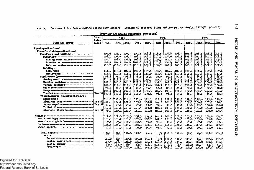
Table 12. Consumer Price Index— United States city arerape: Indexes of selected items and groups, quarterly, 19^7-58 (Cont'd)CObo
It— aal groupHousing—Continued
.Housefurnishlngs—ContinuedFurniture and bedding-------
Furniture-Living room suites Dinette sets- Bedroom suites-
BeddingsSofa beds— -Mattresses--- — —
Appliances 2/— — -— Sewing machines— —— - Washing machines— — Vacuum cleaners— ----
(1947-49=100 unless otherwise specified )Otherindexb t f
Refrigerators- Ranges-Toasters— — — — — —
Miscellaneous housefurnlshingst Dinnerware-Alumlnum pans--- — — --Paper napkins-- -------Toilet tissue— ---- -Electric light bulbs-—
Mar.
Dec 52
109.6108.1107.7 103.9110.7111.5 113.097.511U.1105.8 109.398.0
105.2100.5
DecDecDec
Men's and boysrWomen's and girls'- Footwear-Other apparel-Wool apparel— -- -—Men'siTopcoats---------Suits, year-round-Suite, summer-- —Trousers--- -----
118.0101.5 . 99.0103.5
52j 99.710U.7107.399.6m . ?92.1.(J±/>
111.2113.6(V )
1CT.7
1953June Sept. Dec.
110.1108.9 108.0 10U.9 112.0110.1112.797.0115.5 106.0112.896.0107.1 10C .8118.0102.1 99 .a103 .U 110.110U.6107.299.2 115.392.3(U/)(J/>113.7
113.9101.5
109.7108.7 108 .U lOJi.l 111.2109.1m .a 96.8
116.U 106.0 112 .h 96.1
107.0101.7118.8 101.999.U
103 .a111.5105.3107.5100.5115.3 92.5116.0112.8llli.8<U/)103.6
109.3 108.1 108.6 102.6 110.7109.6111.196.1119.0105.3113.1 9U.6
108.1101.5121.0 103 .a99.2
103.5 111.1105.3107.6100.5116.190.9
115.1115.0n a.8(a/)
lda.i
Mar. June Sept. Dec.
108. 5107 .a 108.2102.7109.1109.8 111.095.1119.7ioa.2113.693.1
108.3100 .a
122.1103.899.2
103.0111.0ioa.3107.299.0 116.190.0(a/)
na.3115.3 116.5-I loi.a
_12$k
108.6107.3109.3lOl.a108.7108.5111.5 92.9
119.2103.1109.988.810U.596.3122.3 ioa.299. a103.6 109.aioa.2107.098.5116.3 91.0
(i/)
115.7115.0ioa.i
108.8 107.6 111.2 ioi .a107.5109.a111.691.3118.5102.9 112.8
88 06103.596.3122.9 ioa.698.5
103.0109.3ioa.3i»s.a99.0116.5 90.9116.0112.6 li5.8(a/)103.6
108.7 107.3111.8100.5 106.8
109.1112.190.1117.7102.5110.886.7
ioi .a95.7
122.8ioa.699.1
101.8 115.2ioa.3106.599.0 116.991.1
na.o
112.5 •115.7(a/)103.6
Mar. June
107.6105.9 109.699.0
106.a109.9111.7 89.a
115.7 101.0 110.187.7
102 .a86.3
12a.3105.1 99.6
102.1 118.2103.2 105.6 97 .a116.7 90.li(k/)
111.1,116.1na.oioa.5
SepL.— Dei
106.3ioa.3108.5 99.7102.5108.7112.a 88.6 116.1100.6 106.286.9101.986.1125.0106.5 99.5
101.0 121.a103.2105.6 97.2
117.1*90.1
(V>(a/)110.0
i3 a.7105.0
106.6ica.8109.7 99.9
102. a
io9.a111.7 87.8
n5.a100.7107.8 82.3
ioa.285.5
123.6107.7 100.0101.8 120.0ioa.6105.899.5
118.191,0U5.2112.6116.1;(a/)
105.5
106.7 ioa.7109.1 100.9102.3109 .a 112.6 35.9115.398.0
106 .a78.0
101.2 8a.3
i2a.7120.1100.0101.0120.5ioa.7106.199.1119.891.1
iia.5112.6 ll6.a(a/)
10^.5
PRICES AND
WAGES
IN M
ANUFACTURING IN
DU
STRIES
Digitized for FRASER http://fraser.stlouisfed.org/ Federal Reserve Bank of St. Louis
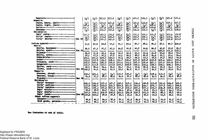
Sweaters-— ---------Women's*Coats, hasty, plain— — Coats, light, plain— —Suite— ----- --- — —
----— --------— -Children’#*
Boys' suit*— — --- —Girls* ooats— --------Girls* skirts-
Cotton apparel-— — --Han's tShirts, business----Shirts, spo<rt— — ■— Pajanas-Shorts, wove Undershirts- Sock*Trousers, work- Dungarees*Shirts, work< Gloves, work-
Wasen'stw itDresses, street Dresses, hous~ Blooni-
Children'stGirls' dresses-
Deo 52
Jun
117.7(U/)(5/)99*6
96.6
Deo 52i
Mur 56.
Girls1 panties-Girls* anklets- Boys' shirts-Boys' shorts- Boys' jtus-
Otbsr ootton apparels Diapers— - ■— ■■■■■ Tsrd goods, psroale-
52
lOli *2 x03.6 105 .h 96.9
102.U 100 <6
(U/) :123.3 :123.1 (U/) (h/) :120.7 1L21.3 (V ) (h/) :121.2 1L21.1*
nW )
123.9 (U/)
107.9122.6(U/)
103.1<y>
105.5109.0
(£/) :122.6 ] U /)
106.0 :L16.9 (V ) :L02.2 :
(V )105.0100.6
(£/) : (V )
119.1 ](W)
10T.h :L17.7(V)
LOO.O(5/) 100.7 loS.i (h/) ( y ) lou.o :L03.3 (V ) cn/) 107.7 :L08.6
a / ) 120.1 120.5 121.2 (V ) 121.2 :122.1 121.8 (V ) 122.1* :122.8110.2 106.9 (V) (J/) 110.7 :106.1 (V ) 112 .li 106.7
(h/) 100.3 101.9 (y ) d /) 101.5 :101.5 <£/) ( ! / ) 102.0 103.0
99.6 99.8 99.S 99.3 99.1 98.5 98.14 98.3 99.1 99.7 100.0
97.3 97.5 97.9 96.8 96.8 96.5 96 J* 96.2 95.9 95.6 95.7• • — — - — - - 100.0 101.6 102.1
91.8 92.li 91.6 90.7 90.6 90.5 90.6 90.8 90.6 90.6 90.797.9 97.li 97.5 96.1} 96.2 96.5 95.8 9U.9 95.1 95.1* 96.0
100.0 100.7 100.6 99.1i 99.7 99.6 99.5 99.6 99.5 99.6 99.9103.8 10U.5 lQli.6 106.7 106.2 105.9 105.8 105.8 105 .li 106.5 106.5106.1 iot.5 101* .0 103.li 103.1 102.9 102.6 101.3 101.2 101.li 101.8110.6 110.7 110.6 109.3 108.8 106 .lj 106.1* 106.2 106.1 106.3 106.396 .U 96.1i 96.6 96.1 95.1 92.6 92.5 92.1 92.9 9U.2 95.096.6 96.il 95.9 95.0 9lu8 91.7 91.7 91.5 *90.7 91.0 91.2
103.195.2
(1/)95.0 n105.79U.9
ss i
H 1
( V )95.2 (V )9U.2
108 .U 914.1
111.3914.2
<y>9C.9
101.2 107.3 107.5 108.7 108.1 106.9 106.8 103.8 101.6 10U.8 105.310U.0 103.9 loU.5 103.1 103.0 103.6 10U.7 10U.3 102.8 105.3 L06.il105.3 107.3 107.9 107.9 107.5 107.3 107.3 106.7 10U.8 105.1 105.198.8 99.5 99.3 99 .1* ,97 .U 95.9 95.1 95.3 9U.7 9U.3 95.2
102.3 102.8 102.9 103.1 102.9 102.8 101.0 98.3 98.3 98.5 99.1100.2 98.9 97.8 96.3 95.9 9U.9 95.2 93.9 93.5 92.1 92.1i96.7 96.0 88.6 87.2 91.2 90.9 91.1 91.1 91.0 91.5 91.592.1 92.2 91.7 91.0 91.1 91.2 91.5 92.2 91.0 91.5 91 Ji
See footnotes at end of table.
OO
PR
ICE
S AND
WA
GE
S IN
MA
NU
FA
CT
UR
ING
IN
DU
ST
RIE
S
Digitized for FRASER http://fraser.stlouisfed.org/ Federal Reserve Bank of St. Louis
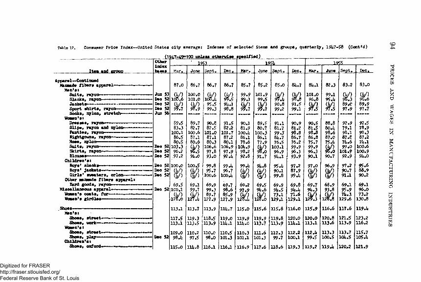
Table 12. Consumer Price Index— United States city averaget Indexes of selected items and groups, quarterly, 191*7-58 (Cofit*d)
(1947-49=100 unit as otherwise specif ied^
CD
JttfiLsad-msu?-Apparel-—ContinuedNanmade fibers apparel- Men'siSuits, rayon-Slacks, rayon-— —Jackets-----------Sport shirts, rayon-Socks, nylon, stretch---
Vomen'stPresses, rayon— --------Slips, rayon and nylon— Panties, rayon - - Nightgowns, rayon- Hose, nylon-Suits, rayon— Skirts, rayon- Blouses-
Children'stBoys' slacks— —Boys' Jackets—Girls' sweaters,
Other mannade fibers apparels lard goods, rayon---- - -— —
orlon-
Nisoellaneous apparel- Women's coats, fur- Women's girdles—
Shoes— < Hen'stID'IIShoes, street- Shoes, work
women's sShoes, street- Shoes, play—
Children's! Shoes, oxford-
Other 1953 1951* __________ 1955indexbases Mar. June Sept. Dec. Mar. June_ Sept. Dec. Mar. June Sept. Dec.
87.0 86.7 86.7 86.7 85.7 8 5 .2 8 5 .0 ei*.7 81*.1 82.3 83.2 83.0
Jun 53 Dec 52 Deo 52 Deo 52 Jun 56
(V)1 0 0 . 6
(£/)99.7
1 0 0 .01 0 1 . 0
<i/)98.9
(k/)1 0 0 . 195.599.3
(y>99.5 91* .1 9 8 .8
99.999.1<y)99.7
101.999.5cy>99.7
(y>99.1*9 0 .899.2
(y>98.891.599.1
1 0 1 . 09 6 .8<y)97.5
99.195.1*m
(y>96.389.097.9
c y )9 6 .689.997.7
Deo 52 Deo 52 Dec 52
09.5 83.3
1 0 0 . 186.580.5
103.39 6 .2,97.2
89.782.7
1 0 0 .687.1 8 0 .6 (V) 96.5 91* .0
9 0 .e82.5
1 0 1 . 087.180.3
1 0 6 .697.893.0
91.582.2
101.78 7 .28 0 . 1
106.997.992.1*
9 0 .181.9
1 0 0 . 1*8 6 . 17 8 .6
10l*.99 8 .29 2 .8
89.580.7,
100.38 6 .177.9U /)98.091.7
91.181.799.5 81*.776.5
103.196.9 91* .1
90.9 8 1 . 2 9 8 .8 86.7 7 6 .299.9 96.393.9
90.581.5*98*88 6 .875.799.996.39 0 . 1
8 8 .88 0 . 1*9 8 .687.075.1*<y>$6 . 090.7
92.979.198.18 7 .e71*.699.0
101.992.9
92.5 78.9 98.3 8 7 .2 71* .1
ICO .6 100.9
91* .0
Dec 52 Dec 52 Dec 52
1 0 0 .0(V )(I/)
100.5( i /)(£/)
99.895.7
1 0 0 .6
99.1*96.7
1 0 0 . 1*
99.1*
w91* .8
ft#95.1*9 0 . 199.8
97.287.999.Ii
97.0
$96.9
&97.290.791.1
95.688.99 0 .2
Deo 5269.5
1C0.1(V )
128.0
69.199.7( j /)
127.1*
69.999.389.7
127.9
69.79 8 .685.9
127.9
6 9 .297.9( y ;
128.1*
69.5 91* .6 <y)
128.0
69.9 91*.5 73.1
129.1
6 9 .89lt.l*71.6
129.1
69.7 91* .3 (£ /) 129.3
68.993.8
M
69.1 95.9 71* .3-
1 2 9 . 6
69.1 96.073.2
130.8
113.1 113.7 U 3 .9 111*.7 1 1 5 . 0 115.6 115.8 1 1 6 . 0 115.9 1 1 6 . 6 117.6 119.1*
117.5113.1
119.3113.5
118.5113.9
119.0lll* . l
119.91 1 1 * .0
119.9113.7
1 1 9 . 8113.9
1 2 0 . 0l l l t . l
120.0113.1
1 2 0 .81 1 3 . 6
121.5113.9
1 2 3 . 21 1 6 . 2
Deo 52 109.098.1;
1 1 0 . 297.5
1 1 0 . 098.0
110.5101.3
110.31 0 1 . 1
1 1 1 . 6101.3
112.399.7
1 1 2 . 21 0 0 . 1
112.1*99.5
113.3100.5
113.7 loi* .5
115.7105.1*
115.0 111* .8 1 1 6 . 1 1 1 6 . 1 116.9 1 1 7 . 6 1 1 8 . 6 119.3 119.2 119.1* 12 0 * 2 121.9
PR
ICE
S AND
WA
GE
S IN
MA
NU
FA
CT
UR
ING
IN
DU
ST
RIE
S
Digitized for FRASER http://fraser.stlouisfed.org/ Federal Reserve Bank of St. Louis

Shoa rtpiiri- — — — .Transportation------ ---
Frlvitt— — Autonobllss, bw Autonobilas, uatd- Tlras ■Gasoline- ■ ■— ■ ■ Motor oil— — —Auto fptiri - — .... . Auto registration— Auto inauranoa— — — ■
Publlo-....... .......Transit far-— — — Railroad faraa, coach-
Madloal oars.. ■ ______Msdiaal oara lass hospital rataa
aad group hospitalisation- ■Aysieians1 faas----------.
Gaosral practitioners' faaa~ Qtfioa visit-—Houss visit— ■ - ■Obstetrical oars— — —
Surgaona' faas--- — — -Appandsotcwy— ■■■ ■ ■ ■■ Toasillaotomr
Dsntlsts* faaa— — ■■ ..... .Fillings-------------------Extractions- - - — ■■■■■■■■■ .
Optasstrlc examination andayaglassss... ...........
Hospital rataa- -- - ■Men's pay ward- - Se«i private roca» — ■ Private roam
m .2 lllt.3 lilt .6 lilt .3 lilt .3 lllt.lt129.3 129.1 130.7 128.9 129.0 128.9122.2 122.1 122.8 120.8 120.5 120.2126.5 126.3 126.5 121t«2 127.2 127.597.3 93.7 90.8 86.3 79.lt 79.7
130.0 128.7 12S.11 132.0 132 .It 119.1lllt.7 116.1 121.9 121.5 121.5 121.0106.9 107.8 111.2 112.2 112.lt 112.lt121.0 122.9 123.9 125.1 126.5 125.5106.7 106.7 106.7 106.7 115.0 U5 .01U8.8 Ui9.5 Ut9.3 U8.7 Ut8.3 lit 8.0Ut6.9 11*9.0 155.3 155.7 159.3 161.5151.9 153.1 161.lt 161.9 166.7 171.6118.1 122.8 122.8 122.8 122.8 117.5
119.5 121.1 122.6 123.6 121t.lt 125.1113.0 lli».0 lilt .6 115.5 115.5 116.2111.7 Ii5.il 116.2 117.8 118 .1 119.0115.0 115.7 116.5 ll8.lt 118.6 119.6Uli.3 lilt.8 116.6 119.3 119.3 120.1112.6 113.6 113.6 lllt.7 115.2 115.612U.8 125.3 125.5 127.0 127.3 131.1113.li 113.8 lllt.l llit.9 115.1 115.3113.8 113.8 llit.O 115.1 115.1 115.3113.2 lilt .2 HJt.8 115.1 115.8 116.0llit.8 116.7 117.9 120 Jt 120.5 120.9115.0 116.5 117.7 119.8 120.0 120.ltm .6 118.1 119.lt 123.5 123.J* 123.7lio.S 109.2 108.6 108.2 108.5 107.5UtS.6 Ut6t8 151.0 152.6 155.6 156.9i52.lt 152.9 158 Jt 160 Jt 163.5 16U.711.3.0 lliii.7 U18.6 150.3 152.5 153.lt139.9 ua.3 lltlt.lt Ui5.5 Ui9.(> 151.0
lllt.2 nit.it U5.2 115.5 115.3 115.5126.lt 127.3 127.3 125.8 125.3' 127.3U7.lt ll8.lt 118.2 116.5 U5.8 117.8117.2 126.0 122.3 119.2 112.7 123.079.9 76.7 76.7 75.7 75.6 71.6
111.8 118.9 123.1 123.1 127.7 130.5119.8 120.0 120.8 122.lt 123.9 121t.lt112.1 112.1 112.6 112.6 112.lt 112.9127.8 128.7 128.5 128.9 130.7 131.8115.0 115.0 ll5.lt 116.0 116.0 116.0U16.9 ll|6.9 lit5.5 UU2.0 138.3 138.lt162.3 162.8 16I1.6 165.1 166.9 167.8172.7 173.3 175.8 176.3 178.6 179.9117.5 117.5 117.5 117.5 W iS 117.5
125.7 126.3 127.0 127.6 128.2 130.2
116 .6 117.2 117.7 118.2 118.8 120.3119.6 121.3 122.lt 123.0 123.9 125.0120.2 122.2 123.lt 121t.0 125.0 126.3120.8 122.2 123.3 123.3 123.9 125 Jt116.2 117.7 119.2 120.5 121.9 123.1131.8 138 Jt 139.2 139.9 UtO.2 UtO.9115.2 115.3 116.0 116.1 117.0 116.8lilt .5 lilt .6 lllt.6 lllt.7 116.2 115.7117.1 117.5 119 Jt 119.3 119.3 119.6121.1 121.6 122.5 121.6 121.8 122.6120.6 121.0 121.6 120.8 121.1 121.8121i.2 125 ill 127.1 125.3 125.9 126.7108.0 108.2 109.1 109.3 110.1 110.3157.6 159.5 161.6 165.0 166 Jt 166.9165.1 166.2 170.lt 175.1 176.5 176.915U.2 155.9 157.3 160.6 161.9 162.2152.0 155.0 155.6 157.6 159.3 160.2
Saa footaotaa at aad of table. coOi
PRICES AND
WAGES
IN M
ANUFACTURING IN
DU
STRIES
Digitized for FRASER http://fraser.stlouisfed.org/ Federal Reserve Bank of St. Louis
COo>Table 12. Consumer Price Index-United Jtates city average: Indexes of selected iterr*s and groups, quarterly, X9JU7—58 (Cont'd)
(19^7-49=100 unless otherwise specified)________________Other- indexbaa0B I Mar.Item and group
Medical C m — Continued Group hospitalisation— Prescriptions and drugs- Prescriptiona-Aspirln tablets- Milk of magnesia-Multlple vitamin conoentrate-
Personal care-Men's haircuts-Beauty shop oerrioes--Shampoo and ware set-Permanent ware------
Toilet goods-------Toothpaste-Faoe powder- Toilet soap—Razor blade s-Sanitary napkins- Cleansing tissue- Sharing cream— Faoe cream— — -Shampoo— — — — — — Home permanent refi11-
Reading and recreationMotion-picture admissions- Adults-----------------Children--------
Newspapers— — -- —Television sets—Radios, table-----Toys-------- — —Sporting goods— Television repairs-
Dec 52jl01.1* [108.0 112.1*99.3
101 Jj Dec 52j *9.L
111 2.1* II31'.5 !l0i*.7109.5 97.9103.9106.6 132.783. h100.9 125.299.3
100.0100.0100.0100.3
Deo 52 Dec 52 Dec 52 Dec 52 Dec 52
Dec 52 Dec 52 Dec 52 Dec 52 Dec 52
1953
107.7106.7 108.098.1
[121.1 99.6 99.8
100.0 ?8.0 103 .h
19SU 1955June Uept. Dec. ?tar. June jj Gent.^! Dec. Mar. June Sept. Dec.
10U.2 107.9 108.7 111.8 L12.1*[ -j j 113.7
|1113.7 1114.7 115.0 115.3 lie .7
109.2 109.2 109.7 109.0 110.3 i 110.5 ;iic.7 110.1 111.0 111.14 113.3113.5 113.1 1114.1 115.2 116.0 : 116.2 !bl6.6 115.2 117.2 117.8 120.1*
?).9 V?'.2 100.2 95.7 99 .14 ! 9?.i* 1! 99.6 99.6 99.8 1C0.1* 100.5111 .2 111.6 112.2 112.2 112.1 ; 112.5 *112.5 112.5 112.5 112.6 121.910'.».1 100.3 100.9 100.6 lco .7 1101.0 iiioi.o 101.0 101.0 101.1 101.2112.6 112.9 113.6 lllx.l 112.7 ! 133.5 113.6 L13.5 m . 7 126.6 117.9131.5 131.5 132.2 132.7 132.7 ! 133.6 13U.3 1314.7 139.7 II46.9 1149.3106.6 107.1 1C8.2 108.2 108.5 i 110.0 IIO.I4 110.7 iii.ii 111.7 112.2112.6 113.5 115.3 115.3 U5.9 • 117.5!1118.0 118.14 119.14 120.1 120.998.1 98.1 98.0 97.9 98.0 1 99.3,j 99.5 99.8 99.9 99.6 99.6
103.9 IOU.1 lOk.l 10U.9 102.1* 1 103.2 j,103.1 103.0 103.0 103.7 101.2106.7 106.8 106.8 106.9 106.9 107.1 [107.1 -107.1 106.6 106.7 106.5133.1a 131* .1 131*.l 1314*1 122.8 121* .6 ||123.5 122.1 119.9 120.0 120.082.ii 81.9 81.9 85.3 83.8 86.5 !1 86.6 ! 86.9 87.0 87.1: 88.810C .9 101.0 101.0 101.0 101.0 101.0 |ioi.o 1[101.0 101.0 101.1 101.1125.2 125.3 125.3 126.1 126.1 126.1 12^.1 126.1 126.1 126.2 126.298.5 99.0 98.2 97.7 96.li 96.3 1i 95.7 9U.6 91.6 88.2 86.5100.0 ICO.2 10O.2 100.3 100.3 100.1*:lioo.l* 100 .1* 105.0 106.0 107.9100.1 100 .1* 100. 1* 101.1 92.5 92.6 92.1 92.1 91.8 92 .L 95.699.8 99.8 100 .0 10C.6 100.6 ICO.8 1C. .8 100.8 100.8 101.0 101.0103.6 109.8 110.5 13 0.9 103.7 103.7 103.7 103.7 113.7 131.7 133.6107.8 107.8 108.9 108.2 106.1* 106.5 106.6 106.6 106.2 106.7 106.8108.1 11C-.0 11? .0 113 .li HI4.6 119.3 117.5 120.9 123 .14 122.7 122.1109.1 111.5 115.9 115.0 116.9 121.1* 119.9 123.14 125.0 125.5 121i.2100.5 100.9 107.6 103.U 1C1.9 107.1* 10/i .6 107.6 113.2 108.5 110.0120.9 12C.9 120.9 120.7 120.9 120.9 121.5 123.2 123.7 123.7 123.798.0 96.9 95.5 914.1 93.14 8ft .2 87.1 87.1 86.0 35.8 85.li99.3 99.0 98.1* 97.0 95.1 914.14 93.14 92.3 91.7 91.0 90.195.8 9U.5 95.0 92.9 92.9 89.1 91.7 91.7 39.7 89.7 91.1*98.0 97.1 96.0 96.5 92.5 92.8 92.8 90.8 89.1* 90.3 90.3105.li 106.1* 109.9 111.2 112.9 113.8 113.8 116.0 117.9 110.0 n9.9
PRICES AND
WAGES
IN M
ANUFACTURING
IND
USTRIES
Digitized for FRASER http://fraser.stlouisfed.org/ Federal Reserve Bank of St. Louis
Other goods and serrioee- Tobacoo products- Cigsjrs-Cigsrettes-
Alcoholic betr Beer-Vhisky-
Dsc 52 Dsc 52 Dee 52
117,5 118.2 HP. 5 120.3 120.1 L20.1 120.1 119.9 119.8 119.9 120.6 120.6118.8 119.6 ii9.e 120.8 102.8 120.8 120.8 121.0 120.9 121.1 121.6 121.9107.1* 107.6 107.9 108.0 107.9 108.1 108.3 108.3 108.8 108.8 109.8 109.*120,5 121.3 121.6 122.6 122.6 122.6 122.6 122.8 122.7 122.8 123.3 123.79 V.9 10C .2 100.3 103.5 103.2 103.2 103.0 102.6 102.5 102.5 103.2 103.099.9 100.3 100.1* 105 .14 105.0 1GU.9 10lw7 10l*.l 103.9 103.7 1C 3.8 101.099.9 100.0 ICO .2 100.5 10C.5 100.5 100.5 100.1* 1C0.U 100.7 102 .I4 101.7
1/ Includes gas, electricity, telephone, wter, and postage# *2 / Includes house purohase and real estate taxes not shown separately.
CO
PRICES AND
WAGES
IN M
ANUFACTU
RING
IND
USTRIES
Digitized for FRASER http://fraser.stlouisfed.org/ Federal Reserve Bank of St. Louis
Table 12. Consumer Price Index— United States city average: Indexes of selected items and groups, quarterly, 191*7-58 (Cont'd)(1947-49=100 unless otherwise specified)_________________
CO00
Item and groupOtherindexbases Mar.
1956June . Sept, Dec. Mar.
.1252Jane Sept
1958June Sept
All items-All items less food-All items less shelter-Conmodities-Nondurables-Nondurables less food-Nondurables less food and apparel-
Durables-Durables less cars-
Conmodities less food-Services— — — — ------------------Services less rent— -— --------- —Household operation services, gas,
and electricity— — ---------Household utilities l/-
Transportation services- Medical care services*Other services— ----
Food--------------------------Food at hope— — — ------ — —Cereals and bakery products- Heats, poultry, and fish—Dairy products------------Fruits and vegetables-----Other foods at home--- — —
Food away from hone---------Housing %/ ---- ---------------Rent--- — ------------------Home maintenance and repairs— Exterior house paint------
Jan 53
Dec 52 Dec 52
HU.7
13 7.7112.5
108.5 110.2 112.1 118.81011.3 100.9108.1131.2131.6123.0116.1155.5 131*.9118.7
109.0107.3 12l*.l*
92.8106.9llluS110.7 lOl4.i1
120.7131.6 108.6 107.6
116.2
118.1lllj.l
110.3 112.6112.3119.0 103.8 100.1*108.0
132.3132.7
123.3116.8 156.1*135.6 120.0113.2112.1125.2
98.0107.7 131.U 111.1 10l*.9
121.1*132.5110.1108.3
117.1
119.14 111*. 3
111.0113.2 113.9 120.6 10i4.8 101.2
109 .li
133.6 13U.1
1224.5 117.1*157.0137.8121.5
113.1111.7126.6 101.3 109# 8 n a.s 115. h 106.0
122.5133.1*111.1*108.9
118.0120.3115.7
111.3 113 .li 11)*.7 121.6108.0101.9
111.1
131* .h 131*.9
125.2117.1*157.9138.7 122.2
112.9 111.2 127.1*
98.0111.3 117 J* 111*.2 107.0
123.513U.2112.8 112.1
118.9
122.0116.5
112.)4 HU.O115.6123.3 108.6 102.8
111.9
136.3137.1
126.)*118.1161.3 11*0.6 121..6113.2 111 .1* 129.8 100.6110.7 116 .1 111.6 108.1
121*. 9 13*4.14113.7 113 .ia
120.2
122.5117.3
113.7115.8 115.8123.9 108. 1*102.5
111.9
137.5 138.1*
127.3119.1 162.8 11*2.0 125.7
116.2 111*.7130.6106.9 110.0126.3109.5109.3
125.5 135.0 115.2 115.2
121.1
123.14118.7
11)4.5116.7116.7 125.0 108.6 103.0112.6138.8139.3
128.3 120.0 166.1 11*3.3127.1
117.0115.5131.2110.3113.1 111*. 3 115.0110.5
126.3 135.7116.2 117.0
121.6
121*.5119.2
llli. 7 116.1*117.3125.3110.3 103.2
113.6
11*0.011*1.1
129.2 120. li167.7 11*5.0 128.2116.1111.3131.8 106.0 111*.6 113.9 11)4.9 111.0
127.0136.7116 .1117.2
123.3
125.0121.0H6 .I4118.8116.9125.7 109.6103.5
113.1
11*1.711*3.1
130.5 122.1*173.3 11*6.7129.6
120.8 119.6132.7 11); .1* lll*.l130.7113.8111.3
127.5137.1 116.7117.5
123 ®7
125.2121.1*116.6119.2116.7 125.1* 109.6 103.1*
112.9
11*2.311*3.3
131.2 123.2 17U.2 D+8.5129.9
121.6120.1,132.9118.3111.7 13!u3110.9112.7
127.3137.7116.9 117.0
123.7
125.3121.5
116.1*118.7 117.2 126.0110.3103.1
113.5
11*3.0ll*l*.l*
132.1,125.1 175.li151.2129.)i
120.3118.7133.5115.8 lllu l 120.7115.2 113.1*
127.9133.2117.1117.2
123.7
126.5121.5
116.3117.3117.0 125. h 112.9 103.2111*.!*
11*3.511*5.0
133.0125.3 176.2 152.1*129.8
118.7116.3 131*.0113.0 m .3120.1110.7113.6
128.2138.7 117.)* 117 a
PRICES AND
WAGES
IN M
ANUFACTURING IN
DU
STRIES
Digitized for FRASER http://fraser.stlouisfed.org/ Federal Reserve Bank of St. Louis
Porch flooring- Water heaters—Cabinet kitchen sinks- Sink faucets-Repainting rocous--Repainting garage— Refinishing floors-Reshingling roof-
Other hone-ouner costs:First mortgage interest rates- Property insurance rates-
Gas and electricity- Gas-Electricity-
Solid fuels and fuel oil- Solid fuels--------Petroleum fuels-
Household operation-laundry soaps and detergsnts- laundry eervices-Dry cleaning and pressing- Donestio service— — — T e l e p h o n e - - - ■■■■Postage— --------------Water--------------------
Housefurnishings- Textiles-Tovels, bath---Sheets, muslin- Curtains— ----Blankets, wool— - Bedspreads, cotton-Drapery fabric,
Floor coverings s.cotton-
Rugs, wool Axminster— — - Carpets, wool broadlocm— Carpets, rayon broad loom— Rugs, felt base--------- -
DecDecDecDecDecDecDecDecDecDec
DeeDee
DeeDee
Dee 52
107.8lOluO105.9 lll*.5 li5.lt117.0 110.8118.1
88111.7117.1106.5130.6 128.3129.9 121.695.9131.9120.7125.5120.7129.9(V)103.1 9li.l
113.087.9 103.lt(V)100.09lw2
11*7.2119.5 97.6
121.2
108.010li.it106.0116.3118.7 120.it 113.6 122.0
W )911.8
111.7117.1106.7 128.it 12U.7129.9 122.6
96.3133.1 122.0 125.6120.7129.9118.9102.8 93.7
109.5 88.2
103 .is(U/)9?.993.5
Ht7.1119.2
96.9121.lt
108.210lt.7105.7 119.0120.7 122.3 Hit .9 12lt.5
107.5(U/)ii?.2
118.1106.6130.5 128.3129.6123.7 99.lt
131.5123.2126.1122.lt129.9
*439lt.8
108.7 90.1
101* .it122.9
99.9 93.5
1117.7 118.095.1*
121.7
107.9105.3108.5 120.1 122.lt 12it.8115.3 12i*.8
(V)95.7
112.0117.9106.5 136.1135.7132.5 12l*.8 100.2135.2 125.it 128.1123.2129.9
*4295.lt
109.991.7 10lt.6123.899.593.6
11*8.1119.6 96.0
tL21.7
109.8105.8107.8121.1*123.2126.1115.8125.2
113.7(V)
112.1*118.1*106.9139.2136.2139.2126.2 101.0 136.1126.5128.7 123.2129.9127.5 101*.995.lt
109.291.9
10l*.7(V)99.9 93.6
I51t.lt123.396.lt
125.5
109.8105.6108.8123.1126.1133.3117.1127.9
(V)97.1112.3 118.0106.9135.3131.5136.6 127.6 101.6 137.lt 127.7 130.1*123.2129.9
95.2108.3 91.7
p.03.0(V)
pL00.39lt.6L55.0L2U.395.5
126.0
109.8105.5 109.0 123.8 128.8137.7117.9129.0116.5
121.0106.9136.8 135.7 13U.1 128.3 102.it138.5 128.0130.9123.6 131.01C "95.7 105.8 92.2 102.9 127.8 100.6 9lt.8157.0126.895.5tL26.8
109.810i*.5108.612i*.5128.9137.7117.3129.9(V) 101.2
ni*. 3 121 .-9107.3138.3138.3 13lul 129.6 10i*.9139.0 128.2 131* .5126.1131.0 (£/)
tL0ft.995.2107.692.1*
100.8126.7101.0 9lt.0156.9127.8 9lt.7
H27.1
109.1*105.7107.3 125.1*129.7137.3116.8131.7117.3(V)
115.9 125.1 107.6136.7139.0129.5130.7105.6 11*1.7128.8 131* .1126.9131.0 136.lt103.9 91* .5
108.7 89.8 99.5(V)loo.5 91* .5I51t.7127.8 93.0
127.9
108.8105.7 106.3125.7 131.0 litO.O 117.1* 132.2
105.8116.9 126.it 108.2131.7133.1125.9131.1106.1 11*1.8 128.6 13i*.7127.5 131.0(£/)
105.1 9i*.0
107.6 88.1 98.8 (V)J00.695.2153.1126.7 91.9[128.5
108.1*10l*.8103.9126.8132.7 11*2.2118.8133.5lllt.l
(h/)liE.o128.1108.7135.2136.2129.7 132.2105.8 11*2.7128.7133.6127.8 152.1*(V)103.693.1
108.186.697.512lt.5L01.095.1L51.7L23.691.3
127.8
108.3103.0 103.3128.1 133.2 11*3.2118.9135.1(V)107.6
118.2 128.6108.7137.0137.5131.9132.8 106.2 11*3.1128.7136.0127.8 152.1*(V)
103.693.5
108.1 89.195.6
125.2101.5 95.0I5l.lt125.5 90.9127.7
See footnotes at end of table. CO CO
PRICES AND
WAGES
IN M
ANUFACTURING IN
DU
STRIES
Digitized for FRASER http://fraser.stlouisfed.org/ Federal Reserve Bank of St. Louis
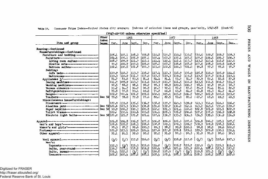
Table 12. Consumer Price Index—United States city averape: Indexes o f selected items and groups, quarterly, l?U7-58 (Cont'd)
(1947-49=100 unless otherwise specified)
Item and groupOtherindexbfigSP
1956 1957 1958!iar. June Sept. Dec. Mar. June Sept. Dec. Mar. June Sept.
106.1 107.1 108.3 109.8 110.2 110.7 110.2 110.5 110.0 109.5 109.7 109.310U .1 105.1 105.9 107.1 107.14 107.7 107.1 107.5 107.0 106.5 106.7 106.3108.7 109.9 111.3 112.1 111.14 112.1; 112.1 113.3 113.2 113 .li 112.8 112.5
99.0 100.9 103.C 106.0 107.2 107.7 108.6 107.9 107.6 108.2 109.6 108.9102.1 102.5 101.8 102.3 1C3.0 102.5 100.3 101.0 99.8 97.7 97.8 97.8110.9 112.2 113.7 116.2 117.14 117.3 116.9 116.0 115.8 116.0 115.9 IU4.8110.3 110.9 11)4.7 117.0 117.5 119.3 119.7 119.8 119.5 118.7 119.1 119.18U.7 83.6 83.6 814.1 814.1 814.14 83.7 Slu7 82.9 82.If 82.8 82.8
111.? 109.9 110.7 111.6 110.9 111.7 111.5 112.2 113.5 llli.5 116.7 1114.798.5 98.2 98.1 98.2 98.3 98.9 100.6 100.7 98.6 97.8 97.6 98.395.2 9U.7 96.9 96.8 90.2 92.6 87.8 87.6 85.9 86.U 85.1) 80.975.8 72*8 70.14 69.8 71.8 66.8 63.8 614.2 6 I4 . 8 65.3 6 I4 . 7 61.2
102.2 101.U 101.7 102.6 102.1 105.1 103.9 1014.5 120.7 102.9 102.6 103.278.5 78.0 77.9 77.6 80.8 82.5 83.0 82.2 67.2 68.0 69.5 69.5127.9 133.2 135.5 136.7 138.2 137.7 II4O. 3 139.9 Hi3.3 lltl.C II4 6 . I II4 6 .C121.6 123.3 130.0 131.8 131.6 132.2 136.0 II42.I 1143.2 1143.1 135.0 139.299.9 100.2 100.3 100.8 102 .C 101.3 101. k 102.0 102.8 •101.9 103.1 102.9
100. h lo o .U 100.6 103.5 10k.h 105.3 105.7 106.6 107.0 108.0 106.9 1 0 8 . 0121.2 121.7 121.8 121.1; 128.Ii 131.7 133.3 1314.3 1314.5 135.0 13U.9 1314.9IOI4 . 8 10U .8 106.5 107.0 106.8 106.6 107.3 107.6 106.8 106.7 107.1 107.5106.6 107.5 108.3 108.6 108.8 109.1 109.3 109.5 108.9 108.8 108.3 108.1498.3 97.5 99.6 100.3 99.3 98.5 99.8 100.1 98.8 98.5 99.6 100.2
121.9 123.1 126.0 126.14 127.6 127.8 128.1 129.1 129.5 129.8 130.1 130.1491.1 91.1 92.0 92.2 92.2 91.9 92.3 • 92.3 91.9 91.9 92.0 92.3
(h/) (h,f) 117.5 116.0 ( V ) (,h/ ) 118.9 117.0 (h/) (]*/) 118.6 117.3112.3 ( V ) 115.3 115.0 1114.2 ( V ) 115.7 115.7 112.0 (W ) 115.1 lllw3116.7 117.1 118.5 119.5 120.14 120.6 121.U 121.9 122.14 127.6 123.3 123.5HU.lt105.5
115.2 105. U
( V )107.2
( V )ioU . 1
116.8 108 .ii
118.0 108.14
<y>108.3( V )
IOB.1;119.8108.1
121.3108.5
(.k/) 109.7 ( V )109.0
Housing— ContinuedHousefurni ahings— Continued Furniture and bedding- Furniture-
Living room suite s- Dinette sets------Bedroom suites-
Bedding:Sofa beds----Mattresses----- ---- — ----
Appliances --- ---- --- --- —Sewing machines------- ------Washing machines— -----Vacuum cleaners— --- ----- --Refrigerators— — — — -------Toasters---------------------
Miscellaneous housefurnishings:Dinnerware-------------------Aluminum pans— — ------------Paper napkins— --------------Toilet tissue----------------Electric light bulbs---------
Apparel------------Hen's and boys'- Women's and girls'- Footwear-
Dee 52
Dec 52 Dec 52Dec 52
Other apparel-Wool apparel— -------Men's:Topcoats--- --- —Suits, year-round-Suits, summer----Trousers— ---- -
100 PRICES
AND W
AGES
IN M
AN
UFA
CTU
RIN
G
IND
UST
RIE
S
Digitized for FRASER http://fraser.stlouisfed.org/ Federal Reserve Bank of St. Louis
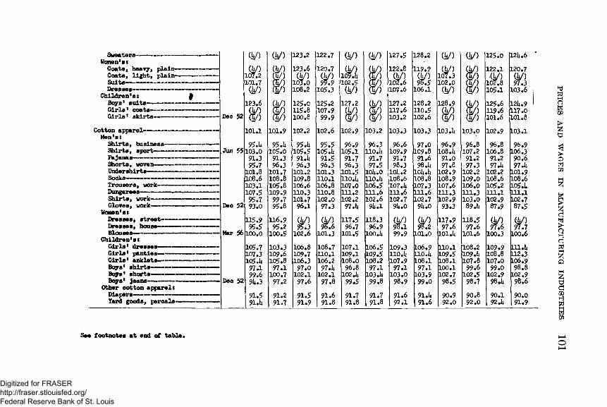
Sweaters—Women's*Coat8, heavy, plaiiCoats, light, plain--- —Suits------------------Dresses— — — — ---- ~
Children's s fBoys' suits Girls' coats- Girls* skirts*
Cotton apparel-— --Men's:
Shirts, business- Shirts, sport---Pajamas----Shorts, wove: Undershirts- Socks*Trousers, work*Dungarees-----Shirts, work— Gloves, work— -
Women's*Dresses, street— Dresses, house- Blouses-
Children's*Girls' dresses-Girls1 panties- Girls' anklets- Boys' shirts—
shorts- Boys' Jeans-
Other cotton apparelsDiapers-------- ---Yard goods, percale-
Dec 52
Jun 55
Dec 52
Mar 56
Dec 52
(V)
107.2101.7(V)
123.6 ;>
101.195 .U 103.0 91.395.7
101.8 108.6 103.1 107.595.793.0115.9
95.5 100.0105.7107.3 105.1*97.199.6 9l».391.591.U
(V) 123.2 122.7 (V) (V)(V)
¥
123.6(V)103.0
120.7(]i/)99.9
(V)109.14102.5
(U/)
m(1/) 108.2 105.3 (V) <!/>(V) 125.0 125.2 127.2 (V)i\
115.8100.8.
107.999.9
(V)(%/) 3 3
101.9 102.2 102.6 102.9 103.295 .U 95 .U 95.5 96.9 96.3ic5.0 105.5 105.14 105.1 110.lt91.3 91.14 91.5 91.7 91.796.3 96.3 96.3 96.3 97.5101.7 101.2 101.3 101.5 IOI4 .O108.8 109.8 110.1 110.U UO.I4105.8 106.6 106.8 107.0 106.5109.9 110.3 110.8 111.2 111.699.7 101.7 102.0 102.2 102.695.8 96.1 97.3 97.14 9U.1
116.9 (V) (V) 117.5 118.395.2 95.3 96.6 96.7 96.9
100.5 102.6 101.3 101.5 100.1*103.3 106.8 108.7 107.1 106.5109.6 109.7 110.1 109.1 109.5105.8 106.3 106.2 108.0 108.297.1 97.0 97.14 96.8 97.1100.7 102.1 102.1 102 .I4 103.1i97.2 97.6 97.8 99.5 99.891.2 91.5 91.6 91.7 91.791.7 91.9 91.8 91.8 91.8
127.5 122.8
107*6127.2117.6 103.2
103.396.6109.9 91.7 98.3
10U.2108.6107.U111.6102.7914.0
(V)95.199.9109.3 110.1*107.997.1
103.098.991.692.1
128.2119.9(V)96.5
106.1 .128.2110.5102.6
103.397.0
109.891.6 98.U
I0 I4 .I4108.8107.3 111.6 102.79U.0
(V)98.2
L01.0
L06.9110.1;108.197.1
P-03.999.091.1491.6
(V)(V)107.3
102.0(V)
128.9 (^ )
103.596.9
108 .I4 91.097.8102.9108.9107.6111.3102.9 93.3117.9 97.6
101.1*110.1109.5108.1100.1102.798.590.9 92.0
103.096.8
107.291.297.3
102.2109.0 106.0 111.3 103.089.14118.597.6
101.6108.2109.lt107.899.6
102.598.790.8 92.0
125.0122.1
(V)102.8105.1125.6119.6101.6102.996.8
106.8 91.2 97 .14
102.2 108.6 105.2 111.1102.9 87.9(V)97.6
100.3109.9 108.8 107.099.0
102.9 98.U90.1 92 .U
12U.6
120.797.3
103.6
12U.9117.0 101.8103.1
96.9lo6.390.6 97 .li
&.01.9 108.6 105.14111.1 102.787.5
97.7 100.6LII.I4L12.3106.998.8
[L02.998.690.091.9
See footnotes at end o f table.
PRICES AND
WAGES
IN M
AN
UFA
CTU
RIN
G
IND
USTR
IES
101
Digitized for FRASER http://fraser.stlouisfed.org/ Federal Reserve Bank of St. Louis
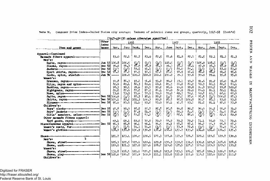
Table 12. Consumer Price Index—United States city average: Indexes of selected items and groups, quarterly, 19li7-58 (Cont'd)
(194.7-49=100 unless otherwise specified)________________
Oto
Item and groupOtherindexb&sea Mar.
1956June Sept. Dec. Mar* June Sent
1251-Dec. Mar * June Sept * Dec *
1956
Apparel— ContinuedManmade fibers apparel- Men*stSuits, rayon--Slack8, rayon--------- — -----Jackets-----------------------Sport shirts, rayon-----------Socks, nylon, stretch---------
Women1stDresses, rayon— — ------------Slips, rayon and nylon— — ----Panties, rayon--- — ---------Nightgowns, rayon— -- -------Hose, nylon-Suits, rayon—Skirts, rayon-Blouses— — --
Children’st Boys' slacks—Boys' Jackets-Girls' sweaters, orIon-------
Other manmade fibers apparel:Yard goods, rayon------------
Miscellaneous apparel------------Women'8 coats, fur— --- -— ----Women18 girdles-
Shoes- Men'stShoes, street-Shoea, work--
Women’st
Jun 53 Dec 52 Dec 52 Dec 52 Jim 56
Dec 52 Dec 52 Dec 52Dec 52 Dec 52 Dec 52
Dec 52
Shoes, street-Shoes, play-
Children'siDec 52
83.0100.896*6(V)97 .7
9 1 .8 80.698 .386.87 3 .6
100*6 101*1
9 5 .6
9 7 .8
69.h9 6 .3iU/)1315.9
121*7
1 2 5 .3120.0116.8105.6
82*1
100*596*3
(y>97*7
100.088*380*L|9 8 .1 87*6 7 3 .3 0 * /)99.2 93*6
98*0
69*195.8(J*/)
130*9
123.1*
1 2 7 .5121*3
118.1106.8
8 2 .7
(V)97*68 9 .5 97*5
100*2
93.k 80*3 99*6 87*87 1 .6 97 *3
101*391.1*
98*58P .989*5
6 9 .6 96.14 7 iu l
1 3 0 .9
1 2 6 .0
1 2 9 .11 2 7 .0
121.11 0 8 .9
8 3 .0
(V) 9!? .99 1 .1 9 7 .5
100*09U.680*1-99*588*272*595.1;
1 00 .393*0
9 5 .781**989*270.096.1471**0
130*9
126*5
129.1*1 2 7 .6
121*71 0 9 .9
8 2 .5
(V)9 5 .3(V)97*7
100.19 3 .280. h 99*288 .U7 0 .9 99*299.9 9 3 .0
9 5 .8
W ?(5/)
70*09 6 .5(V)
137 .2
1 27 .3
129*9128*2
122*9111*1
81*6
102*596*3<y>.97*5
100.090*281*398*686*070*0(V)9^ .792.1*
9 5 .8(V)(g n
6 8 .9 96*1 ( V )
1 3 2 .2
127*6
130*3129*0123.2111*0
81*8
(h/)9l.$89.09 7 .69 9 .3
9 3 .1 80*2 99*0 86.0 69*398.2 98.8 91.896.886*085.U70.297*77 3 .9
1 3 3 .7
127*9
130*8128*5
1 2 3 .5111*9
82*1
(V)9 8 .1 88.1, 98*69 9 .6
9 3 .280.29 9 .8 86*0 70*1;9 7 .6
100.893*2
96.8 81**5 85.07 0 .297*172*6
133*7
128*5
131*5128*5
1214*5
81*5
1 0 5 .997*9(V)98*29 9 .0
91*68 0 .399.986*069*897*895*791.896*0
887 1 .1 96*2 (V)
13U .0
129*1
1 3 0 .11 2 9 .3
1 2 5 .8
82.1
1 0 8 .5 9 8 .3(V)96.299.1*
9 1 .28 0 .3
10 0 .5 86.16 9 .3 (1*/) 9Z.3 91.ii
96*2
70*096*3(V)
13U.0
129*5
1 2 9 .5 1 2 9 .9
126*3111.6 j110.7 112.6
81*3
(V)91.983*09U.29 5 .8
9 5 .0 80.2 99*8 86*1 68*14
100*593*092*5
96*08i*.582.67 0 .79 6 .771.0
13)4.5
1 2 9 .7
128.61 2 9 .5
1 2 6 .71 1 2 .7
8 1 .3
(V)9 6 .88 3 .09 5 .19 5 .0
91*.8 80.1*
100.286.16 8 .99 7 .39 3 .29 3 .9
91*.2 88.68 0 .9
70*697*27 1 .3
1 3 5 .3
130*0
128*5130*2128*0113*2
PRICES AND
WAGES
IN M
ANUFACTURING IN
DU
STRIES
Digitized for FRASER http://fraser.stlouisfed.org/ Federal Reserve Bank of St. Louis
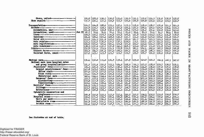
Shoes, oxford— --------------— -- 126.6 128.3 130.3 130.5 131.0 130.9 131.1 132.0 ‘131* .3 134.6 135.8 135.2Shoe repairs— — ------ -— 115.7 116.1 117.3 119.2 123.7 125.6 126.8 129.8 130.0 132.0 133.5 133.7
Transportation-— — -— -— --------- --- 126.7 126.8 128.6 133.1 135.1 135.3 135.9 138.9 138.7 138.9 11*1.3 144.3Private---- - 116.8 116.7 118.7 123.3 125.2 125.U 125.5 128.6 128.0 128.0 130.1* 133.3Automobiles, new— — — — — -— ---- 121.8 120.1 118.5 132.6 130.1 128.1 125.0 135.2 132.1* 130.8 130.1 143.6Automobiles, used— ------ — — Jan 53 68.7 70.1* 71* .1* 76.1 79.1 81.0 83.1* 82.3 79.1* 81.7 88.1* 89.6Tires™-- — -— -----------— — — 129.5 122.1 129.7 130.9 127.5 125.1* 131.8 133.6 133.2 131.1 131*.8 138.8Gasoline— — — ------ --------- 124.4 125.6 129.6 128.8 132.9 132.7 131.2 131.5 129.5 129.2 131.9 126.7Motor oil— — — — ----- --------- 113.9 114.3 111*. 9 118.2 123.7 125.0 121*.7 125.1 126.3 126.3 125.9 126.4Auto repairs---- — — — ------------- 133.3 131* .2 135.9 137.5 138.1 139.6 11*0.1* 11*2.1* 11*1.3 11*1.6 11*2.1 142.6Auto registration— ------------— - 120.5 121.0 121.1* 121.1* 123.5 123.6 123.7 123.6 126.3 127.5 127.6 127.6Auto insurance— ------------------ 138.3 137.9 137.7 137.8 11*6.3 11*8.5 153.0 155.9 171.8 171.8 173.2 173.0
Public------ '----------------------- 170.8 172.6 173.0 171*. 1 175.8 176.8 181.1 182.1* 185.9 187.7 189.8 191.8Transit fares----- — -------------- 183.9 181*.0 18)* .6 186.0 186.0 187.5 193.2 191*. 8 198.3 200.7 203.5 205.0Railroad fares, coach--- — — — — 117.5 123.7 123.7 123.7 129.7 129.7 129.7 129.7 132.9 132.9 132.9 136.1
^ ________________________ 131.1* 132.0 131* .0 131*. 7 136.1* 137.9 139.0 11*0.8 11*2.3 144.2 146.5 147.6Medical care less hospital ratesand group hospitalization— — — — 121.2 121.6 122.5 123.1 124.9 125.9 126.3 127.7 128.9 129.7 130.2 131.1Physicians * fees----- --- ----- --- 126.3 126.9 127.9 128.0 132.3 132.5 *132.8 135.8 136.0 137.0 137.5 138.6General practitioners * fees------ 127.8 128.3 129.3 129.1* 131* .1* 131* .1* 13U .6 136.9 138.3 139.1* 139.9 141.1Office visit------------------ 127.0 127.2 127.5 127.5 131.2 131.1* 131.7 133.3 131*. 9 136.5 137.1 138.3House visit------------------- 12U.U 124.9 126.5 126.5 133.5 132.9 133.1 136.3 137.5- 138.3 138.3 139.6Obstetrical care— — — — 142.1* 11*1* .1 11*6.6 11*7.0 1148.1* 150.2 150.1* 151.6 152.8 152.8 155.1 156.0Surgeons• fees-------- ------ --- 117.3 118.1 118.7 119.6 119.9 120.9 121.6 121.9 122.3 122.6 122.9 123.5Appendectomy-- — ------ — — — 116.6 117.8 118.1 119.1 119.6 119.6 119.8 119.3 120.0 120.0 120.2 120.7Tonsillectomy— -- — --- — --- 119.li 119.1* 120.ii 121.2 121.0 121* .2 125.7 127.8 127.3 128.1* 128.7 129.7Dentists' fees— --- — ----- — ----- 121*.1* 121*.3 121* .5 125.1* 126.6 127.1* 128.0 128.6 130.2 131.3 132.5 133.3Fillings--------*--------------- 123.7 123.1* 123.7 121*.6 125.7 126.7 127.2 127.8 129.6 130.6 132.0 132.7Extractions------ ------- ------- 127.8 128.8 128.3 129.6 131.0 131.5 132.1 132.9 133.5 135.3 135.6 136.9Optoraetric examination andeyeglasses--— -— -— — --- — 109.9 110.9 112.1 112.9 115.1* 116.2 115.5 116.1 116.5 116.8 116.8 116.7Hospital rates-— - — — — — --- 169.6 171.2 176.7 180.1 183.6 185.1* 191.0 193.5 196,1* 197.6 199.3 201.1Men's pay ward----- 179.7 181.0 186.5 193.3 198.0 199.6 206.3 211.4 21U.5 215.1 216.1* 219.0Send private room-— — — — — --- 165.8 168.2 171* .it 176.1 179.3 180.9 187.2 188.9 191.8 193.2 194.9 196.5Private rocn— — ----------- 161.6 162.8 167.2 168.8 171.3 173.1 177.3 177.9 180.6 182.2 184.1 185.3
See footnotes at end of table.
PRICES AND
WAGES
IN M
AN
UFA
CTU
RIN
G
IND
USTR
IES
103
Digitized for FRASER http://fraser.stlouisfed.org/ Federal Reserve Bank of St. Louis
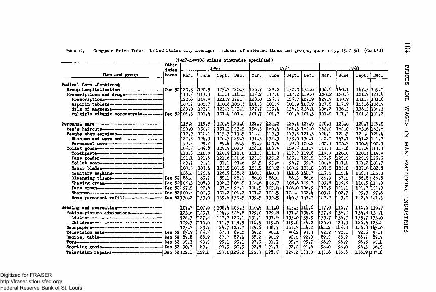
Table 12. Consumer Price Index—United States city average: Indexes o f selected items and groups, quarterly, 12U7-58 (Cont*d)
(1947-49=100 unless otherwise specified)
Item and groupTJtKSr'indexbases
1956 1957 1958Mar. June Sept* Dec. Mar. June Sept. Dec. Mar. June Sept. Dec.
Medical Care— ContinuedGroup hospitalization------ — ------- Dec 52 120.3 120.9 125.7 126.3 126.7 129.2 132.0 13ii.6 136.8 liiO .l Iii7.5 Iu9.1Prescriptions and drugs— ------------ 113.5 113.3 l l i l . l IU4J4 115.2 117.0 117.2 119.0 120.2 120.3 121.2 121 J*Prescriptions--’----— -------------- 120.6 119.9 121.9 122.3 123.0 125.3 125.7 127.9 129.9 130.9 131.3 131.8Aspirin tablets— — ----- ------- ----- 100.7 100.7 100.8 100.3 101.3 101.9 101.9 105.9 107.5 107.9 103.6 108.9Milk of magnesia— ---------------- 123.0 123.1 123.1 123. ii 127.7 135 .li 136.1 136.1 136.2 136.3 136.3 136.3Multiple vitamin concentrate------- Dec 52 101.3 101.ii 101J4 101.ii 101.7 101.7 101.6 101.3 101.0 101.2 101.2 101.2
Personal care— - - — ----------------- 119.2 119.9 120.5 121.8 122.9 L2i|.2 125.1 127.0 128.3 128.6 123.7 129.0Men's haircuts— -- ------------- — 150.0 150.0 151.1 153.5 156.3 l60.ii 161.3 162.0 162.0 162.0 163.6 163.6Beauty shop services— — — — ----- - 112.9 liii.i 115.3 117.5 118. >4 119.3 119.3 121.3 12U.1 12ii.5 12ii.)| 12U.U
122.3 12iw3 126.3 129.7 131.3 132.3 133.0 136.1 l!;0.7 liil.l iia.2 11*1.2Permanent wave— — ----------------- 99.3 99.2 . 99.ii 99.9 99.9 100.5 99.8 100.2 100.3 100.7 100.il 100.3
Toilet goods---- — --- — — --------- - 105.5 105.8 105.9 107.0 108.1 108.9 109.5 111.7 113.3 113.8 113.5 113.3Toothpaste---- ---- ------------ -- 110.3 110.9 110.5 111.0 111.3 111.3 112.2 119.8 119.9 120.0 120.1 119.9Face powder— -— — ----------- — 121.1 121.6 121.6 12U.6 125.2 125.2 125.i4 125.5 125.5 125.5 125.5 125.5Toilet soap— — — — — —— 89.7 90.1 91.1 91.6 92.5 95.6 96.7 99.7 100.6 101.ii 101.2 101.7Razor blades— — — — ---------- 103.3 103 .ii 103.2 103.2 103.2 103.2 103.2 103.0 103.0 103.0 103.0 102.3Sanitary napkins------------------- 1 2 6 .1 4 1 2 6 . h 126.5 1 3 6 . 8 liiO.3 liiO.3 H 4I .6 liiii.7 lii5.ii lii6 .ii 1U6.3 H1 6 .OCleansing tissue--- --------------- Dec 52 8 6 .ii 85.7 85.1 8 6 . 1 86.0 8 6 . 0 86.3 8 6 . 6 8 6 . 9 87.0 8 6 . 8 86.3Shaving cream— -- — -- — — -- — Dec 52 108.5 108.3 108.3 108.5 108.6 108.7 1 0 8 . 6 109.7 109.8 109.9 110.5 110.3Face cream-— — ---- — -- -- --- Dec 52 97.5 97.6 97.6 98.1 10ii.5 105J4' 1 0 6 . 0 106.9 117.5 1 2 1 . 1 121.7 121.9Shampoo— — — -- — — — --- Dec 52 1 0 0 . 8 100.3 1 0 1 . 2 1 0 1 . 2 1 0 1 . 2 102.5 1 0 2 .ii 1 0 2 . )4 103.1 102.7 99.3 97.6Home permanent refill— — — — ---- Dec 52 1 3 6 . 2 139.0 139.6-139.5 139.5 139.5 lii0.5 Uil.7 1U2.2 li43.0 li |2 . 6 liil.5
Reading and recreation------- — — — -- 107.7 1 0 7 . 6 IO8J4 109.3 110.5 111.8 113.3 III4.6 117.0 116.7 116.6 116.9Motion-picture admissions— — — — 1 2 3 . 6 125.1 12ii.9 126.8 129.0 129.8 131.2 13li.5 137.8 1 3 6 . 0 131*.8 13i*.l
126.3 127.8 127.2 129.1 131.1 131 .ii 133.0 135.9 139.7 136.7 135.7 135.0Chi ldren— — — --------- --- ------- 109.3 1 1 0 . 6 111.9 113.9 116.5 119.0 1 1 9 . 8 1 2 ii. 2 126.0 128.3 126Ji 1 2 5 . 8
Newspapers-— ---- — -— — — ---- — ----- 123.7 123.7 12i4.7 12U.7 1 2 5 . 6 138.7 liil.7 liiii. 2 liiii. 2 li45.3 li*l* . 8 lii5 . 0Television sets— — — — — — -- — Dec 52 85.9 85.5 87.3 89.0 89.2 90.1 90.2 93.3 92.2 90.1 92.6 93.1Radios, table— --- ---- — ------ --- Dec 52 89.8 88.9 87.7 87.ii 88.2 90.9 92.0 92.3 89.2 83.2 86.7 87.7Toys------------------------ ------- Dec 52 95.3 93.5 95.1 95.1 97.5 91.7 1 95.6 95.7 96.9 96.9 96.8 95.1iSporting goods— ------------------ Dec 52 90.7 89.U 90.5 90.5 92.8 91.1 1 92.0 91.6 98.0 98.0 96.5 96.5Television repairs— — — — - ■ Dec 52 122.1 122.ii 123.1 125.2 126.3 128.5 129.2 133.3 133.6 1 3 6 . 8 136.9 137.8
104 PRICES
AND W
AGES
IN M
AN
UFA
CTU
RIN
G
IND
UST
RIE
S
Digitized for FRASER http://fraser.stlouisfed.org/ Federal Reserve Bank of St. Louis
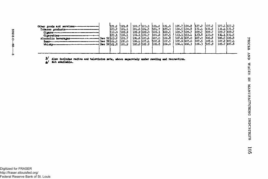
50505 0
—60----------8
Other goods and services-Tobacco products-
Cigars-Cigarettes-
Alcoholic beverages- Beer-Whisky-
121*2 121.8 122.7 123.3 12U.2 12U.6 126.7 126.8 127.2 127.2 127.1 127.3123.2 12li.l 12li.6 12J4.5 12iw7 125.3 130.5 130.8 131.1 131.2 i3i.a 131.7L10.0 109.9 109.9 109.0 109.3 109.5 109.7 109.7 109.7 109.7 109.7 109.7L25.1 126.1 126.6 126.7 126.8 127.5 133.1 133 .a 133.8 133.9 i3a.i ua.5
Dec 52 L03.2 103.7 10U.6 105.6 107.0 106.8 107.1 107.0 107.0 106.8 106.5 106.8Dec 52 L0l*.2 105.0 106.U 107 .h 107.8 107.5 107.6 107.6 107.5 107.a 107.2 107 .aDec 52 L01.8 101.9 102.0 102.9 105.8 106.0 106.U106.3 106.3 105.9 105.7 105.8
2 / Also includes radios and television sets, shown separately under reading and recreation# i/ Hot aTtllaU *.
PRICES AND
WAG
ES IN
MA
NU
FAC
TUR
ING
IN
DU
STRIE
S 105
Digitized for FRASER http://fraser.stlouisfed.org/ Federal Reserve Bank of St. Louis
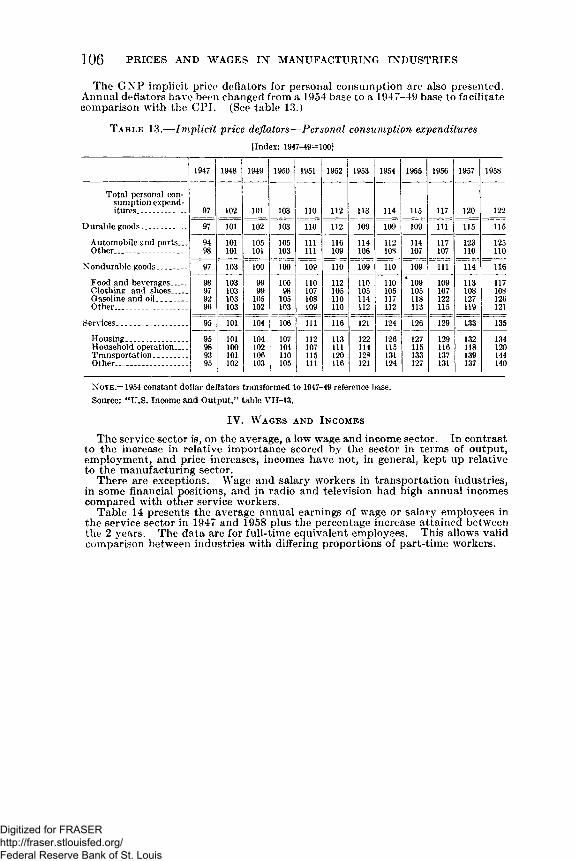
The GNP implicit price deflators for personal consumption are also presented. Annual deflators have been changed from a 1954 base to a 1947-49 base to facilitate comparison with the CPI. (See table 13.)
T a b l e 13.— Implicit price deflators— Personal consumption expenditures
106 PRICES AND W AG ES IN M ANUFACTURING INDUSTRIES
| Index: 1947-49=100]
1947 1948 1949 1950 1951 1952 1953 1954 1955 1956 1957 1958
Total personal consumption expenditures____________ 97 1 0 2 101 103 11 0 1 1 2 113 114 115 117 1 2 0 1 22
Durable g o o d s ................ 97 101 10 2 103 11 0 11 2 109 109 109 111 115 115
Automobile and parts... 94 101 105 105 111 116 114 112 114 117 123 125Other......... ........... .......... 98 101 101 103 111 109 106 108 107 107 1 1 0 1 1 0
Nondurable goods.......... . 97 103 1 0 0 100 109 11 0 109 1 10 109 111 114 116
Food and beverages____ 98 103 99 100 11 0 112 110 11 0 * 109 109 113 117Clothing and shoes 97 103 99 98 107 105 105 105 105 107 108 108Gasoline and oil_______ 92 103 105 105 108 11 0 114 117 118 122 127 126Other_____________ ____ 96 103 10 2 103 109 11 0 112 112 113 115 119 121
Services..................- ............ 95 101 104 106 111 116 121 124 126 129 133 135
Housing_______________ 95 101 104 107 112 113 122 126 127 129 132 134Household operation___ 98 1 0 0 102 1 01 107 111 114 115 115 116 118 1 20Transportation................ 93 101 106 110 115 120 128 131 133 137 139 144Other_________________ 95 102 103 105 111 116 121 124 127 131 137 140
N ote.—1954 constant dollar deflators transformed to 1947-49 reference base.Source: “ U.S. Income and Output,” table VII-13.
IV. W a g e s a n d I n c o m e s
The service sector is, on the average, a low wage and income sector. In contrast to the increase in relative importance scored bv the sector in terms of output, employment, and price increases, incomes have not, in general, kept up relative to the manufacturing sector.
There are exceptions. Wage and salary workers in transportation industries, in some financial positions, and in radio and television had high annual incomes compared with other service workers.
Table 14 presents the average annual earnings of wage or salary employees in the service sector in 1947 and 1958 plus the percentage increase attained between the 2 years. The data are for full-time equivalent employees. This allows valid comparison between industries with differing proportions of part-time workers.
Digitized for FRASER http://fraser.stlouisfed.org/ Federal Reserve Bank of St. Louis
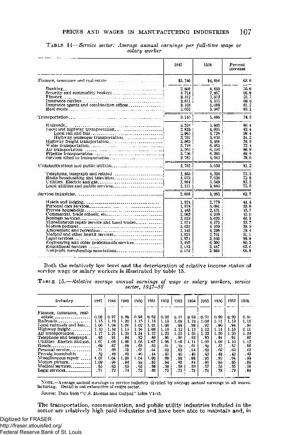
PRICES AND W AGES IN M ANUFACTURING INDUSTRIES 107
Table 14— Service sector: Average annual earnings per full-time wage orsalary worker
1947 1958 Percentincrease
Finance, insurance and real estate________ ________ _________ $2,740 $4,484 63.6
Banking___________ _____________________________________ 2,860 4,433 55.0Security and commodity brokers_________________________ 4, 714 7, 867 66.9Finance______ ____ - . . ____ _____________________________ 3,412 5,313 55.7Insurance carriers________________________________________ 2,811 4, 515 60.6Insurance agents and combination offices________________ 3,103 5, 018 61.7Real estate__________ _____ _____________________________ 2,052 3,347 63.1
Transportation __________ __________ ________ ____ ________ 3,145 5, 488 74.5
Railroads_____________________ __________________________ 3,216 5,803 80.4Local and highway transportation_____ _________________ 2,833 4,035 42.4
Local rail and bus. _________ _______________________ 2,965 4, 726 59.4Highway passenger transportation______ ____________ 2,707 3,634 34.2
Highway freight transportation______________ ______ _____ 3,063 5,468 78.5Water transportation____________________ _____ _________ 3,748 6,463 72.4Air transportation___ ________________________ ___________ 3,265 6,104 86.9Pipeline transportation_____ ___ _____ ______ ___________ 3, 750 6,360 69.6Services allied to transportation..._____ _________________ 2.762 4,944 79.0
Communications and public utilities______1 . . . ............ .............. 2,792 5,059 81.2
Telephone, telegraph and related________________________ 2,583 4,528 75.3Radio broadcasting and television_______________________ 4,073 7,038 72.8Utilities: Electric and gas------------------------------------------------- 2,994 5,549 85.3Local utilities and public services_______ _______________ 2,217 3,880 75.0
Services industries_____________________________________ ______ 2,005 3,262 62.7
Hotels and lodging................... ............. ............ ................ ....... 1,924 2,779 44.4Personal care services................................... ............................. 1,978 3,081 55.8Private households. ____ ________ _____________________ 1,463 2,131 45.7Commercial, trade schools, etc......... ........................ .............. 2,903 4,209 45.0Business services________________________________________ 3,023 5,022 6 6 .1Miscellaneous repair service and hand trades____________ 2.974 4, 572 53.7Motion pictures______________________________________ .. 3,031 4,209 38.9Amusement and recreation. ____ ______________________ 2,345 4,206 79.4Medical and other health services_________ ______________ 1,821 2, 751 51.1Legal services____ . . __________ ______ ________________ 1,971 3,940 99.9Engineering and other professionals services_____________ 3, 495 6,302 80.3Educational services ______ ____________________________ 2,113 3,457 63.6Nonprofit membership associations______________________ 2,172 3,669 6 8 . 9
Both the relatively low level and the deterioration of relative income status of service wage or salary workers is illustrated by table 15.
T a b l e 15.— Relative average annual earnings of wage or salary workers, servicesector, 1947-58
Industry 1947 1948 1949 1950 1951 1952 1953 1954 1955 1956 1957 1958
Finance, insurance, real- estate.__............................ 0.98 0.97 0.98 0.98 0.93 0.92 0.91 0.93 0.91 0.90 0.90 0.91
Railroads.............................. 1.15 1.19 1 .2 0 1.15 1.16 1.13 1.09 1 .1 0 1.08 1 .1 1 1.13 1.18Local railroads and bus... 1.06 1.04 1.06 1 .0 2 1 .0 1 1 .0 0 .98 .99 .97 .96 .94 .96Highway freight_________ 1 .1 0 1 .1 0 1.15 1.16 1.09 1 .1 0 1 .1 2 1.13 1 .1 2 1 .1 1 1 .1 0 1 .1 1Air transportation_______ 1.17 1 .2 1 1.25 1.24 1 .2 2 1.23 1 .2 2 1.25 1.23 1 .2 0 1 .2 0 1.24Telephone and telegraph . .93 .91 .94 .92 .89 .90 .90 .93 .93 .91 .91 .92Utilities: Electric and gas. 1.07 1.06 1.09 1.08 1.07 1.08 1.09 1 .1 1 1.09 1.09 1 .1 0 1 .1 2Hotels___________________ .69 .67 . 6 8 . 65 .62 .61 .59 .61 .59 .57 .57 .56Personal service..... ............ .71 .69 .70 .67 .64 .63 .63 .64 .63 .62 .62 .62Private households______ .52 .49 .49 .46 .44 .45 .46 .46 .43 .43 .43 .43Miscellaneous repair.......... 1.07 1.04 1.05 1.04 1 .0 0 .99 .98 .98 .95 .95 .94 .93Motion picture................... 1.09 .96 .94 . 8 8 .85 .84 .81 .84 . 8 6 .85 .85 .85Medical services............. . .65 .63 .65 .63 .59 .59 .58 .59 .57 .55 .55 .56Legal services.......... .......... .71 .72 .74 .72 .69 .72 .73 .75 .76 .78 .79 .80
N o t e .— Average annual earnings in service industry divided by average annual earnings in all manufacturing. Detail is not exhaustive of entire sector.
Source: Data from “ U.S. Income and Output” table VI-15.
The transportation, communication, and public utility industries included in the sector are relatively high paid industries and have been able to maintain and, in
Digitized for FRASER http://fraser.stlouisfed.org/ Federal Reserve Bank of St. Louis
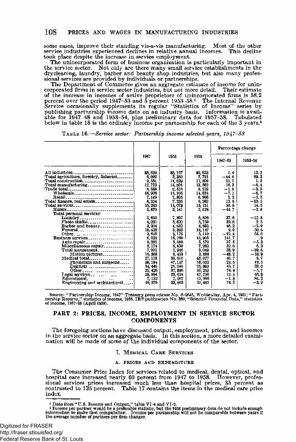
108 PRICES AND WAGES IN MANUFACTURING INDUSTRIES
some cases, improve their standing vis-a-vis manufacturing. Most of the other service industries experienced declines in relative annual incomes. This decline took place despite the increase in service employment.
The unincorporated form of business organization is particularly important in the service sector. Not only are there many small service establishments in the drycleaning, laundry, barber and beauty shop industries, but also many professional services are provided by individuals or partnerships.
The Department of Commerce gives an aggregate estimate of income for unincorporated firms in service sector industries, but not more detail. Their estimate of the increase in incomes of active proprietors of unincorporated firms is 58.2 percent over the period 1947-53 and 5 percent 1953-58.8 The Internal Revenue Service occasionally supplements its regular “ Statistics of Income” series by publishing partnership income data on an industry basis. Information is available for 1947-48 and 1953-54, plus preliminary data for 1957-58. Tabulated below in table 16 is the ordinary income per partnership for each of the 3 years.9
T a b l e 16.— Service sector: Partnership income selected years, 1947—58
Percentage change
1947 1953 1958 1947-53 1953-58
All industries----------------------------- --------------- $8,639 $8,757 $9,823 1.4 12.2Total agriculture, forestry, fisheries_______ 6,092 3,380 5,721 -44.6 69.3Total construction------------ ---------- ------------- 9,551 11,629 11,809 21.7 1.5Total manufacturing................... ............. . 12,722 14,801 13,562 16.3 -8.4Trade total------ ---------------------------------------- 8,688 8,518 8,219 -1.9 -3.5
Wholesale...--------------------------------------- 16,906 15,705 14,654 -7.1 -6.7Retail------------------- ------- ---------------------- 7.149 7,305 6,906 2.2 -5.5
Total finance, real estate__________________ 6,354 7,235 6,262 13.9 -13.5Total services---------------------------------------- 10,285 14,073 16,121 36.8 14.5
Hotels------------------------------ ------------------ 5,675 3,141 3,028 -44.7 -3.6Total personal services:
Laundry------- ---------- --------------------- 5,6954,021
7,807 6,806 37.6 -12.8Photo studio____ _________________ 5,620 5,759 39.8 2.5Barber and beauty.. . . _________ 3,304 4,832 4,693 46.2 -2.9Funeral______ ___________________ 10,428 9,393 14,147 -9.9 50.6Other____________________________ 3,625 3,176 5,119 -12.4 64.6
Business services____________ ______ 6,522 15,766 15,905 141.7 .9Auto repair.................................. ....... 4,282 5,888 5,579 37.5 -5.3Miscellaneous repair......................... 5,174 6,8305,046 7,262 32.0 6.3Total amusement_________________ 7,991 3,049 36.9 -39.6
Motion pictures____ __________ 16,308 8,453 3,898 -48.2 -53.9Medical total............................. ......... 27,178 38,184 39,610 43,077 45.7 8.7
Physicians and surgeons........... 47,157 53,033 23.5 12.5Dentists____________________ _ 14,446 21,046 25,893 45.7 23.0Other______ ______ _____ _____ 21,426 37,386 35,263 74.4 -5.7
Legal services_____ _____ _________ 28,994 32,624 47,736 12.5 46.3Educational___________ ___________ 7,132 7,007 12,906 - 1 . 8 84.2Engineering and architectural____ 19,370 33,803 32,482 74.5 -3.9
Source: “ Partnership Income, 1947” Treasury press release No. S-2645, Wednesday, Apr. 4,1951; “ Partnership Returns,” statistics of income, 1955. IRS publication No. 369; “ Selected Financial Data,” statistics of income, 1957-58 (April 1959).
PART 2: PRICES, INCOME, EMPLOYMENT IN SERVICE SECTORCOMPONENTS
The foregoing sections have discussed output, employment, prices, and incomes in the service sector on an aggregate basis. In this section, a more detailed examination will be made of some of the individual components of the sector.
I. M e d ic a l C a r e S e r v ic e s
a . p r ic e s a n d e x p e n d it u r e
The Consumer Price Index for services related to medical, dental, optical, and hospital care increased nearly 60 percent from 1947 to 1958. However, professional services prices increased much less than hospital prices, 35 percent as contrasted to 125 percent. Table 17 contains the items in the medical care price index.
s Data from “ U.S. Income and Output,” table VI-4 and VI-2.9 Income per partner would be a preferable statistic, but the 1958 preliminary data do not include enough
information to make that computation. Income per partnership will not be comparable between years if the average number of partners per firm changes.
Digitized for FRASER http://fraser.stlouisfed.org/ Federal Reserve Bank of St. Louis
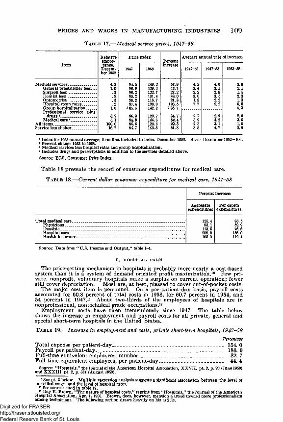
PRICES AND WAGES IN MANUFACTURING INDUSTRIES 109T a b l e 17.— Medical service prices, 1947-58
Relativeimpor
Price indexPercent
Average annual rate of increase
Item tance, December 1952
1947 1958increase
1947-58 1947-53 1953-58
Medical services ........................ 4.2 94.5 149.2 57.9 4.2 4.6 3.8General practitioner fees. __ 1 .6 96.9 139.3 43.7 3.4 3.1 2 . 1Surgeon fees........................... .3 96.2 122.7 27.2 2 . 2 2 . 8 1.5Dentist fees............................ . 8 95.2 131.4 38.0 3.0 3.5 2.3Optometrist..... ..................... .3 96.2 116.7 21.3 1 . 8 2 . 2 1.3Hospital room rates.............Group hospitalization..........Professional service plus
. 21 . 0
87.4 1 85.6
198.0142.2
126.5 2 35.7
7.7 9.2 6 . 06.3
drugs3.................................. 3.9 96.3 129.7 34.7 2.7 2.9 2 . 6Medical care ..................... 5.1 94.9 144.6 52.4 3.9 4.2 3.6
All items........................................ 1 0 0 .0 95.5 123.5 29.3 2.3 3.1 1.5Service less shelter....................... 16.7 94.7 143.8 51.8 3.8 4.7 2 . 8
i Index for 1953 annual average; item first included in index December 1950. Base: December 1952=100.3 Percent change 1953 to 1958.3 Medical services less hospital rates and group hospitalization.4 Includes drugs and prescriptions in addition to the services detailed above.Source: BLS, Consumer Price Index.
Table 18 presents the record of consumer expenditures for medical care.
T a b l e 18.— Current dollar consumer expenditure for medical care, 1947-58
Percent increase
Aggregateexpenditures
Per capita expenditures
Total medical care .......... .................... .......................................... ......... ................ 125.4 86.5Physicians. .......................................................................................................... 93.1 59.9Dentists_______________________________________________________________ 113.5 76.8Hospital care_________________________________ ________ ________________ 209.2 156.0Health insurance_______________________________________________________ 165.0 119.4
Source: Data from “ U.S. Income and Output,” table 1-4.
B . HOSPITAL CARE
The price-setting mechanism in hospitals is probably more nearly a cost-based system than it is a system of demand oriented profit maximization.10 Few private, nonprofit, voluntary hospitals make a surplus on current operation; fewer still cover depreciation. Most are, at best, pleased to cover out-of-pocket costs.
The major cost item is personnel. On a per-patient-day basis, payroll costs accounted for 60.8 percent of total costs in 1958, for 60.7 percent in 1954, and 54 percent in 1947.11 About two-thirds of the employees of hospitals are in nonprofessional, nontechnical grade occupations.12
Employment costs have risen tremendously since 1947. The table below shows the increase in employment and payroll costs for all private, general and special short-term hospitals in the United States.T a b l e 19.— Increase in employment and costs, private short-term hospitals, 1947-58
PercentageTotal expense per patient-day__________________________________________ 154. 0Payroll per patient-day_________________________________________________ 186. 0Full-time equivalent employees, number________________________________ 82. 7Full-time equivalent employees, per patient-day________________________ 44. 4
Source: “ Hospitals,” the Journal of the American Hospital Association, X X V II, pt. 2 , p. 23 (June 1953) and X X X III , pt. 2, p. 384 (August 1959).
10 See pt. 3 below. Multiple regression analysis suggests a significant association between the level of unskilled wages and the level of hospital rates.
11 See sources cited in table 19.12 Ray E. Brown, “ The nature of hospital costs,” reprint from “ Hospitals,” the Journal of the American
Hospital Association, Apr. 1,1956. Brown, does, however, mention a trend toward more professionalism among technicians. The following section draws heavily on his article.
Digitized for FRASER http://fraser.stlouisfed.org/ Federal Reserve Bank of St. Louis
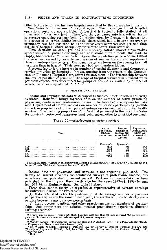
Other factors tending to increase hospital costs cited by Brown are also important.One factor is the nature of hospital costs. The major portion of hospital
operations costs are not variable. A hospital is typically fully staffed, at all times ready for a peak load. Therefore, the occupancy rate is a critical factor in average operating cost per bed. In studies cited by Brown, it is shown that in a group of otherwise similar hospitals, those which had a better-t.han-average occupancy rate had less than half the unrecovered overhead cost per bed than did those hospitals whose occupancy rates were lower than average.
While desirable on other grounds, the tendency tow’ard shorter stays makes syncronization of patient discharge and admissions more difficult; this leads to empty, nonrevenue-producing beds. Again, the population pattern of the United States is best served by an extensive system of smaller hospitals to supplement those in metropolitan centers. Occupancy rates are lower on the average in small hospitals than in large.13 Their costs per bed are therefore higher.
A second factor is the increase in number of special diagnostic and therapeutic services provided by hospitals. Brown, quoting from the report of the Commission on Financing Hospital Care, offers this statement, “ The relationship between the level of per diem expense and the scope of hospital service was apparent when per diem expense was determined for groups of hospitals classified by number of selected services they offered. * * *” 14
C. PROFESSIONAL SERVICES
Income and employment data with respect to medical practitioners is not easily available. Roberts 15 brings together data on the number of active practicing physicians, dentists, and professional nurses. The table below compares his data with Department of Commerce data on number of persons participating (including active proprietors of unincorporated enterprises) in medical and other health services. The declining proportion of professional personnel in the total illustrates the growing importance of nonprofessional technical and other lesser skilled personnel.
110 PRICES AND WAGES IN MANUFACTURING INDUSTRIES
T a b l e 20.— Employment in medical services
Year
Active physicians,
dentists, and nurses
Persons engaged in
medical and other health
services
Physicians, dentists, and
nurses as a percent of
total
1930 . ...........................................................................Thousands
439.2Thousands
749 58.61940....____ ______________________ _________________ _______ _ 529.3 841 62.91950______________________________ _________________ ________ 667.8 1,237
1,413 1,551
54.01953.................... .......... . . . ....................................................... ............ 706.2 50.01955....... ...................... .............................. ............................ .......... 745.6 48.0
Sources: Roberts, “ Trends in the Supply and Demand of Medical Care,” table 8 , p. 70; “ U.S. Income and Output," table VI-16 and “ National Income,” table 28.
Income data for physicians and dentists is not regularly published. The Survey of Current Business has conducted surveys of professional income, but none have been published for recent years.16 Partnership income data has been published by the Internal Revenue Service for the years 1947-48, 1953-54, and for 1957-58, preliminary data. See table 16 above.
These data cannot safely be regarded as representative of average earnings for individual doctors for two reasons:
(1) Data tabulated is for the partnership; if the average number of partners per partnership is not the same in each year, the results will not be strictly comparable between years on a per person basis.
(2) Many doctors, dentists, and other practioners are not members of partnerships. Sole proprietors and salaried medical practitioners experience different earnings records.17
i* Brown, op. cit. says, “ During 1954 those hospitals with less than 25 beds averaged 51.6 percent occupancy while those with over 300 beds averaged 71.8 percent occupancy.”
15 Markly Roberts, “ Trends in the Supply and Demand of Medical Care,” Study Paper 5 in the “ Study of Employment, Growth and Price Levels” (1959).
w See William Weinfeld “ Income of Dentists, 1929-48” Survey of Current Business, January 1950; “ Income of Physicians, 1929-49,” ibid, July 1951; “Income of Lawyers in the Postwar Period,” ibid, December 1956.
n Ibid.
Digitized for FRASER http://fraser.stlouisfed.org/ Federal Reserve Bank of St. Louis
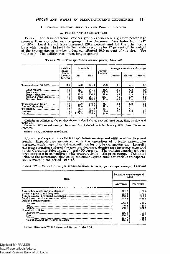
PRICES AND WAGES IN MANUFACTURING INDUSTRIES 1 1 1
II. T r a n s p o r t a t io n S e r v ic e s a n d P u b l ic U t il it ie s
A . PRICES AND EXPENDITURES
Prices in the transportation services group experienced a greater percentage increase than any other service group in the Consumer Price Index from 1947 to 1958. Local transit fares increased 126.4 percent and led the other items by a wide margin. In fact this item which accounts for 27 percent of the weight of the transportation services index, contributed 40.5 percent of the rise. (See table 21.) The utilities rose much less, in general.
T a b l e 21.— Transportation service prices, 1947-58
Relativeimpor
Price index|
PercentAverage annual rate of change
tance, December 1952
1947 1958increase
1947-58 1947-53 1953-58
Transportation services_______ 3.7 89.3 174.1 95.0 6.3 9.1 3.4
Auto repairs______________ 1 .1 95.5 141.9 48.6 3.7 4.3 3.0Insurance_________________ 1 . 0 85.0 171.0 1 0 1 .2 6 . 6 9.8 2 . 8Registration fees__________ .3 97.9 126.9 29.6 2.4 1.3 3.5Bus and transit fares______ 1 .0 8 8 . 8 2 0 1 .0 126.4 7.7 9.9 5.2Railroad fares_____________ .3 89.7 133.2 48.5 3.7 5.4 1.9
Transportation total1_________ 11.3 90.6 140.5 55.1 4.1 6 . 2 1 .6Gas and electricity____________ 1.9 97.6 117.0 19.9 1.7 1 .1 1.9Telephone____________________ 1 .1 95.3 127.4 33.7 2.7 4.4 .7Postage - __ ___________ . 2 97.4 139.9 37.5 2.9 3.6 2 . 1Water _ _ ____________ .3 2 101.3 136.4 34.6 6 .1
1 Includes in addition to the services shown in detail above, new and used autos, tires, gasoline and motor oil.
2 Index for 1953 annual average. Item was first included in index January 1953. Base: December 1952=100.
Source: BLS, Consumer Price Index.
Consumers' expenditures for transportation services and utilities show divergent trends. Expenditures associated with the operation of private automobiles increased much more than did expenditures for public transportation. Intercity rail transportation suffered the greatest decrease, despite fare increases measured by the Consumer Price Index of nearly 50 percent. The utilities experienced very large increases in expenditure with comparatively little price runup. Tabulated below is the percentage changes in consumer expenditures for various transportation services in the period 1947-58.
T a b l e 22.— Expenditures for transportation services, percentage change, 1947-58
Item
Percent change in expenditures
Aggregate Per capita
Automobile repair and maintenance___ . ________________________________ 132.6233.3
76.6175.0Bridge, highway, and ferry tolls____________________________________________
Auto insurance: premiums less claims_______ _________ _____ _______________ 278.2 213.6Local transit, taxi, and communtation____________ ________________________ —5.8 —2 2 . 0Intercity transportation:
Railroad______________________ ________________________________________ —38.7 —49.4Bus.__________________________________________________________________ _ —9.3 —25.1Airline................................................................................................................. 410.0 324.1
Household utilities:Electricity.................................................................. .......... ............................. . 196.5 145.1Gas................................................................................................. ......................... 206.0 153.5Water.................................................................................................... ................... 121.7 83.5Telephone and other communication................................................... ............ 175.2 128.1
Source: Data from “ U.S. Income and Output,” table II-4.
Digitized for FRASER http://fraser.stlouisfed.org/ Federal Reserve Bank of St. Louis
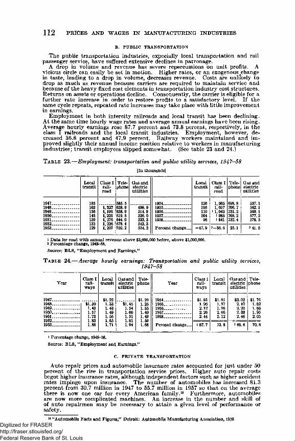
112 PRICES AND WAGES IN MANUFACTURING INDUSTRIES
B. PUBLIC TRANSPORTATION
The public transportation industries, expecially local transportation and rail passenger service, have suffered extensive declines in patronage.
A drop in volume and revenue has severe repercussions on unit profits. A vicious circle can easily be set in motion. Higher rates, or an exogenous change in taste, leading to a drop in volume, decreases revenue. Costs are unlikely to drop as much as revenue because carriers are required to maintain service and because of the heavy fixed cost elements in transportation industry cost structures. Returns on assets or operations decline. Consequently, the carrier is eligible for a further rate increase in order to restore profits to a satisfactory level. If the same cycle repeats, repeated rate increases may take place with little improvement in earnings.
Employment in both intercity railroads and local transit has been declining. At the same time hourly wage rates and average annual earnings have been rising. Average hourly earnings rose 87.7 percent and 73.8 percent, respectively, in the class I railroads and the local transit industries. Employment, however, decreased 36.6 percent and 47.9 percent. Railway workers maintained and improved slightly their annual income position relative to workers in manufacturing industries; transit employees slipped somewhat. (See table 23 and 24.)
T a b l e 23.— Employment: transportation and public utility services, 1947-58
[In thousands]
Localtransit
Class I railroad
Telephone
Gas and electric utilities
Localtransit
Class I railroad
Telephone
Gas and electric utilities
1947........................ 185163166145139133129
585.5638.9638.9619.5 644.0 678.4 702.2
1954........................ 1261161 1 010496
1,065 1,057
i 1,043 *985 1841
698.8706.7751.2768.2 732.4
557.1562.1569.1577.2 578.5
1948.— ................. 1,327 1,191 1 ,2 2 1 1,276 1,226 1,207
498.0 514.9526.0533.3543.3 554.2
1955........................1949........................ 1956 ...............1950........................ 1957........................1951........................ 1958........................1952
Percent change__1953................. ....... -47 .9 2-36.6 25.1 2 41.8
i Data for road with annual revenue above $3,000,000 before, above $1 ,0 0 0 ,0 0 0 .* Percentage change, 1948-68.Source: BLS, “ Employment and Earnings.”
T a b l e 24.— Average hourly earnings: Transportation and public utility services,1947-58
YearClass I
railways
Localtransit
Gas and electric utilities
Telephone Year
Class I railways
Localtransit
Gas and electric utilities
Telephone
1947........................ $1 .2 2 1.33 1.43 1.49 1.56 1.65 1.71
$1 .2 01.251.351.401.491.591 .6 8
1954.................... $1.93 1.96 2 .1 2 2.26 2.44
$1.81 1.87 1.96 2.05 2 .1 2
$2 .0 2 2 .1 0 2 .2 2 2.33 2.46
$1.76 1.82 1 .8 6 1.95 2.05
1948................. ....... $1.301.431.571.731.831 .8 8
$1.45 1.54 1.60 1.51 1.81 1.94
1955 .................1949........................ 1956.....................—1950........................ 1957.....................—1951........................ 1958........................1952
Percent change...1953........................ 187.7 73.8 169.6 70.8
i Percentage change, 1948-68.Source: BLS, “ Employment and Earnings.”
C. PRIVATE TRANSPORTATION
Auto repair prices and automobile insurance rates accounted for just under 50 percent of the rise in transportation service prices. Higher auto repair costs begot higher insurance rates, although independent factors such as higher accident rates impinge upon insurance. The number of automobiles has increased 81.3 percent from 30.7 million in 1947 to 55.7 million in 1957 so that on the average there is now one car for every American family.18 Furthermore, automobiles are now more complicated machines. An increase in the number and skill of of auto repairmen may be necessary to attain a given level of performance or safety.
18 “Automobile Facts and Figures,” Detroit: Automobile Manufacturing Association, 1958Digitized for FRASER http://fraser.stlouisfed.org/ Federal Reserve Bank of St. Louis
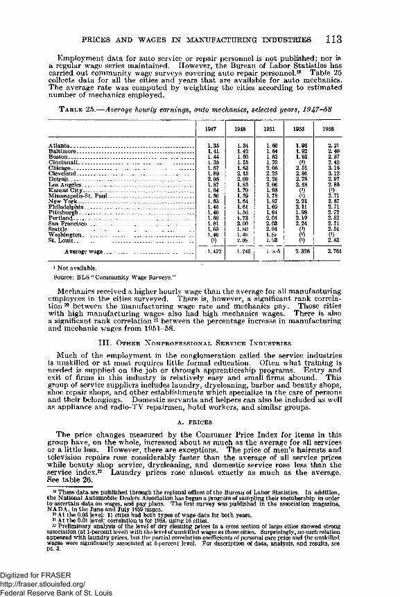
Employment data for auto service or repair personnel is not published; nor is a regular wage series maintained. However, the Bureau of Labor Statistics has carried out community wage surveys covering auto repair personnel.19 Table 25 collects data for all the cities and years that are available for auto mechanics. The average rate was computed by weighting the cities according to estimated number of mechanics employed.
PRICES AND WAGES IN MANUFACTURING INDUSTRIES 113
T a b l e 25.— Average hourly earnings, auto mechanics, selected years, 1947-58
1947 1948 1951 1953 1958
Atlanta_________ __________________ ____ __________ 1.35 1.34 1.60 1.98 2 .2 1Baltimore__________________________________ _____ 1.41 1.42 1.64 1.92 2.40Boston________ _______________ _________________ _ 1.44 1.50 1.63 1.93 2.37Cincinnati__________________________________ ______ 1.35 1.55 1.70 0 )
2. 512.42
Chicago_______________________________ ____________ 1.67 1.83 2.06 3.16Cleveland________________________ _________ ______ 1.89 2.15 2.25 2 . 8 6 3.12Detroit_______________ ________________ _ ___ 2.05 2.09 2.26 2.78 2.97Los Angeles____ . . . _____________________ ____ ____ 1.87 1.85 2.06 2.48 2 .8 6Kansas City......... .................... 1.64 1.70 1.98 0 )
0 )0 )2.71Minneapolis-St. Paul_____________________________ _ 1.50 1.59 1.78
New York_______________________________ _________ 1.53 1.64 1.87 2 .2 1 2.67Philadelphia___________________ ____ _____ _____ 1.45 1.61 1.69 2 .1 1 2.71Pittsburgh____ ________________ . . _______ 1.40 1.56 1.94 1.98 2.72Portland_______ ____ ______________________________ 1.60 1.73 2 .0 1 2.19 2.52San Francisco_____________ . _____________________ 1.81 2 .0 0 2.03 2.24 2.71Seattle. _____ ___________________________________ . . 1.63 1.80 2 .0 1 0 ) 2.54Washington_____________ __________________________ 1.46 1.48 1! 1.81 0 ) 0 )St. Louis_______________________ . ____________ 0 ) 2 .0 8 ! 1.93 |; 0 ) 2.83
Average wage_____________________ _________ 1.479 1.745 1 . 2.328 2.761
1 Not available.Source: BLS “ Community Wage Surveys.”
Mechanics received a higher hourly wage than the average for all manufacturing employees in the cities surveyed. There is, however, a significant rank correlation 20 between the manufacturing wage rate and mechanics pay. Those cities with high manufacturing wages also had high mechanics wrages. There is also a significant rank correlation 21 between the percentage increase in manufacturing and mechanic wages from 1951-58.
I I I . O t h e r N o n p r o f e s s io n a l S e r v ic e I n d u s t r ie s
Much of the employment in the conglomeration called the service industries is unskilled or at most requires little formal education. Often what training is needed is supplied on the job or through apprenticeship programs. Entry and exit of firms in this industry is relatively easy and small firms abound. This group of service suppliers includes laundry, drycleaning, barber and beauty shops, shoe repair shops, and other establishments which specialize in the care of persons and their belongings. Domestic servants and helpers can also be included as well as appliance and radio-TV repairmen, hotel workers, and similar groups.
a . p r ic e s
The price changes measured by the Consumer Price Index for items in this group have, on the whole, increased about as much as the average for all services or a little less. However, there are exceptions. The price of men’s haircuts and television repairs rose considerably faster than the average of all service prices while beauty shop service, drycleaning, and domestic service rose less than the service index.22 Laundry prices rose almost exactly as much as the average. See table 26.
19 These data are published through the regional offices of the Bureau of Labor Statistics. In addition, the National Automobile Dealers Association has begun a program of sampling their membership in order to ascertain data on wages, and pay plans. The first survey was published in the association magazine, NADA, in the June and July 1959 issues.
20 At the 0.03 level: 11 cities had both types of wage data for both years.21 At the 0.01 level: correlation is for 1958, using 16 cities.22 Preliminary analysis of the level of dry cleaning prices in a cross section of large cities showed strong
association (at 1-percent level) with the level of unskilled wages in those cities. Surprisingly, no such relation appeared with laundry prices, but the partial correlation coefficients of personal care price and the unskilled wages were significantly associated at 5-percent level. For description of data, analysis, and results, see pt. 3.
Digitized for FRASER http://fraser.stlouisfed.org/ Federal Reserve Bank of St. Louis
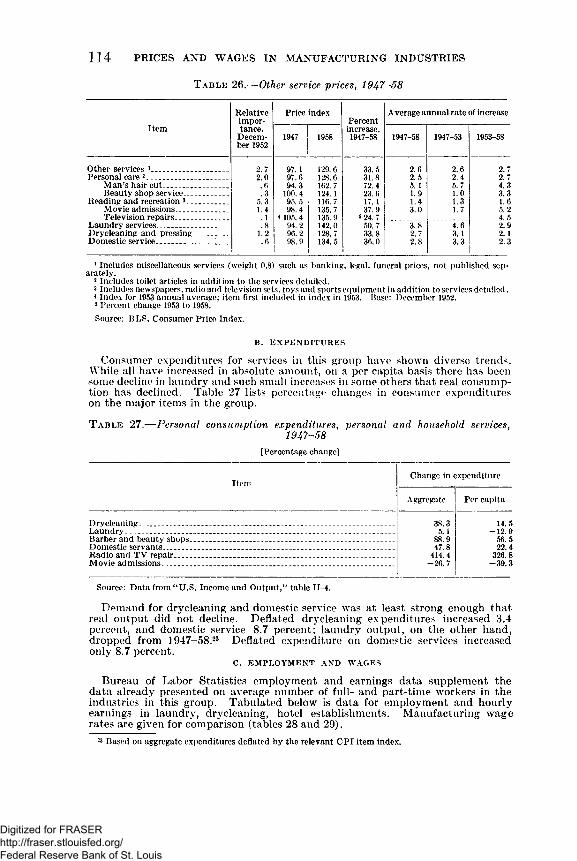
114 PRICES AND WAGES IN MANUFACTURING INDUSTRIES
Table 26.— Other service prices, 1947—58
Item
Relative importance,
December 1952
Price indexPercentincrease,1947-58
Average annual rate of increase
1947 1958 1947-58 1947-53 1953-58
Other services J._____ ____________ 2.7 97.1 129.6 33.5 2 .6 2 . 6 2.7Personal care 2____________________ 2 . 0 97.6 128.6 31.8 2.5 2.4 2.7
Man’s hair cut......................... . . 6 94.3 162.7 72.4 5.1 5.7 4.3Beauty shop service.................. .3 100.4 124.1 23.6 1.9 1 .0 3.3
Reading and recreation 3____ ______ 5.3 95.5 116.7 17.1 1.4 1.3 1 .6M ovie admissions........................ 1.4 98.4 135.7 37.9 3.0 1.7 5.2Television repairs...................... . 1 * 105.4 135.9 5 24.7 4.5
Laundry services......... ................... . 8 94.2 142.0 50.7 3.8 4.6 2.9Drycleaning and pressing_________ 1 .2 96.2 128.7 33.8 2.7 3.1 2 .1Domestic service________ __________ . 6 98.9 134. 5 36.0 2 . 8 3.3 2.3
1 Includes miscellaneous services (weight 0.8) such as banking, legal, funeral prices, not published separately.
2 Includes toilet articles in addition to the services detailed.3 Includes newspapers, radio and television sets, toys and sports equipment in addition to services detailed. < Index for 1953 annual average; item first included in index in 1953. Base: December 1952.5 Percent change 1953 to 1958.Source: BLS, Consumer Price Index.
B. E X P E N D IT U R E S
Consumer expenditures for services in this group have shown diverse trends. While all have increased in absolute amount, on a per capita basis there has been some decline in laundry and such small increases in some others that real consumption has declined. Table 27 lists percentage changes in consumer expenditures on the major items in the group.
T a b l e 27.— Personal consumption expenditures, personal and household services,1947-58
[Percentage change]
ItemChange in expenditure
Aggregate Per capita
Drvcleaning_____________ _________________________ _______ _______________ 38.3 14. 5Laundry____________________________ _____________________ _______ _________ 5.1 -12 .9Barber and beauty shops____ _____________ _______________ _______ ________ 88.9 56.5Domestic servants_________ ________ ___________________________________ . 47.8 22.4Radio and TV repair................................................... .............................................. . 414.4 326.8Movie admissions................. .......................................................... ............ ............ -26. 7 -39 .3
Source: Data from “ U.S. Income and Output,” table II—4.
Demand for drycleaning and domestic service was at least strong enough that real output did not decline. Deflated drycleaning expenditures increased 3.4 percent., and domestic service 8.7 percent; laundry output, on the other hand, dropped from 1947-58.23 Deflated expenditure on domestic services increased only 8.7 percent.
C. EM P LO YM E N T AND W AG ES
Bureau of Labor Statistics employment and earnings data supplement the data already presented on average number of full- and part-time workers in the industries in this group. Tabulated below is data for employment and hourly earnings in laundry, drycleaning, hotel establishments. Manufacturing wage rates are given for comparison (tables 28 and 29).
23 Based on aggregate expenditures deflated by the relevant CPI item index.
Digitized for FRASER http://fraser.stlouisfed.org/ Federal Reserve Bank of St. Louis
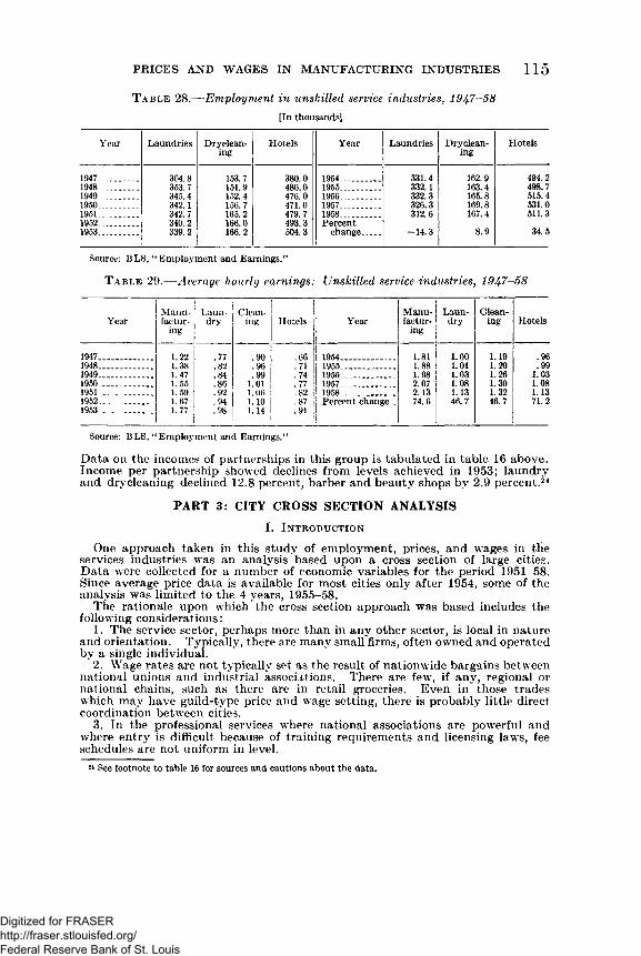
PRICES AND WAGES IN MANUFACTURING INDUSTRIES 115
Table 28.— Employment in unskilled service industries, 1947-58 [In thousands]
Year Laundries Dryclean-ing
Hotels Year Laundries Dryclean-ing
Hotels
1947.............. 364.8 153.7 380.0 1954..,............ 331.4 162.9 494.21948_________ 353.7 151.9 486.0 1955................ 332.1 163.4 498.71949................ 345.4 152.4 476.0 1956.............. 332.3 165.8 515.41950 ____ 342.1 156.7 471.0 1957 .......... 326.3 169.8 531.01951_________ 342.7 165.2 479.7 1958................ 312.6 167.4 511.31952_________ 340.2 166.0 493.3 Percent1953.............. 339.2 j 166. 2 504.3 change....... -14 .3 8.9 34.5
Source: BLS, “ Employment and Earnings.”
Table 29.— Average hourly earnings: Unskilled service industries, 1947-58
YearManufactur
ing
Laun- j Clean- dry i ing Hotels Year
Manufactur
ing
Laundry
Cleaning Hotels
1947.1948.1949.1950. 19511952.1953.
1.221.381.471.551.591.671.77
.77
.82
.84.86
.92
.94
.90
.96
.99 1.01 1.06 1.10 1.14
1954......................1955......................1956......................1957-...................1958....................Percent change..
1.81 1.88 1.98 2.07 2.13 74.6
1.00 1.01 1.03 1.08 1.13 46.7
1.191.20 1.26 1.30 1.32 46.7
1.03 1.08 1.13 71.2
Source: BLS, “ Employment and Earnings.”
Data on the incomes of partnerships in this group is tabulated in table 16 above. Income per partnership showed declines from levels achieved in 1953; laundry and dry cleaning declined 12.8 percent, barber and beauty shops by 2.9 percent.2"4
PART 3: CITY CROSS SECTION ANALYSISI. Introduction
One approach taken in this study of employment, prices, and wages in tlie services industries was an analysis based upon a cross section of large cities. Data were collected for a number of economic variables for the period 1951-58. Since average price data is available for most cities only after 1954, some of the analysis was limited to the 4 years, 1955-58.
The rationale upon which the cross section approach was based includes the following considerations:
1. The service sector, perhaps more than in any other sector, is local in nature and orientation. Typically, there are many small firms, often owned and operated by a single individual.
2. Wage rates are not typically set as the result of nationwide bargains between national unions and industrial associations. There are few, if any, regional or national chains, such as there are in retail groceries. Even in those trades which may have guild-type price and wage setting, there is probably little direct coordination between cities.
3. In the professional services where national associations are powerful and where entry is difficult because of training requirements and licensing laws, fee schedules are not uniform in level.24 See footnote to table 16 for sources and cautions about the data.
Digitized for FRASER http://fraser.stlouisfed.org/ Federal Reserve Bank of St. Louis
II. The D ata
A. CITY SAMPLEThe cities chosen were the 20 large cities for which the Bureau of Labor Sta
tistics (BLS) publishes price data gathered in connection with compilation of the Consumer Price Index. They are listed below:♦Atlanta Minneapolis♦Baltimore *New YorkBoston Pittsburgh
♦Cincinnati ♦Philadelphia♦Chicago Portland, Oreg.Cleveland *St. Louis
♦Detroit ♦San FranciscoHouston ScrantonKansas City Seattle
♦Los Angeles Washington, D.C.♦Price data available for 1952-58.
B. PRICE DATAA yearly average price for each of seven services categories was computed and
used in this study. A simple arithmetic mean was used to summarize all the price quotations within a category into an annual quotation. There are seven prices for each city for each year.
The following are the categories and the items included:Laundry service: Semifinished and finished.Dry cleaning: Man's shirt, delivered and women’s dress, cash and carry. Automobile service: Brake relining and chassis lubrication.Hospital room rates, per day rate for the following types of accommodation: Men’s
pay ward, semiprivate room, private room.Medical service: Office visit to general practitioner, house visit by general prac
titioner, obstetrical case, appendectomy (surgeon’s usual fee excluding anesthetic) .
Dental service: Tooth filling amalgam, one surface; tooth extraction without complication, including X-ray.
Personal-care services: Man’s haircut; shampoo and wrave set, plain, short hair.Monthly prices are given for the five largest cities; the remaining 15 cities are
priced 4 times per year such that five of them are priced each month. All data came from the BLS and can be found in the publications mentioned belowr.
Data for December 1952 and for 1953-54 is from “ Average Retail Prices: Collection and Calculation Techniques and Problems,” Bulletin No. 1182 (June 1955). Only the 10 cities marked with asterisks in the list above are reported. Data for the full 20-city sample for 1955 is given in “ Average Retail Prices/7 Bulletin No. 1197 (June 1956). Data for 1956-58 was taken from BLS worksheets in the Division of Prices and Cost of Living and will be published in the future.
C. UNSKILLED WAGE RATESThere are no wage data available for workers in service industries on a city
basis. The Bureau of Labor Statistics does, however, publish periodically Bulletins in the series entitled “ Occupational Wage Surveys.” Data on wages m office, professional, maintenance, and custodial occupations are given for a number of large cities annually (or at times, less regularly) by these publications.
A composite unskilled wage rate was computed for each city and year using data from the “ Occupational Wage Survey” series. Six occupations were chosen to be representative of the level of skill typically required in unskilled service industries. The average of the wage paid to workers in these six occupations was then used as an estimate of the level of wages paid in unskilled service industries in the same city and year.
The six occupations chosen were male janitors, female janitors, male laborers (material handling), female packers (shipping), office boys, and female file clerks (class B), all employed in nonmanufacturing industries.
116 PRICES AND WAGES IN MANUFACTURING INDUSTRIES
Digitized for FRASER http://fraser.stlouisfed.org/ Federal Reserve Bank of St. Louis
For Washington, D.C., no “ Surveys” have been published by BLS. The salary for the lowest civil service grade, transformed to an hourly rate was used
When data for a year was missing, the gap was filled by interpolating between years. If more than 1 year was missing, the movement of manufacturing wages was used as a guide.
Unskilled wage data was interpolated for the following cities and years:Baltimore: 1953-54, 1956.Boston: 1958.Cleveland: 1953, 1955, 1957.Detroit: 1952, 1954, 1956, 1957.Minneapolis: 1956.Portland: 1954.St. Louis: 1958.Seattle: 1952-55.
No unskilled wage data at all was available for Cincinnati, Pittsburgh, Houston, Kansas City, and Scranton. These cities were removed from all analyses involving wages.
D. MANUFACTURING WAGES AND INDUSTRIAL EMPLOYMENTManufacturing wage rates were supplied by the BLS and are published in its
regular periodical, “ Employment and Earnings.” The May 1954 and May 1959 editions contain annual data which covers the entire period.
Employment is reported for the major nonagricultural divisions: manufacturing, construction, trade, finance, service, government. The manufacturing wage data was not published for the following cities and years: Cincinnati, 1952; Houston, 1952-54; Washington, D.C., 1952-54; Chicago and Cleveland, 1951.
E. LABOR MARKET CONDITION*Major labor markets are classified using a system which takes into account the
level of unemployment, the current labor supply and demand situation, expected short-run requirements for labor, and seasonal factors.
Over the period, the classification scale has been changed; however, since this analysis was based on cross-section data only, the noncomparability of the two scales over time is of no importance.
The labor-market condition is reported bimonthly. The Labor Department’s ranking scheme was translated into numbers and the arithmetic mean of the 6 bimonthly rankings was used to represent the annual labor-market condition for each city and year.
The data may be found in the periodical “ Area Labor Market Trends” (and its predecessor, “ The Bimonthly Summary of Labor Market Developments in Major Areas” ) published by the BLS Bureau of Employment Security.
F. POPULATIONPopulation estimates were taken from the annual May “ Survey of Buying
Power” issue of Sale Management Magazine.
G. PRICE LEVELSince the Consumer Price Index is a measure of the change in prices in relation
to the base period 1947-49, divergences of the index reported for individual cities can show only differential changes in prices. They do not necessarily show differences which may exist in the level of prices among the cities.
To transform the price index from a measure of change only, into a measure of price level, it is necessary to adjust the base-period level to reflect differences in cost among the cities.
In 1946, the BLS conducted a study in which the cost in each city of a standard bill of goods and services (similar in scope to the coverage of the CPI) was determined.
BLS Bulletin No. 927, “ Workers’ Budgets in the United States: City Families and Single Persons, 1946 and 1947,” reports the results of the study. (See table6, pp. 28-30 of the Bulletin.) The mean cost of the budget in the 20-city sample was computed. The cost of the budget in each of the cities was then converted
PRICES AND WAGES IN MANUFACTURING INDUSTRIES 117
Digitized for FRASER http://fraser.stlouisfed.org/ Federal Reserve Bank of St. Louis
118 PRICES AND WAGES IN MANUFACTURING INDUSTRIES
into an index with base equal to the average cost of the budget in the 20 cities. The results are tabulated below.
Table 30.- - Cost of a standard budget for a fam ily of 4, selected sample of cities, 1946
[Index numbers]Atlanta________________________ _101. 0Baltimore_______________________105. 0Boston__________________________106. 7Chicago_________________________104. 8Cincinnati_____________________ _100. 5Cleveland_______________________101. 8Detroit________________________ _105. 6Houston_______________________ 95. 0Kansas City___________________ 97. 7Los Angeles_____________________103. 8
Note.—Base is average of cost of budget in all cities.
Minneapolis___________________ 104. 3New York_____________________ 105. 8Philadelphia___________________ 100. 6Pittsburgh_____________________ 103. 6Portland_______________________ 103.3St. Louis_______________________ 106. 0San Francisco__________________ 107. 1Scranton_______________________ 98. 5Seattle_________________________ 109. 3Washington, D.C______________ 112. 0
To this base was added the Consumer Price Index as reported by the BLS for each city and year. The new index shows price change adjusted for differences in price level in the individual cities.
H. NON WHITE POPULATIONPercentage of population which is non white was taken directly from the ‘ ‘Coun
try and City Data Book, 1956” (Bureau of the Census), table 3. The data refer to the year 1950 and were collected in connection with the regular decennial census.
III. Preliminary Analysis
The data described above were used in an attempt to gain understanding of the variables and mechanisms important in price and wage making in the services industries. The results are probably more suggestive than definitive for various reasons mentioned below.
All data in a cross-section should represent simultaneous observations of all variables in all elements of the sample. In the data used here, the observations are considered to be annual averages. But some of the variables are averages of 12 observations; some of 6; some of 4 observations, not all of which refer to the same date in all cities; some, in the case of unskilled wages, are only one observation per year. In years of rapidly changing conditions, the month in which the “ representative” observation falls might make important difference in results, especially when all the cities are not surveyed the same month.24a
Errors of observation are probably quite high in much of the data used. While the BLS does publish average price data drawn from their price observations for the Consumer Price Index, it must be remembered that main concern of the BLS is with measuring changes in price. If it becomes necessary to alter the sample of establishments surveyed, it makes little difference in the index-making process if, other things equal, the average price differs between the two establishments. As long as successive monthly changes have been the same, the new outlet can be linked smoothly into the index. The average price data may however show an abrupt change.
Combining the labor-market index into an annual average suppresses much of its sensitivity. If it were feasible to collect the rest of the data on a quarterly basis, use of a quarterly labor market condition indicator would be better. Other difficulties include the small number of service occupations for which data were available, as well as the limited number of cities and years included.
Nevertheless preliminary results of what has been found to date are summarized briefly here. Negative results as well as more encourging ones are indicated.
24a It is conceivable that something like the following could be true: assume that two cities in fact have the same average wage rate and that in both cities the wage-rate increases in uniform, 2-cent-per-month increments. Xow, if the first city were surveyed in January and the second city in December, the second city would show a wage 24 cents higher than the first. Taking simple first difference would not solve the problem because the given city is not always surveyed in the same month each year by BLS. Sometimes the “annual” first difference might span an interval of less than a year, sometimes more.
Digitized for FRASER http://fraser.stlouisfed.org/ Federal Reserve Bank of St. Louis
PRICES AND WAGES IN MANUFACTURING INDUSTRIES 119
A. WAGESThe first general hypothesis for investigation was that the industrial composition
of the labor force, the labor-market condition, and the price level explain the level of manufacturing or unskilled wages.
Three regressions were run. Two attempted to explain the level of unskilled wages; one of manufacturing wages. The first regressed the level of unskilled wages on the percentage of the total labor force accounted for by employment in the service sector,25 the labor-market condition (LMC), and the price level.
The second regressed the unskilled wage level on the percentage of total employed in the services industries, the LMC, and the price level. The third regression investigated the association of manufacturing wages on percentage of the total labor force employed in industrial employment, the condition of the labor market and the price level.
The coefficients of multiple determination (R2) associated with the manufacturing wage regression were significant at the 5-percent level for the years 1956-58, and nearly so in 1955. The beta coefficients associated with the price level were significant at the 5-percent level in 1955 and at the 1 percent level in 1957-58. In addition, in 1957 and 1958 the beta for labor-market condition was significant at the 5-percent level. (See appendix tables.)
On the other hand, the regression of unskilled wages on the variables named above had no coefficients of multiple determination which were significant. The betas associated with labor-market condition and price level were significant at the 5-percent level in 1958 in the regression which included service sector employment as one of the independent variables. The regression involving services industries employment as a variable had no significant betas. (See appendix tables 1 and 2.)
B. SPILLOVER INVESTIGATIONIf the level of unskilled wages cannot be satisfactorily explained by employ
ment structure, labor market condition, or price level, another hypothesis is available. That is the “ spillover’ ’ thesis.
The form investigated here states that the level and change in unskilled wages are associated with the level and change in manufacturing wages more than with other explanatory variables.
The analysis was carried out using rank correlation methods developed by Kendall.26 The coefficient of rank correlation is called tau by Kendall and will be used throughout as a shorthand expression.
A sample of 14 cities was used, including Atlanta, Baltimore, Boston, Chicago, Cleveland, Detroit, Los Angeles, Minneapolis-St. Paul, New York, Philadelphia, Portland, St. Louis, San Francisco, and Seattle.27Level of unskilled wage on level of manufacturing wage
The results of correlation of cities ranked by level of unskilled wages and level of manufacturing wages were extremely significant. The correlations were carried out using data for the years 1951-58. The size of the sample is 14 cities for each set of computations reported. Cities omitted were Cincinnati, Houston, Kansas City, Pittsburgh, Scranton, and Washington, D.C.
The values of tau and the significance level associated with each one are tabulated below:
Rank correlation coefficients
YearValue of
coefficientLevel at which
significantYear
Value of coefficient
Level at which
significant
1951_________________ 0.7023 .7079 .6630 .6742
0.0006.0003.0006.0006
1955............- .................. 0.5889.7300.7889.6409
0.0024.0 0 0 1.0 0 0 1.0009
1952_______ __________ 1956 ____ ____1953_________________ 1957............- ..................1954______ __________ 1958...............................
25 That is, the services industries, finance and insurance, transportation and public utilities.26 M. G. Kendall, “ Rank Correlation Methods,” London: Charles Griffin & Co., 1948. The method set
forth by Kendall has the advantage over the simpler Spearman method for small samples. The distribution of tau tends to normality for samples greater than 10 and has been computed for values under 1 0 .
27 It will be noted that some of these cities have interpolated unskilled wage rates for some years. The first correlation reported below used both interpolated and uninterpolated data. No significant differences arose, so interpolated data was used throughout.
Digitized for FRASER http://fraser.stlouisfed.org/ Federal Reserve Bank of St. Louis
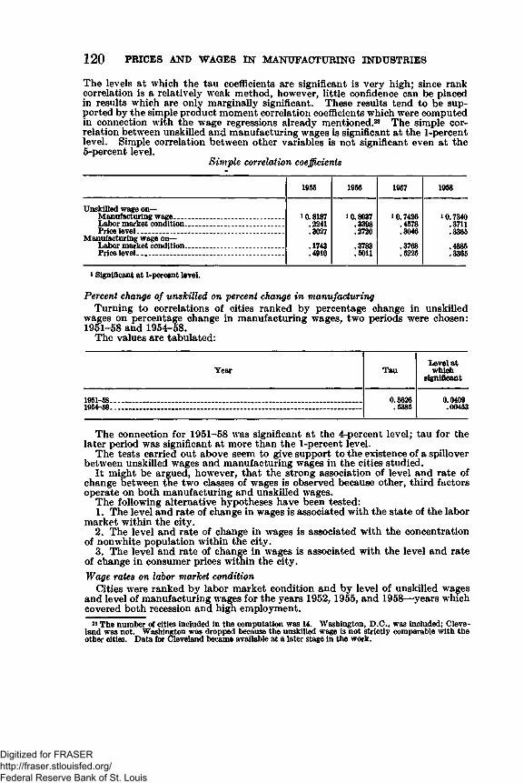
The levels at which the tau coefficients are significant is very high; since rank correlation is a relatively weak method, however, little confidence can be placed in results which are only marginally significant. These results tend to be supported by the simple product moment correlation coefficients which were computed in connection with the wage regressions already mentioned.28 The simple correlation between unskilled and manufacturing wages is significant at the 1-percent level. Simple correlation between other variables is not significant even at the 5-percent level.
Sim ple correlation coefficients
120 PBICES AND WAGES IN MANUFACTURING INDUSTRIES
1965 1956 1957 1958
Unskilled wage on—Manufacturing wage.......................................................Labor market condition.................................................Price level ________ . . . __
1 0.8187 .2241 .3027
.1743
.4910
t0 .8037 .3398 .2720
.3783
.5011
10.7426 .4578 .3046
.3768
.5225
10.7340.3711.3365
.4885
.3365
Manufacturing wage on—Labor market condition.................................................Price level..... ....................................................................
1 Significant at 1-percent level.
Percent change of unskilled on percent change in m anufacturing
Turning to correlations of cities ranked by percentage change in unskilled wages on percentage change in manufacturing wages, two periods were chosen: 1951-58 and 1954-58.
The values are tabulated:
Year TauLevel at which
significant
1951-58.............................................................................................................................. 0.3626 0.04091954-58.............................................................................................................................. .5385 .00453
The connection for 1951-58 was significant at the 4-percent level; tau for the later period was significant at more than the 1-percent level.
The tests carried out above seem to give support to the existence of a spillover between unskilled wages and manufacturing wages in the cities studied.
It might be argued, howrever, that the strong association of level and rate of change between the two classes of wages is observed because other, third factors operate on both manufacturing and unskilled wages.
The following alternative hypotheses have been tested:1. The level and rate of change in wages is associated with the state of the labor
market within the city.2. The level and rate of change in wages is associated with the concentration
of nonwhite population within the city.3. The level and rate of change in wages is associated with the level and rate
of change in consumer prices within the city.Wage rates on labor market condition
Cities were ranked by labor market condition and by level of unskilled wages and level of manufacturing wages for the years 1952,1955, and 1958— years which covered both recession and high employment.
« The number of cities included in the computation was 14. Washington, D .C., was included; Cleveland was not. Washington was dropped because the unskilled wage is not strictly comparable with the other cities. Data for Cleveland became available at a later stage in the work.
Digitized for FRASER http://fraser.stlouisfed.org/ Federal Reserve Bank of St. Louis
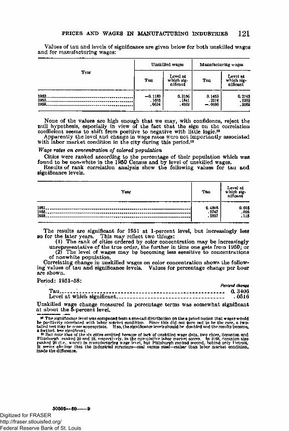
PRICES AND WAGES IN MANUFACTURING INDUSTRIES 121
Values of tau and levels of significance are given below for both unskilled wages and for manufacturing wages:
Year
Unskilled wages Manufacturing wages
TauLevel at
which significant
TauLevel at
which significant
1952............................................................................... -0.1189 .1695 .0634
0.3156.1841.4562
0.1453 .2374
-.0586
0.2743.1292.3669
1955...............................................................................1958...............................................................................
None of the values are high enough that we may, with confidence, reject the null hypothesis, especially in view of the fact that the sign on the correlation coefficient seems to shift from positive to negative with little logic.29
Apparently the level and change in wage rates were not importantly associated with labor market condition in the city during this period.30Wage rates on concentration of colored population
Cities were ranked according to the percentage of their population which was found to be non-white in the 1950 Census and by level of unskilled wages.
Results of rank correlation analysis show the following values for tau and significance levels.
Year TauLevel at
which significant
1951............................................................................................... ................................... 0.4505 0.0151955________________________________________________________________________ .2747 .0951958................................................................................................................................... .2527 .115
The results are significant for 1951 at 1-percent level, but increasingly less so for the later years. This may reflect two things:
(1) The rank of cities ordered by color concentration may be increasingly unrepresentative of the true order, the further in time one gets from 1950; or
(2) The level of wages may be becoming less sensitive to concentrations of nonwhite population.
Correlating change in unskilled wages on color concentration shows the following values of tau and significance levels. Values for percentage change per hour are shown.Period: 1951-58:
Percent changeTau.......... 1................................................................................................... 0.3406Level at which significant________________________________________ .0516
Unskilled wage change measured in percentage terms was somewhat significant at about the 5-percent level.
*• The significance level was computed from a one-tail distribution on the a priori notion that wages would be positively correlated with labor market condition. Since this did not turn out to be the case, a two* tailed rest may bi* rrore appropriate. If so, the significance levels should be doubled and the results become, a fortiori, less significant.
80 But note that of the six cities omitted because of lack of unskilled wage data, two cities, Scranton and Pittsburgh ranked 20 and 18, respectively, in the cumulative labor market scores. In 1958, Scranton also ranked 20 (i.e.. worst) in manufacturing wage level, but Pittsburgh ranked second, behind only Detroit. It seems obvious that the industrial structure—coal versus steel—rather than labor market condition, made the difference.
50505— 60------ 9Digitized for FRASER http://fraser.stlouisfed.org/ Federal Reserve Bank of St. Louis
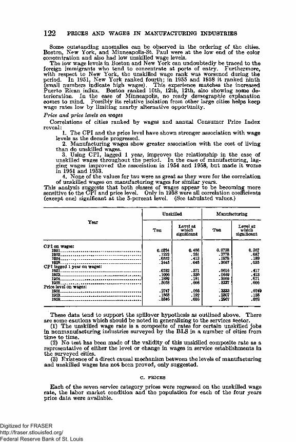
Some outstanding anomalies can be observed in the ordering of the cities. Boston, New York, and Minneapolis-St. Paul were at the low end of the color concentration and also had low unskilled wage levels.
The low wage levels in Boston and New York can undoubtedly be traced to the foreign immigrants who tend to concentrate at ports of entry. Furthermore, with respect to New York, the unskilled wage rank was worsened during the period. In 1951, New York ranked fourth; in 1955 and 1958 it ranked ninth (small numbers indicate high wages). This experience matches the increased Puerto Rican influx. Boston ranked 10th, 12th, 12th, also showing some deterioration. In the case of Minneapolis, no ready demographic explanation comes to mind. Possibly its relative isolation from other large cities helps keep wage rates low by limiting nearby alternative opportunity.Price and price levels on wages
Correlations of cities ranked by wages and annual Consumer Price Index reveal:
1. The CPI and the price level have shown stronger association with wage levels as the decade progressed.
2. Manufacturing wages show greater association with the cost of living than do unskilled wages.
3. Using CPI, lagged 1 year, improves the relationship in the case of unskilled wages throughout the period. In the case of manufacturing, lagging wages improved the association in 1954 and 1958, but made it worse in 1951 and 1953.
4. None of the values for tau were as great as they were for the correlation of unskilled wages on manufacturing wages for similar years.
This analysis suggests that both classes of wages appear to be becoming more sensitive to the CPI and price level. Only in 1958 were all correlation coefficients (except one) significant at the 5-percent level. (See tabulated values.)
122 PRICES AND WAGES IN MANUFACTURING INDUSTRIES
Unskilled Manufacturing
Year
TauLevel at which
significantTau
Level at which
significant
CPI on wages:1951....................................................................... 0.0324 0.456 0.0738 0.3671953....................................................................... .1222 .251 .2778 .0871954.......................~ .................................. .......... .0552 .413 .1878 .1891958....................................................................... .3445 .045 .3667 .035
CPI lagged 1 year on wages:1951....................................................................... .0782 .371 .0615 .4171953..................................................... ................. .1006 .330 .0559 .4131954....................................................................... .1889 .181 .3000 .0711958....................................................................... .5058 .008 .5337 .006
Price level on wages:1951....................................................................... .2747 .095 .3333 . 07491953....................................................................... .1868 .192 .2307 .1381958........................................................................ .3846 .036 .2967 .078
These data tend to support the spillover hypothesis as outlined above. There are some cautions which should be noted in generalizing to the services sector.
(1) The unskilled wage rate is a composite of rates for certain unskilled jobs in nonmanufacturing industries surveyed by the BLS in a number of cities from time to time.
(2) No test has been made of the validity of this unskilled composite rate as a representative of either the level or change in wages in service establishments in the surveyed cities.
(3) Existence of a direct causal mechanism between the levels of manufacturing and unskilled wages has not been proved, only suggested.
c. PRICES
Each of the seven service category prices were regressed on the unskilled wage rate, the labor market condition and the population for each of the four years price data were available.
Digitized for FRASER http://fraser.stlouisfed.org/ Federal Reserve Bank of St. Louis
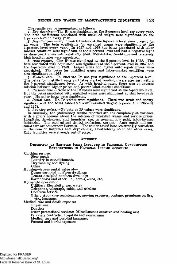
The results can be summarized as follows:1. Dry cleaning.— The R2 was significant at the 5-percent level for every year.
The beta coefficients associated with unskilled wages were significant at the 1 percent level in every year.
2. Hospital care.—Significant R2 values at the 5-percent level were present for all years. The beta coefficients for unskilled wages were significant at the 1-percent level every year. In 1957 and 1958 the betas associated with labor market condition were significant at the 5-percent level and had a negative sign: in these years cities with relatively good labor-market conditions and relatively high hospital rates were associated.
S. Auto repairs.— The R2 was significant at the 5-percent level in 1958. The beta associated with population was significant at the 5-percent level in 1957 and the 1-percent level in 1958. Larger cities and higher auto repair prices were associated. The betas for unskilled wages and labor-market condition were also significant in 1958.
4. Medical care.— In 1958 the R2 was just significant at the 5-percent level. The betas for unskilled wage and labor market condition were also just within the 5-percent significance level. As with hospital rates, there was an inverse relation between higher prices and poorer labor-market conditions.
5. Personal care.—None of the R2 values were significant at the 5-percent level. But the betas associated with unskilled wages were significant at that level each year. No other betas were significant.
6. Dental care.—No R2 values were significant. There was weak and spotty significance of the betas associated with unskilled wages: 5 percent in 1955-56 and 1958.
7. Laundry prices.— No beta or R2 values were significant.In summary, the preliminary results reported are not completely at variance
with a priori notions about the relation of unskilled wages and service prices. Hospitals, drycleaners, and laundries are, in general, low paid, labor-intense industries. The medical and dental professions are not. Auto repair and personal care are somewhere between. The results found here are strongly consistent in the case of hospitals and drycleaning; satisfactorily so in the other cases. Only laundries were strongly out of place.
A p p e n d i x
D e f i n it io n o f S e r v ic e s I t e m s I n c l u d e d i n P e r s o n a l C o n s u m p t io n E x p e n d i t u r e s i n N a t i o n a l I n c o m e A c c o u n t s
Clothing service:Shoe repairLaundry in establishments Drycleaning and dyeing Other
Housing—Space rental value of—Owner-occupied nonfarm dwellings Tenant-occupied nonfarm dwellings Farmhouses and other, i.e., hotels, clubs, etc*
Household operation:Utilities: Electricity, gas, water Telephone, telegraph, cable, and wireless Domestic serviceOther: Appliance maintenance, moving expenses, postage, premiums on fire,
etc., insurance Medical care and death expense:
PhysiciansDentistsOther professional services: Miscellaneous curative and healing arts Privately controlled hospitals and sanitariums Medical care and hospital insurance Funeral and burial expenses
PRICES AND WAGES IN MANUFACTURING INDUSTRIES 123
Digitized for FRASER http://fraser.stlouisfed.org/ Federal Reserve Bank of St. Louis
Personal business:Brokerage charges and interest, investment counseling Bank service charges, trust services, safe deposit box rent Services rendered without payment by financial intermediaries, except life
insurance companies Expense of handling life insurance Legal services Interest on personal debtOther: Money orders, net union dues, classified ads., etc.
Transportation:User-owned transportation:
Automobile repair, greasing, washing, parking, etc.Bridge, tunnel, ferry, and road toll Automobile insurance premiums less claims paid
Purchased local transportation:Street and electric railway and local bus TaxicabsRailway commutation
Purchased intercity transportation:Railway Intercity bus Airline Other
Recreation:Radio and TV repair Motion-picture admissions Legitimate theater and opera, etc.Spectator sportsClubs and fraternal organizationsCommercial participant amusements: Billiard parlors, bowling alleys, etc.Parimutuel net receiptsOther
Private education and researchReligious and welfare activitiesForeign travel and remittances
Source: “ U.S. Income and Output,” pp. 150-1, table II-4.
D e f i n it io n o f S e r v ic e I n d u s t r y a s U s e d i n G r o s s P r o d u c t O r i g in a t in g D a t a
Source: Standard Industrial Classification Manual.
Hotels and other lodging places: Includes commercial establishments and institutions engaged in furnishing lodging, or lodging and meals, and camping facilities and space, on a fee basis.
Personal services: Includes establishments primarily engaged in providing services generally involving the care of the person or his apparel, such as laundries, cleaning and dyeing plants, photographic studios, barber and beauty shops, and cleaning and pressing shops.
Private households: Includes private households which employ workers who serve on or about the premises in occupations usually considered as domestic service. Households classifed in this major group iray employ individuals, such as cooks, maids, butlers, personal secretaries, and rranarers of personal affairs; and outside worlers such as gardeners, caretalers, and other maintenance worl ers. Laundresses performing work in their own homes or in the homes of others are included.
Commercial and trade schools and employment agencies: Pusiness and commercial education schools, civil service schools; placement arencies; trade schools.
Business services: Includes establishments rendering services not elsewhere classifed to business enterprises on a fee or contract basis. (Advertising, consumer credit reporting, duplicating, mailing and stenographic services, services to buildings, news syndicates, etc.).
Miscellaneous repair services and hand trades: Includes establishments engaged in miscellaneous repair services. It does not include auto repair, custom work, and shoe repair.
Motion pictures: Includes establishments producing and distributing motion- picture films, exhibiting motion pictures in commercially operated theaters, and furnishing services to the motion picture industry.
Amusement and recreation, except motion pictures: Includes establishments whose primary function is to provide amusement or entertainment on payment
124 PRICES AND WAGES IN MANUFACTURING INDUSTRIES
Digitized for FRASER http://fraser.stlouisfed.org/ Federal Reserve Bank of St. Louis
of a fee or admission eharge, except motion pictures. (Including museums, zoological gardens.)
Medical and other health services: Includes establishments primarily engaged in furnishing medical, surgical, and other health services to persons. Associations or groups primarily engaged in providing medical or other health services to members are included, but not those which limit their services to the provision of insurance against hospitalization or medical costs.
Legal services: Establishments engaged in offering legal advice or legal services on a contract or fee basis, the head or heads of which are members of the bar.
Engineering and other professional services: Establishments performing services by engineers, architects, accountants, artists, lecturers, and writers; also includes nonprofit educational and scientific research agencies.
Educational services: Establishments furnishing formal academic or technical courses, and libraries.
Nonprofit membership organizations: Organizations operating on a nonprofit membership basis for the promotion of the interests of the members.
Table 1.— Regression coefficients, manufacturing wage regression
PRICES AND WAGES IN MANUFACTURING INDUSTRIES 125
Manufacturing wage on—1955 industrial employment.
Labor-market condition. Price level........................ .
1956 industrial employment. Labor-market condition. Price level_____________
1957 industrial employment. Labor-market condition. Price level_____________
1958 industrial employment. Labor-market condition. Price level_____________
Regressioncoefficient
Partial correlation co
efficient
Beta coefficient
Standard error of
beta
Value of R2
0.0065 0.4019 0.3952 0.2598 0.4389.1081 .3134 .3094 .2705.0285 ♦.5748 ♦.5776 .2373.0236 ♦♦. 9160 ♦*. 9122 .1152 ♦.8478.0373 .0751 .0769 .2946.0029 .1242 .1272 .2935.0076 .5217 .4070 .1921 ♦.6093.1705 ♦.5670 ♦.4895 .2052.0319 ♦♦.6676 ♦♦.6060 .1950.0014 .0923 .0693 .2159 ♦.6531.1925 ♦♦.6785 ♦♦.7393 .2310.0335 ♦♦.7004 ♦♦.6293 .1851
* Significant at 5-percent level.•♦Significant at 1-percent level.Note.—For R2 to be significant at 5 percent it must equal 0.4660*
Table 2.— Regression coefficients, unskilled wage regressions
Regressioncoefficient
Partial correlation co
efficient
Beta coefficient
Standard error of
beta
Value of R*
1. Unskilled wages on—1955 service-sector employment_______ 0.0061 0.1731 0.1715 0.3085 0.2469
Labor-market condition.......... ......... .1660 .4133 .4661 .3246Price level________________________ .0281 .4549 .5138 .3180
.29831956 service-sector employment_______ . 0 0 1 2 .0345 .0326 .2128Labor-market condition...... ............ .1153 .3803 .3827 .2942Price level........................................... .0171 .3291 .3198 .2901
.26241957 service-sector employment............. .0 0 1 0 .0304 .0253 .403$Labor-market condition................... .1874 .5741 .5841 .2634Price level............................................ .0256 .4818 .4638 .2667
.31191958 service-sector employment............. .0150 .3287 .3433 .4392Labor-market condition__________ .1783 ♦.5989 ♦. 7554 .3193Price level............................................ .0360 ♦. 5912 ♦. 6678 .2880
.2882% Unskilled wages on—
1955 personal-services employment Labor-market condition...................
.0097 .1088 .0997 .2328.1489 .3942 .4181 .3081Price level........................................... .0258 .4384 .4714 .30551956 personal-services employment
Labor-market condition........ ..........—.0042 -.0463 -.0424 .2891 .2136.1095 .3680 .3634 .2904
Price level......................... ................ .0165 .3262 .3089 .2830.2503
— -1957 personal-services employment -.0096 - . 1174 -.0936 .4112Labor-market condition...... ............ .1788 .5654 .5571 .2569
Price level...................................... ..... .0242 .4756 .4376 .2559.28921958 personal-services employment____ .0 1 1 0 .1089 . 1 0 0 2 .3787Labor-market condition...... ............ .1393 .5223 .5902 .3046
Price level............................................ .0289 .5286 .5370 .2739
♦Significant at 5-percent level.Note.—None significant. To be significant at 5 percent, R2 must equal 0.5267.
50505— 60--------10Digitized for FRASER http://fraser.stlouisfed.org/ Federal Reserve Bank of St. Louis
126 PRICES AND WAGES IN MANUFACTURING INDUSTRIES
T a b le 3.— Regression coefficients: Price regression
Regressioncoefficient
Partial correlation co
efficient
Beta coefficient
Standard error of
beta
Value of R2
Laundry prices on—195 unskilled wages ________ ____ 3.2032 0.4901 0.4951 0.2784 0.3097
Labor-market condition__________ - . 2741 —.1370 -.1190 .2719Population_______________________ .0007 .2057 .1835 .2761
1956 unskilled wages__________________ 3.2201 .4780 . 4838 .2811 .3451Labor-market condition__________ .2185 .1254 .1090 .2725Population____ __________________ .0005 .1648 .1412 . 2673
1957 unskilled wages.................. ........... 2.6368 .4471 .4426 .2799 .4061Labor-market cndition___„_______ .4838 .2775 . 2531 . 2770.Population_______________________ .0003 .1 1 0 1 .0903 .25177
1958 unskilled wagese_ _ _ .................. 3.1123 .4786 .4828 .2800 .3818Labor-market condition__________ .1189 .0919 .0781 .2677Population_______________________ .0009 .2529 .2161 .2614
Cleaning prices on—1965 unskilled wages ____ , _______ ___ 1.3849 * 9232 *. 9634 .1267 **. 8969
Labor-market condition__________ .0031 .0153 .0060 .1237Population_______________________ — .0 0 0 2 -.0583 - . 2833 .1257
1956 unskilled wages . „ ____________ 1.3822 *.8785 *. 9259 . 1591 **.7900Labor-market condition__________ -.0016 -.0072 -.0035 .1543Population_______________________ -.0003 5616 3249 .1513
1957 unskilled wages ....... ................ 1.3111 *.8789 * 9708 .1665 **.7898Labor-market condition................... 0504 - . 2178 - . 1163 .1648Population_______________________ —.0003 - . 5284 - . 3018 .1533
1958 unskilled wages__________________ 1.3030 * 9089 *. 9951 .1443 **. 8358Labor-market condition__________ 0339 2438 - . 1097 .1380Population______________________ _ - . 0 0 0 2 - . 5043 -.2488 .1347
Auto-repair prices on—1955 unskilled wages__________________ .1358 .2304 .2096 .2799 .3024
Labor-market condition________ _ .0458 .2241 .1987 .2733Population______________________ _ .0 0 0 1 .3811 .3619 .2776
1956 unskilled wages__________________ .4742 .1918 .2025 .3276 .1106Labor-market condition_______ __ -.0203 -.0287 -.0288 .3175Population____ __________________ .0003 .2195 .2217 .3115
1957 unskilled wages__________________ .1650 .2248 .1939 .2657 .4651Labor-market condition_______ __ -.0151 -.0665 -.0554 .2629Population__________ ____________ .0003 ** 6240 **6177 .2445
1958 unskilled wages_______________ __ .4832 *. 7806 *. 5315 .1345 **.8572Labor-market condition__________ 1018 *-.7593 * - . 4748 .1286Population____________ __________ .0004 * 8442 *.6256 .1256
Personal-care prices on—1955 unskilled wages____________ . ____ .7564 **. 6819 **. 7076 .2399 .4873
Labor-market condition______ . __ —. 1027 -.3421 - . 2698 .2343Population_______________________ — .0 0 0 2 -.3664 -.2964 .2379
1956 unskilled wages__________________ .8863 **. 6726 **. 7147 .2786 .4878Labor-market condition__________ —.0532 - . 1877 - . 1457 .2410Population________________ ______ —.0003 —. 4946 —. 4255 .2364
1957 unskilled wages_______________ . . . .8468 **.6398 **. 7251 . 2754 .4252Labor-market condition__________ —.1066 - . 3133 -.2844 .2726Population_______________________ — .0 0 0 2 - . 3534 -.3029 . 2535
1958 unskilled wages__________________ . 7650 **. 6202 **. 6938 .2774 .3931Labor-market condition__________ —.0443 -.1988 —.1702 .2653Population_____ _________________ — .0 0 0 2 -.3368 - . 2930 .2590
Dental-care prices on—1 9 5 5 unskilled wages__________________ 4.4376 **. 6343 **. 6689 .2578 .4085
Labor-market condition__________ —. 1008 - . 0535 -.0426 . 2517Population_______________________ —.0004 -.1398 - . 1141 . 2556
1956 unskilled wages__________________ 5.0280 **. 6140 **. 6721 .2732 .3815Labor-market condition__________ -.3447 - . 1797 - . 1530 .2648Population_______________________ —.0004 —. 1217 - . 1007 . 2598
1957 unskilled wages__________________ 4.2909 .5451 .6130 .2981 .3268Labor-market condition__________ —. 0986 - . 0469 - . 0438 .2950Population_______________________ —. 0005 -.1395 - . 1223 .2743
1958 unskilled wages__________________ 5.3972 **.6810 **. 7496 . 2548 .4881Labor-market condition__________ —.7583 —.5012 -.4463 .2436Population_____________________ _ -.0004 1138 -.0861 .2378
Hospital-care prices on—1955 unskilled wages_____________ - ____ 1.6388 * 7566 *7615 .2081 **.6144
Labor-market condition__________ —.1419 —. 2768 —. 1851 .2031Population_______________________ .0 0 0 2 .1948 .1296 .2063
1956 unskilled wages__________ _______ 1.8774 *.8035 *. 8495 .1990 **. 6717Labor-market con d ition ........__ —. 2145 —.4670 —.3222 .1929Population_________ ___. . . . . . . . . . . .0 0 0 1 .1170 . 0705 .1892
1957 unskilled wages__________ _____ __ 1.7273 *. 7864 *. 8602 .2136 **. 6542Labor-market condition..________ —. 3379 6172 **—. 5245 .2114Population_________ ________ ____ .0 0 0 2 .2196 .1399 .1966
1958 unskilled wages_______ __________ 1.6474 *. 7446 *.7909 .2242 **.6038Labor-market condition.._______ —. 2356 * * - . 5773 **—.4794 .2143Population........................................... .0 0 0 1 .0983 .0653 .2092
See footnotes at end of table, p. 127.
Digitized for FRASER http://fraser.stlouisfed.org/ Federal Reserve Bank of St. Louis
PRICES AND WAGES IN MANUFACTURING INDUSTRIES 127T able 3.— Regression coefficients: Price regression— Continued
Regressioncoefficient
Partial correlation co
efficient
Beta coefficient
Standard error of
betaValue of
Medical-care prices on—1955 unskilled wages_________________
Labor-market condition..................Population_____________________
0.2360 -.0690
.0000
. 2637 -.0826
.0001
.2709 -.1009
.0001
.3363 -.0914
.0001
0.4183 -.3610
.1624
.4367 -.4618
.2079
.4994 -.5601
.4113 ♦♦.5987
♦♦-.6692 .2319
0.4181-.3431
.1482
.4396-.4572
.1830
.4955-.5751
.3570**.5693
**—.6558.1695
0.2870.2803.2847.2864.2776.2723.2718.2689.2501.2408.2302.2248
0.2663
1956 unskilled wages_________________Labor-market condition..................Population_____________________
.3202
1957 unskilled wages________________Labor-market condition____ _____Population_________ ___________
.4403
1958 unskilled wages________________Labor-market condition__________Population_____________________
**.5428
♦Coefficient is significant at 1-percent level.**Coefficient is significant at 5-percent level.Note.—To be significant at 5 percent R2 must equal .5267.
Digitized for FRASER http://fraser.stlouisfed.org/ Federal Reserve Bank of St. Louis

Digitized for FRASER http://fraser.stlouisfed.org/ Federal Reserve Bank of St. Louis
TECHNICAL NOTE NO. 2 PRODUCTIVITY AND OUTPUT IN THE
POSTWAR PERIOD (BY THOMAS A. WILSON)
129
Digitized for FRASER http://fraser.stlouisfed.org/ Federal Reserve Bank of St. Louis

Digitized for FRASER http://fraser.stlouisfed.org/ Federal Reserve Bank of St. Louis
By Thomas A. Wilson
I. I ntroductionChapter 3 of the “ Staff Report on Employment, Growth, and Price Levels”
includes a discussion of the relationship between productivity and output in the economy.1 Much of that analysis focuses on the effects of intersectoral labor movements upon the rate of growth of aggregate productivity. The underlying data for that portion of the analysis are presented in the report.
Conclusions drawn about the relationship between output and productivity within the major sectors of the economy, however, were partly based upon new data gathered and analyzed by the committee staff. This paper’s purpose is to present and discuss the productivity and output data obtained by the committee staff, together with an analysis of the relationship between output and productivity within the manufacturing sector of the economy.
II. The E stimatesA. MAJOR SECTOR ESTIMATES
Table 1 presents output, man-hour input, and productivity indexes for the major sectors of the economy. The reader must be forewarned, however, that productivity estimates are only as reliable as the output indexes on which they are based. Before using the productivity indexes for analytical purposes, the output source materials, discussed below, should be consulted.
(1) Manufacturing estimates A: The output index is a Federal Reserve output index for manufacturing, based upon 1954 value added weights.2 The man-hours index is based upon Bureau of Labor Statistics (BLS) data, and is an estimate of total man-hours.3 Estimate A was presented in order to compare a productivity estimate based upon an output index with a productivity estimate based upon a real-value-added index. Estimate B is the published BLS index of real value added per man-hour in manufacturing. These two estimates show general agreement. Estimate B is the better of the two, and was therefore used in the staff report.
(2) Mining: Output is a Federal Reserve index for mining based upon 1954 value-added weights. The man-hours index is based upon BLS data, and is a total man-hours index.
(3) Public utilities: The output index is the Schultze4 output index. The man-hours index is based upon BLS data.
(5) Railroads: Revenue traffic, man-hours, and productivity are based upon the published BLS indexes.
(6) Other transportation: Output is an adjusted Schultze output index. Employment data is from BLS. No adjustment was made for possible changes in average weekly hours.
(7) Contract construction: Output is an adjusted Schultze index. The man- hours index is based upon BLS data, and is a total man-hours index.
(8) Agriculture: The productivity index is that published by BLS. The man- hours index is based upon Commerce data for persons engaged in production, and Census data for average weekly hours. The output index was obtained by multiplying productivity by man-hours.
i See pp. 88-94.* It must be stressed that these are not official Federal Reserve output indexes.* Employment multiplied by average weekly hours, both as published in Employment and Earnings.
For manufacturing, mining, and contract construction, total man-hour estimates were constructed by adding production workers, man-hours, and non-production-worker man-hours (assuming that nonproduction workers worked a 40-hour week).
4 All Schultze output indexes are from Charles L. Schultze, “Prices, Costs, and Output for the Postwar Decade: 1947-57” New York, Committee for Economic Development, 1959, table 2, p. 29.
Technical Note 2
PRODUCTIVITY AND OUTPUT IN THE POSTWAR PERIOD
131
Digitized for FRASER http://fraser.stlouisfed.org/ Federal Reserve Bank of St. Louis
(9) Services: The output index is based upon deflated net national income originating in services, as published in U.S. Income and Output and Survey of Current Business. The price deflator used was the implicit price deflator for uOther consumer services.” The employment index is derived from the number of persons participating in production, as published in U.S. Income and Output. No adjustment was made for changes in average weekly hours.
(10) Trade: The output index was obtained by combining the Schultze output indexes for wholesale and retail trade, using as weights national income originating in each sector in 1947. The man-hours index is based upon the number of persons participating in production, as published in U.S. Income and Output, adjusted for changes in average weekly hours as published by BLS.
Some of these productivity indexes appear to be fairly reliable; others are less so. In particular, the indexes for contract construction, services, and trade should be used with caution—i.e., one should not attribute much to small changes in these indexes.
B. ESTIMATES FOR TW O -D IG IT M INING AND M ANUFACTURING INDUSTRIES
Estimates of output, man-hour input, and productivity for all two-digit manufacturing and mining industries are presented in table 2. Each output index is based upon weighted combinations of four-digit output indexes,5 the weights used being proportionate to value added in 1954. The man-hours indexes are all based upon BLS data, and are all total man-hours indexes.
Users of these indexes should bear in mind that the output and man-hours series are not strictly comparable, and that, for a particular industry, these productivity indexes may therefore be in considerable error. Another weakness of these productivity indexes is that they are based upon gross output6 rather than real- value-added indexes. Insofar as movements of the output indexes used deviate from movements of real value added, the productivity estimates will deviate from true productivity.
These estimates should consequently be interpreted with caution, especially if used to analyze the behavior of productivity within a particular industry.
III. T h e R e la t io n s h ip B e t w e e n P r o d u c tiv it y a n d O u tput W it h in M a n u f a c t u r in g D u r in g th e P o st w a r P eriod
The staff report states that output and productivity for the manufacturing industries were positively associated during the postwar period.7 This section will present the analysis upon which that conclusion rested.
Tables 3, 4, and 5 summarize the results of various correlations between output and productivity that were computed using the data for manufacturing shown in table 2. The results of these correlations are clear. Changes in productivity are positively associated with changes in output, both for individual industry time series and for cross sections for each year.
A comparison of changes in the rate of growth of output with changes in the rate of growth of productivity for all two-digit manufacturing and mining industries is presented in table 7. The five manufacturing and four mining industries which experienced a greater rate of growth of output after 1953 also experienced a more rapid growth of productivity. Of the 17 manufacturing industries which had slower output growth after 1953, 8 also had slower productivity growth. The lone mining industry with a slower output growth also experienced a slowed growth of productivity.
Evidently an acceleration or deceleration in the growth of output tended to be accompanied by a similar change in the rate of growth of productivity.
Although the conclusion that changes in productivity are positively associated with changes in output is a firm inference from these statistical analyses, one cannot attribute all of the observed relationship between the two variables to a one-way causal relationship. Whereas changes in output may stimulate similar changes in productivity by increasing the rate of utilization of existing capacity or by stimulating innovation within the industry, it is also clear that changes in productivity will tend to result in similar changes in output. Improved productivity, by lowering costs and prices, will lead to higher levels of output.
«These were made available by the Federal Reserve, but are not official Federal Reserve output indexes.• The four-digit output index (upon which the two-digit indexes are based) are gross output rather than
real-value-added indexes.? P. 91.
132 PRICES AND WAGES IN MANUFACTURING INDUSTRIES
Digitized for FRASER http://fraser.stlouisfed.org/ Federal Reserve Bank of St. Louis
In view of this identification problem, one must not stretch an analysis based tipon simple correlations too far.8 In particular, it would not be prudent to assume that increases in output would yield gains in productivity in a period when output was already pressing upon available capacity.
Since the available evidence suggests that considerable underutilization of capital existed during the 1956-57 boom,9 and since cross-sectional correlations for both those years reveal a positive relationship between changes in output and changes in productivity, it seems safe to conclude that a further expansion of output would have resulted in productivity gains.
* Another weakness of simple correlation coefficients between output and productivity is due to the correlation of errors of observation in output with errors of observation on productivity. If these observational errors are large relative to the true variance of the series, they will cause Diases in the correlation coefficients.
• See staff report, pp. 70-71.
PRICES AND WAGES IK MANUFACTURING INDUSTRIES 1 3 3
Digitized for FRASER http://fraser.stlouisfed.org/ Federal Reserve Bank of St. Louis
T able 1.— Output man-hour input, and productivity, major sectors[Index numbers, 1947-49*= 100]
1947 1948 1949 1950 1951 1952 1953 1954 1955 1956 1957 1958
Manufacturing (A):O utput.....___ ——_____ -_________ - ___ -____ 100.0 103.0 97.0
93.6112.0 120.0 125.0 136.0 127.0 142.0 147.0 147.0 136.0
Mari-hniirs_. _ _ __ 103.4 103.0 101.4 109.6 111.1 117.2 106.7 112.6 114.3 112.2 102.2Output per man-hour________________________ 96.7 100.0 103.7 110.4 109.5 112.5 116.1 119.0 126.1 128.6 131.1 133.1
Manufacturing (B): Output per man-hour_________ 97.6 100.1
106.0102.6
94.091.0
103.3105.4
109.5
104.0 91.7
113.5121.1
111.2 113.0
114.0 92.3
118.3 117.4 125.6 127.1 127.7 0)120.0
Mining:Output.. . . . . . . . __—__ — —____ 101.0 115.0
95.6120.4
136.8
117.0 113.0 125.0 132.0 132.0Man-hours _ - - ________- - - - 104.0 105.0 90.1 81.7 85.6 88.9 88.0 76.4
Output per man-hour________________________ 97.1 100.9
99.0
122.6
148.9
129.8 138.3 146.0 148.5 150.0 157.0Public utilities:
Output . . . . ________ __ ___ _______ ___ ___ __ 95.6 160.7 170.0 187.7 204.4 218.2 0)0)Man-hours_________ . . . ________________ _____ 95.4 101.0 103.6 106.2
114.0112.3
108.3 109.4 111.2 111.6 112.4 113.8 114.5Output per man-hour_____________ ___________ 100.2 98.0 101.7
105.3
126.3 136.1 144.5 152.3 167.0 179.6 190.6 (i)Communications:
Output . . . ______________ __——_. . . . _____ 93.4 101.3 121.5 126.1 132.8 137.7 155.7 167.4 179.2 0)Man-hours.______—___ . . . __ -___ —_________ 93.4 105.0 101.6 99.3 103.6 106.2 110.5 110.1 113.4 119.8 120.7Output per man-hour__________________ -___ _ 100.0 96.5 103.6 113.1 117.3 118.8 120.3 125.1 137.4 139.7 148.4 (0
Railroads:Revenue traffic___ ___________________________ 108.5 104.7 86.7 95.0 104.2 99.4 97.5 88.6 99.2 102.5 97.7 (P) 87.3Man-hours._______________________ _______ __ 107.0 104.8 88.2 84.8 88.1 83.6 81.4 70.4 71.3 70.4 65.8 (P) 55.3Revenue traffic per man-hour.________________ 101.4 99.9 98.3 112.0 118.3 118.9 119.8 125.9 139.1 145.6 148.5 (P) 157.9
0)0)
Other transportation:Output___ ___ — —__ ______________. . . __ __ 98.2 100.8 101.0 116.7 126.7 128.7 136.5 135.2 146.2 159.1 163.2Employment________________________________ 102.2 100.6 97.2 98.3 105.3 107.3 108.9 105.3 108.9 113.2 115.8Output per man__ __________________________ 96.1 100.2 103.9 118.7 120.4 119.9 125.3 128.4 134.2 140.6 140.9 0
Contract construction:Output___________-__ - ______ -______ -_______ 93.4 103.2 103.5 117.3 131.0 131.3 133.5 136.7 145.9 150.3 148.7 V}Man-hours_____— ___ . . . ____ _______________ 94.2 103.3 102.4 108.9 123.5 127.2 123.8 120.5 127.9 137.1 130.2 (0Output per man-hour._______________________ 99.1 99.8 101.0 107.7 106.1 103.2 107.9 113.5 114.0 109.7 114.2 0)
Agriculture:Output___ ________ -_________________________ 93.8 106.8 98.6 104.3 97.5 94.6 105.1 106.9 107.3 112.2 112.0 123.2Man-hours._________________ —__ . . . . . . _____ 103.7 99.7 96.5 89.8 85.1 76.9 75.8 72.1 70.0 69.8 66.4 64.8Output per man-hour____ ____ _______ 90.5 107.1 107.2 116.2 114.6 124.5 138.6 148.3 153.3 160.7 168.6 190.1
Services:Output...-.—— — — —— _— —— — ——_- 98.2 100.0 101.8 108.0 110.8 114.2 118.9 120.1 131.0 139.7 144.1 146.7E mployment____ —_________________________ 99.1 100.6 100.4 103.5 106.0 106.3 107.7 106.9 112.8 118.2 121.6 123.3Output per m a n . . _______ ________ 99.1 99.4 101.4 104.3 104.5 107.4 110.4 112.3 116.1 118.2 118.5 119.0
Trade:Output______________ ____ ____________— 99.0 100.8 100.2 113.6 115.6 120.2 124.5 123.7 133.8 137.1 138.0 (*)Man-hours._________________________________ 99.0 100.9 100.1 101.8 106.0 107.6 108.0 106.9 109.8 112.6 113.0Output per man-hour...._. . . . . .—_. . . .____ 100.0 99.9 100.1 111.6 109.1 111.7 115.3 115.7 121.9 121.8 122.1 0)
* Not available. Note. -For a discussion of these estimates, see text.
134 PRICES
AND WAGES
IN MANCJFACTURESTG
INDUSTRIES
Digitized for FRASER http://fraser.stlouisfed.org/ Federal Reserve Bank of St. Louis
T able 2.— Output, man-hour input, and productivity A. MANUFACTURING INDUSTRIES
[Index numbers, 1947-49=100]
1947 1948 1949 1950 1951 1952 1953 1954 1955 1956 1957 1958
20 Food and beverages:Output--.......................................................... 101 99 100 103 105 108 109 111 116 120 120 122Man-hours........................................................ 102.18 100.22 97.59 97.86 100.06 99.56 99.45 97.48 99.32 98.47 95.15 93.37Output per man-hour...................................... 98.8 98.8 102.5 105.3 104.9 108.5 109.6 113.9 116.8 121.9 126.1 130.7
21 Tobacco:Output-........................................................... 98 101 101 102 108 112 110 105 108 111 115 123Man-hours............ .......................................... 105.85 101.04 93.14 90.70 92.54 93.65 91.35 90.08 91.48 88.06 83.91 80.64Output per man-hour...................................... 92.6 100 108.4 112.5 116.7 119.6 120.4 116.6 118.1 126.1 137.1 152.5
22 Textiles:Output......... .................................................... 99 105 96 109 106 105 107 100 110 111 106 103Man-hours........................................................ 103.79 105.35 90.86 100.45 97.03 91.89 91.14 80.69 84.71 82.24 76.89 71.55Output per man-hour...................................... 95.4 99.7 105.7 108.5 109.2 114.3 117.4 123.9 129.9 135.0 137.9 144.0
23 Apparel:Output--.......................................................... 97 102 101 108 106 111 113 109 120 121 119 117Man-hours.................................................... ... 98.72 101.77 99.52 102.35 102.85 105.55 107.84 105.47 106.15 105.83 104.00 98.86Output per man-hour...................................... 98.3 100.2 101.5 105.5 103.1 105.2 104.8 103.3 113.0 114.3 114.4 118.3
24 Lumber and wood products:Output............................................................. 101 105 93 112 112 110 114 111 123 119 109 110Man-hours....................................................... 106.60 102.49 90.92 100.09 104.92 98.47 94.77 86.71 92.79 90.00 79.19 75.38Output per man-hour...................................... 94.7 102.4 102.3 111.9 106.7 111.7 120.3 128.0 132.6 132.2 137.6 145.9
25 Furniture and fixtures:Output-........................ .................................. 100 104 96 117 111 114 119 124 141 145 139 132Man-hours....................................................... 102.31 104.19 93.50 111.68 107.75 108.41 111. 20 100.75 110.18 112.33 109.17 102.94Output per man-hour..................................... 97.7 99.8 102.7 104.8 103.0 105.2 107.0 123.1 128.0 129.1 127.3 128.2
26 Paper and allied productsOutput--......................................................... 100 102 98 118 125 119 130 132 149 156 155 157Man-hours............ .......................................... 101.36 102.38 96.26 106.01 111.23 108.85 115.05 113.63 119.22 122.52 121.00 115.95Output per man-hour.....................................
Printing and publishing:Output........... ..................................................
98.7 99.6 101.8 111.3 112.4 109.3 113.0 116.2 125.0 127.3 128.1 135.427
96 101 103 108 110 110 115 120 127 134 134 131Man-hours....... ................................................ 99.51 100.67 99.82 102.48 103.72 105.39 108.68 109.29 113.04 116.53 116.97 114.88Output per man-hour...................................... 96.5 100.3 103.2 105.4 106.1 104.4 105.8 109.8 112.3 115.0 114.6 114.0
28 Chemicals:Output............................................................. 96 103 101 124 139 144 154 153 178 191 199 199Man-hours........................................................ 102.52 103.37 94.11 100.63 110.73 112.93 118.51 115.72 119.17 122.27 123.11 119.58Output per man-hour...................................... 93.6 99.6 107.3 123.2 125.5 127.5 129.9 132.2 149.4 156.2 160.9 166.4
29 Petroleum:Output................ *........................................... 97 104 98 110 122 121 129 123 135 140 139 130Man-hours........................................................ 98.82 102.53 98.66 98.75 104.81 104.70 107.75 104.82 105.08 104.77 103.32 97.16Output per man-hour...................................... 98.2 101.4 99.3 111.4 116.4 115.6 119.7 117.3 128.5 133.6 134.5 133.8
PRICES AND
WAGES IN
MANUFACTURING INDUSTRIES
135
Digitized for FRASER http://fraser.stlouisfed.org/ Federal Reserve Bank of St. Louis
T a b le 2.— Output, man-hour input, and productivity— Continued A. MANUFACTURING INDUSTRIES-Continued
[Index numbers, 1947-49=100]
1947 1948 1949 1950 1951 1952 1953 1954 1955 1956 1957 1958
106108.5997.6
102 101.69 100.3
9389.74
103.6
111101.14 109.7
116108.07107.3
117109.20107.1
126112.93111.6
11899.85
118.2
138113.49121.6
132 109.14 120.9
132 108.14 122.1
12397.65
126.0105104.58100.4
100101.2398.8
9594.18
100.9
10497.94
106.2
9789.67
108.2
10497.06
107.2
10496.73
107.5
10390.95
113.2
11296.39
116.2
11494.94
120.1
11392.04
122.8
10987.63
124.499
101.86 97.2
104103.62100.4
9794.52
102.6
117103.65112.9
129111.87115.3
123106.54115.4
126109.03115.6
122102.73118.8
139 111. 35 124.8
145113.50127.8
143 109.94 130.1
135101.33133.2
103104.3598.7
107106.06100.9
9089.60
100.4
114103.93109.7
125115.48108.2
113106.45106.2
130115.63112.4
10697.84
108.3
137 112.10 122.2
135113.86118.6
130110.36117.8
10290.42
112.8102 105.05 97.1
104103.53100.5
9391.43
101.7
114105.88107.7
121115.93 104.4
117 113.77 102.8
132124.65105.9
119112.56 105.7
130121.01107.4
130 121.15 107.3
133 121.62 109.4
122108.90112.0
104106.4097.7
106105.89100.1
9087.71
102.6
103 94.85
108.6
125115.87107.9
133 118.97 111.8
139 120.71 115.2
119106.52111.7
128111.40114.9
143 121.90 117.3
135 119.79 112.7
114100.94112.9
103 108.37 95.0
102102.4399.6
9589.21
106.5
116105.10 110.4
129 121.10 106.5
156130.12 119.9
174145.34119.7
159127.05125.1
176 133.57 131.8
195 143.14 136.2
196143.84136.3
172130.44131.9
Qi102.1492.0
102 101.12 100.9
10396.75
106.5
120104.84114.5
135 125.03 108.0
151141.43 106.8
185 162.46 113.9
168 142.37 118.0
201154.34130.2
195150.68129.4
212 153.77 137.9
180129.00139.5
103104.9098.2
104 102.52 101.4
9392.58
100.5
108 99.77
108.2
124 119.39 103.9
148126.33117.2
161 135.11 119.2
156125.93123.9
167128.09130.4
179133.88133.7
184 133.65 137.7
173123.84139.7
97103.2893.9
105103.93101.0
9892.80
105.6
117101.44115.3
111104.15 106.6
113102.39110.4
125111. 15 112.5
121102.24118.3
138 107.72 128.1
147 110.55 133.0
146107.25136.1
141100.08140.9
30 Rubber:Output.......................... .Man-hours...................... .Output per man-hour___
31 Leather:Output-.............. ..........Man-hours...................... .Output per man-hour___
32 Stone, clay, and glass:Output-.......................... .Man-hours...................... .Output per man-hour___
33 Primary metals:Output-.......................... .Man-hours.................... .Output per man-hour___
34 Fabricated metals:Output......................... .Man-hours...................... .Output per man-hour___
35 Nonelectrical machinery:Output_______________ _Man-hours......................Output per man-hour___
36 Electrical machinery:Output............................ .Man-hours...................... .Output per man-hour___
37 Transportation equipment:Output............................ .Man-hours..................... .Output per man-hour___
38 Instruments:Output............................ .Man-hours.......................Output per man-hour___
39 Miscellaneous manufactures:Output............................ .Man-hours...................... .Output per man-hour....
136 PRICES
AND WAGES
IN MANUFACTURING
INDUSTRIES
Digitized for FRASER http://fraser.stlouisfed.org/ Federal Reserve Bank of St. Louis
B. MINING INDUSTRIES
10 Metal mining:Output............. ..........Man-hours....... ...........Output per man-hour.
11 Anthracite mining:Output------------------- -Man-hours................. .Output per man-hour.
12 Bituminous mining:Output--------------------Man-hours.................Output per man-hour.
13 Petroleum and gas:Output-....................Man-hours................. .Output per man-hour.
14 Stone and earth:Output--................... .Man-hours................. .Output per man-hour.
101101.55 99.5
105104.05100.9
9394.41 98.5
10896.28
112.2
118103.28114.3
108102.55 105.3
118107.80109.5
9795.68
101.4
123100.58122.3
130 107.70 120.7
137 107.14 127.9
11386.12
131.2
109108.07100.8
109106.38101.6
8285.5697.0
8487.9996.4
8279.55
104.1
7773.03
106.8
5758.52
100.2
5244.69
126.3
4838.42
131.7
5535.31
162.2
4932.41
155.2
4221.82
204.3114 110.61 103.1
108106.24101.7
7983.15 95.0
9383.07
112.0
9684.43
113.7
8472.33
116.18164.28
126.07048.53
144.28552.84
160.9
9055.51
162.1
8854.27
162.2
7243.24
166.5
9694.68
101.4
105104.05100.9
99101.2797.8
108102.09105.8
122109.98110.9
125 117.70 106.2
131 120.06 109.1
131121.91107.5
139 127.34 109.2
146 131.50 111.0
146 131.59 111.0
137 122.01 112.3
96101.8494.3
104102.65101.3
101 95.51
105.7
11597.02
118.5
126106.58118.2
131107.93 121.4
135109.42123.4
148107.04138.3
161111.39144.5
174 118.72 146.6
174 115.11 151.2
171109.35156.4
N o t e .— For a discussion of these estimates, see text.
PRICES AND
WAGES IN
MANUFACTURING INDUSTRIES
137
Digitized for FRASER http://fraser.stlouisfed.org/ Federal Reserve Bank of St. Louis
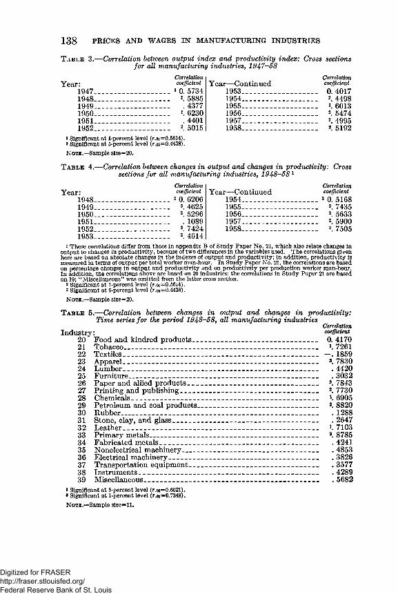
1 3 8 P R IC E S A N D W A G E S I N M A N U F A C T U R IN G IN D U S T R IE S
Table 3.— Correlation between output index and productivity index: Cross sections for all manufacturing industries, 1947-58
Year: Correlationcoefficient Y ear— Continued Correlation
coefficient1947__________________ 1 0. 5734 1953_______________ 0. 40171948__________________ K 5885 1954_______________ 2. 44981949__________________ . 4377 1955_______________ K 60131950__________________ K 6230 1956_______________ 2. 54741951__________________ . 4401 1957_______________ 2. 49951952__________________ 2. 5015 1958_______________ 2. 5192
i Significant at 1-percent level (r.oi= * Significant at 5-percent level (r.os5
=0.5614).=0.4438).
N o t e .—Sample size= 2 0 .
T able 4.— Correlation between changes in output and changes in productivity: Cross sections for all manufacturing industries, 19 4 8 -5 8 1
CorrelationYear— Continued coefficient195 4 3 o. 5168195 5 2. 7435195 6 2, 5 6 3 3
195 7 2. 5900195 8 2. 7505
CorrelationYear: coefficient
194 8 2 0. 6206194 9 3. 4625195 0 3. 5296195 1 . 1089195 2 2. 7424195 3 3. 4614
1 These correlations differ from those in appendix B of Study Paper No. 21, which also relate changes in output to changes in productivity, because of two differences in the variables used. The correlations given here are based on absolute changes in the indexes of output and productivity; in addition, productivity is measured in terms of output per total worker man-hour. In Study Paper No. 21, the correlations are based on percentage changes in output and productivity and on productivity per production worker man-hour. In addition, the correlations above are based on 20 industries; the correlations in Study Paper 21 are based on 19; ‘ ‘Miscellaneous” was omitted from the latter cross section.
2 Significant at 1-percent level (r.oi=0.56i4).3 Significant at 5-percent level (r.oa=0.4438).Note.—Sample size=20.
T a b l e 5.— Correlation between changes in output and changes in productivity: Time series for the period 1948-58 , all manufacturing industries
CorrelationIndustry: coefficient
20 Food and kindred products__________________________________ 0. 417021 Tobacco_____________________________________________________ K 726122 Textiles_____________________________________________________ —. 185923 Apparel_____________________________________________________ 2. 783024 Lumber_____________________________ _______ _____ _____ ____ .442025 Furniture___________________________________________________ . 303226 Paper and allied products___________________________________ 2. 784327 Printing and publishing_____________________________________ 2. 773028 Chemicals___________________________________________________ K 690529 Petroleum and coal products_________________________________ 2. 882030 Rubber_____________________________________________________ . 128831 Stone, clay, and glass_______________________________________ . 264732 Leather_____________________________________________________ *. 710333 Primary metals______________________________________________ 2. 878534 Fabricated metals___________________________________________ . 424135 Nonelectrical machinery-------------------------------------------------------- . 485336 Electrical machinery________________________________________ . 382637 Transportation equipment----------------------------------------------------- . 357738 Instruments_________________________________________________ . 428939 Miscellaneous_______________________________________________ . 5682
* Significant at 5-percent level (r.o5=0.6021).* Significant at 1-percent level (r.oi=0.7348).
N o t e .-—Sample size =*11.
Digitized for FRASER http://fraser.stlouisfed.org/ Federal Reserve Bank of St. Louis
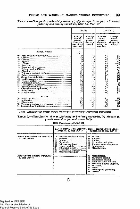
T a b l e 6 .— Changes in productivity compared. yxith changes in output: All manufacturing and mining industries, i $47-53, 1953-57
P R IC E S A N D W A G E S I N M A N U F A C T U R IN G IN D U S T R IE S 139
JL
1947-53 1953-57 '
Average annual percent
change in output per man-hour
Average annual percent
change in output
Average annual percent
change in output per man-hour
Averageannualpercent
change in output
20MANUFACTURING
Food and kindred products..................................... 1H IX
. I
3X 2X21 Tobacco............................ ......... ............................. 4X 2 3X IX22 Textiles.................................................................... 3X IX m“J23 Apparel.................................................................... 1X 2V2 2X
24 Lumber. ................................................................. 4 2 3X -IM25 Furniture............................................................ . IK 3 4H 426 Paper and allied products........................................ % 4 X 3X 4X27 Printing and publishing.......................................... 3 2 428 Chemicals................................................................ 5X 8X 5X 6X29 Petroleum and coal products................................... 3 H 4H 3 IX30 Rubber.................................................................... 2 X 3 2X IX31 Stone, clay, and glass.............................................. 2Vs 4X 3 3X32 Leather.................................................................... m - X 3X 2X33 Primary metals........................................................ 2 H 4 IX 034 Fabricated metals................................................... l M 4 x X X35 Nonelectrical machinery.......................................... 2% 5 - X - X36 Electrical machinery............................................... m 9 X 3X 337 Transportation equipment...................................... 3% i m 5 3X38 Instruments............................................................. 3 X 7X 3% 3X39 Miscellaneous.......................................................... 3 4X m 4
10MINING
Metal mining....... ......... .......................... - ............. l H 2X 4 3%11 Anthracite.............................................—............... - H - i m U X - 2X12 Bituminous................ - ........................................... ZV2 - m 6X 2X13 Petroleum and gas............................. ....... ............. IX X 2%14 Stone and earth minerals______________ _______ 4 X 5X 6H
N o te .—A nnual average percent changes are base year to term inal year compound growth rates.
T able 7.— Classification of manufacturing and mining industries, by changes in growth rates of output and productivity
[1953-57 compared with 1947-53]
Rate of growth of productivity lower 1953-57 than 1947-53
Rate of growth of productivity Higher 1953-57 than 1947-53
Rate of growth of output lower 1953- 57 than 1947-53.
13 Petroleum and gas mining- . 21 Tobacco__________________22 Textiles.23 Apparel.30 Rubber.31 Stone, clay, and glass.37 Transportation equipment.38 Instruments.39 Miscellaneous.
24 Lumber__________________28 Chemicals________________29 Petroleum and coal________33 Primary metals______ —___34 Fabricated metals.................35 Nonelectrical machinery___36 Electrical machinery_______
Rate of growth of output higher 1953- 57 than 1947-53.
10 Metal mining.11 Anthracite mining.12 Bituminous mining.13 Stone and earth minerals.20 Food and kindred products.25 Furniture.26 Paper.27 Printing and publishing.32 Leather.
O
Digitized for FRASER http://fraser.stlouisfed.org/ Federal Reserve Bank of St. Louis