STUDY ON IRRIGATION WATER MANAGEMENT IN … · K. Innocent MUNYENTWARI. iii ABSTRACT ... l ˇefficacitØ de distribution d ˇeau d’irrigation et de la dØtermination le dØbit de

REPUBLIC OF RWANDA

MINISTRY OF EDUCATION

HIGHER INSTITUTE OFAGRICULTURE AND ANIMAL HUSBANDRY (I.S.A.E)

FACULTY OF AGRICULTURAL ENGINEERING AND ENVIRONMENTALSCIENCES

DEPARTMENT OF SOIL AND WATER MANAGEMENT

Presented by:

K. Innocent MUNYENTWARI

For fulfilment for the requirement of the

Bachelor's degree (Ao)

Option: Irrigation and Drainage

Research Supervisor:

Er. SURESH Kumar Pande (M. Tech),

Busogo, December 2011

STUDY ON IRRIGATION WATER

MANAGEMENT IN BASE I SWAMP

RUHANGO DISTRICT

REPUBLIC OF RWANDA





Presented by:










RUHANGO DISTRICT

REPUBLIC OF RWANDA





Presented by:










RUHANGO DISTRICT

i

DEDICATION

To my Parents;

To brothers and sisters;

To all classmates and friends

ii

ACKNOWLEDGEMENT

First and foremost, I thank the almighty God for his abundant blessings and protection during my

field work.

I feel highly indebted to Dr. Charles KAREMANGINGO, the Rector of Higher Institute of

Agriculture and Animal Husbandry, ISAE-Busogo for making excellent environment for

pursuing our studies in the institute.

I am grateful to Professor Dr. SANKARANARAYANAN, Dean, faculty of Agricultural

engineering and environmental sciences for his permission to take up my project research.

My deep sense of gratitude is due to Mr. Suresh Kumar Pande, Head department of Soil and

Water management at the same time my research supervisor for his valuable guidance,

collaboration and constructive suggestion, encouragement and his dedication which helped me to

come to the successful completion of this project work.

I offer my sincere gratitude to all academic staff of the Department of Soil and Water

management. I am grateful to my class mates and all well wishers who helped me to conduct

some of my activities. My heartfelt thanks goes to my dear parents, aunt Floride CYIZA,

colleagues and friends who have shown great understanding and sympathy while I have been

involved in the preparation of this study report.


iii

ABSTRACT

Because of increasing population on the earth it has become inevitable to enhance agricultural

food production on limited land resources. Water is one of the most important inputs for crop

production. Irrigation has been found the best option to cope with the climatic vagaries affecting

mankind for food security. In the process of irrigation, water is lost during storage, conveyance,

application and for accomplishing special needs of plots being irrigated. Identifying the various

components/ways of water losses and knowing what improvements can be made is essential for

making the most effective use of irrigation water.

Therefore a study was undertaken in Base I swamp in Ruhango district with the objectives of

evaluation of irrigation water distribution efficiency and determination of design discharge for

main and secondary canal/channel for irrigating rice crop. To assess the above objectives

detailed methodology is developed for carrying out the study.

The study revealed that the soils are highly permeable with 17.1 cm/hr hydraulic conductivity

(rapid class) leading to high water losses. Results also indicated that very low irrigation

efficiency with 18% poses high water losses to the tune of 82%. The required discharge of main

and secondary channel found was 0.152 cumecs and 0.076 cumecs respectively. The desired

cross section of main and secondary channel found was 0.47 sq.m and 0.27 sq.m respectively.

The secondary channel bed width as proposed by the project was more (0.1m) than actually

found due to siltation and weed infestation. However due to problems such as lack of water

during dry season, weeding, siltation, canal erosion, low use of fertilizers etc; farmers are not

able to get more production in whole areas. The production level of rice in the study area is 5.6

tons/ ha. It is evident that to produce 5.6 tons of rice from one hectare land, an amount of 22970

cubic meter water will be required. The total water losses per day in the whole swamp are

estimated as 1680 cubic meter. Therefore the water use efficiency was 0.24 kg/cubic meter. The

7 hectares are subjected to water logging due to low elevation with respect to water level of main

stream during rainy season and water stagnation during rest of the year. This leads to the losses

of cultivated crops. It is clear from the results that there is a need for good water management for

getting the benefits of irrigation in 105 ha of Base I swamp.

iv

RESUME

En raison de la population croissante sur le monde il est devenu inévitable pour augmenter la

production agricole de nourriture sur les ressources de terre limitées. L'eau est l'une des entrées

les plus importantes pour la production agricole. L'irrigation a été trouvée la meilleure option à

faire face aux extravagances climatiques affectant l'humanité pour la sécurité de nourriture.

En cours d'irrigation, l'eau est perdue pendant le stockage, transport, application et pour

accomplir les besoins spéciaux des parcelles de terrain étant irriguées. L'identification des divers

composants / manières des pertes d'eau et savoir quelles améliorations peuvent être apportées est

essentielle pour faire l'utilisation la plus effiicace de l'eau d'irrigation. Par conséquent une étude

a eu lieu dans le marais de Base I dans le District de Ruhango avec les objectifs d'evaluer

l’efficacité de distribution d’eau d'irrigation et de la détermination le débit de conception pour

canal principal et secondaire.

Évaluer la méthodologie détaillée ces objectifs est développée pour effectuer l'étude. L'étude a

indiqué que les sols sont fortement perméables avec la conductivité hydraulique de 17.1 cm/hr

menant à d'énormes pertes d'eau. Les résultats ont également indiqué que l'efficacité très basse

d'irrigation avec 18% pose des pertes d'eau élevées pour un montant de 82%. Le débit

exigé par le canal principal et secondaire était 0.152 m3/s et 0.076 m3/s respectivement. La

section voulus pour les canaux primaires et secondaires était 0.47m2 et 0.27m2 respectivement.

La base du canal primaire et secondaire propose par le projet était de (0.1m) plus grand que

celles qui existent sur terrain. Partant des problèmes tels que la manque de l'eau pendant la saison

sèche, le sarclage, l'envasement, l'érosion de canal, mauvaise utilisation des fertilisants, etc. Les

agriculteurs ne peuvent pas obtenir plus de production dans leur exploitation. Le niveau de

production du riz est 5.6 tonne/ha. Il est évident que pour produire 5.6 tonnes/ha, une quantité de

22970 m3 l'eau est exigée. La quantité total d’eau pérdu par jour est estimé à 1680 mètre cube.

Par conséquent l'efficacité d'utilisation de l'eau s'est avéré 0.24 kg/m3. Les 7 hectares

connaissaient les problèmes d’inondation dans les saisons pluvieuse et de stagnation dans le reste

de l’an. Ce la mène a la perte des cultures. Elle est claire des résultats qu'il y a un besoin de

gestion appropriée de l'eau pour retirer les avantages de l'irrigation dans le marais de Base I.

v

TABLE OF CONTENT

DEDICATION ............................................................................................................................................... i

ACKNOWLEDGEMENT ............................................................................................................................ ii

ABSTRACT................................................................................................................................................. iii

TABLE OF CONTENT ................................................................................................................................ v

LIST OF FIGURES ..................................................................................................................................... ix

LIST OF TABLES ........................................................................................................................................ x

LIST OF APPENDICES .............................................................................................................................. xi

LIST OF ABREVIATIONS ....................................................................................................................... xii

CHAPTER-1 INTRODUCTION .................................................................................................................. 1

I. 1 Problem statement .................................................................................................................................. 1

I. 2 Principal objective .................................................................................................................................. 2

I. 3 Specific objectives .................................................................................................................................. 2

I. 4 Hypotheses.............................................................................................................................................. 2

I.5 Justification of the study .......................................................................................................................... 2

CHAPTER-2 LITERATURE REVIEW ....................................................................................................... 3

2.1 Importance of irrigation .......................................................................................................................... 3

2.2 Harmful effects of over-irrigation........................................................................................................... 3

2.3 Classification of irrigation methods ........................................................................................................ 4

2.4 Irrigation requirement of rice .................................................................................................................. 5

2.4.1 Good water management practices for rice cultivation........................................................................ 5

2.4.3 Land levelling ...................................................................................................................................... 5

2.5 Swamps development in Rwanda ........................................................................................................... 7

2.5.1 Classification of the swamps in Rwanda ............................................................................................. 7

2.5.2 Management and use of swamps ......................................................................................................... 8

vi

2.5.3 Legal aspects of swamps ...................................................................................................................... 8

2.6 Size of the Basin ..................................................................................................................................... 9

2.7 Shape of the Basin .................................................................................................................................. 9

2.8 Elevation of the watershed ....................................................................................................................10

2.9 The type of arrangement of stream channels ........................................................................................10

2.9.1 Order of stream ..................................................................................................................................10

2.9.2 The length of tributaries .....................................................................................................................11

2.9.3 Stream density....................................................................................................................................11

2.9.4 Drainage density ................................................................................................................................11

2.9.5 Other factors.......................................................................................................................................12

2.10 Various formulas to compute the discharge ........................................................................................12

2.11 Movement of water into the soil .........................................................................................................14

2.11.1 Infiltration ........................................................................................................................................14

2.11.3 Measurement of infiltration .............................................................................................................15

2.11.4 Permeability .....................................................................................................................................15

2.12 The technical aspects in irrigation network ........................................................................................16

2.12.1 Irrigation efficiency .........................................................................................................................16

2.12.2 Water requirement of crops..............................................................................................................16

2.12.3 Available Water (AW) .....................................................................................................................17

2.12.4 Project irrigation efficiency .............................................................................................................18

2.12 .4.1 Water Conveyance Efficiency .....................................................................................................18

2.12.4.2 Water Application Efficiency .......................................................................................................19

2.12.5 Efficiency of irrigation practices, water use and operation of irrigation system .............................19

2.12.5.1 Water Storage Efficiency ..............................................................................................................19

2.12.5.2 Water Distribution Efficiency .......................................................................................................20

2.12.5.3 Water Use Efficiency ....................................................................................................................20

vii

2.12.6 Economic (irrigation) efficiency irrigation system ..........................................................................21

CHAPTER-3 MATERIALS AND METHODS .........................................................................................22

3.1 Study zone description ..........................................................................................................................22

3.1.1 Climate ...............................................................................................................................................22

3.1.2 Soil .....................................................................................................................................................22

3.1.3 Crop ...................................................................................................................................................22

3.2 Materials ...............................................................................................................................................23

3.3 Methodology .........................................................................................................................................23

3.3.1 Discharge measurements procedure...................................................................................................23

3.3.2 Estimated irrigation water conveyance efficiency in the perimeter ...................................................24

3.3.3 Hydraulic conductivity tests...............................................................................................................25

3.3.4 Calculation of evapo-transpiration, infiltration, percolation ..............................................................25

3.3.4.1 Water losses at plots level ...............................................................................................................25

3.3.4.2 Irrigation water requirement using cropwat ....................................................................................26

3.3.4.3 Design of irrigation main and secondary canals .............................................................................26

CHAPTER- 4 RESULTS AND DISCUSSION..........................................................................................29

4.1 Crop water requirements .......................................................................................................................29

4.1.1 Monthly climatic data for Base I rice swamp ....................................................................................29

4.1.2 Monthly evapotranspiration ...............................................................................................................30

4.1.3 Crop water requirement and irrigation requirement...........................................................................31

4.2. Hydraulic conductivity.........................................................................................................................32

4.3 Computation of Irrigation Efficiency....................................................................................................34

4.3.1 Measurement of Discharge ................................................................................................................34

4.3.2 Comparison of Project design dimensions and actually found at field for secondary channel ..........35

4.3.2.1 Channel bed width ..........................................................................................................................35

4.3.3 Measurement of flow velocity ...........................................................................................................36

viii

4.3.4 Discharge ...........................................................................................................................................36

4.3.5 Water conveyance efficiency .............................................................................................................37

4.4 Water losses calculation in Base I swamp at plots................................................................................38

4.4.1 Calculation of percolation, infiltration and evapotranspiration .........................................................38

4.4.1.1 Results of water losses calculation of nine plots in Base I swamp. ................................................38

4.4.2 Water use efficiency ..........................................................................................................................39

4.4.3 Determination of discharge for main and secondary channels ..........................................................40

4.5 Design of primary and secondary channel ............................................................................................40

4.5.1 Design of primary channel .................................................................................................................40

4.5.2 Design of secondary channel .............................................................................................................42

CHAPTER-5 CONCLUSION AND RECOMMANDATIONS .................................................................45

REFERENCE..............................................................................................................................................47

APPENDICES ............................................................................................................................................49

ix

LIST OF FIGURES

Figure 1: Levelled and non levelled land ...................................................................................................... 5

Figure 2: Average monthly climatic data for Byimana meteorological station (1979-2009) .....................29

Figure 3: Average monthly ETo for Base I swamp ....................................................................................30

Figure 4: Average monthly rainfall and effective rainfall ..........................................................................31

Figure 5: Crop water requirement and irrigation requirement from June – November ..............................32

Figure 6: Secondary canal bed width variation...........................................................................................35

Figure 7: Economic trapezoidal channel.....................................................................................................41

Figure 8: Primary canal...............................................................................................................................42

Figure 9: Secondary canal...........................................................................................................................44

x

LIST OF TABLES

Table 1: Permeability classes based on hydraulic conductivity of soil. ......................................................16

Table 2: Approximate Available Moisture Holding Capacity of Soils .......................................................17

Table 3: Data collected during the field study ............................................................................................33

Table 4: Secondary channel cross section and wetted area.........................................................................35

Table 5: Average values of flow velocities at three locations of secondary channel ..................................36

Table 6: Discharge in secondary channel ...................................................................................................36

Table 7: Conveyance efficiency..................................................................................................................37

xi

LIST OF APPENDICES

Appendix 1: Crop water requirement from June to November...................................................................49

Appendix 2: Byimana Mean climatic data used as input into Cropwat 8 ...................................................49

Appendix 3: ETo from Byimana mean climatic data using Cropwat 8 ......................................................50

Appendix 4: Rainfall climatic data used in Cropwat 8. ..............................................................................50

Appendix 5: Crop characteristic (rice) ........................................................................................................51

Appendix 6: Crop irrigation scheduling by cropwat ...................................................................................51

Appendix 7: Answer from the farmers of Base I swamp about production (2011) ....................................52

Appendix 8: Ruhango district map .............................................................................................................52

Appendix 9: Climatological data from Byimana meteorological station (1978-2009)...............................53

xii

LIST OF ABREVIATIONS

AAA: Agro Action Allemande

FAO: Food and Agricultural Organization

FC: Field Capacity

GIR: Gross Irrigation Requirement

MINAGRI: Ministère de l’Agriculture et des Resource animal.

NGOs: Non Governmental Organizations

NIR: Net irrigation Requirement

ORSTROM: Office de Recherche Scientifique et Technologique d’outre Mer

CORIBARU: Cooperative des Riziculteurs du Base/ Ruhango

RSSP: Rural Sector Support Project

ZIGAMA CSS: ZIGAMA Credit and Savings Service

1

CHAPTER-1

INTRODUCTION

The agriculture necessitates the optimum and economic use of water in crop production

process. Though water is plentiful on the earth surface, its exploitation and use for

development of agriculture has not been taken into consideration. The area under irrigation in

the world was estimated to only 241.5 Mha and was only 15.98% in the year 1996 (FAO,

1998).

The agriculture production system in Rwanda is characterized by small arable lands, with a

familiar exploitation of 0.8 hectares (TRANSTEC, 2001). In Rwanda, the arable lands are

estimated to 1,380,000 ha (52% of the total lands) for an estimate of about 8.5 millions

population in 2000 year and for a physical density of 325 population/square km

(TRANSTEC,2001).

The swamps occupy the extent of 165,000 ha with only a half cultivable (MINAGRI, 2000).

The irrigation and drainage are applied only for 5992 hectares of development swamp, with

2584 hectares involved in rice cropping (MINAGRI, 2004). Better swamp management will

increase the higher productivity in addition to the hilly cultivation. The government of

Rwanda has been involved in swamp development to enhance the production by providing

the more easily achievable explorable areas in swamps; this is mainly due to irregularity in

rainfall and increase in population growth and to give a guarantee though optimal

productivity of swamps, by better management of irrigation network. Once irrigation not

properly maintained will result in poor production.

The better distribution and management of water in swamp will help in satisfying future food

demands, for that our work in Base I swamp, case study will conduct into: « The study of

water distribution efficiency in Base I rice swamp, Ruhango District ».

I. 1 Problem statement

There is the problem of spatial and temporal distribution of rainfall that has resulted in

soil erosion and moisture stress on agricultural crops; the major cause of low

productivity.

2

Low interest of the farmers to use appropriate agricultural techniques in order to

increase crop production.

In Base I rice swamp; there is poor distribution of water which occurs over the

secondary and primary canals in irrigation system. The northern part of the swamp

gain excess in water while the southern part has a serious deficiency in water and the

problem of water logging.

I. 2 Principal objective

The main objective of this study is the evaluation of current system of irrigation water

distribution and its efficiency in Base I rice swamp and recommendations for proper

management.

I. 3 Specific objectives

The specific objectives of this study are:

To determine the hydraulic conductivity in Base I rice swamp.

To determine irrigation water requirement through cropwat

To determine the irrigation water flow discharge for main and secondary channels

and comparison of cross section (secondary channel) in proposed and actually

implemented.

To determine water losses of the system and irrigation efficiencies.

I. 4 Hypotheses

The following hypotheses are formulated:

Poor water management yields low water use efficiency.

I.5 Justification of the study

To ensure food security in Rwanda it is vital to use its natural resources like land and

water appropriately. Therefore, swamps which are potential source of agricultural

production have to be exploited efficiently. In this regard, Base I swamp was taken to

study irrigation water efficiency. This study would help to know the causes of low

production and present status of water use. Recommendations would help improving land

and water management for sustainable production.

3

CHAPTER-2

LITERATURE REVIEW

2.1 Importance of irrigation

Irrigation is the artificial application of water, with good economic return and no damage to

land and soil, to supplement the natural sources of water to meet the water requirement of

crops (Majumdar, 2004). A crop requires a certain amount of water at some fixed interval

throughout its period of growth. If the water requirement of the crop is met by natural rainfall

during the period of growth, there is no need of irrigation. Crops receive water from natural

sources of water in forms of precipitation, other atmospheric water, ground water and flood

water. Since the amount, frequency and distribution of precipitation which is the principal

source of water for crops are unpredictable, may be insufficient, unevenly distributed,

untimely, and the ground water may be too deep in the soil profile, irrigation becomes

necessary for successful crop growing. Irrigation should, however, be profitable and applied

in times of crop need and in proper amount. Adequate and timely irrigation leads to high

yields. The excess or under irrigation may damage lands and crops. Irrigation applied earlier

to the actual time of crop need results in ineffective irrigation and waste of water, while

delayed irrigation may cause water stress to crops and reduce the yield (Majumdar, 2004).

Irrigation is the key input in crop production. Full benefit of crop production technologies

such as high yielding varieties, fertilizer use, multiple cropping, crop culture and plant

protection measures can be derived only when adequate supply of water is assured on one

hand. High yielding varieties usually have a higher water requirement than ordinary varieties.

The yield potential of these varieties can be fully exploited if an adequate amount of water is

made available, besides other inputs (Gautam and Dastane, 1970). On the other hand,

optimum benefit from irrigation is obtained only when other crop production inputs are

provided and technologies applied. With adequate supply of water and other inputs, crop

production technologies such as multiple cropping can be profitably applied to boost up

growth and yield of crops (Majumdar and Mandal, 1984).

2.2 Harmful effects of over-irrigation

Irrigation is beneficial only when it is properly managed and controlled. Faulty and careless

irrigation does harm to crops and damages lands, besides causing waste of valuable water.

Rice is the exception and it is grown under soil submergence.

4

When plenty of water is available, most of inexperienced irrigation farmers are tempted to

over-irrigate their lands because they assume that with more water, they will get higher yields

without being conscious of the harmful effects. If the water is used judiciously and

scientifically, there would be practically no ill-effects. Therefore, wide knowledge and

experience are required for efficient water management. These following ill-effects can be

effectively reduced and sometimes altogether eliminated by exercising economical and

scientific use of water.

2.3 Classification of irrigation methods

Water management pertains to optimum and efficient use of water for best possible crop

production keeping water losses to the minimum. Serious water losses occur unless it is

properly monitored while irrigating fields. Various methods are adopted to irrigate crops and

the main aim is to store water in the effective root zone uniformly and in maximum quantity

possible ensuring water losses to the minimum. Each method of irrigation has certain

advantages and disadvantages based on certain principles. Factors such as the water supply;

the type of soil; the topography; the land and the crop to be irrigated; socio-economic, health

and environmental aspects, determine the correct method of irrigation to be used. Whatever

the method of irrigation, it is necessary to design the system for the most efficient use of

water by the crop.

According to Majumdar (2004), the common methods of irrigation are broadly grouped

under:

(1) Surface irrigation methods;

(2) Subsurface or sub-irrigation methods;

(3) Overhead or sprinkler irrigation methods;

(4) Drip or trickle irrigation method.

As it is stated above, irrigation is an artificial application of water for creating favorable

conditions for plant growth. The right quantity of water at appropriate time plays an

important role in crop production. The control of water losses during irrigation is an

important aspect to save this priceless commodity. Irrigation water may be applied to crop by

flooding it on the field surface, by applying it beneath the soil surface, by spraying it under

pressure or by applying it in drops.

The surface irrigation method refers to irrigating lands by allowing water to flow over the

soil surface from a supply channel at upper reach of the field (Majumdar, 2004).

5

The subsurface irrigation, also designated as sub-irrigation, involves irrigation to crops by

applying water from beneath the soil surface either by constructing trenches or installing

underground perforated pipe lines or tile lines. The sprinkler irrigation refers to application

of under pressure water to crops in form of spray from above the crops like rain and that is

the reason why it is also called the overhead irrigation. The drip irrigation, also called trickle

irrigation, refers to the application of water at a slow rate drop by drop through perforations

in pipes or nozzles attached to tubes spread over the soil to irrigate a limited area around the

irrigation (Majumdar, 2004).

2.4 Irrigation requirement of rice

2.4.1 Good water management practices for rice cultivation

Worldwide, water for agriculture is getting increasingly scarce. By 2025, 15-20 million

hectares of irrigated rice may suffer water scarcity. Therefore, care must be taken to use

water wisely and reduce water losses from rice fields. A few principles exist to “get the

basics right” for good water management in paddy rice (H. C. Zhang, 2009).

2.4.2 Field channels

In many paddy fields, water flows from one field to another through breaches in the bunds.

Under such conditions, water in an individual field cannot be controlled and field-specific

water management is not possible, construction of channels to convey water to and from each

field, or group of fields, greatly improves the irrigation and drainage of water (H. C. Zhang,

2009).

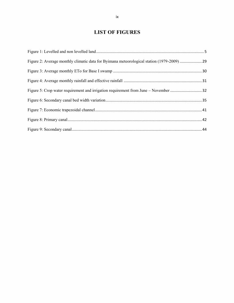
2.4.3 Land levelling

A well-levelled field is a prerequisite for good water management.

When a field is notlevel, water maystagnate in thedepressions whereashigher parts mayfall dry.

source: http://www.knowledgebank.irri.org.

Figure 1: Levelled and non levelled land

Land levelingEffect of uneven fields.

Remedy: land leveling!

http://www.knowledgebank.irri.org

6

Rice is a semi-aquatic plant and hence its water requirements are many times more than most

other food crops with the water requirement of 500 to 2500 mm (T. P. Tuong, 2000). It is,

therefore, a major consumer of the water resources of the country and thus needs careful

water management in order to increase its efficiency of water use. Rice is grown under varied

soil and climatic conditions and its effective root zone depth is 60 cm. Though rice could be

grown on a variety of soils, it grows best on clay loams to clays since these are retentive of

moisture and have low percolation rates of 1-5mm/day (Michael, 1981).

The cultural practices of rice vary widely, depending upon the variety and the local soil and

climatic conditions. However, the condition under which rice is grown could broadly be

grouped into two, namely, low land rice and upland rice. Under low land conditions, rice is

generally transplanted on puddled soils and land is kept under submerged conditions by rain

or irrigation water. The practice of puddling and land submergence, in general, has been

found to reduce the percolation losses, check weed growth, increase the availability of plant

nutrients, regulate soil and water temperature, favour the fixation of atmospheric Nitrogen in

soil through algal growth and improve photosynthesis in the lower leaves due to reflected

light from the water surface (Michael, 1981). The practice of shallow submergence directly

save considerable amount of water as compared to deep submergence.

According to (H. Ikeda and al 2008) the practice of continuous shallow submergence,

however, is possible only when the water supplies are adequate and assured. Land also needs

to be scrupulously leveled to facilitate uniform spreading of water. Weeds, especially the

grassy types, also need to be controlled.

Experimental results are available to show that it is not always necessary to follow the

practice of continuous submergence, especially in the rainy season when the humidity is high

and evaporative demands are low. He also added that under these conditions, the practice of

intermittent submergence, i.e. submergence during the critical stage of initial tillering and/or

flowering and maintenance of saturation to field capacity during the rest of the stages give

yields comparable to those obtain under continuous shallow submergence. The water

supplies, if limited, could safely be curtailed during the non-critical stages of crop growth.

The shortage of water during initial tillering and flowering reduce the yield considerably

while the stages of tillering, grain formation and maturity tolerate water stress to a great

extent (H. Ikeda and al 2008).

7

2.5 Swamps development in Rwanda

The word “swamp” denotes the whole soils of low landscape including humid parts and

marshy soils. Swamps are ecosystems, which have recently caught attention, though the need

for their sustainable development deserves further concern. The importance of swamps is

related to their potential to retain large volumes of water, which can be used for system

maintenance and for dry season agriculture. Agricultural production in Rwanda is extremely

dependent on the rainfall pattern and the climatic uncertainty contributes to wide variations in

crop production. Wherever there are swamps there are people, mainly small farmers and

fishermen. This close association between people and swamps draws attention to the

remarkable strategic importance of these ecosystems in the rural economy and the need for an

effective planning, management and conservation strategy. The arable area is about 825,000

ha, hillside slopes (about 660,000 ha) are not exploited in the dry season and marshlands

(about 165,000 ha) are partially exploited in the rainy seasons depending on their degree of

flooding. About 94,000 ha of marshlands are currently exploited (HYDROPLAN, 2002),

mostly the ones called mineral; whereas the remaining large marshlands made up of peaty or

organic soils covered by Papyrus are not cultivated. However, only 4,000 ha of swamps are

fully equipped with irrigation and drainage systems and 1,200 ha are partially equipped.

2.5.1 Classification of the swamps in Rwanda

According to the Ramsar Convention (1971), the definition of wetlands considers a very wide

range of inland, coastal and marine ecosystems, including lakes, flood plains, freshwater

marshes, estuaries and mangroves (Dungan, 1991).

In Rwanda, semi-detailed characterization and classification studies of swamps have been

carried out. There are different types of classification as follows:

a. Classification according to Cambrezy;

b. Classification according to the size of the swamp;

c. Classification according to the natural vegetation;

d. Classification based on the utilization and stages of the development;

e. Hierarchical classification according to the hydrology.

The hydrology of swamps in Rwanda is basically defined on hydrological conditions which

exist on catchments areas. According to HYDROPLAN (2002), the swamps of Rwanda are

classified in three categories:

8

a. The swamps of high altitude which are in general narrow in shape and under certain

conditions can develop the organic soils in peat. They can be used for water storage, but

in some area they can be used for cultivation. These kinds of swamps are for example

Kamiranzovu and Rugezi swamps.

b. The intermediate swamps or swamps of middle altitude which are often more large in

size. They are essentially situated in Central Plateau.

c. The big swamps of low altitude or collectors swamps which are found in the central

part of Rwanda or along the primary hydrographical network composed by rivers

Nyabarongo, Akanyaru and Akagera.

2.5.2 Management and use of swamps

Water management is the key issue in the use and management of swamps. While drainage is

not so problematic in hydromorphic sandy soils, it can be dangerous in peat soils. Under

improved drained conditions, main cultivated crops are rice, maize, beans and vegetables.

Rice is considered as the main crop to be grown on these soils due to its rooting system which

is well adapted to waterlogged conditions and to its growing cycle during the rainy season,

where the peat soils are likely to be flooded. These soils are, however, quite fragile due to the

absence of the mineral component. Therefore, mismanagement of peat soils can lead to its

degradation and permanent loss for agriculture. The major constraints in the swamps

development are among others the lack of experience and technical skills of farmers to

manage water.

The fragile ecosystem of the swamp to be developed is the major problem of a drastic

decrease of agricultural production. The consequences of those problems are very harmful if

care is not taken by those water users.

2.5.3 Legal aspects of swamps

The necessity to develop legislation on marshlands was perceived very early by the

Government of Rwanda, due to the acuteness of land shortage which characterizes the

country. That situation makes swamps the only alternative to reduce pressure on the fragile

slopes as well as to increase production in order to ensure food security for the population.

In 1988, the Rwandan Government began to work out legislation for the exploitation of

swamps with assistance from various international partners such as FAO.

9

In those legal texts, are defined the status and definition of marshlands, their delimitation,

classification, rules of exploitation, institutions in charge, modalities of management,

maintenance and production, contracts of the utilization of the marshlands, etc. According to

the Organic Law of 14/07/2005 (MINIJUST, 2005) determining the use and management of

land in Rwanda as it is stipulated in Article 14, swamps belong to the State private domain

and can be given to associations/cooperatives or private people according to defined

modalities. However, the uplands are personal or for the family. The social implication of this

fact is that the farmer will give more priority and much care to the uplands than the swamps

which do not belong to him. That is why many swamps are not efficiently and properly

managed.

2.6 Size of the Basin

If the area of the basin is large, total flood flow will take more time to pass the outlet, there

by the base of hydrology of the flood flow will widen out, and consequently reduce the peak

flow because total volume of water passing is the same.

2.7 Shape of the Basin

The shape of the drainage basin also governs the rate at which water enters the stream. The

shale of drainage basin is generally expressed by “Farm factor” and compactness coefficient

as defined below.

Farm factor

The axial length (L) is the distance from outlet to the most remote point on the basin, and

average width (B) is obtained by dividing the area (A) by the axial length.

Compactness coefficient =

If A is the area of the basin and re is the radius of the equivalent circle, then

Circumference = = =2

Therefore, compactness coefficient =

Where P= perimeter of the basin

A= area of the basin

9










managed.








as defined below.

Farm factor









9










managed.








as defined below.

Farm factor









10

There are two types of catchments in general:

Fan shaped catchments

Fern shaped catchments

Fan shaped catchments give greater runoff because tributaries are nearly of the size and

therefore time of flow is nearly the same and is smaller, where as in fern leaf catchments, the

time of concentration is more since the discharge is distributed over a long period.

2.8 Elevation of the watershed

The elevation of the drainage basin, its amount, and hence produce enough effect on the

runoff. The elevation of watershed is a variable factor from point to point in order to

determine the average elevation (Z) of the drainage basin a contour map of the basin is taken

and the Z is then calculated;

Z=

Where, A= area of the basin

A1, A2, A3= area of the area between successive contours

2.9 The type of arrangement of stream channels

If the drainage network of catchment is efficient, water will flow rapidly, and will result in a

higher peak, as the concentration time will be less. Hence the more efficient is drainage, the

more flashy the stream flow will be, and vice-versa. The characteristics of drainage net can

be fairly described by four factors.

Order of stream

The length of tributaries

The stream density

Drainage density

2.9.1 Order of stream

All non branching tributaries, regardless of whether they enter the main stream of its

branches, are termed as first order streams. Stream which receive all non branching

tributaries are on the second order.

10












Z=








Order of stream


The stream density

Drainage density





10












Z=








Order of stream


The stream density

Drainage density





11

Streams of the third order are formed by the junction of two streams of the second order and

so on. In accordance with this system the order number of main stream indicates at once, the

extent of bifurcation of its tributaries is a direct indication of the size and extent of drainage

network.

2.9.2 The length of tributaries

The length of tributaries is an indication of steepness of the drainage basin, as well as of the

degree of drainage. Steep-well drained area generally has numerous small tributaries,

whereas, in plains where soil is deep and permeable, only relatively long tributaries will be in

existence. This factor thus gives the idea of the efficiency of the drainage net. It is generally

better to consider and compare the average length of the same type of tributaries and

especially of first order of tributaries, than to compare the average length of all tributaries.

2.9.3 Stream density

The stream density or stream frequency of a drainage basin may be expressed by relating the

number of stream to the area drained. If Ns is the number of streams in the basin and A is

total area, the stream density Ds can then be expressed as:

D=

ie: The number of stream per km2 in determining the total number of stream, only the

perennial and intermitted streams are included. This factor does not provide a true measure of

drainage efficiency, because a basin having two smaller streams draining only a part of the

basin, and other basin will be indicated to be equally efficient by this factor, whereas it will

not be so, the second being certainly more efficient than the first.

2.9.4 Drainage density

The drainage density is expressed as the length of streams per unit of area. Let Dd represent

the drainage density

L: the total length of perennial and intermittent stream in the basin, and A the area, then:

Dd =

Drainage density varies inversely with the length of overland flow, and therefore provides at

least some indication of drainage efficiency of the basin.

11




network.












D=










Dd =



11




network.












D=










Dd =



12

2.9.5 Other factors

Beside these four important characteristics of drainage basin other factors such as, the soil in

the catchment, land uses at the various factors influence the runoff.

2.10 Various formulas to compute the discharge

The peak flow can be determined either by rainfall method or statistical method by using a

given frequency rainfall on the basin and determination of peak flow of desired period of

recurrence by means of distribution and analyses the discharges measured on the stream

(Nomand,1978)

Generally, the discharge is shown as the product of channel cross sectional area by the flow

velocity.

Q=V x A

Where, Q = Discharge in m3/s

V =Velocity in m/s

A = Cross sectional area in m2

For the estimation of discharge of the stream or channel, the usual formulas are given below:

a) Manning’s-Stricker formula

It is applicable for uniform flow or with variation, for a permanent regime.

Q = AR2/3S1/2

Where, Q =Discharge expressed in cumecs


R = Hydraulic radius in m

S =Longitudinal slope (channel bed slope in m/m)

n = Manning roughness coefficient

The R is obtained by the relation P = wetted perimeter in m

12

2.9.5 Other factors







(Nomand,1978)


velocity.

Q=V x A


V =Velocity in m/s





Q = AR2/3S1/2







12

2.9.5 Other factors







(Nomand,1978)


velocity.

Q=V x A


V =Velocity in m/s





Q = AR2/3S1/2







13

In practice, it is desirable to use at least three transverse sections. Assume S1, S2, S3, Sn-1, Sn

different section taken and with small variations, the area S of the wetted surface can be

obtained as follow:

S =

Where, 1, 2 ….n are different sections

b) Chezy’s formula

When the flow is turbulent both Chazy and manning Stricker formula are preferable. TheChezy formula is expressed by:

V = C when Q =CS

And V = Average velocity

R =Hydraulic radius

I = Hydraulic gradient, m/m

C=

Source: Ministere francaise de la coopération(1974)

c) Rational formula

It is the commonly used formula in irrigation and drainage. In this formula

Q =

Where, Q= peak flow in m3/sec

C =runoff coefficient

I =rainfall intensity in mm/hr

A =catchment area in hectares

13



obtained as follow:

S =




V = C when Q =CS


R =Hydraulic radius


C=


c) Rational formula


Q =





13



obtained as follow:

S =




V = C when Q =CS


R =Hydraulic radius


C=


c) Rational formula


Q =





14

Orstom formula

Qm = Where, Qm = maximum discharge in cumecs

P = maximum rainfall in meters during 24 hours

K = despondency coefficient

A = area of catchment in m2

Tb = base time in seconds

R = runoff coefficient

Qmax= Qα with α, security coefficient ranged from 1to 2.5(Kalisoni, 2004)

d) Rurangwa formula

Qu = 0.116U0.36 A0.82U-0.03

With, Qu = maximum discharge in m3

U = recurrence period in years

A = catchment area in km2

This formula is recommended for Rwanda. It has been proposed by RURANGWA Eugene

and it is obtained with a correlation of 90% on several catchment areas of Rwanda (Kalisoni,

2004).

2.11 Movement of water into the soil

2.11.1 InfiltrationThe movement of water from the surface into the soil is called infiltration. The infiltration

characteristic of the soil is one of the dominant variables influencing irrigation. Infiltration

rate is a soil characteristic determining the maximum rate at which water can enter the soil

under specific condition including the presence of excess water. It has the dimension of

velocity. The actual rate at which water is entering the soil at any given time is called

infiltration rate. The infiltration rate decreases during irrigation. The rate of decrease is rapid

initially and tends to approach a constant value. Cumulative infiltration is the total quantity

of water entering the soil in a given time (Israelson, 1962).

14

Orstom formula








d) Rurangwa formula

Qu = 0.116U0.36 A0.82U-0.03






2004).










14

Orstom formula








d) Rurangwa formula

Qu = 0.116U0.36 A0.82U-0.03






2004).










15

2.11.2 Factors affecting infiltration rate

The major factors affecting infiltration rate are:

Initial moisture content

Condition of soil surface

Hydraulic conductivity of the soil profile

Texture

Porosity

Degree of swelling of soil colloid and organic matter

Vegetative cover

Duration of irrigation or rainfall

Viscosity of water (Michel,1978)

2.11.3 Measurement of infiltration

Three methods are used for estimating infiltration characteristics of soil are used. They are

the use of cylinder infiltrometers, measurement of subsidence of free water in large basin and

estimation of accumulated infiltration from the water in advance data. The use of cylinder

“infiltrometer” is the most common method.

2.11.4 Permeability

Permeability may be defined as the characteristic of porous medium of its readiness to

transmit a liquid. The equation expressing the flow considers the fluidity of liquid and the

permeability factor called intrinsic permeability.

Only the size and shape of soil particles and pore influence it. Intrinsic permeability is the

same as the hydraulic conductivity expect that it is independent of fluid properties such as

specific weight and viscosity, while the hydraulic conductivity is dependent on the fluid

properties and the change with quality of water.

16

Table 1: Permeability classes based on hydraulic conductivity of soil.

Permeability classes Hydraulic conductivity of soil (cm/hour)

1. Extremely slow <0.0025

2. Very slow 0.0025-0.025

3. Slow 0.025-0.25

4. Moderate 0.25-2.5

5. Rapid 2.5-25.0

6. Very rapid >25.0

Source: Smith and Browning (1975)

2.12 The technical aspects in irrigation network2.12.1 Irrigation efficiency

This is used to evaluate how effectively the available water supply is used to crop production;

water is conveyed through canal system, water courses and channels to crop field.

Irrigation is applied to store water in the effective root zone of soil for use of crops.

A considerable loss occurs after its diversion from sources to its actual use by crops. The

extent of water loss in the process decides the irrigation efficiency. Irrigation efficiency

declines as the water loss increase. A high efficiency of an irrigated project is always

desirable. The efficiency may be estimated for various operations beginning from diversion

of water to its actual use, by crops, uniformity in its distribution in the root zone, its use for

crop productivity economics and so on (H. C. Zhang,2009). The methods of estimating,

factors influencing efficiencies and measure to attain a high level of efficiency are discussed

in this study.

2.12.2 Water requirement of crops

Water requirement of a crop refers to the amount of water required to raise a successful crop

in a given period (Majumdar, 2004).

17

It comprises the water lost as evaporation from crop field, water transpired and metabolically

used by crop plants, water lost during application which is economically unavoidable and the

water used for special operations such as land preparation, puddling of soil, salt leaching and

so on. The water requirement is usually expressed as the surface depth of water in

millimeters or centimeters. Crop water requirement may be mathematically formulated as:

CWR = ET + Wm + Wu + Ws or

CWR = CU + Wu + Ws

Where, CWR = Crop water requirement, cm;

ET = Evapo-transpiration from crop field, cm;

Wm = Water metabolically used by crop plants to make their body weight, cm;

Wu = Economically unavoidable water losses during application, cm;

Ws = Water applied for special operations, cm and

CU = (ET + Wm) is the consumptive use of water by the crop, cm.

2.12.3 Available Water (AW)

The available water is defined as the difference between the moisture content of a soil at the

field capacity (FC), and its moisture content at the permanent wilting point (WP) and it is

usually expressed in millimetres.

These quantities are often described as constants, but this is misleading, because they are only

constant for a given soil, and vary with the texture and composition of the soil. The table 2

gives typical values for the soil moisture.

Table 2: Approximate Available Moisture Holding Capacity of Soils

Soil texture Available water(cm/m depth)

Coarse texture-oarse sands, fine sands, loamy sands. 6 – 10Moderately coarse texture - sandy loams and fine sandy loams. 10 – 14Medium texture - very fine sandy loams, loams, and silt loams. 12 – 19Moderately fine texture - clay loams, silty loams, and sandy clayloams.

14 – 20

Fine texture - sandy clays, silty clays, and clays. 13 – 20

Source: Michael and Ojha (1966)

18

2.12.4 Project irrigation efficiency

Irrigation efficiency is usually expressed as the percentage ratio of the amount of water stored

in crop root zone for crop use in the project command area to the amount of water diverted

from the project source (Majumdar, 2004). It is expressed as,

Ep = 100 , Where, Ep = Project irrigation efficiency in percent;

Ws = Amount of water stored in crop root zone soil;

Wd = Amount of water diverted or pumped from the source.

It evaluates the efficiency of an irrigation project and combines the various component

efficiencies. Improvement of irrigation efficiency is achieved by reducing the water loss that

occurs in various ways during water conveyance and irrigation practices. Principal factors

influencing loss and irrigation efficiencies are design and nature of construction of the water

conveyance system, types of soil, and extent of land preparation and grading, design of the

field, choice of irrigation, choice of irrigation methods and skills of irrigations.

Water is loss through evaporation from water surface in conveyance and distribution system

and crop fields during irrigation, through seepage from conveyance and distribution systems

and through deep percolation in crop field. Also water loss through evaporation occurs during

sprinkler irrigation. Sometimes water is loss by runoff from the field due to negligence of an

irrigator. Irrigation efficiency usually varies from 40 to 70%.

2.12 .4.1 Water Conveyance EfficiencyAs already stated, water is conveyed through canal network, water courses and channels from

sources such as reservoirs, rivers and dams to fields or farms for crop use. Conveyance

efficiency is used to evaluate the efficiency of channels conveying water. It is also used to

measure the efficiency of channels conveying water from wells and ponds to field.

Water conveyance efficiency may be defined as the percentage ratio of the amount of water

delivered to fields or farms to the amount of water diverted from sources.

It is expressed as,

Ec = 100 ,

Where, Ec = Water conveyance efficiency in percent;

Wf = Amount of water delivered to fields or farms (at the head of field supply

channel or farm distribution system);

Wd = Amount of water diverted from sources.

18

























It is expressed as,

Ec = 100 ,





18

























It is expressed as,

Ec = 100 ,





19

2.12.4.2 Water Application EfficiencyWater application system refers to the efficiency of water application to field, water is

applied to fields by various methods, and those may be:

a) Surface

b) Subsurface

c) Sprinkler or drip methods

The efficiency of those methods individually or for single irrigation of farm fields may be

estimated. The water application efficiency may be defined as the percentage ratio of the

amount of water stored in the crop root zone to the amount of water delivered to fields. It is

expressed as,

Ea = 100 ( )

Where, Ea = Water application efficiency in percent;

Ws = Amount of water stored in the crop root zone soil;

Wf = Amount of water delivered to fields (Bartsnellen. W, 1997).

2.12.5 Efficiency of irrigation practices, water use and operation of irrigation system

Irrigation practices differ from place to place because of physiographic conditions, soil types,

crop grown, and amount of water available and considerations of farmers. An evaluation of

various irrigation practices and water use by crop is essential to have an insight into the

effective use of available water. The following efficiencies are frequently studied:

a) water storage efficiency

b) water distribution efficiency

c) water use efficiency

2.12.5.1 Water Storage Efficiency

Water storage efficiency refers to the percentage ratio of the amount of water stored in

effective root zone soil to the amount of water needed to make up the soil water depleted in

crop root zone prior to irrigation (Majumdar, 2004). It may be expressed as,

Es = 100 ( ) where

Es = Water storage efficiency in percent;

Ws = Amount of water actually stored in root zone soil from the water applied;

We = Amount of water needed to meet the soil water depleted in the crop root zone soil prior

to irrigation.

19



a) Surface

b) Subsurface





expressed as,

Ea = 100 ( )
















Es = 100 ( ) where




to irrigation.

19



a) Surface

b) Subsurface





expressed as,

Ea = 100 ( )
















Es = 100 ( ) where




to irrigation.

20

The amount of water needed to be applied through irrigation is equal to the amount of soil

water depleted due to evapo-transpiration, which is described as the net irrigation

requirement.

2.12.5.2 Water Distribution Efficiency

Water distribution efficiency measures the extent to which water is uniformly distributed in

the effective root zone soil along the irrigation run (Majumdar, 2004).

It is described as,

Ed = 100 (1 - )

Where, Ed = Water distribution efficiency in percent;

ȳ = Average numerical deviation in depth of water stored in root zone soil along the

irrigation run from the average depth of water stored during irrigation;

đ = Average depth of water stored during irrigation along the water run.

Water distribution efficiency dictates the permissible lengths of irrigation run. It provides a

measure of efficiency of an irrigation system or method over the other.

2.12.5.3 Water Use Efficiency

Water use efficiency is determined to evaluate the benefits of applied water through

economic crop production. It is very important in crop production and irrigation management.

It is described in the following two ways:

i) Field water use efficiency

This may be defined as the ratio of the amount of economic crop yield to the amount of water

required for crop growing (Majumdar, 2004; Hillel, 1998). It is obtained as follows,

Eu =

Where, Eu = Field water use efficiency expressed in kilogram of economic yield per

Hectare-cm or hectare-mm of water;

Y = Economic crop yield in kilogram per hectare;

WR = Water requirement of the crop in hectare-cm or hectare-mm

20



requirement.




It is described as,

Ed = 100 (1 - )














Eu =





20



requirement.




It is described as,

Ed = 100 (1 - )














Eu =





21

ii) Crop water use efficiency

This may be defined as the ratio of the amount of economic yield of a crop to the

amount of water consumptively used by the crop. It is found out as follows,

ECU (or WUE) =

Where, ECU or WUE = Crop water use efficiency in kilogram of economic yield per hectare-

cm or hectare-mm of water;

Y = Economic yield of crop in kilogram per hectare;

CU = Consumptive use of water in hectare-cm or hectare-mm;

ET = Evapo-transpiration in hectare-cm or hectare-mm.

2.12.6 Economic (irrigation) efficiency irrigation system

Irrigation efficiency is the ratio of actual income (net or gross) attained with the operating

irrigation system, compared with the income expected under ideal conditions. This parameter

is a measure of overall efficiency, because it relates the final return to input cost.

i) Operational efficiency

Operation efficiency is the ratio of actual project efficiency compared with the operational

efficiency of an ideally designed and managed system using the same irrigation method and

facilities. Low operation efficiency shows management or system design problems or both.

ii) Water utilization methods

The water utilisation method should provide a high level of water application efficiency and

also ensure its economic viability, sustained soil productivity and wide adaptability to

prevalent features on the farm. Efficiency water application requires careful attention to all

the factors like:

Quality and quantity of water available

Soil characteristics

Topography of the land

The nature and availability of labour and energy

Economic status of the farmer

21




ECU (or WUE) =


















the factors like:






21




ECU (or WUE) =


















the factors like:






22

CHAPTER-3

MATERIALS AND METHODS

To conduct the studies for accomplishing the objectives, certain materials and methods were

used. The details of area, materials used and procedures followed given in the following

paragraphs.

3.1 Study zone description

The Base I swamp is located about 13 km from Muhanga (Gitarama) town falling under

Ruhango District of southern province of Rwanda. The District of Ruhango has sixteen (16)

swamps on a total surface area of 860 ha. However only 417 ha of swamps are well developed for

agricultural activities (Annual report of Ruhango, District, 2010). Since September 2000, the

German Agro-Action has been managing this swamp. The water used to irrigate this swamp

is coming from Base stream and Ruhondo stream. The total area managed is 105 ha. The

Base I swamp is being exploited by the cooperative CORIBARU under control RSSP,

ZIGAMA CSS and Ruhango district. It is a fertile swamp which produces good yield when

well managed.

3.1.1 Climate

Climatological data were collected from Byimana meteorological station (Altitude 1750m,

coordinates 29o44E, 2o25S). Series of long and continue observation of meteorological

parameters rainfall, temperature, Relative humidity, wind and hour of sunshine per day were

gathered from the above station. The appendix 9 presents the climatological data.

3.1.2 Soil

The pedology of the area constitutes the granite and gneiss. The soils of valleys, marshlands

and riversides are alluvial and colluvial. According to (A.A.A, 2005 and Uwitonze T, 2009)

the soil texture of Base I swamp is sandy loam. The soil is fertile and moderately permeable.

3.1.3 Crop

The main crops grown in Base I swamp are rice; however, maize are also grown in some area

of swamp because of various reasons. Before the management of the swamp the crops were

sweet potatoes, beans, soja, irish potatoes and vegetables.

23

3.2 Materials

To determine better ways of irrigation water use management through highly efficient

irrigation, various materials have been used regarding to the tests and measurements to be

conducted

Computer: this device was used for storing and manipulating data;

Measuring tape Stopwatch, A float wooden piece A bucket A wooden post Ruler Calculator Nails

3.3 Methodology

In this work different measurements and tests have been carried out from September to

November, 2011 in order to have a satisfactorily results to determine better ways of water

management in Base I swamp perimeter. The water of Base stream has been diverted through

main irrigation channel which is supplying water to the experimented plots through

secondary channel. The size of each irrigated plot (upper, middle and down sides at both

sides of swamp) is 25m x 40 m.

Briefly the realized measurements/tests are as follows:

1. Discharge measurement received in secondary channel

2. Estimated irrigation water conveyance efficiency

3. Hydraulic conductivity in the field

4. Determination of water losses in the plots.

5. Data processing and analysis with cropwat

3.3.1 Discharge measurements procedure

The velocity of a canal or stream and hence its discharge, may sometimes be determined

approximately by the use of surface floats and its multiplication to cross sectional area of

stream or channel. To use floats a relatively straight reach of a channel 20 metres long with a

fairly uniform cross section along its length is selected (Stern, 1994; Arora, 2004).

24

To reduce the effects of wind on the float, a long-necked bottle partly filled with water was

used as a float. The velocity of the stream is determined by running the float and noting the

time the float takes to cross the channel section. The float is placed in the centre of the

channel 1 or 2 metres upstream of the start of the measured length L, and the time t taken to

cover the measured distance is noted. Three readings are recorded and the mean was taken.

Care is taken to see that the float does not touch the channel sides (USDI, 1953). The distance

divided by the time gives the velocity of the float, which corresponds to the velocity of the

water at its surface.

Length of channel(L) in meter

Water height into channel(D) in meter

Top and Bottom widths of the channel (T) and (B) in meter

Elapsed time (s)

Velocity(V) in m/sec

It has been found that for regular channels flowing in a straight course under favourable

conditions, the mean velocity of a strip in the channel is approximately 0.85 times its surface

velocity for small streams (Stern, 1979; Majumdar, 2004; USDI; 1953). Since the velocity of

water is the highest on the surface, a constant factor equal to 0.85 is used to multiply the

arrived value of velocity to come to the correct value. The formula for estimating the stream

discharge may be written as, Q = 0.85 ( ) D.V, where Q = Discharge, cm3/s; T = Top

width of the channel at flow surface level, cm; B = Bottom width of the channel, cm; D =

Flow depth in the channel, cm and V = Flow velocity, cm/s.

The found discharge were multiplied by 0.85 factor because of weeds availability in channel

with poor roughness

3.3.2 Estimated irrigation water conveyance efficiency in the perimeter

From the water quantity received at the farm gate at the entrance of main channel and the

estimated water delivered to fields, the water conveyance efficiency has been calculated as;

EC = x100

As the cross sectional of the channel was trapezoidal, thus the cross sectional area calculation

was done as:

The area (A) =

Where, T =Top widt B =Bottom width and D = Depth

24












Elapsed time (s)











with poor roughness




EC = x100


was done as:

The area (A) =


24












Elapsed time (s)











with poor roughness




EC = x100


was done as:

The area (A) =


25

3.3.3 Hydraulic conductivity tests

In fact, hydraulic conductivity calculation helped us to know the capacity of saturated soil to

transmit water through it. Reverse auger hole method was used to determine hydraulic

conductivity at field. For this the following process were adopted

Select and level the site;

Dig a hole of 30cm diameter width and 40cm depth;

Collect water to fill the hole using a bucket until is saturated;

Determine initial depth after filling with water;

Using a stopwatch, record a final depth after a certain time internal (5 minutes);

Calculate K using Lewis following formula:

K = 1.15 x r [ ]

Where, K = hydraulic conductivity; cm/sec;

ho = initial depth of water from bottom of hole to water surface, cm;

ht = final depth of water from bottom of hole to water surface, cm;

r = radius, cm;

∆t =time interval; min

3.3.4 Calculation of evapo-transpiration, infiltration, percolation

3.3.4.1 Water losses at plots level

Usually, water consumption is expressed in water depth. Water consumption in depth is

obtained by measuring the change of water level in the paddy field when both water supply

and outflow from the paddy field are controlled. Daily water consumption is defined as water

consumed in the paddy field. For this purpose, the “stake and nail” method has been used for

its easiness and applicability in saturated conditions. Plots for this measurement were

sampled depending on location in the swamp, reliability to inflow and outflow measurement

of water and farmers’ willingness to allow experiments to be conducted in their rice fields.

The sample farm plots were monitored for water losses due to paddy transpiration,

evaporation from standing water in the fields, and lateral and deep percolation.

The procedure is as follows:

25











K = 1.15 x r [ ]




r = radius, cm;














25











K = 1.15 x r [ ]




r = radius, cm;














26

(i) Install a stake on which a nail is attached at exactly the level of the water;

(ii) Close inlet and outlet of water in the plot;

(iii) Measure and record water level and rainfall at a regular time basis;

(iv) Calculate daily change of water level.

The losses through evaporation, evapo-transpiration, percolation and infiltration in the six

plots of rice at a vegetative a stage

H1= initial height of water

H2 = height of water after 24 hours

H3 =height of water after 48 hours

D1T1 = the corresponding time to H1



∆H1 = Difference in water level 1

∆H2= Difference in water level 2

Thus, the total losses =

3.3.4.2 Irrigation water requirement using cropwat

All relevant data have been analyzed mostly using computer software such as Excel to

calculate some parameters needed for discharge calculations and FAO Cropwat 8.0 to

estimate crop water requirements. The following steps were followed for calculation of

irrigation water requirements:

Calculate reference evapotransptraion ETo using FAO CROPWAT Program;

Determine crop coefficient Kc value using FAO-Crop parameters;

Calculate effective rainfall (Pe);

Calculate Net irrigation Requirement (NIR);

3.3.4.3 Design of irrigation main and secondary canals

For this design, Lacey’s theory has been used as method in order to arrive on the design of

irrigation networks.

26




























26




























27

a) Lacey’s theory

Lacey’s theory is based on the concept of regime condition of the channel.

The regime condition will be satisfied if:

The channel flows uniformly in unlimited incoherent alluvium of the same character

which is transported by the channel.

The silt grade and silt charge remains constant

The discharge remains constant

Lacey states that:

“The silt carried by the flowing water is kept in suspension by the vertical component of

eddies”.

The eddied are generated at all the points on the wetted perimeter of the channel section. (N

Basak.2002).

b) Formula used during the design

Lacey’s design equations:

1) drf 76.1 ; where dr = mean dia of silt in mm

2)52 140vAf ; )(&)/( 2mAsmv v velocity ; AreaA

3)6

12

140

Qfv ; smQ /3 Q= discharge

4) QP 75.4 ; )(mP P= wetted perimeter

5) 31

23

4980R

fS &6

1

35

3340Q

fS

6) Regime scour depth:3

1

47.0

fQR ; R=Hydraulic radius or scour depth

7)

63

5

3340 SfQ

S: side slope

28

c) Limitation of Lacey’s theory

Although this theory is used, it has some limitations

1) The concept of true regime is theoretical and cannot be achieve practically;

2) The various equations are delivered by considering the silt factor f which is not

constant at all;

3) The concentration of soil is not taken into account;

4) Silt grade and silt change are not clearly defined;

5) The characteristics of regime channel may not be same for all cases. (K.R.Arora

2004)

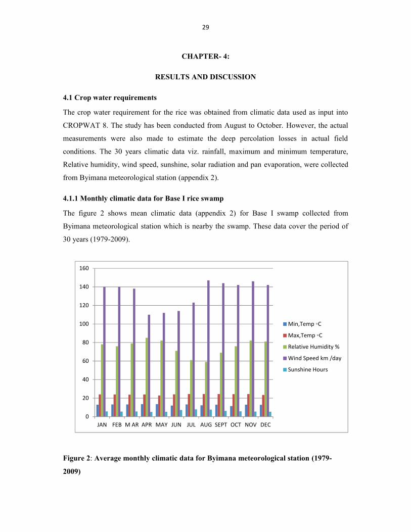
29

CHAPTER- 4:

RESULTS AND DISCUSSION

4.1 Crop water requirements

The crop water requirement for the rice was obtained from climatic data used as input into

CROPWAT 8. The study has been conducted from August to October. However, the actual

measurements were also made to estimate the deep percolation losses in actual field

conditions. The 30 years climatic data viz. rainfall, maximum and minimum temperature,

Relative humidity, wind speed, sunshine, solar radiation and pan evaporation, were collected

from Byimana meteorological station (appendix 2).

4.1.1 Monthly climatic data for Base I rice swamp

The figure 2 shows mean climatic data (appendix 2) for Base I swamp collected from

Byimana meteorological station which is nearby the swamp. These data cover the period of

30 years (1979-2009).

Figure 2: Average monthly climatic data for Byimana meteorological station (1979-

2009)

0

20

40

60

80

100

120

140

160

JAN FEB M AR APR MAY JUN JUL AUG SEPT OCT NOV DEC

Min,Temp ◦C

Max,Temp ◦C

Relative Humidity %

Wind Speed km /day

Sunshine Hours

30

The figure 2 shows that for Base I swamp the average maximum temperature observed over

the period of 30 years ranges from 22.90C to 24.50C with highest during July and August.

However the average minimum temperature ranges from 11.40C to 13.50C with lowest in

October.

The above graph also shows that the minimum humidity is 59% in August and the maximum

humidity is 85 % in April. The minimum wind speed is 110 km/ day in April and the

maximum is 147 km/ day observed in August. The maximum sunshine hour are 7.9 in July

while the minimum sunshine hours are 5.2 recorded in April.

4.1.2 Monthly evapotranspiration

Figure 3: Average monthly ETo for Base I swamp

The figure-3 shows that for Base I swamp; the maximum ETo is 4.02 mm/day in August

followed by September 3.87mm) and July (3.78mm), and the minimum ETo is 3.10 mm/day

in May. As it is shown on the above graphs the high value of ETo are observed during dry

season while the low value are observed during rainy season.

0

0.5

1

1.5

2

2.5

3

3.5

4

4.5

JAN FEB M AR APR MAY JUN JUL AUG SEPT OCT NOV DEC

Eto

(mm

/day

)

Month

Eto mm/day

31

4.1.3 Monthly rainfall and effective rainfall

Figure 4: Average monthly rainfall and effective rainfall

It is evident from figure-4 that maximum rainfall (201 mm) is received during April followed

by May (147mm) and November (136mm) and the minimum rainfall (12mm) is recorded

during July. The maximum effective rain was 136.4mm in April and the minimum is 11.8

mm in July (appendix 4)

4.1.3 Crop water requirement and irrigation requirement

Rice crop was planted from June to November with a total of 180 days (FAO, 2003). ETc

and Irrigation requirements have been determined on decade (10 days) and daily basis. The

figure 5 shows calculated ETc and Irrigation Requirement on decade basis.

31











31











32

Figure 5: Crop water requirement and irrigation requirement from June – November

The figure 5 shows that peak irrigation requirement was 42.8 mm in 3rd decade of July

followed by 37.1 mm in the 1st decade of August, 35.3 mm in 3rd decade of August, 35 mm in

the second decade of August respectively. The lowest irrigation requirement was in1st

(0.7mm) while in 2nd and 3rd decade of November there is no need of irrigation water due to

maturity of crop.

The highest ETc was observed in 3rd decade of August (51.5mm) followed by the 3rd decade

of July, however the irrigation requirement in September was less than the irrigation

requirement of July and August because of the crops’ stage approaching towards maturity

and reduction in crop water requirement and irrigation requirement is reduced. While in July

and August the crop water requirement and irrigation requirement was high because the crop

was in development stage.

4.2. Hydraulic conductivity

Hydraulic conductivity is the permeability of saturated soil. Normally it indicates the

transmission of water in different direction under saturated soil conditions. As rice fields are

mostly having water stagnation, high hydraulic conductivity leads to severe water losses.

Therefore, hydraulic conductivity was determined at Base I swamp by using inverse auger

33

Table 3: Data collected during the field study

K=1.15 x r [ ]

K1= =0.012 cm/sec

K2= = 0.00603 cm/sec

K3= = 0.00402 cm/sec

K4= = 0.0023 cm/sec

K5= = 0.00345 cm/sec

K6= =0.000805 cm/sec

K = = =

K = 0.004768 cm/sec, we say

K = 4.768 x10-3cm/sec

The K measured was 4.768 x10-3cm/sec

S. No Height1(Ho in cm) Height2(Ht in cm) Time (min)1 40 30 52 30 22 53 22 17.5 54 17.5 14.9 55 14.9 12 56 12 11.4 5

33


K=1.15 x r [ ]

K1= =0.012 cm/sec

K2= = 0.00603 cm/sec

K3= = 0.00402 cm/sec

K4= = 0.0023 cm/sec

K5= = 0.00345 cm/sec

K6= =0.000805 cm/sec

K = = =


K = 4.768 x10-3cm/sec



33


K=1.15 x r [ ]

K1= =0.012 cm/sec

K2= = 0.00603 cm/sec

K3= = 0.00402 cm/sec

K4= = 0.0023 cm/sec

K5= = 0.00345 cm/sec

K6= =0.000805 cm/sec

K = = =


K = 4.768 x10-3cm/sec



34

According to the table this shows that the soil on which hydraulic conductivity has been

measured was 4.768 x10-3cm/sec (17.1cm/hr), which means that the soil of Base I is in rapid

class (table-1), very pervious, and care should be taken in order to avoid losses and this

improve puddling operation.

4.3 Computation of Irrigation Efficiency

To determine the conveyance and water application efficiencies field measurements were

done during the study period. The conveyance efficiency was determined in the secondary

irrigation channels covering the whole area under developed swamp.

4.3.1 Measurement of Discharge

To measure the discharge, area- velocity method was used. In this method, measurement of

cross sectional area of selected channel and flow velocity is done. To know the design cross

section and velocities, The Agro Action Allemande document was also consulted and

compared with the actual field conditions. As both channels are not used at a same time,

measurements were taken at one channel and calculations were made. The measurements of

channel section with three locations were done on secondary channel. The following table

indicate the detailed data. It was also found with observation ,project document and

interaction with farmers that both channels on both sides of the swamp are used at the same

time for irrigation and sections of both the channels are of the same size and some parts of the

swamp ridges do not get water because the secondary channels are not well levelled and of

less quantity of water that cannot reach the end of the swamp and that part which do not get

much water is occupied by maize crop.

35

Table 4: Secondary channel cross section and wetted area

Items Projectdesign Section 1 Section 2 Section 3

1 2 3 Av. 1 2 3 Av 1 2 3 AvCanal bedwidth (m)

0.4 0.3 0.2 0.29 0.26 0.3 0.35 0.36 0.34 0.4 0.3 0.23 0.31

Surfacewaterwidth(m)

1 0.56 0.6 0.67 0.61 1 0.6 0.8 0.80 0.8 1.2 0.56 0.85

Top width(m)

1.4 1.9 2 1.8 1.90 1.4 1.4 1.4 1.40 1.4 1.4 1.4 1.40

Ht ofembankment (m)

1.5 1.6 1.7 1.6 1.63 1.5 1.2 1.3 1.33 1.5 1.4 1.5 1.47

Waterheight (m)

0.35 0.32 0.39 0.4 0.37 0.23 0.25 0.26 0.25 0.23 0.25 0.24 0.24

Wettedarea(m2)

0.245 0.14 0.16 0.19 0.16 0.15 0.12 0.15 0.14 0.14 0.19 0.09 0.14

Av.wettedarea (m2)

0.16 0.16 0.14 0.13 0.14 0.12

4.3.2 Comparison of Project design dimensions and actually found at field for secondary

channel

4.3.2.1 Channel bed width

The following graph shows the variation of canal bed width for 3 canal sections

Figure 6: Secondary canal bed width variation

00.05

0.10.15

0.20.25

0.30.35

0.40.45

Section 1 Section 2 Section 3

Comparison beetween Canal bed

actual canal bed (m)

canal bed per agro actionallemande(m)

36

The above figure shows that observed canal bed width was below the designed. This means

that the prevailing problem in selected portions is siltation where transported soil from

catchment area and eroded channel might have raised the channel.

4.3.3 Measurement of flow velocity

The velocity of flow was also measured in all three locations three times at selected channel.

The average values of velocity at each section are presented in the table below.

Table 5: Average values of flow velocities at three locations of secondary channel

Item Location-1 Location-2 Location-3 Average

Length(m) 40 40 40 40

Time(s) 59 64 71 64

Velocity * 0.85(m/s)

0.58 0.53 0.48 0.53

4.3.4 Discharge

The discharge was determined by the multiplication of Average cross section and velocity of

flow at each location. The details are as follows:

Table 6: Discharge in secondary channel

Cross Sectional area

Sq. M

Velocity (m/sec) Discharge (m3/sec)

Location-1 0.16 0.58 0.093

Location-2 0.142 0.53 0.075

Location-3 0.139 0.48 0.067

Average discharge 0.078

37

4.3.5 Water conveyance efficiency

The difference of discharge in three locations is different due to losses on its way. The water

conveyance efficiency is the ratio of water diverted from source to water reached at plot.

Conveyance efficiency is:

Ec=100

Where:

Wf= Amount of water delivered to the fields (at head of field supply channel or farmdistribution system)

Wd= Amount of water diverted from sources

Therefore the observed conveyance efficiencies between first and third locations in the

channel can be taken as conveyance efficiency.

Table 7: Conveyance efficiency

Location Discharge

(m3/sec)

Conveyance Efficiency = (Discharge at

location 2/Discharge at location1) x 100

Location-1 0.093

Location-3 0.067 72%

From the above results, it is evident that due to losses, water conveyance efficiencies are

reduced. The measurements show that the loss of 28% is found. According to Majumdar

(2004), the losses may vary from 25 to 60 percent of water diverted for irrigation. He also

added that in the unlined canals, water ways and channels, the water loss is usually heavy and

the same is attributed mainly to seepage. In fact, growth of undesirable vegetation along and

in canals and in channel beds and sides is also responsible for additional losses.

In addition to that, there were many cracks in channel beds and bunds which may lead to

water losses by seepage. In fact, the canals are not well maintained.

37





Ec=100

Where:






Location Discharge

(m3/sec)



Location-1 0.093










37





Ec=100

Where:






Location Discharge

(m3/sec)



Location-1 0.093










38

4.4 Water losses calculation in Base I swamp at plots

4.4.1 Calculation of percolation, infiltration and evapotranspiration

4.4.1.1 Results of water losses calculation of nine plots in Base I swamp.

Plot H1 (cm) Day I, H2 (cm) Day II, ∆H1 (cm) Day III, H3 (cm) ∆H2 (cm)

1 8.1 9h30a.m 6.3 9h30a.m 1.8 9h30a.m 5.5 1.72 6.8 9h30a.m 5.2 9h30a.m 1.6 9h30a.m 4.6 1.63 9.0 9h30a.m 7.5 9h30a.m 1.5 9h30a.m 6.6 1.94 7.0 9h30a.m 5.1 9h30a.m 1.9 9h30a.m 4.5 1.65 8.7 9h30a.m 7.2 9h30a.m 1.5 9h30a.m 6.4 1.86 9.2 9h30a.m 7.5 9h30a.m 1.7 9h30a.m 6.8 1.77 9.0 9h30a.m 7.0 9h30a.m 2.0 9h30a.m 6.1 0.98 10 9h30a.m 8,0 9h30a.m 2.4 9h30a.m 6.7 1.39 7.8 9h30a.m 6.4 9h30a.m 1.4 9h30a.m 5.9 0.5

D: Day; T: Time; ΔH: Water level difference

Total water losses for nine plots = (1.8 + 1.6+ 1.5+ 1.9 + 1.5 +1.7+2.0+2.4+1.4+ 1.7 + 1.6 +

1.9 + 1.6 + 1.8+1.7+0.9+1.3+0.5) cm

Total losses for nine plots are equivalent to 28.8 cm.

Average water losses per plot = 28.8/9 cm = 3.2 cm/plot/2 days = 3.2 cm/1000 m2/ 2days.

Daily average water losses = 3.2/2 = 1.6 cm/day.

The average water depth maintained was equal to (8.1+6.8+9.0+7.0+8.7+9.2+9.0+10+7.8)/9

= 8.4cm.

The average water losses in the field through ETO and deep percolation are 1.6 cm/day.

The average losses through ETO from Appendix 3 are 737.1 mm/180 days which equal to

average ETO of 4.09 mm/day. The average water losses including ETO and deep percolation

are 1.6cm/day.

Therefore, considering the depletion of water from root zone as 4.09 mm/day, then the total

water applied to compensate water depletion from root zone and deep percolation would be

16.0 mm. Hence loss due to deep percolation = 16 – 4.09 = 11.91 mm say 12 mm

Hence, water application efficiency Ea = 4.09 x 100/16 = 25.56% say 25.6%

The overall efficiency would be Ec x Ea

= 0.70 x 0.256 x 100 = 17.92% say 18%

39

In fact, the deep percolation loss in wet rice is exceptionally high and ranges from 38.3% to

as much as 80% of the water applied in various soils (Mandal and Majumdar, 1983).

Considering gross irrigation (700.2mm) while net irrigation (490.1mm) determined from

cropwat it is clear that 70% irrigation efficiency has been considered. However actual

measurement of irrigation efficiency shows only 18% and actual irrigation requirement

would be 413.6 mm/0.18 = 2297 mm.

4.4.2 Water use efficiency

The average production level of rice in Base I swamp is 5.6 tons/ha (Apendix 7). It is evident

that to produce 5.6 tons of rice from one hectare, an amount of 22970 m3water will be

required. Therefore the water use efficiency would be 5600 kg/22970 m3= 0.24 kg/ m3This

means, to produce 1kg of rice 4.16 m3of water is required.

In Base I swamp, the water application is very poor and it shows that the area under crops is

less due to huge water losses. There is lack of knowledge of farmers in rice water

requirement and its management. The type of soil with high hydraulic conductivity (17.1

cm/hr) and low level of puddling and levelling is the main cause of lower efficiency.

Therefore, the farmers have to manage well the small amount of water received in their rice

fields by uniformly applying it and preventing the deep percolation and run-off losses. The

efficiency may be very low in a badly managed farm and higher in a well managed farm.

Majumdar (2004) stated that the application efficiency can be increased to approach 80% if

crops are under-irrigated by applying lower amount of water than needed because of water

scarcity or high-priced water.

Under-irrigation may completely prevent deep percolation and run-off of water, but it is

undesirable as crops suffer from water stress and give lower yields. Proper land levelling and

grading is a good manner (way) for efficient water application. This is needed to avoid

accumulation of excess water in lower spots leading to deep percolation loss and under-

irrigation of higher spots, and to achieve uniform run and distribution of water in the field.

40

4.4.3 Determination of discharge for main and secondary channels

The peak irrigation requirement found through cropwat was 4.3 mm. considering 18%

efficiency the gross amount of discharge for irrigation can be determined as follows:

Gross irrigation requirement =Net irrigation requirement in m x Area in sq.m/ overall

efficiency;

= 4.3 x10 -3 x 105 (ha) x 10000/0.82 = 5506 cum.

Assuming that irrigation will be supplied for 10 hours;

Hence discharge of main channel would be

5506/(10 x 3600) = 0.152 cumecs

As there are two secondary channels one channel will handle 0.152 cumecs/2 = 0.076 cumecs

4.5 Design of primary and secondary channel

4.5.1 Design of primary channelPrimary canal which take water from intake and divert it in secondary channel, these canalsare located around the edge of the swamp.

Q= 0.152 cumecs

Side slope=1.5:1

As the soil is sandy loam then df; mean particle size df =0.32 because the coarse silt is taken

as standard silt (K.R.Arora,2004).

Silt factor f=1.76df= 1.760.32=0.99 say 1.0

Velocity= 6(0.152x121/40)= 0.32 m/sec

Cross section area = Q/V= 0.152/0.32= 0.475m2

Wetted perimeter= P=4.75Q= 4.750.152=1.85 m

Hydraulic radius=0.47 3Q/f= 0.47 30.152/1= 0.25 m

R = A/P=0.475/1.85= 0.25m

Longitudinal slope:2440

1

152.03340

1

3340 61

35

61

35

Q

fS

During the design of channel, consider the most economical trapezoidal channel section.

41

Figure 7: Economic trapezoidal channel

1) Half top width is equal to side length

T/2 = (b+2my)/2= y1+m2 ( This is the condition for the best side slopes)

m = 1.5

2) tanӨ = 1/m or arctan1/m= Ө and then Ө=340 made to the horizontal. The geometric

elements for the most economical trapezoidal channel section are:

A=(b+my)y

P=2(b+my)

R=y/2

T/2=(b+2my)/2= y1+m2

tanӨ=1/m

A=0.475=(b+my)y=0.475=(b+1.5y)y

{b+(2x1.5y) }/2=y1+1.52

or (b+3y)=3.6y

b=0.6y

P=2(b+my)

1.85=2(0.6y+1.5y)

1.85=4.2y

y=1.85/4.2=0.44m

If b=0.6y

b=0.6x0.44=0.264m

Then our channel will have the following dimensions:

Depth=0.44m

Bed width: b=0.264m

42

Top width; T=b+2my=0.264+2(1.5x0.44)=1.584m

Figure 8: Primary canal

4.5.2 Design of secondary channel

Secondary and third level canals are excavated with respect of their constant cross section

area. They often have the trapezoidal shape and the side slope vary with the type of soil. The

role of secondary and tertiary canals is to transport water with maximum efficiency to the

place of utilization (fields) (HYDROPLAN, 2002). Secondary canal is small than primary,

the discharge which pass in secondary canal is half to that pass in the primary.

Q=0.152 cumecs /2 = 0.076 cumecs

Side slope=1.5:1

As the soil is sandy loam then df; mean particle size df = 0.32 because the coarse silt is taken

as standard silt (K.R.Arora,2004).

Silt factor f=1.76df= 1.760.32=0.99 say 1.0

Velocity= 6(0.076x12/140)= 0.28 m/sec

Cross section area = Q/V= 0.076/0.28= 0.27m2

Wetted perimeter= P=4.75Q= 4.750.076=1.3 m

Hydaulic radius=0.47 3Q/f= 0.47 30.076/1= 0.199 m say 0.2m

R = A/P=0.475/1.85= 0.2m

Longitudinal slope:2174

1

076.03340

1

3340 61

35

61

35

Q

fS

Our channel will be the most economical one with the following characteristics:

1) Half top width is equal to side length

T/2=(b+2my)/2= y1+m2 ( This is the condition for the best side slopes) and m = 1.5

43

2) tanӨ=1/m or arctan1/m= Ө and then Ө=340 made to the horizontal. Ther geometric

elements for a most economical trapezoidal channel section are:

A= (b+my)y

P= 2(b+my)

R= y/2

T/2= (b+2my)/2= y1+m2

TanӨ= 1/m

A=0.27= (b+my)y = 0.27=(b+1.5y)y

{b+(2x1.5y) }/2=y1+1.52

Or ( b+3y) = 3.6y

b= 0.6y

P=2(b+my)

1.3 = 2(0.6y+1.5y)

1.3= 4.2y

y = 1.3/4.2= 0.30m

If, b=0.6y

b = 0.6x0.3= 0.2m

44

Then the channel will have the following dimensions:

Depth=0.3m

Bed width: b=0.2m

Top width; T=b+2my=0.264+2(1.5x0.44)=1.1m

Figure 9: Secondary canal

The most economical secondary channel should contain the above values which have the

small dimension compared to the existing dimensions of the channel from the actually design.

45

CHAPTER-5

CONCLUSION AND RECOMMANDATIONS

The methodology as described in chapter 3 was adopted for the present study. The data

collected, analyzed and discussed. It was found that the soils are highly permeable with 17.1

cm/hr hydraulic conductivity (rapid category) leading to enormous water losses. Results also

indicated that very low overall irrigation efficiency with 18% poses high water losses to the

tune of 82 %.

The water use efficiency was 0.24 kg rice /m3 he required discharge of the main and

secondary channel found was 0.152 cumecs and 0.076 cumecs respectively. The desired cross

section of main and secondary channel found was 0.47 sq.m and 0.27 sq.m respectively; this

is more due to low velocity of design. The secondary channel bed width as proposed by the

project was more (0.1m) than actually found due to siltation and weed infestation. However

due to problems such as lack of water during dry season, low use of fertilizers etc, farmers

are not able to get more production in whole areas. Therefore, other crops like beans, maize

and vegetables are also grown in about 41 hectares while the 7 hectares are subjected to water

logging due to low elevation with respect to water level of main stream during rainy season

and water stagnation during rest of the year due to seepage water from adjacent area. This

leads to the losses of cultivated crops. The negative consequence of variable discharge in the

irrigation canal is that water will be available at upstream fields but not available at the tail

end fields caused by poor land levelling. This can provide the conflicts among the farmers of

downstream and upstream side.

With the above conclusions drawn during this study, the following recommendations are

proposed:

Farmers should be organized and sensitized for effective and efficient irrigation water

management;

Capacity building programmes on efficient water and other inputs management must

be organized by the MINAGRI in coordination with the Ministry of Natural Resources,

agricultural research and educational institutions;

Demonstrations for appropriate input management be done regularly.

MINAGRI should promote rice production, processing and marketing should be

established to safeguard the interest of rice growers;

46

Water users’ associations should be responsible for collecting the prescribed water

charges, timely maintenance of infrastructures and management of the irrigation

scheme;

Lining of peripheral canals and regular maintenance of irrigation and drainage

channels and other infrastructures should be done for long time benefits.

Such study should be conducted in Base I in both agricultural season (A&B).

47

REFERENCE

1. Agro-Action Allemande, 2005. Etude d’aménagements hydro-agricoles et de

protection des basins versants pour les marais de Rugeramigozi Amont, Biringanya

Base et Kiryango.

2. Arora, K.R., 2004. Irrigation, Water Power and Water resources engineering,

Standard Publishers distributors, Fourth Ed., New Delhi.

3. Bartstsnellen W, 1997: Exploitation et entretien des réseaux d’irrigation FAO, Rome.

4. Dungan, P.J. 1991. Wetlands Management: a critical issue for conservation in Africa.

In: Proceeding of the SADC Wetlands Conservation Conference for Southern Africa.

Eds. T.Matiza and H.N. Chabwela.

5. FAO, 1994, Irrigation water delivery models.

6. Gautam, O.P. and Dastane, N.G., 1970. Agronomic practices and water-use patterns

for higher crop yields. Agriculture year book-New Vistas in Crop Yields. ICAR, New

Delhi.

7. H. C. Zhang, 2009: Study on cultival science problem of direct-seeded rice. Beijing:

Chinese agricultural science press, (In Chinese).

8. H. Ikeda, A. Kamoshita, J. Yamagishi, M. Ouk, and B. Lor, (2008) Assessment of

management of direct seeded rice production under different water conditions in

Cambodia. Paddy and Water Environment, Vol. 6.

9. HYDROPLAN, 2002. Schéma directeur de l’aménagement des marais, de protection

des basins versants et de la conservation des sols, Kigali.

10. Islaerson, Orson W. And Hensen, VaughE, 1962.Irrigation principales and practices,

John Wiley and Sons. Inc; USA, and topan company Ltd.Japan.

11. KALISONI, J, 2004: Etude de dimensionnement des ouvrages linéaires et de mise en

valeur du marais Runukangoma, ISAE Busogo.

12. Machibya, M. And Makarius, M., 2005. Comparison Assessment of Water Use and

Damage between Modern and Traditional Rice Irrigation Schemes: Case of Usangu

Basin, Tanzania. In: International Journal of Environmental Research and Public

Health, http://www.ijerph.org, MDPI.

13. Majumdar, D.K., 2004. Irrigation Water Management. Principles and Practices,

Prentice-Hall of India Private Limited, New Delhi.

http://www.ijerph.org

48

14. Mandal, A.K. and Majumdar, D.K., 1983. Effect of phasic soil submergence and

saturation on growth and water use in Rice in semi-arid lateritic tract of West Bengal.

15. Michael, A.M. and Ojha, T.P., 1966. Principles of Agricultural Engineering, Vol. II,

Jain Brothers, First Ed., Jaipur, India.

16. Michael, A.M. and Ojha, T.P., 1981. Principles of Agricultural Engineering, Vol. II,

Jain Brothers, First Ed., Jaipur, India.

17. MINAGRI, 2001: Rapport du projet d’amenagement du marais de l’AKAGERA,

Kigali.

18. MINAGRI, 2003: Formation sur organisation, gestion et entretien des périmètres

d’irrigation, Kigali.

19. MINIJUST, 2005. Official Gazette of the republic of Rwanda. Organic Law

determining the use and management of land in Rwanda, Kigali. Rapport provisoire,

Gitarama.

20. Ruhango district, 2010. Rapport annuel sur le developpement.

21. Smith, 1975: Swamplands soil properties in tropical humid regions, Washington D.C.

22. TRANSTEC, 2004, Rapport sur le recensement de la population au niveau national,

MINALOC, Kigali.

23. T. P. Tuong, A. K. Singh, J. D. L. C. Siopongco, and L.J. Wade, Constraints to highyield of dry-seeded rice in the rainy season of a humid tropic environment. PlantProduction Science, Vol. 3, pp. September 164-172, 2000.http://books.irri.org/9789712202193_content.pdf

http://books.irri.org/9789712202193_content.pdf

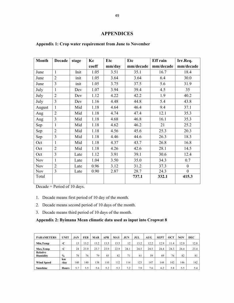
49

APPENDICES

Appendix 1: Crop water requirement from June to November

Month Decade stage Kccoeff

Etcmm/day

Etcmm/decade

Eff rainmm/decade

Irr.Req.mm/decade

June 1 Init 1.05 3.51 35.1 16.7 18.4June 2 init 1.05 3.64 3.64 6.4 30.0June 3 init 1.05 3.75 37.5 5.6 31.9July 1 Dev 1.07 3.94 39.4 4.5 35July 2 Dev 1.12 4.22 42.2 1.9 40.2July 3 Dev 1.16 4.48 44.8 5.4 43.8August 1 Mid 1.18 4.64 46.4 9.4 37.1Aug 2 Mid 1.18 4.74 47.4 12.1 35.3Aug 3 Mid 1.18 4.68 46.8 16.1 35.3Sep 1 Mid 1.18 4.62 46.2 21 25.2Sep 2 Mid 1.18 4.56 45.6 25.3 20.3Sep 3 Mid 1.18 4.46 44.6 26.3 18.3Oct 1 Mid 1.18 4.37 43.7 26.8 16.8Oct 2 Mid 1.18 4.26 42.6 28.1 14.5Oct 3 Late 1.12 3.91 39.1 30.6 12.4Nov 1 Late 1.04 3.50 35.0 34.3 0.7Nov 2 Late 0.96 3.12 31.2 37.3 0Nov 3 Late 0.90 2.87 28.7 24.3 0Total 737.1 332.1 415.3

Decade = Period of 10 days.

1. Decade means first period of 10 day of the month.

2. Decade means second period of 10 days of the month.

3. Decade means third period of 10 days of the month.

Appendix 2: Byimana Mean climatic data used as input into Cropwat 8

PARAMETERS UNIT JAN FEB MAR APR MAY JUN JUL AUG SEPT OCT NOV DEC

Min,Temp ◦C 13 13.2 13.2 13.5 13.5 12 13.2 12.2 12.9 11.4 12.9 12.8

Max,Temp ◦C 24 23.9 23.7 23.9 22.9 24.1 24.5 24.5 24.4 24.3 24.4 23.4RelativeHumidity % 78 76 79 85 82 71 61 59 69 76 82 81

Wind Speedkm/day 140 140 138 110 112 114 123 147 144 142 146 142

Sunshine Hours 5.7 5.5 5.6 5.2 5.3 7.2 7.9 7.6 6.2 5.8 5.5 5.4

50

Appendix 3: ETo from Byimana mean climatic data using Cropwat 8

Appendix 4: Rainfall climatic data used in Cropwat 8.

51

Appendix 5: Crop characteristic (rice)

Appendix 6: Crop irrigation scheduling by cropwat

52

Appendix 7: Answer from the farmers of Base I swamp about production (2011)

S. NAME YIELD/Ha (Tone)A 7.4B 6.5

NORTHERN PART C 7D 6.5E 7.5S.NAME YIELD/HaF 4.8G 4

SOUTHERN PART H 3.5I 5.5J 3.5

Average Production (Tone) 5.62

Appendix 8: Ruhango district map

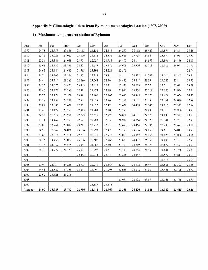
53

Appendix 9: Climatological data from Byimana meteorological station (1978-2009)

1) Maximum temperature; station of Byimana

Date Jan Feb Mar Apr May Jun Jul Aug Sep Oct Nov Dec

1979 24.75 24.858 23.835 23.113 24.132 24.313 24.283 26.112 25.423 24.874 24.84 25.45

1980 25.75 23.025 24.022 23.806 24.512 24.556 23.619 25.954 24.94 23.674 21.96 23.51

1981 23.36 25.346 24.038 23.79 22.929 23.733 24.493 24.1 24.573 23.896 24.186 24.19

1982 23.61 24.532 23.858 23.42 22.683 23.476 24.609 25.506 25.713 26.016 24.07 21.91

1983 24.65 24.644 24.683 21.563 23.396 24.226 23.595 22.94

1984 24.74 23.907 23.396 22.67 22.354 23.31 24 24.538 24.263 23.516 22.363 23.5

1985 24.4 23.514 23.383 22.886 23.264 22.46 24.445 25.248 23.39 24.245 23.1 23.75

1986 24.35 24.075 24.451 23.463 22.412 22.21 22.525 24.009 23.77 23.2 22.69 23.29

1987 23.47 22.772 22.383 22.31 21.974 22.19 21.951 23.974 25.213 24.387 21.976 22.94

1988 23.77 23.178 23.558 23.39 22.406 22.963 23.683 24.848 25.176 24.629 23.056 24.32

1989 23.39 24.357 23.316 22.53 22.038 22.76 23.596 23.141 24.45 24.361 24.036 22.89

1990 23.82 23.085 23.638 22.05 21.822 22.42 21.638 24.438 23.546 24.016 23.323 22.84

1991 23.4 23.472 23.793 22.913 21.703 22.206 23.283 24.99 24.2 22.856 23.97

1992 24.55 25.317 23.996 22.723 22.638 22.776 24.058 24.18 24.773 24.093 23.323 23.5

1993 23.71 24.467 23.79 22.69 22.283 22.55 20.919 24.764 24.123 25.141 23.76 22.83

1997 23.83 23.764 23.012 23.21 22.712 22.5 22.693 23.464 22.796 23.49 23.673 23.18

1998 24.5 22.662 24.038 23.176 22.293 22.42 23.271 23.696 24.053 24.6 24.013 23.93

1999 23.63 23.514 23.506 22.78 22.841 22.913 24.003 24.067 24.466 24.825 23.006 24.06

2000 24.15 24.453 23.022 23.106 22.506 22.766 23.88 24.477 25.156 24.496 23.12 22.93

2001 23.75 24.057 24.525 23.04 21.887 22.306 23.377 24.819 26.176 25.677 24.59 23.59

2002 24.3 24.727 24.151 23.57 22.496 23.5 23.371 24.664 24.93 24.641 23.286 23.57

2003 22.443 22.274 22.64 23.258 24.387 24.577 24.81 23.67

2004 24.916 23.09

2005 23.9 24.03 24.245 22.973 22.271 23.566 22.29 24.532 25.49 23.561 23.393 23.55

2006 24.41 24.327 24.358 23.34 22.09 21.993 22.638 24.048 24.08 23.951 22.776 22.72

2007 23.62 23.621 23.296

2008 23.971 22.822 23.87 24.561 23.756 23.75

2009 23.387 23.473

Average 24.07 23.988 23.762 22.956 22.612 22.969 23.338 24.426 24.581 24.382 23.415 23.46

54

2) Minimum temperature; station of Byimana

Date Jan Feb Mar Apr May Jun Jul Aug Sep Oct Nov Dec1977 12.75 13.155 12.703 13.506 12.996 11.146 10.941 11.312 12.91 12.8 11.31 12.181978 12.69 13.082 13.093 13.086 13 11.516 11.99 12.203 13.33 12.877 13.85 13.5

1979 13.43 12.467 12.612 12.996 13.254 11.75 10.719 12.648 12.6 13.283 12.87 12.64

1980 12.75 12.825 12.416 13.16 14.048 11.473 10.722 9.6064 12.08 12.948 13.06 12.83

1981 13.11 13.262 13.361 13.41 12.593 11.62 10.725 11.761 12.91 12.677 12.29 12.26

1982 12.14 12.685 13.348 13.276 13.058 10.853 10.603 12.387 12.806 13.532 13.1 12.99

1983 12.9 13.578 13.735 13.793 13.219 12.63 12.096 12.041 13.053 12.971 13.28 12.6

1984 12.8 12.717 13.158 13.69 13.806 11.976 11.158 11.516 12.386 13.025 13.01 13.46

1985 13.24 14.158 13.767 14.14 13.516 12.43 12.309 13.08 12.89 13.264 13.21 12.911986 13.24 14.157 13.977 13.626 13.422 11.74 11.496 11.541 13.453 13.177 13.21 13.091987 13.69 13.792 13.883 14.23 13.696 11.1 11.809 12.996 12.863 13.409 12.103 11.251988 11.82 11.5 11.5 11.63 11.838 9.7066 10.554 10.509 11.1 11.245 11.163 10.81989 11.05 11.786 11.312 11.713 11.732 11.42 8.5258 10.786 11.458 11.026 11.21990 11.6 12.025 11.254 11.47 11.803 9.7633 8.8516 10.551 11.686 11.387 11.133 10.381991 10.17 12.228 14 14.176 13.935 13.62 12.961 12.59 12.973 13.577 13.55 12.791992 13.03 13.16 12.783 13.45 13.629 12.263 11.787 12.616 12.946 13.874 13.036 13.061993 13.01 12.624 13.245 12.956 13.793 12 12.161 12.806 13.76 13.88 14.26 13.191997 13.59 14.307 13.98 14.4 14.329 13.35 12.374 12.835 14.413 14.229 14.163 14.171998 14.33 14.289 14.79 14.396 13.971 13.103 12.119 13.025 13.236 13.583 13.13 14.021999 13.65 14.31 13.458 14.536 14.164 12.433 11.483 13.216 13.286 14.18 13.983 13.612000 14.03 13.9 13.377 14.436 14.48 12.616 11.961 12.303 14.056 13.574 13.41 13.822001 13.54 13.575 14.658 14.336 11.896 12.077 13.177 13.013 13.59 13.24 13.352002 13.15 13.153 13.058 13.976 13.89 12.383 11.019 12.8292003 13.82 13.725 11.646 11.206 12.777 13.287 13.526 13.462004 13.577 13.82005 13.44 13.73 14.125 13.613 14.367 13.183 12.067 12.619 13.503 13.174 13.266 13.922006 13.73 14.162 14.122 14.51 13.722 13.463 11.838 12.051 13.536 14.212 13.453 13.412007 13.5 13.557 12.3412008 10.887 13.677 13.246 13.541 13.333 13.452009 12.94 14.887 13.833Averag

e12.94 13.238 13.233 13.551 13.495 12.034 11.35 12.257 12.913 13.197 12.961 12.89

55

3) Rainfall ; station of Byimana

Date Jan Feb Mar Apr May Jun Jul Aug Sep Oct Nov Dec1977 84.6 84.2 145.9 149.2 188.4 6.3 0 30.4 53.3 171.4 233.9 132.91978 112.2 97.6 137.3 273.7 39 1.6 3.5 25.2 52.5 110.2 71.7 45.21979 69.3 121.2 150.4 96.5 99.2 2.1 7 0.8 120.7 144.6 222.2 199.31980 168.5 13.4 130.4 123.1 199.3 15.5 18.4 93.1 104.4 272.4 124.2 131.11981 167.4 99.9 80.2 205.6 402.4 47.5 0 43.8 148.5 33.7 110.8 205.91982 93.3 162.5 106.5 272 68.7 9.9 66 22.1 44.5 134.8 144.6 70.41983 89.7 69 102.4 282.9 141 8 0 42.5 103.7 111.5 146.4 78.11984 30.7 164.5 163 179.8 61.9 22.7 0 100.8 72.2 65.2 136.4 43.71985 40 63 111.3 169.3 293.6 49.4 24 7.8 130 30.9 143.4 193.91986 128.2 171.5 213.8 187.8 91.6 67.8 8.8 0.2 36.7 55.4 170.6 96.11987 88.9 85.7 123.1 121.7 135.4 1.4 0.3 0 65.5 65.3 106.9 44.21988 265.2 152.7 170.9 232 56.3 19.7 17.3 56.2 56.8 103 169.2 64.41989 103.7 132.3 80.8 193.3 197.6 0 16.8 126.6 51.6 42.9 115.2 121.21990 63.3 225.2 68.3 84 103.2 111.5 0 52.2 106.9 223.4 83.31991 85.5 104.2 84 258.9 232.7 4.7 0 36.4 204.8 105.3 189.5 73.11992 76.5 32.6 276.5 173.3 202.4 105.9 87.9 7.8 84.7 34.5 121.7 55.41993 136 82.6 73.9 231.8 142.7 3.4 52.4 14.6 135.2 151.1 92 160.51997 65.1 99.6 113.9 118.5 143.6 31.5 0 82.6 90 94.6 74.3 82.51998 116.3 87.2 105.4 237.4 93.6 7.2 5.5 66.3 119.3 121.7 161.6 109.21999 85.1 125.2 243.1 173 127.8 22 0 39.5 37.1 55.4 106.1 106.92000 210.1 150.3 36.3 185.6 234.7 52.3 0 21.5 5.5 28.8 140.9 129.92001 81.9 96.9 86.2 204.5 160.1 3.8 0 8.9 154.2 110.4 182.9 122.52002 62.2 69.7 150.7 186.9 174.2 0.2 0 148.8 107.5 79.7 62.9 83.42003 68.2 83.3 45.3 247.5 224.6 41.3 0 6.12004 12 200.7 131.4 283.7 70.5 3.3 18.6 36.7 46.4 124.7 177.4 151.42005 78 88 97.5 181.5 26 0.2 65.9 42.2 24.9 171.6 149.1 68.92006 83 126.7 163.7 263.9 65.8 30.6 0 0.2 181.8 116.5 157.9 143.32007 169.6 155.4 128 412.8 183.6 51.2 0 25.1 43.1 145.5 97.5 130.12008 153.1 222.6 111.5 190.5 220.7 87.4 0 32.8 167.7 163.3 344.3 80.82009 90.3 172.3 216.6 218.4 113.1 4.6 0.3 105.4 91.7 97.4 102.9 56.1

Average 110.3 122.72 129.84 201.17 147 30.571 12.456 40.051 84.915 102.95 136.49 108.3

Documents

STUDY ON IRRIGATION WATER MANAGEMENT IN … · K. Innocent MUNYENTWARI. iii ABSTRACT ... l ˇefficacitØ de distribution d ˇeau d’irrigation et de la dØtermination le dØbit de