Study on Ideas on a New National Freight Model System for ...€¦ · carried out an idea study on a new national freight transport model ... goods transport for all modes (road,

RAND Europe

Study on Ideas on a NewNational Freight ModelSystem for Sweden

Gerard de Jong, Hugh Gunn, Warren Walker, Jenny Widell

Prepared for theSAMGODS Group

R

RAND is a nonprofit institution that helps improve policy and decisionmaking through

research and analysis. RAND® is a registered trademark. RAND’s publications do not

necessarily reflect the opinions or policies of its research sponsors.

Published 2002 by RAND

1700 Main Street, P.O. Box 2138, Santa Monica, CA 90407-2138

1200 South Hayes Street, Arlington, VA 22202-5050

201 North Craig Street, Suite 202, Pittsburgh, PA 15213-1516

RAND URL: http://www.rand.org/

To order RAND documents or to obtain additional information, contact Distribution Services:

Telephone: (310) 451-7002; Fax: (310) 451-6915; Email: [email protected]

© Copyright 2002 RAND

All rights reserved. No part of this book may be reproduced in any form by any electronic or

mechanical means (including photocopying, recording, or information storage and retrieval)

without permission in writing from RAND.

ISBN: 0-8330-3327-1

The research described in this report was prepared by RAND Europe and Transek AB for theSAMGODS Group.

RAND Europe and Transek AB Ideas on freight model system for Sweden

November 2001 page II

Preface In a contract for the SAMGODS group, containing the Swedish national road, rail and aviation administrations and led by SIKA, RAND Europe, toigether with Transek has carried out an idea study on a new national freight transport model system for Sweden. The objective of the study was: To provide state-of-the-art ideas that are consistent and innovative on a co nceptual framework for policy orientated analyses and modelling of freight transport in a Swedish context. The new Swedish freight transport model system, that should succeed the present SAMGODS model, should cover all modes (road, rail, air, maritime) and geographic levels (international, national, regional). Furthermore, it should be able to provide medium and long run forecasts (certainly including 10-25 years ahead), and be capable of being used to assess transport policy measures and for the evaluation of infrastructure projects. The SAMGODS group has decided to commission four idea studies, each of which can cover either the full model system or parts of it. This report contains the outcomes of an idea study covering the full model system.


November 2001 page III

Preface........................................................................................................................II

Summary...................................................................................................................IV

1. Introduction...........................................................................................................1

1.1 Background and objectives................................ ................................ .................... 1

1.2 The study team’s interpretation of the study task .................................................. 1

2. Available Information........................................................................................3

2.1 Review of international experience on European, national and regional freight transport models......................................................................................................... 3

2.2 Existing data ....................................................................................................... 12

2.3 The present SAMGODS models and tools........................................................... 17

3. Proposed New Model System for Freight Transport ..............................23

3.1 Basic ideas behind the suggested approach................................ .......................... 23

3.2 The proposed model structure ............................................................................. 24

3.3 Theoretical foundations of the suggested approach ............................................. 34

3.4 The proposed mix of formalised versus non -formalised methods ........................ 34

3.5 Use of existing models and tools, modification or new developments................... 35

3.6 Adaptibility and tentative ideas for further development.................................... 36

4. Development of the New Model System ......................................................38

4.1 Data requirements, use of existing data and proposed new data collection.......... 38

4.2 The estimation and calibration process ............................................................... 40

4.3 The implementation process................................................................................ 41

4.4 The validation process ......................................................................................... 42

4.5 Fall-back options................................................................................................. 42

5. Designing and Using the New Model System ...........................................44

5.1 Introduction ........................................................................................................ 44

5.2 Flexibility, modularity, maintenance, and updating ............................................ 44

5.3 Interactive use by non -computer experts ............................................................. 45

5.4 User initiation and control................................................................................... 46 5.5 Use for practical purposes................................................................................... 46

5.5 Compatibility with existing frameworks and tools............................................... 49

5.6 Using the model in a Nordic context .................................................................... 50

References ................................................................................................................51


November 2001 page IV

Summary This report describes the outcomes of an idea study on a new national freight transport model system for Sweden. The study was carried out by RAND Europe (main contractor) and Transek AB (subcontractor), for the SAMGODS group. The objective of the study is To provide state-of-the-art ideas that are co nsistent and innovative on a conceptual framework for policy orientated analyses and modelling of freight transport in a Swedish context. The new Swedish freight transport model system, that should succeed the present SAMGODS model, should cover all modes (road, rail, air, maritime) and geographic levels (international, national, regional). Furthermore, it should be able to provide medium and long run forecasts (certainly including 10-25 years ahead), and be capable of being used to assess transport policy measures and for the evaluation of infrastructure projects. The SAMGODS group has decided to commission four idea studies, each of which can cover either the full model system or parts of it. This report contains the outcomes of an idea study covering the full model system. We recommend that two different models will be developed: • A fast policy analysis model, for initial screening and comparison of policy

alternatives; • A detailed network-based forecasting model, for predictions at the network level

and to provide inputs for project evaluation. The former model can be a developed as a system dynamics model, which does not only cover freight transport, but also macro-economic development, land use and the environment (but at a rather general level). It can be constructed to be broadly consistent with the sensitivities of the detailed model. For the the detailed model we propose to develop a number of interlinked modules: At the national/international level: • An input-output model for production and attraction and a distribution model; • A disaggregagte model for mode and shipment size choice; At the regional/urban level: • A disagregate model linked with the passenger model SAMPERS; At all geographical levels: • An assignment module.


November 2001 page 1

1. Introduction 1.1 Background and objectives The SAMGODS group has contracted RAND Europe and Transek AB to carry out an idea study on ‘a conceptual framework for analysis and model support for Swedish studies of freight transport and transport policy’. The objective of the idea study is: To provide state-of-the-art ideas that are consistent and innovative on a conceptual framework for policy orientated analyses and modelling of freight transport in a Swedish context The idea study can be regarded as a preliminary study that is part of the preparatory phase preceding the development of a new freight model system. The SAMGODS group has decided to commission a number of such idea studies, each of which can cover either the full model system or parts of it. This report contains the outcomes of the idea study covering the full model system carried out by RAND Europe together with the Swedish transport consultant Transek. RAND Europe was the main contractor; Transek acted as a subcontractor to RAND Europe. 1.2 The study team’s interpretation of the study task The new national model system for freight transport should have the following capabilities: • Providing forecasts (for a reference case and alternative scenarios) of the

development of goods transport for all modes (road, rail, air, maritime) for relevant time periods (certainly including 10-25 years ahead) and at different geographical levels (international, national, regional)

• Supporting analyses of transport policy measures and new infrastructure, including impacts on traffic generation and distribution and on land use and regional employment. The types of applications can range from forecasting the effects of changes in individual (major) links to system-wide analyses.

• Providing input for the evaluation (at present mainly Cost-Benefit Analysis) of transport policy measures and infrastructure projects, including the distribution of benefits and costs (e.g. over sectors, regions and population groups).

The present Swedish national model system for goods transport, the SAMGODS-model, is a set of separate models which have been made to interact by inserting results from one model as inputs or constraints into a next model. SAMGODS has been criticised for the following weaknesses, which will be the focus areas for new developments, but which cannot necessarily all be remedied in a next system version: • Logistic thinking (e.g. link between transport and inventory policy, choice on

shipment size and on number and location of warehouses, consolidation versus distribution, using a commodity classification which is based on logistic requirements) is hardly or not included.

• The model is far from transparent.



• Transport through Sweden is not treated well. • Forecasts in terms of monetary values (Swedish Kronor) are transformed into

forecasts in terms of tonnes for each of the commodity groups. Not much is known about the future values of these value-to-weight transformations, but assumptions about these values have a large impact on the results in tonnes.

• The model validation has been very limited. • The demand matrices are fixed; there is no feedback to generation (production and

attraction) and distribution. • Many policies (e.g. Eurovignet) and new phenomena (e.g. e-commerce) are hard

to represent. • Mode and route choice use the same algorithm (within the STAN software). • Running the model requires considerable knowledge, time and cost. The new freight model could use components of the existing SAMGODS-model. It should relate to the recently developed model for passenger transport (SAMP ERS) and existing or new evaluation tools. At present, SAMPERS and SAMGODS are totally separate models. In STAN, the matrices in tonnes are assigned directly to the networks without a transformation into vehicle units. Assignment of passenger cars takes place separately in the passenger model SAMPERS.



2. Available Information 2.1 Review of international experience on European, national and regional freight transport models 2.1.1 Existing reviews Recent reviews of various types of freight transport models can be found in Cambridge Systematics (1997), Regan and Garrido (2000), Pendyala and Shankar (2000), Chapters 32-34 (by Friesz, D’Este and De Jong respectively) in the handbook edited by Hensher and Button (2000), EXPEDITE (2000) and Willumsen (2001). As part of the SPOTLIGHTS project for DGTREN of the European Commission, a European Model Directory (MDir) has been established, which contains information on 222 transport models in Europe (some double counting has occurred). Sixty-five of those models are freight transport models and 29 are joint passenger and freight transport models (Burgess, 2001). Older reviews, some of which are still quoted regularly, are Gray (1982), Winston (1983), Harker (1985), Zlatoper and Austrian (1989), RTC/HCG/SDG (1991), Oum, Waters and Yong (1992) and Ortuzar and Willumsen (1994, especially Chapter 13). The current review takes into account these existing reviews, but also some additional literature. 2.1.2 Four steps Many modelling concepts applied in freight transport forecasting have originally been developed for passenger transport. Most authors (e.g. Pendyala and Shankar, D’Este) seem to agree that the four-step transport modelling structure from passenger transport can fruitfully be applied to freight transport as well. However within each of the four steps the freight models can be very different from those in passenger transport. Important differences between the freight and passenger transport markets are the diversity of decision-makers in freight (shippers, carriers, intermediaries, drivers, operators), the diversity of the items being transported (from parcel deliveries with many stops to single bulk shipments of hundred thousands of tonnes) and the limited availability of data (especially disaggregate data, partly due to confidentiality reasons). The four steps in the context of a freight transport model system are: 1. Production and attraction. In this step, the quantities of goods to be transported

from the various origin zones and the quantities to be transported to the various destination zones is determined (the marginals of the OD matrix). The output dimension is tonnes of goods. In intermediate stages of the production and attraction models, the dimension could be monetary units (trade flows).

2. Distribution. In this step, the flows in goods transport between origins and

destinations (cells of the OD matrix) are determined. The dimension is tonnes. 3. Modal split. In this step, the allocation of the commodity flows to modes (e.g.

road, train, combined transport, inland waterways) is determined.



4. Assignment. After converting the flows in tonnes to vehicle -units, they can be assigned to networks (mostly this is about assigning truck flows together with passenger cars to road networks).

Besides these four steps, a number of transformation modules are usually required within a comprehensive freight transport model system. Such transformations could involve converting trade flows in money units into physical flows in tonnes to determine production and attraction. This can be done by using value/weight ratios for different commodity groups. The ratios used here may have a large impact on the final predictions and therefore it is important to assemble good data on the conversions and if possible to make it an endogenous, policy sensitive choice within the model system. Another transformation module is that for going from flows in tonnes to vehicle units, such as HGV’s, as might happen between mode choice and assignment. Actually, this is influenced by a great number of decisions on shipment frequency, shipment size, return loads and vehicle utilisation rates. These decisions could be modelled explicitly in additional logistic modules (e.g. in the SMILE model, see Tavasszy et al., 1998), but often fixed conversion rates are used here as well. Another type of transformation module is a regionalisation module to go from a coarse to a fine zoning system. In the remainder of this section on the review of international experience, we shall discuss the types of models developed for each of the four steps and give examples of each of the types. For reasons of space, we shall not describe specific model systems one by one, but limit ourselves to a discussion by type of model. Models integrating several steps (e.g. production, attraction and distribution, or modal split and assignment) will be discussed as well. Models including additional choices (e.g. shipment size, location of distribution centres) will also be included. The focus will be on models at the national level, but models for international and urban flows will be included as well, since these are also required within the new national Swedish freight model system. Models for short-term operational decisions for operators are not covered, since the model system to be developed is for medium- to long-term transport planning and policy formulation. 2.1.3 Models for production and attraction Within this first step we can distinguish three types of models that have been applied in practice: • Trend and time series models • System dynamics models • Zonal trip rate models • Input-output and related models. All these models are based on aggregate data. We have not found examples of production and attraction models in freight transport on disaggregate data. In trend models historical trends are extrapolated into the future. Time series data have been used to develop models of various degrees of sophistication, ranging from simple growth factor models to complex auto-regressive moving average models (e.g.



Garrido, 2000). The latter mode l uses information only on truck flows and is meant for short-term forecasting. Time series models with explanatory variables, such as GDP, have been developed as well. In system dynamics models (e.g. the system of models used in the ASTRA project for the EC), the changes in the transported quantities over time and feedbacks to/from the economy, land use and the environment are modelled explicitly. The parameters of the model system are usually not obtained from statistical estimation, but from existing literature and by trying initial values and checking the resulting dynamic behaviour of the system (trial and error). A system dynamics model might include the distribution and modal split steps as well. System dynamics models, however, usually do not conta in sufficient spatial and network detail to yield zone-to-zone flows and link loadings. Zonal trip rates for production and attraction are usually derived from classifying cross-sectional data on transport volumes to/from each zone in the area under investigation (or another similar area) into a number of homogeneous zone types. Examples of such rates can be found in the Quick Response Freight Manual (Cambridge Systematics et al., 1998) and in the Guidebook on Statewide Travel Forecasting (FHWA, 1999). Input–output models are basically macro-economic models that start from input-output tables. These are tables that describe, in money units, what each sector of the economy (e.g. textile manufacturing) delivers to the other sectors, also including the final demand by consumers, import and export. National input-output tables have been developed for many countries, usually by a central statistical office. A special form of input-output table, which for many countries does not exist, is a multi-regional or spatial input-output table. This not only includes deliveries between sectors, but also between regions (trade flows). Most multi-regional input-output tables distinguish only a few, large regions within a country. The input-output model assumes that for forecasting, the multi-regional input-output table can be scaled up on the basis of predicted sectoral growth. The new input -output table can then give the future trade flows between regions, using either: • Fixed technical and trade coefficients: the present production and trade patterns

are extrapolated into the future. • Elastic technical and trade coefficients: functions are estimated (e.g. multinomial

logit) in which the fraction that is consumed in region i of the production of sector s in region j depends on the total production of region j in sector s and the (generalised) transport cost, in relation to other regions j. This makes generation and distribution sensitive to changes in transport cost and time (a form of induced demand).

Examples of multi-regional input-output models in freight transport are: • The Italian national model system for passengers and freight (Cascetta, 1997),

which uses 17 sectors and 20 regions and also has elastic coefficients.



• The REGARD model for Norway, with 28 sectors, which produces demand used in the Norwegian freight model NEMO (see EXPEDITE, 2000).

• The model for Belgium developed by ADE with 17 sectors, which produces

demand used in the Walloon Region freight model WFTM (Geerts and Jourquin, 2000).

• The SCENES European model system for passengers and freight and its

predecessor STREAMS (Leitham et al, 1999), with 33 sectors and (eventually) more than 200 zones in Europe and elastic coefficients (SCENES Consortium, 2000).

The Dutch model TEM-II (see Tavasszy, 1994) and the present Swedish SAMGODS use a multi-sectoral input-output table for the country as a whole (not multi-regional), which is transformed from money units into tonnes and is regionalised (e.g. on the basis of regional shares in employment and population). The Dutch SMILE model (Tavasszy et al., 1998) does not use input-output tables but uses related ‘make and use’ tables with production and consumption by sector (using 222 sectors). For each commodity class, a production function is developed. As in TEM-II, the analysis takes place at the national level, and is regionalised later. The multi-regional input-output models and the related multi-sectoral economic models (e.g. ISMOD within SAMGODS) used in this first step, can be regarded as computable general equilibrium (CGE) models, establishing equilibrium in several related markets. CGE models in economics (not focussing on transport) often include economic issues that are not handled in transport models, such as type of competition and economies of scale. Just as system dynamics models, input-output models can be used to give transport – land use interactions. A model type that has not been applied in practice is that based on the ‘new trade theory’ (Markusen and Venables, 1998), in which a multi-national plant is studied that chooses the number and location of plants. National and international commodity flows then result from such location decisions. Table 1 summarises the advantages and disadvantages of the four types of models that can be used in ste p 1.



Table 1. Summary of freight transport production and attraction models Type of model Advantages Disadvantages Time series Limited data requirements

(but for many years) Little insight into causality and, limited scope for policy effects

System dynamics Limited data requirements Can give land use interactions External and policy effects variables can be included

No statistical tests on parameter values

Trip rates Limited data requirements (zonal data)

Little insight into causality and limited scope for policy effects

Input-output Link to the economy Can give land use interactions Policy effects if elastic coefficients

Need input-output table, preferably multi-regional Restrictive assumptions if fixed coefficients Need conversion from values to tonnes

2.1.4 Models for distribution As in the previous step, all freight distribution models found in the literature are based on aggregate data. In the distribution module of a freight transport system, the trade flows (in tonnes) between origin zones and destination zones are determined based on measures of production and attraction (usually the outcomes of the step described above) and a measure of transport resistance. The latter is expressed as transport cost or generalised transport cost. The most commonly used method is the gravity model. In such models the flow between zone i and zone j is a function of the product of production and attraction measures of zone i and zone j respectively divided by a some measure of the (generalised) transport cost. Gravity models for distribution in freight are included in: • The Dutch TEM-II model (see Tavasszy, 1994) • The Dutch SMILE model (Tavasszy et al., 1998) • The Great Belt traffic model (Fosgerau, 1996) • The Finnish study on different distribution model types (Iikkanen, et al., 1993). In the Italian national model, the freight OD flows follow from the multi-regional input-output analysis with elastic coefficients (after transformation from money units into tonnes and after regionalisation). In other words, a multi-regional input-output model can supply both production/attraction and distribution. A similar method was used in STREAMS and SCENES. The European freight transport model NEAC (see Chen and Tardieu, 2000) also models distribution simultaneously with production and attraction on the basis of value added per sector and transport cost in a gravity-type model. The Fehmarn Belt freight transport model uses a gravity model for the joint determination of attraction and distribution as well (Fehmarn Belt Traffic Consortium, 1998). Table 2 summarises the advantages and disadvantages of the gravity and input-output models for step 2.



Table 2. Summary of freight transport distribution models Type of model Advantages Disadvantages Gravity Limited data requirements

Some policy effects through transport cost function

Limited scope for including explanatory factors and policy effects Limited number of calibration parameters

Input-output Link to the economy Can give land use interactions Policy effects if elastic coefficients

Need input-output table, preferably multi-regional Restrictive assumptions if fixed coefficients Need conversion from values to tonnes

2.1.5 Models for modal split For modal split for freight, both aggregate and disaggregate (includin g stated preference, SP) models can be found in the literature. The following models for modal split are distinguished: • Elasticity-based models • Aggregate modal split models • Neoclassical economic models • Econometric direct demand models • Disaggregate modal split models (including inventory-based models and models

on SP data) • Micro-simulation approach • Multi-modal network models. Elasticity-based models reflect the effects of changing a single variable (e.g. the cost of some mode). The elasticities are derived from other models or expert knowledge. Such models are mostly used for strategic evaluations and/or for a quick first approximation (followed by more detailed analysis using other model forms) or in situations where data are very scarce. An example in freight is the PACE-FORWARD model (Carrillo, 1996). Aggregate modal split models are mostly binomial or multinomial logit models estimated on data on the shares of different modes for a number of zones. They are meant to give the market share of a mode, not the absolute amount of transport (tonnes) or traffic (vehicles) as the direct demand models do. Consequently the elasticities from such models are conditional elasticities (conditional on the quantity demanded; see Beuthe et al., 2001). The aggregate modal split model can be based on the theory of individual utility maximisation, but only under very restrictive assumptions. A disadvantage of using the multinomial form is that the cross elasticities are equal. Examples are Blauwens and van de Voorde (1988) for inland waterways versus road transport and the modal split model within NEAC.



Neoclassical models start from the economic theory of the firm. For a cost function, with transport services as one of the inputs, a demand function for transport can be derived using Shephards’s Lemma. Examples of estimations of such transport demand functions can be found in Friedlaender and Spady (1980) and Oum (1989). The explanatory variable here is the budget share of some mode in the total cost. This makes it hard to combine these models in a larger (four-step) transport model system, because here the share in the transport volume is the relevant variable. In a direct demand model, the number of trips (or kilometres) by some mode is predicted directly (unlike the market share forms discussed above, which are conditional on an external prediction of total demand over all modes). A classic example is the abstract mode model by Quandt and Baumol (1966). This model is also hard to incorporate in the four-step framework. Disaggregate modal split models use data from surveys of shippers, commodity surveys and/or stated preference surveys. Most of these models are multinomial logit (MNL) or nested logit (NL), which for disaggregate observations can be based on random utility maximisation theory under quite general assumptions. The property of identical cross elasticities found in aggregate modal split models applies in disaggregate MNL models as well, but not in NL. The current proliferation of logit-based functional forms in passenger transport modelling and elsewhere (e.g. error components or mixed logit, see McFadden and Train, 2000) has not had much effect in freight transport modelling yet. Most disaggregate freight models deal with mode choice only. Examples are: • Winston (1981): A probit model for the choice between road and rail transport by

commodity group in the US • Jiang et al. (1999): a nested logit model on the French 1988 shippers survey. • Nuzzolo and Russo (1995): the mode choice model for the Italian national model • Fosgerau (1996): a mode choice model on revealed and stated preference data • Reynaud and Jiang (2000): Eufranet: a European freight model focussing on

operating systems for rail developed for DGTREN with a mode choice model on revealed and stated preference data

• FTC (1998): a mode choice model on revealed and stated preference data • De Jong et al. (2001): a mode choice model on revealed and stated preference data

for the north of France, developed for the French Ministry of Transport. Furthermore there are several models on SP data only, but these are not developed for transport forecasting, but for providing value of time measures (reviewed in Chapter 34 of Hensher and Button, 2000). Some other disaggregate freight transport models simultaneously deal with mode choice and logistic choices (inventory-based models). Disaggregate models in which the mode choice decision is embedded in a larger inventory-theoretic and logistic framework include:



• Chiang et al. (1981) for location of supplier, shipment size and mode choice • McFadden et al. (1985) for shipment size and mode choice • Abdelwahab and Sargious (1992) and Adelwahab (1998) for mode choice and

shipment size (this is a joint discrete-continuous model estimated on the U.S. Commodity Transportation Survey)

• Blauwens et al (2001) for mode choice based on total logistic cost (also including handling and inventory cost).

In the US, a prototype freight transport model has been developed for the Portland region, with an upper level model that produces zone-to-zone flows in money terms (an input –output model) and a lower level model that estimates urban vehicle trip patterns starting from the outputs of the upper level model (Neffendorf, et al., 2001). The lower level model is called a micro-simulation model. This is a tour and trip level model for freight transport by lorry. It includes conversion to shipments, allocation to individual organisations, assignments of transhipment points, allocation to carrier type and vehicle type, generation of tours to get sufficient vehicle loads and conversion of tours to trips for assignment. Many of these steps are carried out by Monte Carlo simulation, but observed data on distributions are used, if available. A similar two-level system has been proposed (Neffendorf et al., 2001) for London, with the upper level model being based on the existing input -output models LASER (for London) and EUNET (for the Trans-Pennine corridor in the UK). Multi-modal network models simultaneously predict mode and route choice (assignment). Many route-mode combinations through a network can be chosen for a specific OD combination (actually, mode can be a combination of modes in a transport chain here) and a cost minimisation algorithm is used to find the optimal combination (in most cases all traffic for an OD pair is assigned to this optimal alternative: all or nothing assignment). The cost function can contain several attributes, including transport time components. It should be noted that all of these are aggregate models. One of the commercia l software packages for multi-modal network assignment is the STAN package (Crainic et al., 1990), which has been used in freight transport models in Norway (NEMO), Sweden (the current SAMGODS), Canada and Finland. The WFTM freight model for the Walloon Region uses a similar multimodal network assignment, but this is implemented in the NODUS software (Geerts and Jourguin, 2000; Beuthe et al., 2001). In the models STREAMS, SCENES, SMILE, a multi-modal network assignment takes place as well (mode and route choice simultaneously). This is also the case for the European STEMM freight model. The Great Britain Freight Model (GBFM) uses the same methodology as STEMM (Newton, 2001). In SMILE and in the Appended Module of SCENES, mode-route combinations can be formed using distribution centres whose locations are specified endogenously. The non-road modes compete mostly on the long-haul market between the distribution centres and not so much on trips for goods transport to centres and goods distribution from centres. Another commercial multi-modal freight network equilibrium model is FNEM, developed by the George Mason University for the US Department of Energy and the CIA (Friesz, 1985). FNEM is a non-linear mathematical programming model and does not need statistical estimation of parameters, but the predictions can be validated



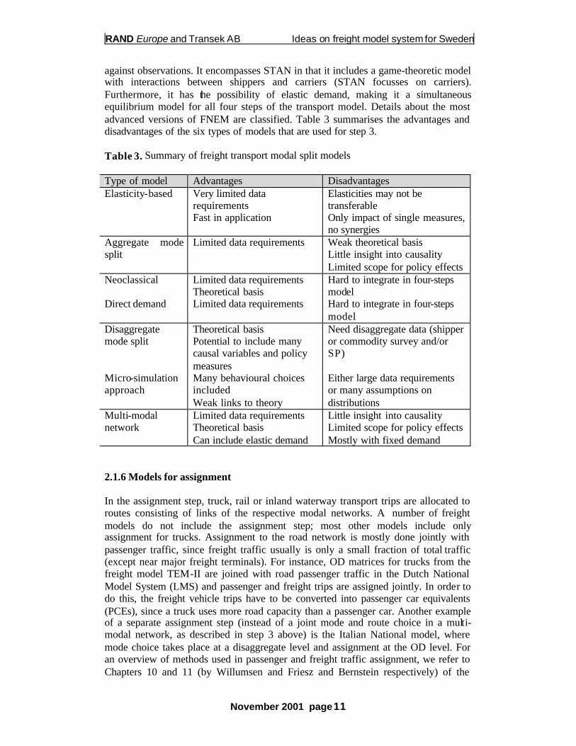
against observations. It encompasses STAN in that it includes a game-theoretic model with interactions between shippers and carriers (STAN focusses on carriers). Furthermore, it has the possibility of elastic demand, making it a simultaneous equilibrium model for all four steps of the transport model. Details about the most advanced versions of FNEM are classified. Table 3 summarises the advantages and disadvantages of the six types of models that are used for step 3. Table 3. Summary of freight transport modal split models Type of model Advantages Disadvantages Elasticity-based Very limited data

requirements Fast in application

Elasticities may not be transferable Only impact of single measures, no synergies

Aggregate mode split

Limited data requirements Weak theoretical basis Little insight into causality Limited scope for policy effects

Neoclassical Limited data requirements Theoretical basis

Hard to integrate in four-steps model

Direct demand Limited data requirements Hard to integrate in four-steps model

Disaggregate mode split

Theoretical basis Potential to include many causal variables and policy measures

Need disaggregate data (shipper or commodity survey and/or SP)

Micro-simulation approach

Many behavioural choices included Weak links to theory

Either large data requirements or many assumptions on distributions

Multi-modal network

Limited data requirements Theoretical basis Can include elastic demand

Little insight into causality Limited scope for policy effects Mostly with fixed demand

2.1.6 Models for assignment In the assignment step, truck, rail or inland waterway transport trips are allocated to routes consisting of links of the respective modal networks. A number of freight models do not include the assignment step; most other models include only assignment for trucks. Assignment to the road network is mostly done jointly with passenger traffic, since freight traffic usually is only a small fraction of total traffic (except near major freight terminals). For instance, OD matrices for trucks from the freight model TEM-II are joined with road passenger traffic in the Dutch National Model System (LMS) and passenger and freight trips are assigned jointly. In order to do this, the freight vehicle trips have to be converted into passenger car equivalents (PCEs), since a truck uses more road capacity than a passenger car. Another example of a separate assignment step (instead of a joint mode and route choice in a multi-modal network, as described in step 3 above) is the Italian National model, where mode choice takes place at a disaggregate level and assignment at the OD level. For an overview of methods used in passenger and freight traffic assignment, we refer to Chapters 10 and 11 (by Willumsen and Friesz and Bernstein respectively) of the



handbook edited by Hensher and Button (2000). They identify many approaches to the assignment stage: all or nothing assignment, stochastic assignment, multi-user class assignment, congested assignment, dynamic assignment. Table 4 summarises the advantages and disadvantages of having a separate assignment stage compared to combining the last two steps. Table 4. Summary of assignment models in freight transport model systems Type of model Advantages Disadvantages Separate assignment stage

Mode choice model can be disaggregate

Absence of interaction between demand and assignment can be unrealistic; this can only be done iteratively Transport chains are difficult, but not impossible, to incorporate

Multi-modal network

Substitution takes place between mode-route combinations Chains with different modes on a route can be handled

Little scope for controlling the optimisation process

2.1.7 Forecasting models in a broader context The review so far has concentrated on freight transport forecasting models. In many countries and regions, these forecasting models, are part of a larger system for simulating policy measures and estimating the impact of policy options through the freight transport system on a variety of performance measures (including emissions, safety, congestion, economic impacts, and noise). Indeed, in most cases this has been the objective for the development of the freight transport forecasting model. An example of this is the PACE-FORWARD model (see Carrillo, 1996) for Dutch freight transport, which enabled the assessment of policy options for several economic scenarios extending to the year 2015. Nearly 200 tactics that might be combined into various strategies for improving freight transport were identified and evaluated. Recommendations were drawn from a ranking of tactics based on their cost-effectiveness. 2.2 Existing data 2.2.1 National transport Within the Swedish borders in 2000, 390 million tonnes of freight were transported (domestic transport). 61 % was carried by lorries (with a loading capacity of 3.5 tonnes or more), 29 % was maritime transports and 10 % railroad. If the distance is less than 100 km, the majority is transported by lorry and if the distance is more than 300 km the majority is by maritime transports. The transport performance with foreign lorries in Sweden is not included in these figures.



The transport performance in ton-kilometres were 82 282 millions in 2000. 38 % was carried out by lorries (with a loading capacity of 3.5 tonnes or more), 38 % was maritime transports and 24 % railroad. 2.2.2 SAMGODS and transport statistics The SAMGODS model is based on Swedish official statistics, but in order to get useful matrices some smaller adjustments have been made. For the cost functions in the STAN-model there was the ambition to base these on official information, but in the present model the cost functions are based on a large number of different data sources. The calibration and validation of the STAN results in the SAMGODS model is mostly based on The Road and Railway Administrations’ vehicle counts. As the STAN results are measured in tonnes and the vehicle counts are in numbers of vehicles, there is of course a problem in finding the truth. The sum of transport performance in ton-kilometres in STAN has also been compared with Statistics Sweden’s official numbers. The border traffic in STAN has been compared with the official border traffic (road and ports). The main outcome of these comparisons was that for the base year 1997, STAN99 performed satisfactorily for railway transport, but not for road transport and especially not for maritime transports. The main problems are related to route choice for the Swedish surface part of the maritime transports: getting the flows of lorries (to a lesser degree trains) to and from the right ports in Sweden. 2.2.3 Transport statistics Lorries and trailers There is an annual survey, carried out according to EU-directives 78/546/EEC, called UVAV. The statistics are based on a stratified sample of about 8,000 Swedish lorries per year (total population 56,000) with a loading capacity of 3.5 tons or more. Each selected lorry is studied for one week and information is collected about the lorry itself and the transports (commodities, travel distance, weight, dangerous goods). The results are only statistically valid for transport between the 24 counties (and the three large city areas), but information about origin municipality and destination municipality is included in the survey. The UVAV survey (for several years) has been used to get the matrices for domestic lorries in the SAMGODS model. The matrices used in the SAMGODS model are for flows between municipalities’ (288). For this reason the SAMGODS group have used some additional statistics and done mathematical calibrations. Some of the UVAV information has also been used to gain more knowledge about the foreign trade, using a code which is stored for each origin and destination (the categories are: railway station, airport, harbour, lorry terminal and other place, such as factory, workshop, stock-in-trade and retailing).



The lorry statistics have been revised in 2000, according to EU rules (notably through EUROSTAT). The statistics now also include exports and imports done by Swedish lorries. The idea of EUROSTAT is that a system of Pan-European lorry statistics wil be developed. Surveys of goods transported by vehicles with loading capacity less than 2 tons have been conducted in 1991 and 2000. These transports are excluded in the current SAMGODS model. Yet in Sweden, the number of road vehicles with a loading capacity of less than 3.5 tons greatly exceeds the number of vehicles with a loading capacity above 3.5 tons, and the number of vehicle kilometres of the former category exceeds those of the latter. 90% of the vehicle kilometres by vehicles with a loading capacity under 3.5 tons is done by vehicles owned by companies. In the NAETRA model for the county of Stockholm these smaller vehicles are included. The NAETRA database uses a stratified sample of the 175,000 workplaces in Stockholm county for 1998. For each workplace selected, information on all movements during one day by a selected vehicle (heavy lorry, light lorry, car) was collected. The split of road traffic in the Stockholm county in terms of vehicle kilometres in this model is as follows: • Private cars for private use: 75% • Private cars (and small vans) in work-traffic: 8% • Business trips in cars: 5% • Lorries >3.5 ton in the county: 4% • Lorries > 3.5 ton with origin or destination outside the county: 3% • Lorries < 3.5 ton: 5%. Non-freight trips with (mostly privately owned) vans are included in SAMPERS, but freight transport with vans and small lorries are not in SAMPERS or SAMGODS. Given their share in total (goods) traffic, it seems very important to include the vehicles with lower loading capacity in the new Swedish freight model. The SAMGODS-model contains for domestic road transport only information on Swedish lorries. For non-domestic transport (import, export, transit), the distinction between Swedish lorries and transports done by foreign lorries on the Swedish territory can not be made in the present SAMGODS-model. Information about foreign lorries and trailers in Sweden has been surveyed in 1987 and 1990. In 1990, foreign lorries in Sweden accounted for 290 mln vehicle kilometres and 3,150 mln ton-kilometres. In the same year Swedish lorries made 26,519 mln ton-kilometres in Sweden. Therefore the share of foreign lorries was about 12%. This is a sizeable amount, which should distinguished within the model system, especially when it comes to assignment to the road network. In 1988 and 1991 the Swedish international road transports were surveyed and since 1995 international road transports are reported according to EU-directives. Railway transports Each railway company has to deliver statistics about total freight (tonnes and ton-km) per commodity group each year. The railway matrixes used in the SAMGODS model



come from the Railway Administration and consist of the official statistics and some not-official information from the railway companies. Maritime transports In the official statistics there is information from each port about loaded and unloaded goods. The information is divided into loaded/unloaded from domestic ports and loaded/unloaded from foreign ports (tonnes and NST/R coded commodities). Short sea shipping is included. Air transports In the official statistics there is information about each airport regarding the total number of tonnes loaded/unloaded. There is no information about type of goods, destination airports or about the actual origin and destination of the transport chains (including transport to and from the airports). SIKA has commissioned a small survey to gain more knowledge about type of goods in air transports. In the survey large companies have been interviewed about their air transports and customs statistics have been analysed. In the survey about a third of the freight by air has been mapped out. The report will be delivered to SIKA in October 2001. Air transports are not included in the current model, but as the freight traffic by air is constantly and relatively rapidly growing, including air transport in the new SAMGODS model would constitute an important improvement. The commodity flow survey This survey is ongoing during 2001 and is a part of the official Swedish statistics. SIKA, the Traffic Administrations and the Board of Communication finance the survey. Statistics Sweden is carrying out the survey. The purpose of the survey is to give a picture of the commodity flows in Sweden and between Sweden and other countries (goods volumes, commodity values, and means of transport). The statistics are based on a stratified sample of compa nies (place of work) within different sectors (mining and mineral industry, manufacturing industry and wholesale trade). Investigative work has been done to examine whether it is possible to include agribusiness and forest industry in the commodity flow survey, with a positive outcome: these are included now. Each company’s transports are measured during one week. In summer 2001, there were indications that there could be problems with inconsistencies in the data, but these appear to have been solved now. The survey defined the end destination of the goods, but the data from companies could be based on their main office or branch actually delivering the goods. The commodities should be coded in NST/R codes.



2.2.4 Economic statistics Foreign trade - international transports As a large part of the Swedish production is exported and the Swedish consumers and industry have a demand for foreign goods, it is important to include international trade in order to get a full picture of Swedish transport. Since 1995 the official trade statistics are the same as in all other EU countries. National Accounts The Swedish National Accounts (NA) sum up and describe the national economic activities and development as a system of accounts in a consistent and coherent way. The accounts comprise the production and consumption of goods and services, allocation, reallocation, the uses of income and capital formation and transactions with the rest of the world. In connection with the calculation of production values, figures on employment in terms of number of employed and hours worked are also compiled. The quarterly NA showing recent economic developments are released mainly with information on production and consumption. The annual NA is more detailed and includes accounts for income and savings in the institutional sectors. Revised values in quarterly accounts for earlier years may be more frequently updated than those for the same period in the annual accounts. Annual accounts are revised once a year. Since 1999, the NA have been adapted to The European System of National Accounts (ESA 95), which is fully consistent with the worldwide guidelines for national accounting (SNA 93). Figures in constant prices are calculated in the prices of the immediately preceding year. The series are then chained to the reference year 1995. To meet the needs for longer time series, backward calculations have been carried out in accordance with ESA 95, using previously calculated series. Industry statistics All companies (with more than 10 employees) in the manufacturing industry have to fill in a form about where they are located, how much they manufacture, type of products and volume. This information is used to compile the industry statistics. Input-output tables The official input-output (I/O) tables were from 1985. New tables (year 1998) have been determined recently. The ones from 1985 have 31 sectors; the 1998 tables have 38 sectors. These I/O tables are at the national level. In a project called RAPS, regional I/O tables have been produced, based on both observed and synthetic data. It is not clear to us whether these regional I/O tables would be available for the development of a new SAMGODS model or what the quality of this data is.



2.3 The present SAMGODS models and tools 2.3.1 Introduction The SAMGODS model is documented in English in the report “The Swedish model system for goods transport SAMGODS” SAMPLAN Rapport 2001:1. In this section an overview of SAMGODS is given and some problems and disadvantages in the different modules of the SAMGODS models are pointed out. These are problems and disadvantages not yet mentioned in the list in Section 1.2, making the total list of weaknesses even longer. The SAMGODS model consists of six modules (seven if one includes the totally separated modules for CBA). Five of them are used to generate the demand for freight transports and the sixth is a network model. The modules are run separately and much effort has been made to get the output from one module to “fit” into the one that follows. 2.3.2 ISMOD SIND (“Board of Industry”) originally developed the ISMOD model in the early/mid 1980s. ISMOD has since then been used for long term economic forecasting for the Department of Finance. During the last ten years the model has only been used by NUTEK (the Swedish National Board for Industrial and Technical Development) and SIKA. In recent years, at the School of Economics in Jönköping, the model has been adjusted and re-estimated with new data. This “new” model has got the name “ISMOD 2000”. It would be possible to use this updated version in a new model system for Sweden. The ISMOD model is formulated to generate solutions valid for the time period of 5-15 years ahead. The time period should not be shorter due to investment processes and not longer because the input data (technology alternative) becomes less adequate when the time period is longer. The model can be described by the following the parts.

1. Production structure: The basis is input-output matrices, in which each sector’s demand for input delivery is determined and input coefficients are specific for each technical category in the sector. There is a limited capacity in the model. The capacity can be extended during the time period, but it requires investments and that investment generates a demand for deliveries from other sectors (according to a vector of investment coefficients). At the same time there is a reduction of capacity in some of the sectors. The profit level in the sector determines the speed of the reduction (in turn determined by prices and wage level).

2. Supply of goods and services: During the time period, the supply is changing

due to (i) capacity reduction, (ii) investments in new capacity and (iii) imports. All three components are dependent on the equilibrium prices during the time period.



3. Demand for goods and services: The demand side has the following five

components (i) current purchase for the production, (ii) private consumption, (iii) purchase for the public sector, (iv) export, (v) purchase of investment goods. The demand components are directly and indirectly dependent on the equilibrium prices.

The production capacity for each sector is given for the base year. Given this starting-point, the model solves a condition in the economy for the last year in the time period. The economic condition is described foremost by a sectoral balance of resources.

One problem with ISMOD (and Early) is that they operate with industry sectors and not commodity groups. A translation exists between sectors and the commodity groups used in the SAMGODS model, which has been used by SIKA and others. In ISMOD, trade and transport are treated in a very simplistic way. The output of these sectors is assumed to amount to the aggregate trade margins of the other sectors. Experience shows that changes in transport costs and infrastructure investment have an impact on the sectoral structure and transported volumes and quantities. In ISMOD this is not possible. It has been planned to develop a version of ISMOD (ISMOD-T) with better representation of transports. There is no geography in ISMOD. Another problem is, of course, the time horizon. Analysing infrastructure investments require long forecast periods. For both the SAMPERS and the SAMGODS models, special regional forecasts of population and employment have been conducted by different consultants (based on international forecasts). 2.3.3 Early Early is about 5-10 years old and has been developed by NUTEK (the Swedish National Board for Industrial and Technical Development) for regional analyses of employment in Sweden. The model uses the results from ISMOD to generate regional forecasts of employment per sector. The regional employment by sector for a base year and a forecast year is used as input to SAMGODS, to distribute the national production for the forecast year. The regional change in employment between base and forecast year serves in SAMGODS as an indication of the regional change in production. There are at present no satisfactory links between SAMPERS, STAN and Early or regional demography and migration on one side and regional consumption, employment and production on the other. 2.3.4 Model for calculation of implicit price/ton for commodity aggregates The economic model determines the future demand and supply in the economy measured in economic values; the transport flows are defined in quantity terms. To be able to generate future O/D-matrices in tonnes there is a need for implicit prices that



can convert values into quantity. This implicit price for each commodity group has been calculated by using trade statistics (this was last done in 1998 by a consultant). Regression analyses (time series) and different assumptions have generated the price/ton-values, which are used in the present SAMGODS model. Some disadvantages of the current implicit prices are: • In the trade statistics not all commodities are measured in tonnes (this is probably

a minor share). • The trade statistics uses the CN nomenclature and the transport statistics the

NST/R codes; there is a conversion table but it is not fully sufficient. • The mixture of commodities in a commodity group is varying over time and it is

difficult to make forecasts for the mix of commodities (and to include new commodities).

• The trade statistics should only be used for the implicit prices for export and import, but no other data material is available.

• The implicit prices differ for production, import and export but have no regional differences. In reality the implicit price vary because the mix of commodities varies between different regions. However this is not regarded as a major problem by SIKA: the idea is that in practice these differences are only small.

2.3.5 Model for interregional domestic transport demand This model is from the early 1980s and was developed for TPR (the Board of Transport) for freight analyses. The model has been further developed during the last ten years and, for example, the output from the model now consists of matrices that can be used directly in STAN. This model uses the output from ISMOD, Early and the implicit price/ton to generate domestic O/D matrices for commodity groups measured in tonnes. This is being done using an entropy algorithm to estimate forecast demand matrices for relevant commodity groups. Estimates of the present domestic interregional transport flow matrices based on available data as well as corresponding foreign trade matrices are used as a priori matrices in the entropy algorithm. The marginal conditions for each commodity is delivered from the ISMOD-model output. The model is very conservative, since the pattern from the base year is guiding. For exports, import and consumption/investment the proportions per region are assumed to remain unchanged between the base year and the forecast year. And the actual proportions are from the early 1980s. 2.3.6 Model for subcountry level region-to-region Swedish foreign trade The latest model is the model for subcountry level region-to-region Swedish foreign trade. Two consulta nt companies (Inregia and COWI) in co-operation developed this model in 1999/2000. The model is not yet fully integrated with the other modules in the SAMGODS model group, but has the large advantage to have a user-friendly interface, which allows the user to either use default values or make his own assumptions.



As the domestic transport demand model, the subcountry level for Swedish foreign trade uses input data from the ISMOD model (in this case: exports and imports by sector at the national level). The model has two main modules. The first one is a bilateral trade forecast model and generates trade forecasts for the total Swedish foreign trade per trade partner. The second part determines the distribution of the total trade to bilateral trade flows. From the second part of the model the user gets sub-regional to sub-regional O/D matrices for Swedish foreign trade. The O/D matrices can then be used as input directly in the STAN model to get transport flows per mode of transport and links. 2.3.7 STAN The STAN model has been used in Sweden since 1990 for network analyses. In 1994/1995 the STAN package (STAN95) began to be used in for investment planning by the road and rail administrations. A thorough revision of the 1997 STAN-implementation was carrie d out during 1998 and 2000, and work on improving STAN is still going on. The revision included implementation corrections and improvements as well as an overhaul of the cost functions. The SAMGODS group changed the STAN software version at the same time (better, faster, and more capacity). The assignment relates only to the transport flows between the zones. The transit traffic through Sweden is represented in two matrices, one for lorries and one for rail. These O-D matrices can be distributed to the ne twork links together with other intrazonal traffic. At the level of the total country, lorry transport is 12% of total road traffic. In the link cost function the total flow on a link is first divided by 0.12 to get the total flow on the link. Then the volume-delay function is applied. This implies that STAN assumes that the proportion of lorries on every link is 12%. This is evidently not a good assumption; this share will vary considerably. Moreover, some of the vehicles under 3.5 tons are not included in the assignment. In the STAN99 model there are: • 13 vehicle types • 6 products • 14 volume-delay functions for road links • 3 volume-delay functions for railway links • 4 types of connector links (‘skafts’) between a zone centroid and the network • 42 different reloading costs (between vehicles) In the STAN implementation the SAMGODS group uses, the costs on links and in nodes are divided into operating cost (OC) and quality-related cost (QC): OC on a link = distant dependent cost (= kilometres times value per km)

+ additional cost for some railways (km +2%) + time dependent cost (hours times value of time) + special cost on links (cost per link) + starting cost at the ‘skaft’ (cost per link).

OC in a transfer node = the reloading cost (cost per reloading)



QC on a link = risk of delay (kilometres times risk per km times value of the risk) + value of time (hours times value of time) + a frequency related cost on the ‘skaft’ (hours times value of time). QC in a transfer node = risk of delay (risk per reloading * number of reloadings

* value of risk) + value of time (reloading time * value of time)

+ a frequency-related cost when reloading (waiting time * value of time)

The cost functions outside of Sweden are modified to some extent: • For railway there are additional cost for transport outside Sweden (+40% for most

countries outside Sweden, since in Sweden the rail fares are relatively low) and the volume-delay functions are not used outside Sweden (transport time is not affected by congestion), but replaced by speed (there is some information about time lost at major bottlenecks).

• When passing a border, there is a special delay risk cost and time cost. The STAN program has itself advantages and disadvantages. The STAN system solves the problem by using a system optimum solution. It has been discussed whether freight transport should be analysed from this point of view. If one only studies a monopolistic railway company, there is no problem but if there are a number of different decision-makers, the STAN approach might be problematic. On the other hand, calculations have shown that if there is “free flow” in the system the difference between a user and a system optimum is quite small. In the implementation both mode and route choice is carried out in the STAN system. This can of course be right for some transports but is totally wrong for others. The present version of the system doesn’t include intrazonal transports. However, 17% of the tons transported by road in Sweden is for distance below nine kilom etres. This accounts for 26% of the shipments in goods transport by road. On the other hand these transports only constitute 1% of the ton-kilometres. The zoning system in SAMGODS (288 zones in Sweden) is rather fine, compared to many other freight models. Collecting and publishing information for even smaller zones might raise problems of confidentiality, because flows related to individual firms might then be identified. 2.3.8 The evaluation module Estimates for carrying out socio -economic evaluations of communication sector projects, including both passenger and freight transport, have been revised recently (Summary of ASEK estimates, SIKA report 2000:3). This report includes the prescription to use a discount rate of 4%, 1999 prices and discounting to 1-1-2002, recommended lifetimes for different types of infrastructure, tax factors and values and formulae to convert the following impacts into monetary terms: • Accidents • Air pollution (regional and local effects)



• CO2 emissions • Noise • Time (in passenger and freight transport) • Cost (in passenger and freight transport). At the moment, a number of effects cannot be included in the monetary evaluation (e.g. natural and cultural values, encroachment, employment and economic growth). The recommendation in the SIKA report is to include descriptions of the consequences on such items in the project plans. The ASEK estimates have been adopted for the ongoing planing review for the period 2002-2011. This procedure is especially used by the road and rail administration. For maritime and air projects, the situation is different, since the ports and airports are often owned by the municipality or jointly by the state and the municipality. The outputs of STAN consist of tonne-kilometres and generalised cost. For input into cost-benefit analysis more detailed information is required. At the moment SIKA is carrying out a project to produce extra outputs from STAN: also vehicle kilometres, transport cost, transport time. This information can be used almost directly in cost-benefit analysis. Later on, other work about distinguishing vehicle types, which is an important input for calculating emissions, noise and road damage, might be carried out.



3. Proposed New Model System for Freight Transport 3.1 Basic ideas behind the suggested approach

We have in mind building an integrated family of mutually consistent models of the same phenomena at two different levels of resolution: (1) a detailed (high-resolution) set of models, and (2) a fast (low-resolution) policy analysis model. There are several reasons for building such a family of models. These include: • Information needs : There will be many types of users for the models, who will

be trying to answer different types of questions and to obtain different types of information. One cannot readily use models from one level to understand and accommodate information needed at a different level. This suggests the need for models (not just data displays) at different levels of resolution and with different perspectives on the freight transport system.

• Cognitive needs : The output from a detailed model is often designed to be used and interpreted by analysts, not decision advisors. And, even if the model will be used by analysts, humans reason at different levels of detail and therefore require information at different levels of detail. The model does not do the analysis; it provides inputs for the analysis, and the input should be “user friendly”.

• Economy: It is sometimes necessary to use a low -resolution model, because high- resolution comes with a cost. High-resolution models require more input data, making cases harder to describe, longer to prepare to run, and longer to run. For some purposes (e.g., for policy analysis), a faster, low-resolution model is preferable (see the next subsection).

• Accuracy: Sometimes the extra time and effort to prepare and run a case is needed, because an accurate estimate is required, and sometimes this extra time is not needed. When decisions have costly consequences, decisionmakers are likely to value predictions free of bias and forecasts with low mean square error. Moreover, the decisionmakers will often want detailed information in such situations. On the other hand, if one is looking for big differences among estimates (e.g., big differences in policy effects), the simplifications only matter if they would affect the conclusions (e.g., choice of policy).

When building a model for a single user, as in many traditional decision support systems, the trade -offs among speed, detail, and accuracy can usually be made within a single model. In this case, the user’s needs can be defined narrowly enough that a single model can be tailored to meet all of them. However, in the case of a national freight model system for Sweden, we do not suggest that a single model be built to serve the needs of all of its potential users in terms of speed, detail, and accuracy. Instead, we suggest building a family of several models, each one satisfying different needs and each one satisfying the principle of Occam’s razor: it is the simplest model for the desired purpose, but not simpler.



3.2 The proposed model structure Figure 1 below gives an overview of the proposed model structure. The numbers over the boxes refer to the subsections below in which the specific model is discussed.

Disaggregate mode (and shipmentsize) choice model on SP/RP data atnational/international level

Assignment

Detailed Forecasting Model Fast Policy Analysis Model

System dynamics model with:• macro-economic module• land use module• transport module • environmental module

3.2.1

3.2.2

3.2.2

3.2.2 3.2.2

3.2.3

Logsum

Transport cost and time

Transport cost and time

I/O model (+ regionalisation module)for production/attraction and distributionmodel at national/international level

Evaluation modules

Disaggregate model linked with passengermodel at regional/urban level

Figure 1 – Overview of model structure The various components of the model are described below. 3.2.1 A Fast (Policy Analysis) Model One of the many uses of the family of models will be for policy analysis. Policy analysis is a process that generates information on the consequences that would follow the adoption of various policies. It uses a variety of tools to develop this information and to present it to the parties involved in the process in a manner that helps them come to a decision. Its purpose is to assist policymakers in choosing a course of action from among complex alternatives under uncertain conditions. The word “complex” means that the policy being examined deals with a system that includes people, social structures, portions of nature, equipment, and organisations; and that the system being studied contains so many variables, feedback loops, and interactions that it is difficult to project the consequences of a policy change. Also, the alternatives are often numerous, involving mixtures of different technologies and management policies, and producing multiple consequences that are difficult to anticipate, let alone predict. In a policy situation as complex as that dealing with freight transport in Sweden, it is easy to become overwhelmed by the “curse of dimensionality.” That is, there are so



many possible alternatives, so many uncertainties, and so many consequences of interest, that it would be difficult to evaluate the complete range of consequences for each alternative and a wide range of scenarios. One way to deal both efficiently and effectively with this situation is to use a fast model to gain insights into the performance of the alternatives. A more detailed model in the family might then be used to obtain more information about the performance of the most promising alternatives. Assessments based on the fast model, therefore, would be considered as first order approximations in discussions on transport or related policies. When a promising policy has been identified using the fast model, it will often be necessary to conduct further detailed planning and research in which full account can be taken of the specific circumstances and characteristics of the problem. Design Considerations A policy analysis model must be designed around the information needs of its users. Thus, the first step in designing the fast model will be to assess these needs. There is no requirement that the fast model need be an aggregate version of the detailed model(s) in the family. In fact, because it is fast, it can contain features that would be impossible to include in the high-resolution models. High-resolution models must be limited in scope, lest they become so unwieldy as to be useless. Also, they are intended to be used for different purposes, so their outputs will be different. For, example, we expect that the fast model will have impact assessment modules for estimating not only the effects of changes in policies and/or changes in scenarios on transport demand (which will be the focus of the high-resolution models), but their effects on the national economy, regional economies, land use, and the environment. Figure 2 shows how the planned uses of a model are major considerations in determining the model’s scope (number of factors included in the model) and its depth of detail (amount of detail for the factors that are included). Policy analysis models are intended to be used primarily for screening large numbers of alternative policy options, comparing the impacts of the alternatives, and designing strategies (combinations of policy options). They should include a wide range of factors (e.g., a variety of impacts, geographical regions, commodities), but little detail about each of the factors. The outputs are intended primarily for comparative analysis (i.e., relative rankings), so approximate results are sufficient. Implementation planning, engineering, and scientific models are needed for examining fewer alternatives according to a smaller number of factors. But they are used in situations where absolute values are needed, which requires more accurate estimation of the results for each factor. Although different in scope and outputs, all models in a family must share certain characteristics. A key design consideration is how to reconcile the system concepts and outcome estimates among the resolution levels. It is often assumed that the correct way to do this is to calibrate upward: treating the information of the most detailed model as correct and using it to calibrate the higher-level models. This is often appropriate, but, as mentioned above, the more detailed models will have different scopes and outputs. Further, different models of a family may draw upon different sources of information. Davis and Bigelow (1998) make the point that members of a multiresolution model family should be mutually calibrated. In some cases, aggregate information may be used to calibrate more detailed models, while



most calibration is likely to be in the other direction. However, it is important to acknowledge that there are limits to how well lower-resolution models can be (and need to be) consistent with high-resolution models. Approximation will be a central concept from the outset. Consistency between two models should be assessed in the context of use. What matters is not whether two models generate the same numbers, but whether their implications are the same (e.g., they would lead to the same rank ordering of policy alternatives). Differences in the assumptions underlying the models must be made clear, as well as the contexts within which the models should and should not be used.

Breadth of Scope (number of factors)

Dep

th o

f Det

ail (

per

fact

or) Policy analysis models

(screening, comparisonof alternatives)

Implementation planning,engineering, scientific models

Impractical (but frequently attempted, usually with disastrous consequences)

Figure 2 – Different types of models have different scopes and levels of detail In addition to being fast, so that a large number of policy options can be examined in a short amount of time, the low-resolution model should provide easy, user-friendly ways to reflect changes in the system due to changes in policies or scenarios (i.e., to change the model’s inputs). Its impact assessment modules should also include ways of reflecting a range of such changes in the estimation of impacts (in order to produce the relevant outputs). The latter requires some understanding of the policy options that might be considered. For example, if the emission estimation module refle cts only road vehicle emissions, it will not capture the true emissions changes due to modal shifts; and if it does not reflect the nature of the fleet of freight vehicles, it will not capture the effects of a changing mix of trucks. For the fast model, I/O output analysis or sample enumeration with discrete choice models is not a feasible option, due to the run times and data requirements involved. For this model our advice is to rely mostly on system dynamics models. Dynamic models, such as system dynamics models, have the additional advantage of not only incorporating interactions and feedbacks among transport, land use and the economy within a single forecast year (or for a few intermediate steps), but providing a time path. They simulate the time path of the development of a system and its behaviour. Dynamic models are especially useful for modelling the long-term performance of a complex system (like the freight transport system) whose determinants change with



different speed or intensity over time, and which is connected with other complex systems (like land use and the economy), whose components also change over time. Dynamic models are also particularly appropriate for assessing the performance of policies that are defined as functions of time (i.e., policies that change over time or whose pieces get implemented at different points in time). The ASTRA System Dynamics model platform (ASP), which was developed to perform integrated long-term assessment of European transport policies, is a good illustration of this approach. It simulates the dynamic interactions and feedbacks among four sectors using four submodels: (1) macroeconomic model, (2) regional economic and land use model, (3) environmental model, and (4) transport model. Dynamic models could also be used to provide forecasts on population, employment, GDP, etc., which are inputs to the freight transport model. In most cases, the fast model system will include mechanisms for transforming the system changes produced by the various policy measures into model variables, e.g., through the use of elasticity relationships. This is an approach that RAND Europe used successfully in the TRACE project, which it carried out for the European Commission. For example, the price elasticity of demand, within a carefully defined segment of the market, can be used to translate an increase in fuel price into a change in transport demand. The imposition of distance-based road pricing can be translated into an equivalent change in the fuel price, and its effects estimated using the fuel price elasticities. At the moment, the EXPEDITE consortium is using similar methods to apply results from national passenger and freight transport models (including SAMPERS and SAMGODS) within a fast European-wide model for the European Commission - DGTREN. The elasticities for the low -resolution model can be based on accepted published results and/or from fitting functions to the output from experiments with high-resolution models. (In the latter case, the elasticity is called a “repr o model”, since its behavior “reproduces” the behavior of the more detailed model.) 3.2.2 A detailed model for international/national freight transport An input-output model for production/attraction and a distribution model According to the terms of reference, a model system is needed that includes feedbacks from transport to land use (e.g. regional economic development). In the literature there are basically two ways of doing this: integrated land use–transport models and system dynamics models. No system dynamics model has been developed that predicts outputs in the form of flows between a large number of origins and destinations and network loads and the sensitivity of these to policy changes, and we do not foresee the development of such models. These outputs however are required from the new Swedish freight model, although not for all applications. That is why we recommend to develop a fast model using system dynamics concepts on the one hand and another detailed model that will be capable of providing outputs in the form of OD matrices and network flows on the other hand. If this latter model must also include feedbacks to land use, the only feasible option (besides developing something entirely new for this) is to use integrated land use/transport models that rely to some extent on I/O tables.



Integrated land use–transport models typically include an input-output (I/O) submodel as a first step toward the OD demand matrix, transport markets and land markets, with equilibration mechanisms. We understand that Sweden until recently did not have regional I/O statistics, but only national data on this. The present I/O model (ISMOD) therefore is a national sectoral model. ISMOD is not a standard I/O model; a number of price mechanisms and time-series-based changes in productivity by sector have been included over the years, so that it now is somewhere between an I/O model and a computable general equlibrium (GCE) model. This model could be used as the basic I/O model, or an update on new data (1998 I/O statistics), to yield trade flows between sectors. To get trade flows between sectors located in different regions, a regionalisation module (based on entropy or gravity type or logit models) might be used, as happens in the Italian national model for freight transport (which contains disaggregate mode choice, but aggregate generation and distribution). In the RAPS project, regional input-output tables have been produced, partly based on observed data, partly synthetic. These can be used, if available and suf ficiently reliable, to get trade flows between regions without a regionalisation module (or with less dependence on a regionalisation module). In state-of-the-art transport models, such as the Italian national model and the SMILE model, input-output or related models are used. Also the prototype freight transport model for Portland and the proposed model structure for London contain input-output models (Neffendorf et al., 2001). In Sweden, recent (1998) I/O data are available; maybe even regional I/O data can be used. We recommend that an I/O model be part of the new detailed international/national freight transport model. A major disadvantage of using I/O models is that the I/O data and models are in money units (trade flows). A freight transport model should produce flows in terms of tonnes, tonne-kilometres and vehicle -kilometres. In transport model systems with I/O models a conversion usually takes place from money units to tonnes, using fixed weight to value ratios. These ratios are usually based on mean values from the trade statistics and mean weights from the transport statistics for commodity classifications that are assumed to be uniform. This is one of the weakest points of model systems using the I/O approach, or indeed any other economic model. To include economic development, world market prices, production, consumption and trade in a freight transport model, the only possible way seems to be to use an economic model (I/O, CGE) which uses money units. We recommend strengthening this weak link by carrying out specific surveys among shippers asking about the value and the weight for the same shipment and about its frequency. The commodity flow survey will also include questions about the value, weight and frequency of shipments and can be used to obtain a better value to tonne conversion as well. To make traffic generation (production and attraction) and distribution dependent on transport times and cost, the technical and trade coefficients in the I/O model need to be elastic (with time and cost, e.g. in a logsum variable from mode choice as explanatory variable), as in the Italian national model and the SCENES model. The transport disutilities can be used as feedbacks (with a time lag) to land use (location of population and employment). An I/O model based on Swedish I/O tables will not give international transports through Sweden (because these trades are not connected to inputs and outputs that are in the tables). This has also been mentioned as one of the weak points of the present



SAMGODS model. Furthermore Swedish I/O tables might be less appropriate for giving transports to and from Sweden. For transport through Sweden, outcomes from existing international projects might be used (e.g. from passenger and freight transport models developed for the European Commission, such as SCENES or EXPEDITE, or international corridor projects such as Fehmarn Belt and Öresund). An alternative would be to use not the model results, but the database, to develop new international models focussing on Sweden, as was done in developing SAMPERS For policy analysis of likely changes in the volume of through transport (e.g. impacts of Eurovignet), an international model, including the behaviour of Danish, German, Dutch, etc. shippers/carriers is needed. For getting trades between Swedish regions and foreign countries it might be worthwhile to keep using the model recently developed by COWI and Inregia in the future SAMGODS, instead of deriving these trade flows completely from a new I/O model. A disaggregate mode and shipment size model Disaggregate behavioural models are very uncommon in freight transport – unlike passenger transport – for two basic reasons: • absence of data on disaggregate units of observation; • difficulties encountered in the estimation when disaggregate data are available;

mode choice model estimation on shippers’ surveys in some cases has not been successful due mostly to correlation between time and cost components.

It might be possible to develop a mode (and shipment size) choice model on the new shipment survey combined with a proposed new SP survey. The SP survey then needs to be carried out to obtain time and cost information that unlike the RP is not (highly) correlated. Such a disaggregate submodel can then be used in application through sample enumeration, as has been done for several passenger transport models. The proper design (who to interview, which contexts used for presenting hypothetical alternatives, which kind of alternatives offered at the same time) is crucial for getting a good understanding of decision-making in freight transport. Modes to be considered are road transport (maybe with several vehicle types), conventional train, combined (road-rail) transport, short-sea shipping and ferry transport and air transport. Transport activities increasingly take place within a larger context of logistic choices (including inventory policy, warehouse location, consolidation of flows to distribution centres). Such considerations can be added to the freight transport model in a disaggregate fashion, as Ben-Akiva and co-authors did in the 1980s on RP data and in the 1990s on joint RP/SP data. This can also be handled in an aggregate way as has been done in the SMILE model (which includes the choice of location and use of distribution centres between the origin and destination of the shipment) and in the SCENES appended module. We recommend to treat the wider logisitic choice processes in the context of disaggregate modelling on joint SP/RP data. The databases for a simultaneous estimation can be the commodity flow survey plus a new SP/RP shippers and carriers survey. The increased awareness of the logistic context also has repercussions on the commodity classification. Ideally this should be based on the handling characteristics of the goods being transported and also on the related issue that different commodity groups may have different values of time. The categories that are created when using



attributes with regards to logistic processes are sometimes called ‘logistic families’. In some cases it has proved possible to translate a detailed classic commodity classification (NSTR) into logistic families. Assignment If a separate disaggregate mode choice model could be developed for freight transport, the task remaining in the assignme nt would be route choice only, not mode and route choice as in the present STAN module. It might still be possible to do route choice based on cost minimisation rules in STAN. Given that ‘modes’ in this case are, for the purpose of shipments, sequences of modes (modebundles) for all but road transport (the only mode that can realistically take goods from origin to destination without transhipment), an issue to be resolved is the extent to which the choice process is most realistically handled by a simultaneous modebundle-and-route choice (STAN), or a choice of modebundle followed by route choice. At this stage one also needs to account for empty return trips. 3.2.3 A detailed model for regional/urban freight transport Introduction All the above ideas on the detailed model relate to models for freight transport to/from Sweden and between ‘not too small’ regions in Sweden. For the detailed model at the regional/urban level we recommend using disaggregate behavioural models, not I/O models. We would prefer ut ility or profit maximising choice models for this instead of using the Monte Carlo micro-simulation approach. E-commerce (business to business and business to consumer) can be expected to continue growing rapidly in Sweden, which has a high degree of Internet penetration and a high labour participation rate. Ordering goods through the Internet will have a large impact on future goods flows, both in terms of shipment size (mostly becoming smaller) and types of vehicles used (small lorries and vans). An increase in lorry and van trips will increase road congestion. Policies such as road-pricing (in selected urban areas) might be able to counteract these developments. This would be another proper area for carrying out SP surveys. We suggest to combine these with the SP/RP surveys mentioned above (e.g., one of the SP experiments could include road pricing). Models of freight movement are commonly acknowledged to be at a much lower state of sophistication than their equivalent in the passenger movement sector. There are many reasons for this, primarily associated with the enormous diversity of the freight market. An obvious first step in the reduction of this diversity is to sub-divide freight, and this is the usual first step for most models. For longer-distance movements, commodity type is the natural first categorisation to make, and then shipment size . ‘Values-of-time’ emerge as useful constructs in deciding on choice of mode, as they do for passenger movements. Splitting processes into Production (or Im port), Intermediate Processing, Storage and Consumption (or Export) then offers two options. Models equivalent to the Gravity Model for passengers can be assembled when Intermediate Processing is of lesser importance



(e.g. fresh eggs or coal), and Spatial Input-Output models can be developed where Intermediate Processing is crucial (e.g. pastries, steel). Storage (warehousing, collected depots) can be introduced into a cost -minimisation problem with minor difficulty, simply by offering alternative ‘hyper-routes’ between origin and destination (Production and Consumption) that use such facilities and that have different cost, delivery time, quality etc. characteristics. The focus of this section (Section 3.2.3) is on the very last part of the chain, leading to Final Consumption. Here, we are thinking of the physical movements, made by actors or agents in the supply of goods, that immediately precede the consumption or use of the goods. These include

• Delivery of goods to shops • Delivery of materials to offices • Delivery of goods and services to homes.

These can happen on a frequent, middling-rare or rare basis: for shops (and showrooms), we might have

• Frequent: newspapers, fresh food and drink • Quite frequent: processed food and drink • Middling rare: books, stationery, medicines • Rare: clothes, white-goods, computers, cars

For offices we would have a similar list, with some important differences

• Frequent: mail and periodicals • Quite frequent: parcels, computer paper, processed food and drink • Middling rare: computer equipment, stationery • Rare: furniture, carpeting.

For homes, we might have

• Frequent: mail (and in some countries, milk) • Quite frequent: parcels • Middling rare: light services (plumbers, electricians, salesmen) • Rare: furniture, carpeting, heavy services (painters, builders)

Some of these (e.g. light services) are not usually included in freight transport, but these should be accounted for somewhere in a national model system, because all types of road vehicles matter when it comes to assignment to the road network. All of these ‘destinations’ generate movements of ‘freight’ for taking things away, too; however, waste disposal activities are not pursued further in this section. Note that ‘mail’ nowadays includes messenger -service parcel deliveries on an increasing scale in business areas. Other sectors that we should note for the future include the police, fire and ambulance services, which are ‘service providers’ for all of home, shop and office destinations at some time.



In terms of ‘users of road-space’, we might even consider maintenance crews, repairing pavements, maintaining street-furniture and so on. These users might be considered to be a fourth generic ‘destination’ – the road space itself. The purpose of this section is to consider the pr oblem of understanding and forecasting the load on networks (mainly, but not confined to urban networks) which comes from the last non-final-consumer movement into final consumption. Thus, although we know there is a shopping trip needed to ‘bring the bacon home’ (for example), we are assuming this is already reasonably modelled as a personal trip. The ‘angle’ or perspective we are going to take is one in which we approach this problem after having constructed a disaggregate demand model for personal travel, such as SAMPERS, with all that implies for data bases. This section is intended to be the point of departure for recommendations on the type of data needed and sort of models to be developed, to allow proper insight into the forces and constraints leading to the movement of freight vehicles around networks for these ‘final-non-consumer’ trips. The Scale of the Problem Accurate figures of freight movements are not immediately available at the time of this writing. However, broad order-of-magnitude figures for the relative importance of freight vehicles to planners are as follows. (Note ‘pcu’ is used to denote passenger-car-units, so that a 1 pcu vehicle causes as much traffic interference as 1 car, a 2.4 pcu vehicle around 2.4 times as much (in terms of road capacity used up), etc.). Table 5. Freight vehicles as a component of all road traffic (in vehicle km and passenger-car-unit km ) % all km % all pcu % urban km % urban pcu all road freight 10 ~20 5 ~10 Light goods vehicles (LGVs) 1 ~1.5 10 ~15 (Hypothetical figures, to be validated and improved) The broad picture is that LGV activity, whilst minor in the ‘big picture’ of numbers of vehicles, is an important contributor to urban traffic congestion. As we have said, in our opinion it is also usually rather poorly measured and modelled in the base year, and future year forecasts are usually even worse. The purpose of the current section is to address one part of a possible solution, based on the use of information from personal disaggregate travel demand models to improve base year information and improve forecasts, including linking factors affecting demand for personal travel to factors affecting freight movements. In addition, this approach would offer a chance to improve the network supply/demand processes that should jointly affect both freight and passenger transport.



Input and output features of passenger demand models that should affect predictions of LGV activity. We are assuming that the necessary background data (behavioural diaries, contextual networks and zonal data, validation data) are available, as indeed is the case in Sweden. A modern disaggregate model like SAMPERS contains income information at the zonal level and a prototypical sample of household units. Network speeds in the base year will also be available, together with a base -matrix of passenger flows, preferably along with counts by vehicle type. The data and models will allow base -year and scenario-specific changes in journey-to-work and business trips of all sorts, in which not only the number of trips accessing a destination is known, but also details concerning the travellers accessing that destination. Ideally, we could imagine having details not only of the types of employment offered in a destination zone (assumed to be small), but details of the ages, incomes, and general occupations of the incoming travellers. Duration of visit, type of activity in detail and many more pieces of information that could be estimated on the basis of the beha vioral models are potentially available. This information is raw material on which, with suitable data, estimates of the volumes and types of incoming goods and services to offices necessary to support the activities of the workers and visiting businessme n can be based, conditional on the number and type of traveller (and type of activity undertaken). Similarly, for shopping and personal-business travellers (visiting shops, banks, doctors and so on), the person-based models can be used to trace back not only characteristics of a traveller, but of the household from which the traveller has come. This information is raw material on which, with suitable data, estimates of the volumes and types of incoming goods and services to shops necessary to support the activities of the shops, can be based, conditional on the number and type of traveller (and type of activity undertaken). Lastly, for homes in the zone, the artificial sample (possibly enhanced to take account of housing type, which will affect house -maintenance services consumed) can be used to induce the home-delivery activities that will be needed for the functioning of the home. This information is raw material on which, with suitable data, estimates of volume and type incoming goods and services to homes necessary to support the activities of the home can be based. Possible Uses The ‘backwards-following’ logic of the analysis outlined above suggests that, from the demand models, we can know something about the locations at which future-scenario wor kers and businessmen, shoppers and personal-business travellers, and of course homes, will require goods and services. These locations will differ between frequent, quite frequent, middling-rare and rare needs, each of which will have a typical profile of service implications.



By collecting the needs for typical items at the ‘last-point-of-‘non-final-user’-handling’, for any given scenario the volumes and destinations of goods and services supplied by non-final-users can be assigned to zones at which final-users receive them. It would then remain to accumulate the goods, and the providers of the services, at origin locations from which they would access these destinations, thereby defining potential trips on the network (yet to be assigned to modes and accumulated to loads). The origin locations might be warehouses or depots, or zones of (intermediate) production for goods. These would be output, in the current background of longer-distance models that are available, from the gravity-type and/or spatial input-output models. For many of the services (small businesses, couriers, police…) it may be that the load on the network cannot be generated by using origin-destination-route analyses, but must be determined on a simpler vehicle/kilometre load basis by road type. It may also be that this sort of modelling (like many others) is most safely done to generate change factors for the scenario relative to a current base, in which direct observation of flows was used as the real basis. Next steps It is hoped that the next steps will be a discussion and a linking of these ideas with current ideas of freight distribution at the local level. It is clear that additional data would be needed to implement this sort of approach. Some of this would take the form of household expenditure surveys, possibly extended to allow self-allocation to the frequency of purchase and indicate parcels of goods purchases simultaneously or as part of the same out-of-home tour. Additional counts by vehicle types and interviews with owners and operators of urban freight distribution vehicles would be needed. A literature search triggered by this perspective on the problem would be useful. 3.3 Theoretical foundations of the suggested approach There is no formal theoretical foundation for the recommended model system as a whole. The composition of this has been rather eclectic, combining various submodels to produce outputs that are required at different levels of detail. In Table 6, the submodels that comprise the overall model system are listed, together with the theoretical foundations behind these submodels. 3.4 The proposed mix of formalised versus non-formalised methods In Table 7, the use of formalised versus non-formalised methods is discussed for each of the various submodels. For the spatial input-output model, a formal calibration is required to find the value for explanatory factors (e.g. sectoral employment, transport time and cost) explaining the generation and distribution of flows. The disaggregate choice models, both at the national/international and regional/urban level require formal estimation of the parameters (usually in the form of maximum likelihood



Table 6. Theoretical foundation for submodels within the recommended family Submodel in recommended model system Theoretical foundation Spatial input-output model Macro-economic theory National/international disaggregate mode and related choices

Micro–economic utility theory and logistics thinking

Assignment System optimum Regional/urban disaggregate model Micro–economic utility theory and

logistics thinking Fast policy analysis (system dynamics) model

Analogy with theories for other systems; can approximate results from theoretically-based models

estimation on one or more data sources). Parameters governing the assignment are usually the result of trial and error, borrowing results (e.g. values of time) from other models and studies and making plausible assumptions. The parameters in a system dynamics model in most cases do not come from a formal estimation exerc ise. Instead, parameters are taken from the literature or from the results of runs with more detailed models. They may also be obtained from test runs that are made to get a first idea of the behaviour of the system over time, whose results can be compared to time series evidence for past periods or results from other models. After this, the parameters in the system dynamics model can be adjusted to better replicate the observed behaviour or the trends from other models. Table 7. Mix of formalised and non-formalised models for the submodels within the recommended family Submodel in recommended model system Formalised of non-formalised methods Spatial input-output model Formalised estimation and application National/international disaggregate mode and related choices

Formalised estimation and application

Assignment No formalised estimation; formalised application

Regional/urban disaggregate model Formalised estimation and application Fast policy analysis (system dynamics) model

Estimation only partly formalised; formalised application

This all refers to methods for estimating the submodels. In application (e.g. running the model for policy simulation), for all submodels, formalised models will be used. 3.5 Use of existing models and tools, modification or new developments Table 8 contains a summary of the proposed use of existing models and tools, modifications of existing models and tools, and entirely new models and tools.



Table 8. Existing or modified models and tools versus new development for the submodels within the recommended family Submodel in recommended model system

Formalised of non-formalised methods

Spatial input-output model First best option: new development on most recent data Second best option: update and modification of ISMOD on most recent data Possibility to keep using COWI/Inregia model Possibility to use EU or international corridor results, models or data

National/international disaggregate mode and related choices

New development

Assignment First best option: new development of model for assignment by mode only Second best option: modification of STAN99

Regional/urban disaggregate model New development, partly based on SAMPERS

Fast policy analysis (system dynamics) model

New development, can partly be based on ASTRA model and outcomes of TRACE and EXPEDITE projects

3.6 Adaptibility and tentative ideas for further development We use the word ‘adaptability’ here in the first place to mean that the model should allow for the possibility that, in the future, parts of it will be replaced by new parts, using ideas that will emerge and will be implemented in years to come, or that new parts will be added on to it. This is one of the reasons why the model system that has been proposed has a modular structure and should also be programmed as such – new modules can be replaced by old ones or added to the existing framework. It is hard to foresee which new ideas in the field of freight transport modelling will emerge and will be implemented in the future, although we can provide some tentative ideas, building on the ideas put forward earlier in this chapter, but taking these one step further. We have advocated the possibility of using the passenger model (in this case SAMPERS) to provide inputs for the regional/urban disaggregate freight model. Taking this one step further, instead of transferring information from SAMPERS to the new SAMGODS, one could try to develop an integrated freight and passenger transport model, for the regional/urban level, in which flows of goods are based on final demand by consumers not through an input-output framework, but through linkage of the flows to the location chosen by people travelling. In an integrated passenger and goods / transport and land use model, the causality could run both ways: goods moving to the places where the persons consume them and persons travelling to and from places that are attractive to them (e.g. because of a large supply of goods in a shopping centre, which is affected by the freight flows).



In principle the freight transport generation and attraction that is being predicted in the input-output part of the model can be regarded as the outcome of a series of decisions by individual firms (managers), which – given adequate data – could be modelled at the disaggregate level using utility, profit and/or cost functions for firms, founded on behavioural economic theory. This would imply that the aggregate part of the national/international model could also be made disaggregate. Models could then be developed for the choice of supplier (by the receiver), choice of receiver (by the sender) and the shipment frequency. To do this, data at the firm level (especially shippers) need to be collected, which goes far beyond what is usually collected in a commodity survey. The word ‘adaptability’ also means that there should be fall-back options for situations in which the ideas proposed in the previous sections can not be implemented properly. Some of these fall-back options have already been mentioned in Section 3.5 (especially Table 8) and some more will be discussed in Section 4.5.



4. Development of the New Model System 4.1 Data requirements, use of existing data and proposed new data collection The data needed to develop (estimate, calibrate) the proposed model system are summarised in Table 9. Table 9. Data requirements for the submodels within the recommended family Submodel in recommended model system

Data to be used for model development

Spatial input-output model Swedish national I/O tables 1998 Possibly also regional I/O tables

National/international disaggregate mode and related choices

Current commodity flow survey New SP/RP shippers and carriers survey

Assignment Count data by mode for major links or screenlines and OD surveys for validation

Regional/urban disaggregate model Current commodity flow survey Extended expenditure and related surveys Passenger model data New SP/RP shippers and carriers survey

Fast policy analysis (system dynamics) model

Combination of existing data sources

To our knowledge all the data already exist with the exception of a SP/RP shippers and carriers survey and the extended commodity survey and related surveys for the regional/urban model proposed in Section 3.2.3. In a project for the French Minstry of transport (MELTT), RAND Europe recently designed a Stated Preference (SP) survey for shippers in the region Nord-Pas de Calais and estimated discrete choice models on the resulting SP data and on Revealed Preference (RP) data from a shippers’ survey (de Jong, et al., 2001). The objective of this research project was to gain insight into the factors that influence the mode choice of shippers. In the model on the RP data, for many shipments information on transport times and cost for the chosen mode was missing. Furthermore, there was no information on the attributes of non-chosen modes. All of this had to be estimated, using equations that can only be regarded as rough approximations of the true cost and time. Applying multinomial logit models with four alternatives (road own account, road hire and reward, rail and combined transport) on the RP data, it proved not to be possible to estimate coefficients with correct signs for both transport cost and time. This problem was related to the high degree of correlation between these variables. This is a problem that is often encountered in estimating mode choice models on disaggregate RP data (not only in freight transport, this also frequently occurs for mode choice in passenger transport). This is precisely one of the arguments for carrying out SP. SP is not only often done in situations in which one of the alternatives does not yet exist (e.g. a new tunnel for which demand is to be evaluated). It is also used in situations in which all alternatives exist, but where the attributes are highly collinear. In the SP,



alternatives with attributes that are not or only weakly correlated can be offered, because the researcher can determine the experimental design. In this French project, when the RP data were combined with the SP data (from both experiments) and a joint model was estimated, it appeared to be possible to obtain correctly signed coefficients for transport time and cost. In transport research, the use of SP for obtaining relative valuations (trade-off ratios) is nowadays widely accepted, but for forecasting it is necessary to use RP data as well (to base the forecasts on the real choice context and the variation that this contains). Given the problems encountered with the RP with regards to the time and cost variables, it was recommended to pay particular attention to the collection of data on time and cost in the new French national shippers survey under preparation. It was also recommended to re-contact in addition a part of the shippers for an SP survey and use the SP data simultaneously with the RP data to derive a disaggregate model for mode choice forecasting. For the new Swedish freight model, we recommend a new RP/SP survey among decision-makers in freight transport as well. In developing the ideas that have been outlined in Section 3.2.3 (regional/urban model), we should consider a variety of data sets not used in conventional modelling of freight. Before expending effort and budget on collecting any of these, however, we should both

• establish the nature, quality and detail of all available data resources, and • establish the exact use of the data within the model system, using the first

stages of the implementation procedure outlined below. The various pieces of data will concern

• household expenditure surveys: determining the rate and level of consumption of various goods and services

• office ‘expenditure’ surveys: also determining rate and level of consumption of goods and services

• shopping surveys: establishing patterns of purchase of goods by households of different sorts and linking back to demand for movement by mode

• patterns of delivery by LGVs operating between warehouses and final consumers (whether shops, workplaces, schools, institutions (e.g. hospitals) or private households

• patterns of road usage by ‘patrolling’ or ‘circulating’ traffic, such as taxis, postal vehicles, police vehicles, regular delivery vehicles (milk, papers, office supplies, etc), couriers, petrol tankers

• total average distances travelled by vehicles in scope, split by time of day and by type of area (or cross-classified by area of origin, areas passed through and area of destination, all at some high level of definition).

plus other data sets which will become interesting as the research continues.



4.2 The estimation and calibration process For estimation and calibration of the proposed model system, a work program would have to be developed. For estimation, the main features of this would be as follows (see Figure 1 for the definition of the various model components). National/international model The steps to be taken are: I. data collection, especially carrying out a new SP/RP survey; the new Swedish

commodity flow survey could also be a valuable source for this model II. data coding, cleaning-up and data integration to make estimation files III. estimation of the disaggregate mode choice models first IV. if the SP/RP model is not based on a random sample, the outcomes need to be

re-weighted using representative, more aggregate statistics V. calculation of logsums from mode choice and transferring those to the spatia l

input-output model VI. estimation of the coefficients for a spatial input-output model (especially

distribution, also conversion ratios) VII. estimation/calibration of the assignment model. Regional/urban model and fast policy model The regional/urban model and the fast model could to a large extent be developed at the same time as the national/international model, but the finalisation of these models would have to wait until the national/international model would be completed, so that it can be guaranteed that the fast model is (approximately) consistent with the two detailed models and the two detailed models are matching. In the development of the models, and especially in estimating the coefficients, transparancy is very important. It must be possible that the work done on the model specification be scrutinised by others (meaning especially that files and programs used be properly documented and stored). Also this would facilitate changing or updating the models at a later stage. Both the disaggreggate and the aggregate components within the detailed models can be estimated using formal statistical methods (especially maximum likelihood estimation). This has the advantage that the parameters can be tested for statistical significance (e.g. t-test) and that several alternative model specifications can be compared in a formal way (e.g. likelihood ratio test). The fast (system dynamics) model should as much as possible be based on formal statistical estimation procedures (e.g. least squares estimation on time series), but in most of these models a number of coefficients have been derived from the literature, expert knowledge and trial runs. The approach outlined in Section 3.2.3 develops two principal sorts of output via ‘models’. The first concerns attraction levels, the second concerns movements on links. Both sorts will exist in two forms– as predictors of levels in any scenario, and as predictors of changes in levels as between a base and a future scenario.



An example of the sort of model which would be part of the process of setting levels of attractiveness for goods for sale would be a model that linked:

household types and predicted (changes in) household shopping patterns to

predicted (changes in) demand for good of different sorts at different retail outlets.

This model would consist of a destination (and conceivably mode) choice model linked to the type, volume and value of the goods purchased. ‘Bundles’ of goods purchased together would be treated as single purchases for this purpose, but could be broken down at the point of purchase (destination for the shopper, and also destination for the agent delivering the goods to the retail outlet). 4.3 The implementation process Models of the level of sophistication as the proposed detailed models, are usually implemented in purpose-written software codes, using explicit programming languages. Existing multi-purpose software packages are usually too general to accommodate the implementation of such a model system. The spatial input-output model can be implemented this way, by writing new code that operates at the zonal level. Alternatively, standard input-output modelling software could be purchased (e.g. MEPLAN or TRANUS) and used both in implementation and calibration. The disaggregate model for mode and related choices at the national/international scale can be implemented on the basis of a sample of commodities that is sufficiently large and contains the required segmentations (a ‘prototypical’ sample, as used in running a number of disaggregate passenger transport models), which is re-weighted for each (aggregate) zone, to be representative of commodity flows originating in that zone. If a separate assignment for freight transport can be developed, it might be implemented in EMME2, just as the assignment for passenger transport. The fall-back option is to use a modification within STAN. Given the novelty of the approach proposed for the regional/urban model, the many ‘loose ends’ and ‘missing pieces’ that will emerge during development, and the possibility that the approach is eventually seen to have better alternatives, a staged implementation is suggested. In the first case, this could start with a simulation of the process on a hypothetical small area, using best -guess model structures and coefficient values. This process could parallel a search of the literature for similar experiments, and a search of available data sets for informatative surveys already commissioned. Meanwhile, the use of the ‘attraction’ output (either as constraint or explanatory variable) in the modelling of longer-distance freight could be investigated. A first step here would be to determine the split of longer-distance shipments into those bound for ‘last delivery points’ and those bound for final or intermediate consumers. The fast-running system dynamics model can also be programmed as a completely new program, using an existing programming language. There are commercial system dynamics packages, such as DYNAMO, STELLA and POWERSIM, which can



handle quite complicated system dynamics models and offer speed in operation and graphical representations of model structures and outcomes. 4.4 The validation process We define ‘validation’ as comparing the model predictions against observed outcomes. Initially this can only be done for a base-year or for years further back in the past (‘backcasting’). As data on years that were initially forecast years become available over time, more comparisions of predicted versus observed can be carried out. It has often happened in modelling projects that plans for validation of the model were only made after having developed the model (sometimes validation was not carried out at all). Our opinion is that it is important to plan from the outset of a modelling project for an adequate validation process. One of the first questions that users of model results ask is about the validity of the forecasts. Planning the validation from the start could imply that not all available base-year data are used in estimation, but some are held back, to be used later in validation. Given that limited data for estimation are available, it is probably better to include all disaggregate data (e.g. all commodity flow survey data) for the base -year and do the validation on more aggregate data (counts, trade statistics) for the base-year and years in the past (backcasting). Validation is an ongoing activity and the validation plan should include validation and regular updating (e.g. new base-year) when new data become available. The target area of the new approach is potentially interesting for a variety of models – land-use transportation models in particular, whose logic the models follow closely (with ‘point of final delivery’ corresponding to ‘location of intermediate consumption’). What these models offer is a much richer local network, services and population data -base background, using all of the information assembled for the disaggregate travel demand models. Given a before-and-after twin data set in a suitable area, or an estimation-area-to-transfer-area twin data set, validation could include details of warehousing, sales etc. on a local area level. However, for the traffic models, the simplest and most direct validation would come from vehicle counts of LGVs etc. arriving at particular points of last delivery – e.g. homes and offices – together with link-counts of target vehicle types (taxis, delivery vehicles, etc.) arranged by road type and area type. An example of a comparison of predicted versus observed has already been mentioned in Section 4.2 in step IV: if the model was estimated on non-random data, it needs to be recalibrated, using information on the predicted and observed (mode) shares for a base-year. Another type of validation takes place in the estimation of the system dynamics model, where predictions over time are compared to baseline data for the same period, to obtain the proper coefficient values. 4.5 Fall-back options We have identified a number of fall-back options for situations in which the proposed model cannot be developed – be it because of budget constraints, missing data or estimation and/or simulation results considered inadequate:



• If a new spatial input/output model cannot be developed, an update of ISMOD on recent data would be the fall-back option.

• If a new model for assignment only cannot be developed, the fall-back option

would be to modify the existing mode/route model STAN99. • If a new SP/RP shippers and carriers survey cannot be accommodated, the fall-

back option would be to estimate a disaggregate mode choice model on the commodity flow survey only (with the risk of problems due to missing and correlated time and cost data, as mentioned above).

• If the proposed regional/urban model, based on inputs from SAMPERS would not

be feasible, the fall-back option would be to carry out a qualified estimation of specific LGV shares, e.g. according to area, link type, etc. (for example high share in shopping areas in the morning peak). For forecasting this can be related to expected developments in area types, passenger car use, regulation on delivery time windows, etc. Only if this is also not feasible, it should be considered to use a matrix-based approach at this level, using all available information to calibrate a base-year OD matrix, predict changes into the future by changing the row and column totals, and iterate till the matrix is consistent, then assign the data from the matrix to the networks.



5. Designing and Using the New Model System 5.1 Introduction The family of models described above are intended to be used singly and in combination by policy advisors, policy analysts, transport planners and others for a range of purposes. These purposes include strategic planning, policy analysis, project evaluation, impact assessment, and scenario evaluation. In practically all of these uses the models are being used as decision aids. That is, they are being used as tools for displaying, looking at, examining, playing with, simulating, testing, and assessing various pieces of a decision problem. We, therefore, consider the family of models as the pieces of a decision support system (DSS), and believe that many of the principles for designing and using effective DSSs should be applied to them. 1 Decision support models do not make decisions, and decision support systems do not make decisions, both are intended to aid decisionmakers. Their outputs are one of many inputs into the decisionmaking process. The following attributes are critical to a successful DSS for Swedish freight transport policy analysis:

• Flexibility, modularity, easy to maintain and update • Easy to use by non-computer people interactively • User initiated and controlled • Use for practical purposes: i.e., ability to perform policy analysis, impact

assessment, project evaluation, strategic planning, and scenario evaluation • Internally consistent and compatible with existing frameworks and tools

We discuss these aspects in the following paragraphs. 5.2 Flexibility, modularity, maintenance, and updating Many models/model systems fall into disuse because they are difficult to update and maintain. The new model system must be able to be easy to modify to meet changing needs, knowledge, and situations. For example, the models must be able to be modified to reflect changes in scenarios and scenario variables, new types of policy instruments, new knowledge about the system behavior, and new ways of estimating performance measures (e.g., to replace an old emissions model with a new one). It should be able to deal with unanticipated problems, accept new policies, and adapt as circumstances change. For the data base, this means that procedures must be established for continual updating. Models often fall into disuse because the input data gradually become out of date, and it is costly and inconvenient to collect the required new data on an ad-hoc basis. For the models, this suggests that they must be flexible (easy to change and revise), reshapable (permit the use of new variables), and dynamic (amenable to revision in

1 One of the members of our team has co-authored a book on designing and building large -scale DSSs. See [Carter, Murray, Walker, and Walker, 1992].



response to changes in the data on which they are based). This requires that they be well documented and easily updated. Updating procedures should be incorporated in the routine maintenance of the system so that changes are made to the models to match changes in the environment. Some changes might be able to be made automatically – e.g., changes in the input data and new parameter values that are calculated from information in the (continually updated) data base. Flexibility and adaptability will also be made easier by the use of an interlinked system of models, each designed for a specific purpose, instead of a single large, complicated, comprehensive model. This approach to modelling is attractive for a variety of reasons. In addition to mitigating the problems inherent in building a single large model, it makes it easier for users to understand (and accept) the models in the system (transparency). The modular approach also makes it relatively easy to adapt to a wide variety of circumstances, availability of data, and types of analyses without having to incur large amounts of time, skill, and confusion in reprogramming. Another design principle that would make the system easy to update and maintain is to make the data required by the models as easy to obtain as possible. The input data should not require extensive preparation or previous analysis and, to the extent possible, should be routinely collected (e.g., by the national statistics office). 5.3 Interactive use by non -computer experts A factor that can be critical to the success of the model system is the graphical user interface (GUI). Attention should be given to the comfort and convenience of the user in making software design decisions. Principles of standardisation and consistency should be applied across the entire system, so that the “look and feel” of the screens is similar, regardless of which parts of the system are being used. While the content of the various screens will differ, the general construction (e.g., where certain things appear on the screen and the methods used to implement commands) should be the same unless specific circumstances dictate differences. This approach also reduces cross-training effort, improves communication, improves functionality, and reduces development and maintenance effort. “Help” capabilities should be available online. These should be targeted to two major functions: (1) providing information (e.g., defining the operations performed by programmed function keys, or the meaning of the words in the menus), and (2) guiding the user through a set of alternatives or actions in the context of a specific situation. While some users may look to the help screens as a means to learn a new system, attempting to design to this standard is a mistake. On-line tutorials and system documentation are better ways to serve that purpose. A user perspective, context sensitivity, and clarity of communication are the keys to designing an effective on-line help system. Help messages should not be so general that the user has trouble equating them to his or her problem or can not find out the information needed for the specific situation. Designers will need to understand their users, anticipate what and where problems will occur, and write appropriate messages. They must also provide basic information on operating the system. Determining the proper data structures for the system of models requires balancing competing objectives, such as ease of use, maintainability, storage requirements,



access/update times, etc. In many types of information systems, efficiency considerations are heavily weighted. In the case of interactive policy models, the overriding consideration should be the ease of use for the end users. If data structures are simple and easily understood, they are more likely to be used across the full range of capabilities defined into the system by the developers. Complex and less well understood data structures are likely to inhibit users – they may not feel comfortable with the data, job pressures may make them reluctant to invest the time to master the data, they may not believe the system is responsive enough to meet time-sensitive requirements, etc. 5.4 User initiation and control Many systems of computer models (including SAMGODS) focus more on the models than on the analytical and decision processes they are designed to support. The new system of models should be built around the manager and analysts who will be using the system, and should be responsive to their needs. It should mesh the analytic power and technological capabilities of the computer w ith the judgements, needs, and problem-solving processes of the managers and analysts – thereby extending their capabilities, but not replacing their judgement. The end user will be at the controls of the new system. Through the graphical user interface he/she will interact with both the integrated data base and the interlinked system of models. The user (without the help of support personnel) should be able to:

• Request information from the data base • Change data in the data base • Specify certain variable parameters and input data for a model • Run a model • Tailor output reports (e.g., in terms of scope, level of aggregation, time period

covered, and format) These capabilities suggest that the system should be able to provide on-line access to the models and data base, facilities for the statistical analysis of data, flexible report generators, and user-controlled graphical displays. In the new system, the machine will act as man’s servant. If the user does not desire to adjust parameter values or specify new input data, the system will supply default values. However, the user should be able to override any of the default values. In addition to the official, common data base, each user should have his/her own working storage area in which he/she can store test data, data that reflect hypothetical situations, or data that refer to policies being evaluated. The system should also include security and monitoring procedures to insure the integrity of the data base, prevent users from making unauthorized changes, and allow specific users to have access to appropriate portions of the data base. 5.5 Use for practical purposes Policy analysis Policy analysis covers a range of practical uses of the models. Most of the specific uses of the models are subsets of the policy analysis uses. So, we first present an overview of policy analysis. Then, we discuss the more specific uses.



Policy analysis is a rational, systematic approach to making policy choices in the public sector. It is a process that generates informa tion on the consequences that would follow the adoption of various policies. It uses a variety of tools (primarily computer models) to develop this information and to present it to the parties involved in the policymaking process in a manner that helps the m come to a decision. The approach is built around an integral system description of a policy field (see Fig. 3). At the heart of the system description is a system model that represents the policy domain. The system model clarifies the system by (1) defining its boundaries, and (2) defining its structure – the elements, and the links, flows, and relationships among them.

Policy variables

Scenario variables Outcome variablesSystem Models

S1

S2

O1

O2

P1 P2

(system variables)

FDSCs

Policy changes

Figure 3 – The role of models in policy analysis and impact assessment Referring to Fig. 3, outcome variables are the measures of the performance of the system that stakeholders care about and that policymakers would like to use in comparing different policy options. The system models represent the portions of the transport system (and other relevant systems) whose performance determines the values of the outcome variables. Two sets of forces act on the system and can lead to changes in the structure of the system and its elements: external forces driving structural change (FDSCs), which are outside the control of policymakers, and policy changes. The external forces are highly uncertain. Typically, scenarios are the analytical tools that are used to represent and deal with these uncertainties. Each scenario is a description of one possible future state of the world. Scenarios do not include complete descriptions of the future; they include only factors that might strongly affect the outcomes of interest, and are usually described in terms of the values of scenario variables. Policies are the set of forces within the control of the actors in the policy domain that affect the structure and performance of the system. Loosely speaking, a policy is a set of actions taken by a government to control the system, to help solve problems within it or caused by it, or to help obtain benefits from it. Policy changes are described in terms of the values of policy variables. The system models should be designed to use the values of the scenario and policy variables as inputs, or to be able to be modified (i.e, the system representation changed) to reflect these values. When the system models are run, the changes that the external scenarios and the policies produce in the structure of the system will produce changes in the outcome variables. For each policy goal, outcome variables (also called impacts or outcomes of interest) are specified that measure the degree to which the policy changes help to reach the



goal. The new system of freight models should be designed to support a range of approaches (some of which are discussed below) for exploring the effects of alternative policy changes on outcomes of interest under different scenarios, and for examining tradeoffs among the policy changes. Referring to Fig. 3, this means that the system models should be designed so that:

1. it is easy to represent policy changes in terms of policy variables (variables that the models recognise)

2. it is easy to change the policy variables (e.g., they are not hard-wired into the models)

3. it is easy to represent external conditions in terms of scenario variables 4. it is easy to cha nge scenarios 5. submodels are included for estimating the full range of outcomes of interest

Impact assessment Impact assessment refers to the estimation of the outcomes of interest (impacts) of individual tactics. (We use the term tactic to refer to a single action whose implementation is intended to help achieve one or more of the policymaker’s goals.) This approach is used to examine the effectiveness of individual tactics. To perform impact assessment, conditions 1, 2, and 5 listed above are absolutely critical. The key to a useful impact assessment is to include all of the relevant outcomes of interest. For a general purpose policy analysis study, these would include those that were considered important by any stakeholder (including economic, environmental, and social impacts). For an environmental impact assessment, these might be restricted to environmental impacts. The model would have to be able to make it easy to accommodate all of the policy changes whose impacts would have to be assessed. Proje ct evaluation Project evaluation is a special case of impact assessment. In this case the tactic would be a project (e.g., a change in the transport infrastructure). The outcomes of interest would be those that were relevant to evaluating the specific project. For the evaluation of major infrastructure projects we recommend not to use the fast model, but the detailed mode, since the focus here is not on speed of calculation, but on detailed outcomes, including assignment results. Strategic planning By strategic planning we mean the identification of combinations of tactics whose performance, taken together, produces the best solution to the problem being examined. Some call this strategy design, where a strategy is a combination of tactics. It would be harder to use the new system of models for strategy design than for impact assessment. First, since there are a variety of outcomes of interest, strategy design has to consider their relative importance and the tradeoffs among them. Depending on the importance weighting, the best tactics to include in a strategy will differ. Second, it is not generally possible to simply add the impacts of individual tactics together. Tactics may interact in nonadditive ways. Therefore, an additional model would be required. This model would estimate the outcomes of interest for various combinations of tactics, and would accept as inputs various weights on the outcomes of interest. A simple version of the model would be descriptive; it would estimate the (weighted) outcomes of interest for any given set of tactics and weights.



A more sophisticated “strategy design model” would construct strategies that attain specific targets (levels of the outcomes of interest). Scenario evaluation We do not expect that the new system of mode ls will include a module for building scenarios. Instead, we would expect that the modules within the new system to be capable of using a range of scenarios that have already been developed. It must, therefore, be able to reflect (in the system models) the effects of the set of (well-defined) scenario variables that are expected to be used as inputs. 5.5 Compatibility with existing frameworks and tools We assume that the entire set of six modules constituting the SAMGODS model will be replaced by the new system of models, but that the other models used by SIKA for policy analysis (e.g., SAMPERS for passenger transport, and the evaluation models and tools) will be retained. This means that, in designing the new system, there is a need to take into account linkages between the new models and the tools that will be retained. The new model system and SAMPERS will, of necessity, have a great deal of input data needs in common. In particular data on the zonal distribution of income, population and employment and data on the networks. These common data needs have implications for the design of the new models. Thought should also be given to the direct interchange of information between the two systems – i.e., the use of SAMPERS outputs in the new models, and vice versa. For example, in the detailed model proposed for regional/urban freight flows, SAMPERS can provide inputs for the new SAMGODS. The present method of separate assignment of freight and passenger flows –both receiving a share of the road capacity that is in line with the average share of goods transport vehicles versus passenger transport vehicles on the road- is highly questionable. It is preferable to assign these flows jointly, taking account of conversion factor to translate freight vehicles into passenger car units. The evaluation models and tools support, among others, cost-benefit analyses and environmental impact assessments of a wide range of policy measures, major projects, and changes in the transport infrastructure. They are designed to make use of information already available in the national model system. We understand that most of these tools are still under development, so parallel development of the tools and the new system will make it easier to make them compatible. The new system will also have to be linked to the SAMKALK system for cost-benefit evaluation that is used regionally and centrally by the Swedish National Road Administration. For internal consistency and integration, we suggest the use of a common, centralized, integrated data base for the use of all of the system’s modules. (Note: Although the components of the data base should be logically integrated, they need not be physically integrated.) The data base should retain all relevant information for reports, inquiries, and input to modules in an organised, systematic manner. It should draw its data from a wide variety of sources, both internal and external to the Ministry.



Information generated by one module should automatically become available for use by all other modules requiring that information. Consideration might be given to developing a formal specification for the data to be exchanged among the models. It is well known that exchanging data and information on the data (meta -data) among transport models, as well as between transport models and other software (e.g., GIS) is laborious, sometimes impossible (because of inhomogeneous formats), and that information often is lost (e.g., because of different ways of aggregating the data) or misinterpreted. Recently, there have been attempts to develop conceptual data models for exchanging data among transport models. Two examples are the Generalised Transportation-data Format (GTF), which is being developed as part of the EC-funded Spotlights project [Nielsen, Mandel, and Ruffert, 2001] and the Transportation Object Platform (TOP), which is being developed at the Center for Traffic and Transport at the Technical University of Denmark [Nielsen and Frederiksen, 2001]. 5.6 Using the model in a Nordic context We asked some institutes and consultants in Denmark, Norway and Finland about the possibilities for co-operation on freight modelling in a Nordic context and on the view in other Nordic countries with regards to our ideas on a new freight transport model in Sweden : • Goran Jovicic of DTF in Denmark, who has worked extensively on freight models

for national/international corridors (e.g. Great Belt model, Fehmarn Belt model, models for the Copenhagen area) commented on our ideas as expressed in the proposal; we tried to take his comments into account in this report.

• Inger Beate Hovi of the Institute of Transport Economics in Norway, who run a

STAN model for freight called NEMO, replied they were positive about possibilities for co-operation in developing freight transport models in Nordic countries. Since this institute is also a partner in the consortium lead by Transek investigating the same topic, we did not ask them to comment on our ideas. They acknowledge that the development work for national freight transport models has been going on for a much longer time in Sweden than in Norway, so Norway probably has more to learn than to give here. The Norwegian import/export statistics are mentioned as potentially interesting for Sweden, since road and rail transport from Norway to the continent is in transit in Sweden (also much of the rail and road traffic from the north of Norway to the south of Norway uses Swedish infrastructure).

• Ari Sirkiä of VTT in Finland replied they were pleased to comment on our ideas

and commented on a draft version of this report. In the present version we tried to take his comments into account. VTT had participated in one of the consortia that was not awarded a contract, but did have interesting ideas. They are at the moment working on a similar project of a system for Finland. Opportunities to link Nordic countries through some common interface could in their view be extremely fruitful.



We think not only data from the above-mentioned corridor studies and Nordic countries should be taken into account in developing a new Swedish freight model, but also Eurostat data on international freight flows, and data from major trade parners (Germany, the Netherlands, etc.). Models developed for goods transport in/to/from these countries and at the European level can also be a valuable input for the new Swedish model (the model concepts have been discussed in other sections of this report, but the input and output data might also be used for harmonisation). A description of national models for passenger and for freight transport is contained in EXPEDITE deliverable 2, which will be delivered to SIKA together with this report to show reference applications in other countries.

References Abdelwahab, W. (1998); Elasticities of mode choice probabilities and market elasticities of demand: Evidence from a simultaneous mode choice/shipment-size freight transport model; Transportation Research E, 34(4), pp. 257-266. Abdelwahab, W. and M. Sargious (1992); Modelling the demand for freight transport; Journal of Transport Economics and Policy, January, pp. 49-70. Beuthe, M., B. Jourguin, J.F. Geerts and C. Koul à Ndjang’ Ha (2001); Freight transportation demand elasticities: a geographic multimodal transportation network analysis; forthcoming in Transportation Research E. Blauwens, G. and Van de Voorde (1988); The valuation of time savings in commodity transport; International Journal of Transport Economics, Vol. XV, no. 1, pp. 77-87. Blauwens, G., S. Janssens, B. Vernimmen and F. Witlox (2001); De keuze tussen vervoerswijzen op basis van het ‘total cost concept’, Een gevalstudie; Tijdschrift Vervoerswetenschap 3 (10). Burgess, A. (2001); The European transport model directory (MDir), Description of modal split modeling in European transport models on the basis of MDir; paper presented at THINK-UP workshop 9, Rotterdam. Cambridge Systematics, Inc (1997); A guidebook for forecasting freight transportation demand; NCHRP report 388; Transportation Research Board, National research Council, Washington, D.C. Cambridge Systematics, Inc, COMSIS Corporation and University of Wisconsin -Milwaukee (1997); Quick Response Freight Manual; Final Report DOT-T-97-10, prepared for US Department of Transportation and US Environmental Protection Agency; US DOT, Washington, D.C. Carrillo, M.J. (1996); PACE-FORWARD--Policy analytic and computational environment for Dutch freight transport, RAND Europe, Leiden.



Carter, G.M., M.P. Murray, R.G. Walker, and W.E. Walker (1992); Building Organizational Decision Support Systems, Academic Press, Inc., Boston. Cascetta, E. (1997); National modelling in Italy; Simulation and evaluation models for the Italian DSS; Paper presented at Seminar on National Transport Models: The State of the Art, Noordwijk. Chiang, Y., P.O. Roberts and M. Ben-Akiva (1981); Development of a policy sensitive model for forecasting freight demand, Final Report; Center for Transportation Studies Report 81-1, MIT, Cambridge, Massachusetts. Chen, M. and P, Tardieu (2000); The NEAC model, answering policy questions in a European context; paper presented at THINK-UP seminar 1, Paris. Crainic, T.G., M. Florian, J. Guelat and H. Spiess (1990); Strategic planning of freight transportation: STAN, an interactive-graphical system; Transportation Research Record, 1283, pp. 97-124. Davis, Paul K. and James H. Bigelow (1998); Experiments in Multiresolution Modeling (MRM), Report MR-1004-DARPA, RAND, Santa Monica, CA. EXPEDITE (2000); Review of European and national passenger and freight market forecasting systems; Deliverable 2 for European Commission DGTREN; The Hague. Fehmarn Belt Traffic Consortium (1998); Fehmarn Belt Traffic Demand Study, Final Report; FTC (Carl Bro, ISL, BVU, HCG en ITP), Copenhagen-Bremen-Freiburg-Den Haag-München. Federal Highway Agency (1999); Guidebook on Statewide Travel Forecasting; prepared for the FHWA by the Center for Urban Transportation Studies, University of Wisconsin -Milwaukee and the Wisconsin Department of Transportation. Fosgerau, M. (1996); Freight traffic on the Storebælt fixed link; Proceedings of Seminar D&E, 24th European Transport Forum, PTRC, London. Friedlaender A.F. and R. Spady (1980); A derived demand function for freight transportation; Review of Economics and Statistics, 62, pp. 432-441. Friesz, T.L. (1985); Transportation network equilibrium, design and aggregation; Transportation Research A, 19, pp. 413-427. Garrido, R.A. (2000); Spatial interaction between trucks flows through the Mexico-Texas border; Transportation Research A, 33(1), pp. 23-33. Geerts, J.F. and G. Jourguin (2000); Freight transportation planning on the European multimodal network: the case of the Walloon region; Proceedings of the 6th RSAI World Congress, Lugano, Switzerland. Gray R. (1982); Behavioural approaches to freight transport modal choice; Transportation Reviews, 1982, Vol.2, pp. 161-184.



Harker, P.T. (1985); The state of the art in predictive analysis of freight transportation systems; Transport reviews, 5(3), pp. 44-62. Hensher, D.A and K.J. Button (2000); Handbook of Transport Modelling; Handbooks in Transport, Volume 1; Pergamon, Amsterdam. Iikkanen, P., Kanner, H., Sikow, C., Sirkiä, A. and Vilkman-Vartia, A. (1993); Tavaraliikenteen mallit, esitutkimus (Freight transport models, preliminary study); In Finnish only; Liikenneministeriön julkaisuja 23/93, Helsinki. Jiang, F., P. Johnson and C. Calzada (1999); Freight demand characteristics and mode choice: an analysis of the results of modelling with disaggregate revealed preference data; Journal of Transportation and Statistics, 2(2), pp. 149-158. Jong, G.C. de, C. Vellay and M. Houée (2001); A joint SP/RP model of freight shipments from the region Nord-Pas de Calais; paper presented at the 2001 European Transport Conference, Cambridge. Leitham, S., J. Downing, A. Martino and D. Fiorelli (1999); European transport forecasts for 2020: the Streams model results; Paper presented at 1999 European Transport Conference, Cambridge. Markusen, J.R. and A.J. Venables (1998); Multinational firms and the new trade theory; Journal of International Economics, 46, pp. 183-203. McFadden, D.L., C. Winston and A. Boersch-Supan (1985); Joint estimation of freight transportation decisions under nonrandom sampling ; in Daughety, E.F. (ed.): Analytical Studies in Transport Economics; Cambridge University Press, Cambridge. McFadden, D.L. and K. Train (2000); Mixed MNL models dor discrete responses; Journal of Applied Econometrics, 15 (5), pp. 447-470. Neffendorf, H., M. Wigan, R. Donelly, I. Williams and M. Collop (2001); The emerging form of freight modelling; Paper presented at 2001 European Transport Conference, Cambridge. Newton, S. (2001); Freight mode choice on the cross-Channel market; paper presented at THINK-UP workshop 9, Rotterdam. Nielsen, O.A. and R.D. Frederiksen (2001); “Rule -Based, Object-Oriented Modelling of Public Transport Systems: A Description of the Transportation Object Platform (TOP)”, Paper presented at the 9th World Conference on Transport Research (WCTR), Seoul. Nielsen, O.A., B. Mandel, and E. Ruffert (2001); “Generalised Transportation-data Format (GTF): Data, Model and Machine Interaction”, Paper presented at 2001 European Transport Conference, Cambridge.



Nuzzolo, A. and F. R. Russo (1995); A disaggregate freight modal choice model; paper presented at 7th WCTR conference, Sydney. Ortuzar, J. de D. and L.G. Willumsen (1994); Modelling transport; Wiley, New York. Oum, T.H. (1989); Alternative Demand Models and their Elasticity Estimates; Journal of Transport Economics and Policy; Vol. XXIII, no. 2, pp. 163-188. Oum, T.H. W.G. Waters II and J.S. Yong (1992); Concepts of price elasticities of transport demand and recent empirical estimates; Journal of Transport Economics and Policy, May, pp. 139-154. Pendyala, R.M. and V.N. Shankar (2000); Freight travel demand modelling: synthesis of research and development of multi-level conceptual framework; paper presented the IATBR 2000 Conference, Gold Coast, Australia Quandt, R.R. and W. Baumol (1966); The demand for abstract transport modes: theory and measurement; Journal of Regional Science, 6(2), pp. 13-26. Regan, A. and R.A. Garrido (2000); Modelling freight demand and shipper behavior: the state of the art, future directions; resource paper presented the IATBR 2000 Conference, Gold Coast, Australia. Reynaud, C. and F. Jiang (2000); EUFRANET: a European network on freight priority with regards to renovating the existing rail infrastructure; paper presented at THINK-UP Seminar ‘Review of national and European Models’, Paris. Rotterdam Transport Centre, Hague Consulting Group and Steer Davies Gleave (1991); Factors influencing mode choice, final report to European Commission DG-VII; Erasmus University Rotterdam. SCENES consortium (2000); SCENES European transport forecasting and appended module, technical description; deliverable 4 to EU DGTREN; SCENES Consortium, Cambridge. Tavasszy, L.A. (1994); Characteristrics and capabilities of Dutch freight transportation systems models; RAND report MR-382-EAC/VW, RAND Europe, Leiden. Tavasszy, L.A., M. van de Vlist, C. Ruijgrok and J. van de Rest (1998); Scenario-wise analysis of transport and logistic systems with a SMILE; paper presented at 8th WCTR conference, Antwerp, Belgium. Willumsen, L.G. (2001); Taxonomy of mode choice models; paper presented at THINK-UP workshop 9, Rotterdam. Winston, C. (1981); A disaggregate model of the demand for intercity freight; Econometrica, 49, pp. 981-1006.



Winston, C. (1983); The demand for freight transportation: models and applications; Transportation Research, 17A, pp. 419-427. Zlatoper, T.J. and Z. Austrian (1989); Freight transportation demand: A survey of recent econometric studies; Transportation, 16, pp. 27-46.

Documents

Study on Ideas on a New National Freight Model System for ...€¦ · carried out an idea study on a new national freight transport model ... goods transport for all modes (road,