Embed Size (px)
Citation preview

HAL Id: tel-01876701https://tel.archives-ouvertes.fr/tel-01876701
Submitted on 18 Sep 2018
HAL is a multi-disciplinary open accessarchive for the deposit and dissemination of sci-entific research documents, whether they are pub-lished or not. The documents may come fromteaching and research institutions in France orabroad, or from public or private research centers.
L’archive ouverte pluridisciplinaire HAL, estdestinée au dépôt et à la diffusion de documentsscientifiques de niveau recherche, publiés ou non,émanant des établissements d’enseignement et derecherche français ou étrangers, des laboratoirespublics ou privés.
Study on complexity reduction of digital predistortionfor power amplifier linearization
Siqi Wang
To cite this version:Siqi Wang. Study on complexity reduction of digital predistortion for power amplifier linearization.Electronics. Université Paris-Est, 2018. English. �NNT : 2018PESC1011�. �tel-01876701�

UNIVERSITE PARIS-ESTECOLE DOCTORALE MATHEMATIQUES, SCIENCES, ET TECHNOLOGIES DE
L’INFORMATION ET DE LA COMMUNICATION
DOCTORAL THESIS
IN ELECTRONICS, OPTRONICS AND SYSTEM
Presented by
Siqi WANG
Study on Complexity Reduction ofBehavioral Modeling Digital
Predistortion for Power AmplifierLinearization
Supervised byGenevieve BAUDOIN, Olivier VENARD, Mazen ABI HUSSEIN
December 30, 2017
Jury:
Rapporteur Jean-Francois HELARD INSA de RennesRapporteur Smaıl BACHIR XLIMExaminateur Yves LOUET CENTRALSUPELEC, RennesExaminateur Sylvain TRAVERSO THALES CommunicationExaminateur Daniel ROVIRAS CNAMExaminateur Myriam ARIAUDO ENSEADirecteur de these Genevieve BAUDOIN ESIEE Parisco-Directeur de these Olivier VENARD ESIEE Paris
Version Provisoire


Acknowledgement
I would like to express my gratitude to the people without whom this dissertationwould not have been completed.
First, I would like to thank my supervisor, Pr. Genevieve Baudoin and my co-supervisors Olivier Venard and Mazen Abi Hussein who continuously supportedmy work and ideas throughout my three years in Universite Paris-Est and ESIEEParis. We had very frequent fruitful discussions since the first day of my PhD life.The progress of my study was prominent thanks to their precious advices and kindpatience. It was a great joy to have been working with them.
Next, I would like to thank my thesis defense committee: Dr. Jean-FrancoisHELARD, Dr. Smaıl Bachir, Pr. Daniel ROVIRAS, Dr. Yves Louet, Dr. MyriamAriaudo and Dr. Sylvain Traverso for helping to improve my dissertation withtheir thoughtful advice and valuable suggestions.
I would like to thank all members of the laboratory ESYCOM for the en-thusiastic ambiance, amiable encouragement and convivial company during threeyears.
Last but not least, I would like to thank my family for their unrequited loveand priceless support .
1


AbstractThis dissertation contributes to the linearization techniques of high power ampli-fier using digital predistortion method. High power amplifier is one of the mostnonlinear components in radio transmitters. Baseband adaptive digital predis-tortion is a powerful technique to linearize the power amplifiers and allows topush the power amplifier operation point towards its high efficiency region. Lin-earization of power amplifiers using digital predistortion with low complexities isthe focus of this dissertation. An algorithm is proposed to determine an optimalmodel structure of single-stage or multi-stage predistorter according to a trade-offbetween modeling accuracy and model complexity. Multi-stage cascaded digitalpredistortions are studied with different identification methods, which have advan-tages on complexity of model identification compared with single-stage structure.In terms of experimental implementations, this dissertation studies the impact ofdifferent gain choices on linearized power amplifier. All studies are evaluated witha Doherty power amplifier.
Keywords: Power amplifier Digital predistortion Nonlinear distortionCascaded model Optimization
2


Contents
1 Introduction 151.1 Motivation and Objective . . . . . . . . . . . . . . . . . . . . . . 151.2 Main Contributions . . . . . . . . . . . . . . . . . . . . . . . . . 161.3 Outline . . . . . . . . . . . . . . . . . . . . . . . . . . . . . . . 17
2 Generalities on Power Amplifiers and Linearization Techniques 182.1 Introduction . . . . . . . . . . . . . . . . . . . . . . . . . . . . . 182.2 Distortions Introduced by Power Amplifiers . . . . . . . . . . . . 19
2.2.1 Nonlinearity . . . . . . . . . . . . . . . . . . . . . . . . 192.2.2 Harmonics and Intermodulation Products . . . . . . . . . 202.2.3 Memory Effect . . . . . . . . . . . . . . . . . . . . . . . 22
2.3 Parameters to Evaluate PA Effects on Signals . . . . . . . . . . . 252.4 Principle of Digital Predistortion . . . . . . . . . . . . . . . . . . 262.5 Different PA and DPD Models . . . . . . . . . . . . . . . . . . . 27
2.5.1 Memoryless and quasi-memoryless Models . . . . . . . . 282.5.2 Models Derived from Volterra Series . . . . . . . . . . . 292.5.3 Block-Oriented Nonlinear Systems . . . . . . . . . . . . 312.5.4 Polynomial Model with Separable Functions . . . . . . . 332.5.5 Vector-switched Model and Decomposed Vector Rotation
Model . . . . . . . . . . . . . . . . . . . . . . . . . . . . 342.5.6 Neural Network Models . . . . . . . . . . . . . . . . . . 36
2.6 DPD Model Identification . . . . . . . . . . . . . . . . . . . . . . 372.6.1 Indirect Learning Architecture . . . . . . . . . . . . . . . 382.6.2 Direct Learning Architecture . . . . . . . . . . . . . . . . 40
2.7 Test bench . . . . . . . . . . . . . . . . . . . . . . . . . . . . . . 432.8 Conclusion . . . . . . . . . . . . . . . . . . . . . . . . . . . . . 45
3

3 Determining the Structure of Digital Predistortion Models 473.1 Introduction . . . . . . . . . . . . . . . . . . . . . . . . . . . . . 473.2 Bibliographic study . . . . . . . . . . . . . . . . . . . . . . . . . 48
3.2.1 Basis Functions Selecting . . . . . . . . . . . . . . . . . 493.2.2 Model Structure Optimization Algorithms . . . . . . . . . 50
3.3 Hill-Climbing Heuristic . . . . . . . . . . . . . . . . . . . . . . . 523.4 Search Criteria . . . . . . . . . . . . . . . . . . . . . . . . . . . 54
3.4.1 Weighted Combination of Objectives . . . . . . . . . . . 543.4.2 Additive Criterion . . . . . . . . . . . . . . . . . . . . . 553.4.3 Multiplicative Criterion . . . . . . . . . . . . . . . . . . . 56
3.5 Weighting Coefficient Determination . . . . . . . . . . . . . . . . 573.5.1 Off-line Computation . . . . . . . . . . . . . . . . . . . . 583.5.2 On-line Computation . . . . . . . . . . . . . . . . . . . . 59
3.6 Pruned Neighborhoods . . . . . . . . . . . . . . . . . . . . . . . 593.6.1 Constraint on Number of Coefficients . . . . . . . . . . . 603.6.2 Jumping on Number of Coefficients . . . . . . . . . . . . 613.6.3 Unidimensional neighbor . . . . . . . . . . . . . . . . . . 61
3.7 Experiments and Results . . . . . . . . . . . . . . . . . . . . . . 613.7.1 Experimental Signal Acquisition . . . . . . . . . . . . . . 613.7.2 Exhaustive Search . . . . . . . . . . . . . . . . . . . . . 633.7.3 Test with Doherty PA for Base Station . . . . . . . . . . . 663.7.4 Test with Doherty PA for Broadcast . . . . . . . . . . . . 793.7.5 Discussion . . . . . . . . . . . . . . . . . . . . . . . . . 853.7.6 Results of HC with pruned neighborhoods . . . . . . . . . 90
3.8 Comparison Between Genetic Algorithm and Hill-Climbing Heuris-tic . . . . . . . . . . . . . . . . . . . . . . . . . . . . . . . . . . 993.8.1 Integer Genetic algorithm . . . . . . . . . . . . . . . . . 993.8.2 Performance comparison . . . . . . . . . . . . . . . . . . 1003.8.3 Conclusion . . . . . . . . . . . . . . . . . . . . . . . . . 103
3.9 First-Choice Hill Climbing . . . . . . . . . . . . . . . . . . . . . 1033.10 Conclusion . . . . . . . . . . . . . . . . . . . . . . . . . . . . . 106
4 Multi-stage Cascaded Digital Predistortion 1084.1 Introduction . . . . . . . . . . . . . . . . . . . . . . . . . . . . . 1084.2 Block-oriented Nonlinear System Identification . . . . . . . . . . 1094.3 Identification of General Multi-stage DPD Model . . . . . . . . . 1114.4 Experimental Results for Multi-stage MP model DPD . . . . . . . 113
4.4.1 Case of a cascade of 2 low order MP models . . . . . . . 113
4

4.4.2 Comparison of a multi-stage cascaded MP DPD with asingle-stage MP or GMP model . . . . . . . . . . . . . . 118
4.5 Sizing of Cascade DPD Structure . . . . . . . . . . . . . . . . . . 1214.5.1 Search Algorithm and Criterion . . . . . . . . . . . . . . 1214.5.2 Experimental Validation . . . . . . . . . . . . . . . . . . 1214.5.3 Conclusion . . . . . . . . . . . . . . . . . . . . . . . . . 125
4.6 Conclusion . . . . . . . . . . . . . . . . . . . . . . . . . . . . . 125
5 Impact of PA Gain Choices 1265.1 Introduction . . . . . . . . . . . . . . . . . . . . . . . . . . . . . 1265.2 Linearization of PA at different gains . . . . . . . . . . . . . . . . 127
5.2.1 PA power compression effect . . . . . . . . . . . . . . . . 1275.2.2 Linearization at G1 . . . . . . . . . . . . . . . . . . . . . 1285.2.3 Adjustment at G1 . . . . . . . . . . . . . . . . . . . . . . 1305.2.4 Linearization at G2 . . . . . . . . . . . . . . . . . . . . . 131
5.3 Experimental validation . . . . . . . . . . . . . . . . . . . . . . . 1315.3.1 Performance of linearization with adjustment at G1 . . . . 1325.3.2 PAE vs PA output . . . . . . . . . . . . . . . . . . . . . . 1345.3.3 Performance comparison at 45 dBm & 46 dBm output . . 135
5.4 Conclusion . . . . . . . . . . . . . . . . . . . . . . . . . . . . . 135
6 Conclusion and Future Work 1386.1 Contributions . . . . . . . . . . . . . . . . . . . . . . . . . . . . 1386.2 Future Work . . . . . . . . . . . . . . . . . . . . . . . . . . . . . 139
5

List of Figures
2.1 Trade-off between the linearity and the efficiency of PA . . . . . . 192.2 AM/AM & AM/PM curve of a Three-way Doherty PA . . . . . . 202.3 Application of OPBO . . . . . . . . . . . . . . . . . . . . . . . . 212.4 Harmonics at PA output excited by a 2 GHz one-tone signal . . . . 222.5 Intermodulation products at PA output excited by a 1 & 6 MHz
two-tone signal . . . . . . . . . . . . . . . . . . . . . . . . . . . 232.6 PA linearization with DPD . . . . . . . . . . . . . . . . . . . . . 242.7 Upper and Lower Adjacent Channels . . . . . . . . . . . . . . . . 252.8 Constellation of a 64 QAM signal with EVM=14% . . . . . . . . 262.9 Hammerstein model . . . . . . . . . . . . . . . . . . . . . . . . . 322.10 Wiener model . . . . . . . . . . . . . . . . . . . . . . . . . . . . 322.11 Wiener-Hammerstein model . . . . . . . . . . . . . . . . . . . . 332.12 Different BONL systems . . . . . . . . . . . . . . . . . . . . . . 332.13 Multilayer Perceptron Neural Network model . . . . . . . . . . . 372.14 Indirect Learning Architecture . . . . . . . . . . . . . . . . . . . 382.15 Direct Learning Architecture - DLA . . . . . . . . . . . . . . . . 402.16 Test Bench Blocks Diagram (AWG stands for Arbitrary Wave-
form Generator and VSA for Vector Spectrum Analyzer) . . . . . 432.17 Three-way Doherty PA and Driver . . . . . . . . . . . . . . . . . 432.18 Test bench for Experimental Implementation . . . . . . . . . . . . 442.19 AMAM & AMPM curves of driver and Doherty PA for an LTE
20MHz input signal with 7.8 dB PAPR . . . . . . . . . . . . . . . 452.20 Output signal spectrum of Doherty PA excited by 20MHz band-
width LTE signal . . . . . . . . . . . . . . . . . . . . . . . . . . 46
3.1 Global Optimum . . . . . . . . . . . . . . . . . . . . . . . . . . 583.2 AMAM & AMPM curves of Doherty Broadcast PA . . . . . . . . 623.3 Determination of upper bound and lower bound of µ with a con-
cave edge . . . . . . . . . . . . . . . . . . . . . . . . . . . . . . 64
6

3.4 Determination of upper bound and lower bound of µ with a con-cave edge . . . . . . . . . . . . . . . . . . . . . . . . . . . . . . 65
3.5 BS-PA: Exhaustive search results in function of NMSEdB and num-ber of coefficients in 3D . . . . . . . . . . . . . . . . . . . . . . . 66
3.6 BS-PA: search path of Hill-Climbing heuristic with off-line addi-tive criterion (µ = 0.055) . . . . . . . . . . . . . . . . . . . . . . 69
3.7 BS-PA: Neighborhoods demonstration of Hill-Climbing heuristicwith additive criterion (µ = 0.055) . . . . . . . . . . . . . . . . . 70
3.8 BS-PA: Two-step search path of Hill-Climbing heuristic with Off-line additive criterion (µ = 0.055) . . . . . . . . . . . . . . . . . 71
3.9 BS-PA: On-line additive criterion in function of NMSEdB and num-ber of coefficients (µ = 0.055) . . . . . . . . . . . . . . . . . . . 73
3.10 BS-PA: Two-step search path of Hill-Climbing heuristic with On-line additive criterion (µ = 0.055) . . . . . . . . . . . . . . . . . 74
3.11 BS-PA: Off-line multiplicative criterion in function of NMSEdB
and number of coefficients (α = 1.7e−3) . . . . . . . . . . . . . . 753.12 BS-PA: Two-step search path of Hill-Climbing heuristic with Off-
line multiplicative criterion (α = 1.7e−3) . . . . . . . . . . . . . . 763.13 BS-PA: On-line multiplicative criterion in function of NMSEdB
and number of coefficients (α = 1.6e−3) . . . . . . . . . . . . . . 773.14 BS-PA: Two-step search path of Hill-Climbing heuristic with On-
line multiplicative criterion (α = 1.6e−3) . . . . . . . . . . . . . . 783.15 BrC-PA: search path of Hill-Climbing heuristic with Off-line ad-
ditive criterion (µ = 0.213) . . . . . . . . . . . . . . . . . . . . . 803.16 BrC-PA: Two-step search path of Hill-Climbing heuristic with
Off-line additive criterion (µ = 0.213) . . . . . . . . . . . . . . . 813.17 BrC-PA: search path of Hill-Climbing heuristic with On-line ad-
ditive criterion (µ = 0.1416) . . . . . . . . . . . . . . . . . . . . 833.18 BrC-PA: Two-step search path of Hill-Climbing heuristic with
On-line additive criterion (µ = 0.2025) . . . . . . . . . . . . . . . 843.19 BrC-PA: search path of Hill-Climbing heuristic with Off-line mul-
tiplicative criterion (α = 6.2e−3) . . . . . . . . . . . . . . . . . . 853.20 BrC-PA: Two-step search path of Hill-Climbing heuristic with
Off-line multiplicative criterion (α = 6.2e−3) . . . . . . . . . . . 863.21 BrC-PA: search path of Hill-Climbing heuristic with On-line mul-
tiplicative criterion (α = 5e−3) . . . . . . . . . . . . . . . . . . . 873.22 BrC-PA: Two-step search path of Hill-Climbing heuristic with
On-line multiplicative criterion (α = 3.8e−3) . . . . . . . . . . . 88
7

3.23 Seaching path of Hill-Climbing with constraint on Number of Co-efficients . . . . . . . . . . . . . . . . . . . . . . . . . . . . . . . 91
3.24 Two-step seaching path of Hill-Climbing with constraint on Num-ber of Coefficients . . . . . . . . . . . . . . . . . . . . . . . . . . 92
3.25 Seaching path of Hill-Climbing with jumping on Number of Co-efficients . . . . . . . . . . . . . . . . . . . . . . . . . . . . . . . 93
3.26 Two-step searching path of Hill-Climbing with jumping on Num-ber of Coefficients . . . . . . . . . . . . . . . . . . . . . . . . . . 94
3.27 Seaching path of Hill-Climbing with Unidimensional neighborhood 953.28 Two-step searching path of Hill-Climbing with Unidimensional
neighborhood . . . . . . . . . . . . . . . . . . . . . . . . . . . . 963.29 Comparison of spectra of Doherty PA output linearized by differ-
ent DPD . . . . . . . . . . . . . . . . . . . . . . . . . . . . . . . 983.30 Hill-Climbing heuristic searching path in function of NMSE and
number of coefficients in 3D (µ = 0.065) . . . . . . . . . . . . . 1033.31 Result 1 of FCHC search . . . . . . . . . . . . . . . . . . . . . . 1053.32 Result 2 of FCHC search . . . . . . . . . . . . . . . . . . . . . . 1053.33 Comparison of spectra of Doherty PA output linearized by differ-
ent DPD . . . . . . . . . . . . . . . . . . . . . . . . . . . . . . . 106
4.1 2-stage MP model . . . . . . . . . . . . . . . . . . . . . . . . . . 1114.2 Indirect Learning Architecture - ILA . . . . . . . . . . . . . . . . 1124.3 Identification order of multi-stage DPD . . . . . . . . . . . . . . 1134.4 Spectra of Doherty PA output linearized by different MP DPD . . 1154.5 Spectra of Doherty PA output linearized by Model K6L2/K2L6
with different identification . . . . . . . . . . . . . . . . . . . . . 1164.6 Spectra of Doherty PA output linearized by Model K2L6/K6L2
with different identification . . . . . . . . . . . . . . . . . . . . . 1164.7 Comparison of spectra of Doherty PA output linearized by differ-
ent DPD . . . . . . . . . . . . . . . . . . . . . . . . . . . . . . . 1174.8 Comparison of spectra of Doherty PA output linearized by differ-
ent DPD . . . . . . . . . . . . . . . . . . . . . . . . . . . . . . . 1204.9 Cascaded model structure searching path with λ equal to 1e−3 . . 1234.10 Cascaded model structure searching path with λ equal to 2e−3 . . 1234.11 Comparison of spectra of Doherty PA output linearized by found
DPD . . . . . . . . . . . . . . . . . . . . . . . . . . . . . . . . . 124
5.1 PA input signal vs PA output signal . . . . . . . . . . . . . . . . . 127
8

5.2 Two choices of gain . . . . . . . . . . . . . . . . . . . . . . . . . 1285.3 Small signal gain G1 . . . . . . . . . . . . . . . . . . . . . . . . 1295.4 Adjustment for small signal gain G1 . . . . . . . . . . . . . . . . 1305.5 Peak power gain G2 . . . . . . . . . . . . . . . . . . . . . . . . . 1315.6 Measured spectra of the linearized PA . . . . . . . . . . . . . . . 1335.7 PAE of Doherty PA with different input signals . . . . . . . . . . 1345.8 Measured spectra of the linearized PA at 45 dBm PA output . . . . 1355.9 Measured spectra of the linearized PA at 46 dBm PA output . . . . 136
9

List of Tables
2.1 Computational complexity of each step in DPD identification . . . 39
3.1 Additive criterion with different µ for BS-PA . . . . . . . . . . . 673.2 Multiplicative criterion with different α for BS-PA . . . . . . . . 673.3 Additive criterion with different µ for BrC-PA . . . . . . . . . . . 683.4 Multiplicative criterion with different α for BrC-PA . . . . . . . . 683.5 BS-PA: Evolution of µ . . . . . . . . . . . . . . . . . . . . . . . 723.6 BS-PA: Evolution of µ in Two Steps . . . . . . . . . . . . . . . . 723.7 BS-PA: Evolution of α . . . . . . . . . . . . . . . . . . . . . . . 763.8 BS-PA: Evolution of α in Two Steps . . . . . . . . . . . . . . . . 783.9 BrC-PA: Evolution of µ . . . . . . . . . . . . . . . . . . . . . . . 813.10 BrC-PA: Evolution of µ in Two Steps . . . . . . . . . . . . . . . 823.11 BrC-PA: Evolution of α . . . . . . . . . . . . . . . . . . . . . . . 843.12 BrC-PA: Evolution of α in Two Steps . . . . . . . . . . . . . . . 863.13 Comparison of GMP Results of Different Searches with BS-PA . . 883.14 Comparison of GMP Results of Different Searches with BrC-PA . 893.15 Comparison of Search Results of HC with Different Optimiza-
tions on BS-PA . . . . . . . . . . . . . . . . . . . . . . . . . . . 973.16 Performance comparison of GMP model solutions . . . . . . . . . 983.17 GMP Results of Genetic Algorithm with Different Generation
Sizes (µ = 0.065) . . . . . . . . . . . . . . . . . . . . . . . . . . 1013.18 GMP Results of Genetic Algorithm with Different Total Numbers
of Generation (µ = 0.065) . . . . . . . . . . . . . . . . . . . . . 1013.19 GMP Results Comparison between Hill-Climbing Algorithm and
Genetic Algorithm . . . . . . . . . . . . . . . . . . . . . . . . . 1023.20 Performance comparison of GMP models obtained with FCHC . . 107
4.1 Performance comparison of 3 DPD models . . . . . . . . . . . . 1174.2 Performance comparison of 3 DPD models . . . . . . . . . . . . 119
10

4.3 Performance comparison of 3 DPD models . . . . . . . . . . . . 1204.4 Performance comparison of 3 DPD models . . . . . . . . . . . . 124
5.1 Linearization performances of the PA at G1 . . . . . . . . . . . . 1335.2 Performance of 3 linearizations . . . . . . . . . . . . . . . . . . . 136
11

List of Abbreviations
RF Radio FrequencyPA Power AmplifierPD PredistortionDPD Digital PredistortionACPR Adjacent Channel Power RatioNMSE Normalized Mean Square ErrorEVM Error Vector MagnitudePAPR Peak-to-Average Power RatioMP Memory PolynomialGMP Generalized Memory PolynomialDDR Dynamic Deviation ReductionOFDM Orthogonal Frequency Division MultiplexLTE Long Term EvolutionAWG Arbitrary Waveform GeneratorVSA Vector Signal AnalyzerPAE Power Added EfficiencyOPBO Output Peak Back-OffPDF Probability Density FunctionHC Hill ClimbingFCHC First-Choice Hill ClimbingGA Genetic Algorithms
12

Publications
Journals:1. Siqi Wang, Mazen Abi Hussein, Olivier Venard and Genevieve Baudoin, “ANovel Algorithm for Determining the Structure of Digital Predistortion Models”,submitted to IEEE Transactions on Vehicular Technology in December 2016. Firstreview in July 2017. Resubmitted in November 2017.
International conferences:1. Siqi Wang, Mazen Abi Hussein, Olivier Venard and Genevieve Baudoin, “Op-timal Sizing of Generalized Memory Polynomial Model Structure Based on Hill-Climbing Heuristic”, European Microwave Conference (EuMC) 2016 in London.2. Siqi Wang, Mazen Abi Hussein, Olivier Venard and Genevieve Baudoin, “Com-parison of hill-climbing and genetic algorithms for digital predistortion mod-els sizing”, IEEE International Conference on Electronics, Circuits and Systems(ICECS) 2016 in Monaco.3. Siqi Wang, Mazen Abi Hussein, Olivier Venard and Genevieve Baudoin, “Im-pact of the Normalization Gain of Digital Predistortion on Linearization Perfor-mance and Power Added Efficiency of the Linearized Power Amplifier”, Euro-pean Microwave Conference (EuMC) 2017 in Nuremberg.4. Siqi Wang, Mazen Abi Hussein, Olivier Venard and Genevieve Baudoin, “Per-formance Analysis of Multi-stage Cascaded Digital Predistortion”, IEEE Interna-tional Conference on Telecommunications and Signal Processing (TSP) 2017 inBarcelona.5. Siqi Wang, Mazen Abi Hussein, Olivier Venard and Genevieve Baudoin, “Opti-mal Sizing of Cascaded Digital Predistortion for Linearization of High Power Am-plifiers”, 2017 IEEE Asia Pacific Microwave Conference (APMC2017) in KualaLumpur.6. Siqi Wang, Mazen Abi Hussein, Olivier Venard and Genevieve Baudoin, “Iden-tification of Low Order Cascaded Digital Predistortion with Different-structure
13

Stages for Linearization of Power Amplifiers”, 2018 IEEE Radio & Wireless Week(RWW) in Anaheim.
National conference:1. Siqi Wang, Mazen Abi Hussein, Olivier Venard and Genevieve Baudoin, “L’algorithme“first choice hill climbing” pour le dimensionnement du modele polynomial amemoire generalise”, Journee Nationales Micro-Ondes (JNM) 2017.Participations to GDR Soc-Sip:1. Siqi Wang, Mazen Abi Hussein, Olivier Venard and Genevieve Baudoin, “Op-timal Sizing of Generalized Memory Polynomial Model Structure Based on Hill-Climbing Heuristic”, GdR SoC-SiP Colloque 2016.2. Siqi Wang, Mazen Abi Hussein, Olivier Venard and Genevieve Baudoin, “L’algorithme“first choice hill climbing” pour le dimensionnement du modele polynomial amemoire generalise”, GdR SoC-SiP Colloque 2017.
14

Chapter 1
Introduction
1.1 Motivation and ObjectiveHigh power amplifier (PA) is one of the most nonlinear components in radio trans-mitters. It is a critical element of radio transmitters in current and future gener-ations of wireless systems and is responsible for a large amount of the powerconsumption. So the power autonomy and the size of transmitters strongly de-pend on the power efficiency of the PA. Unfortunately, for most current types ofPA, e.g. the Doherty Power Amplifier [1], a good efficiency is obtained at theprice of a poor linearity specially with modern communication waveforms thathave very high peak-to-average power ratio (PAPR) and large bandwidths. Highefficiency and linearity are two important requirements which are not easy to ful-fill simultaneously. For high efficiency, PAs are usually driven towards saturationregion where high nonlinear behavior is exhibited. PAs may have not only verystrong nonlinearities but also memory effects [2]. Baseband adaptive digital pre-distortion (DPD) is a powerful technique to linearize the PA and allows to pushthe PA operation point towards its high efficiency region. The principle of DPDis to apply, upstream of PA, a pre-correction on the signal so that the cascade ofthe DPD and the PA is close to an ideal linear, memoryless system. In this way,the PA can be driven more towards the high efficiency saturation region withoutcompromising much on linearity.
Different models for DPD have been proposed during the recent decades ofyears. The first objective of this dissertation is to present how to compensate forthe nonlinearities and memory effects of PA and improve its efficiency using DPDmethod. Different DPDs are analyzed experimentally. The mathematical model
15

of DPD should have low complexity so that its implementation on hardware isviable.
Reducing the model complexity and the complexity of DPD implementationis always a key topic. Multi-stage cascaded model has been studied in [3]. Theidentification complexity is able to be reduced by decomposing a single-stagemodel into multi-stage of simpler models. The multi-stage cascaded model isvery different from a single-stage model. Different identification orders result indifferent lienarization performances.
In another side, the dimension of the DPD models directly decides the modelcomplexity. Good modeling accuracy demands large dimension. However, it isnot always true in reverse. A method which can determine the structure of a DPDwith a good trade-off between modeling accuracy and model complexity is widelyneeded. As the performances of DPD models depend on the PA characteristicsand its input signal, this method should be applied once the PA or input signal ischanged. In this case, the execution time of this method needs to be short.
This dissertation discusses the techniques of DPD that have been studied andmakes new contributions on optimal DPD model structure determination and cas-caded DPDs. The optimal cascaded DPD structrue can be also determined usingthe proposed method.
This dissertation focuses mainly on:
• Searching the optimal DPD mathematical model structure according to agiven criterion which represents the trade-off between modeling accuracyand model complexity.
• Identification algorithm and performance of cascaded DPD models, andcomparison between multi-stage cascaded models and single stage models.
• Experimental evaluation of the proposed techniques using a high power. Ahigh power Doherty PA is tested with different linearization methods.
1.2 Main ContributionsThe contributions of this dissertation are listed as follows:
• An algorithm based on hill-climbing heuristic is proposed to determine theoptimal structure of DPD model according to a given criterion. Its effective-ness has been confirmed in case of generalized memory polynomial models.
16

– Different criteria are proposed to represent the trade-off between mod-eling accuracy and model complexity.
– Different methods to accelerate the algorithm are proposed and stud-ied.
• One-stage DPD and multi-stage cascaded DPD model are studied and ap-plied on test bench.
– Different methods to identify the cascaded DPD are compared anddiscussed.
– An efficient way to determine the structure of cascaded DPD modelsis also proposed and confirmed on test bench.
• An adjustment of implementation in measurement of PA with linear gainis proposed. The experimental linearizations of PA in this dissertation arebased on it. The impact of different choices of gain is also studied.
1.3 OutlineThe dissertation is organized as follows.
Chapter 2 gives general concepts and the background of PA and DPD. Dif-ferent DPD mathematical models are cited and reviewed in this chapter. The testbench for experimental implementations is also introduced.
The algorithm based on hill-climbing heuristic to determine the optimal struc-ture of a generalized memory polynomial (GMP) model is described in Chapter3. Different optimizations of the algorithm are proposed and studied and the solu-tions of GMP model structures are tested on test bench with a Three-way DohertyPA. This algorithm is compared with genetic algorithm (GA).
In Chapter 4, cascaded DPD is introduced to linearize PA with less complexityof identification. The cascaded DPD is proved to have less coefficient dynamicrange and lower conditioning number of matrix while potentially keeping similarlinearization performance compared with one-stage DPD. Different identificationmethods of cascaded DPD are studied and compared. The optimal structure ofcascaded DPD can be determined by the algorithm proposed in Chapter 3.
Chapter 5 shows the experimental results on test bench. The test bench cal-ibration algorithm is investigated. The characterization of PA is implemented inthis chapter and different gains for linearization are chosen and compared.
Finally Chapter 6 gives the conclusion and prospects.
17

Chapter 2
Generalities on Power Amplifiersand Linearization Techniques
2.1 IntroductionThe nonlinearity and the efficiency of PA depend on the input signal amplitude asshown in Fig 2.1. The blue curve is the output power of PA in function of inputpower, and the red curve is the efficiency of the PA in function of input power.To get the maximal efficiency, it is better to move the operating point near thesaturation zone. However, the signal falls into the nonlinear zone and undesireddistortion comes out. To avoid nonlinear spectral distortion, the operating pointneeds to be backed off away from the saturation zone.
There are three linearization techniques to compensate for the distortion ofPA: the feedforward technique, the feedback loop, and the predistortion (PD).The disadvantages of feedforwad approach are its high hardware complexity, lim-itations on operating point of PA and on efficiency limits. The feedback loop haslimitation on bandwidth of the signal.
There have been numerous studies on implementations of predistortion: ana-log predistortion [4] [5] [6] [7] and digital predistortion [8] [9] [10] [11]. Theformer is implemented on analog hardware using nonlinear components, whichlimits its performance [9]. The latter has better adaptability and performance forsignals of bandwidths up to several tens of MHz [12]. For ultra wide bandwidth,signals as generated by carrier aggregation, analog predistortion may be a bettersolution [13]. In this dissertation, we discuss only about digital predistortion.
This chapter is organized as follows. Section 2 discusses the nonlinearity of
18

Figure 2.1: Trade-off between the linearity and the efficiency of PA
PA. Section 3 defines some criteria to evaluate the PA effects on signals. In Sec-tion 4, main concepts of DPD are introduced. Different models for PA and DPDmodeling are presented in Section 5. Section 6 introduces the techniques used toidentify the coefficients of models. The test bench is presented in Section 7. Theconclusion is given in Section 8.
2.2 Distortions Introduced by Power Amplifiers
2.2.1 NonlinearityThe nonlinearity of PA can be shown with characteristic curves which are calledAM/AM & AM/PM (Amplitude Modulation/Amplitude Modulation & AmplitudeModulation/Phase Modulation) curves as shown in Fig 2.2. The blue curve isAM/AM curve which shows the power of a Three-way Doherty PA’s output signalmagnitude in function of its input signal magnitude. The orange curve is AM/PMcurve which shows the phase deviation of this PA’s output signal in function of itsinput signal magnitude at the fundamental frequency f0.
We can see that the gain is compressed by PA when the input power increases.The 1dB compression point (P1dB) is defined at the point where the compression
19

Figure 2.2: AM/AM & AM/PM curve of a Three-way Doherty PA
of gain equals to 1 dB. The 3dB compression point (P3dB) is defined at the pointwhere the compression of gain equals to 3 dB.
To avoid saturation at the PA output, we need to keep the PA input peak powerwithin a threshold as shown in Fig 2.3. The PA output peak power is denoted byPPeak. An output peak back-off (OPBO) is expressed as:
OPBOdB = PSat − PPeak (2.1)
where PSat is the saturated output power of PA.
2.2.2 Harmonics and Intermodulation ProductsThe nonlinearity of PA can be approximated with a power series:
y(t) =Ka∑k=1
akxk(t) (2.2)
where x(t) and y(t) are the input and output signal of PA, Ka is the highest orderof nonlinearity.
When the incident signal is a single tone signal as
x(t) = Acos(2πf0t), (2.3)
20

Figure 2.3: Application of OPBO
the output signal can be written as
y(t) =Ka∑k=1
bkcos(2πkf0t). (2.4)
The terms corresponding to k > 1, which are multiples of the original frequency,are called the harmonics. Fig 2.4 shows the harmonics generated by a Three-wayDoherty PA excited by an 2 GHz one-tone signal. The spectrum shows the spikesat 4 GHz and 6 GHz frequencies.
When the incident signal is a two-tone signal as
x(t) = A1cos(2πf1t) + A2cos(2πf2t) (2.5)
where |f1−f2| is very small compared with the carrier frequency in transmission,there are more spectral components generated at the output of PA. The frequenciesof these components can be expressed as:
fcom = pf1 + qf2. (2.6)
The order of the term is decided by N = |p| + |q|. These components are calledintermodulation (IMD) products. The most important distortion generally results
21

Figure 2.4: Harmonics at PA output excited by a 2 GHz one-tone signal
from the third order IMD products (IMD3) nearest to f1 and f2: at frequencies of2f1 − f2 and 2f2 − f1. A 1 & 6 MHz two-tone signal is used to study the IMDproducts. The signal is modulated by a carrier of 2.14 GHz and is sent to a Three-way Doherty PA. Fig 2.5 shows the IMD generated by the PA after the PA outputsignal is demodulated to baseband. In this case we can see IMD3, IMD5, IMD7and IMD9. We can also observe some adjoint spikes beside each intermodulationspike which are resulted from the direct component (f = 0) introduced by theequipment.
2.2.3 Memory EffectThe AM/AM & AM/PM curves in Fig 2.6 represent the characteristics of a memo-ryless PA model. However, the AM/AM & AM/PM curves of most of high poweramplifiers exhibit strong dispersions as shown in Fig 2.2. This is caused by mem-ory effects [2]. The output signal of a PA depends on both the present and thehistorical input signal [12]. Thus one power of input signal may correspond toseveral different powers of output signal.
The memory effects can be categorized in terms of their time constant com-pared with the reciprocal of their bandwidth: long-term memory effects withlarge time constant, and short-term memory effects with low time constant. Large
22

Figure 2.5: Intermodulation products at PA output excited by a 1 & 6 MHz two-tone signal
time-constant memory effects are mainly due to thermal effects and biasing cir-cuits [14]. Short-time constant memory effects are due to short time constants ofbiasing circuits.
There are different sources of memory effects [12].The electrical memory effects are caused by the variation of circuit component
(transistors, matching networks and bias networks) impedances in function of dif-ferent signal modulation frequencies [15]. For the wide-bandwidth signal, theimpedances variations of varying envelope can be very large, which is the mainsource of memory effects compared with that of fundamental or second harmonicimpedances. Since the envelope frequency range covers from dc to the maximummodulation frequency, it produces both long-term and short-term memory effects.Besides, the modulation will generate a dc component in harmonics which intro-duces the bias voltage variation.
The thermal memory effects [16] are caused by electro-thermal couplings.The dissipated power of transistors increases the temperature which may affectthe electrical parameters of the transistors. Since the temperature is not changedinstantaneously, the thermal memory effects are long-term memory effects.
23

(a) AM/AM curve
(b) AM/PM curve
Figure 2.6: PA linearization with DPD
24

Figure 2.7: Upper and Lower Adjacent Channels
2.3 Parameters to Evaluate PA Effects on SignalsThe distortion introduced by PA could be evaluated with the normalized meansquare error (NMSE), the adjacent channel power ratio (ACPR) and Error VectorMagnitude (EVM) [17].
The NMSE between the PA output signal y(n) and the desired PA output sig-nal y(n) (proportional to the input signal x(n)), expressed as
NMSEdB = 10log10
[∑Nn=1 |y(n)− y(n)|2∑N
n=1 |y(n)|2
], (2.7)
is used to evaluate both in-band and out-band distortion of PA.The ACPR at PA output is used to evaluate the out-of-band distortion of PA:
ACPRdB = 10log10
[∑ω∈L |Y (ω)|2 +
∑ω∈U |Y (ω)|2∑
ω∈M |Y (ω)|2
](2.8)
where L and U are the first lower adjacent channel frequencies and the first upperadjacent channel frequencies as shown in Fig 2.7, respectively, M is the mainchannel frequencies, Y (ω) is Discrete Fourier Transform of y(n).
25

Figure 2.8: Constellation of a 64 QAM signal with EVM=14%
The error vector magnitude (EVM) is used to evaluate the in-band distortionof PA. It is applied for the constellation of modulated signals.
EVM% =
√√√√√√ 1N
N−1∑j=0
(δI2 + δQ2)
S2avg
× 100% (2.9)
where δI and δQ are errors magnitude corresponding to in-phase symbol andquadrature symbol of received data compared with an ideally reconstructed con-stellation respectively, N is the number of symbols, S2
avg is the average squaremagnitude of N symbols. The offset and the rotation of the constellation can bealso taken into consideration in the definition of EVM. Fig 2.8 shows the constel-lation of a 64 QAM signal. The black stars are ideally reconstructed constellation.The red points are received data. The EVM in this case is 14%.
2.4 Principle of Digital PredistortionBaseband adaptive digital predistortion (DPD) is a powerful technique to com-pensate for nonlinearities and memory effects of the PA. Theoretically a DPD has
26
inverse characteristics of that of the PA. In Fig 2.6, the blue curve is the AM/AMcurve of PA, which has a nonlinearity when the input signal power approachesPInSat, the saturation input power. The PD’s characteristics can be obtained byreversing that of PA, as the red curve. By combining PD and PA, the AM/AMcurve of the entire system become linear (at least up to a maximum limit) as theblack curve shows.
The DPD is required to have high linearization performances and low cost.The coefficients of DPD can be identified in different ways which are thoroughlyintroduced in Section 2.6. The cost of DPD can be the model complexity of DPDor the complexity of its identification procedure, which is influenced by the num-ber of coefficients of the DPD model.
2.5 Different PA and DPD ModelsBehavioral modeling of PA considers the PA as a black-box and only its inputsignal and output signal are needed. The DPD design and identification can beindependent of deep knowledge of the RF circuit physics and functionality [18].
Numerous mathematical models have been proposed to model PAs and toserve as DPD. Most of them are based on Volterra Series Model. A commonlyused model which can compensate for both nonlinearities and memory effects isMemory Polynomial (MP) model [8] [19]. However, MP model may have limitedperformance when the PA exhibits strong nonlinearities and memory effects.
In recent years there has been growing interest in more complex models de-rived from Volterra series. In MP model which is also called the diagonal Volterramodel [8], only the diagonal terms are used, and all off-diagonal terms are zero. A“near-diagonality” structure is proposed in [20] and it has been shown that the off-diagonal terms may be more important than the diagonal terms. The GeneralizedMemory Polynomial (GMP) model [21], Laguerre-Volterra model [22], Kautz-Volterra model [23] and dynamic-deviation-reduction (DDR) Volterra model [24]have been proposed using different pruning techniques of the Volterra series.These models are linear combinations of some basis functions.
According to the input signal, we may have RF model or baseband model [25].In case of RF model, the input signal is modulated with a carrier frequency whichis much greater than the bandwidth of the signal. The baseband model is usedto make a study of the envelope of the RF signal, which is equivalent to a signalcentered to zero frequency.
27

2.5.1 Memoryless and quasi-memoryless ModelsThe DPD models can be divided into two categories: memoryless models andmodels with memory. For low power amplifier or narrow-bandwidth input signal,the characteristics of PA can be modeled as a memoryless or quasi-memorylessmodel, e.g. polynomial model, Saleh model [26] and Rapp model [27]. A memo-ryless model describes only AM/AM conversion.
We use a baseband equivalent model to study the RF system because it requireslower sampling frequency compared with the carrier frequency. The basebandsignal x(n) is complex signal. Considering that x(n − l) ≈ x(n), the relationbetween PA input and output signal can be presented as a memoryless polynomialmodel:
y(n) =K−1∑k=0
bk|x(n)|kx(n), (2.10)
where x(n) and y(n) are the baseband PA input and output signal respectively,and bk is the complex-valued coefficient of kth order of nonlinearity, K is themaximum order of nonlinearity. However, in this case, the model can compensatefor the phase shift and it creates also an AM/PM conversion. Thus the model iscalled quasi-memoryless model.
For quasi-memoryless models, there are many different models. Here wepresent Saleh model and Rapp model which are two of the most used quasi-memoryless models. Saleh model is one of the first proposed to model a TWTamplifier with two-parameter formulas [26]:
A(x(n)) =αA|x(n)|
1 + βA|x(n)|2
φ(x(n)) =αφ|x(n)|2
1 + βφ|x(n)|2
(2.11)
where αA, βA, αφ and βφ are constants, A(x(n)) and φ(x(n)) represent AM/AMand AM/PM curves respectively.
Rapp model is proposed in [27] by replacing the formula of A(x(n)) with:
A(x(n)) =G|x(n)|
(1 + (G|x(n)|A0
)2p)12p
(2.12)
where A0 is the maximum output power of PA, G is the small signal gain, p isused to control the smoothness of the AM/AM curve near saturation zone.
28

2.5.2 Models Derived from Volterra SeriesThe electrical cause and electro-thermal couplings introduce memory effects whichcan seriously limit the performance of DPD. For high power amplifiers with wideband applications, the memory effects are too strong to be neglected. In this case,the Volterra series model is a good choice to take into account these memory ef-fects.
The Volterra series model for radio frequency (RF) system can be expressedas:
y(n) =+∞∑k=1
∫ +∞
0
· · ·∫ +∞
0
hk(τ1, . . , τk)k∏j=1
x(t− τj)dτj (2.13)
where x is the RF input signal, hk(·) is the real-valued k-th order Volterra kernel.After demodulating the RF signal to baseband, the envelope of signal can be
obtained by a low-pass filter. Thus we can have baseband equivalent discrete timeVolterra series model with complex signal x(n) input:
y(n) =K∑k=0
L−1∑l1=0
L−1∑l2=l1
· · ·L−1∑
l2k+1=l2k
h2k+1(l1, . . , l2k+1)k+1∏j=1
x(n− lj)2k+1∏j=k+2
x∗(n− lj)
(2.14)
where L represents the memory depth and K represents the order of nonlinearity.The modeling performance of Volterra series model strongly depends on the
number of terms. The large number of terms make the full Volterra series modelvery complicated and time consuming to identify.
Memory Polynomial Model and Generalized Memory Polynomial Model
Memory polynomial (MP) model is a particular case of Volterra series model,which has only the diagonal terms. Suppose x(n) is the baseband input signal andy(n) is the output signal of PD, the MP model is represented as (2.15):
y(n) =K−1∑k=0
L−1∑l=0
cklx(n− l)|x(n− l)|k. (2.15)
Though the MP model is proven effective in predistortion modeling for non-linear PA with memory effect, we can still achieve even better performance by for-mulating more general memory structures. As the basis functions in MP model are
29

diagonal in terms of memory, the off-diagonal terms x(n− l)|x(n−m)|k, wherel 6= m, are added to form the generalized memory polynomial model (GMP).
The GMP model is widely used [28] [29] [30] [31], and it has been shownin [32] that it has a good trade-off for accuracy versus complexity. The GMP canbe written as:
y(n) =Ka−1∑k=0
La−1∑l=0
aklx(n− l)|x(n− l)|k
+
Kb∑k=1
Lb−1∑l=0
Mb∑m=1
bklmx(n− l)|x(n− l −m)|k
+Kc∑k=1
Lc−1∑l=0
Mc∑m=1
cklmx(n− l)|x(n− l +m)|k
(2.16)
where the DPD input is x(n), the DPD output is y(n), k is the index for non-linearity, and l, m are the indices for memory. akl, bklm, cklm are the complexcoefficients of the signal and envelope, the signal and lagging envelope, and thesignal and leading envelope, respectively. Ka, Kb, Kc are the highest orders ofnonlinearity. La, Lb, Lc are the highest memory depths. Mb, Mc denote thelongest lagging and leading delay tap length, respectively.
The GMP model may outperform MP model on reducing spectral regrowthor adjacent channel power ratio (ACPR) by adding more model complexity. Butas the number of terms increasing, the model structure sizing and its coefficientsidentification become more complicated [21].
Orthogonal Polynomial Model
The basis functions of conventional polynomial models as (2.15) are not orthogo-nal. The polynomial model with orthogonal basis proposed in [33] alleviates thenumerical instability problem associated wtih the conventional polynomials andgenerally yield better modeling accuracy.
The conventional memoryless polynomial model (2.10) is written in a newway with orthogonal basis ψk(|x|)
y(n) =K−1∑k=0
βkψk(x(n)) (2.17)
30

where
ψk(x) =k∑i=0
Uik|x|ix (2.18)
and Uik are the coefficients of orthogonal polynomial basis functions.The orthogonal polynomials depend on the probability density functions of
signal amplitude. When the absolute module of input complex signal |x| is uni-formly distributed in [0, 1], we can have:
Ulk =
{(−1)i+k (k+i)!
(i−1)!(i+1)!(k−i)! , i 6 k
0, i > k(2.19)
The transform of memory polynomial model is also proposed [33]:
y[n] =K−1∑k=0
L−1∑l=0
βklψkl(x(n− l)). (2.20)
In this case, the orthogonality is kept only among the terms of the same delay.
2.5.3 Block-Oriented Nonlinear SystemsThe nonlinearities and memory effects can be modeled separately by the associ-ation of linear time invariant (LTI) dynamic blocks and static nonlinear blocks:Block-oriented nonlinear (BONL) system [34].
Hammerstein, Wiener, and Wiener-Hammerstein models are widely used BONLsystems and their identification algorithms are thoroughly researched. Supposeu(n) is the input signal and x(n) is the output signal of the predistorter. If wemodel the nonlinear part with a polynomial, the Hammerstein model is given in(2.21) and (2.22):
w(n) =K∑k=0
aku(n)|u(n)|k (2.21)
x(n) =L∑l=0
blw(n− l). (2.22)
where w(n) is the intermediate signal between the 2 stages of the model.
31

Nonlinearity LTI
x(n)w(n)u(n)
Figure 2.9: Hammerstein model
LTI Nonlinearity
u(n) x(n)w(n)
Figure 2.10: Wiener model
In Hammerstein model, it represents the output of Nonlinear part and the inputof LTI part as shown in Fig 2.9. In Wiener model, it represents the output of LTIpart and the input of Nonlinear part as shown in Fig 2.10.
The memoryless nonlinearity part is represented by (2.21). The LTI system isrepresented by (2.22). And the Wiener model is given in (2.23) and (2.24):
w(n) =L∑l=0
alu(n− l) (2.23)
x(n) =K∑k=0
bkw(n)|w(n)|k. (2.24)
The LTI system is represented by (2.23) and the memoryless nonlinearity part isrepresented by (2.24).
The Wiener-Hammerstein model is given in (2.25), (2.26) and (2.27):
w(n) =L∑l=0
alu(n− l) (2.25)
s(n) =K∑k=0
bkw(n)|w(n)|k (2.26)
x(n) =M∑m=0
cms(n−m). (2.27)
It is a memoryless nonlinearity sandwiched between two linear filters, as shownin Fig 2.11. Wiener model and Hammerstein model can be considered as the par-ticular cases of Wiener-Hammerstein model [35].
32

LTI Nonlinearity LTI
s(n)u(n) w(n) x(n)
Figure 2.11: Wiener-Hammerstein model
Nonlinearity LTI Nonlinearity
x(n)u(n)
(a) Hammerstein-Wiener model
LTI
LTI Nonlinearity
u(n) x(n)
(b) Parallel Wiener model
+
+
Nonlinearity
Nonlinearity LTI
LTI
u(n) x(n)
(c) Parallel Hammerstein model
+
+
Nonlinearity
Nonlinearity
LTI LTI
LTILTI
u(n) x(n)
(d) Parallel Wiener-Hammerstein model
Figure 2.12: Different BONL systems
With different combinations, we can derive also Hammerstein-Wiener model,Parallel Wiener model, Parallel Hammerstein model, Parallel Wiener-Hammersteinmodel as shown in Fig 2.12 [36].
2.5.4 Polynomial Model with Separable FunctionsA general structure of DPD is described in [37] using separable functions.
For any nonlinear model with memory depth L, the relation between input xand output y can be defined with an operator P : CL → C that
y(n) = P (x(n), x(n− 1), ..., x(n− L+ 1)). (2.28)
We denote the function of PA or DPD model by P0. As x(n)k+1 can be de-composed into the product x(n)|x(n)|k when k is even, an approximation is made
33

from a multivariate function to a sum of separable functions:
P0(x(n), x(n− 1), ..., x(n− L+ 1)) ≈K∑k=1
L−1∏l=0
Pkl(x(n− 1))
=K∑k=1
x(n−mk)L−1∏l=0
Pkl(|x(n− l)|)
(2.29)
where 0 6 mk 6 L − 1. The separation of term x(n − mk) allows to replacethe function of complex variable Pkl(x(n − l)) by the function of real variablePkl(|x(n− l)|), which reduces the complexity of computation.
The systematic structure (2.29) is such a general structure that many DPDmodels proposed in literature are some particular cases of it [37]. The basis func-tions Pkl can be polynomials, sinusoidal functions and LUTs, or mixture of them.
The separable functions can be represented also by polynomials, which areexpressed in terms of a group of orthonormal basis {ψ0(|x|), ..., ψM−1(|x|)}:
Pkl(|x|) =M−1∑m=0
uklmψm(|x|) (2.30)
where ψm(|x|) is an orthogonal polynomial of degree m whose weight function isthe probability density function (PDF) of the transmitted signal. The coefficientsuklm can be estimated by solving a system of linear equations.
2.5.5 Vector-switched Model and Decomposed Vector RotationModel
Instead of modeling the PA or DPD with one model, we can also construct severalsubmodels according to different amplitudes of input signal.
The DPD using a vector-switched model is proposed in [38]. It applies Volterraseries or GMP models with different nonlinearity orders according to the am-plitudes of the input signal segments. The partitioning of these segments needsreasonable decision borders, which can be solved as a vector quantization prob-lem [39].
The amplitude space is divided into several switching regions which are de-signed based on the current and previous complex-valued input samples of thetraining set. Every region has a centroid. With the amplitudes of input samples
34

of the training set, the closest centroid could be found and then the correspondingswitching region is selected. This technique can linearize PAs with irregular in-put/output characteristics at low computational complexity. The potential concernis that when different models are used for consecutive samples, there will be somedistortion introduced by the switching.
A Decomposed Vector Rotation (DVR) model which is different from Volterramodels is proposed in [40]. It is based on the canonical piecewise-linear function(CPWL) [41] which works in the discrete time domain and can represent bothstatic nonlinearity and memory effects. The DVR model inherits these featuresand furthermore satisfies linear-in-parameters condition of DPD model selectionand dealing with complex-valued signals. The representation of DVR model iswritten below:
y(n) =M∑i=0
aix(n− i)
+K∑k=1
M∑i=0
cki,1||x(n− i)| − βk|ejθ(n−i)
+K∑k=1
M∑i=0
cki,21||x(n− i)| − βk|ejθ(n−i) · |x(n)|
+K∑k=1
M∑i=1
cki,22||x(n− i)| − βk| · x(n)
+K∑k=1
M∑i=1
cki,23||x(n− i)| − βk| · x(n− i)
+K∑k=1
M∑i=1
cki,24||x(n)| − βk| · x(n− i)
+ · · ·
(2.31)
where x(n) and y(n) are input and output of the model respectively, βk is thebreakpoint, K is the number of breakpoints, M is the memory depth.
Very high order of nonlinearities can be characterized by this model with asmall number of terms. And it is much more flexible and capable in modelinghighly nonlinear and ”unusual” PAs compared to the Volterra models [40]. This
35

representation (2.31) is simplified in [42] by rewriting the 1st-order basis
K∑k=1
M∑i=0
cki,1||x(n− i)| − βk|ejθ(n−i) (2.32)
as a summation
M∑i=0
δkix(n− i) +M∑i=0
x(n− i)K∑k=1
αki||x(n− i)− βk| (2.33)
assuming the CPWL is transfered back to the polynomials. The first basis of thesecond order
K∑k=1
M∑i=0
cki,21||x(n− i)| − βk|ejθ(n−i) · |x(n)| (2.34)
is also replaced by
K∑k=1
M∑i=0
cki,21||x(n− i)| − βk|x(n− i) · |x(n)| (2.35)
The calculation of exponential functions are thus approximated by calculatingpolynomials, which reduces the model complexity while keeping nearly the samemodeling performance.
2.5.6 Neural Network ModelsNeural network (NN) is another choice for PA and DPD modeling. Multilayerperceptron NN is well used because it can be trained to learn any arbitrary nonlin-ear input-output relationships from corresponding data [43]. As developed fromimitating the biological nervous system, a multilayer perceptron neural networkconsists of an input layer, some hidden layers, and an output layer. The inputsignal is fed to the input layer, and the output signal is found at the output layer.Each layer is a group of neurons which have no connection between each otherbut have connections with the neurons of the next layer.
Multilayer perceptron neural network is illustrated in Fig 2.13. The total num-ber of layers is L, where L > 3. Each layer has different number of neurons. Thememory depth is represented by the number of samples N1 at the input layer.
36

...
...
...
...
...
Output layerHidden layersInput layer
x(2)
x(NL)
1 1 1 1
2 2 2 2
N1 N2 NL−1 NLu(N1)
u(1)
u(2)
x(1)
Figure 2.13: Multilayer Perceptron Neural Network model
Different artificial neural network models have been applied on PA and DPDmodeling. A real-valued time delay neural network is proposed in [44] usingonly real-valued parameters and the real components of input and output signals.Thus the complexity is largely reduced with complex modulated signals havinghighly time-varying envelopes. In [45], a distributed spatiotemporal neural net-work based model is proposed to model the PA/transmitter with modulated sig-nals. It is proved to have low computational load and fast convergence.
2.6 DPD Model IdentificationAn important aspect of digital predistortion is the estimation of the digital predis-torter model coefficients.
Two approaches can be used to estimate model coefficients: indirect learningarchitecture (ILA) and direct learning architecture (DLA) [46]. In the ILA ap-proach, a post-inverse block of the PA is first identified with the input and outputsignals of the PA and then applied upstream of PA as a DPD. In the DLA approach,the DPD is directly identified with the input and output signals of the system [47].
In the following, we consider the case where the model is linear with respectto its coefficients such as Volterra series, MP, GMP, DDR models and many othermodels derived from Volterra series.
In this section, we discuss only the identification of single block DPD. Theidentification in the case of multi-blocks DPD such as BONL or cascade DPD isintroduced in Chapter 4.
37

Parametersestimation
Copying parameters
PAP’
Post−inverse
Pre−inverse: PD
P
ε(n) = zp(n)− x(n)
zP (n)
x(n)
z(n) y(n)
u(n)
1G
Figure 2.14: Indirect Learning Architecture
2.6.1 Indirect Learning ArchitectureThe indirect learning architecture (ILA), which is depicted in Fig 2.14, is a sim-ple architecture to identify DPD models using different techniques such as leastsquares (LS), least mean square (LMS) or recursive least square (RLS) [19] [48][46] [3]. Here we describe the LS approach.
A post-inverse of the PA is identified and used as a DPD. The aim is to min-imize LS criterion built on the difference between the output zp of the postdistorterand the input x of the PA. The instantaneous error is defined as ε(n) = zp(n)− x(n).
For the post-inverse block of models linear with respect to their coefficients,the relation between its input and output can be rewritten using matrix notationfor a block of N samples:
zp = Zc (2.36)
where zp= [zp(1), . . . , zp(N)]T , z= [z(1), . . . , z(N)]T , c is a R × 1 vector con-taining the set of coefficients ckl, Z is N × R matrix containing basis functionsof z. For example, in the case of a memory polynomial model, this matrix isrepresented as:
Z =
Φ1,1(z(n)) · · · ΦK,1(z(n)) Φ1,2(z(n)) · · · ΦK,L(z(n))Φ1,1(z(n− 1)) · · · · · · · · ΦK,L(z(n− 1))· · · · · · · · · ·· · · · · · · · · ·Φ1,1(z(n−N + 1)) · · · · · · · · ·
,
(2.37)where Φk,l(z(n)) = z(n− l + 1)|z(n− l + 1)|k−1 and R = KL the total numberof coefficients of an MP model.
38

Table 2.1: Computational complexity of each step in DPD identification
Step Number of flops1 2NR2 − 2
3R3
2 2NR−R3 R2
The least square (LS) solution will be the solution for the following equation
[ZHZ]c = ZHx (2.38)
which minimizes the LS cost function
C =N∑n=1
|zp(n)− x(n)|2. (2.39)
Many approaches can be used to solve (2.38). It should be noticed that thematrix ZHZ is generally badly conditioned. A possible technique is to use QRdecomposition. Eq (2.38) can be solved by three steps:
• In step 1, we compute a QR factorization Z = QR, where Q is a N × Nsquare matrix and R is a N × R upper-triangle matrix. In case of House-holder triangularization method, there are 2N × R2 − 2
3R3 flops (floating
point operations) [49].
• In step 2, the matrix QHx is computed. There are 2NR − R flops in thisstep.
• In step 3, an upper-triangle matrix Rc = QHx is solved for c. There are R2
flops in this step.
Table 2.1 summarizes roughly the number of complex multiplications neededin the post-inverse identification, where N is the length of dataset for DPD identi-fication. If N is large compared with R, we can estimate the computation load byO(2NR2).
39
Parametersestimation
parameters
Copying
PA
Post−inverse
Pre−inverse: PD
P’
y(n)
z(n)
u(n) x(n)
1G
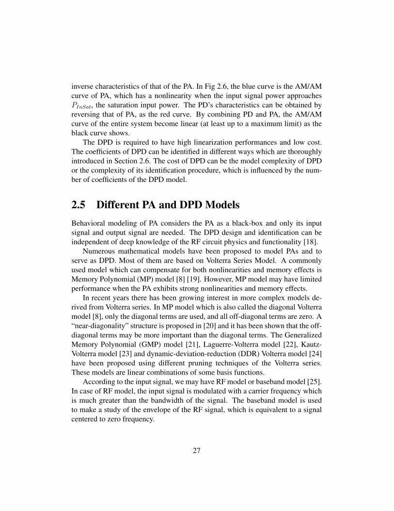
Figure 2.15: Direct Learning Architecture - DLA
2.6.2 Direct Learning ArchitectureThe direct learning architecture (DLA) is depicted in Fig 2.15, where the error tobe minimized is directly the difference between the DPD input and the PA outputnormalized by a reference gain.
The DLA using Nonlinear filtered-x least mean square algorithm (NFxLMS)is proposed in [47]. The model of DPD is estimated according to the PA modeland the reference error ε(n) which is the difference between the DPD input u(n)and the normalized PA output z(n). The coefficient ck of the k-th basis functionΦk[u(n)] could be updated by applying the stochastic gradient algorithm, wherethe gradient is represented by the derivative
∂ε2(n)
∂ck=2ε∗(n)
∂ε(n)
∂ck
=− 2ε∗(n)∂z(n)
∂ck.
(2.40)
Assuming that ck vary slowly, we can have
∂z(n)
∂ck=
L−1∑l=0
∂z(n)
∂x(n− l)· ∂x(n− l)
∂ck
≈L−1∑l=0
∂z(n)
∂x(n− l)· Φk[u(n− l)]
(2.41)
where L is the memory depth of DPD model, and ∂z(n)∂x(n−l) is the derivative of a
nonlinear model of PA normalized by its gain. Thus a model of PA needs to befirstly identified.
40

If we denote g(l, n) = ∂z(n)∂x(n−l) , then (2.41) can be rewritten as
∂z(n)
∂ck≈
L−1∑l=0
g(l, n)Φk[u(n− l)]. (2.42)
It is equivalent that each basis function Φk[u(n)] is filtered by an instantaneousequivalent linear (IEL) filter g(n) = [g(0, n), .., g(L − 1, n)] [50]. Using thismethod, an NFxRLS is proposed for recursive least square (RLS) algorithm. Re-placing (2.42) into (2.40), we can have
∂ε2(n)
∂ck≈− 2ε∗(n)
L−1∑l=0
g(l, n)Φk[u(n− l)]
=− 2[L−1∑l=0
ε(n)g∗(l, n)]∗Φk[u(n− l)]
=− 2[L−1∑l=0
ε(m+ l − L+ 1)g∗(l,m+ l − L+ 1)]∗Φk[u(m− L+ 1)]
(2.43)
if we change the variable m = n− l + L− 1.An adjoint IEL filter gadj(n) = [g∗(L − 1, n), .., g(0, n − L + 1)∗] is then
defined in [50]. It is equivalent that the error signal ε(n) is filtered by the adjointIEL filter. By applying the adjoint IEL for LMS and RLS: Nonlinear adjoint leastmean square algorithm (NALMS) and Nonlinear adjoint recursive least squarealgorithm (NARLS) are proposed in [50]. The computational complexity andmemory requirements are reduced because only the error signal is filtered insteadof every basis function of u(n).
Instead of minimizing the residual between measured output and input sig-nal, Weighted Adjacent Channel Power (WACP) is used in [51] as the objectivefunction to minimize. WACPs represent the distortions in the lower and upperadjacent channel frequencies. It is chosen to avoid the gain/delay compensationerrors and Analog Digital Convertor (ADC) distortion associated with a full timedomain feedback path.
In [52], a closed-loop estimator of DLA is proposed to estimate the DPD coef-ficients. The advantage of this algorithm is that there is no need to identify the PAmodel and the identification of the coefficient errors is solved as a linear problem.Thus it is mainly explained in this section. For models linear with respect to their
41

coefficients, the relation between the input u and the output x of the DPD can beexpressed in matrix form by
x =Uc (2.44)
where x= [x(1), . . . , x(N)]T , c is R× 1 coefficient vector containing the set of ci(i=1,..,R), U isN×Rmatrix of basis functions ΦR[u] whereu= [u(1), . . ., u(N)]T .
The reference error of measurement is calculated by
ε(n) =y(n)
G− u(n) = z(n)− u(n). (2.45)
The origin of the reference comes from two parts:
• The coefficients of DPD are not ideal. As the DPD model is linear with itscoefficients, we can express the error generated by the coefficients error ∆cby U ·∆c, where ∆c is R× 1 vector containing the set of coefficient errors∆ci.
• The LS error εLS in the identification. In LS calculation, QR factorizationis an orthogonal projection. Thus εLS is orthogonal to the input signal U.
Thus the error signal can be also written as
ε = εLS + U ·∆c, (2.46)
To reduce εLS = ε− U ·∆c, we have the cost function to minimize:
J =∑n
|ε(n)−∑k,l
∆ck,l · ΦR[u(n)]|2. (2.47)
The LS solution of the coefficient error which minimize (2.47) is the solution forthe following equation
UHε = [UHU]∆c (2.48)
where ε = [ε(1), . . . , ε(N)]T .With the estimated coefficient error ∆c(i) at i-th iteration, the coefficients are
updated iteratively:
c(i+1) = c(i) − η ·∆c(i) (2.49)
where i indicates the iteration number, 0 < η ≤ 1.In this approach, we do not need to calculate the inverse of the PA model.
42

2.7 Test benchIn order to validate the effectiveness of the proposed algorithms and criteria, ex-periments have been carried out using a test bench. The block diagram and thephoto of the test bench are shown in Fig 2.16 and Fig 2.18 respectively.
PC
Load
VSA
Coupler
AWG
DriverPA
Figure 2.16: Test Bench Blocks Diagram (AWG stands for Arbitrary WaveformGenerator and VSA for Vector Spectrum Analyzer)
The baseband IQ signal is fed from the PC Workstation to the PA chain throughan Arbitrary Waveform Generator (AWG) using a 200 MHz sampling frequency.The AWG up-converts the baseband signal to the carrier frequency. An N5182BMXG X-Series RF Vector Signal Generator is used as AWG (carrier frequencyrange from 9 kHz to 6 GHz).
The signal at the output of the PA is then down-converted to baseband bya Vector Spectrum Analyzer (VSA) which provides to the PC workstation thebaseband signal digitized with a maximum sampling frequency of 200 MHz. A
Driver
(a) Driver in the test bench
Doherty PA
(b) Three-way Doherty PA
Figure 2.17: Three-way Doherty PA and Driver
43

PADriver
VSAAWG
Figure 2.18: Test bench for Experimental Implementation
Rohde & Schwarz FSW signal & spectrum analyzer is used as VSA (receptionfrequency range between 2 Hz and 8 GHz). In this dissertation, the VSA samplingfrequency used is 150 MHz.
The input and output baseband signals are then synchronized in time to beused by the identification algorithm (2.38).
Two PAs have been used to validate the proposed algorithms.The first PA line is made of a three-way Doherty PA designed for base sta-
tion (BS-PA) (Fig 2.17b) with three LDMOS transistors BLF7G22LS-130 fromAmpleon, formerly NXP and its associated driver (Fig 2.17a). This Doherty PAis capable of a peak output power of 57 dBm (500 W) and has a linear gain of16 dB. For most of the experiments in this dissertation, the stimulus signal is anLTE signal with 20 MHz bandwidth and a PAPR of approximately 8 dB, and thecarrier frequency is 2.14 GHz. The modulation of the LTE signal is QPSK.
The nonlinearities and the memory effect of this PA can be seen from theAM-AM/AM-PM curves in Fig 2.19. In this example, the average power of thesignal at the input of the driver is 5 dBm. The linear gain of the driver is 31.5 dB.The measured average output power of DPA is 47.3 dBm, and the measured peakpower is 53.4 dBm. The spectrum of PA output captured by VSA is illustrated inFig 2.20.
The second PA line is made of a Doherty PA designed for broadcast (BrC-PA).Its average output power is 200W. Its normalized AM/AM & AM/PM curves aredepicted in Fig 3.2. The input signal is an OFDM signal with 8 MHz bandwidth
44

Figure 2.19: AMAM & AMPM curves of driver and Doherty PA for an LTE20MHz input signal with 7.8 dB PAPR
and a PAPR of approximately 11 dB, and the carrier frequency is 666 MHz.These measurements have been obtained thanks to the support of National In-
struments on Digital Predistortion Framework research activity [53] and the sup-port of Teamcast in the frame of the ambrun project (FUI AAP11) [54].
The computations described hereafter have been done on an Intel Xeon CPUE3-1245 v3 at 3.40 GHz.
2.8 ConclusionThis chapter introduces the generalities of digital predistortion of power ampli-fiers. The characteristics of PA and the motivation of applying DPD are discussed.Different models can be used as DPD.
The simplest model is a polynomial model which has a deficiency in the per-formance of high power amplifier predistortion with wide bandwidth signals be-cause it cannot compensate for the memory effect. Thus more general Volterraseries model is preferred in the case when memory effects of PA are not negligi-ble. However the complexity of Volterra series model is too high to implement.Hammerstein model and Wiener model are substitutions which compensate for the
45

Figure 2.20: Output signal spectrum of Doherty PA excited by 20MHz bandwidthLTE signal
nonlinearity and the memory effect separately with a reasonable number of terms.For more general performance, Wiener-Hammerstein model is composed by con-catenating these two models together. Memory polynomial model and generalizedmemory polynomial model are proposed to enhance the modeling accuracy witha reasonable increase of model complexity.
To improve DPD performance, some models are proposed by optimizing dif-ferent aspects. The polynomial model can be orthogonalized to improve the per-formance of model coefficient estimation. Vector-switched model and Decom-posed Vector Rotation model are based on vector quantification which may sim-plify the model when the PA characteristics is strongly nonlinear.
Multilayer perceptron neural network is different from the mathematical mod-els above, which can also achieve a good performance in behavioral modeling.
The coefficients of the DPD model can be identified using DLA and ILA. Inthe end of this chapter, the test bench for the experimental implementations in thisdissertation is introduced.
The main contributions of this dissertations are thoroughly presented in thefollowing chapters.
46
Chapter 3
Determining the Structure of DigitalPredistortion Models
3.1 IntroductionVolterra series has good performances in PA or DPD modeling. However its com-plexity is very high. Some models are derived from Volterra series by applyingdifferent pruning techniques. The number of basis functions can be reduced by re-moving those terms which have very few influences on modeling accuracy. Thusan optimal structure of the model which has low complexity while keeping also agood linearization performance is needed.
There are different methods which optimize the structure to have a good trade-off between modeling accuracy and model complexity. Some basis function se-lection techniques to make the model sparse are discussed in this chapter. Anotherway to prune the model is to cut off the basis functions with high orders and deepmemories. Thus some optimization algorithms can be also applied on this prob-lematic to optimize the model dimension. The state of the art is presented in thefollowing sections.
In this chapter we present the first contribution of this dissertation which isan algorithm based on hill-climbing heuristics to determine an optimal modelstructure of DPD according to some criteria. These criteria represent trade-offsbetween modeling accuracy and model complexity. The performance of this algo-rithm is verified on test bench and is compared with other optimization algorithms.The advantage of the proposed algorithm is that its search path can be controlledand some optimizations can then be made to reduce the execution time. The GMP
47

model is taken as an example in the implementations.This chapter is organized as follows:
• Section 2 presents a bibliographic study in model structure optimization.
• The proposed search algorithm based on Hill-Climbing is described in Sec-tion 3.
• In Section 4, we propose two different search criteria for Hill-Climbingheuristic.
• Section 5 presents different pruned neighborhoods to reduce the executiontime.
• In Section 6, two methods to estimate the weighting coefficient of the crite-ria are explained.
• The experimental results are presented and discussed in Section 7.
• Section 8 compares the performances of hill-climbing and genetic algo-rithms.
• Section 9 introduces First-choice hill-climbing which can reduce the execu-tion time while keeping the same performance.
• A brief conclusion is given in Section 10.
3.2 Bibliographic studyBehavioral modeling, which is known as black-box modeling, is a very high levelmodeling as it is based only on the observation of circuit input and output signals.Even with a priori knowledge of the PA internal composition, it is difficult todetermine the structure of a behavioral model which has low complexity and highperformance. There are mainly two methods: selection of basis functions andoptimization algorithms for model structure determination.
48

3.2.1 Basis Functions SelectingThe complexity of model identification using (2.38) and (2.48) depends on thenumber of basis function R. Some pruning technique to reduce the number ofbasis function while keeping the same modeling performance have been studied[55] [56] [57].
An adaptive scheme for selecting basis functions in stochastic conjugate gra-dient (SCG) computations is proposed in [55].
In matrix calculation of SCG, the basis functions are selected according totheir corresponding residual values r = [γ1, · · · , γR]. The residual γi (i=1,..,R)of each basis function fi is defined as the scalar product 1
N(f i · ε) where f i =
[fi(1), · · · , fi(N)], ε is the N -sample error vector. For ILA, the error is the differ-ence between the predistorted signal x(n) and estimated signal zp(n) in Fig 2.14;and for DLA, the error is the difference between the original signal u(n) and thefeedback signal z(n) when DPD is present as in Fig 2.15 [56].
When the residual is negligible, it means the corresponding basis function isnot important and can be omitted. The actual value of residual is registered asthe residual value of that basis function. The average value of the residuals ofthe set of basis functions are set as a threshold. The basis function with residualhigher than the threshold is selected. The SCG uses different sample sets of theinput signal u(n) at different iterations. Thus the threshold is adjusted periodicallyaccording to the new residual calculated in new iterations because the importanceof basis functions varies for different sample sets. In the preconditioned stochasticgradient method (PSGM) proposed in [58] based on SCG, a constraint is added tolimit the change in derivatives from one sample set to another.
The advantage of this adaptive scheme with SCG is that the complexity is re-duced and, at the same time, the convergence rate and the stability of iterationare increased. However this method to calculate the residual of basis functionsis not very stable because the different basis functions present collinearity. Er-ror Variation Ranking (EVR) method has been proposed to alleviate the effect ofcollinearity of basis functions [59].
In EVR method, the importance of a basis function is evaluated by the dif-ference between the modeling performances of DPD model with this basis andwithout this basis. The modeling performance is estimated by the normalizedmean square error (NMSE) value (2.7) between the predicted and measured out-put signals. The basis functions are ranked according to their importances andonly some of the most important basis function will be taken. The NMSE vari-ation caused by removing a basis function is used as quantification factor of its
49

importance. This helps overcoming the problem that potential multicollinearitybetween basis functions of MP model influences the pruning effects on predictionprecision.
In [60], a technique to prune the MP model structure is proposed. The aimis to minimize the number of kernels while the residual between measured signaland predicted signal is kept in a tolerable range. The total number of kernels is de-cided by the nonlinearity order and the memory depth. Assuming that the kernelsolution is sparse, we can keep only few of the coefficients active. The inactivecoefficients are set to zero. The active coefficients of the model is estimated witha maximum likelihood method. With different groups of active coefficients, themodels performances are evaluated. A technique combining Orthogonal Match-ing Pursuit (OMP) method and Bayesian Information Criterion (BIC) is used ascriterion to evaluate their performances. The best model is then determined ac-cording to this criterion.
For a nonparametric identification model, a pruning technique is proposedin [61]. The model structure is not decided a priori. In this case, the character-istic curve of PA is cut into several intervals according to the input amplitude. Astatic nonlinear function is used as the model kernel to describe the curve by av-eraging the amplitude of output samples in each interval. The input signal u(n)is orthogonalized to remove the correlation between u(n) and u(n − l) using theGram-Schmidt (GS) process. With the orthogonalized input matrix, a static non-linear function of each kernel which represents its importance can be calculated.The noncontributing ones are eliminated from the model structure and the model-ing performance can be retained.
3.2.2 Model Structure Optimization AlgorithmsThe model structure with good trade-off between modeling accuracy and modelcomplexity can be also determined by optimization algorithms. There have beenfew studies on sizing nonlinear models in DPD implementation [62] [63] [64][65].
If we take the example of GMP model as (2.16), there are 8 sizing parameters:the nonlinearity orders (Ka, Kb and Kc), and memory depths (La, Lb, and Lc),and the lagging and leading delay tap lengths (Mb andMc). As these parameterscan have their values changed independently, they may compose an 8-dimensiondiscrete space of GMP model structures. An exhaustive search could be used tosize the GMP model but it may be too time consuming. An inadequate numberof basis functions can result in insufficient accuracy or over-fitting problems. The
50

difficulty of sizing GMP model is due to the very large number of different pos-sible model structures. The model basis functions have impacts on each otherbecause of nonorthogonality. New identification of model coefficients is neededeven if only one basis function is added or removed. Adding or removing somebasis functions may have a predictable effect on model complexity, but an uncer-tain influence on modeling accuracy.
For illustration purposes, let us consider the sizing of an MP model which hasonly two sizing parameters: the order of nonlinearity K, and the memory depthL. The basis functions in this case are in the form x(n − l)|x(n − l)|k, wherek ∈ [0,K − 1] and l ∈ [0,L − 1]. If K = 4 and L = 3 and the terms of (k =0, l = 0) and (k = K− 1, l = L− 1) always exist, we have the following possiblearrays of nonlinear orders: {0, 1, 2, 3}, {0, 1, 3}, {0, 2, 3}, {0, 3}, and memorytaps: {0, 1, 2}, {0, 2}. In this case, both full and sparse arrays are consideredsince it may not be necessary to implement all nonlinear orders or delay taps overthe given ranges. Thus there are a total of 8 possible model structures in this case.In general, for each combination of K and L, there are 2K+L−4 possible modelstructures. By increasing the values of K and L, the number of possible solutionswill increase geometrically.
In this chapter we will consider only the discrete space of GMP structures withfull arrays. For the GMP model which has 8 sizing parameters, an exhaustivesearch is very time consuming. For instance if all parameters of the GMP modelare bounded between 1 and 10, there are 108 models to test using exhaustive searchwhen only full arrays are considered, which is very computationally demandingand time consuming.
A general sweep method, in which only full arrays have been considered, hasbeen used to size MP model in [66] and [67]. All possible combinations of Kand L have been evaluated in order to assess the models with different trade-offs between modeling accuracy and complexity. The one which conforms userdemands the most is chosen as the best model. However other models with moresizing parameters, e.g. GMP, cannot be sized with this method. To date, theirparameters are most of the time determined empirically by adjusting one or moreparameter values until the adequate performance is achieved [21] [38] [68]. Andthere is no guarantee that the model found in this way achieves the best trade-offbetween modeling accuracy and complexity.
A search algorithm is needed to find the optimal GMP model structure [62].Optimization algorithms have been widely used in analog electronic domain. Ge-netic Algorithms (GA) have been applied for microwave circuit models [69]. Indigital predistortion, it has been used to identify the coefficients of DPD [70] [71].
51

In the sizing of analog circuits, not only GA [72] [73] but also Particle SwarmOptimization (PSO) [74] have already been shown to be effective. There are alsoa large number of parameters, constraints and performances to handle. Thoughsome studies on optimizing DPD architectures with PSO [63] [64] or with evolu-tionary algorithms in [75] have been done, the DPD models used have much lessparameters to determine than GMP model.
PSO is used to estimate the dimension of MP model DPD in [63]. A systemis proposed to achieve the best trade-off between accuracy and number of zerosin the coefficients’ vector. PSO simulates the social behavior of a particle swarm,e.g. swarm of birds or fish. The particles approach the optimum by iterativelyimproving the candidate solutions according to their positions and velocities.
A method using an integer GA to find the 8 sizing parameters of the GMPmodel has been proposed in [62]. In this algorithm, a fitness function which rep-resents the trade-off between modeling accuracy and structure complexity is usedas a search criterion. Compared with the exhaustive search, a solution close to theoptimal model structure can be found much faster.
Simulated annealing (SA) is another algorithm for optimization problems,which simulates the process of annealing in metallurgy. This method is a meta-heuristic which accepts not only the best solutions in order to overcome the localoptima. The global optimum will be approached if a very long execution timeis allowed. However, the execution time is critical on sizing the model structure,especially when the procedure is implemented in real time.
3.3 Hill-Climbing HeuristicThough PSO and GA are good methods of optimization, it is difficult to controland interpret the path followed by the search algorithm because of its randomnature. Compared with PSO and GA, the advantage of HC is that the search pathcan be controlled by configuring the neighborhood definition. To the best of theauthor knowledge, this is the first time that an algorithm based on Hill-Climbingfor sizing a GMP model DPD structures has been proposed and studied.
Hill-Climbing algorithm [76] [77] is a heuristic which is an iterative algorithmthat begins from an initial solution, then attempts to find a better solution by com-paring the current solution with its neighbors. If there is a better solution amongthe neighbors, it is taken as the new solution. The search procedure repeats untilno better solution can be found.
Instead of exhaustive search, we apply an iterative search (Hill-Climbing al-
52

gorithm [76]) and test only a small number of models in each iteration. The testedmodels in each iteration can be selected in different ways. In this chapter, we se-lect the neighbors of the solution of each iteration to test. The neighbors have alsodifferent definitions because the search space is multi-dimensioned. The algo-rithm depends on two factors: the expression of merit function and the definitionof neighborhood used for search.
In the discrete space U which embodies all different GMP model structures,each element xi can be assigned to a unique structure. The element xi consists of8 integer coordinates: Ka,i, La,i, Kb,i, Lb,i, Mb,i, Kc,i, Lc,i, Mc,i, which are thesizing parameters of the model structure. The value of a merit function J(xi) isassociated to each element xi.
Hill-Climbing heuristic tests only the elements which are the neighbors of thesolution at each iteration. In our implementation, we define a neighbor of elementxi as an 8-tuple (Ka,i + δ1, La,i + δ2, Kb,i + δ3, Lb,i + δ4, Mb,i + δ5, Kc,i + δ6,Lc,i + δ7,Mc,i + δ8), where δ1,...,8 ∈ [0,±1] and δ1,...,8 are not 0 at the same time.The subspace of neighbors is denoted by S, S ⊂ U .
Algorithm 1: Overview of Hill Climbing Heuristic
Set the loop counter q=1;Choose an 8-tuple element x0(1) as the initial element;Evaluate the initial element merit value J(x0(1));xs(0) = x0(1);while (1) do
Compute all J(xi(q)) where xi(q) ∈ S(q);xs(q) = arg minxi(q)∈S(q)
(J(xi(q))
);
if J(xs(q)) < J(xs(q−1)) thenq = q + 1;x0(q) = xs(q−1);
elseend while loop;
endendTake the last solution xs(q) as the best element;
As Algorithm 1 shows, the Hill-Climbing heuristic starts from a given x0(1) atthe first iteration and continually moves in the direction of the element with thebest merit value. At the q-th iteration, the search procedure starts from x0(q) and
53

test the subspace of its neighbors S(q). The neighbors are denoted by xi(q), wherexi(q) ∈ S(q). The merit value J(xi(q)) associated to xi(q) is evaluated. The solutionxs(q) is the element with the minimum merit value among the neighbors.
To simplify the notations, we denote the merit value J(xi(q)) by Ji(q).We compare the merit value of the solution xs(q) with the solution of the pre-
vious iteration xs(q−1). If Js(q) is lower than Js(q−1), at the following iteration, thesearch procedure starts from xs(q) and tests its neighbors. Otherwise the algorithmstops and xs(q) is taken as the final solution. As the neighbors of x0(q) and x0(q+1)
are partially overlapped, i.e. S(q) ∩ S(q+1) 6= ∅, we do not evaluate the elementswhich have been already evaluated at the previous iterations. The search endswhen the solution is not changed in the latest iteration.
3.4 Search CriteriaImproving modeling accuracy by increasing the number of basis functions inducesinevitably an increase in model complexity [56]. Thus the trade-off between mod-eling accuracy and model complexity is a very important criterion for DPD modelselection.
The merit value in our algorithm refers to a certain criterion which leads toa trade-off between modeling accuracy and model complexity. NMSEdB (2.7)can be used to evaluate modeling accuracy. It will be denoted by Y hereafter.The model complexity is represented by the number of coefficients of the model,denoted by R.
We can also take the complexity of model identification instead of model com-plexity as a criterion. The complexity of model identification is in order of R2
if we consider solving (2.38) using a QR decomposition as described in Sec-tion 2.6.1.
In the following sections, NMSEdB, number of coefficients and the merit valueof element xi are denoted by Yi, Ri and Ji respectively.
3.4.1 Weighted Combination of ObjectivesThe aim of combining two objectives into one criterion is for example to find themodel with minimum number of coefficients R while its modeling accuracy Y iskept in a tolerable range.
In [62], a fitness function is defined as a weighted additive combination ofaccuracy and the complexity which is represented by the number of coefficients.
54

In our work, we have considered two different ways to combine Y and R intoa single hybrid criterion: additive and multiplicative combinations.
For the additive combination, the resulting criterion has the same form as in[62] [65]
Ji = Yi + µRi, (3.1)
where µ is a positive real value.For the multiplicative combination
Ji = Yi (1− α ·Ri) (3.2)
which can be rewritten in
Ji = Yi + β(Yi)Ri (3.3)
where β(Yi) = −α · Yi is a dynamic weighting coefficient compared to µ in (3.1).The value of α should respect (1−α ·Ri) > 0. Thus 1
αis the maximum of number
of coefficients.If we take the complexity of model identification for complexity evaluation,
the criteria are kept the same except Ri is replaced by R2i in (3.1) and (3.3).
3.4.2 Additive CriterionWhile comparing two elements xi and xj in the whole space, we denote the dif-ferences of NMSEdB and number of coefficients between xi and xj by ∆Yij and∆Rij respectively:
∆Yij = Yi − Yj∆Rij = Ri −Rj,
(3.4)
For the additive criterion, two elements xi and xj are considered as equivalentif:
Yi + µRi = Yj + µRj
or equivalently Yi − Yj = −µ(Ri −Rj)(3.5)
According to (3.4) and (3.5), we obtain
∆Yij = −µ∆Rij
or∆Yij∆Rij
= −µ.(3.6)
55

We make the trade-off with the additive criterion that an increment of thenumber of coefficients by an amount ∆Rij with Ri > Rj should bring the cor-responding improvement of NMSEdB |∆Yij| equal to or better than µ∆Rij , i.e.|∆Yij| > µ∆Rij . Equivalently, we can say that we accept to degrade the NMSEdB
by an amount ∆Yij = Yi − Yj > 0 if the reduction in number of coefficients|∆Rij| is equal to or better than ∆Yij
µ, i.e. |∆Rij| > ∆Yij
µ.
From (3.6), µ is a constant which represents the NMSEdB tolerance per coef-ficient, or unit tolerance.
3.4.3 Multiplicative CriterionTwo elements xi and xj are considered as equivalent if:
Yi(1− αRi) = Yj(1− αRj) (3.7)
According to (3.4) and (3.7), we have
∆Yij =α (YiRi − (Yi −∆Yij)(Ri −∆Rij))
=α(Yi∆Rij + ∆YijRi −∆Yij∆Rij)
=αYi∆Rij + α∆Yij(Ri −∆Rij).
(3.8)
The normalized variation of NMSEdB is formulated as:
∆YijYi
=∆Rij
1α− (Ri −∆Rij)
. (3.9)
In practical case as we will see in the Section 3.7, the value of 1α
is muchgreater than (Ri − ∆Rij). We can neglect the term (Ri − ∆Rij) and make thefollowing approximation of (3.9) as:
∆YijYi≈ α∆Rij. (3.10)
When |Yi| gets large, the acceptable value of |∆Rij| decreases. In other words,when the modeling is more accurate, we have more requirements on number ofcoefficients.
For example, if α = 0.002, to have an improvement of NMSEdB |∆Yij|=1 dBwhen NMSEdB is around -10 dB, we accept a GMP model with 50 coefficientsmore. When NMSEdB is around -50 dB, we accept a GMP model with only 10coefficients more. The main idea of this criterion is that when the modeling accu-racy is low, we take it as the major factor, and when it is satisfactorily high, wetake the model complexity as the major factor.
56

3.5 Weighting Coefficient DeterminationIn this chapter, we propose two methods to determine the weighting coefficientµ or α: off-line computation and on-line computation, using a sub-space of thediscrete space U of GMP model structures.
As described in previous subsections, µ could be determined by giving certainvalues of ∆Yij
∆Rijin (3.6), and α could be determined by giving directly a certain
percentage value depending on the constraint of the application.And the approach is to consider the global optimum that can be defined in the
following objective as shown in Fig 3.1:
min R, then min Ysubject to Y 6 Yth.
(3.11)
where the threshold Yth is the worst NMSEdB value that we tolerate and its valuedepends on the lowest NMSEdB that a GMP model can reach. If there are morethan one element with the same number of coefficients satisfying the condition,the one with the lowest NMSEdB value is selected. However, it is impossible toknow the lowest NMSEdB for GMP without testing all possible models. Thus thecriteria (3.1) and (3.2) are used to replace (3.11) with correct values of µ or αdetermined by the proposed methods.
If we denote this global optimum by xp, µ or α is determined in order thatthe merit value of xp is better than any other element. Thus, for all elements xn,n 6= p. We have Jn > Jp, which can be written as:
µ(Rn −Rp) > −(Yn − Yp). (3.12)
for the additive criterion, and
α(YnRn − YpRp) 6 Yn − Yp. (3.13)
for the multiplicative criterion.For a certain value of Yth, there is a corresponding µ or α to make the com-
bined criterion (3.1) or (3.2) realize (3.11). Off-line and on-line computation areused to estimate their values by sampling the whole space.
At the q-th iteration, NMSEdB and number of coefficients of element xi(q) aredenoted by Yi(q) and Ri(q) respectively.
As the determinations of µ in (3.1) and α in (3.2) are identical, we explainonly determination of µ in following subsections.
57

Figure 3.1: Global Optimum
3.5.1 Off-line ComputationIn this method, µ is computed off-line before the search with respect to (3.11).
We choose a subset that includes all MP model structures with memory orderKa bounded by Ka 6 Ka,max and memory length La bounded by La 6 La,max.This subset contains Ka,maxLa,max MP structures (which is much smaller than thenumber of GMP structures).
We calculate the NMSEdB for all the elements in this subset. We fix the thresh-old of NMSEdB, Yth, equal to bYmin with bYmin > Ymin = b · Ymin, where Yminis the minimum NMSEdB value obtained for MP models and 0 < b < 1 is a con-stant. For a given b, we get the element xp which has the minimum number ofcoefficients Rp and Yp 6 Yth The element xp, with p ∈ [0,Ka,maxLa,max − 1], isregarded as the best element. µ is determined in order that the merit value of xpis better than any other element. Thus, several inequalities are constructed for allelements xn, with n 6= p. We have Jn > Jp, which gives (3.12).
The estimation of µ is described in Algorithm 2. As (Rn−Rp) can be positiveor negative, we can get an interval of µ. The middle value of the interval will bethen taken as µ for the search in the full space of GMP structures.
58

3.5.2 On-line ComputationIn this method, µ is computed on-line during the search. The chosen subspacesare composed of the GMP models tested at each iteration (at q-th iteration, thesubspace is S(q)). The number of models in the subset at q-th iteration is F(q).
At the first iteration, µ is not estimated and the merit function does not exist.The solution xs(1) is decided by the following steps:
• find Ymin(1)
• select all elements with Y 6 b · Ymin(1)
• find the element with the minimal R among these elements
• then find the element with the minimal Y if multiple elements found in laststep
where Ymin(1) is the lowest Y at the first iteration.To calculate µ, at each iteration, we select a local optimum xp(q) exactly with
the same method as the method described in off-line computation. The only differ-ence is that the subspace here is the neighborhood tested at each iteration insteadof MP models.
Considering xp(q) as the element with the highest merit value in the q-th it-eration, F(q) inequalities as (3.12) are constructed for each element xn(q), withn ∈ [0, F(q)], n 6= p. Thus at each iteration, we can have an interval of µ and wetake the middle value.
On-line computation allows to benefit from a larger sample size than off-linecomputation, the actual µ is updated using a damping factor over the previousvalues by.
µ(q+1) = µ(q) + γ × (µcomputed − µ(q)). (3.14)
The value of γ controls the convergence trend of estimation of µ. When γ istoo large, the value of µ fluctuates much. When γ is too little, the convergencespeed is very slow. In the experiments, a damping coefficient γ = 0.6 is used.
3.6 Pruned NeighborhoodsSince we noticed that the complexity of the algorithm depends on the numberof tested elements, several methods are proposed to reduce the complexity bypruning the neighborhoods.
59

Algorithm 2: Estimation of µ intervalInitialize upper bound ceiling = inf;Initialize lower bound floor = 0;while n ∈ S,Rn 6= Rp do
µ(Rn −Rp) > −(Yn − Yp);µlimit = −(Yn−Yp)
Rn−Rp;
if µlimit ∈ [floor, ceiling] thenif Rn > Rp then
floor = µlimit;else
ceiling = µlimit;end
endend
Literally, the neighborhood refers to the individuals with addresses in the sameregion or nearby. By applying different constraints on neighborhood, the size ofneighborhood can be controlled. To reduce the number of neighbors, we proposedseveral pruned neighborhoods in this section. The constraints can be directly onthe 8 sizing parameters, or on the total number of coefficients.
3.6.1 Constraint on Number of CoefficientsThe numbers of coefficients in the neighbor may have huge variations. We pro-pose a variation limit d for the number of coefficients. In the neighborhoodS(q) of the element x0(q) at q-th iteration, we test only those elements xi(q) with|Ri(q) −R0(q)| 6 d. The set of this constrained neighborhood is denoted by C(q)
and C(q) ⊂ S(q). In this way, we can reduce the number of tests in each iteration.When there is no neighbor element better than x0(q), the search is paused.
In order to keep the algorithm performance, we increment the value of thevariation limit d once the search is paused. The neighborhood is broadened tomake sure that a better element is not missed because of the pruning technique. Interms of complexity, we allow only one increment of d for the same element. Ifno better element is found in the broadened neighborhood after the increment ofd, we take this element as the best solution and the search terminates.
60

3.6.2 Jumping on Number of CoefficientsConsidering thatC(q) still includes many elements, we propose a jumping distances for number of coefficients. In the neighborhood S(q) of the element x0(q) at q-thiteration, we test only those elements xi(q) with |Ri(q) −R0(q)| = s. The set of thisconstrained neighborhood is denoted by D(q) and D(q) ⊂ C(q).
The algorithm will move forward by jumping over a large amount of elements,which makes it converge to the global optimum very fast.
With the same idea, once the algorithm is stuck at an element, we incrementthe value of the jumping distance s to detect if there are better elements in thebroadened neighborhood. This increment is applied only one time for one solu-tion. When the search terminates, we take the current solution as the final solution.
3.6.3 Unidimensional neighborThe pruning technique can be also applied on the sizing parameters. In the con-ventional neighborhood definition, all the parameters of a neighbor of element xican have a variation of ±1. Thus in case of 8 parameters, the maximum size ofneighborhood is 38 − 1.
To reduce the size of neighborhood, we propose to limit the the number ofvaried parameters to one. The neighbors of xi have parametersKa,i+δ1, La,i+δ2,Kb,i+ δ3, Lb,i+ δ4,Mb,i+ δ5, Kc,i+ δ6, Lc,i+ δ7,Mc,i+ δ8, where
∑8i=1 |δi| = 1.
The number of neighbors of an element decreases sharply to 16.This definition of neighborhood is called unidimensional neighborhood while
the conventional one without constraint is called full-dimensional neighborhood.This helps the search path to converge to the region of the global optimum withvery few tested models.
Once the search path is stuck at an element, we will remove this constraintand test its full-dimensional neighbors. If no better element is found, we take thecurrent solution as the final solution.
3.7 Experiments and Results
3.7.1 Experimental Signal AcquisitionAs indicated in Chapter 2, two PAs have been used to validate the proposed al-gorithm. The first PA line is made of the Doherty PA (Fig 2.17b) introduced inChapter 2, which is designed as a base station PA (BS-PA).
61

Figure 3.2: AMAM & AMPM curves of Doherty Broadcast PA
The second PA line is made of a Doherty Broadcast PA. The measured dataof this PA were provided by Teamcast group. Its normalized AM/AM & AM/PMcurves are depicted in Fig 3.2.
The input and output baseband signals are synchronized in time to be used bythe identification algorithm (2.38).
The following subsections present the experimental results.For each PA, base station (BS-PA) and broadcast (BrC-PA), the results searched
with the following criteria are presented:
1. the additive criterion with µ determined off-line (ACoff)
2. the additive criterion with µ determined on-line (ACon)
3. the multiplicative criterion with α determined off-line (MCoff)
4. the multiplicative criterion with α determined on-line (MCon)
In each result, there are two different implementations of the search algorithm:the first implementation (1-step) is to search the best GMP model from the verybeginning; and the second implementation (2-step) is divided into two steps: firstwe find out the MP model minimizing the search criterion; then we start from thisMP model, to find the best GMP model.
62

The 1-step search starts from the element which corresponds to the linear func-tion yGMP (n) = ax(n) where
Ka =1,La = 1
Kb =0,Lb = 1,Mb = 1
Kc =0,Lc = 1,Mc = 1.
(3.15)
In our searches, we estimate µ and α with b = 97% in (3.11). We restrict theparameters to the following intervals:
1 6 Ka 6 11, 1 6 La 6 5
0 6 Kb 6 10, 1 6 Lb 6 5, 1 6Mb 6 4
0 6 Kc 6 10, 1 6 Lc 6 5, 1 6Mc 6 4,
(3.16)
with a global constraint on the total number of coefficients R < 80. Each GMPmodel is identified using 15000 samples.
In off-line computation, the interval of µ or α is determined as described inSection 3.5, with Ka,max = 11 and La,max = 11.
In on-line computation, the interval of µ or α is computed with the testedelements at every iteration. The middle of the interval is taken to renew the valueof µ or α.
3.7.2 Exhaustive SearchIn order to evaluate our proposed criteria (3.1) and (3.2), we have conducted an ex-haustive search as a reference to get all (Y,R) couples. Inspection of these resultsallows to determine the best GMP model (i.e. minimum number of coefficients)for a given NMSEdB requirement.
For the BS-PA, the lowest NMSEdB is -33.91 and is obtained with 79 coef-ficients. As shown in Fig 3.3, we have the threshold bYmin=-32.90 dB in (3.11)with b = 0.97. From that we get xp = (Y,R) = (−32.96, 43) with structure
Ka =11,La = 2
Kb =1,Lb = 3,Mb = 3
Kc =3,Lc = 4,Mc = 1.
(3.17)
For the BrC-PA, the lowest NMSEdB is -41.79 also with 79 coefficients. Wehave the threshold bYmin=-40.54 dB. From that we get xp = (Y,R) = (−40.56, 28)
63

Figure 3.3: Determination of upper bound and lower bound of µ with a concaveedge
with structure
Ka =9,La = 2
Kb =1,Lb = 1,Mb = 1
Kc =3,Lc = 3,Mc = 1.
(3.18)
In the following paragraph we will use the results of the exhaustive search tocompute reference values for µ and α as described in Section 3.5.1. Consideringxp as the element with the best merit value, we can construct inequalities as (3.12)or (3.13) to determine an interval for µ or α.
Here we take the estimation of µ as an example.From (3.11) and (3.12), we have
µ > − Yn − YpRn −Rp
= µfloor (3.19)
for Rn > Rp. The interval of µ is given [µfloor, inf[.We can also set an upper bound. Let us consider the entire space. As xp is the
best element, we should have Jp 6 Jm where Rm < Rp and Ym > Yp (there is noelement xm with Rm < Rp and Ym < Yp, otherwise this xm is taken as xp). Thus
64

Figure 3.4: Determination of upper bound and lower bound of µ with a concaveedge
we have
µ 6 − Ym − YpRm −Rp
= µceiling. (3.20)
In this way we can have a refined interval of µ: [µfloor, µceiling].However as our search space is discrete, the edge of the blue cloud in Fig 3.3
can be concave. For instance, in Fig 3.4, if we define a such value of µ that xp andx1 have the same merit value, we can plot a curve passing by these two points withslope equal to µ. The lower bound µfloor = 0.08 is determined by xp and x1, andthe upper boundµceiling = 0.05 is determined by xp and x2. From the inspectionof Fig 3.4 we can see that xp lies in a concave region of the edge. This will resultin an empty interval for µ.
In this case we can observe that µ can be approximated to the slope of thedashed line passing by x1 and x2. Thus with the signal of the BS-PA, we take0.055 for the value of µ.
For the multiplicative criterion, the upper bound is 1.4e−3, and the lowerbound is 2.2e−3. In the same way, we take finally 1.5e−3 for the value of α.
The GMP model space is represented into 3-D. The merit values are given infunction of NMSEdB value, number of coefficients and the merit value in Fig 3.5.
65

Figure 3.5: BS-PA: Exhaustive search results in function of NMSEdB and numberof coefficients in 3D
With the signal of the BrC-PA, we get an interval of µ equal to [0.0823, 0.0927]for the additive criterion. The mean value µ = 0.0875 is taken.
For the multiplicative criterion, we get an interval of α equal to [1.9e−3, 2.2e−3].The mean value α = 2e−3 is chosen.
We denote the element with the lowest merit value Jmin by Xmin. The impactof different values of µ and α in the intervals on the algorithm performances andon Xmin is shown in Tables 3.1-3.4, where SolNMSE, SolNb, NMSEXmin
andNbXmin
are the NMSEdB value and number of coefficients of the solution found bythe algorithm and Xmin respectively. For base station PA, the solution and Xmin
at the upper limit of interval of µ and α have more coefficients and also have betterNMSEdB. For broadcast PA, both the solution and Xmin are not sensitive to thevalues of µ and α in these intervals.
3.7.3 Test with Doherty PA for Base StationHill-Climbing heuristic using Off-line additive criterion (ACoff)
In 1-step search, we determine µ with the subspace of MP models before theGMP model search. The interval of µ is [0.039, 0.070]. If we choose the mean
66

Table 3.1: Additive criterion with different µ for BS-PA
SolNMSE: NMSEdB value of the solution found by the algorithmSolNb: The number of coefficients of the solution found by the algorithmNMSEXmin
: NMSEdB value of Xmin
NbXmin: The number of coefficients of Xmin
µ SolNMSE SolNb NMSEXminNbXmin
0.050 -32.96 43 -33.04 440.055 -32.71 38 -33.04 440.060 -32.71 38 -32.71 380.065 -32.71 38 -32.71 380.070 -32.65 37 -32.65 370.075 -32.65 37 -32.65 370.080 -32.65 37 -32.65 37
Table 3.2: Multiplicative criterion with different α for BS-PA
α SolNMSE SolNb NMSEXminNbXmin
1.4e−3 -32.96 43 -33.04 441.5e−3 -32.70 38 -33.04 441.6e−3 -32.70 38 -32.71 381.7e−3 -32.70 38 -32.71 381.8e−3 -32.71 38 -32.71 381.9e−3 -32.71 38 -32.71 382.0e−3 -32.65 37 -32.65 372.1e−3 -32.65 37 -32.65 372.2e−3 -32.65 37 -32.65 37
67

Table 3.3: Additive criterion with different µ for BrC-PA
µ SolNMSE SolNb NMSEXminNbXmin
0.082 -38.50 18 -40.64 290.084 -38.50 18 -40.56 280.086 -38.50 18 -40.56 280.087 -38.50 18 -40.56 280.088 -38.50 18 -40.56 280.090 -38.50 18 -40.56 280.092 -38.50 18 -40.56 28
Table 3.4: Multiplicative criterion with different α for BrC-PA
α SolNMSE SolNb NMSEXminNbXmin
1.9e−3 -38.50 18 -40.64 292.0e−3 -38.50 18 -40.56 282.1e−3 -38.50 18 -40.56 282.2e−3 -38.50 18 -40.37 26
value which is 0.055, the final solution, Sol in Fig 3.6, given by the algorithm is(Y,R) = (−32.71, 38). The structure found is
Ka =11,La = 2
Kb =4,Lb = 1,Mb = 1
Kc =3,Lc = 4,Mc = 1.
(3.21)
In this search, there are totally 10821 different GMP models tested in 11 iterations.The execution time is 15.85 minutes. The searching iterations are indicated inFig 3.6.
The iterations in function of Y (NMSEdB) and R (Nb of Coeff) are depicted inFig 3.6. The results of the exhaustive search are the background blue points (samefor the following figures). The solutions of successive iterations are indicated bycircles. The best element Xmin according to the criterion (3.1) with µ = 0.055has 44 coefficients with NMSEdB of -33.04 dB.
In Fig 3.6, the elements of the neighborhood tested in each iteration are shownin different colors. The point with an arrow “1” is the initial element x0(1). Thepoints around with the same color are the neighbors of this element. The otherblack circles shows the best elements picked among their neighbors as the solution
68

Figure 3.6: BS-PA: search path of Hill-Climbing heuristic with off-line additivecriterion (µ = 0.055)
at each iteration.The evolution of the algorithm is depicted in Fig 3.7 for the first two iterations.
In Fig 3.7a, the red points are neighbors of x0(1), which are tested at the firstiteration. Then the black circle “2” is selected as the solution xs(1). In Fig 3.7b,the purple points are neighbors of xs(1), which are tested at the second iteration,and the circle “3” is selected as xs(2). We can see that the search path convergestowards the lowest merit value which corresponds to the best structure given asXmin. As each element will be tested at most only once, there is no overlapbetween the red points and the purple points.
With the same method to determine µ, the two-step implementation (ACoff2)firstly searches only MP models, and then searches GMP models from the MPmodel solution. in the first step, there are 39 different MP models tested in 11iterations during 3.6 seconds. The structure of the MP model with the best meritvalue found is Ka = 11, La = 3 with NMSEdB of -31.56 dB. And in the secondstep, starting from the element where Ka = 11, Kb = 0, Kc = 0, La = 3, Lb = 1,Lc = 1,Mb = 1,Mc = 1, there are 7037 different GMP model structures testedin 4 iterations during 12.64 minutes. The search path is depicted in Fig 3.8. The
69

(a) BS-PA: Neighborhood of the initial solution
(b) BS-PA: Neighborhood of the 2nd iteration
Figure 3.7: BS-PA: Neighborhoods demonstration of Hill-Climbing heuristic withadditive criterion (µ = 0.055)
70

Figure 3.8: BS-PA: Two-step search path of Hill-Climbing heuristic with Off-lineadditive criterion (µ = 0.055)
best structure Xmin found by the algorithm is
Ka =11,La = 2
Kb =1,Lb = 4,Mb = 1
Kc =3,Lc = 3,Mc = 2.
(3.22)
which has 44 coefficients and its NMSEdB value is -33.04 dB.Using the additive criterion when µ determined with off-line computation, 2-
step search can reduce the number of tests and execution time. As there are muchless MP models than GMP models, by searching the best MP model, ACoff2converges to Xmin with only a few tests. Here Xmin is evaluated with criterion(3.1) with µ = 0.055. The GMP search step has only 4 iterations in Fig 3.8 insteadof 11 iterations in Fig 3.6. The 2-step search avoids many tests in the zones whichare not the neighborhood of Xmin.
Hill-Climbing heuristic using On-line additive criterion (ACon)
As mentioned before, in ACon, µ is determined with the subspace discovered ateach iteration and its value is renewed according to (3.14). The evolution of the
71

Table 3.5: BS-PA: Evolution of µ
No. It 1 2 3 4 5 6µ 0 0.242 0.176 0.163 0.148 0.116No. It 7 8 9 10 11µ 0.107 0.086 0.075 0.058 0.055
Table 3.6: BS-PA: Evolution of µ in Two Steps
No. It 1 2 3 4µ 0 0.711 0.688 0.694
(a) MP search step
No. It 1 2 3 4µ 0.829 0.139 0.112 0.105No. It 5 6 7 8µ 0.085 0.075 0.057 0.055
(b) GMP search step
value of µ is shown in Table 3.5. The value of µ converges towards the referencevalue 0.065 and becomes stable after 8 iterations.
In this search, the algorithm has 11 iterations and there are totally 8539 differ-ent GMP model structures tested during 12.78 minutes. The iterations in functionof Y (NMSEdB) and R (Nb of Coeff) are depicted in Fig 3.9. The solutions of it-erations are indicated by circles with annotations. We can see that the search pathconverges towards the lowest merit value which corresponds to the best structuregiven as Xmin. Here Xmin, the same as (3.22), is evaluated based on the latestvalue of µ which is 0.055. According to all these (Y , R) couples, we found thesolution the same as (3.21) which has 38 coefficients and NMSEdB of −32.71 dB.
In 2-step search (ACon2), with the same method to estimate µ, we can reachthe best element in 12 iterations. The evolution of the value of µ is shown inTable 3.6. With the final value µ = 0.055, Xmin given by the criterion (3.2) has44 coefficients with NMSEdB equal to -33.04 dB, and its structure is the same as(3.22).
72

Figure 3.9: BS-PA: On-line additive criterion in function of NMSEdB and numberof coefficients (µ = 0.055)
In the first step, there are 15 different MP models tested in 4 iterations during0.649 seconds. The structure of the MP model with the best merit value found isKa = 4, La = 2 with NMSEdB of -25.88 dB. In the second step, starting from theelement where Ka = 4, Kb = 0, Kc = 0, La = 2, Lb = 1, Lc = 1, Mb = 1,Mc = 1, there are 8155 different GMP model structures tested in 8 iterationsduring 12.58 minutes. The search path is depicted in Fig 3.10. The blue points areagain the exhaustive results, and the circles with annotations are the solutions ofiterations in the Hill-Climbing heuristic. The best structure found by the algorithmis also (3.21).
Comparing ACon2 with ACon, we can see that, 2-step search does not reducethe number of tests and execution time in on-line computation as it did in off-line computation. That is due to the inaccurate determination of µ during the firststep. In MP model search, we tested only 15 MP models in 4 iterations. In otherwords, less than 4 models in average are used to determine µ at each iteration.Determining the value of µ with these small size sampling sometimes get a resultfar from its final converged value, which can be seen in Table 3.6. Thus in thiscase the first step does not improve the algorithm.
73

Figure 3.10: BS-PA: Two-step search path of Hill-Climbing heuristic with On-lineadditive criterion (µ = 0.055)
Furthermore with the on-line computation, we can see that the search pathfollows the envelop of the blue points cloud, which can reduce the computationcomplexity. Further discussions are presented in Section 3.7.5.
Hill-Climbing heuristic using Off-line multiplicative criterion (MCoff)
Using the MP models subspace, the interval for α is [0.0012, 0.0021] and the meanvalue 1.7e−3 has been chosen. With this α, the best element Xmin given by thecriterion is the same as (3.21).
In 1-step search, the algorithm has 11 iterations and there are totally 19598different GMP model structures tested. The iterations in function of Y (NMSEdB)and R (Nb of Coeff) are depicted in Fig 3.11. The solutions of iterations areindicated by circles with annotations. We can see that the search path convergestowards the lowest merit value which corresponds to the best structure given asXmin which is (3.21). The execution time is 29.89 minutes.
In two-step search (MCoff2), in the first step, there are 39 different MP modelstested in 11 iterations during 3.6 seconds. The structure of the MP model withthe best merit value found is Ka = 11, La = 3 with NMSEdB of -31.13 dB. In
74

Figure 3.11: BS-PA: Off-line multiplicative criterion in function of NMSEdB andnumber of coefficients (α = 1.7e−3)
the second step, starting from the element where Ka = 11, Kb = 0, Kc = 0,La = 3, Lb = 1, Lc = 1, Mb = 1, Mc = 1, there are 7364 different GMPmodel structures tested with 4 iterations during 14.20 minutes. The search path isdepicted in Fig 3.12. The solution found by the algorithm is the same as (3.22)which has 44 coefficients and its NMSEdB value is -33.04 dB.
The value of α estimated by off-line computation, 1.7e−3, is close to the refer-ence value, 1.8e−3. Comparing with MCoff, we can see that MCoff2 reduces thenumber of tests and execution time with a solution close to the optimum.
Hill-Climbing heuristic using On-line multiplicative criterion (MCon)
Using the subspace composed of the models tested at each iteration, we can de-termine α dynamically.
In 1-step search, the algorithm has 13 iterations and there are totally 12692different GMP model structures tested during 17.12 minutes. The evolution of thevalue of α is shown in Table 3.7.
Xmin given by the criterion (3.2) with α = 0.0016 is the same as (3.22). Theiterations in function of Y (NMSEdB) andR (Nb of Coeff) are depicted in Fig 3.13.
75

Figure 3.12: BS-PA: Two-step search path of Hill-Climbing heuristic with Off-line multiplicative criterion (α = 1.7e−3)
Table 3.7: BS-PA: Evolution of α
No. It 1 2 3 4 5α 0 11.7 0.0079 0.0064 0.0054No. It 6 7 8 9 10α 0.0038 0.0034 0.0027 0.0022 0.0024No. It 11 12 13α 0.0019 0.0017 0.0016
76

Figure 3.13: BS-PA: On-line multiplicative criterion in function of NMSEdB andnumber of coefficients (α = 1.6e−3)
According to all these (Y , R) couples, the algorithm found the best structure with44 coefficients having NMSEdB of −33.04 dB as (3.22).
In two-step search (MCon2), the best element is reached in 12 iterations. Inthe first step, there are 15 different MP models tested in 4 iterations during 1.7138seconds. The evolution of the value of α is shown in Table 3.8. Xmin given by thecriterion (3.1) with α = 1.6e−3 is the same with (3.22).
The structure of the MP model with the best merit value found is Ka = 4,La = 2 with NMSEdB of -25.88 dB. In the second step, starting from the elementwhere Ka = 4, Kb = 0, Kc = 0, La = 2, Lb = 1, Lc = 1,Mb = 1,Mc = 1,there are 12692 different GMP model structures tested in 10 iterations during18.31 minutes. The search path is depicted in Fig 3.14. The best structure foundby the algorithm is the same as (3.22) which has 44 coefficients and its NMSEdB
value is -33.04 dB.The first step of the algorithm does not help reducing the execution time be-
cause the determination of α decays with very small number of MP models. Thefinal result is the same with MCon.
77

Table 3.8: BS-PA: Evolution of α in Two Steps
No. It 1 2 3 4α 0 0.0169 0.0219 0.0220
(a) MP search step
No. It 1 2 3 4 5α 0.0262 0.0048 0.0038 0.0034 0.0027No. It 6 7 8 9 10α 0.0022 0.0024 0.0019 0.0017 0.0016
(b) GMP search step
Figure 3.14: BS-PA: Two-step search path of Hill-Climbing heuristic with On-linemultiplicative criterion (α = 1.6e−3)
78

3.7.4 Test with Doherty PA for BroadcastHill-Climbing heuristic using Off-line additive criterion (ACoff)
The estimated interval of µ is [0.163, 0.263] with MP model subspace, and wetake the mean µ = 0.213 which is outside the reference interval. In this case wefound that the determined value of µ is much different from the reference valueµ = 0.0875 in Section 3.7.2. As the sample size of off-line computation is notlarge enough, the estimation is not always accurate.
In 1-step search, we can find a solution in 5 iterations. There are totally 4608GMP model structures tested. The search path is depicted in Fig 3.15. Xmin givenby the criterion (3.1) with µ = 0.213 has 15 coefficients and NMSEdB value of-38.7473 dB, and its structure is
Ka =8,La = 1
Kb =1,Lb = 1,Mb = 1
Kc =2,Lc = 3,Mc = 1.
(3.23)
The search path ends at the point with a distance of (3,−1.22dB) from to Xmin
which is the best GMP model structure according to the additive criterion. Theparameters of the final solution are:
Ka =5,La = 1
Kb =1,Lb = 1,Mb = 1
Kc =2,Lc = 3,Mc = 1
(3.24)
with NMSEdB of -37.52 dB and 12 coefficients. The execution time is 4.50 min-utes.
Using 2-step approach (ACoff2), first we find the MP model (Ka = 4,La = 2)with NMSEdB of -32.82 dB. In this step, 14 MP model structures are tested in 4iterations during 1.28 seconds. From this MP model, we can find a GMP modelstructure as the final solution with 3 iterations, and 3606 GMP model structuresare tested during 3.47 minutes. The final solution is the same as (3.24) withNMSEdB of -37.52 dB and 12 coefficients. In Fig 3.16 we can see that the searchpath ends at the point with a distance of (3,−1.22dB) from the star Xmin whichis the same as (3.23).
Hill-Climbing heuristic using On-line additive criterion (ACon)
In 1-step search, with the additive criterion, we can find a solution in 5 iterations.There are totally 6168 GMP model structures tested during 6.41 minutes. The
79

Figure 3.15: BrC-PA: search path of Hill-Climbing heuristic with Off-line additivecriterion (µ = 0.213)
search path is depicted in Fig 3.17. The final solution which is the same as
Ka =5,La = 2
Kb =1,Lb = 1,Mb = 1
Kc =3,Lc = 2,Mc = 1
(3.25)
which has 17 coefficients and NMSEdB of -38.20 dB.It has a distance of (4,−1.69dB) to Xmin which is the best GMP model struc-
ture according to the additive criterion. Here Xmin evaluated based on the latestvalue µ = 0.1416 has 21 coefficients and NMSEdB of -39.89 dB. The structure ofXmin is
Ka =4,La = 1
Kb =1,Lb = 1,Mb = 1
Kc =8,Lc = 2,Mc = 1.
(3.26)
The evolution of the value of µ is shown in Table 3.9.Using 2-step approach (ACon2), first we find the MP model (Ka = 5,La = 2)
with NMSEdB of -33.16 dB. In this step, 14 MP model structures are tested in 4
80

Figure 3.16: BrC-PA: Two-step search path of Hill-Climbing heuristic with Off-line additive criterion (µ = 0.213)
Table 3.9: BrC-PA: Evolution of µ
No. Iter 1 2 3 4µ 0 0.0686 0.2150 0.1954No. Iter 5 6 7µ 0.1933 0.1923 0.1416
81

Table 3.10: BrC-PA: Evolution of µ in Two Steps
No. It 1 2 3 4µ 0 0.0775 0.1223 0.1309
(a) MP search step
No. It 1 2 3µ 0.0883 0.2781 0.2199
(b) GMP search step
iterations during 1.28 seconds. From this MP model, a GMP model structure asthe final solution is found with 3 iterations, and 2856 GMP model structures havebeen tested during 2.91 minutes. This final solution is the same as (3.24) with 12coefficients and NMSEdB of -37.52 dB.
In Fig 3.18 we can see the solution of the search path has a distance of (9,−2.48dB)to the star which represents Xmin. Here Xmin evaluated based on the latest valueµ = 0.2199 is the same as (3.23).
The evolution of the value of µ is shown in Table 3.10.
Hill-Climbing heuristic using Off-line multiplicative criterion (MCoff)
With the Off-line multiplicative criterion, the interval of α is [0.0077, 0.0047], andwe take the mean α = 6.2e−3.
In 1-step search, the solution is found in 5 iterations. There are totally 3056GMP model structures tested. The search path is depicted in Fig 3.19. This finalsolution as
Ka =5,La = 1
Kb =1,Lb = 1,Mb = 1
Kc =2,Lc = 2,Mc = 1
(3.27)
with NMSEdB of -37.04 dB and 10 coefficients. It approaches Xmin which isthe best GMP model structure according to the multiplicative criterion with α =6.2e−3. Here Xmin is the same as (3.23). The execution time is 2.66 minutes.
Using 2-step approach (MCoff2), first we find the MP model (Ka = 4,La = 2)with NMSEdB of -32.82 dB. In this step, 14 MP model structures are tested during
82

Figure 3.17: BrC-PA: search path of Hill-Climbing heuristic with On-line additivecriterion (µ = 0.1416)
2.35 seconds. From this MP model, we can find a GMP model structure as thefinal solution with 3 iterations, and 2568 GMP model structures are tested during2.66 minutes. The final solution is the same as (3.27) and Xmin is the same as(3.23). In Fig 3.20 we can see the search path and it ends at the point with adistance of (3,−1.22dB) from the star which represents Xmin which is evaluatedby the multiplicative criterion with α = 6.2e−3.
Hill-Climbing heuristic using On-line multiplicative criterion (MCon)
In 1-step search, with the multiplicative criterion, we can find a solution in 5 iter-ations. There are totally 3820 GMP model structures tested during 3.41 minutes.The search path is depicted in Fig 3.21. The final solution is the same as (3.24).Here Xmin evaluated based on the latest value of α which is 0.0050 is the same as(3.23).
The evolution of the value of α is shown in Table 3.11.Using 2-step approach (MCon2), first we find the MP model (Ka = 4,La = 2)
with NMSEdB of -32.83 dB. In this step, 15 MP model structures are tested in 4iterations during 1.79 seconds. From this MP model, we can find a GMP model
83
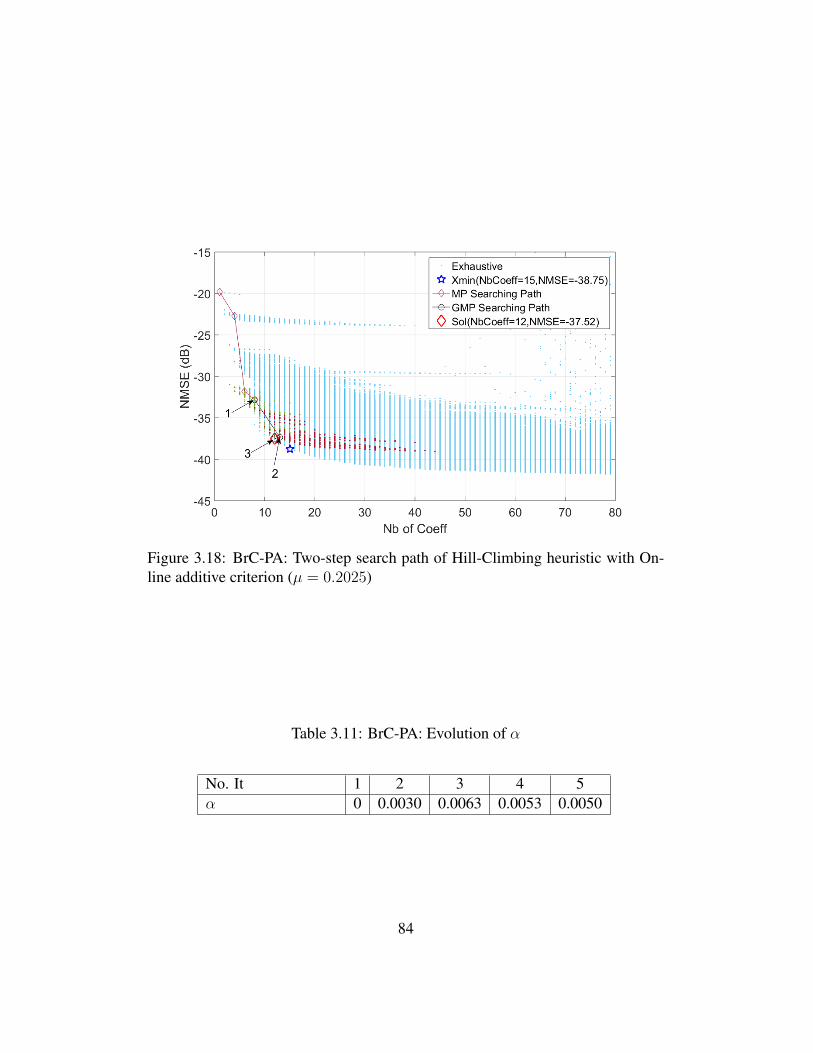
Figure 3.18: BrC-PA: Two-step search path of Hill-Climbing heuristic with On-line additive criterion (µ = 0.2025)
Table 3.11: BrC-PA: Evolution of α
No. It 1 2 3 4 5α 0 0.0030 0.0063 0.0053 0.0050
84

Figure 3.19: BrC-PA: search path of Hill-Climbing heuristic with Off-line multi-plicative criterion (α = 6.2e−3)
structure as the final solution with 4 iterations, and 3000 GMP model structuresare tested during 3.09 minutes. The final solution is the same as (3.24).
In Fig 3.22 we can see the search path which ends at the point with a distanceof (3,−1.22dB) from the star which representsXmin. HereXmin evaluated basedon the latest value of α = 0.0038 is the same as (3.23).
The evolution of the value of α is shown in Table 3.12.
3.7.5 DiscussionFor the exhaustive results which are depicted by the light blue point cloud inFig 3.5 - Fig 3.22, the left and lower edge of the point cloud is defined as itsenvelop. The slope of this envelop is steep on the left edge and flat on the loweredge. The connection of these two edges is the turning area where the slopedecreases prominently. For broadcast PA, e.g.
The normalized execution times show the comparative complexities of differ-ent search procedures. The total execution time of ACoff (search plus off-linedetermination of µ, which lasts 15.85 minutes in case of base station PA and 4.50
85

Figure 3.20: BrC-PA: Two-step search path of Hill-Climbing heuristic with Off-line multiplicative criterion (α = 6.2e−3)
Table 3.12: BrC-PA: Evolution of α in Two Steps
No. It 1 2 3 4α 0 0.0017 0.0035 0.0038
(a) MP search step
No. It 1 2 3 4α 0.0062 0.0060 0.0051 0.0038
(b) GMP search step
86

Figure 3.21: BrC-PA: search path of Hill-Climbing heuristic with On-line multi-plicative criterion (α = 5e−3)
minutes in case of broadcast PA) is taken as the unit time. The complexity is rep-resented by the execution time and the number of tested model which are providedin the Tables summarizing the performances of the different implementations.
The exhaustive search covers all possible models with R < 80. So Xmin canbe regarded as the global optimum. Though using Hill-Climbing heuristic cannot always reach Xmin, as sometimes it seems stuck at a local optimum when thesearch path does not reach Xmin or its neighbors, e.g. Fig 3.19 and Fig 3.20, it isstill a reliable method to size the GMP models. The results show that the searchpath starts from the simplest model straightly towards the global optimum. Andwe can observe that the found solution is most of the time very close to the globaloptimum and located on the envelop.
Both the additive criterion and the multiplicative criterion achieve a good per-formance. For the signal of base station PA, the search with additive criterion takesless execution time than the multiplicative criterion. For the signal of broadcastPA, the multiplicative criterion has advantage on execution time.
According to the results, the velocity of algorithm convergence depends mainlyon two factors: the number of tested models and the complexity of tested models.
87

Figure 3.22: BrC-PA: Two-step search path of Hill-Climbing heuristic with On-line multiplicative criterion (α = 3.8e−3)
Table 3.13: Comparison of GMP Results of Different Searches with BS-PA
ACoff ACoff2 ACon ACon2NMSEdB -32.71 -33.04 -32.71 -32.71NbCoeff 38 44 38 38Nb of Test 10821 39+7037 8539 15+8155Nb of Iter 11 11+4 11 4+8Ex. Time 1 0.80 0.81 0.79
MCoff MCoff2 MCon MCon2NMSEdB -32.71 -33.04 -33.04 -33.04NbCoeff 38 44 44 44Nb of Test 19598 39+7364 12692 15+12692Nb of Iter 11 11+4 13 4+10Ex. Time 1.89 0.90 1.08 1.16
88

Table 3.14: Comparison of GMP Results of Different Searches with BrC-PA
ACoff ACoff2 ACon ACon2NMSEdB -37.52 -38.75 -38.20 -37.52NbCoeff 12 15 17 12Nb of Test 4608 14+3606 6168 14+2856Nb of Iter 5 4+3 7 4+3Ex. Time 1 0.77 1.42 0.65
MCoff MCoff2 MCon MCon2NMSEdB -37.04 -37.04 -37.52 -37.52NbCoeff 10 10 12 12Nb of Test 3056 18+2568 3820 14+3000Nb of Iter 5 5+3 5 4+4Ex. Time 0.59 0.56 0.76 0.69
From Table 3.13 and Table 3.14, we can see that the number of tested models hasimpact on the execution time, but not in a proportional way. For example in Table3.13 ACoff has 25406 GMP models tested during 39.91 minutes while ACoff2 has10130 GMP models tested during 19.99 minutes. The average execution time permodel of ACoff2 (which is 0.1184 s/model) is greater than that of ACoff (whichis 0.0943 s/model). That is because ACoff2 starts to search GMP models from anelement which has high order of nonlinearity and/or deep memory depth and theneighbors of this element have very large number of basis functions.
The points on the envelop correspond to the GMP models with the simpleststructure among those of the same NMSEdB value. When the path follows theenvelop, the tested models have less complexity compared with models which arenot on the envelop. When it follows the envelop as in Fig 3.19 than having zigzagshapes, e.g. in Fig 3.11 or in Fig 3.20, the search path has less average executiontime.
The determination of weighting coefficients is a challenge in construction ofmerit functions. According to (3.11), the final solution should have the least num-ber of coefficients while its NMSEdB is better than bYmin. With the estimationmethods proposed in this chapter, we can restrict the weighting coefficient to agiven range. On-line computation allows to refine the value of weighting coeffi-cient as it has more samples for the estimation.
With the signal of the broadcast PA, the final solutions found by the algo-rithms are not located exactly at but very close to the points of Xmin. The search
89

path stops at the local optimum after approaching the zone where the values ofNMSEdB get stable.
The broadcast PA can be well modeled by a GMP model with low nonlinearityorder and memory depth (NMSEdB <-37 dB). Thus we can see that the envelopfalls down very fast when R < 10 in Fig 3.15-3.22. When R > 20 we can see thatthe envelop is stable in terms of NMSEdB. The area 10 < R < 20 is the turningarea. Once a model in this area is reached, we need to add much more coefficientsto have the same improvement of modeling accuracy.
For the algorithms with weighting coefficients determined with off-line method,2-step search always reduces the number of tests and execution time for both PAs.The search for the best MP model is faster because an MP model has much fewerneighbors than a GMP model. Starting from the linear memoryless model, MPmodel search reaches a region towards the best element rapidly, e.g. Fig 3.8.
For the algorithms with weighting coefficients determined with on-line com-putation, the advantage of 2-step search is very limited. The tested models in thefirst step are too few to assure the determined weighting coefficient values closeto the reference value. Therefore the searching path of this step is not beneficial.
In the next section, we present the results obtained with different pruned neigh-borhoods. Only MCoff criterion is applied to make a comparison with the con-ventional algorithm. The improvements on execution time is obvious and the finalsearched results are always kept in the region of global optimum.
3.7.6 Results of HC with pruned neighborhoodsHC with constraint on Number of Coefficients
In this test, for the actual solution x0(q) at the q-th iteration, only the elements xi(q)with |Ri(q) −R0(q)| 6 d are tested.
The search result of HC using MCoff criterion (α = 1.7e−3) with constrainton number of coefficients tested on BS-PA are shown in this section.
In 1-step search, there are totally 3835 different GMP model structures tested.The number of coefficients variation limit starts from d = 2 and ends with d = 3.The elements in function of Y (NMSEdB) and R (Nb of Coeff) are depicted inFig 3.23. The searching steps are also indicated in this figure. We can see thatthe searching path converges directly towards the low criterion merit value region.The best structure is given as Xmin in this figure. The solution is the same as(3.21) with 38 coefficients having NMSE of -32.71 dB. The result of the algorithmshown in Fig 3.23 successfully finds the best element.
90

Figure 3.23: Seaching path of Hill-Climbing with constraint on Number of Coef-ficients
In the criterion, the value of the constant α is an influential factor which affectsthe merit function and may also have an impact on decision of the searching path.
There are totally 21 steps during 4.71 minutes and we can see that the search-ing path converges towards the lowest merit value which corresponds to the beststructure given as Xmin in this figure.
In two-step search, first we find out the MP model minimizing the merit func-tion (3.2). Then we start from this MP model, to find the best GMP model. Inthis search, we can reach the best element in 7 iterations. In the first step, thereare 39 different MP models tested. The structure of the MP model with the bestNMSE value found is Ka = 11, La = 3 with -31.13 dB NMSE. The searchingpath in map of NMSE vs number of coefficients is depicted in Fig 3.24. Theblue points are exhaustive results, and the colorful points are tested by the Hill-Climbing heuristic. There are 959 different GMP model structures tested during1.77 minutes. The best structure found by the algorithm is the same as (3.21)with 38 coefficients and its NMSE value is -32.71 dB. The number of coefficientsvariation limit starts from d = 2 and ends with d = 3.
91

Figure 3.24: Two-step seaching path of Hill-Climbing with constraint on Numberof Coefficients
HC with jumping on Number of Coefficients
In this test, for the actual solution x0(q) at the q-th iteration, only the elements xi(q)with |Ri(q) −R0(q)| = s are tested.
The search result of HC using MCoff criterion (α = 1.7e−3) with jumpingconstraint on number of coefficients tested on BS-PA are shown in this section.
The merit values of each element in function of Y (NMSE) and R (Nb ofCoeff) is depicted in Fig 3.25. The searching steps are also indicated in this figure.We can see that the searching path converges directly towards the low merit valueregion. The best structure is given as Xmin in this figure. The solution has itsparameters which are
Ka =11,La = 2
Kb =3,Lb = 1,Mb = 1
Kc =3,Lc = 4,Mc = 1
(3.28)
with 37 coefficients having NMSE of -32.65 dB. The number of coefficients jump-ing distance begins with s = 2 and ends with s = 4.
92

Figure 3.25: Seaching path of Hill-Climbing with jumping on Number of Coeffi-cients
In this search, the algorithm has 18 iterations and there are totally 1438 differ-ent GMP model structures tested during 1.49 minutes. The merit values of eachelement in function of Y (NMSE) and R (Nb of Coeff) is depicted in Fig 3.25.The current elements of each iteration steps are indicated by circles with anno-tations in this figure. We can see that the searching path converges towards thelowest merit value which corresponds to the best structure given as Xmin in thisfigure.
In 2-step search, we first test 121 different MP models. The structure of Ka =11, La = 3 with -31.13 dB NMSE is the best MP model which minimize (3.2).There are then 725 different GMP model structures tested in 7 iterations during1.25 minutes. The searching path in map of NMSE vs number of coefficients isdepicted in Fig 3.26. The blue points are again the exhaustive results, and thecircles with annotations are the current element of each step in the Hill-Climbing
93

Figure 3.26: Two-step searching path of Hill-Climbing with jumping on Numberof Coefficients
heuristic. The best structure found by the algorithm is
Ka =11,La = 2
Kb =1,Lb = 2,Mb = 2
Kc =3,Lc = 4,Mc = 1
(3.29)
with 38 coefficients having NMSE of -32.61 dB. The number of coefficients jump-ing distance begins with s = 2 and ends with s = 4.
HC with Unidimensional Neighbor
In this test, for the actual solution x0(q) at the q-th iteration, only the elements xi(q)with the variation of only one parameter are tested.
The search result of HC using MCoff criterion (α = 1.7e−3) with unidimen-sional neighbor tested on BS-PA are shown in this section.
The merit values of each element in function of Y (NMSE) and R (Nb ofCoeff) is depicted in Fig 3.27. The searching steps are also indicated in this figure.We can see that the searching path converges directly towards the low merit value
94
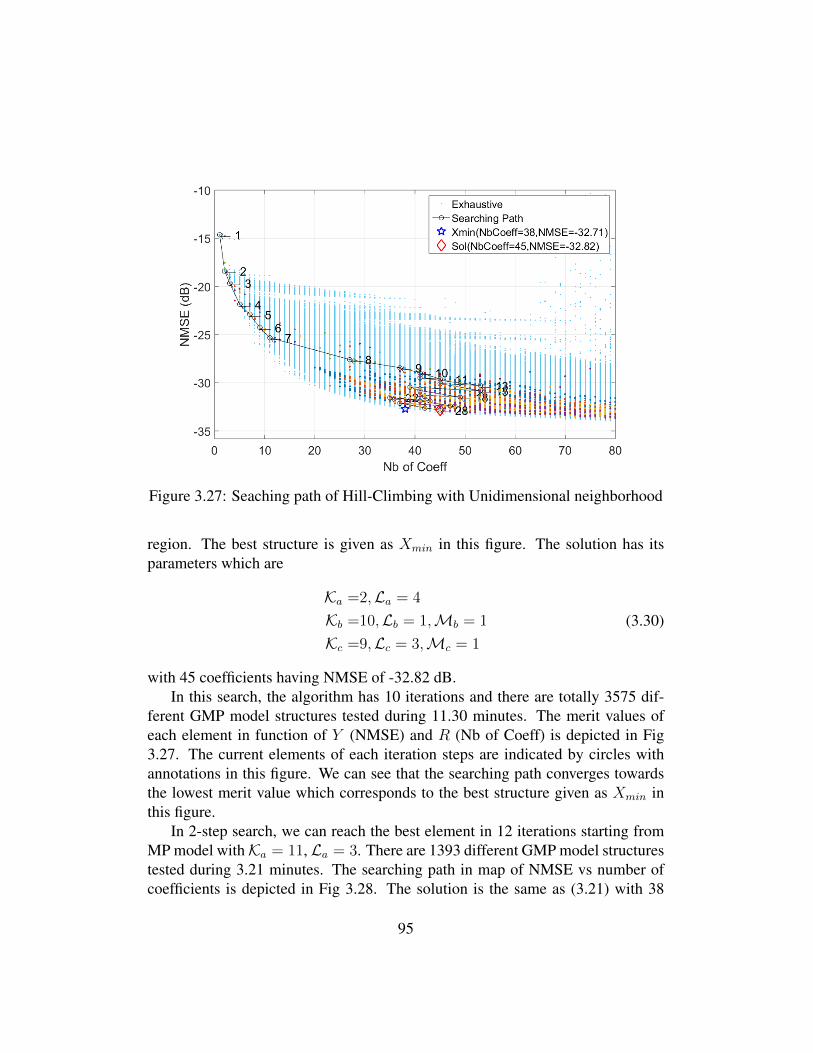
Figure 3.27: Seaching path of Hill-Climbing with Unidimensional neighborhood
region. The best structure is given as Xmin in this figure. The solution has itsparameters which are
Ka =2,La = 4
Kb =10,Lb = 1,Mb = 1
Kc =9,Lc = 3,Mc = 1
(3.30)
with 45 coefficients having NMSE of -32.82 dB.In this search, the algorithm has 10 iterations and there are totally 3575 dif-
ferent GMP model structures tested during 11.30 minutes. The merit values ofeach element in function of Y (NMSE) and R (Nb of Coeff) is depicted in Fig3.27. The current elements of each iteration steps are indicated by circles withannotations in this figure. We can see that the searching path converges towardsthe lowest merit value which corresponds to the best structure given as Xmin inthis figure.
In 2-step search, we can reach the best element in 12 iterations starting fromMP model withKa = 11, La = 3. There are 1393 different GMP model structurestested during 3.21 minutes. The searching path in map of NMSE vs number ofcoefficients is depicted in Fig 3.28. The solution is the same as (3.21) with 38
95
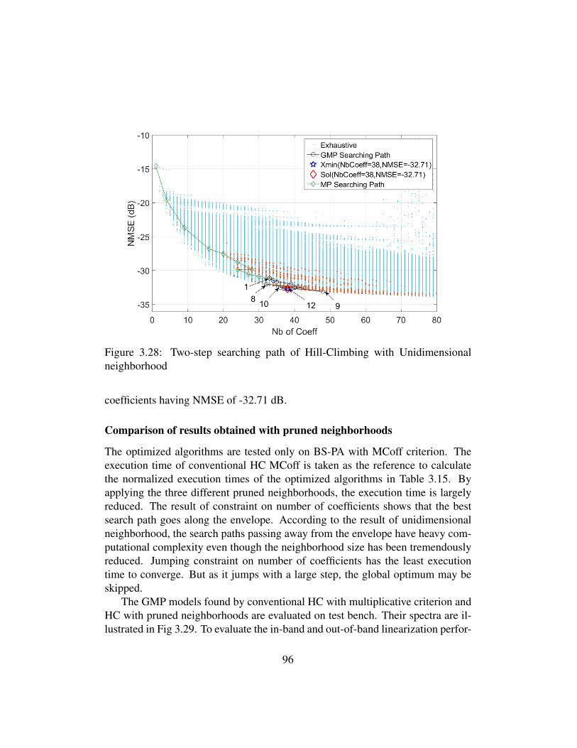
Figure 3.28: Two-step searching path of Hill-Climbing with Unidimensionalneighborhood
coefficients having NMSE of -32.71 dB.
Comparison of results obtained with pruned neighborhoods
The optimized algorithms are tested only on BS-PA with MCoff criterion. Theexecution time of conventional HC MCoff is taken as the reference to calculatethe normalized execution times of the optimized algorithms in Table 3.15. Byapplying the three different pruned neighborhoods, the execution time is largelyreduced. The result of constraint on number of coefficients shows that the bestsearch path goes along the envelope. According to the result of unidimensionalneighborhood, the search paths passing away from the envelope have heavy com-putational complexity even though the neighborhood size has been tremendouslyreduced. Jumping constraint on number of coefficients has the least executiontime to converge. But as it jumps with a large step, the global optimum may beskipped.
The GMP models found by conventional HC with multiplicative criterion andHC with pruned neighborhoods are evaluated on test bench. Their spectra are il-lustrated in Fig 3.29. To evaluate the in-band and out-of-band linearization perfor-
96

Table 3.15: Comparison of Search Results of HC with Different Optimizations onBS-PA
Conv( 2): Conventional algorithm using MCoff criterion(two-step)Optim1( 2): Constraint on NbCoeff is applied(two-step)Optim2( 2): Jumping constraint on NbCoeff is applied(two-step)Optim3( 2): Neighborhood is unidimensional(two-step)
Conv Optim1 Optim2 Optim3NMSEdB -32.71 -32.71 -32.65 -32.82NbCoeff 38 38 37 45Nb of Test 19598 3835 1438 3575Nb of Iter 11 21 18 10Ex. Time 1 0.16 0.08 0.38
Conv 2 Optim1 2 Optim2 2 Optim3 2NMSEdB -33.04 -32.71 -32.61 -32.71NbCoeff 44 38 38 38Nb of Test 39+7364 39+959 39+725 39+1393Nb of Iter 11+4 11+7 11+7 11+12Ex. Time 0.46 0.06 0.04 0.11
mances, error vector magnitude (EVM) and adjacent channel power ratio (ACPR)are listed in Table 3.16.
According to Fig 3.29 and Table 3.16, we can see that the linearization per-formances of the GMP models found by different means are close to each other.This confirms the efficiency of the proposed method in searching for the optimalGMP structures. And the proposed optimization methods do not deteriorate therobustness of the algorithm but tremendously improve the execution time.
All these optimizations are based on controlling the definition of the neigh-borhood during the search, which confirms the advantage of HC on the otheralgorithms with randomness.
97

Conv MCoff: Conventional HC with multiplicative criterion (3.21)Conv MCoff2: Conventional HC with multiplicative criterion in 2-step (3.22)Optim2: HC with jumping constraint on number of coefficients (3.28)Optim2 2: HC with jumping constraint on number of coefficients in 2-step (3.29)Optim3: HC with unidimensional neighborhood (3.30)
Figure 3.29: Comparison of spectra of Doherty PA output linearized by differentDPD
Table 3.16: Performance comparison of GMP model solutions
GMP GMP GMP GMP GMP(3.21) (3.22) (3.28) (3.29) (3.30)
Nb of Coeff 38 44 37 38 45EVM(%) 3.4 4.8 3.3 4.0 3.0ACPR L1 gain(dB) 18.4 18.3 17.8 18.9 18.5ACPR U1 gain(dB) 18.1 17.8 17.8 18.9 18.2
98

3.8 Comparison Between Genetic Algorithm and Hill-Climbing Heuristic
3.8.1 Integer Genetic algorithmA method using an integer genetic algorithm (GA) to select the orders of nonlin-earities and memory lengths of the GMP model has been proposed in [62].
Genetic algorithms are stochastic search mechanisms inspired by the processof natural evolution. It is based on the idea of Darwinian natural selection theorythat individuals with low values of quality will be eliminated and only those genesof good quality can be preserved in successive generations [78]. The quality ismodeled by a fitness function in GA. In our implementation, the fitness functionis given by the additive criterion (3.1).
To size the GMP model, the standard GA with functions for generating integerpopulation and integer mutations is used in [62]. A vector of integer numbersrepresents the structure of a GMP model. The applied GA algorithm is describedin Algorithm 3.
The initial population P individuals is generated as a random vector of integernumbers (Ka,Kb,Kc, La, Lb, Lc,Mb,Mc) which represents a chromosome madeof genes at the beginning of the algorithm. The fitness function of the individualxi(q) at the q-th generation is denoted by Ji(q). And Q is the maximum generationnumber that the algorithm can reach.
At each generation, the offspring is created in three ways: selection, crossoverand mutation. The groups of created offspring are denoted by O1, O2 and O3
respectively.
• Selection: The best 5% of P are kept in the next generation as offspring O1.
• Crossover: The parents can be represented in binary. For the parent Pi, itsbinary vector vi are subdividing into groups vi = [g1,i g2,i], and same forother parents. The crossover between Pi and Pj is to regroup g1,i, g2,i andg1,j , g1,j into new vectors, e.g. [g1,i g2,j] and [g2,j g1,j], etc.
• Mutation: The binary vectors can have some random variation on the bits.
The parents of the following generation is the sum of O1, O2 and O3.The Stall condition is that the number of iterations reaches the limit or the
fitness values variance of the population is lower than a threshold.
99

In this section, we compare the performances of these two methods for the siz-ing of GMP model structure using the same criterion based on trade-off betweenits modeling accuracy and complexity.
Algorithm 3: Overview of Genetic Algorithm
Set generation counter q = 1;Generate initial random integer populations of P individuals;while q 6 Q do
Compute fitness of all individuals;Selection: The best 5% of P are kept as offspring O1;Crossover: The 80% of the rest (P−O1) are subdivided into groupsand combined with each other to create offspring O2 ;
Mutation: for the rest, their genes in a chromosome are randomlychanged to create offspring O3;
q=q+1;P = O1 + O2 + O3;if Stall then
end while loop;end
end
3.8.2 Performance comparisonIn this section, we test only the additive criterion. If we choose µ = 0.065, thebest GMP model according to (3.1) has 38 coefficients (Ka = 11,La = 2,Kb =4,Lb = 1,Mb = 1,Kc = 3,Lc = 4,Mc = 1) and -32.71 dB NMSEdB.
The two algorithms (GA and HC) have pretty different behaviors. HC is adeterministic algorithm looking at each step for the neighbor which has a bettermerit function, it can therefore be sensitive to local extrema. On the other side theGA algorithm may be seen as a probabilistic search starting from random initialpopulation randomly spread throughout the whole solution space. Thus it couldbe quite sensitive to the size of the population which in turn has an impact on thecomplexity.
The sensitivity of the GA to different population sizes P is illustrated in Table3.17 while its sensitivity to the number of ”generation” (iteration) is highlightedby Table 3.18. By analyzing Table 3.17, we can see that the population size has
100

Table 3.17: GMP Results of Genetic Algorithm with Different Generation Sizes(µ = 0.065)
Population Size 50 100 150 200NMSEdB -32.22 -31.73 -32.71 -32.65NbCoeff 40 34 38 37Nb of Gen. 10 10 10 10Ex. Time 5.48 min 10.99 min 14.63 min 20.35 min
Table 3.18: GMP Results of Genetic Algorithm with Different Total Numbers ofGeneration (µ = 0.065)
Population Size 100 100 100 100NMSEdB -32.50 -32.74 -32.34 -32.48NbCoeff 37 42 36 35Nb of Gen. 15 20 25 30Ex. Time 13.72 min 17.81 min 19.80 min 22.52 min
a strong impact for the convergence towards the global optimum. We can checkthat the final solution is able to converge to the optimum when the population sizeis equal to or larger than 150 in this case. Table 3.18 shows that the increase ofthe number of generations does not help to converge towards the global optimumas the increase of the population size.
The results obtained with the HC algorithm and its convergence behavior aresummarized in the two left columns of Table 3.19 and in Fig 3.30. From thispicture we can see that HC behaves like a descent algorithm with iterations.
Table 3.19 allow to make some comparisons between both algorithms. Firstwe can check that HC is able to converge to the global optimum while GA con-verges to a solution very close to this optimum solution but with a slightly highercomplexity. The right column of Table 3.19 highlights that, unsurprisingly thetwo step approach does not improve the convergence speed and behavior of theGA algorithm, likely because of its randomness.
The lower subtable of Table 3.19 shows that different walks of the GA al-gorithms could lead to pretty different solutions. As the GA is a random searchprocedure, it may be improved by launching multiple times the GA search, pick-ing the best solution among the results. This will make its performance morestable, but this will increase the execution time.
101
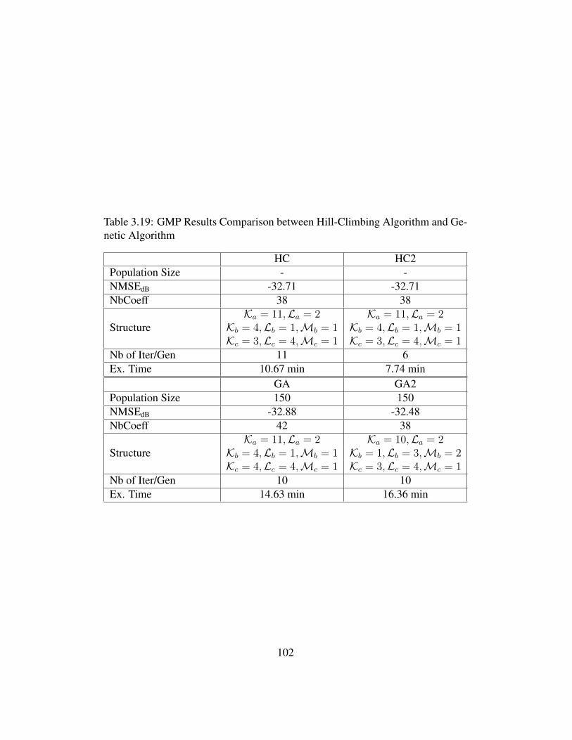
Table 3.19: GMP Results Comparison between Hill-Climbing Algorithm and Ge-netic Algorithm
HC HC2Population Size - -NMSEdB -32.71 -32.71NbCoeff 38 38
StructureKa = 11,La = 2 Ka = 11,La = 2
Kb = 4,Lb = 1,Mb = 1 Kb = 4,Lb = 1,Mb = 1Kc = 3,Lc = 4,Mc = 1 Kc = 3,Lc = 4,Mc = 1
Nb of Iter/Gen 11 6Ex. Time 10.67 min 7.74 min
GA GA2Population Size 150 150NMSEdB -32.88 -32.48NbCoeff 42 38
StructureKa = 11,La = 2 Ka = 10,La = 2
Kb = 4,Lb = 1,Mb = 1 Kb = 1,Lb = 3,Mb = 2Kc = 4,Lc = 4,Mc = 1 Kc = 3,Lc = 4,Mc = 1
Nb of Iter/Gen 10 10Ex. Time 14.63 min 16.36 min
102

Figure 3.30: Hill-Climbing heuristic searching path in function of NMSE andnumber of coefficients in 3D (µ = 0.065)
3.8.3 ConclusionGA is an algorithm strongly depending on user settings, e.g. population size andtotal number of generation. Large population size helps approaching the bestGMP result, but this also increases the execution time. With some appropriatesettings, GA and HC have very approximate performances which converge to theglobal optimum in a short time compared with exhaustive search.
The advantage of HC as well demonstrated in the previous sections is that wecan optimize the searching time by controlling the search path. But GA cannot becontrolled because of its randomness.
3.9 First-Choice Hill ClimbingFor the HC technique, we can also reduce the number of tested elements by con-trolling the search procedure among the neighbors, e.g. First-choice technique.
To reduce the number of tests during the search, we propose to test the neigh-bors under a certain condition, instead of testing all of them. The first testedneighbor which has better merit value than that of the current solution will betaken directly as the solution and the rest of neighborhood will not be tested. A
103

new iteration starts immediately. The neighbors are tested one by one followinga random order, e.g. uniform law. The search procedure terminates when there isno neighbor better than the current solution. Then this solution is the solution ofthe algorithm. In this procedure, we added randomness to the algorithm and thefinal solution will not be always the same for each search.
This optimization method differs from the formers as it changes the searchprocedure instead of the neighborhood definition. However the induced random-ness decreases its potential to be controlled and improved furthermore.
The light blue points in Fig 3.31 are all the possible GMP models in functionof Y (NMSEdB) and R (number of coefficients) in the search space. The colorfulpoints represents the models tested during the search.
Using HC with ACoff, 10821 models are tested during 15.9 minutes and thesolution is (3.21).
With FCHC, we have 16 iterations and totally 1691 structures of differentGMP models are tested. The solutions of each iteration are indicated by the circleson the search path as shown in Fig 3.31. The search path converges towards theoptimum Xmin. The solution found by the algorithm is
Ka =3,La = 2
Kb =4,Lb = 1,Mb = 1
Kc =10,Lc = 3,Mc = 1
(3.31)
with 40 coefficients and NMSEdB of −32.28 dB. The execution time is 4.2 min-utes.
As in this algorithm the neighbors are randomly chosen, We launch more timesto verify the stability of the algorithm. Fig 3.32 shows another search path whichalso converges towardsXmin. There are totally 4382 models tested in 15 iterationsduring 5.6 minutes. The final solution is
Ka =11,La = 2
Kb =1,Lb = 4,Mb = 1
Kc =3,Lc = 3,Mc = 1
(3.32)
with 35 coefficients and NMSEdB of −32.48 dB.We can see that the found solutions have different structures but their lineariza-
tion performances and execution times in search are very close.The structure of GMP models (3.31) and (3.32) are evaluated on PA. The spec-
tra of linearized PA output are illustrated in Fig 3.33. The blue curve is the spec-trum corresponding to model 3.31 and the red curve is the spectrum corresponding
104

Figure 3.31: Result 1 of FCHC search
Figure 3.32: Result 2 of FCHC search
105

Figure 3.33: Comparison of spectra of Doherty PA output linearized by differentDPD
to model 3.32. Their performances are very similar. The green curve is the spec-trum of the reference GMP model (3.21).
To evaluate the in-band and out-of-band linearization performances, error vec-tor magnitude (EVM) and adjacent channel power ratio (ACPR) are listed inTab 3.20. The stability of FCHC is confirmed by the similarity of the perfor-mances of these two models.
We can see that the execution time of First-choice hill-climbing is only onethird of that of conventional HC.
3.10 ConclusionIn this chapter, an algorithm is presented to find the optimal GMP model struc-ture with a very limited number of computations. Two search criteria performinga trade-off between complexity and modeling accuracy of the GMP model arecompared.
The algorithm is applied on two different dataset: signals of Base station PAand signals of broadcast PA. The characteristics of these two PAs and their inputsignals are very different. The performances of the proposed algorithm are good
106

Table 3.20: Performance comparison of GMP models obtained with FCHC
GMP (3.21) GMP 1 GMP 2Nb of Coeff 38 40 35EVM(%) 2.3 3.2 2.6ACPR L1 gain(dB) 19.3 18.8 19.0ACPR U1 gain(dB) 19.1 18.8 18.3Ex. Time 15.9 min 4.2 min 5.6 min
in both cases, which confirm the robustness of the algorithm.Several optimizations of the algorithm are proposed and verified. The opti-
mizations are made by giving different constraints on the neighborhood of searchor on the search procedure. The results show that the computational complexityof search is dependent on the search path. When the search path follows the enve-lope edge of exhaustive result cloud, the complexity is lower compared with thecase that search path is far from the envelope.
A comparison between hill-climbing and genetic algorithm is made. They mayhave similar performances when the parameters of algorithms are well configured.
The genetic algorithm relies more on the population size which has a greatimpact on convergence speed and computational complexity. One of the advan-tages of the hill-climbing algorithm compared with evolutionary algorithms is thatthe search path can be controlled by configuring the parameters, which results indifferent optimizations on execution time.
The technique to determine the optimal single-block DPD is proved robust inthis Chapter and will be applied in case of cascaded DPD in the next chapter.
107

Chapter 4
Multi-stage Cascaded DigitalPredistortion
4.1 IntroductionPD model can be not only one system, but also an union of several systems.Cascaded DPDs are found beneficial by some researches in [79], [3], [80], [81].In [79], the cascaded model is identified in a nonparametric method. A paramet-ric identification using multi-stage ILA is proposed in [3]. In [80], a two-stageDPD is used to compensate separately for high-order memoryless nonlinearitiesand low-order memory effects. The nonlinear bloc is realized with a look-up table(LUT) which is identified using ILA. The memory bloc is upstream of the nonlin-ear bloc, which is identified using DLA. In [81], a three-layer DPD is proposed asa bias information is introduced in the second layer.
Hammerstein, Wiener, and Wiener-Hammerstein models are widely used andtheir identification algorithms are thoroughly researched [82] [83]. In [82], theWiener model is identified using particle swarm optimization (PSO) instead ofleast squares (LS). An enhanced Hammerstein model is proposed in [83] to sup-press the spectrum regrowth caused by the memory effects. A branch parallel tothe linear filter bloc is added where the input signal is multiplied by its magnitude.Each stage of the cascaded model is identified separately at different iterations.
Different multi-stage cascaded models have been studied in recent years, suchas multi-stage Volterra Series [84], multi-stage MP models [85] or multi-stageGMP models [86].
The advantage of cascaded-structure PD is the relative simplicity of the low
108

order modules in terms of computational complexity and extensibility to the re-alization of higher-order functions [87]. Though the identification of cascadedDPD needs additional steps, the complexity increase of the identification task canbe compensated for by the lower number of model coefficients [88].
This chapter is organized as follows. Block-oriented Nonlinear System iden-tification methods are presented in Section 2. Identification methods of generalmulti-stage cascaded DPD are presented in Section 3. Section 4 gives some cas-caded DPD performances experimental studies and analysis. An algorithm andcriterion is used in Section 5 to find the optimal structure of cascaded DPD model.Section 6 gives a brief conclusion.
4.2 Block-oriented Nonlinear System IdentificationIdentification of multi-stage cascaded DPD is more complicated than that of single-stage model. A particular case of multi-stage cascaded DPD is the block-orientednonlinear (BONL) system. The BONL structure is composed of blocks connectedin series or in parallel: the Hammerstein model as Fig 2.9 and the Wiener model asFig 2.10 are particular cases. The identification of Wiener or Hammerstein modelhas been studied in [89] [90] [91] [92].
The iterative identification algorithm of Hammerstein model proposed by Naren-dra and Gallman in [89] has been used in [93] for DPD. The Hammerstein modelin Fig 2.9 which can be described by (2.21) and (2.22) is identified by an itera-tive method alternately adjusting the coefficients ak and bl by least square (LS)method. In this algorithm, a relationship among the coefficients of nonlinear part,memory effect part and passing signals is built. First of all, we need to initializethe values of ak. By knowing the coefficients of nonlinear part, we can calculatethe coefficients of memory effect part, and vice versa. In the following iterations,we can calculate the coefficients of both two parts iteratively till the algorithmconverges.
A non-iterative method for Hammerstein identification was proposed in [90].In this method, the values of ck,l =
∑K−1k=1
∑L−1l=0 akbl are estimated in one iteration
with the input and output signals of the system. Here a0 is assumed unity andother coefficients ak (k > 0) are normalized by a0. For each memory depth l(l ∈ [0;L− 1]), we can calculate a corresponding value of ak(l) by:
ak(l) =ck,lc0,l
(4.1)
109

where k ∈ [1;K−1]. If we denote the vector of coefficients by a = [a1, .., aK−1],there are L different possible coefficient vectors a(i) (i ∈ [0;L−1]). Each of themis tested and the one which generates the least error between the expected signaland measured signal is taken as the best. Comparing with iterative method, thismethod can reduce the computational complexity by limiting the iteration numberto only one, but the matrix size is largely increased (the array ck,l has K × Lelements where ak and bl have only K and L elements respectively). Thus thenon-iterative method has advantage only when the orders of model structure Kand L are lower than a certain threshold.
A discrete-time Hammerstein model is identified in [94]. The linear dynamicstage can be identified by the correlation between the input and output signals.Then the nonlinear stage is identified using kernel regression estimates which wasproposed independently by Nadaraya [95] and Watson [96]. With the same algo-rithm, the Wiener model is identified in a nonparametric method in [97].
Both iterative method and the correlation-based method have been two moststudied method for years. However, the convergence of iteration method is con-firmed in [91] and it is preferable because the correlation-based method with fi-nite data lengths can not cover any particular realization of the input process overa finite time period. The convergence of iterative identification of Hammersteinmodel is also confirmed in [98].
The identification of a Hammerstein-Wiener model (as Fig 2.12a) using max-imum likelihood (ML) estimation is discussed in [92]. The parameters vector ofthe system are denoted by θ = [aT , bT , cT ]T where a and c are coefficient vec-tors of nonlinear blocs and b is the coefficient vector of the middle linear filter.An estimate of θ is
θ = argmaxθLθ(YN) (4.2)
where YN are the measured output signal of the system, N is the number of real-izations. According to Bayes’ rule, the likelihood can be written as
Lθ(YN) =N∑t=1
log pθ(yt|Yt−1), pθ(y1|Y0) = pθ(y1) (4.3)
where yN are the estimated system output, pθ(y1) denotes the joint density of y1,and pθ(yt|Yt−1) is the prediction density for the realization Yt−1.
The initial values of the parameters are very important for the convergenceof ML to the global optimum. The best linear approximation (BLA) [99] and
110

Stage 2 Stage 1
MP MPu(n) x(n)w(n)
Figure 4.1: 2-stage MP model
ε-approximation [100] can be used to extract the simple function of the lineardynamic bloc in the system. In [36], BLA is applied to identify different types ofBONL with input signal u(t) and output signal y(t):
Gbla(ejωTs) =
SY U(ejωTs)
SUU(ejωTs)(4.4)
where SY U is the cross-power spectrum of y(t) and u(t), SUU is the auto-powerspectrum of u(t).
4.3 Identification of General Multi-stage DPD ModelFor general multi-stage cascaded DPD models, we identify stage by stage as pro-posed in [3]. As multi-stage DPD is composed of several cascaded blocks, theblock nearest to the PA is denoted by “Stage 1”. We take a 2-stage MP model asan example in this dissertation (Fig 4.1).
The relation between the input and output of DPD can be expressed as:
w(n) =
K2−1∑k=0
L2−1∑l=0
eklu(n− l)|u(n− l)|k
x(n) =
K1−1∑k=0
L1−1∑l=0
hklw(n− l)|w(n− l)|k(4.5)
where u(n) and x(n) are the input and output signal of the DPD respectively,w(n)is the output signal of Stage 2.
In case of a 2-stage MP as (4.5), we can model a DPD which has nonlinearitiesof order K1K2 and memory depth of order L1 + L2 − 2. The total number ofcoefficients is K1L1 + K2L2. But the values of the coefficients have very strongconstraints. The coefficients of the equivalent predistorter structure comes fromthe product combinations of the coefficients of the 2 stages MP models.
The identification procedure using indirect learning structure (ILA) of cas-caded DPD is presented in this section (Fig 4.2). A Post-inverse of each stage is
111

estimation
Parametersestimation
Parameters
parametersCopying
PA2 1
Stage Stage
1
Post−inverse
2
Post−inverse
Pre−inverse: PD
zp2(n)
x2(n)u(n) x1(n) y(n)
z(n)
ε2(n) = zp2(n)− x2(n)ε1(n) = zp1(n)− x1(n) ε2(n)
ε1(n)
zp1(n)
1G
Figure 4.2: Indirect Learning Architecture - ILA
identified and used in the Pre-inverse block as a DPD. The identifications of bothstages have the same procedure. Thus we take Stage 2 as an example.
The total number of coefficients of Stage 2 is R2 = K2L2. For a total numberof samples equal to N , we can write
zp2 = Za (4.6)
where zp2= [zp2(1), . . . , zp2(N)]T is the vector of output samples of the post-inverse, Z is a N ×R matrix of basis functions of z, a is the vector of coefficientsakl. The Least square (LS) solution of (4.6) is also the solution of the normalequation
[ZHZ]a = ZHx2 (4.7)
where a is the estimated value of a.For the identification of multi-stage DPD, all stages can be identified with ILA
iteratively in two ways: the order of identification from the stage furthest from thePA to the stage closest to the PA is called “forward (FW)”; (Fig 4.3a) the order ofidentification from the stage closest to the PA to the stage furthest from the PA iscalled “backward (BW)”. (Fig 4.3b) The DPD stages are identified in an alternateway: after the last stage is identified, the following system iteration restarts fromstage 1. We can re-identify the other stages after the modification of one stage.
In each system iteration, only one stage of DPD is identified while other stagesare applied [3].
112

3 2 1
2 3
3 2 1
3
2 1
3
3
11
1
2Forward Forward
Forward
(a) Forward (FW) order
2 1 3 2 1
2 32 3
3 2 1
3
1
3
Backward
Backward
Backward
(b) Backward (BW) order
Figure 4.3: Identification order of multi-stage DPD
4.4 Experimental Results for Multi-stage MP modelDPD
4.4.1 Case of a cascade of 2 low order MP modelsIn the following experiments, each stage is identified with 4 iterations. The DPDidentification dataset buffer size is 6 000 samples. The DPD performance is eval-uated on BS-PA with an LTE signal of 240 000 samples.
The simplest cascaded DPD is composed of only two stages. We choose thefollowing cascaded MP structures:Model K6L2/K2L6
K1 =6, L1 = 2
K2 =2, L2 = 6(4.8)
and Model K2L6/K6L2
K1 =2, L1 = 6
K2 =6, L2 = 2.(4.9)
Both of them have 24 coefficients.
113

The computational complexity depends on the number of samples N and onthe total number of coefficients of the model. The main computation load comesfrom finding the solution of (4.7). We consider solving (4.7) using a QR decom-position. If N is large compared to R, we can estimate the computation load byO(2NR2). As 2N is a constant, we express the complexity with R2. The com-plexities of (4.9) and (4.8) are both 288.
In purpose of reference, we choose three MP models of similar complexity totest:Model K6L4
K = 6, L = 4; (4.10)
which has 24 coefficients with complexity equal to 576.Model K6L3
K = 6, L = 3; (4.11)
which has 18 coefficients with complexity equal to 324.Model K5L3
K = 5, L = 3. (4.12)
which has 15 coefficients with complexity equal to 225.The model K6L4 is chosen because it has the same number of coefficients
with the proposed cascaded MP model. The model K6L3 is chosen because it issimilar to one stage of the proposed cascaded MP model and it has also a veryclose complexity to the proposed cascaded MP model. The model K5L3 is cho-sen because a model with complexity less than the proposed cascaded MP modelneeds to be tested as a reference.
The spectra of output signal of PA linearized with MP DPD (4.10)-(4.12) areshown in Fig 4.4. We can see that Model K6L4 has better linearization perfor-mance and it is taken as a reference in Fig 4.7 to compare with the cascaded MPmodels.
The spectra of output signal of PA linearized with Model K6L2/K2L6 in dif-ferent identification orders are shown in Fig 4.5. The light blue curve is the outputof PA without DPD. The linearization performance of BW is better than that ofFW. The spectra of output signal of PA linearized with Model K2L6/K6L2 in dif-ferent identification orders are shown in Fig 4.6. In this case, the linearizationperformance of FW is better than that of BW.
114

Figure 4.4: Spectra of Doherty PA output linearized by different MP DPD
In Fig 4.7, we compare the best results that the MP model and two cascadedmodels can achieve. We can see that Model K6L2/K2L6 and Model K2L6/K6L2have the same performance and both of them outperform Model K6L4. This isconfirmed in Table 4.1. In this table, the error vector magnitude (EVM) of theoutput signal and the first-adjacent-channel adjacent channel power ratio (ACPR)gain of the DPD identified with different algorithms are used to evaluate the lin-earization performances. The ACPR gain is the improvement of ACPR after lin-earization compared with the the output of PA without DPD.
Each stage of Model K6L2/K2L6 or Model K2L6/K6L2 have the same dimen-sion, but one stage represents mainly nonlinearity and the other one representsmainly memory effect. Fig 4.5 and Fig 4.6 show that the identification of DPDstarting from the model with the higher nonlinearity can always achieve the bestperformance of a given model. Fig 4.7 shows that cascaded DPDs with differentstructures can reach the same performance, which confirms that linearization per-formance of cascaded DPD depends not on the order of the blocks in the cascade.
Conclusion
In this section, we analyzed the interest of using a 2-stage cascaded DPD com-posed of two different low order MP models. By switching the order of the
115

Figure 4.5: Spectra of Doherty PA output linearized by Model K6L2/K2L6 withdifferent identification
Figure 4.6: Spectra of Doherty PA output linearized by Model K2L6/K6L2 withdifferent identification
116

Figure 4.7: Comparison of spectra of Doherty PA output linearized by differentDPD
Table 4.1: Performance comparison of 3 DPD models
ACPR L1 ACPR U1 EVM J2
gain (dB) gain (dB) (%)K6L4 14.3 11.8 5.2 576K6L3 13.2 10.1 6.8 324K5L3 13.0 10.1 6.7 225K6L2/K2L6 FW 9.7 8.7 9.7 288K6L2/K2L6 BW 14.9 12.9 5.8 288K2L6/K6L2 FW 14.2 12.4 5.3 288K2L6/K6L2 BW 12.6 12.1 8.3 288
117

two stages, we compared their performances. We showed that the identificationmethod of 2-stage cascaded DPD is of importance and the stage with higher non-linearity order should be identified first. In the test case here, the switching of thestages does not alter the linearization performance provided that the right identi-fication procedure is conducted.
4.4.2 Comparison of a multi-stage cascaded MP DPD with asingle-stage MP or GMP model
This section makes an experimental study on comparison between a single-stageDPD and a multi-stage cascaded DPD model. The performance of cascaded DPDmodel is evaluated with the Three-way Doherty PA (BS-PA) and LTE signal.
To make a comparison between the single stage DPD and multi-stage DPD,we tested an MP model, a GMP model and a 2-stage MP model which have verysimilar number of coefficients.
Using our hill-climbing method, we can find an appropriate GMP model struc-ture:
Kb =11, Lb = 2
Kc =1, Lc = 3,Mc = 3
Kd =3, Ld = 4,Md = 1.
(4.13)
As the GMP model has totally 43 coefficients, the MP model structure is setas
K =11, L = 4. (4.14)
The 2-stage MP structure is arbitrarily set as:
K1 =9, L1 = 4
K2 =4, L2 = 2.(4.15)
In the following experiments, each stage is identified with 4 iterations. For ex-ample in case of BW, firstly we identify the stage 1 for 4 iterations. Then we fixthe stage 1 and identify the stage 2 for 4 iterations. This procedure is denoted by“system iteration”. In this section, the cascaded DPDs are identified with 2 systemiterations.
The results of 8th iteration are shown in Fig 4.8 and Table 4.3. The DPD iden-tification dataset buffer size is 6 000 samples. The DPD performance is evaluatedwith an LTE signal of 240 000 samples.
118

Table 4.2: Performance comparison of 3 DPD models
GMP MP 2-stage MPEVM(%) 2.34 5.86 3.66ACPR L1 gain(dB) 19.1 16.1 17.1ACPR U1 gain(dB) 18.1 15.3 16.0
The spectra of output signal of linearized PA are shown in Fig 4.8. The lightblue curve is the output of PA without DPD. The red, green and black curves arethe output of PA with DPD of 2-stage MP model, MP model and GMP modelrespectively.
These three DPDs have very close linearization performances. The GMPmodel DPD can reach the best linearization performance. Comparing with MPmodel, the performance of 2-stage MP is a little better.
Table 4.2 shows the EVM of the output signal and the first-adjacent-channelACPR gain of the DPD identified with different algorithms compared with theoutput of PA without DPD while applying each model. We can see that 2-stageMP has the best in-band performance and the out-band performance is betweenthe MP model and GMP model.
Table 4.3 shows the number of coefficients of each model, the dynamic rangeof model coefficients (the difference between the maximum and the minimum),the condition number of the matrix computation in identification procedure andthe normalized complexity (Number of complex multiplications normalized bythat of the MP case). The dynamic ranges of coefficients of GMP and MP mod-els are large and their matrices exhibit large condition numbers. For “2-stageMP” model, the number of coefficients, EVM and ACPR are close to GMP andMP models, but its computational complexity is much less. As “2-stage MP”model has less order in nonlinearity and memory depth in each stage, its condi-tion number is smaller by a factor of 100. The complexity of “2-stage MP” modelidentification is also reduced by more than 30%.
In this section, we analyzed the interest of using a multi-stage cascaded digitalpredistorter composed of two MP models. We compared its performance with thatof a single stage predistorter made of an MP or GMP model. The optimal structure(orders of non-linearity and memory lengths) of the single stage DPD (MP orGMP) are determined using an HC, but the 2-stage MP model is determined in anad-hoc way. GMP model reaches the best linearization performance but using a
119

Figure 4.8: Comparison of spectra of Doherty PA output linearized by differentDPD
Table 4.3: Performance comparison of 3 DPD models
GMP MP 2-stage MPStage 1 Stage 2
Number of Coefficients 43 44 36 8Coeff Dynamic Range 4.0e6 4.7e6 4.2e5 7.4Condition Number 8.8e18 1.1e19 7.6e16 3.0e6
Normalized Complexity 0.96 1 0.67 0.04
120

2-stage MP model can decrease the complexity and dynamic range of coefficientsand improve the condition number of the identification of the DPD parameters.
In this comparison, we have chosen arbitrarily the structure of the 2-stageDPD. In the next section, we propose a method to size the cascaded DPD structure.
4.5 Sizing of Cascade DPD StructureIn this section we apply the method proposed in Chapter 3 to size a cascadedmodel. We propose a new criterion to represent the trade-off between modelingaccuracy and the complexity of model identification. A 2-stage MP model ischosen to be the cascaded DPD in this section. Its performance is evaluated witha Three-way Doherty PA.
4.5.1 Search Algorithm and CriterionIn a discrete set, each node xi is assigned to a unique cascaded MP model struc-ture. The coordinate of xi consists of 4 dimensions: K(i)
1 , L(i)1 , K(i)
2 , L(i)2 . The
value of a merit function J(xi) is associated to each node xi.The searching procedure is described in Algorithm 1.In our implementation, we define a neighbor of node xi as a node of which
parameters are K(i)1 + δ1, L(i)
1 + δ2, K(i)2 + δ3, L(i)
2 + δ4, where δ1,...,4 ∈ [0,±1] andδ1,...,4 are not 0 at the same time.
The merit value of the node xi here refers to a criterion Ji which leads to atradeoff between modeling accuracy and model complexity. NMSE value (2.7)denoted by Y , is the criterion to judge the modeling accuracy. The complexity ofmodel identification is represented by the square sum of number of coefficients ofthe model which is denoted by R2
1 +R22.
We combine the objective on the number of coefficient and the constraint onthe NMSE in a single criterion, using a trade-off weight coefficient λ:
Ji = Yi + λ(R21,i +R2
2,i). (4.16)
4.5.2 Experimental ValidationIn this section we evaluate our algorithm with 2 values of λ corresponding to twotrade-offs between the modeling accuracy and complexity of models identifica-tion. The values used for λ are: 1e−3 and 2e−3.
121
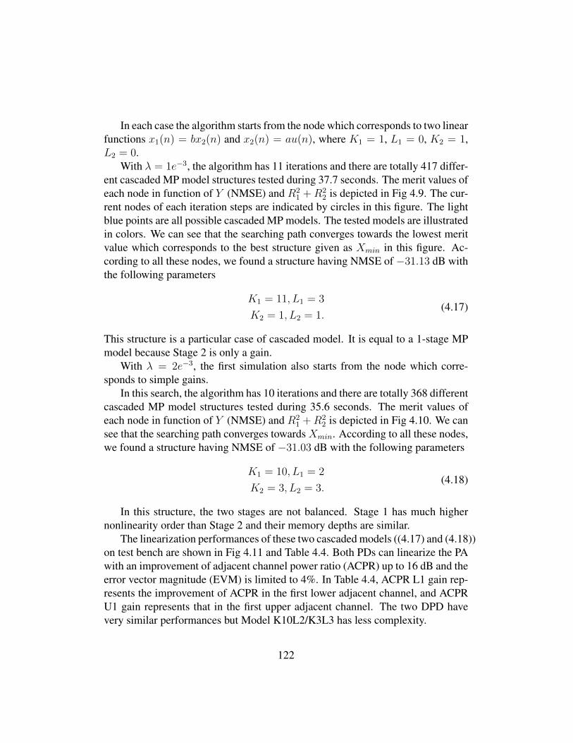
In each case the algorithm starts from the node which corresponds to two linearfunctions x1(n) = bx2(n) and x2(n) = au(n), where K1 = 1, L1 = 0, K2 = 1,L2 = 0.
With λ = 1e−3, the algorithm has 11 iterations and there are totally 417 differ-ent cascaded MP model structures tested during 37.7 seconds. The merit values ofeach node in function of Y (NMSE) and R2
1 +R22 is depicted in Fig 4.9. The cur-
rent nodes of each iteration steps are indicated by circles in this figure. The lightblue points are all possible cascaded MP models. The tested models are illustratedin colors. We can see that the searching path converges towards the lowest meritvalue which corresponds to the best structure given as Xmin in this figure. Ac-cording to all these nodes, we found a structure having NMSE of −31.13 dB withthe following parameters
K1 = 11, L1 = 3
K2 = 1, L2 = 1.(4.17)
This structure is a particular case of cascaded model. It is equal to a 1-stage MPmodel because Stage 2 is only a gain.
With λ = 2e−3, the first simulation also starts from the node which corre-sponds to simple gains.
In this search, the algorithm has 10 iterations and there are totally 368 differentcascaded MP model structures tested during 35.6 seconds. The merit values ofeach node in function of Y (NMSE) and R2
1 +R22 is depicted in Fig 4.10. We can
see that the searching path converges towards Xmin. According to all these nodes,we found a structure having NMSE of −31.03 dB with the following parameters
K1 = 10, L1 = 2
K2 = 3, L2 = 3.(4.18)
In this structure, the two stages are not balanced. Stage 1 has much highernonlinearity order than Stage 2 and their memory depths are similar.
The linearization performances of these two cascaded models ((4.17) and (4.18))on test bench are shown in Fig 4.11 and Table 4.4. Both PDs can linearize the PAwith an improvement of adjacent channel power ratio (ACPR) up to 16 dB and theerror vector magnitude (EVM) is limited to 4%. In Table 4.4, ACPR L1 gain rep-resents the improvement of ACPR in the first lower adjacent channel, and ACPRU1 gain represents that in the first upper adjacent channel. The two DPD havevery similar performances but Model K10L2/K3L3 has less complexity.
122

Figure 4.9: Cascaded model structure searching path with λ equal to 1e−3
Figure 4.10: Cascaded model structure searching path with λ equal to 2e−3
123

Figure 4.11: Comparison of spectra of Doherty PA output linearized by foundDPD
Table 4.4: Performance comparison of 3 DPD models
ACPR L1 ACPR U1 EVM R21 +R2
2
gain (dB) gain (dB) (%)K11L3/K1L1 17.4 16.1 4.0 1090K10L2/K3L3 16.5 16.9 4.0 481
124
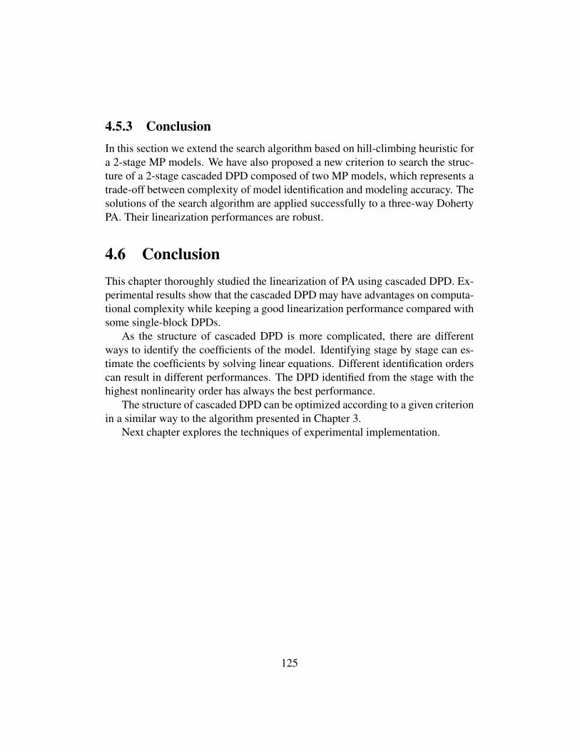
4.5.3 ConclusionIn this section we extend the search algorithm based on hill-climbing heuristic fora 2-stage MP models. We have also proposed a new criterion to search the struc-ture of a 2-stage cascaded DPD composed of two MP models, which represents atrade-off between complexity of model identification and modeling accuracy. Thesolutions of the search algorithm are applied successfully to a three-way DohertyPA. Their linearization performances are robust.
4.6 ConclusionThis chapter thoroughly studied the linearization of PA using cascaded DPD. Ex-perimental results show that the cascaded DPD may have advantages on computa-tional complexity while keeping a good linearization performance compared withsome single-block DPDs.
As the structure of cascaded DPD is more complicated, there are differentways to identify the coefficients of the model. Identifying stage by stage can es-timate the coefficients by solving linear equations. Different identification orderscan result in different performances. The DPD identified from the stage with thehighest nonlinearity order has always the best performance.
The structure of cascaded DPD can be optimized according to a given criterionin a similar way to the algorithm presented in Chapter 3.
Next chapter explores the techniques of experimental implementation.
125

Chapter 5
Impact of PA Gain Choices
5.1 IntroductionThe choice of the reference gain G used in predistortion has been discussed indifferent papers [101] [102] [103] [104].
The linearized PA gain which impacts the DPD model can be decided arbitrar-ily [101]. In particular, two very often used gains are the small signal gain G1 andthe peak power gain G2. The small signal gain G1 is the gain of the PA when itsbehavior is generally linear. The peak power gain G2 is calculated with the inputpeak power and output peak power of PA.
In [102], different normalization gains with look-up table (LUT) model DPDare tested. Zhu et al. [103] emphasize that usingG1 needs an extra calibration stepand using G2 does not. In [105], different normalization gains with memory poly-nomial (MP) model DPD are tested. The power alignment issue has been studiedand the normalization gain for which the average powers at the input and outputof the DPD is equal is considered optimal in [88]. In [106], G1 is applied and thegain of DPD is set unity. A one-step method to extract the optimal normalizationgain is proposed in [104]. The impact of choice of gains on the average outputpower of PA is studied in [107]. However, the scaling of gain is seldom discussedin terms of power added efficiency (PAE) in publications.
This chapter presents an experimental study of linearization and PAE with aThree-way Doherty PA at different choices of normalization gain. In Section 2,the power variation and PAE at the operating point are studied. And we propose anadjustment in the DPD identification to improve the PA linearization performancein case ofG1. The experimental results are presented in Section 3. Section 4 gives
126
Figure 5.1: PA input signal vs PA output signal
a brief conclusion.
5.2 Linearization of PA at different gains
5.2.1 PA power compression effectFrom Fig 2.14 we can see that: at the first iteration of identification, the PA inputsignal is x(n) = u(n), and the post-inverse block is estimated with signal z(n)which is the normalized output signal of PA; and at the second iteration, the esti-mated model of post-inverse block is applied at the pre-inverse block as the DPDwhile the DPD input signal is u(n).
Because of the nonlinearity of PA near to the saturation zone as shown inFig 5.1, the PAPR of PA output signal is compressed compared with the PAPR ofPA input signal. We can easily have PAPRu > PAPRz. Thus the input signalsof pre-inverse and post-inverse blocks are different.
As the signal z(n) is normalized by the gain G (z(n) = y(n)/G), the averagepower or peak power of z(n) can be decided by G. If we respect the consistency
127

Figure 5.2: Two choices of gain
of average power, so we should have
E(Pu) =E(Py)
G. (5.1)
If we respect the consistency of peak power, so we should have
max(Pu) =max(Py)
G. (5.2)
Howerver, the consistencies of average power and peak power cannot be respectedat the same time. We can also have different other choices of gain that none ofthem is respected.
In this dissertation, we choose only two gains as shown in Fig 5.2 to compare:small signal gainG1 and peak power gainG2. The output amplitude is normalizedby the chosen gain G1.
5.2.2 Linearization at G1
There are many different ways to set the normalization gain which is used tocalculate the coefficients of the DPD.
128

Figure 5.3: Small signal gain G1
The small signal gain G1 is calculated using the low amplitude input signals.We can make an approximation E(Pu) ≈ E(Pz).
In Fig 5.3, the blue curve shows the AM/AM curve of PA, and the green curveis the AM/AM curve of DPD identified with input and output signals of PA. Thepink line shows that the PA is linearized by the DPD. We can see that the outputsignal is saturated when the input signal amplitude is higher than a threshold.PPAOutSat is the saturated output of PA normalized by G1.
Therefore, we need to apply an input peak back-off (IPBO) to reduce the dy-namic range of the input signal. If we denote the threshold amplitude of the sys-tem input signal by Pth, a first step (calibration step) with a high power signalis needed to find out Pth. As PPAOutSat is the normalized PA saturated outputamplitude, the input saturation power Pth is obtained by
Pth = PPAOutSat. (5.3)
In this linearization method, the average power of the system input signal iskept at a constant value. In each iteration, the training signal z(n) has peak powerequals to E(Pu) + PAPRz. In the following iterations, this DPD model is fedwith a signal which has peak power equals to Pth = E(Pu) + PAPRu. AsPAPRu > PAPRz, the DPD model does not cover the entire power range of theinput signal. An extrapolation of the DPD characteristic function is needed for
129

(a) Iteration 1: Identification withoutBack-off
(b) Iteration 2: Identification with Back-off
Figure 5.4: Adjustment for small signal gain G1
the signals which have higher power than E(Pu) + PAPRz. This degrades theperformance of PA linearization.
5.2.3 Adjustment at G1
As discussed in the previous subsection, when G1 is chosen, the performance ofthe first identified DPD is degraded due to the extrapolation. The effect is evidentwhen the PA has very strong nonlinearity. We propose an adjustment as shown inFig 5.4:
• at the first iteration, a post-inverse model “M1”is identified without IPBO;
• at the second iteration, IPBO is applied on the input signal and “M1” isapplied as DPD, and a new post-inverse model “M2” is identified.
The peak power of training signal of “M1” is the input peak power beforeIPBO. If we take this signal to train the post-inverse model, the input power rangewill be covered.
Then at the second iteration, the output signal of DPD will not diverge and themodel “M2” can be identified.
130

Figure 5.5: Peak power gain G2
5.2.4 Linearization at G2
In case of peak power gain G2, the input power of PA should be high enough topush the PA to the critical point where it starts to be saturated. In Fig 5.5, the greenstraight line shows G2 of the PA linearized by DPD which is calculated with themaximal amplitude of signals at input and output of PA:
GPeak =PyPu. (5.4)
The advantage of this choice of gain is that no IPBO is needed and u(n) andz(n) have the same peak power. The drawback of this linearization method is thatthere is an average power difference between u(n) and z(n).
We can observe in Fig 5.5 that the average input power of DPD is higher thanthat of PA. In another word, the DPD compresses the power.
5.3 Experimental validationThe linearization performances are evaluated by the error vector magnitude (EVM)and the adjacent channel power ratio (ACPR) between the input signal of DPD andoutput signal of PA. The ACPR gain (ACPR G) is the improvement of ACPR ofPA output after applying DPD compared with the ACPR of PA output without
131

DPD. The EVM is not the real EVM as (2.9). Since we process the signals inbaseband, it is simply calculated by
EVM% =std(z(n)− u(n))
std(u(n))× 100% (5.5)
where u(n) is the stimulus signal, z(n) is the normalized PA output signal, std(·)calculates the standard deviation.
Using the method proposed in Chapter 3, we can find an appropriate GMPmodel structure:
Ka =11,La = 2
Kb =1,Lb = 3,Mb = 3
Kc =3,Lc = 4,Mc = 1.
(5.6)
5.3.1 Performance of linearization with adjustment at G1
The measured spectra at the output of the linearized PA are presented in Fig 5.6.The green curve represents the spectrum of PA output signal without DPD. Theblue curve shows the output signal spectrum of PA linearized at G1. The red andthe black curves are spectra of the output signal of linearized PA with the DPDidentified during the calibration step and during the second step respectively. Thespectra captured by FSW have 30 dB attenuation compared with the PA outputpower.
The measured ACPR gain and EVM are shown in Table 5.1. In the table, L1refers to lower band 1st adjacent channel, U1 refers to upper band 1st adjacentchannel, L2 refers to Lower band 2nd adjacent channel, U2 refers to Upper band2nd adjacent channel.
We can see that the adjusted method improves the ACPR gain of the lowerband 1st adjacent channel 9.52 dB, and the EVM is lowered from 15.3% to 6.2%.
Comparing these three spectra, we can see that the linearization with the ad-justment outperforms the method without adjustment on the linearization of PAboth in-band and out-of-band.
132

Table 5.1: Linearization performances of the PA at G1
Original AdjustedApproach 1st step 2nd step
ACPR Gain(G) (dB)
L1 6.17 9.35 15.69U1 4.99 12.84 15.69L2 0.98 5.81 9.02U2 -2.95 4.61 6.75
EVM (%) 13.3 23.2 4.2
Figure 5.6: Measured spectra of the linearized PA
133

Figure 5.7: PAE of Doherty PA with different input signals
5.3.2 PAE vs PA outputThe efficiency of the PA without DPD is measured as a reference. PAE is calcu-lated by:
PAE =Pout − PinPsupply
, (5.7)
where Pin and Pout are system input and output power respectively, Psupply is thepower offered by supply.
In Fig 5.7, the blue and the red curve show the PAE tested with both one-tonesignal and LTE signal respectively. The PAE keeps increasing when the averageoutput power of PA is less than 44 dBm. When the average output power of PA ismore than 47 dBm, we notice that PAE begins to decrease. To avoid the risk theoverload of PA, we need to keep the peak power of PA output signal less than 57dBm.
We chose 2 operating points to evaluate the performance of the 3 linearizationmethods: output at 45 dBm and output at 46 dBm.
134

Figure 5.8: Measured spectra of the linearized PA at 45 dBm PA output
5.3.3 Performance comparison at 45 dBm & 46 dBm outputIn Fig 5.8 and Fig 5.9, the spectra of each linearization method at iteration 3 whenPA output average power is 45 dBm and 46 dBm respectively are shown in thefigure and compared.
The comparison of the EVM, the ACPR gain and the PAE of 3 linearizationmethods at the 3rd iteration is shown in Table 5.2. We can see that the 3 lineariza-tion methods have very similar performances except the EVM of “G1” is higher.This is due to its instability at the first iteration. The efficiencies are close to thatof LTE without DPD in Fig 5.7.
5.4 ConclusionIn this chapter, we discussed the impact of PA linear gain choices on linearizationperformances.
The characterization of PA is an indispensable step for calculating the modelof DPD. The characteristics of PA depend on the dynamic power range and thepower distribution function of the input signal.
Linearization of PA at different gains are compared with experimental studyin terms of ACPR, EVM and PAE. An adjustment approach is very important forPA linearization at G1.
135

Figure 5.9: Measured spectra of the linearized PA at 46 dBm PA output
Table 5.2: Performance of 3 linearizations
Output 45 dBm 46 dBmMethod G1 Adj G2 G1 Adj G2EVM(%) 7.1 3.5 5.9 8.1 5.9 7.1ACPR G L1(dB) 17.36 17.28 17.30 17.56 17.66 18.16PA output(dBm) 45.24 45.24 45.35 45.81 45.95 46.3System Gain(dB) 44.07 44.07 41.35 43.49 43.63 41.3Supply Vol(V) 28 28 28 28 28 28Supply Cur(A) 3.5 3.5 3.6 4.1 4.1 4.4PAE(%) 34.1 34.1 34.0 33.2 34.3 34.6
136

Despite the fact that the choice of the nomilization gain is sometimes seen ascritical, the experiments conducted in this work for two choices of gain, namelysmall signal gain and peak power gain, show that:
• their convergences of the linearization performances are similar.
• the efficiency of the linearized PA is not impacted by the chosen gain.
137

Chapter 6
Conclusion and Future Work
In this dissertation, we presented the nonlinearities and memory effects of highpower amplifiers and linearized it using digital predistortion. The DPD modelstructures are studied and implemented on a test bench. This dissertation mainlyfocuses on study on model structure determination and on cascaded DPD in or-der to reduce the complexity of DPD models while respecting the linearizationperformances.
6.1 ContributionsThe contribution of this dissertation consists of three aspects: Model structureoptimization, PA linearization with cascaded DPD, different choices of PA lineargains.
1. For model structure optimization, an algorithm based on hill-climbingheuristic is proposed to search for a model structure which represents a trade-offbetween the modeling accuracy and model complexity. The proposed algorithmhas no randomness comparing with genetic algorithm, which allows more pos-sibilities to optimize the execution time by controlling its search path. With theproposed method, the DPD models can have very few complexity while keepingthe linearization performances in a tolerant level.
2. Cascaded DPD are explored to reduce the complexity of model identifica-tion, matrix conditioning number and coefficients dynamic range, which have sim-ilar performances to a single-block DPD. Matrix condition number has an impacton the accuracy of LS calculation. The coefficients dynamic range can influencethe floating-point precision which influences the complexity of implementation
138

on hardware, e.g. DSP and FPGA.3. Different choices of PA linear gains are compared. The analysis consid-
ers especially their impacts on PAE. An adjustment of DPD model coefficientsidentification is proposed in the case of small signal gain.
The verification of DPD performances are made on an Ampleon Three-wayDoherty PA with output peak power up to 500 W. These measurements have beenobtained thanks to the support of National Instruments on Digital PredistortionFramework research activity [53] and the support of Teamcast in the frame of theambrun project (FUI AAP11) [54].
6.2 Future WorkTo extend this dissertation, some future work can be done:
1. Adapt the optimal DPD model structure when the input signal is changed.The characteristics of PA depend on many factors, e.g. the signal average power,the probability density function of the signal amplitude, the bandwidth of the sig-nal and the circuit temperature, etc. The optimal DPD needs to be renewed and tofit the characteristics of PA once it is changed. The execution time should be shortso that the real-time implementation is viable.
2. Explore the cascaded DPD with more than two stages while each stage havevery low complexity. In this dissertation, it is shown that a multi-stage model canhave similar linearization performance with a single-stage model. It will be in-teresting to study the performance of a multi-stage model where each stage hasminimum orders (not only a gain) of nonlinearity and memory effect. In anotherword, the number of basis functions in each stage is limited to four, and we config-ure the structure by increasing the number of stages. In this case, the complexityof identification is always the minimum.
3. Implement the DPD on digital hardware, e.g. FPGA.
139

Bibliography
[1] R. G. P. Colantonio, F. Giannini and L. Piazzon, Advanced Microwave Cir-cuits and Systems, V. Zhurbenko, Ed.
[2] J. Vuolevi, T. Rahkonen, and J. Manninen, “Measurement technique forcharacterizing memory effects in rf power amplifiers,” Microwave Theoryand Techniques, IEEE Transactions on, vol. 49, no. 8, pp. 1383–1389, Aug2001.
[3] M. Hussein, V. Bohara, and O. Venard, “Multi-stage digital predistortionbased on indirect learning architecture,” in Acoustics, Speech and SignalProcessing (ICASSP), 2013 IEEE International Conference on, May 2013,pp. 6093–6097.
[4] S. Stapleton and F. Costescu, “An adaptive predistorter for a power ampli-fier based on adjacent channel emissions [mobile communications],” Ve-hicular Technology, IEEE Transactions on, vol. 41, no. 1, pp. 49–56, Feb1992.
[5] M. G. D. Benedetto and P. Mandarini, “A new analog predistortion criterionwith application to high efficiency digital radio links,” IEEE Transactionson Communications, vol. 43, no. 12, pp. 2966–2974, Dec 1995.
[6] J. Yi, Y. Yang, M. Park, W. Kang, and B. Kim, “Analog predistortion lin-earizer for high-power rf amplifiers,” IEEE Transactions on MicrowaveTheory and Techniques, vol. 48, no. 12, pp. 2709–2713, Dec 2000.
[7] K.-J. Cho, D.-H. Jang, S.-H. Kim, J.-Y. Kim, J.-H. Kim, and S. P. Staple-ton, “An analog compensation method for asymmetric imd characteristicsof power amplifier,” IEEE Microwave and Wireless Components Letters,vol. 14, no. 4, pp. 153–155, April 2004.
140

[8] J. Kim and K. Konstantinou, “Digital predistortion of wideband signalsbased on power amplifier model with memory,” Electronics Letters, vol. 37,no. 23, pp. 1417–1418, Nov 2001.
[9] W.-J. Kim, S. Stapleton, J. H. Kim, and C. Edelman, “Digital predistortionlinearizes wireless power amplifiers,” Microwave Magazine, IEEE, vol. 6,no. 3, pp. 54–61, Sept. 2005.
[10] M. Hussein, Y. Wang, B. Feuvrie, S. Toutain, and G. Peyresoubes, “Piece-wise complex circular approximation of the inverse characteristics of poweramplifiers for digital predistortion techniques,” Digital Telecommunica-tions, 2008. ICDT ’08. The Third International Conference on, pp. 59–63,July 2008.
[11] M. A. Hussein, Y. Wang, G. Peyresoubes, B. Feuvrie, and S. Toutain,“Lut/parametric digital predistortion approach for the linearization ofpower amplifiers characteristics,” Microwave Conference, 2008. EuMC2008. 38th European, pp. 571–574, Oct. 2008.
[12] A. Katz, J. Wood, and D. Chokola, “The evolution of pa linearization: Fromclassic feedforward and feedback through analog and digital predistortion,”IEEE Microwave Magazine, vol. 17, no. 2, pp. 32–40, Feb 2016.
[13] K. Gumber and M. Rawat, “A modified hybrid rf predistorter linearizerfor ultra wideband 5g systems,” IEEE Journal on Emerging and SelectedTopics in Circuits and Systems, vol. PP, no. 99, pp. 1–1, 2017.
[14] F. M. Barradas, L. C. Nunes, T. R. Cunha, P. M. Lavrador, P. M. Cabral,and J. C. Pedro, “Compensation of long-term memory effects on gan hemt-based power amplifiers,” IEEE Transactions on Microwave Theory andTechniques, vol. PP, no. 99, pp. 1–10, 2017.
[15] W. Bosch and G. Gatti, “Measurement and simulation of memory effects inpredistortion linearizers,” Microwave Theory and Techniques, IEEE Trans-actions on, vol. 37, no. 12, pp. 1885–1890, Dec 1989.
[16] S. Boumaiza and F. Ghannouchi, “Thermal memory effects modeling andcompensation in rf power amplifiers and predistortion linearizers,” Mi-crowave Theory and Techniques, IEEE Transactions on, vol. 51, no. 12,pp. 2427–2433, Dec. 2003.
141

[17] M. Isaksson, D. Wisell, and D. Ronnow, “A comparative analysis of behav-ioral models for rf power amplifiers,” Microwave Theory and Techniques,IEEE Transactions on, vol. 54, no. 1, pp. 348–359, Jan. 2006.
[18] F. Ghannouchi and O. Hammi, “Behavioral modeling and predistortion,”Microwave Magazine, IEEE, vol. 10, no. 7, pp. 52 –64, dec. 2009.
[19] L. Ding, G. Zhou, D. Morgan, Z. Ma, J. Kenney, J. Kim, and C. Giardina,“A robust digital baseband predistorter constructed using memory polyno-mials,” Communications, IEEE Transactions on, vol. 52, no. 1, pp. 159–165, Jan. 2004.
[20] A. Zhu and T. Brazil, “Behavioral modeling of rf power amplifiers basedon pruned volterra series,” Microwave and Wireless Components Letters,IEEE, vol. 14, no. 12, pp. 563–565, Dec. 2004.
[21] D. Morgan, Z. Ma, J. Kim, M. Zierdt, and J. Pastalan, “A generalized mem-ory polynomial model for digital predistortion of rf power amplifiers,” Sig-nal Processing, IEEE Transactions on, vol. 54, no. 10, pp. 3852–3860, Oct.2006.
[22] P. M. Lavrador, J. C. Pedro, and N. B. Carvalho, “A new volterra seriesbased orthogonal behavioral model for power amplifiers,” in MicrowaveConference Proceedings, 2005. APMC 2005. Asia-Pacific Conference Pro-ceedings, vol. 1, Dec 2005, pp. 4 pp.–.
[23] J. Dooley, B. O’Brien, and T. J. Brazil, “Behavioral modeling of rf poweramplifiers using adaptive recursive polynomial functions,” in MicrowaveSymposium Digest, 2006. IEEE MTT-S International, June 2006, pp. 852–855.
[24] A. Zhu, J. Pedro, and T. Brazil, “Dynamic deviation reduction-basedvolterra behavioral modeling of rf power amplifiers,” Microwave Theoryand Techniques, IEEE Transactions on, vol. 54, no. 12, pp. 4323–4332,Dec 2006.
[25] S. Benedetto and E. Biglieri, Principles of Digital Transmission: WithWireless Applications. Norwell, MA, USA: Kluwer Academic Publishers,1999.
142

[26] A. Saleh, “Frequency-independent and frequency-dependent nonlinearmodels of twt amplifiers,” Communications, IEEE Transactions on, vol. 29,no. 11, pp. 1715–1720, Nov 1981.
[27] C. Rapp, “Effects of HPA-nonlinearity on a 4-dpsk/ofdm-signal for a digi-tal sound broadcasting system,” Proc. 2nd Eur. Conf. Satellite Communica-tions, Liege, Belgium, pp. 179–184, Oct. 1991.
[28] S. Zhang, W. Chen, Y.-J. Liu, and F. Ghannouchi, “A time misalign-ment tolerant 2d-memory polynomials predistorter for concurrent dual-band power amplifiers,” Microwave and Wireless Components Letters,IEEE, vol. 23, no. 9, pp. 501–503, Sept 2013.
[29] Y.-J. Liu, J. Zhou, W. Chen, and B.-H. Zhou, “A robust augmentedcomplexity-reduced generalized memory polynomial for wideband rfpower amplifiers,” Industrial Electronics, IEEE Transactions on, vol. 61,no. 5, pp. 2389–2401, May 2014.
[30] C. Zhang, J. Wang, and W. Wu, “A piecewise generalized memory polyno-mial model for envelope tracking power amplifiers,” in 2015 Asia-PacificMicrowave Conference (APMC), vol. 3, Dec 2015, pp. 1–3.
[31] H. Hemesi, A. Abdipour, and A. Mohammadi, “Analytical modeling ofmimo-ofdm system in the presence of nonlinear power amplifier with mem-ory,” IEEE Transactions on Communications, vol. 61, no. 1, pp. 155–163,January 2013.
[32] A. Tehrani, H. Cao, S. Afsardoost, T. Eriksson, M. Isaksson, and C. Fager,“A comparative analysis of the complexity/accuracy tradeoff in poweramplifier behavioral models,” Microwave Theory and Techniques, IEEETransactions on, vol. 58, no. 6, pp. 1510–1520, June 2010.
[33] R. Raich, H. Qian, and G. Zhou, “Orthogonal polynomials for power ampli-fier modeling and predistorter design,” Vehicular Technology, IEEE Trans-actions on, vol. 53, no. 5, pp. 1468–1479, Sept. 2004.
[34] F. Giri and E.-W. Bai, Block Oriented Nonlinear System Identification.Springer, 2010. [Online]. Available: https://hal.archives-ouvertes.fr/hal-01059742
143

[35] A. Y. Kibangou and G. Favier, “Wiener-hammerstein systems modeling us-ing diagonal volterra kernels coefficients,” IEEE Signal Processing Letters,vol. 13, no. 6, pp. 381–384, June 2006.
[36] M. Schoukens and K. Tiels, “Identification of nonlinear block-oriented systems starting from linear approximations: A sur-vey,” CoRR, vol. abs/1607.01217, 2016. [Online]. Available:http://arxiv.org/abs/1607.01217
[37] H. Jiang and P. Wilford, “Digital predistortion for power amplifiers usingseparable functions,” Signal Processing, IEEE Transactions on, vol. 58,no. 8, pp. 4121–4130, Aug 2010.
[38] S. Afsardoost, T. Eriksson, and C. Fager, “Digital predistortion using avector-switched model,” Microwave Theory and Techniques, IEEE Trans-actions on, vol. 60, no. 4, pp. 1166 –1174, april 2012.
[39] A. Gersho and R. M. Gray, Vector Quantization and Signal Compression.Norwell, MA, USA: Kluwer Academic Publishers, 1991.
[40] A. Zhu, “Decomposed vector rotation-based behavioral modeling for digi-tal predistortion of rf power amplifiers,” IEEE Transactions on MicrowaveTheory and Techniques, vol. 63, no. 2, pp. 737–744, Feb 2015.
[41] L. O. Chua and S. M. Kang, “Section-wise piecewise-linear functions:Canonical representation, properties, and applications,” Proceedings of theIEEE, vol. 65, no. 6, pp. 915–929, June 1977.
[42] J. Zhai, L. Zhang, Z. Yu, J. Zhou, and W. Hong, “A modified canonicalpiecewise-linear function-based behavioral model for wideband power am-plifiers,” IEEE Microwave and Wireless Components Letters, vol. 26, no. 3,pp. 195–197, March 2016.
[43] Q.-J. Zhang, K. C. Gupta, and V. K. Devabhaktuni, “Artificial neural net-works for rf and microwave design - from theory to practice,” IEEE Trans-actions on Microwave Theory and Techniques, vol. 51, no. 4, pp. 1339–1350, Apr 2003.
[44] T. Liu, S. Boumaiza, and F. Ghannouchi, “Dynamic behavioral modelingof 3g power amplifiers using real-valued time-delay neural networks,” Mi-crowave Theory and Techniques, IEEE Transactions on, vol. 52, no. 3, pp.1025–1033, March 2004.
144

[45] M. Rawat and F. Ghannouchi, “Distributed spatiotemporal neural networkfor nonlinear dynamic transmitter modeling and adaptive digital predistor-tion,” Instrumentation and Measurement, IEEE Transactions on, vol. 61,no. 3, pp. 595 –608, march 2012.
[46] M. Abi Hussein, V. Bohara, and O. Venard, “On the system level conver-gence of ila and dla for digital predistortion,” in Wireless CommunicationSystems (ISWCS), 2012 International Symposium on, Aug 2012, pp. 870–874.
[47] Y. H. Lim, Y. S. Cho, I. W. Cha, and D. H. Youn, “An adaptive nonlinearprefilter for compensation of distortion in nonlinear systems,” Signal Pro-cessing, IEEE Transactions on, vol. 46, no. 6, pp. 1726–1730, Jun 1998.
[48] C. Eun and E. Powers, “A new volterra predistorter based on the indirectlearning architecture,” Signal Processing, IEEE Transactions on, vol. 45,no. 1, pp. 223–227, Jan 1997.
[49] L. Trefethen and D. Bau III, Numerical linear algebra. Society for Indus-trial Mathematics, 1997, no. 50.
[50] D. Zhou and V. E. DeBrunner, “Novel adaptive nonlinear predistortersbased on the direct learning algorithm,” Signal Processing, IEEE Trans-actions on, vol. 55, no. 1, pp. 120–133, Jan. 2007.
[51] B. Laki and C. Kikkert, “Adaptive digital predistortion for wideband highcrest factor applications based on the wacp optimization objective: A con-ceptual overview,” Broadcasting, IEEE Transactions on, vol. 58, no. 4, pp.609 –618, dec. 2012.
[52] R. N. Braithwaite, “Closed-loop digital predistortion (dpd) using an ob-servation path with limited bandwidth,” IEEE Transactions on MicrowaveTheory and Techniques, vol. 63, no. 2, pp. 726–736, Feb 2015.
[53] M. Hussein, S.Wang, G.Baudoin, and O.Venard, “Framework for rf palinearization by adaptive digital predistortion,” EuMW 2015, NI-AWRRF/Microwave PA Forum, Sept 2015.
[54] Teamcast. (2015) Ambrun project (fui aap11). [Online]. Available:http://www.teamcast.com/innovation/reseach-and-development/
145

[55] H. Jiang, X. Yu, and P. Wilford, “Digital predistortion using stochasticconjugate gradient method,” Broadcasting, IEEE Transactions on, vol. 58,no. 1, pp. 114 –124, march 2012.
[56] X. Yu and H. Jiang, “Digital predistortion using adaptive basis functions,”IEEE Transactions on Circuits and Systems I: Regular Papers, vol. 60,no. 12, pp. 3317–3327, Dec 2013.
[57] R. N. Braithwaite, “Pruning strategies for a volterra series model used indigital predistortion (dpd) of rf power amplifiers,” in 2017 IEEE TopicalConference on RF/Microwave Power Amplifiers for Radio and Wireless Ap-plications (PAWR), Jan 2017, pp. 4–7.
[58] H. Jiang, G. Huang, P. A. Wilford, and L. Yu, “Constrained and precondi-tioned stochastic gradient method,” IEEE Transactions on Signal Process-ing, vol. 63, no. 10, pp. 2678–2691, May 2015.
[59] W. Chen, S. Zhang, Y. J. Liu, F. M. Ghannouchi, Z. Feng, and Y. Liu,“Efficient pruning technique of memory polynomial models suitable forpa behavioral modeling and digital predistortion,” IEEE Transactions onMicrowave Theory and Techniques, vol. 62, no. 10, pp. 2290–2299, Oct2014.
[60] J. Reina-Tosina, M. Allegue-Martinez, C. Crespo-Cadenas, C. Yu, andS. Cruces, “Behavioral modeling and predistortion of power amplifiers un-der sparsity hypothesis,” Microwave Theory and Techniques, IEEE Trans-actions on, vol. 63, no. 2, pp. 745–753, Feb 2015.
[61] E. Zenteno, Z. A. Khan, M. Isaksson, and P. Handel, “Finding structuralinformation about rf power amplifiers using an orthogonal nonparametrickernel smoothing estimator,” IEEE Transactions on Vehicular Technology,vol. 65, no. 5, pp. 2883–2889, May 2016.
[62] T. Gotthans, G. Baudoin, and A. Mbaye, “Optimal order estimation formodeling and predistortion of power amplifiers,” in Microwaves, Commu-nications, Antennas and Electronics Systems (COMCAS), 2013 IEEE In-ternational Conference on, Oct 2013, pp. 1–4.
[63] A. Abdelhafiz, O. Hammi, A. Zerguine, A. Al-Awami, and F. Ghannouchi,“A pso based memory polynomial predistorter with embedded dimension
146

estimation,” Broadcasting, IEEE Transactions on, vol. 59, no. 4, pp. 665–673, Dec 2013.
[64] K. Freiberger, M. Wolkerstorfer, H. Enzinger, and C. Vogel, “Digital pre-distorter identification based on constrained multi-objective optimizationof wlan standard performance metrics,” in 2015 IEEE International Sym-posium on Circuits and Systems (ISCAS), May 2015, pp. 862–865.
[65] S. Wang, M. A. Hussein, O. Venard, and G. Baudoin, “Optimal sizing ofgeneralized memory polynomial model structure based on hill-climbingheuristic,” in Microwave Conference (EuMC), 2016 European, Oct 2016,accepted.
[66] M. Younes, O. Hammi, A. Kwan, and F. Ghannouchi, “An accuratecomplexity-reduced ”plume” model for behavioral modeling and digitalpredistortion of rf power amplifiers,” Industrial Electronics, IEEE Trans-actions on, vol. 58, no. 4, pp. 1397–1405, April 2011.
[67] M. Rawat, K. Rawat, F. Ghannouchi, S. Bhattacharjee, and H. Leung,“Generalized rational functions for reduced-complexity behavioral mod-eling and digital predistortion of broadband wireless transmitters,” Instru-mentation and Measurement, IEEE Transactions on, vol. 63, no. 2, pp.485–498, Feb 2014.
[68] F. Mkadem, M. C. Fares, S. Boumaiza, and J. Wood, “Complexity-reducedvolterra series model for power amplifier digital predistortion,” Analog In-tegrated Circuits and Signal Processing, vol. 79, no. 2, pp. 331–343, 2014.
[69] K. Deh, S. Prasad, P. Colantonio, and G. Rocco, “Microwave circuit mod-els using the structured genetic algorithm,” in TELSIKS 2005 - 2005 uthInternational Conference on Telecommunication in ModernSatellite, Cableand Broadcasting Services, vol. 2, Sept 2005, pp. 367–372 vol. 2.
[70] J. Sills and R. Sperlich, “Adaptive power amplifier linearization by digitalpre-distortion using genetic algorithms,” Radio and Wireless Conference,2002. RAWCON 2002. IEEE, pp. 229–232, 2002.
[71] C. Ciflikli and A. C. Yapıcı, “Genetic algorithm optimization of a hybridanalog/digital predistorter for rf power amplifiers,” Analog IntegratedCircuits and Signal Processing, vol. 52, no. 1, pp. 25–30, 2007. [Online].Available: http://dx.doi.org/10.1007/s10470-007-9100-6
147

[72] B. Liu, Y. Wang, Z. Yu, L. Liu, M. Li, Z. Wang, J. Lu,and F. V. Fernandez, “Analog circuit optimization system basedon hybrid evolutionary algorithms,” Integration, the {VLSI} Jour-nal, vol. 42, no. 2, pp. 137 – 148, 2009. [Online]. Available:http://www.sciencedirect.com/science/article/pii/S0167926008000126
[73] E. Tlelo-Cuautle, I. Guerra-Gomez, L. G. de la Fraga, G. Flores-Becerra,S. Polanco-Martagon, M. Fakhfakh, C. A. Reyes-Garcıa, G. Rodrıguez-Gomez, and G. Reyes-Salgado, Evolutionary Algorithms in the OptimalSizing of Analog Circuits. Berlin, Heidelberg: Springer Berlin Heidelberg,2011, pp. 109–138. [Online]. Available: http://dx.doi.org/10.1007/978-3-642-21705-0 5
[74] S. Mallick, R. Kar, D. Mandal, and S. P. Ghoshal, “Optimal sizing of cmosanalog circuits using gravitational search algorithm with particle swarmoptimization,” International Journal of Machine Learning and Cybernetics,pp. 1–23, 2015. [Online]. Available: http://dx.doi.org/10.1007/s13042-014-0324-3
[75] L. Li, A. Ghazi, J. Boutellier, L. Anttila, M. Valkama, and S. S.Bhattacharyya, Evolutionary Multiobjective Optimization for DigitalPredistortion Architectures. Cham: Springer International Publishing,2016, pp. 498–510. [Online]. Available: http://dx.doi.org/10.1007/978-3-319-40352-6 41
[76] K. Sullivan and S. Jacobson, “A convergence analysis of generalized hillclimbing algorithms,” Automatic Control, IEEE Transactions on, vol. 46,no. 8, pp. 1288–1293, Aug 2001.
[77] L. Rueda and V. Vidyadharan, “A hill-climbing approach for automaticgridding of cdna microarray images,” Computational Biology and Bioin-formatics, IEEE/ACM Transactions on, vol. 3, no. 1, pp. 72–83, Jan 2006.
[78] S. Russell and P. Norvig, Artificial Intelligence: A Modern Approach,3rd ed. Prentice Hall, 2009.
[79] W. Greblicki and M. Pawlak, “Nonparametric identification of a particularnonlinear time series system,” Signal Processing, IEEE Transactions on,vol. 40, no. 4, pp. 985–989, Apr 1992.
148

[80] R. Braithwaite and S. Carichner, “An improved doherty amplifier usingcascaded digital predistortion and digital gate voltage enhancement,” Mi-crowave Theory and Techniques, IEEE Transactions on, vol. 57, no. 12,pp. 3118–3126, Dec 2009.
[81] M. Rawat, F. Ghannouchi, and K. Rawat, “Three-layered biased memorypolynomial for dynamic modeling and predistortion of transmitters withmemory,” Circuits and Systems I: Regular Papers, IEEE Transactions on,vol. 60, no. 3, pp. 768–777, March 2013.
[82] S. Chen, “An efficient predistorter design for compensating nonlinear mem-ory high power amplifiers,” Broadcasting, IEEE Transactions on, vol. 57,no. 4, pp. 856 –865, dec. 2011.
[83] T. Liu, S. Boumaiza, and F. Ghannouchi, “Augmented hammerstein pre-distorter for linearization of broad-band wireless transmitters,” MicrowaveTheory and Techniques, IEEE Transactions on, vol. 54, no. 4, pp. 1340–1349, June 2006.
[84] O. Hammi, M. S. Sharawi, and F. M. Ghannouchi, “Generalized twin-nonlinear two-box digital predistorter for gan based lte doherty power am-plifiers with strong memory effects,” in 2013 IEEE International WirelessSymposium (IWS), April 2013, pp. 1–4.
[85] O. Hammi, A. Kwan, S. Bensmida, K. A. Morris, and F. M. Ghannouchi,“A digital predistortion system with extended correction bandwidth withapplication to lte-a nonlinear power amplifiers,” IEEE Transactions on Cir-cuits and Systems I: Regular Papers, vol. 61, no. 12, pp. 3487–3495, Dec2014.
[86] B. F. Beidas, “Adaptive digital signal predistortion for nonlinear communi-cation systems using successive methods,” IEEE Transactions on Commu-nications, vol. 64, no. 5, pp. 2166–2175, May 2016.
[87] J. Qiu, D. Abe, T. Antonsen, B. Danly, B. Levush, and R. Myers, “Higher-order predistortion linearisation using cascaded lower-order nonlinearities,”Electronics Letters, vol. 40, no. 17, pp. 1068–1070, Aug 2004.
[88] O. Hammi and F. M. Ghannouchi, “Twin nonlinear two-box models forpower amplifiers and transmitters exhibiting memory effects with applica-
149

tion to digital predistortion,” IEEE Microwave and Wireless ComponentsLetters, vol. 19, no. 8, pp. 530–532, Aug 2009.
[89] K. Narendra and P. Gallman, “An iterative method for the identification ofnonlinear systems using a hammerstein model,” Automatic Control, IEEETransactions on, vol. 11, no. 3, pp. 546–550, Jul 1966.
[90] F. Chang and R. Luus, “A noniterative method for identification using ham-merstein model,” Automatic Control, IEEE Transactions on, vol. 16, no. 5,pp. 464–468, Oct 1971.
[91] S. Rangan, G. Wolodkin, and K. Poolla, “New results for hammerstein sys-tem identification,” in Proceedings of 1995 34th IEEE Conference on De-cision and Control, vol. 1, Dec 1995, pp. 697–702 vol.1.
[92] A. Wills, T. B. Schon, L. Ljung, and B. Nin-ness, “Identification of hammerstein–wiener models,” Automat-ica, vol. 49, no. 1, pp. 70 – 81, 2013. [Online]. Available:http://www.sciencedirect.com/science/article/pii/S0005109812004815
[93] L. Ding, R. Raich, and G. Zhou, “A hammerstein predistortion linearizationdesign based on the indirect learning architecture,” Acoustics, Speech, andSignal Processing, 2002. Proceedings. (ICASSP ’02). IEEE InternationalConference on, vol. 3, pp. III–2689–III–2692 vol.3, 2002.
[94] W. Greblicki and M. Pawlak, “Identification of discrete hammerstein sys-tems using kernel regression estimates,” Automatic Control, IEEE Trans-actions on, vol. 31, no. 1, pp. 74–77, Jan 1986.
[95] E. A. Nadaraya, “On estimating regression,” Theory of Probability &Its Applications, vol. 9, no. 1, pp. 141–142, 1964. [Online]. Available:https://doi.org/10.1137/1109020
[96] G. S. Watson, “Smooth regression analysis,” Sankhya: The Indian Journalof Statistics, Series A (1961-2002), vol. 26, no. 4, pp. 359–372, 1964.[Online]. Available: http://www.jstor.org/stable/25049340
[97] W. Greblicki, “Nonparametric identification of wiener systems,” Informa-tion Theory, IEEE Transactions on, vol. 38, no. 5, pp. 1487–1493, Sep1992.
150
[98] E.-W. Bai and D. Li, “Convergence of the iterative hammerstein sys-tem identification algorithm,” Automatic Control, IEEE Transactions on,vol. 49, no. 11, pp. 1929–1940, Nov 2004.
[99] L. Ljung, “Estimating linear time-invariant models of non-linear time-varying systems,” European Journal of Control,vol. 7, no. 2, pp. 203 – 219, 2001. [Online]. Available:http://www.sciencedirect.com/science/article/pii/S094735800171148X
[100] J. Schoukens, R. Pintelon, Y. Rolain, M. Schoukens, K. Tiels,L. Vanbeylen, A. V. Mulders, and G. Vandersteen, “Struc-ture discrimination in block-oriented models using linear ap-proximations: A theoretic framework,” Automatica, vol. 53,no. Supplement C, pp. 225 – 234, 2015. [Online]. Available:http://www.sciencedirect.com/science/article/pii/S0005109814006244
[101] P. Jardin and G. Baudoin, “Filter lookup table method for power amplifierlinearization,” Vehicular Technology, IEEE Transactions on, vol. 56, no. 3,pp. 1076–1087, May 2007.
[102] K. Muhonen, M. Kavehrad, and R. Krishnamoorthy, “Look-up table tech-niques for adaptive digital predistortion: a development and comparison,”Vehicular Technology, IEEE Transactions on, vol. 49, no. 5, pp. 1995–2002, Sep 2000.
[103] A. Zhu, P. J. Draxler, J. J. Yan, T. J. Brazil, D. F. Kimball, and P. M. Asbeck,“Open-loop digital predistorter for rf power amplifiers using dynamic de-viation reduction-based volterra series,” IEEE Transactions on MicrowaveTheory and Techniques, vol. 56, no. 7, pp. 1524–1534, July 2008.
[104] H. Wang, F. Liu, W. Tao, and G. Li, “One-step extraction of optimal nor-malisation gain for digital predistortion linearisation,” Electronics Letters,vol. 51, no. 6, pp. 514–516, 2015.
[105] L. Aladren, P. Garcia-Ducar, P. L. Carro, and J. de Mingo, “Digital pre-distortion optimization using normalization gain adjustment in widebandsystems,” in 2013 European Microwave Conference, Oct 2013, pp. 420–423.
151

[106] H. Qian, H. Huang, and S. Yao, “A general adaptive digital predistortionarchitecture for stand-alone rf power amplifiers,” IEEE Transactions onBroadcasting, vol. 59, no. 3, pp. 528–538, Sept 2013.
[107] J. Chani-Cahuana, C. Fager, and T. Eriksson, “A new variant of the indi-rect learning architecture for the linearization of power amplifiers,” in 2015European Microwave Conference (EuMC), Sept 2015, pp. 1295–1298.
152