Embed Size (px)
Citation preview
Study of turbulent dispersion modelling effectson dispersed multiphase flows properties
Vom Fachbereich Maschinenbauan der Technischen Universität Darmstadt
zurErlangung des Grades eines Doktor-Ingenieurs (Dr.-Ing.)
genehmigte
D i s s e r t a t i o n
vorgelegt von
Dipl.-Ing. Wahidullah Ahmadi
aus Kabul (Jalrez Maidan), Afghanistan
Berichterstatter: Prof. Dr.-Ing. J. Janicka
Mitberichterstatter: Prof. Dr. rer. nat. A. Sadiki
Mitberichterstatter: Prof. Dr.-Ing. Bernd Epple
Tag der Einreichung: 5. Februar 2013
Tag der mündlichen Prüfung: 04. June 2013
D-17, Darmstadt 2013

Hiermit erkläre ich an Eides Statt, dass ich die vorliegende Dissertation selbstständig verfasst undkeine anderen als die von mir angegebenen Hilfsmittel verwendet habe. Ich erkläre außerdem, dassich bisher noch keinen Promotionsversuch unternommen habe.
Wahidullah Ahmadi
Darmstadt, den 25. Januar 2013
" Habe Mut, dich deines eigenen Verstandes zu bedienen."(Immanuel Kant, 1784)
" If you repeatedly dive it will come to your hand Who said that there is no pearl inthe ocean."
(Khushal Khan Khattak, 1613-1689)
Acknowledgements
The present work has been done during my 3 years scientific work at the Institute of Energy andPower Plant Technology, Darmstadt University of Technology.First of all I would like to thank my supervisor as head of the department Prof. Dr.-Ing. JohannesJanicka, for giving me the opportunity of promotion and for providing me with the optimum workconditions. I also would like to thank, my closest supervisor, Prof. Dr. Amsini Sadiki for his verykind and excellent guidance and constant encouragement. His enthusiasm and patience have beena source of inspiration throughout the course of this work. Many thanks are due to Prof. Dr.-Ing.B. Epple for his interest by taking over the referee process.
I would like to thank Dr.-Ing. Mouldi Chrigui, Pradeep Pantangi and especially my friend and col-league Dr.-Ing. Amir Mehdizadeh, with whom I had very good teamwork as well as a very usefulguidness throughout my scientific work including a very good cooperation and useful professionaldiscussions
My appreciations are also extended to a number of my colleagues for useful discussions and sug-gestions as well as their technical and moral support during my time in Darmstadt. In particularI would like to thank Dipl. -Ing. Benjamin Börk, Dipl -Ing. Thabo Stahler, Dipl.-Ing KaushalNishad, Dipl. -Ing Arash Hosseinzadeh and MSc Amer Avdic.
Last, but not least, I would like to thank my family. My parents, who parent and motivate me tobecome that person, what I am now. Due to this a big part of this work and my special thanksbelong to them. I would like to thank also my brothers ( especially Mirwais and Shafi and Shahir)and sisters for their motivation, heartiness and oppenness, which can only be done by brothers andsisters.
A lot of thanks to my dear wife Shabnam for having so much patience and faith in me to finish mywork, which gives me the possibility to reach my goals in my life.
Darmstadt, January 2013 Wahidullah Ahmadi
iii

Abstract
The recent trend in energy research sought for a gas turbine combustor with highest possible ther-mal efficiency in compliance with the present environment regulation norms. Such a design im-provement requires a detailed understanding of all the physical process involved from the air in-take to turbine compressor to final exhaust. The CFD is one of the most widely used techniquefor design and process optimization of gas turbine, that considerably reduces the cost involved andoverall design time line. The fuel injection is one of the vital process that determine the course ofcombustion inside the combustion chamber as it is primarily responsible for the fuel-air mixtureformation and subsequent combustion. The fuel injection itself is a complex process that is highlyturbulence in nature and mean time it undergoes different kind of physical phenomena such as suchas breakup (atomization), dispersion, evaporation and subsequent combustion.
The present thesis work is mainly on the development and application of different mathematicalsub-models to describe the physics of turbulent spray, which is typical for gas turbine combus-tors. The applied models were formulated in the Eulerian-Lagrangian context in Lag-3D code andcoupled with FASTEST code as a gas phase solver.
In order to quantify the instantaneous velocity seen by the particle as it appears in the particlemotion equation and its effect on the particle distribution, dispersion model is needed. Turbulentdispersion is very important which influences the particle trajectories that are especially importantwhen evaporation takes place. In the present thesis, three dispersion models, namely RWM-Iso,RWM-Aniso and PLM, are integrated and compared in this work. Furthermore a systematicalstudy of different dispersion models and their influence on mass transfer and different turbulentintensities has been satisfactory carried out.
The results show that the PLM is able to achieve better results with respect to radial mean ve-locities, mean diameter and axial mean velocity fluctuations of droplets. So the simulations haveshown that the PLM model allows for achieving results that agree very well with the experimentalmeasurement of the droplet mass flux in particular in upper sections. This means that the con-sideration of the advanced dispersion models like PLM enables to account well for anisotropicturbulence as well as vortex structures inherent to complex turbulent two phase flows.
In order to capture well the unsteady dynamics using RANS calculation, a modified SAS modelhas been adopted and compared with the standard k-ε model. Comparisons with experimental datashows that the SAS model is able to capture well the overall flow dynamics.
To represent the actual atomization dynamics for the dispersed phase in vicinity of particle injec-tion nozzle, a stochastic model of drops air-blast breakup following the Kolmogorov´s model isimplemented first time in Lag-3D and respective improvement is shown in the results.
v

Kurzfassung
Der Trend in Energie-Forschung ist den Wirkungsgrad (z.B bei Gasturbinen, Verbrennungsmo-toren) zu erhöhen und gleichzeitig die schädlichen Emissionen, die bei der Verbrennung entstehen,zu senken. Für dieses Vorhaben ist das Verständniss der grundlegenden physikalischen Prozessevon Eintritt der Luft im Brennkammer bis zum Austritt der Abgase aus dem Brennkammer vongroßer Bedeutung. CFD (Computational Fluid Dynamics) ist ein zeit- und geldsparender Tech-nique, um die obengenannten Ziele zu erreichen.Hierrin ist die Brennstoffzerstäubung ein wichtiger Prozess sowohl für die Gemischbildung alsauch für die nachfolgende Verbrennung in dem Brennkammer. Schon die Zerstäubung der flüssi-gen Brennstoffe is ein komplexer Prozess, der zusätzlich mit Zerstäubung, Dispersion, Verdamp-fung und Verbrennung behaftet ist.
In dieser Arbeit ist der Hauptfokus auf die Entwicklung und Verwendung von verschiedenen Un-termodelle gelegen, um die physikalischen Prozesse bei der turbulenten Sprayverbrennung imGasturbinen-Kontext zu untersuchen. Die verwendeten Modelle wurden in Eulerian-Lagrangian-Kotext durchgeführt. Für die Gasphase wurde der Code FASTEST und für die disperse Phase denCode LAG3D verwendet.
Turbulente Dispersion beeinflusst die Partikel-Trajektorie und wird insbesondere wichtig, wennVerdampfung eine grosse Rolle spielt. Um die instantane Geschwindigkeit des Fluidfeldes an derStelle des Partikels, welche für die Berechnung der Tropfen-Bewegungsgleichung wichtig ist, zubistimmen, wird ein Dispersionsmodells benötigt.
In der vorliegenden Arbeit wurden 3 Dispersionsmodelle, RWM-Iso, RWM-Aniso und PLM,zusammengefasst und miteinander verglichen. Für den Vergleich wurden 3 Konfiguration herange-zogen, um die Modelle in unterschiedlichen instationäre Intensitäten zu testen und zu vergleichen.
Die erste Konfiguration war ein Vertikal Kanal, wo die instationäre Effekte vergleichsweise niedrigwaren. Der Vergleich von berechneten und experimentellen Daten für Partikelgeschwindigkeitund Partikelgeschwindigkeitsfluktuationen im Inlet-Bereich der Konfiguration zeigte für alle dreiModelle gleich gute Übereinstimmung. Weit weg von dem Inlet-Bereich leistete PLM bessereÜbereinstimmung mit den experimentellen Daten. Die RWMs lieferten dagegen in diesem Bere-ich konstante Fluktuationen.
Um mehr Instationarität im RANS-Kontext zu bekommen, wurde eine modifizierte SAS Modelladaptiert und mit standard k-ε Model verglichen. Der Vergleich mit den experimentellen Datenzeigt, dass SAS Modell die turbulenten Strukturen gut lösen kann.
Um die Anfangsbedingung für die dispersen Phase von den experimentellen Daten unabhängig zumachen, wurde ein stochastisches Breakupmodell, das Kolmogorov’ s Model, für die Zerstäubungimplementiert und konnte gute Ergebnisse erzielt werden.
vii

Contents
1 Introduction 11.1 State of the art . . . . . . . . . . . . . . . . . . . . . . . . . . . . . . . . . . . . . 2
1.1.1 Dispersion modeling . . . . . . . . . . . . . . . . . . . . . . . . . . . . . 31.1.2 Evaporation of droplets . . . . . . . . . . . . . . . . . . . . . . . . . . . . 61.1.3 Spray atomization . . . . . . . . . . . . . . . . . . . . . . . . . . . . . . 61.1.4 Objectives and outlines of the work . . . . . . . . . . . . . . . . . . . . . 8
2 Fundamentals of turbulent flows 112.1 The scales of turbulent motion . . . . . . . . . . . . . . . . . . . . . . . . . . . . 112.2 Numerical simulation and modeling approach . . . . . . . . . . . . . . . . . . . . 13
2.2.1 Direct numerical simulation (DNS) . . . . . . . . . . . . . . . . . . . . . 142.2.2 Large eddy simulation (LES) . . . . . . . . . . . . . . . . . . . . . . . . . 142.2.3 Reynolds averaged numerical simulation (RANS) method . . . . . . . . . 15
2.3 Modeling Reynolds stresses . . . . . . . . . . . . . . . . . . . . . . . . . . . . . 172.3.1 First order turbulence modeling and k-ε two-equations modeling . . . . . . 172.3.2 Mathematical background and basic of the SAS model . . . . . . . . . . . 18
3 Multiphase flow properties and description approaches 253.1 Relevant parameter characterizing dispersed phase flows . . . . . . . . . . . . . . 253.2 Main Multi-phase Flow Approaches . . . . . . . . . . . . . . . . . . . . . . . . . 26
3.2.1 Eulerian Eulerian approach . . . . . . . . . . . . . . . . . . . . . . . . . . 263.2.2 PDF approach . . . . . . . . . . . . . . . . . . . . . . . . . . . . . . . . . 273.2.3 Eulerian-Lagrangian approach . . . . . . . . . . . . . . . . . . . . . . . . 28
4 Eulerian-Lagrangian Approach 294.1 Eulerian treatment of the continuous (carrier) phase . . . . . . . . . . . . . . . . . 294.2 Lagrangian treatment of the dispersed phase . . . . . . . . . . . . . . . . . . . . . 294.3 Interaction of phases and two way coupling . . . . . . . . . . . . . . . . . . . . . 30
5 Two-phase system and microprocesses under investigation 335.1 Atomization . . . . . . . . . . . . . . . . . . . . . . . . . . . . . . . . . . . . . . 33
5.1.1 Primary breakup . . . . . . . . . . . . . . . . . . . . . . . . . . . . . . . 335.1.2 Secondary breakup . . . . . . . . . . . . . . . . . . . . . . . . . . . . . . 34
5.1.2.1 Kolmogorov’s (1941) Theory of the Particle Breakup . . . . . . 355.1.2.2 Implementation into Computational Code . . . . . . . . . . . . 375.1.2.3 Critical radius, breakup frequency . . . . . . . . . . . . . . . . . 385.1.2.4 Choice of parameters . . . . . . . . . . . . . . . . . . . . . . . 40
5.2 Turbulent Dispersion . . . . . . . . . . . . . . . . . . . . . . . . . . . . . . . . . 415.2.1 Particle Langevin Model (PLM) . . . . . . . . . . . . . . . . . . . . . . . 41
ix
Contents
5.2.2 Isotropic Random Walk Model (RWM-Iso) . . . . . . . . . . . . . . . . . 435.2.3 Anisotropic Random Walk Model (RWM-Aniso) . . . . . . . . . . . . . . 44
5.3 Evaporation . . . . . . . . . . . . . . . . . . . . . . . . . . . . . . . . . . . . . . 445.3.1 Abramzon and Sirignano model: Uniform temperature model . . . . . . . 45
6 Numerical procedure 516.1 Solution procedure of the transport equations for the continuous phase . . . . . . . 51
6.1.1 Finite volume method . . . . . . . . . . . . . . . . . . . . . . . . . . . . 526.1.2 Coordinate transformation . . . . . . . . . . . . . . . . . . . . . . . . . . 536.1.3 Discretization of the convective and diffusion terms . . . . . . . . . . . . . 566.1.4 Time dependent discretization . . . . . . . . . . . . . . . . . . . . . . . . 576.1.5 Pressure velocity coupling . . . . . . . . . . . . . . . . . . . . . . . . . . 586.1.6 Boundary conditions . . . . . . . . . . . . . . . . . . . . . . . . . . . . . 606.1.7 Inlet boundary conditions . . . . . . . . . . . . . . . . . . . . . . . . . . 606.1.8 Wall boundary conditions . . . . . . . . . . . . . . . . . . . . . . . . . . 616.1.9 Symmetry boundary conditions . . . . . . . . . . . . . . . . . . . . . . . 656.1.10 Periodic boundary conditions . . . . . . . . . . . . . . . . . . . . . . . . 656.1.11 Solvers . . . . . . . . . . . . . . . . . . . . . . . . . . . . . . . . . . . . 65
6.2 Numerical method of the transport equations for the dispersed phase . . . . . . . . 686.2.1 Solving the equation of motion and time discretization . . . . . . . . . . . 686.2.2 Statistical sampling . . . . . . . . . . . . . . . . . . . . . . . . . . . . . . 69
6.3 Euler-Lagrange coupling and underrelaxation of dispersed phase source terms . . . 706.3.1 Steady coupling . . . . . . . . . . . . . . . . . . . . . . . . . . . . . . . . 706.3.2 Unsteady coupling . . . . . . . . . . . . . . . . . . . . . . . . . . . . . . 716.3.3 Two-way coupling . . . . . . . . . . . . . . . . . . . . . . . . . . . . . . 716.3.4 Under-relaxation of source terms . . . . . . . . . . . . . . . . . . . . . . . 73
7 Particle dispersion without droplet phase change 757.1 Particle dispersion in a vertical channel flow . . . . . . . . . . . . . . . . . . . . . 75
7.1.1 Experimental and numerical setup . . . . . . . . . . . . . . . . . . . . . . 757.1.2 Configuration . . . . . . . . . . . . . . . . . . . . . . . . . . . . . . . . . 757.1.3 Results and discussions . . . . . . . . . . . . . . . . . . . . . . . . . . . . 767.1.4 Conclusion . . . . . . . . . . . . . . . . . . . . . . . . . . . . . . . . . . 77
7.2 Particle-laden shear flow . . . . . . . . . . . . . . . . . . . . . . . . . . . . . . . 827.2.1 Configuration . . . . . . . . . . . . . . . . . . . . . . . . . . . . . . . . . 827.2.2 Numerical setup . . . . . . . . . . . . . . . . . . . . . . . . . . . . . . . 837.2.3 Results and discussions . . . . . . . . . . . . . . . . . . . . . . . . . . . . 837.2.4 Conclusion . . . . . . . . . . . . . . . . . . . . . . . . . . . . . . . . . . 91
8 Particle dispersion coupled to droplet phase change 938.1 A simple test case for the validation of the evaporation model . . . . . . . . . . . . 938.2 Spray issuing into a co-flowing heated air stream . . . . . . . . . . . . . . . . . . 95
8.2.1 Configuration . . . . . . . . . . . . . . . . . . . . . . . . . . . . . . . . . 958.2.2 Numerical setup . . . . . . . . . . . . . . . . . . . . . . . . . . . . . . . 968.2.3 Results and discussions . . . . . . . . . . . . . . . . . . . . . . . . . . . . 978.2.4 Comparison of k-ε and SAS models . . . . . . . . . . . . . . . . . . . . . 1018.2.5 Conclusion . . . . . . . . . . . . . . . . . . . . . . . . . . . . . . . . . . 104
x
Contents
9 Particle dispersion coupled to breakup process 1059.1 Air-blast Configuration . . . . . . . . . . . . . . . . . . . . . . . . . . . . . . . . 1059.2 Results and Discussion . . . . . . . . . . . . . . . . . . . . . . . . . . . . . . . . 105
9.2.1 Qualitative Results . . . . . . . . . . . . . . . . . . . . . . . . . . . . . . 1059.2.2 Quantitative Results . . . . . . . . . . . . . . . . . . . . . . . . . . . . . 107
9.3 Conclusion . . . . . . . . . . . . . . . . . . . . . . . . . . . . . . . . . . . . . . 112
10 Summary and Outlook 113
11 Zusammenfassung und Ausblick 115
xi

Nomenclature
Latin symbols
BM − Spalting mass transfer numberBT − Spalting heat transfer numberc J/(KgK) Specific heat capacity of the dropletcp J/(KgK) Specific heat capacity by constant pressureCW − Drag coefficientCW − Resistance coefficientCk−εε,3 − Constant model for the turbulence modulation of the k − ε
CRSε,3 − Constant model for the turbulence modulation of the RSM model
D s−1 Diffusion term within skalar transport equationDd m particle diameter~F N Force~g/gi m/s2 Gravity acceleration vector/Cartesian componentshv J Latent heat of vaporizationk m2s−2 Turbulent kinetic energyL m Characteristic length scaleLe − Lewis numberlt m Turbulent length scalemp,v Kg/s Droplet evaporation rateNp − number of real particles represented by one numerical parcelPr − Prandtl numberR J/(kg.K) Universal gas constantRe − Reynolds numberRep − Particle Reynolds numberSh − Sherwood numberSt − Stokes numberSψ,p,s V ariable ψ Source term of the variable ψ for a non-evaporating droplet
dependentSψ,p,v V ariable ψ Source term of the variable ψ due to evaporation
dependentT K temperaturet s timeTt s turbulent time scale~u/ui m/s Velocity vector/Cartesian components
xiii
Contents
V m3 VolumeVi,j,k m3 Volume of the cell ijkWk Kg/mol Molecular weightxi m Cartesian coordinatesZL − Mass loading
Greek Symbols
Γψ − heatΠij m2/s3 Pressure-strain correlation tensor (Cartesian components)αp − Volume fractionβJ J/mole Activation energy of species k in reaction jδij − Cartesian components of unit tensor (Kronecker delta)ε m2/s3 heatηk m Kolmogorov length scaleµ/µt Kg/(m.s) Dynamic molecular/turbulent viscosityν/νt m2/(s) kinematic molecular/turbulent viscosityρ kg/m3 densityτp s Particle relaxation timeψψ − General scalar quantity
Operators
(•) Reynolds averaging∑Sum
∆ Difference~(•) Vector∞ Infinity(−)p Particle/droplet
Abbreviations
ASM Algebraic Reynolds Stress ModelRANS Reynolds Averaging based numerical SimulationCDS Central Difference SchemeCFD Computational Fluid DynamicsCV Control VolumeDNS Direct Numerical SimulationE−E Eulerian-EulerianE−L Eulerian-LagrangianLDA Laser Doppler AnemometryLES Large Eddy Simulation
xiv
Contents
PDA Phase Doppler AnemometryRMS Root Mean SquareRSM Reynolds Stress ModelSAS Scale Adaptive SimulationUDS Upwind Difference SchemeURANS Unsteady RANSUTM Uniform Temperature Model
xv

1 Introduction
More than 80 % of all the energy conversion is produced by combustion (Coal, Gas, Oil) [123]. Thetrend of energy demand is expected to grow by 50 % by the year 2030. The nonrenewable natureof fossil fuels, the co-production of greenhouse gas, particulate, and heavy metal emissions duringcombustion are the representative bottle necks of energy conversion by combustion. Towardsa more sustainable approach to energy development, the renewable energy sector (water, solarand wind) characterized by their environmental cleanliness and virtual inexhaustibility remains uptoday limited for large-scale power generation and restricted by relative costliness to build andmaintain. In spite of its known disadvantages combustion is still the cheapest and the most directway to convert energy. It is therefore important to look for improvements of combustion processesand to promote the efficiency of the energy conversion in combustion systems.
Combustion systems are often constituted by various components flowed by the liquid, gaseousor solid fuel. Through these components, the fuel experiences specific thermodynamic behaviorchange that may be relatively complex and undergoes elementary transformations or processesthat can interact each other and whose analysis can be delicate. The processes that accompany themovement of the fuel through engineered systems are of particular interest once understanding ofthe flow properties has to be gained or prediction, optimization and design tasks have to be carriedout.
Several important combustion systems involve particles or liquid droplets flowing within a turbu-lent flow resulting in multiphase flow systems. This is the case of IC engines or aircraft combustionchambers in which the liquid fuel used undergoes breakup, atomization, dispersion, evaporationand subsequent combustion. Other systems use solid particles or bubbles under reacting or isother-mal conditions (e.g. firing of wastes, coals; fluidized bed combustion; Cryogenic engine, chemicallooping etc.). The overall common feature is the multi-scale and multi-physical character of thesystems whereby various physical and chemical processes may occur and interact. In particular,the multiphase flows involve movements of many individual particles and their interaction with thecarrier flow turbulence, mass transfer between fluid and particulate phase, heat transfer betweenthe phases and their surrounding phase and interaction between the individual particles themselves.It is even more complicated when the particles/droplets change their physical state and experiencecombustion after appropriate mixture formation at both micro- and meso-scale levels.
Especially for spray combustion, an accurate determination of droplet and vapor spatial distribu-tion, and a reliable control of the interaction between the spray with the surrounding turbulentgas flow are very important. The droplet characteristics influence the spray vaporization, whichin turn influences the combustion performance [2]. In a feedback effect the rate of combustionaffects the rate of vaporization. Droplet trajectories that are influenced by various forces acting ondroplets, strongly affect the droplet distribution primarily determined by the breakup process. So,the droplet trajectories affect the local vaporization rate along with the droplet characteristics andthe whole spray vaporization in a complex interacting manner.
1
1.1 State of the art
In order to provide reliable design criteria and to handle with complex flow systems, early detailedinformation of different design variants and parametric studies is necessary [8]-[10], [13], [45].For systems that are extremely costly to build and to test, only CFD based analysis is capable ofdelivering deeper insight into transport processes of interest [8]-[10], [13], [45].
The numerical simulation of turbulent two-phase flows has been quite improved during the pastdecades. Direct numerical simulation (DNS) is the most physical since it requires a minimum ofclosure models. Due to the computational cost this method is restricted to a very low number ofparticles (5000 particles) at low to moderate Reynolds (Re) numbers. Therefore this method isnot of interest in industrial and engineering applications [1], [44]. For complex turbulent flows ofpractical importance, RANS and LES have merged as realistic alternatives. LES is expected tobe more reliable, where the flow is governed by large turbulent structures. Experiences show thatLES is mostly not able to deal with the near wall effects properly. For this reason very fine gridsare needed with correspondingly increasing of computational costs [1], [44]. This may disqualifyLES nowadays for design and optimization needs in many industrial environments.
For statistically steady engineering flow applications, using RANS methods for the carrier phasecoupled with particle Lagrangian tracking has shown acceptable compromise between simplicityand accuracy. RANS based investigations have been conducted to simulate various configurations,especially the transport and deposition of nano- and micro-particles in channel and pipe flows[4]-[7] and in more complex geometries such as human extrathoracic and lung airways [8]-[10]delivering acceptable prediction trends.
As most multiphase flows feature unsteady behavior, unsteady RANS (URANS) based predictionsis used as practical platform for the most engineering purposes. Appropriate techniques need to besuggested or improved. This is the main motivation of this work.
Due to the multifaceted character of turbulent multiphase flows, many researchers have focusedtheir work on specific aspects, like turbulent dispersion, modulation, evaporation, etc. In thiswork, interest is put on dispersion driven interaction processes. To consider all the above men-tioned specific aspects in an interacting manner requires the integration of well tested submodelsneeded into a numerical tool using a suitable consideration of boundary components and involvedinteractions. Together with a subsequent validation of the tool, this task is the main objective ofthis work.
Concentrating on numerical simulations of turbulent disperse multiphase flows, three numericalmodeling approaches are generally applied. These are the Eulerian-Lagrangian, the Eulerian-Eulerian and the probability density function (PDF) methods. In both, the need to better accountfor the effect of turbulent transport of droplets/particles on evolving spray/particles properties isevident [1], [36], [37], [44]. In the following focus is on the Eulerian-Lagrangian approach adoptedin this work. This description has the main advantage that micro-processes and their interactionscan be well followed and particle size distributions can additionally be taken into account withoutany special effort.
1.1 State of the art
As pointed out above, interest is put on liquid fired combustion systems, in which the liquid isfirst atomized than undergoes phase transition, transport and mixing and at the end combustion.
2
1 Introduction
The present work focuses on modeling of dispersion driven microprocesses in dispersed phaseincluding droplet breakup and phase change within a flowing turbulent carrier phase.
1.1.1 Dispersion modeling
In turbulent spray flows, the droplets do not follow the mean trajectories of the carrier phase. Theydisperse quickly due to interactions with the turbulent velocity fluctuations. In recent years thisprocess has been studied by many researchers who proposed various dispersion models aimingfirst at including for finite inertia particles the following effects [36], [37], [44], [1].
• The inertia effect to predict that the dispersion of (solid) particles might exceed the dispersionof the fluid particles in the absence of body force.
• The crossing trajectories effect to predict that in the presence of a drift velocity, a finiteinertia particle will disperse less than a fluid particle.
• The continuity effect where the dispersion in the direction of the drift velocity exceeds thedispersion in the other two directions.
It has been indicated by several authors [8], [4], [5] that using inappropriate dispersion and turbu-lence models could yield to completely nonphysical results of flow and disperse properties.
Thereby the instantaneous fluid velocity which is known to influence the particle trajectories, is es-pecially of interest when evaporation takes place and when temperature and chemical compositionof the particles depend on their history [22]. In order to quantify the instantaneous fluid velocityseen by the particle, as it appears in the droplet motion equation, and its effect on the droplet distri-bution one models the Root Mean Square (RMS) values of the fluid parcel velocity at the particlelocation via dispersion models.
As mentioned before various models have been proposed in the literature. Yuu et al. [113] applieda stochastic dispersion model, which includes empirical correlations of mean and turbulent prop-erties. Gosman and Ioannides [112] improved the Yuu et al. [113] model by suggesting a morecomprehensive approach that allows for a relative mean velocity between the eddy and the particlealong with a first consideration of the crossing trajectories. This approach that assumes that par-ticles interact with a sequence of turbulent eddies can lead to inconsistent behavior for very lowparticle inertia. This kind of models are called eddy "life time model", where each fluid velocityfluctuation is kept constant on a time step which is equal to the Lagrangian integral time scale (seein [71], [20]).Because of its simplicity and robustness, the Gosman and Ioannides dispersion model [112] re-mains the primary schema for describing particle dispersion in most commercial CFD codes.Despite recent extensions in [71] or [105] this model does not account for spatial and time correla-tion of the flow fluctuation along the particle trajectory. Coimbra et al. [46] reproduced the meanand the rms of the fluid velocities in the two-dimensional mixing layer of Hishida et al. [47] wellwith an eddy life-time model. However, the prediction of the particles velocity fluctuations failedand showed that the eddy-life time approach is insufficient in anisotropic turbulent flows.
To overcome this problem advanced models have been suggested. The most accurate models arebased on the Langevin equation [15], [19]. To capture more physics Minier [21] suggested aLangevin equation model for the instantaneous fluid velocity working on particles. He extendedthe "Simplified Langevin Model“ presented by Pope [11], [12] for the instantaneous fluid veloc-ities in Lagrangian approach following a fluid particle (see in [15], [19]) to inertial particles by
3
1.1 State of the art
Table 1.1: Main dispersion models used in technical applications
Dispersion model Advantages WeaknessEddy life time (ELM)Gosman & Ioannides (1981) [112]
simplicity and ro-bustness.
constant fluctuationduring a time step.
RWMHall [122], Legg et al. [50], Kohnen [18]
more physical thanELM and less thanPLM.
only isotropic homo-geneous turbulence.
RWM-AnisoLegg and Raupach (1982) [50], Merciet al.(2011) [22], Chrigui et al. [34],Kohnen [18]
extension of RWMto anisotropic homo-geneous turbulencecases.
do not include all thephysic of Langevin.
PLMPeirano et al.(2005) [15], Minier et al.[48], Horender et al. [13], Apte et al.[37], Fede et al. [44], Carlier et al. [40]
Integration of mostphysic in Langevinequation.
expensive to imple-ment.
adding a drift term that takes into account the drift between the inertial particles and the fluid one.This model is called PLM (Particle Langevin Model) throughout the paper. This model found ap-plications in various contributions either in RANS, LES or in PDF framework as reported in [15],[48], [13], [37], [44], [40] among others.
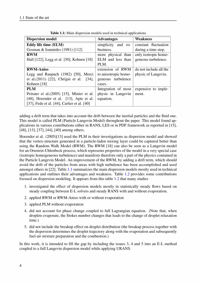
Horender et al. (2005)[13] used the PLM in their investigations as dispersion model and showedthat the vortex-structure generated in a particle-laden mixing layer could be captured better thanusing the Random Walk Model (RWM). The RWM [18] can also be seen as a Langevin modelfor an Ornstein-Uhlenbeck process, which represents properties of the model in a very special case(isotropic homogeneous turbulence) and manifests therefore only a part of the physics contained inthe Particle Langevin Model. An improvement of the RWM, by adding a drift term, which shouldavoid the drift of the particles from areas with high turbulence has been accomplished and usedamongst others in [22]. Table 1.1 summarizes the main dispersion models mostly used in technicalapplications and outlines their advantages and weakness. Table 1.2 provides some contributionsfocused on dispersion modeling. It appears from this table 1.2 that many studies
1. investigated the effect of dispersion models mostly in statistically steady flows based onsteady coupling between E-L solvers and steady RANS with and without evaporation.
2. applied RWM or RWM-Aniso with or without evaporation
3. applied PLM without evaporation
4. did not account for phase change coupled to full Lagrangian equation. (Note that, whendroplets evaporate, the Stokes number changes that leads to the change of droplet relaxationtime.)
5. did not include the breakup effect on droplet distribution (the breakup process together withthe dispersion determines the droplet trajectory along with the evaporation and subsequentlyfuel-air mixture preparation and the combustion.)
In this work, it is intended to fill the gap by including the issues 3, 4 and 5 into an E-L methodcoupled to a full Langevin dispersion model while applying URANS.
4
1 Introduction
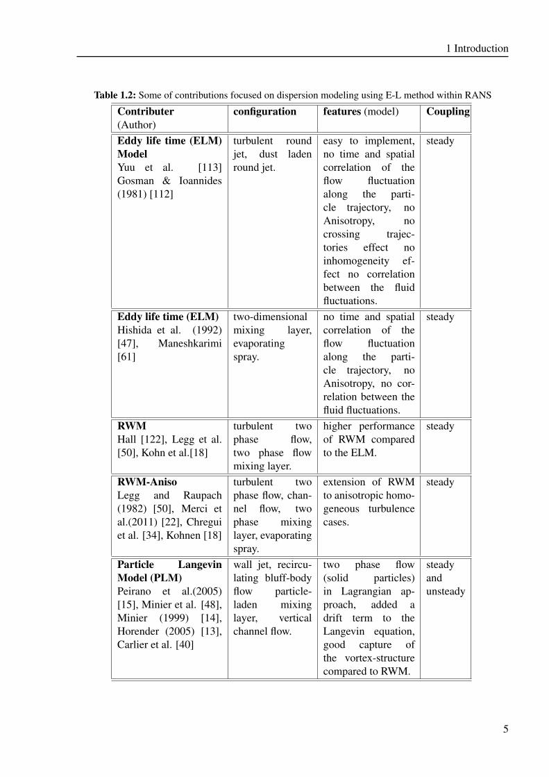
Table 1.2: Some of contributions focused on dispersion modeling using E-L method within RANS
Contributer(Author)
configuration features (model) Coupling
Eddy life time (ELM)ModelYuu et al. [113]Gosman & Ioannides(1981) [112]
turbulent roundjet, dust ladenround jet.
easy to implement,no time and spatialcorrelation of theflow fluctuationalong the parti-cle trajectory, noAnisotropy, nocrossing trajec-tories effect noinhomogeneity ef-fect no correlationbetween the fluidfluctuations.
steady
Eddy life time (ELM)Hishida et al. (1992)[47], Maneshkarimi[61]
two-dimensionalmixing layer,evaporatingspray.
no time and spatialcorrelation of theflow fluctuationalong the parti-cle trajectory, noAnisotropy, no cor-relation between thefluid fluctuations.
steady
RWMHall [122], Legg et al.[50], Kohn et al.[18]
turbulent twophase flow,two phase flowmixing layer.
higher performanceof RWM comparedto the ELM.
steady
RWM-AnisoLegg and Raupach(1982) [50], Merci etal.(2011) [22], Chreguiet al. [34], Kohnen [18]
turbulent twophase flow, chan-nel flow, twophase mixinglayer, evaporatingspray.
extension of RWMto anisotropic homo-geneous turbulencecases.
steady
Particle LangevinModel (PLM)Peirano et al.(2005)[15], Minier et al. [48],Minier (1999) [14],Horender (2005) [13],Carlier et al. [40]
wall jet, recircu-lating bluff-bodyflow particle-laden mixinglayer, verticalchannel flow.
two phase flow(solid particles)in Lagrangian ap-proach, added adrift term to theLangevin equation,good capture ofthe vortex-structurecompared to RWM.
steadyandunsteady
5
1.1 State of the art
1.1.2 Evaporation of droplets
The phase transition (vaporization) is a complex process which has a strong contribution to thephase interaction. Different models have been developed to estimate the rates of heat transfer todroplets and evaporation process in a turbulent ambient. They are generally designed to describetwo main processes in and around the droplets:
1. The droplet models describe the mass and heat transfer phenomena inside the droplet.
2. The phase models are formulated to describe the mass and heat transfer processes betweenthe gas phase surrounding the droplet and the droplet itself.
The infinite heat conductivity model by Ranz & Marshall (1952), the so-called ’D2 Law’ classicalevaporation model by Godsave (1953) and by Spalding (1953) [107] can be representatives of thefirst category of evaporation models, where the surface of the droplets reduce linear with the time.
Regarding the second category, the non-equilibrium model by Bellan &Summerfield (1978) [108]and equilibrium model by Sirignano & Abramzon (1989) are mostly used in investigations ofreacting and non-reacting spray flows. Recent reviews can be found in [125] and [91]. In this workit is assumed that:
1. One component model is considered, so that one solely deals with the so-called infiniteconductivity model.
2. Droplets are assumed to be spherical.
3. Secondary atomization and coalescence of droplets are neglected as one concentrates on thedilute spray region. In other words simple elastic collisions between droplets and wall areassumed without any kind of film formation [12].
4. We neglect the influence of the surface tension and assume a uniform pressure around thedroplet.
5. Uniform physical properties of the surrounding fluid and liquid-vapor thermal equilibriumon the droplet surface.
6. The ambient air is not soluble in the droplet fluid.
7. Chemical reactions and radiation are not considered.
We restrict ourselves to the model by Abramzon and Sirignano [109] who revised the infiniteconductivity model to incorporate the effects of Stefan flow on heat and mass transfer. In thismodel, heat transfer is modified through the use of modified forms for the Nusselt and Sherwoodnumbers.
1.1.3 Spray atomization
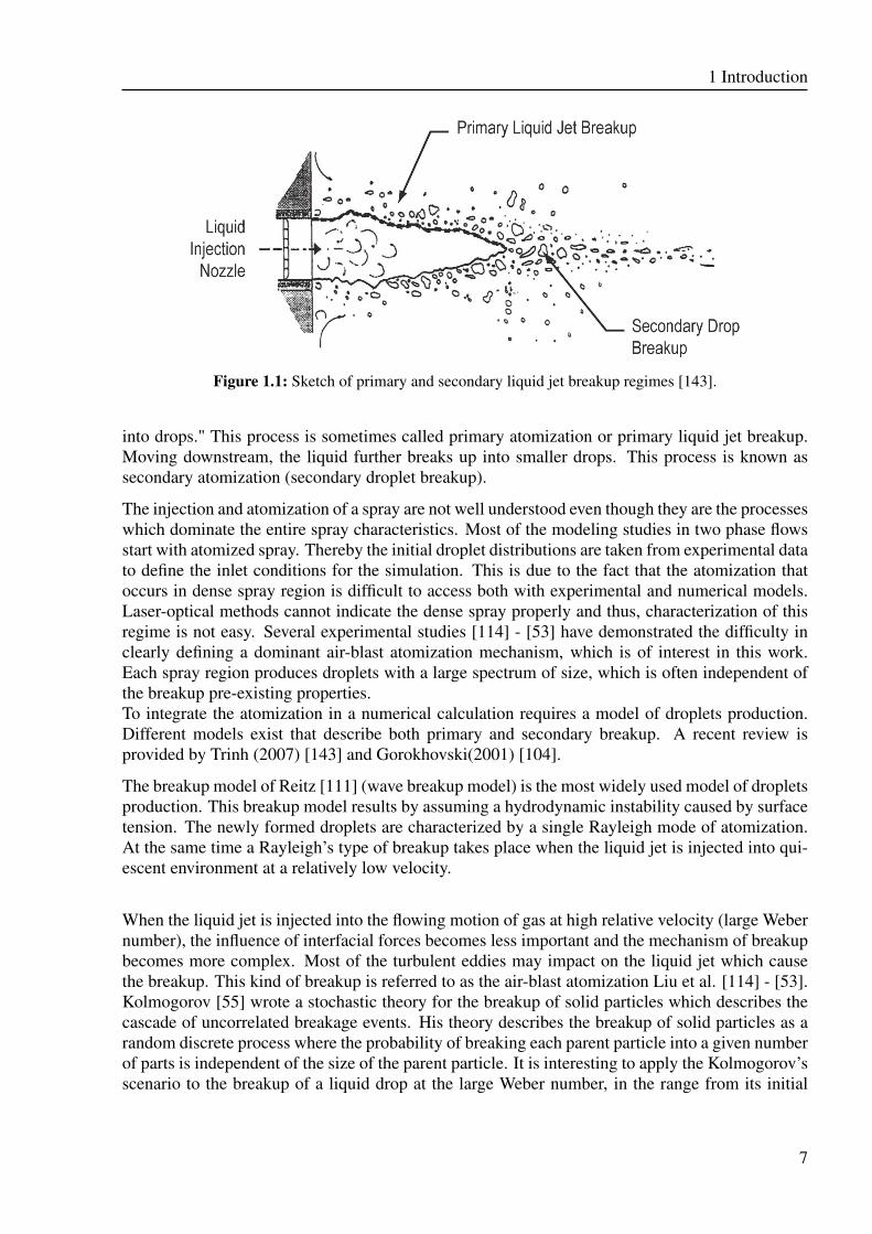
The transformation of a liquid jet into droplet sprays can be divided into two separate steps asshowed in figure 1.1.
The process of the jet breakup is described by Lefebvre [124] as follows: "When a liquid jetemerges from a nozzle as a continuous body of cylindrical form, the competition set up on thesurface of the jet between the cohesive and disruptive forces gives rise to oscillations and pertur-bations. Under favorable conditions the oscillations are amplified and the liquid body disintegrates
6
1 Introduction
Figure 1.1: Sketch of primary and secondary liquid jet breakup regimes [143].
into drops." This process is sometimes called primary atomization or primary liquid jet breakup.Moving downstream, the liquid further breaks up into smaller drops. This process is known assecondary atomization (secondary droplet breakup).
The injection and atomization of a spray are not well understood even though they are the processeswhich dominate the entire spray characteristics. Most of the modeling studies in two phase flowsstart with atomized spray. Thereby the initial droplet distributions are taken from experimental datato define the inlet conditions for the simulation. This is due to the fact that the atomization thatoccurs in dense spray region is difficult to access both with experimental and numerical models.Laser-optical methods cannot indicate the dense spray properly and thus, characterization of thisregime is not easy. Several experimental studies [114] - [53] have demonstrated the difficulty inclearly defining a dominant air-blast atomization mechanism, which is of interest in this work.Each spray region produces droplets with a large spectrum of size, which is often independent ofthe breakup pre-existing properties.To integrate the atomization in a numerical calculation requires a model of droplets production.Different models exist that describe both primary and secondary breakup. A recent review isprovided by Trinh (2007) [143] and Gorokhovski(2001) [104].
The breakup model of Reitz [111] (wave breakup model) is the most widely used model of dropletsproduction. This breakup model results by assuming a hydrodynamic instability caused by surfacetension. The newly formed droplets are characterized by a single Rayleigh mode of atomization.At the same time a Rayleigh’s type of breakup takes place when the liquid jet is injected into qui-escent environment at a relatively low velocity.
When the liquid jet is injected into the flowing motion of gas at high relative velocity (large Webernumber), the influence of interfacial forces becomes less important and the mechanism of breakupbecomes more complex. Most of the turbulent eddies may impact on the liquid jet which causethe breakup. This kind of breakup is referred to as the air-blast atomization Liu et al. [114] - [53].Kolmogorov [55] wrote a stochastic theory for the breakup of solid particles which describes thecascade of uncorrelated breakage events. His theory describes the breakup of solid particles as arandom discrete process where the probability of breaking each parent particle into a given numberof parts is independent of the size of the parent particle. It is interesting to apply the Kolmogorov’sscenario to the breakup of a liquid drop at the large Weber number, in the range from its initial
7
1.1 State of the art
size down to the size of stable droplets once secondary breakup has to be correctly coupled toturbulence. This will be done in this work in order to evaluate the impact of the liquid atomizationon the droplet dispersion process. It should be noted that the cascade idea was involved earlier inthe statistical description of breakup by Novikov et al. [57] where Novikov’s [56] multiplicativeintermittency theory was implemented to obtain the stationary droplet size distribution.
1.1.4 Objectives and outlines of the work
As pointed out above, experience shows that LES has mostly difficulty to deal properly with flowbehavior near the wall. For configurations in which near wall effects are important as it is thecase in wall-bounded multiphase flows, LES will remain too expensive for design and optimiza-tion tasks in various industrial applications notwithstanding the remarkable progress of hardwaretechnologies. In this work it is therefore intended to improve the prediction capability of URANS-based models for wall-bounded multiphase flow configurations featuring complex micro-processesaffected by turbulent dispersion.
As it emerges from Table 1.2 the coupling between phases including the effect of turbulent dis-persion on phase change phenomena and break up process may potentially improve the dropletdistribution prediction once appropriate dispersion models are integrated and an unsteady cou-pling is numerically achieved between involved phases of statically unsteady multiphase flows.For this purpose, the study includes the physical phenomena of
• secondary breakup along with droplet-droplet interactions
• phase change process, especially the droplet evaporation
• full two-way coupling between phases;
all being integrated into an unsteady numerical mode within the URANS context to reliably re-trieve the unsteadiness of turbulent two-phase flows.
Chapter 2 first describes the physical basics of turbulent carrier phase flow without combus-tion. Thereby governing transport equations are outlined along with the turbulence models used.Chapter 3 provides an overview of the essential parameters required for describing the dispersedphase and reviews the main mathematical approaches for numerically studying turbulent two-phaseflows. Chapter 4 sets the theoretical basis for the modeling approach relying on the Eulerian-Lagrangian procedure used in this study. Chapter 5 focuses especially on the modeling of specificprocesses, such as secondary breakup, turbulent dispersion and spray evaporation process. Chapter6 introduces the numerical procedure applied. Two solvers are used for the description of both thegas phase and the dispersed phase. In particular, the numerical coupling between the two solvers,namely the Eulerian and the Lagrangian solver, is shortly highlighted. While the models setupneeds verifications, five different configurations are used for model validation purposes. The abilityof the models to capture the essential multiphase properties is especially evaluated and discussed.The first and second configurations deal with comparison of different dispersion models where thedispersed phase is composed by solid particles without any consideration of phase change or par-ticle heating. The third and fourth configurations include phase change phenomena. In particular,the spray evaporation and the impact of dispersion modeling on the distribution and concentrationof evaporating droplets are analyzed. The last configuration features an air-blast atomization of
8
1 Introduction
interest in modern gas turbine combustors. By forming droplets, a large surface area is produced,that enables to reduce the liquid vaporization time, which results in a better mixing and an increasein the time available for complete combustion [2], [16], [22], [33]. Since experience shows thatatomization results depend on the atomizer design and are difficult to be compared to each other,there is a need for directly predicting the outcome of the atomization process. This may dispensewith the need to perform empirical studies for each individual atomizer geometry and will helpinitialize safety the droplet numerical tracking calculations. The main idea behind this task is toascertain the predictability of a stochastic model together with its impact on the turbulent dropletdispersion. This manuscript is closed by chapter 8 that summarizes the main findings of this studyand suggests possible directions for future research
9

2 Fundamentals of turbulent flows
2.1 The scales of turbulent motion
Turbulent flows are characterized by different flow structure sizes. The large but not the largesteddies contain major part of the turbulent kinetic energy. Due to this fact the large eddies areoften called as energy containing eddies. The length and time scales of these eddies are of inter-est. In particular the size of the energy containing eddies depends on the geometry of a spatialdomain as well as the local intensity of turbulence. This size can be related to the integral turbulentlength scale that can be determined from the two-point spatial correlation function or coefficientfor statistically steady (time independent) turbulence
RLij(x, x+ ∆x) =
ui(x)uj(x+ ∆x)√ui
2(x)
√ui
2(x+ ∆x)
(2.1)
Lij =1
2
∫ +∞
−∞RLij(x, x+ ∆x)d(∆x) (2.2)
Here Lij is the length scale tensor. For homogeneous isotropic turbulence the integral length scale,which is independent of the direction, is given by
lt =1
3Lii (2.3)
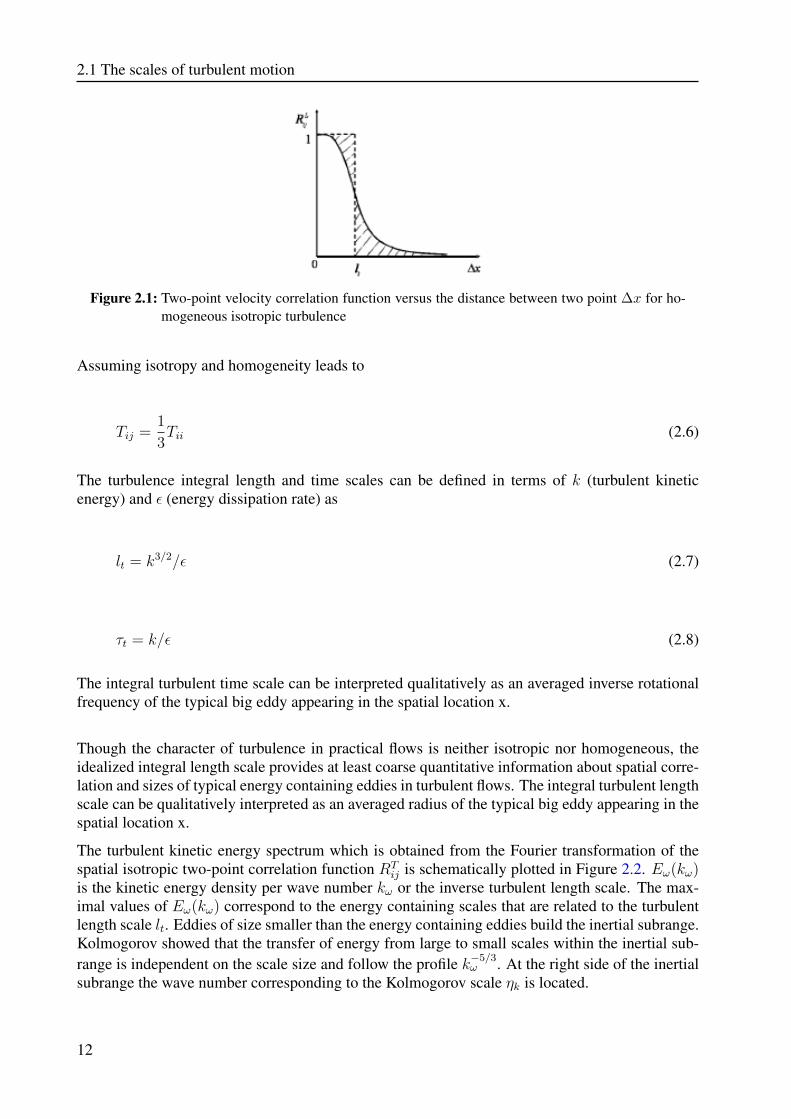
The two-point velocity correlation function for homogeneous isotropic turbulence and the corre-sponding integral turbulent length scale are schematically shown in Figure 2.1.
The corresponding time scale can be determined from the known time correlation function
RTij(x, t+ ∆t) =
ui(t)uj(t+ ∆t)√ui
2(t)
√ui
2(t+ ∆t)
(2.4)
Tij =1
2
∫ +∞
−∞RTij(x, t, t+ ∆t)d(∆t) (2.5)
11
2.1 The scales of turbulent motion
Figure 2.1: Two-point velocity correlation function versus the distance between two point ∆x for ho-mogeneous isotropic turbulence
Assuming isotropy and homogeneity leads to
Tij =1
3Tii (2.6)
The turbulence integral length and time scales can be defined in terms of k (turbulent kineticenergy) and ε (energy dissipation rate) as
lt = k3/2/ε (2.7)
τt = k/ε (2.8)
The integral turbulent time scale can be interpreted qualitatively as an averaged inverse rotationalfrequency of the typical big eddy appearing in the spatial location x.
Though the character of turbulence in practical flows is neither isotropic nor homogeneous, theidealized integral length scale provides at least coarse quantitative information about spatial corre-lation and sizes of typical energy containing eddies in turbulent flows. The integral turbulent lengthscale can be qualitatively interpreted as an averaged radius of the typical big eddy appearing in thespatial location x.
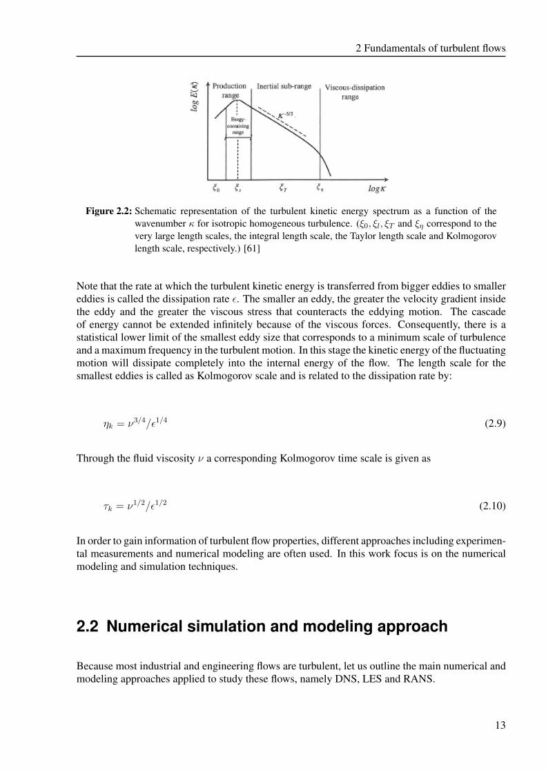
The turbulent kinetic energy spectrum which is obtained from the Fourier transformation of thespatial isotropic two-point correlation function RT
ij is schematically plotted in Figure 2.2. Eω(kω)is the kinetic energy density per wave number kω or the inverse turbulent length scale. The max-imal values of Eω(kω) correspond to the energy containing scales that are related to the turbulentlength scale lt. Eddies of size smaller than the energy containing eddies build the inertial subrange.Kolmogorov showed that the transfer of energy from large to small scales within the inertial sub-range is independent on the scale size and follow the profile k−5/3
ω . At the right side of the inertialsubrange the wave number corresponding to the Kolmogorov scale ηk is located.
12
2 Fundamentals of turbulent flows
Figure 2.2: Schematic representation of the turbulent kinetic energy spectrum as a function of thewavenumber κ for isotropic homogeneous turbulence. (ξ0, ξl, ξT and ξη correspond to thevery large length scales, the integral length scale, the Taylor length scale and Kolmogorovlength scale, respectively.) [61]
Note that the rate at which the turbulent kinetic energy is transferred from bigger eddies to smallereddies is called the dissipation rate ε. The smaller an eddy, the greater the velocity gradient insidethe eddy and the greater the viscous stress that counteracts the eddying motion. The cascadeof energy cannot be extended infinitely because of the viscous forces. Consequently, there is astatistical lower limit of the smallest eddy size that corresponds to a minimum scale of turbulenceand a maximum frequency in the turbulent motion. In this stage the kinetic energy of the fluctuatingmotion will dissipate completely into the internal energy of the flow. The length scale for thesmallest eddies is called as Kolmogorov scale and is related to the dissipation rate by:
ηk = ν3/4/ε1/4 (2.9)
Through the fluid viscosity ν a corresponding Kolmogorov time scale is given as
τk = ν1/2/ε1/2 (2.10)
In order to gain information of turbulent flow properties, different approaches including experimen-tal measurements and numerical modeling are often used. In this work focus is on the numericalmodeling and simulation techniques.
2.2 Numerical simulation and modeling approach
Because most industrial and engineering flows are turbulent, let us outline the main numerical andmodeling approaches applied to study these flows, namely DNS, LES and RANS.
13
2.2 Numerical simulation and modeling approach
2.2.1 Direct numerical simulation (DNS)
The Navier-Stokes equations that describe the motion of any Newtonian fluid can be numericallysolved by means of the DNS (direct numerical simulation) approach without any turbulence model.Thereby the whole range of spatial and temporal scales of the turbulence must be resolved.
By doing this the computational cost of DNS becomes very high, especially for the high Reynoldsnumbers flows in most industrial applications. Nevertheless, direct numerical simulation is of-ten used in fundamental research in turbulence for low and moderate Reynolds number flows.Thereby DNS allows a wide understanding of the physics of turbulence. Therefore, using DNSmake it possible to perform variable "numerical experiments", since one can extract from DNSdata information which are difficult or impossible to obtain in measurement experiments. Thus,direct numerical simulations are useful in the development of turbulence models for practical ap-plications, such as sub-grid scale models for Large eddy simulation (LES) and turbulence modelsfor methods that solve the Reynolds-averaged Navier-Stokes equations (RANS). This is accom-plished by means of "a priori" tests, in which the input data for the model is taken from a DNSsimulation, or by "a posteriori" tests, in which the results produced by the model are comparedwith those obtained by DNS.
2.2.2 Large eddy simulation (LES)
Large eddy simulation consists in a direct computing of large eddies and modeling of small (quasi-universal) eddies so-called subgrid scales (SGS). In this method, not the whole turbulent spectrumhas to be resolved. It uses a filtering operation that allows for removing in a proper way the smallscales. This operation introduces new unknown terms representing the small-scale informationlost by the filtering. Thus, some models for the small scales called as SGS-models are needed inorder to close the system of filtered equations. From the modeling point of view this approachsimply displaces the problem into the less important part of the energy spectrum. As a subgridparameterization is still necessary, its influence is expected to be rather small, at least when themost important scales are all resolved on the computational grid.
Because in LES small eddies are modeled, computational grid will be therefore much bigger thanthe Kolmogorov length scale, and time steps can be chosen much bigger than in DNS. So thecomputing resources for LES are much lower than DNS. The area of applications of LES has con-siderably increased with rapid development of computer facilities. However, some problems areinborn to LES. For example, the problem of wall flows is still not satisfactory solved. It is apparentthat near the wall all vortices are small so that both space and time steps needed for LES dropdown to values which is characteristic for DNS. Existing solutions such as anisotropic models anddynamic procedures, still not give satisfactory results.For numerical combustion investigations, some optimism has appeared among researchers, whobelieve to overcome the problems of turbulence modeling by means of LES [130]. However, inaddition to difficulties in handling the flow in the vicinity of solid boundaries, LES still requiresturbulent combustion models for the SGS part. The development of these models for LES and theirapplication to various reacting flows appears to be the most popular area of modern combustionresearch, but most models are still based on RANS type concepts. One of the solution for thewall problem for LES appears to be a combination of LES and the Reynolds averaging numericalsimulation (here RANS) in the line of the so-called hybrid RANS/LES models. The latter method
14
2 Fundamentals of turbulent flows
will be addressed later on.
2.2.3 Reynolds averaged numerical simulation (RANS) method
Previously known as Reynolds averaged Navier-Stokes method, today the Reynolds averagingprocedure is extended to quantities in all scalar (passive or reactive) transport equations. TheRANS method was thought of most prevalently used statistical solution approach for scientific andengineering calculations and was mostly developed during the last decades. Its economical com-putational cost and its good performance near walls makes it the basis of numerical investigationin the present study.
In the RANS approach the turbulent flow is modeled over the whole range of small and largescales, and governing equations are solved for mean field quantities. In this Reynolds averagingconcept, each instantaneous variable φ of the turbulent flow field is therefore considered to be thesum of a mean value φ and its fluctuation φ,
φ(xi, t) = φ(xi, t) + φ(xi, t), (2.11)
The mean value φ can be obtained from a statistical averaging. It may be, for instance, an ensembleaveraging that is taken over a sufficiently large number N of experiments having the same initialand boundary conditions,
φ(xi, t) =1
N
N∑n=1
φn(xi, t). (2.12)
Alternatively, simple time-averaging can be used to provide statistical average values. For timedepending mean variable in a period ∂t with t2 = t1 + ∂t, the time-averaged variable is defined as
φ(xi, t) =1
∂t
t+∂t∑t
φ(xi, t)dt, (2.13)
and the mean of fluctuating part is then set to zero,
φ = 0. (2.14)
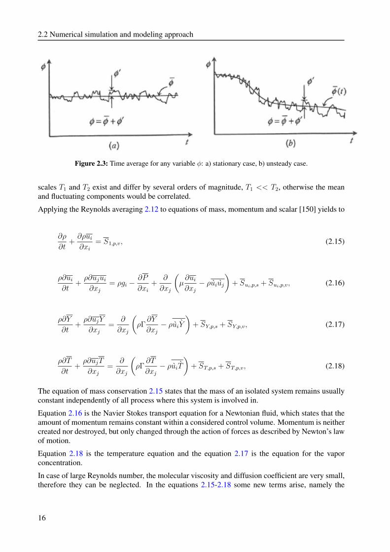
In Fig. 2.3 the decomposition of a general variable φ as a function of time is shown for a stationaryand unsteady flow, respectively.
In this time-averaging concept, a separation of the fluctuating time scales of variables, T1, and themain time scale of the ’slow’ variation of mean flow, T2, is assumed. This means that the time
15
2.2 Numerical simulation and modeling approach
Figure 2.3: Time average for any variable φ: a) stationary case, b) unsteady case.
scales T1 and T2 exist and differ by several orders of magnitude, T1 << T2, otherwise the meanand fluctuating components would be correlated.
Applying the Reynolds averaging 2.12 to equations of mass, momentum and scalar [150] yields to
∂ρ
∂t+∂ρui∂xi
= S1,p,v, (2.15)
ρ∂ui∂t
+ρ∂ujui∂xj
= ρgi −∂P
∂xi+
∂
∂xj
(µ∂ui∂xj− ρuiuj
)+ Sui,p,s + Sui,p,v, (2.16)
ρ∂Y
∂t+ρ∂ujY
∂xj=
∂
∂xj
(ρΓ
∂Y
∂xj− ρuiY
)+ SY,p,s + SY,p,v, (2.17)
ρ∂T
∂t+ρ∂ujT
∂xj=
∂
∂xj
(ρΓ
∂T
∂xj− ρuiT
)+ ST,p,s + ST,p,v, (2.18)
The equation of mass conservation 2.15 states that the mass of an isolated system remains usuallyconstant independently of all process where this system is involved in.
Equation 2.16 is the Navier Stokes transport equation for a Newtonian fluid, which states that theamount of momentum remains constant within a considered control volume. Momentum is neithercreated nor destroyed, but only changed through the action of forces as described by Newton’s lawof motion.
Equation 2.18 is the temperature equation and the equation 2.17 is the equation for the vaporconcentration.
In case of large Reynolds number, the molecular viscosity and diffusion coefficient are very small,therefore they can be neglected. In the equations 2.15-2.18 some new terms arise, namely the
16
2 Fundamentals of turbulent flows
unclosed Reynolds stress tensor uiuj the turbulent transport terms ujY and ujT which have to bemodeled. The last type of unclosed quantities, in the right hand side represent the particles/dropletssource terms which in turn will be explained in details later.
Although the main advantages of RANS are the relatively low computational costs involved andthe wide range of applicability compared to DNS or LES, from an accuracy point of view RANSmodeling lies below DNS and LES and the effort required to model the whole energy spectrumincluding large and small scale structures is higher [128].
2.3 Modeling Reynolds stresses
Focused on the mean flow description2.15 - 2.18 turbulence modeling aims at representing theunclosed terms as realistically as possible. In the following first order turbulence models, as theyare used within this work, will be introduced.
2.3.1 First order turbulence modeling and k-ε two-equationsmodeling
For the description of the unknown Reynolds stresses Boussinesq proposed the first assumption(isotropic turbulence) [79] by introducing the correlation 2.19, which gave rise to the first orderturbulence modeling.
−u′iu′j = νt
(∂ui∂xj
+∂uj∂xi
)− 2
3kδij, (2.19)
k = 1/2u′iu′i the turbulent kinetic energy and νt represents the eddy viscosity. The Reynolds stress
tensor modeled by means of such velocity gradients-ansatz, can be legitimated for applicationswith a flow dominant direction like turbulent channel or shear flow.
Representing the turbulent length and time scales, respectively k and ε quantities have been usedto represent mathematically the eddy viscosity νt. In 1974 Launder and Spalding introduced thefamous standard k− ε two equation turbulence model [133], where the turbulent eddy viscosity νtis related to k and ε , through the following semi-empirical expression:
νt = Cµk2
ε, (2.20)
where Cµ (see Table 2.1) is a model constant and k and ε are determined by their respectivecoordinate-invariant modeled transport equations.
∂k
∂t+
∂
∂xi(uik) = − ∂
∂xi
(νtσk
∂k
∂xi
)− u′iu′j
∂uj∂xj− ε (2.21)
17
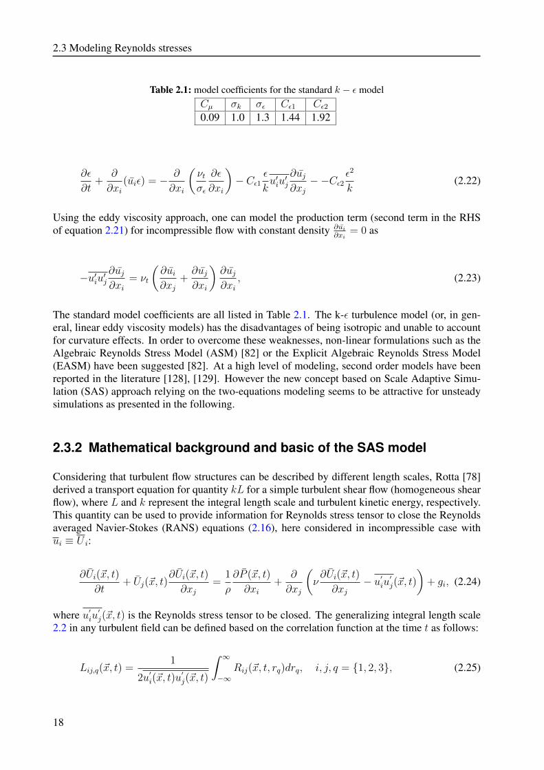
2.3 Modeling Reynolds stresses
Table 2.1: model coefficients for the standard k − ε modelCµ σk σε Cε1 Cε20.09 1.0 1.3 1.44 1.92
∂ε
∂t+
∂
∂xi(uiε) = − ∂
∂xi
(νtσε
∂ε
∂xi
)− Cε1
ε
ku′iu′j
∂uj∂xj−−Cε2
ε2
k(2.22)
Using the eddy viscosity approach, one can model the production term (second term in the RHSof equation 2.21) for incompressible flow with constant density ∂ui
∂xi= 0 as
−u′iu′j∂uj∂xi
= νt
(∂ui∂xj
+∂uj∂xi
)∂uj∂xi
, (2.23)
The standard model coefficients are all listed in Table 2.1. The k-ε turbulence model (or, in gen-eral, linear eddy viscosity models) has the disadvantages of being isotropic and unable to accountfor curvature effects. In order to overcome these weaknesses, non-linear formulations such as theAlgebraic Reynolds Stress Model (ASM) [82] or the Explicit Algebraic Reynolds Stress Model(EASM) have been suggested [82]. At a high level of modeling, second order models have beenreported in the literature [128], [129]. However the new concept based on Scale Adaptive Simu-lation (SAS) approach relying on the two-equations modeling seems to be attractive for unsteadysimulations as presented in the following.
2.3.2 Mathematical background and basic of the SAS model
Considering that turbulent flow structures can be described by different length scales, Rotta [78]derived a transport equation for quantity kL for a simple turbulent shear flow (homogeneous shearflow), where L and k represent the integral length scale and turbulent kinetic energy, respectively.This quantity can be used to provide information for Reynolds stress tensor to close the Reynoldsaveraged Navier-Stokes (RANS) equations (2.16), here considered in incompressible case withui ≡ U i:
∂Ui(~x, t)
∂t+ Uj(~x, t)
∂Ui(~x, t)
∂xj=
1
ρ
∂P (~x, t)
∂xi+
∂
∂xj
(ν∂Ui(~x, t)
∂xj− u′
iu′j(~x, t)
)+ gi, (2.24)
where u′iu
′j(~x, t) is the Reynolds stress tensor to be closed. The generalizing integral length scale
2.2 in any turbulent field can be defined based on the correlation function at the time t as follows:
Lij,q(~x, t) =1
2u′i(~x, t)u
′j(~x, t)
∫ ∞−∞
Rij(~x, t, rq)drq, i, j, q = {1, 2, 3}, (2.25)
18
2 Fundamentals of turbulent flows
where u′i andRij are velocity fluctuation and the correlation functions, respectively. ~x and ~r denote
position vector in the flow field and displacement vector between two points in the flow field. Theoverbar denotes the ensemble averaging. Rij is defined as below:
Rij(~x,~r, t) = u′i(~x, t)u
′j(~x+ ~r, t). (2.26)
Note that its normalized expression leads to the correlation coefficient (here correlation function)in 2.2. In equation 2.25, q denotes the direction of integration, say stream wise (x1), normal (x2) orspan wise (x3). Regarding shear flows, Rotta[78] assumed a simplified form for the integral lengthscale as follows:
Ψ = k(~x)L(~x) =3
16
∫ ∞−∞
Rii(~x, rx2)drx2 , (2.27)
where x2 denotes the shear strain direction and 316
is a scaling factor enabling to capture theisotropic limit.Rotta[78] then derived a transport equation for Ψ regarding homogeneous turbulent shear flows byintegrating the simplified transport equation of Rij in rx2 direction. This then then appeared in thefollowing form:
U1(~x)∂Ψ
∂x1
+ U2(~x)∂Ψ
∂x2
= (2.28)
− u′1u
′2(~x)
(ξ1L(~x)
∂U1(~x)
∂x2
+ ξ2L2(~x)
∂2U1(~x)
∂x22
+ ξ3L3(~x)
∂3U1(~x)
∂x32
)− ccLk(~x)
32 +
∂
∂x2
{kL√k(~x)L
[L(~x)
∂k(~x)
∂x2
+ αLk(~x)∂L(~x)
∂x2
]}.
Rotta[78] proposed the value 1.2 for ξ1 based on measurements for a homogeneous shear flowperformed by Rose [137], while the other remaining model constants will be determined later.Due to the axisymmetric behavior of R12 in homogeneous shear flows the Rotta’s transport equa-tion does not include the term with second velocity derivative . Therefore, the final transportequation proposed by Rotta[78] for homogeneous shear followed from equation 2.29 as below:
U1(~x)∂Ψ
∂x1
+ U2(~x)∂Ψ
∂x2
= (2.29)
− u′1u
′2(~x)
(ξ1L(~x)
∂U1(~x)
∂x2
+ ξ3L3(~x)
∂3U1(~x)
∂x32
)− ccLk(~x)
32 +
∂
∂x2
{kL√k(~x)L
[L(~x)
∂k(~x)
∂x2
+ αLk(~x)∂L(~x)
∂x2
]}.
Where ξ1, ξ3 are model constants. Three observations need to be pointed out. First, symmetry con-siderations (see [130]) showed that in the case of wall bounded flows with no symmetry breaking
19
2.3 Modeling Reynolds stresses
condition the third velocity derivative is vanishing and the term with second velocity derivative isremaining. Second, for complex shear flows with symmetry breaking conditions both terms arepresent. However, in this study following transport equation regarding wall bounded shear flowswill be considered.
U1(~x)∂Ψ
∂x1
+ U2(~x)∂Ψ
∂x2
= (2.30)
− u′1u
′2(~x)
(ξ1L(~x)
∂U1(~x)
∂x2
+ ξ2L2(~x)
∂2U1(~x)
∂x22
)− ccLk(~x)
32 +
∂
∂x2
{kL√k(~x)L
[L(~x)
∂k(~x)
∂x2
+ αLk(~x)∂L(~x)
∂x2
]},
where the term including third derivative has not been included due to requirement of particularnumerical treatment. Third, as mentioned before, Rotta’s transport equation has been derived forhomogeneous shear flows based on local isotropy concepts. These concepts are only legitimatefor regions away from the wall (very high Reynolds number) where the cascade process occurs.However, information for the Reynolds stress tensor to close the RANS equations is needed forthe whole domain. Therefore, a novel combination of modified form of equation 2.31 concerningcomplex three dimensional shear flows together with an appropriate near wall turbulence modelwould be a reasonable approach. Menter et al.[141] proposed a seamless hybrid approach using amodified form of equation 2.30 and denoted it as SST − SAS model.for brevity reasons note that from now on in the rest of this section the variable (~x) is dropped fromthe quantities.
The SST − SAS model: Based solely on the dimensional analysis, Menter et al. [141] modifiedand simplified equation 2.30 as follows:
U1∂Ψ
∂x1
+ U2∂Ψ
∂x2
=Ψ
kPk
(ξ1 + ξ2
(L
Lvk
)2)− ξ3k
32 +
∂
∂x2
{νtσΨ
∂Ψ
∂x2
}, (2.31)
where Lvk denotes the von-Karman length scale
(L = 0.41
∂U1∂x2∂2U1∂x2
2
)
and Pk the production of
turbulent kinetic energy(Pk = −u′
1u′2∂U1
x2
).
The first term on the right hand side models the production, the second term dissipation and thethird term postulates the diffusion using simple gradient approach.To apply equation 2.31 to complex flows, an evaluation of the first and second derivatives in L isneeded. For this purpose, Menter et al.[141] defined following norms for the first and the secondderivatives of velocity:
‖U ′‖= S =√
2SijSij; Sij =1
2
(∂Ui∂xj
+∂Uj∂xi
).
20
2 Fundamentals of turbulent flows
‖U ′′‖=
√∂2Ui∂xj∂xj
∂2Ui∂xk∂xk
; Lvk = 0.41
∣∣∣∣U ′
U ′′
∣∣∣∣ .Instead of equation for kL, Menter et al.[141] transformed the transport equation 2.31 to a one withnew variable Φ =
√kL and proposed following two-equations model for complex (3-dimensional)
flows called K square-root-KL (KSKL) model :
∂k
∂t+ Uj
∂k
∂xj= Pk − c0.75
µ
k2
Φ+
∂
∂xj
(νtσk
∂k
∂xj
)(2.32)
∂Φ
∂t+ Uj
∂Φ
∂xj=
Φ
kPk
(ζ1 − ζ2
(L
Lvk
)2)− ζ3k +
∂
∂xj
(νtσΦ
∂Φ
∂xj
)(2.33)
νt = c14µΦ, Φ =
√kL ζ1 = 0.8, ζ2 = 1.47, ζ3 = 0.028, σk = σΦ = 2/3.
The KSKL model was transformed into K − ω (ω = εk) framework resulting in an additional term
in the transport equation for ω given as below:
QSAS = max
[ζ2S
2
(L
Lvk
)− CSAS
2k
σΦ
max
(1
k2
∂k
∂xj
∂k
∂xj,
1
ω2
∂ω
∂xj
∂ω
∂xj
), 0
], (2.34)
with CSAS = 2. This term has been added to the ω transport equation of the k − ω − SST model[127]. Where the max function and the k−derivative term have been empirically introduced toavoid numerical instability of the model regarding attached flows.With respect to this modeling approach some observations can be pointed out:
1. According to the finding of [128], the SST − SAS model has shortcomings dealing with flowslike diffuser, hill flow and channel flow, where the flow instabilities are relatively weak.
2. In the forms of hybride LES/RANS it should be noted that neither SST − SAS nor DDES(delayed detached Eddy simulation) are able to switch from RANS to scale resolving mode with-out an explicit introduction of synthetic turbulence. This might be due to the used norm for thesecond derivative of the velocity and the resulting additional source terms, that are responsible forthe scale adaptivity of resolution.
Modified SAS approach by Mehdizadeh et al. [144]The approach is to consider a continuum-mechanics consistent norm and then to introduce a zonalapproach in order to accommodate in a consistent way the near wall turbulence treatment and thefeatures of equation 2.30.
The source term of the equation 2.30 includes first and second derivative of velocity which issimilar to the Von-Karman relationship. Therefore, the equation constants have to be determined,so that the equation in the limiting case returns the Von-Karman relationship for integral length
21
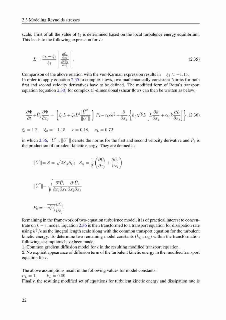
2.3 Modeling Reynolds stresses
scale. First of all the value of ξ2 is determined based on the local turbulence energy equilibrium.This leads to the following expression for L:
L =cL − ξ1
ξ2
∂U1
∂x2
∂2U1
∂x22
. (2.35)
Comparison of the above relation with the von-Karman expression results in ξ2 ≈ −1.15.In order to apply equation 2.35 to complex flows, two mathematically consistent Norms for bothfirst and second velocity derivatives have to be defined. The modified form of Rotta’s transportequation (equation 2.30) for complex (3-dimensional) shear flows can then be written as below:
∂Ψ
∂t+Uj
∂Ψ
∂xj=
ξ1L+ ξ2L2‖U
′′‖‖U ′‖
Pk−cLck32 +
∂
∂xj
{kL√kL
[L∂k
∂xj+ αLk
∂L
∂xj
]}(2.36)
ξ1 = 1.2, ξ2 = −1.15, c = 0.18, cL = 0.72
in which 2.36, ‖U ′‖, ‖U ′′‖ denote the norms for the first and second velocity derivative and Pk isthe production of turbulent kinetic energy. They are defined as:
‖U ′‖= S =√
2SijSij; Sij =1
2
(∂Ui∂xj
+∂Uj∂xi
)
‖U ′′‖=
√∂2Ui∂xj∂xk
∂2Ui∂xj∂xk
Pk = −u′iu
′j
∂Ui∂xj
.
Remaining in the framework of two-equation turbulence model, it is of practical interest to concen-trate on k− ε model. Equation 2.36 is then transformed to a transport equation for dissipation rateusing k
32/ε as the integral length scale along with the common transport equation for the turbulent
kinetic energy. To determine two remaining model constants (kL , αL) within the transformationfollowing assumptions have been made:1. Common gradient diffusion model for ε in the resulting modified transport equation.2.No explicit appearance of diffusion term of the turbulent kinetic energy in the modified transportequation for ε.
The above assumptions result in the following values for model constants:αL = 1, kL = 0.09.Finally, the resulting modified set of equations for turbulent kinetic energy and dissipation rate is
22
2 Fundamentals of turbulent flows
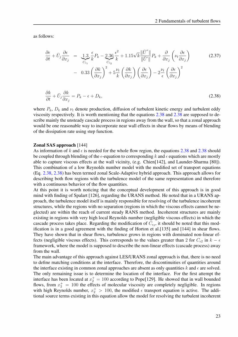
as follows:
∂ε
∂t+ Uj
∂ε
∂xj= 1.3︸︷︷︸
Cε1
ε
kPk − 2.36︸︷︷︸
Cε2
ε2
k+ 1.15
√k‖U ′′‖‖U ′‖
Pk +∂
∂xj
(νt∂ε
∂xj
)(2.37)
− 0.33
(∂k
∂xj
)2
+ 5νtk
(∂k
∂xj
)(∂ε
∂xj
)− 2
νtε
(∂ε
∂xj
)2
∂k
∂t+ Uj
∂k
∂xj= Pk − ε+Dk, (2.38)
where Pk, Dk and νt denote production, diffusion of turbulent kinetic energy and turbulent eddyviscosity respectively. It is worth mentioning that the equations 2.38 and 2.38 are supposed to de-scribe mainly the unsteady cascade process in regions away from the wall, so that a zonal approachwould be one reasonable way to incorporate near wall effects in shear flows by means of blendingof the dissipation rate using step function.
Zonal SAS approach [144]As information of k and ε is needed for the whole flow region, the equations 2.38 and 2.38 shouldbe coupled through blending of the ε-equation to corresponding k and ε equations which are mostlyable to capture viscous effects at the wall vicinity, (e.g. Chien[142], and Launder-Sharma [80]).This combination of a low Reynolds number model with the modified set of transport equations(Eq. 2.38, 2.38) has been termed zonal Scale-Adaptive hybrid approach. This approach allows fordescribing both flow regions with the turbulence model of the same representation and thereforewith a continuous behavior of the flow quantities.At this point it is worth noticing that the conceptual development of this approach is in goodmind with finding of Spalart [126], regarding the URANS method. He noted that in a URANS ap-proach, the turbulence model itself is mainly responsible for resolving of the turbulence incoherentstructures, while the regions with no separation (regions in which the viscous effects cannot be ne-glected) are within the reach of current steady RANS method. Incoherent structures are mainlyexisting in regions with very high local Reynolds number (negligible viscous effects) in which thecascade process takes place. Regarding the modification of Cε2 , it should be noted that this mod-ification is in a good agreement with the finding of Horton et al.[135] and [144] in shear flows.They have shown that in shear flows, turbulence grows in regions with dominated non-linear ef-fects (negligible viscous effects). This corresponds to the values greater than 2 for Cε2 in k − εframework, where the model is supposed to describe the non-linear effects (cascade process) awayfrom the wall.The main advantage of this approach against LES/URANS zonal approach is that, there is no needto define matching conditions at the interface. Therefore, the discontinuities of quantities aroundthe interface existing in common zonal approaches are absent as only quantities k and ε are solved.The only remaining issue is to determine the location of the interface. For the first attempt theinterface has been located at x+
2 = 100 according to Pope[129]. He showed that in wall boundedflows, from x+
2 = 100 the effects of molecular viscosity are completely negligible. In regionswith high Reynolds number, x+
2 > 100, the modified ε transport equation is active. The addi-tional source terms existing in this equation allow the model for resolving the turbulent incoherent
23
2.3 Modeling Reynolds stresses
structures, while the near wall turbulence model returns a steady RANS solution for the near wallregion. More details of this model can be found in [144].
24
3 Multiphase flow properties anddescription approaches
3.1 Relevant parameter characterizing dispersed phaseflows
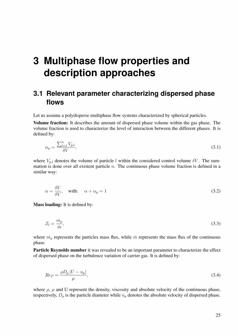
Let us assume a polydisperse multiphase flow systems characterized by spherical particles.
Volume fraction: It describes the amount of dispersed phase volume within the gas phase. Thevolume fraction is used to characterize the level of interaction between the different phases. It isdefined by:
αp =
∑nl=1 Vp,lδV
, (3.1)
where Vp,l denotes the volume of particle l within the considered control volume δV . The sum-mation is done over all existent particle n. The continuous phase volume fraction is defined in asimilar way:
α =δV
δV, with: α + αp = 1 (3.2)
Mass loading: It is defined by:
Zl =mp
m, (3.3)
where mp represents the particles mass flux, while m represents the mass flux of the continuousphase.
Particle Reynolds number it was revealed to be an important parameter to characterize the effectof dispersed phase on the turbulence variation of carrier gas. It is defined by:
ReP =ρDp |U − up|
µ, (3.4)
where ρ, µ and U represent the density, viscosity and absolute velocity of the continuous phase,respectively, Dp is the particle diameter while up denotes the absolute velocity of dispersed phase.
25
3.2 Main Multi-phase Flow Approaches
Particle relaxation time: defines the ability of a given particle to react to the carrier gas. The parti-cle relaxation time yields the time taken by a particle to respond on the fluid velocity modification.It is defined by:
τp =ρpD
2p
18µ, (3.5)
where ρp is the particle density.
Stokes number: measures the inertia of one particle. It is defined as the ratio of the particlerelaxation time to the turbulent time scale. The Stokes number is important in order to characterizeinteraction processes with the particle (such as separation, deposition, modulation, etc.)
St =τpTch
, (3.6)
where Tch denotes the turbulent characteristic time scale.
3.2 Main Multi-phase Flow Approaches
The numerical methods used in solving dispersed multi-phase flows are basically classified in threecategories:
1. The Eulerian Lagrangian method treats the fluid as a continuum and the particles as discreteentities.
2. The two-fluid method treats the particle phase and carrier phase as interpenetrating and in-teracting continuum.
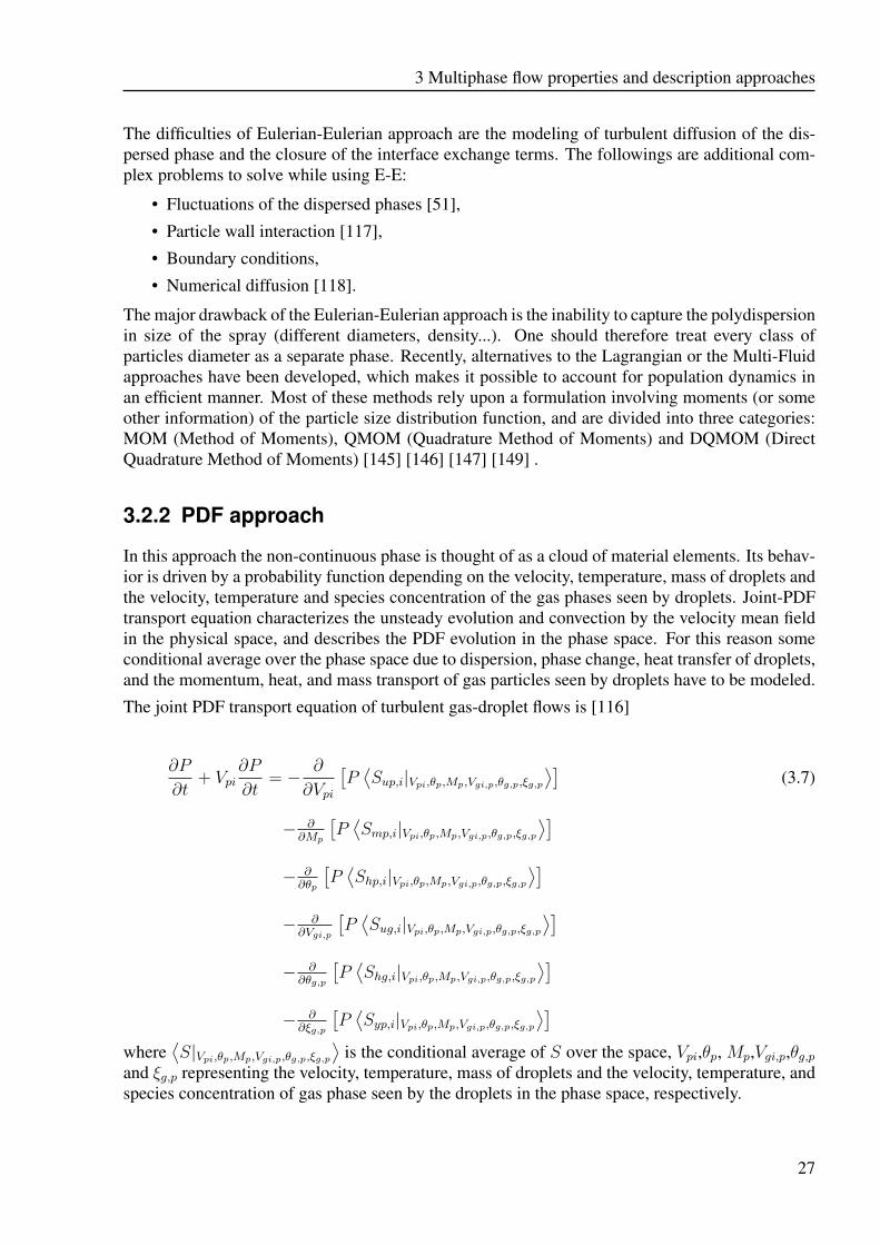
3. The Probability Density Function (PDF) method describes the flows by the joint statisticalproperties of the gas phase properties and the droplet properties.
3.2.1 Eulerian Eulerian approach
The classical two-fluid models have been the subject of many publications either in the mathemat-ics community [115] or in the engineering one [51]. The Eulerian-Eulerian (E-E) approach treatsboth phases as continua. The behavior of dispersed and gas phase is characterized by using partialdifferential transport equations which describe the flow of the fluids. This approach is more suit-able in case of dense two-phase flow in which the volume fraction of both phases may be greaterthan 10−3. Such a formulation for both phases lends itself more naturally to parallel computingand transient flow calculations. The reason behind this is that parallel numerical computation isachieved by arranging fluid-blocks to CPU and not particles. The multiple dispersed phases havesimilar transport equations as the gas phase which makes the implementation not very complex.The coupling between two phases is easily done and the convergence criteria can be clearly defined[51].
26
3 Multiphase flow properties and description approaches
The difficulties of Eulerian-Eulerian approach are the modeling of turbulent diffusion of the dis-persed phase and the closure of the interface exchange terms. The followings are additional com-plex problems to solve while using E-E:
• Fluctuations of the dispersed phases [51],
• Particle wall interaction [117],
• Boundary conditions,
• Numerical diffusion [118].
The major drawback of the Eulerian-Eulerian approach is the inability to capture the polydispersionin size of the spray (different diameters, density...). One should therefore treat every class ofparticles diameter as a separate phase. Recently, alternatives to the Lagrangian or the Multi-Fluidapproaches have been developed, which makes it possible to account for population dynamics inan efficient manner. Most of these methods rely upon a formulation involving moments (or someother information) of the particle size distribution function, and are divided into three categories:MOM (Method of Moments), QMOM (Quadrature Method of Moments) and DQMOM (DirectQuadrature Method of Moments) [145] [146] [147] [149] .
3.2.2 PDF approach
In this approach the non-continuous phase is thought of as a cloud of material elements. Its behav-ior is driven by a probability function depending on the velocity, temperature, mass of droplets andthe velocity, temperature and species concentration of the gas phases seen by droplets. Joint-PDFtransport equation characterizes the unsteady evolution and convection by the velocity mean fieldin the physical space, and describes the PDF evolution in the phase space. For this reason someconditional average over the phase space due to dispersion, phase change, heat transfer of droplets,and the momentum, heat, and mass transport of gas particles seen by droplets have to be modeled.
The joint PDF transport equation of turbulent gas-droplet flows is [116]
∂P
∂t+ Vpi
∂P
∂t= − ∂
∂Vpi
[P⟨Sup,i|Vpi,θp,Mp,Vgi,p,θg,p,ξg,p
⟩](3.7)
− ∂∂Mp
[P⟨Smp,i|Vpi,θp,Mp,Vgi,p,θg,p,ξg,p
⟩]− ∂∂θp
[P⟨Shp,i|Vpi,θp,Mp,Vgi,p,θg,p,ξg,p
⟩]− ∂∂Vgi,p
[P⟨Sug,i|Vpi,θp,Mp,Vgi,p,θg,p,ξg,p
⟩]− ∂∂θg,p
[P⟨Shg,i|Vpi,θp,Mp,Vgi,p,θg,p,ξg,p
⟩]− ∂∂ξg,p
[P⟨Syp,i|Vpi,θp,Mp,Vgi,p,θg,p,ξg,p
⟩]where
⟨S|Vpi,θp,Mp,Vgi,p,θg,p,ξg,p
⟩is the conditional average of S over the space, Vpi,θp, Mp,Vgi,p,θg,p
and ξg,p representing the velocity, temperature, mass of droplets and the velocity, temperature, andspecies concentration of gas phase seen by the droplets in the phase space, respectively.
27
3.2 Main Multi-phase Flow Approaches
The RHS of the equation 3.7 describes the shift of the joint-PDF in the phase space because of thedispersion, phase change, heat transfer of droplets, and the momentum, heat, and mass transportof gas phase seen by droplets, respectively. If one combines the gas phase equations with theturbulence modeling, this leads to the Reynolds time-averaged in Eulerian coordinates. They aresolved using the Finite Volume method. The PDF model of the dispersed phase is solved using aLagrangian approach in the phase space. Based on the properties of PDF, the averaged value ofa generalized variable, as a function of phase-space, can be obtained by integration in the phasespace [116].
The ability of the PDF approach to provide more detailed and accurate droplets statistics at anylocation of the flow field makes the pdf approach attractiver over the Eulerian-Lagrangian approach(see 3.2.3).
Comparison of the PDF approach and the traditional Eulerian-Eulerian approach shows that thePDF approach can easily treat the droplets with different initial sizes, temperatures, and velocities.The disadvantages of this model is its needs of more computation time compared to the two-fluidsor Lagrangian models.
3.2.3 Eulerian-Lagrangian approach
The Eulerian-Lagrangian models (E-L) treat the fluid as a continuum and the particles (dispersedphase) as discrete entities ([18], [68], [39] and [42]).
Eulerian-Lagrangian approaches are divided into two steps [35]. The first step include the com-putation of the Eulerian part while the second step uses the Lagrangian approach to solve thedispersed phase. During these steps the algorithm alternates repeatedly between the two steps tillreaching convergence criteria of the coupling between the phases. The coupling is reached viasource terms, which are calculated for each variable at every control volume [18]. Most of theworks in E-L approach neglect the volume change of the continuous phase due to the presence ofparticles/droplets [68], [120]. The transport equations are solved with a constant volume of thecell as well. This hypothesis will become critical in region with high concentration, e.g. nozzleoutlet zone. A second assumption often used while solving two-phase flow with E-L approach isthat a numerical parcel does not represent only one real particle but it represents a group of realparticles [121]. This assumption reduces the computational time. However this can produce verypoor numerical results due to poor statistics. The statistical mean values of the dispersed phaseneed high number of parcels. This leads to high computational costs making it disadvantage of theEulerian-Lagrangian approach.
The E-L method is suited for dilute and dense multi-phase flows where, the computing time isincreasing with the number of tracked parcels. However, the fluid particle interaction to modeldroplet evaporation, collision, wall interaction etc. is physically concrete and clear and makes itas an evident advantage of E-L approach [19]. Therefore this approach is adopted in this work. Itsmain features are addressed in detail in the next section.
28
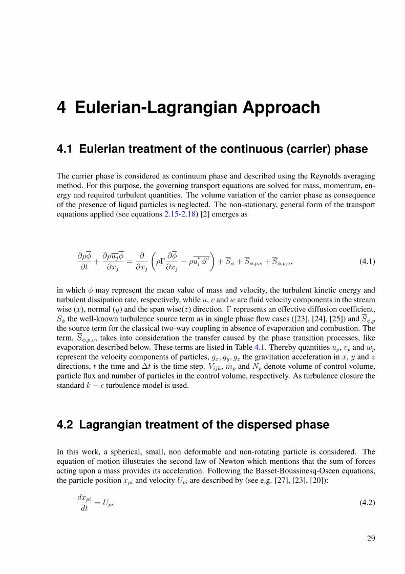
4 Eulerian-Lagrangian Approach
4.1 Eulerian treatment of the continuous (carrier) phase
The carrier phase is considered as continuum phase and described using the Reynolds averagingmethod. For this purpose, the governing transport equations are solved for mass, momentum, en-ergy and required turbulent quantities. The volume variation of the carrier phase as consequenceof the presence of liquid particles is neglected. The non-stationary, general form of the transportequations applied (see equations 2.15-2.18) [2] emerges as
∂ρφ
∂t+∂ρujφ
∂xj=
∂
∂xj
(ρΓ
∂φ
∂xj− ρu′′
i φ′′
)+ Sφ + Sφ,p,s + Sφ,p,v, (4.1)
in which φ may represent the mean value of mass and velocity, the turbulent kinetic energy andturbulent dissipation rate, respectively, while u, v andw are fluid velocity components in the streamwise (x), normal (y) and the span wise(z) direction. Γ represents an effective diffusion coefficient,Sφ the well-known turbulence source term as in single phase flow cases ([23], [24], [25]) and Sφ,pthe source term for the classical two-way coupling in absence of evaporation and combustion. Theterm, Sφ,p,v, takes into consideration the transfer caused by the phase transition processes, likeevaporation described below. These terms are listed in Table 4.1. Thereby quantities up, vp and wprepresent the velocity components of particles, gx, gy, gz the gravitation acceleration in x, y and zdirections, t the time and ∆t is the time step. Vijk, mp and Np denote volume of control volume,particle flux and number of particles in the control volume, respectively. As turbulence closure thestandard k − ε turbulence model is used.
4.2 Lagrangian treatment of the dispersed phase
In this work, a spherical, small, non deformable and non-rotating particle is considered. Theequation of motion illustrates the second law of Newton which mentions that the sum of forcesacting upon a mass provides its acceleration. Following the Basset-Boussinesq-Oseen equations,the particle position xpi and velocity Upi are described by (see e.g. [27], [23], [20]):
dxpidt
= Upi (4.2)
29
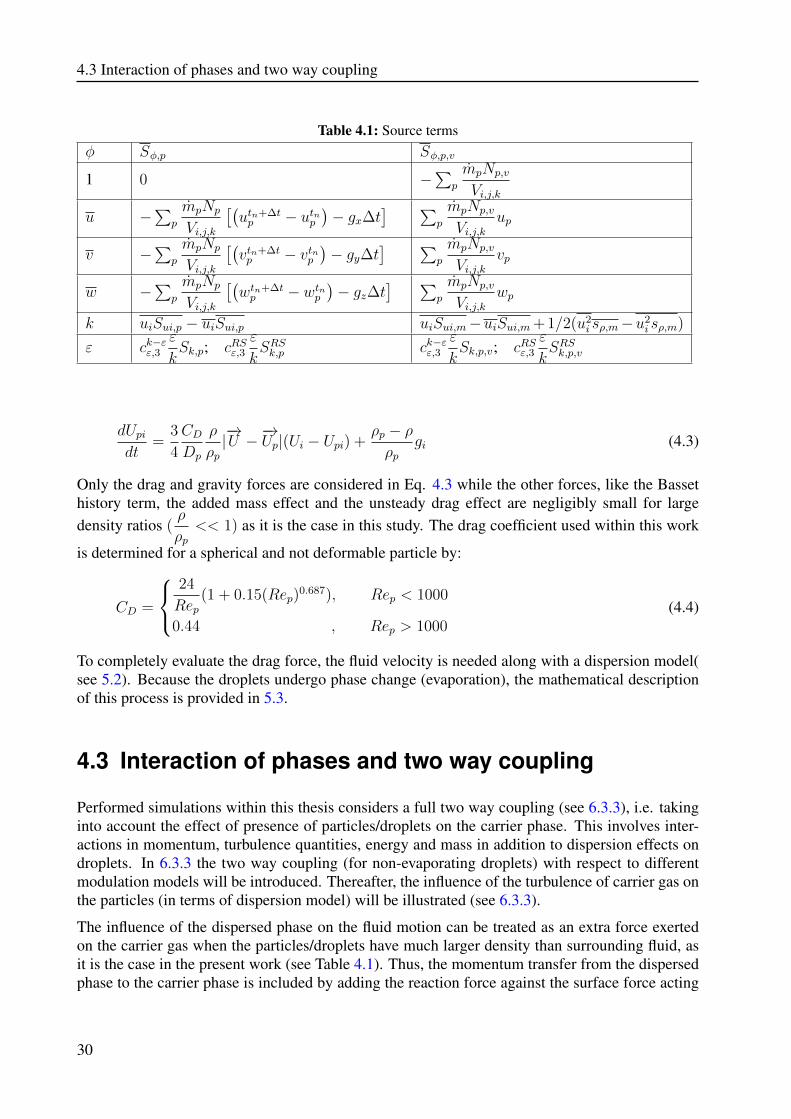
4.3 Interaction of phases and two way coupling
Table 4.1: Source termsφ Sφ,p Sφ,p,v
1 0 −∑
p
mpNp,v
Vi,j,k
u −∑
p
mpNp
Vi,j,k
[(utn+∆tp − utnp
)− gx∆t
] ∑p
mpNp,v
Vi,j,kup
v −∑
p
mpNp
Vi,j,k
[(vtn+∆tp − vtnp
)− gy∆t
] ∑p
mpNp,v
Vi,j,kvp
w −∑
p
mpNp
Vi,j,k
[(wtn+∆tp − wtnp
)− gz∆t
] ∑p
mpNp,v
Vi,j,kwp
k uiSui,p − uiSui,p uiSui,m−uiSui,m+ 1/2(u2i sρ,m−u2
i sρ,m)
ε ck−εε,3
ε
kSk,p; cRSε,3
ε
kSRSk,p ck−εε,3
ε
kSk,p,v; cRSε,3
ε
kSRSk,p,v
dUpidt
=3
4
CDDp
ρ
ρp|−→U −
−→Up|(Ui − Upi) +
ρp − ρρp
gi (4.3)
Only the drag and gravity forces are considered in Eq. 4.3 while the other forces, like the Bassethistory term, the added mass effect and the unsteady drag effect are negligibly small for largedensity ratios (
ρ
ρp<< 1) as it is the case in this study. The drag coefficient used within this work
is determined for a spherical and not deformable particle by:
CD =
24
Rep(1 + 0.15(Rep)
0.687), Rep < 1000
0.44 , Rep > 1000(4.4)
To completely evaluate the drag force, the fluid velocity is needed along with a dispersion model(see 5.2). Because the droplets undergo phase change (evaporation), the mathematical descriptionof this process is provided in 5.3.
4.3 Interaction of phases and two way coupling
Performed simulations within this thesis considers a full two way coupling (see 6.3.3), i.e. takinginto account the effect of presence of particles/droplets on the carrier phase. This involves inter-actions in momentum, turbulence quantities, energy and mass in addition to dispersion effects ondroplets. In 6.3.3 the two way coupling (for non-evaporating droplets) with respect to differentmodulation models will be introduced. Thereafter, the influence of the turbulence of carrier gas onthe particles (in terms of dispersion model) will be illustrated (see 6.3.3).
The influence of the dispersed phase on the fluid motion can be treated as an extra force exertedon the carrier gas when the particles/droplets have much larger density than surrounding fluid, asit is the case in the present work (see Table 4.1). Thus, the momentum transfer from the dispersedphase to the carrier phase is included by adding the reaction force against the surface force acting
30
4 Eulerian-Lagrangian Approach
on the particle/droplet to the Navier-Stokes equation 4.1. This model is known as force couplingmodel or particle-source-in-cell (PSI-Cell) model proposed by Crowe et al. [87]. To read moreabout two-way coupling, see 6.3.3.
31

5 Two-phase system andmicroprocesses under investigation
Turbulent spray systems are especially investigated in this work. The study includes physical phe-nomena of atomization (secondary breakup) along with droplet-droplet interactions, phase changeprocess, especially the droplet evaporation and the full two-way coupling between phases (disper-sion, modulation, etc.)
5.1 Atomization
In the sense of a broader definition, breakup includes the process when bulk liquid disintegratesinto droplets under the effect of the acting internal and external forces and also the process whenan existing droplet disintegrates into at least two, smaller droplets, or emits a larger number ofsignificantly smaller droplets. Based on this distinction, the entire breakup process can be split upinto two basic parts: the primary and secondary breakup, as discussed below.
5.1.1 Primary breakup
When a liquid emerges from a plain-orifice atomizer, such as a diesel injector nozzle, and theinjection velocity and the level of cavitation does not exceed a certain level, it has a continuumbody of cylindrical form. The various internal and external forces competing on the surface ofthis liquid column create oscillations and perturbations of the surface [124]. If these oscillationsand perturbations are amplified to a critical extent, the liquid body disintegrates into droplets.This process is referred to as primary breakup, and is very important because with initiating theatomization process and determining the extent of the liquid core, it provides the initial conditionsfor the dispersed flow region.
Depending on the physical conditions, this process can be diverse in nature, exhibiting substan-tially different characteristics. The categorization of these breakup types can be based on variousconsiderations. However, a fundamental platform is provided by the three most important physicalparameters related to spray breakup:
1. The Reynolds number as representing ratio of inertial forces to viscous forces, it is definedas displayed in 5.1 [124] [111]:
Re =uρlD
µl(5.1)
33
5.1 Atomization
2. The Weber number represents the ratio of aerodynamic force to the force of surface tension,and can be defined in two ways, depending on the physical mechanisms that are aimed to bedescribed [111]
Weg =u2ρgD
σ(5.2)
Wel =u2ρlD
σ(5.3)
In experimental analysis there is some degree of freedom in choosing the Weber number,since experimental researchers use it to describe their results with minimum number of pa-rameters. The choice might depend on type of the experiment, but e.g. for experimentswithout density variation liquid as well as gas Weber number could be chosen. The occur-rence and type of breakup can be very well related to the gas Weber number valid for thedroplet in consideration. Hence a lot of numerical models use this characteristic to switchfrom one model mechanism to another.
3. The third relevant number is the Ohnesorge number, also often referred to as the Laplacenumber, the viscosity number or the Z number, representing the ratio of liquid viscous forcesto surface tension forces. It is defined as [59]:
Oh =
√WelRe
=µl√σDρl
(5.4)
If the Ohnesorge number is used to account for the viscous forces during breakup in general,the assumption has to be made that the viscosity of surrounding gas is small compared tothat of the liquid, since the Ohnesorge number involves droplet properties only.
5.1.2 Secondary breakup
In the traditional approach for spray computation, the Eulerian equations for gaseous phase aresolved along with a Lagrangian model for droplet transport with two-way coupling of mass, mo-mentum, and energy exchange between the two phases [88]. The standard approach is to firstperform spray patternation studies for the injector used in combustion chambers and measure thesize distributions at various cross-sections from the injector. These distributions at the nearest po-sition to the nozzle are then used as an input to a numerical simulation which then computes thesecondary atomization of the injected droplets. The secondary atomization is typically modeledby standard deterministic breakup models based on Taylor Analogy Breakup (TAB) [89], or wave[90] models. However, this requires performance of experimental tests for any new injector designwhich can be very costly.
Liquid ’blobs’ with the size of the injector diameter are introduced and undergo atomization basedon the balance between aerodynamic and surface tension forces acting on the liquid phase.
34
5 Two-phase system and microprocesses under investigation
In the TAB model [89], oscillations of the parent droplet are modeled in the framework of a springmass system and breakup occurs when the oscillations exceed a critical value. In the wave model,new droplets are formed based on the growth rate of the fastest wave instability on the surface ofthe parent blob [90]. Both models are deterministic with ’single-scale’ production of new droplets.
In many combustion applications, however, injection of liquid jet takes place at high relative ve-locity between the two phases (high initial Weber number). Under these conditions, intriguingprocesses such as turbulence-induced breakup [52], multiple droplet collision in the dense spray re-gion [92], fluctuations due to cavitating flow inside the injector [93], etc., contribute to the processof atomization. At each spray location, this may result in droplet formation over a large spectrumof droplet-sizes and is not captured by the above models. In order to improve the TAB model, anenhanced TAB model (ETAB), where the product droplet size was obtained via a breakup cascademodeled by an exponential law, was proposed [94]. The parameters of this distribution functionwere derived from experimental data to achieve better performance of the model.
To predict the essential global features of these complex phenomena, a stochastic approach fordroplet breakup taking into account a range of product-droplet sizes is imperative (Gorokhovski,2001 [104]). The process of air-blast breakup can be considered in the framework of cascadeof a uncorrelated breakage events in series, independently from the initial distribution of sizes.Such a stochastic modeling of droplets production under these hypotheses down to the critical (ormaximum stable) size is followed in this work.
The cascade idea of breakup comes from the early work of Kolmogorov written in 1941 [55].in his work, Kolmogorov described the breakup of solid particles as a discrete random process,where the probability to break each parent particle on a given number of parts is independentof the parent particle size. From Lyapunov’s theorem, Kolmogorov has pointed out that such ageneral assumption leads to the log-normal distribution of particle size in the long-time limit. Inthis paper, the Kolmogorov’s discrete model has been reproduced in the form of evolution equationfor distribution function. The asymptotic solution of this equation has been applied to simulate thedrop breakup alongside with Lagrangian model of spray dynamics.
5.1.2.1 Kolmogorov’s (1941) Theory of the Particle Breakup
Following Kolmogorov [55] let us consider an ensemble of breaking solid particles at discretetime moments t = 0, 1, 2, .... These time moments are scaled by the breakup frequency ν ( t = νt). According to Komogorov [95], the number of particles N(r, t) of size ρ ≤ r was selectedamongst all particles N(t) at a given moment t. The expectations of total number of particlesand of particles of size ρ ≤ r were denoted as N(t) and N(r, t) correspondingly. Considering anoutcome of breakup per unit time [t, t + 1] of a given parent particle of size r, the mean numberQ(α) of secondary particles of size ρ ≤ αr(0 ≤ α1) was introduced. According to hypotheses ofKolmogorov, the probability to break each parent particle on a given number of parts is independentof the parent particle size. In other words, Q(α) does not depend of prehistory of breakup and isnot influenced by others parent particles. By this assumption, Kolmogorov writes:
N(r, t+ 1) =
∫ 1
0
(N(
r
α, t))dQ(α) (5.5)
35
5.1 Atomization
Introducing the logarithm of particle-size x = Inr, Kolmogorov pointed out that
T (x, t) =N(ex, t)
N(t)=N(ex, t)
N(t)(5.6)
Further, denoting ξ = Inα and Q(α) = Q(1)S(ξ), equation 5.5 is rewritten by Kolmogorov in thefollowing form:
T (x, t+ 1) =
∫ 0
∞T (x− ξ, t)dS(ξ) (5.7)
By Lyapunov’s theorem, Kolmogorov stated that from discrete model 5.7, the long-time limit formof T (x, t) tends to Gaussian function. Then the main result of Kolmogorov’s work is that N(r, t)is asymptotically governed by log-normal law.
The Asymptotic Differential Form of the Discrete Kolmogorov’s Model
Here the discrete model 5.7 is represented by its differential approximation in the long time limit.Using parabolic scaling of variables τ = ε2t, y = εx, where ε is a scaling parameter and t is scaledby breakup frequency, the equation 5.7 can be written as
T (y, τ + ε2) =
∫ 0
−∞T (y − εξ, τ)s(ξ)dξ (5.8)
Expanding both the left-hand side and the expression under integral in 5.8, one gets
T (y, τ + ε2) = T (y, τ) + ε2∂T (y, τ)
∂τ+O(ε4) (5.9)
T (y− ε2ξ, τ) = T (y, τ)− ε∂T (y, τ)
∂y+
1
2!(εξ)2∂
2T (y, τ)
∂y2+
1
3!(εξ)3∂
3T (y, τ)
∂y3+O(ε4) (5.10)
Substituting these expansions in 5.8 and coming back to variables t and x, one yields:
∂T (x, t)
∂t+O(ε4) = −〈ξ〉 ∂T (x, t)
∂x+
1
2!
⟨ξ2⟩ ∂2T (x, t)
∂x2+
1
3!
∂3T (x, t)
∂x3ε2∫ 0
−∞ξ3s(ξ)dξ+O(ε4)
(5.11)
36
5 Two-phase system and microprocesses under investigation
where 〈ξ〉 =∫ −∞
0ξs(ξ)dξ and 〈ξ2〉 =
∫ −∞0
ξ2s(ξ)dξ are two first moments of ξ. Assuming thatthe integral
∫ −∞0|lnα|2 dQ(α) is limited, the equation 5.11 can be written in the long-time limit
ε→ 0(t→∞), as
∂T (x, t)
∂t+ ν 〈ξ〉 ∂T (x, t)
∂x=
1
2!ν⟨ξ2⟩ ∂2T (x, t)
∂x2(5.12)
The dimensional time has been used in 5.12. The solution of 5.12 is Gaussian function. This re-peats the main result of Kolmogorov [95]. At the same time, an influence of the initial distributionbefore breakup starts can be taken into account by using 5.12. The solution of 5.12 verifies to be:
T (x, t) =
∫ 0
−∞
1√2π 〈ξ2〉νt
exp
[−(x− x0)2
2 〈ξ2〉 νt
]T0(x0 − 〈ξ〉 νt)dx0 (5.13)
where T0(x0) is the initial distribution of the logarithm of droplet radius and x0 is logarithm ofradius of the parent drop. One can rewrite equation 5.12 for the normalized distribution of radiusf(r):
∂f(r)
∂t= −ν 〈ξ〉 ∂
∂r(rf(r)) +
1
2ν⟨ξ2⟩ ∂∂r
(r∂
∂r(rf(r))
)(5.14)
The solution of this equation has the following form:
f(r, t) =1
r
∫ ∞0
1√2π 〈ξ2〉νt
exp
[−(ln r0
r+ 〈ξ〉 νt
)2
2 〈ξ2〉 νt
]f0(r0)dr0 (5.15)
where f0(r0) is the initial distribution of droplet radius before breakup starts.
5.1.2.2 Implementation into Computational Code
The modeling of the spray equation is often based on Lagrangian formulation [97]. The sprayis considered to be composed of discrete parcels of particles, each of which represents a groupof droplets of similar size, velocity and position. These groups of droplets are followed as theyinteract and exchange momentum and energy with surrounding gas. The basic ideas of this method,including the modeling of turbulent dispersion of particles, are presented in [98].
Here, the Lagrangian tracking is coupled with a stochastic computing of breakup as outlined in thefollowing. The product droplet velocity has been modeled and the breakup has been considereddown to the local magnitude of the critical (or maximum stable) radius, rcr. The liquid fuel wasinjected in the axial nozzle direction in form of discrete parcels of drops with characteristic sizeequal to the exit nozzle radius. The injection velocity was determined from the known liquidinjection rate.
37
5.1 Atomization
Let us consider the motion of a given j−th primary parcel that undergoes breakup. Before breakupstarts, the distribution function associated with this parcel is Dirac function at radius of the parentdrop. After passage of time, which is inversely the breakup frequency, the new droplets arise dueto breakup. In sequel, the droplet-radius distribution function changes. We suppose that the newdistribution may be described according to solution 5.15 taken at νt = 1 with 〈ξ〉 and 〈ξ2〉 asparameters of the model.
In order to alleviate computations, we can proceed in the following way. Let us assume that onceevery breakup time scale, all outcomes of breakup in the given parent parcel are in mean (overmany computations), recovered by one new parcel that replaces the parent one. The radius ofdroplet associated with produced parcel is sampled from 5.15. The new number of droplets iscomputed by mass conservation from the primary parcel to the secondary one. After the samplingprocedure, the current time, t, prescribed for produced parcel is counted from zero and Lagrangiantracking is continued up to the moment (νt = 1) of the further breakup. In computations, we usedexpressions obtained for the distribution of the logarithm of radius. The starting distribution forthe logarithm of droplet radius in j − th primary parcel is
T0j(x0) = δ(x0 − xj) (5.16)
Using this distribution function in 5.13 at νt = 1, one can express the solution by the error functionerf :
Tj(x, t) =1
2
[1 + erf
(x− xj − 〈ξ〉√
2 〈ξ2〉
)](5.17)
The product droplet velocity is computed by adding to the primary parcel velocity a velocity wbu,which is randomly distributed in a plane normal to the relative velocity vector between the parentdroplet and gas. The quantity of wbu is determined by the mean local Sauter radius of parent drops,r32, and the breakup frequency, ν:
wbu = r32ν (5.18)
How to determine ν will be shown in eq. 5.26.
5.1.2.3 Critical radius, breakup frequency
The critical (or maximum stable) radius is determined when disruptive hydrodynamic forces arebalanced by capillary forces:
rcr = Wecrδ/ρgu2r (5.19)
38
5 Two-phase system and microprocesses under investigation
where ur is the relative between liquid and gas velocity, δ is the surface tension coefficient, Wecris the critical Weber number, which can be taken of order one over a large interval of Ohnesorgenumbers [99], [59]. In the paper, written in 1949 [100], Kolmogorov considered the stretched dropof insoluble liquid that was submerged in a turbulent flow. Using the Obuchov- Kolmogorov’s scal-ing law for the velocity difference across a size when the surface tension force becomes significant,Kolmogorov introduced a critical size of produced droplets as:
rcr =1
2
(Wecrδ
ε2/3ρg
)3/5
if 2r >> η (5.20)
rcr =1
2
(Wecrδν
ερg
)1/3
if 2r >> η (5.21)
where ε is the mean viscous dissipation rate and ρg is density in the gas. An estimation of rcr byusing experimental data from [101] gives an enhanced magnitude of rcr comparing to the mea-surements. In order to account for the inertia of liquid, namely for the density of the liquid ρl theexpression 5.20 can be modified. Estimating the mean square of relative droplet-to-gas velocity bymean viscous dissipation and Stokes time scale [102],
⟨u2r
⟩= ετst (5.22)
one yields a new expression for critical radius:
rcr =361/3
2
(Wecrδν
ερl
)1/3
(5.23)
Using the experimental data from [101] water density, 1000kg/m3; gas viscosity, 1.5x10⁻⁵m2/s;gas orifice size, 2.1mm; surface tension, 0.07kg/s2; gas injection velocity, 140 m/s and by settingthe turbulent gas velocity at one tenth of the gas injection velocity, one gives for critical radius3x10−5 m, which is of the same order that was measured in [101]. At the same time, expressions5.23 requires a reliable knowledge of viscous dissipation rate, which is a problem in the turbu-lence computation. For these reasons, the critical radius is calculated in this work by the standardexpression 5.19, where ur = Vg − vp is calculated by the mean relative velocity between gas andliquid particle, computed by the model of turbulent of particles. Note that introducing the turbu-lent Weber number, Wetur = ρglturu
2tur/δ, and using 5.22, one may write for the critical Weber
number:
Wecr =1
36
ρlρgReturWetur
(2rcrltur
)3
(5.24)
39
5.1 Atomization
Assuming that at scales where breakup takes place Retur (turbulent reynold’s number) is of orderof unity and the turbulent length scale ltur ≈ η, one may propose:
2rcrη
= 3.3
(WeηWecr
)−1/3(ρgρl
)1/3
(5.25)
The choice of the breakup frequency has to be stated from the physics of atomization. In this work,the breakup time scale is
ν = B|vg − vp|r32
√ρgρl
(5.26)
where r32 is the local Sauter mean radius of parent drops and B = 1/√
3 is taken from the TABmodel [89].
5.1.2.4 Choice of parameters
Multiplying 5.14 by r and integrating over the entire r - range leads to an expression for the firstmoment
〈r〉 = 〈r〉t=0 exp⌊ν(〈ξ〉+ 0.5
⟨ξ2⟩)t⌋
(5.27)
The condition
〈ξ〉 < −1
2
⟨ξ2⟩
(5.28)
is provided for 〈r〉〈r〉t=0
. In this work, the magnitude for 〈ξ2〉 is supposed to be proportional to themaximal dispersion of radius 〈ξ2〉 ∝ ln1 − ln rcr
r32Replacing in 5.25 η by the local Sauter mean
diameter of parent drops, one may assume that
⟨ξ2⟩≈ −lnrcr
r32
≈ constln(Wer32
Wecr
)(5.29)
and 〈ξ〉 is an arbitrary parameter to be taken according to 5.28 and 5.29.
40
5 Two-phase system and microprocesses under investigation
5.2 Turbulent Dispersion
The Eulerian approach for the fluid flow gives the mean values of the fluid velocity componentsand the turbulent quantities. However, the particle experiences at its position the instantaneousfluid velocity −→u , which is stochastic. To account for the effect of this stochastic behavior of fluidflow on the particle, so called turbulent dispersion, a dispersion model is needed. Three dispersionmodels are used in this work to evaluate the instantaneous fluid velocity at the position of particle.They are (a) the particle Langevin model (PLM), (b) the isotropic Random Walk model (RWM-Iso)and (c) the anisotropic Random Walk model (RWM-Aniso).
5.2.1 Particle Langevin Model (PLM)
As pointed out above, this approach consists of generating directly the fluid velocities followingthe particle path by modeling the de-correlation induced by the mean and turbulent fluid-particlerelative motion. An elaborated presentation of PLM is introduced by Minier et al. (2001). Thefluid velocity fluctuation seen by particles emerges as follows:
dui = −uj∂U i
∂xjdt+
∂uiuj∂xj
dt+ (Upj − U j)∂U i
∂xjdt+
1
TLiHijuidt+Bijξi, (5.30)
where Ui and uiuj are the mean velocity and the Reynolds stress tensor. Furthermore, Hij is ageneralization of the drift matrix for arbitrary mean slip between the flow phases, Bij the diffusionmatrix and ξi a Gaussian random process. TLi represents the Lagrangian time scale and is definedas follows:
TLi =1(
1
2+
3
4C0
)ε
kbi
. (5.31)
In equation 5.31 ,C0 = 2.1 and bi are Csanady factors which are mostly used to estimate the dif-ference between the stream wise and the transversal time scales. bi is defined as below:
bi = b| + (b| − byx)(Upi − Ui)2∣∣∣−→Up −−→U ∣∣∣2 (5.32)
b| =
(1 + β2 |
−→Up −
−→U |2
2k/3
)0.5
, byx =
(1 + 4β2 |
−→Up −
−→U |2
2k/3
)0.5
(5.33)
β =TLTE
=1
CLis the ratio between the Lagrangian time and Eulerian time scales. In this work the
common value of CL = 1.1. is used (see Horender ).The matrix Hij is defined in the following form:
41
5.2 Turbulent Dispersion
Hij = byxδij + b|rirj, (5.34)
where ri is the unit vector in direction of the mean slip between fluid and particle.The diffusion term (Bij) is defined as:
(BBT )ij = Dij, (5.35)
where Dij has the following form:
Dij = ε
(C0λHij +
2
3(λHij − δij)
). (5.36)
Further, λ is given by:
λ =3tr(HijRij)
2ktr(Hij), (5.37)
where tr(.) and Rij denote the trace and the Reynolds stress tensor, respectively. Peirano et al.2005 suggested a Simplified Langevin Model which takes into account the drift between the inertialparticles and the fluid particles. The resulting equation for fluctuating velocity ui is as follows:
dui = −uj∂U i
∂xjdt+
∂uiuj∂xj
dt︸ ︷︷ ︸1
+ (Upj − U i)∂U i
∂xj︸ ︷︷ ︸2
(5.38)
− 1
TL,iuidt︸ ︷︷ ︸3
+
√√√√ε
((C0 +
2
3
)bik
k− 2
3
)dWi(t)︸ ︷︷ ︸
4
. (5.39)
The first term is a fluid drift term. It accounts for the change of the fluctuation due to the changesof the fluid flow. Note that the Reynolds stresses are calculated following the standardK−εmodelas follows:
Rij = −uiuj = νt
(∂U i
∂xj+∂U j
∂xi
)− 2
3kδij (5.40)
The second term accounts for the drift between the particle and the mean fluid velocity field. Thethird term considers the memory effects. It relates the new fluctuating fluid velocity to the previousby the Lagrangian time scale TL,i. The fourth term expresses the diffusion process by includingrandomness through the Wiener process dWi(t). The diffusion in different directions is assumed
42
5 Two-phase system and microprocesses under investigation
independent, but anisotropic Minier et al. 2001. k is a dimensionless turbulent kinetic energydefined by:
k =3
2
∑3i=1 biu
2i∑3
i=1 bi(5.41)
Note that henceforth the simplified version of Langevin equation will be referred as PLM and isused in the numerical simulations presented in this work.
5.2.2 Isotropic Random Walk Model (RWM-Iso)
In order to evaluate the capability of PLM, two simple models are considered for comparison. Thefirst is the Lagrangian stochastic approach using the fluid turbulent variables (Sommerfeld et. al.[25]) (2003), [39] (1996), Sadiki et al. (2005), Chrigui et al. (2004), Melheim et al. (2005),Walklate (1995)). It is obtained from the discretized equations for a Markov-chain random-walkof fluid particle velocity fluctuations for homogeneous isotropic turbulence as:
un+1,i = RP,i(∆t,∆r)un,i + σi
√1−R2
P,i(∆t,∆r)ξi(tn). (5.42)
Its solution for given initial conditions represents a Markov sequence of successive fluid particlevelocity at time interval of ∆t. Hence, this model can be seen as a Langevin model for an Orstein-Uhlenbeck process written in finite difference form. Hereafter it will be referred as isotropic Ran-dom Walk dispersion model (RWM-Iso).In Eq. 5.42, ξi(tn) denotes a Gaussian random variable at time step tn. ∆r represents the spatialdisplacements during the time interval ∆t and
RP,i(∆t,∆r) = RL,i(∆t) ∗RE,i(∆r) (5.43)
is a typical correlation used to compute the fluctuation of the fluid element ui at the particle lo-cation. Thereby, the evolution of the fluid element velocity fluctuation along the stream line isdetermined using the Lagrangian correlation factorRL,i(∆t), while the fluid element velocity fluc-tuation located at the particle position is correlated with the fluid element location using the Eu-lerian correlation factor RE,i(∆r). They are expressed in Sommerfeld et. al. [25]) (2003), [39](1996), Chrigui et al. (2004), Chrigui et al. (2010), Sadiki et al. (2005), Melheim et al. (2005)as:
RL,i(∆t) = exp(− dt
TLi) (5.44)
RE,i(∆t) = (f(∆r)− g(∆r))∆ri∆rj
∆r2+ (∆r)gδij, (5.45)
43
5.3 Evaporation
respectively. The quantity TL,i represents the Lagrangian integral time scale (see Eq. 5.32) cal-culated in the framework of k − ε turbulence model according to TL,i = cTk/ε = cTσ
2/ε withcT = 0.3 and σ2 = k. The longitudinal and transversal correlation functions f(∆r) and g(∆r) inEq. 5.45 are computed using the following expressions:
f(∆r) = exp(−∆r
LE); g(∆r) = (1− ∆r
2LE)exp(−∆r
LE) (5.46)
where LE = c′LTLσ (with c′L = 0.3) represents the turbulent length scale.
5.2.3 Anisotropic Random Walk Model (RWM-Aniso)
To account for flow anisotropy and drift correction Legg & Raupach [50] extended the isotropicformulation of RWM-Iso by including an additional term, which is derived from the momentumequation (see Eq. 5.47). This term should consider the anisotropy of the flow and avoid non-physical behavior, such as the accumulation of particles in regions of low velocity variance. Eq.5.42 then reads:
un+1,i = RP,i(∆t,∆r)un,i + σi√
1−R2P,i(∆t,∆r)ξi(tn)
+(1−RP,i(∆t,∆r))TL,i∂uiui∂xi
(5.47)
It should here be noted that this model has been derived for a stationary, horizontally homogeneousflow over a flat plate. Therefore, it does not have the capability to deal properly with the threedimensionality nature of turbulence in complex flows.
5.3 Evaporation
In many devices, as it is in cases investigated in this work, fuels are sprayed as fine droplets intoa combustion chamber. The droplets undergo evaporation, so that the evaporation represents adecisive process of the fuel preparation in such devices. Numerous theoretical studies literaturehave been carried out for the description of droplet evaporation. In the most general case the dropletevaporation process includes two main phases: (1) detachment of fuel molecules from the surfaceof the droplet into gas in the immediate vicinity of droplets (evaporation proper) and (2) diffusionof fuel vapor from the surface of the droplet into the ambient gas. The mathematical modelingof the first process is far more complicated than the modeling of the second process. Hence, inmost practical application, the researchers tried to focus just on the second process, ignoring thedetails of the first. The models, which they used were based on the assumption that fuel vaporin the vicinity of the droplet surface is always saturated. Hence, the rate of fuel evaporation isequal to the rate of fuel diffusion from the droplet surface to ambient gas. These are known as thehydrodynamic models of droplet evaporation. In contrast to these, models taking into account thedetails of detachment of fuel molecules are known as kinetic models (if they are based on modeling
44
5 Two-phase system and microprocesses under investigation
of the dynamics of individual molecules).Empirical correlations also exist, which are not directly linked with any physical evaporation modelIn this section the evaporation model, the so-called uniform temperature model by Abramson andSirignano [109] used in the frame of this thesis, will be introduced.
5.3.1 Abramzon and Sirignano model: Uniform temperature model
This model represents an equilibrium evaporation model based on the film thickness theory. Ac-cordingly, two time scales characterizing the turbulence and the thermodynamics of the vapor-ization will be introduced along with a new dimensionless number to characterize the turbulencedroplet vaporization interaction regimes. In order to ensure a mathematical description, one shouldreduce the complexity of the theoretical description. Thus the following basic assumptions andsimplifications are made according to [42]:
1. One component model is considered, so that one solely deals with the so-called infiniteconductivity model.
2. Droplets are assumed to be spherical.
3. Secondary atomization and coalescence of droplets are neglected as the evaporation processis only accounted for in the we concentrate on the dilute spray region. In other words simpleelastic collisions between droplets and wall are assumed without any kind of film formation[148].
4. The influence of the surface tension is neglected and assume a uniform pressure around thedroplet is assumed.
5. Uniform physical properties of the surrounding fluid and liquid-vapor thermal equilibriumon the droplet surface are assumed.
6. The ambient air is not soluble in the droplet fluid.
7. Chemical reactions and radiation are not considered.
In order to further simplify the modeling of the evaporation process, the evaporation process issubdivided into three spatial zones (Figure 5.1):
1. The ambient gas phase, which represents the region infinitely far from the droplet. Thetemperature and vapor concentration are those of the carrier phase.
2. The droplet interior
3. The liquid/gas interface, which represents the region governing transport processes. In thisregion one observes radial mass diffusion, heat convection and conduction as well as forcedconvection.
The transport processes linked to the forced convection from the gas flow around the droplet,(located at the liquid/gas interface as presented above), is the fundamental difficulty in the devel-opment of practical evaporation models. For solving this problem, one has to start from an isolateddroplet in a stagnant gas atmosphere with spherical symmetric transport of mass and energy. Theeffect of forced convection is then taken into account by means of empirical correlation factors(modified Nusselt and Sherwood numbers), as they will be introduced later on.
45
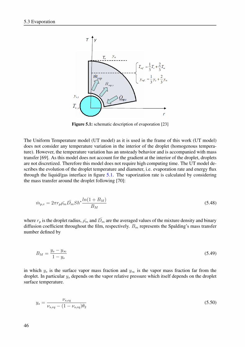
5.3 Evaporation
Figure 5.1: schematic description of evaporation [23]
The Uniform Temperature model (UT model) as it is used in the frame of this work (UT model)does not consider any temperature variation in the interior of the droplet (homogenous tempera-ture). However, the temperature variation has an unsteady behavior and is accompanied with masstransfer [69]. As this model does not account for the gradient at the interior of the droplet, dropletsare not discretized. Therefore this model does not require high computing time. The UT model de-scribes the evolution of the droplet temperature and diameter, i.e. evaporation rate and energy fluxthrough the liquid/gas interface in figure 5.1. The vaporization rate is calculated by consideringthe mass transfer around the droplet following [70]:
mp,v = 2πrpρmDmSh∗ ln(1 +BM)
BM
(5.48)
where rp is the droplet radius, ρm and Dm are the averaged values of the mixture density and binarydiffusion coefficient throughout the film, respectively. Bm represents the Spalding’s mass transfernumber defined by
BM =ys − y∞1− ys
(5.49)
in which ys is the surface vapor mass fraction and y∞ is the vapor mass fraction far from thedroplet. In particular ys depends on the vapor relative pressure which itself depends on the dropletsurface temperature.
ys =νs,eq
νs,eq − (1− νs,eq)θ2
(5.50)
46
5 Two-phase system and microprocesses under investigation
where θ2 is the ratio of molecular weights. The molar mass fraction νs,eq is related to the saturationpressure through the Clausius-Clapeyron equation. Therefore it is referred to as an equilibriumbased model. The accuracy of the evaporation rate depends strongly on the determination of thevalues of ,ρm and Dm . Physical properties of the air vapor mixture (in the gaseous film aroundthe droplet) are determined using the reference temperature and mass fraction. They are calculatedusing the Simpson or Sparrow & Gregg ’1/3’ rule [71], from which the best accuracy of thesequantities have been obtained ( see 5.1). The droplet radius is obtained from the equation of thediameter evolution for each droplet by:
dDp
dt= − 2mp,v
πρLD2p
− Dp
3ρL
∂ρL∂Tp
dTpdt, (5.51)
where ρL is the liquid density, Dp the droplet diameter and Tp the droplet temperature. Effectsof convection on the vaporization and the heat flux rate are taken into account by means of semi-empirical correlations such as those for the drag coefficient, the Sherwood number and the Nusseltnumber. The quantity Sh∗ denotes the modified Sherwood number which includes the effects ofthe Stefan flow. It is defined by
Sh∗ = 2 +Sho − 2
FM(5.52)
where
Sh0 = 1 + (1 +RepScp)1/3f(Rep) (5.53)
Sh0 accounts for the bulk convection of a non-evaporating spherical droplet. Rep is the dropletReynolds number and Scp is the Schmidt number while f(Rep) is an empirical function defined asf(Rep) = Re0.77
p and FM is a correction factor, which takes into consideration the relative changeof the mass film thickness due to the droplet evaporation process:
FM = FM(BM) = (1 +BM)0.7ln(1 +BM)
BM
(5.54)
The evaporation is coupled with the droplet energy/heating in 5.51 where the droplet temperaturevariation is described by
dTpdt
= − 6Ql
ρπcpLD3p
, (5.55)
47
5.3 Evaporation
where cpL denotes the heat capacity coefficient of the liquid and Ql the heat flux rate penetratinginto the droplet. The latter is calculated similarly to the evaporation rate and related to it by:
Ql = mp,v
[cpm(T∞ − Tp)
BT
− hv(Tp)], (5.56)
where hv(Tp) = r(Tp)+Ql/mp,v expresses the effective latent heat of vaporization. It is a functionof temperature and varies with the considered liquid. r(Tp) is the true latent heat of vaporizationand BT is the Spalding heat transfer number expressed by
BT =¯cp,v(T∞ − Tp)
r(Tp) + Ql/mp,v
, (5.57)
It is related to the mass transfer number BM by
BM = (1 +BM)φ − 1, (5.58)
where
φ =cp,vcp,m
Sh∗
Nu∗1
Le. (5.59)
The variable φ depends on the thermo-physical properties, the Lewis number Le and the modifiedSherwood and Nusselt numbers (Sh∗ and Nu∗). The modified Nusselt number in 5.59 is definedby:
Nu∗ = 2 +Nu0 − 2
FT, (5.60)
where
Nu0 = 1 + (1 +RepPr)1/3f(Rep). (5.61)
Nu0 expresses the Nusselt number for a non-evaporating spherical droplet with f(Rep) as definedabove. Pr is the Prandtl number and FT is a correction factor which accounts for the change ofthe temperature within the film thickness due to the droplet evaporation process:
FT = FT (BT ) = (1 +BT )0.7ln(1 +BT )
BT
. (5.62)
48
5 Two-phase system and microprocesses under investigation
In 5.59 cpv and cpm are the heat capacity coefficients of vapor and mixture, respectively. BetweenNu0 and the modified Nusselt numbers Nu∗ the relationship 5.61 is considered. No correctionto the drag coefficient due to the evaporation process has been taken into consideration. The gasviscosity in the droplet Reynolds number near the droplet has been estimated at a well-definedreference state of temperature and vapor mass fraction according to the averaging ’1/3 rule’ [107].
49

6 Numerical procedure
The development and analysis of discretization methods for systems of ordinary and partial dif-ferential equations and the implementation of the respective algorithms in computer codes are theonly way to transform the theoretical work into practical one which can provide useable results.The challenge is then shifted from the continuous mathematics to discrete mathematics. This sec-tion deals with the used numerical procedure to discretize the governing equations for the carrierphase, the dispersed phase and the coupling method between both phases. The statistical methodfor properties sampling and the convergence criteria will be also introduced later.
6.1 Solution procedure of the transport equations for thecontinuous phase
Following Ferziger and Peri [72], a numerical solution method includes a mathematical model, adiscretization method, a coordinate and basis vector system, a numerical grid, a finite approxima-tion and a solution method. In this work the CFD package FASTEST-3D (Flow Analysis SolvingTransport Equations Simulating Turbulence 3 Dimensional) is used. The program was originallydeveloped by INVENT Computing GmbH (Erlangen, Germany) and obtained as a source codein the framework of the Collaborative Research Project SFB-568. Consequently, the parts of nu-merical solution method mentioned above and applied in the present work are those based on thefeatures of FASTEST-3D:
1. Finite volume discretization method (FVM) based on hexahedral control volumes;
2. Cartesian coordinate and basis vector system;
3. Boundary-fitted non-orthogonal block-structured grid with matching interfaces and collo-cated variable arrangement;
4. Implicit and semi-implicit temporal and first and second order spatial discretization schemes;
5. Strongly implicit procedure for the solution (iterative) of the linearised equation system;
6. Full geometrical multigrid solver for the acceleration of convergence;
7. Parallelization based on domain decomposition in space using the MPI message passinglibrary.
Important details as well as implementation of the boundary conditions will be presented anddiscussed in the following sections.
51
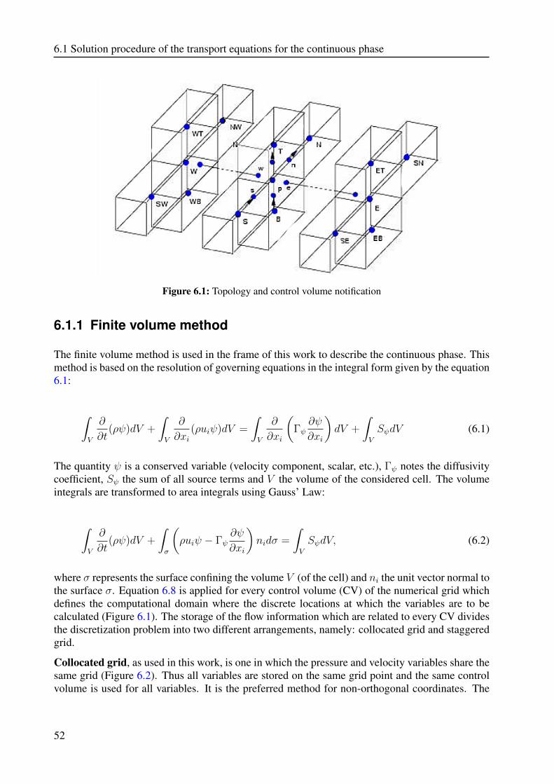
6.1 Solution procedure of the transport equations for the continuous phase
Figure 6.1: Topology and control volume notification
6.1.1 Finite volume method
The finite volume method is used in the frame of this work to describe the continuous phase. Thismethod is based on the resolution of governing equations in the integral form given by the equation6.1:
∫V
∂
∂t(ρψ)dV +
∫V
∂
∂xi(ρuiψ)dV =
∫V
∂
∂xi
(Γψ
∂ψ
∂xi
)dV +
∫V
SψdV (6.1)
The quantity ψ is a conserved variable (velocity component, scalar, etc.), Γψ notes the diffusivitycoefficient, Sψ the sum of all source terms and V the volume of the considered cell. The volumeintegrals are transformed to area integrals using Gauss’ Law:
∫V
∂
∂t(ρψ)dV +
∫σ
(ρuiψ − Γψ
∂ψ
∂xi
)nidσ =
∫V
SψdV, (6.2)
where σ represents the surface confining the volume V (of the cell) and ni the unit vector normal tothe surface σ. Equation 6.8 is applied for every control volume (CV) of the numerical grid whichdefines the computational domain where the discrete locations at which the variables are to becalculated (Figure 6.1). The storage of the flow information which are related to every CV dividesthe discretization problem into two different arrangements, namely: collocated grid and staggeredgrid.
Collocated grid, as used in this work, is one in which the pressure and velocity variables share thesame grid (Figure 6.2). Thus all variables are stored on the same grid point and the same controlvolume is used for all variables. It is the preferred method for non-orthogonal coordinates. The
52
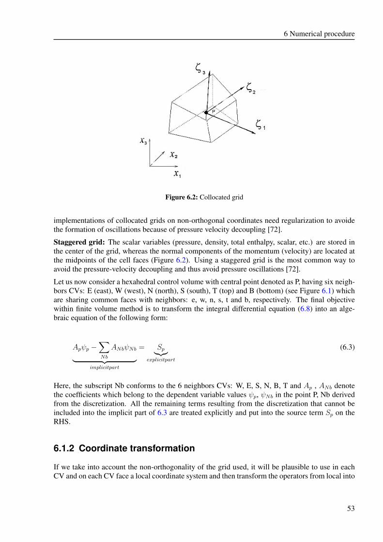
6 Numerical procedure
Figure 6.2: Collocated grid
implementations of collocated grids on non-orthogonal coordinates need regularization to avoidethe formation of oscillations because of pressure velocity decoupling [72].
Staggered grid: The scalar variables (pressure, density, total enthalpy, scalar, etc.) are stored inthe center of the grid, whereas the normal components of the momentum (velocity) are located atthe midpoints of the cell faces (Figure 6.2). Using a staggered grid is the most common way toavoid the pressure-velocity decoupling and thus avoid pressure oscillations [72].
Let us now consider a hexahedral control volume with central point denoted as P, having six neigh-bors CVs: E (east), W (west), N (north), S (south), T (top) and B (bottom) (see Figure 6.1) whichare sharing common faces with neighbors: e, w, n, s, t and b, respectively. The final objectivewithin finite volume method is to transform the integral differential equation (6.8) into an alge-braic equation of the following form:
Apψp −∑Nb
ANbψNb︸ ︷︷ ︸implicitpart
= Sp︸︷︷︸explicitpart
(6.3)
Here, the subscript Nb conforms to the 6 neighbors CVs: W, E, S, N, B, T and Ap , ANb denotethe coefficients which belong to the dependent variable values ψp, ψNb in the point P, Nb derivedfrom the discretization. All the remaining terms resulting from the discretization that cannot beincluded into the implicit part of 6.3 are treated explicitly and put into the source term Sp on theRHS.
6.1.2 Coordinate transformation
If we take into account the non-orthogonality of the grid used, it will be plausible to use in eachCV and on each CV face a local coordinate system and then transform the operators from local into
53
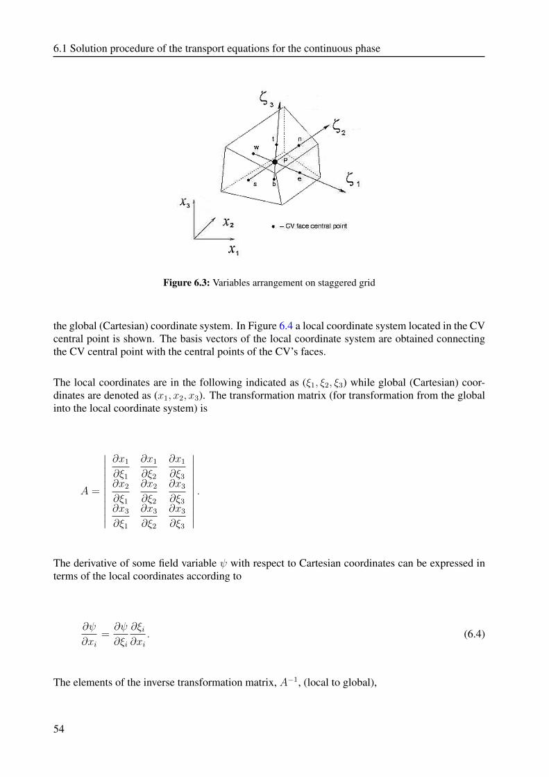
6.1 Solution procedure of the transport equations for the continuous phase
Figure 6.3: Variables arrangement on staggered grid
the global (Cartesian) coordinate system. In Figure 6.4 a local coordinate system located in the CVcentral point is shown. The basis vectors of the local coordinate system are obtained connectingthe CV central point with the central points of the CV’s faces.
The local coordinates are in the following indicated as (ξ1, ξ2, ξ3) while global (Cartesian) coor-dinates are denoted as (x1, x2, x3). The transformation matrix (for transformation from the globalinto the local coordinate system) is
A =
∣∣∣∣∣∣∣∣∣∣∣
∂x1
∂ξ1
∂x1
∂ξ2
∂x1
∂ξ3∂x2
∂ξ1
∂x2
∂ξ2
∂x3
∂ξ3∂x3
∂ξ1
∂x3
∂ξ2
∂x3
∂ξ3
∣∣∣∣∣∣∣∣∣∣∣.
The derivative of some field variable ψ with respect to Cartesian coordinates can be expressed interms of the local coordinates according to
∂ψ
∂xi=∂ψ
∂ξi
∂ξi∂xi
. (6.4)
The elements of the inverse transformation matrix, A−1, (local to global),
54
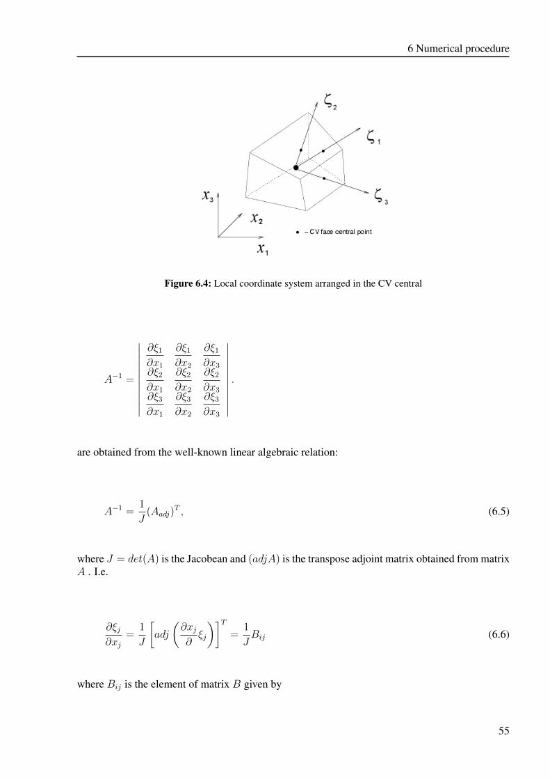
6 Numerical procedure
Figure 6.4: Local coordinate system arranged in the CV central
A−1 =
∣∣∣∣∣∣∣∣∣∣∣
∂ξ1
∂x1
∂ξ1
∂x2
∂ξ1
∂x3∂ξ2
∂x1
∂ξ2
∂x2
∂ξ2
∂x3∂ξ3
∂x1
∂ξ3
∂x2
∂ξ3
∂x3
∣∣∣∣∣∣∣∣∣∣∣.
are obtained from the well-known linear algebraic relation:
A−1 =1
J(Aadj)
T , (6.5)
where J = det(A) is the Jacobean and (adjA) is the transpose adjoint matrix obtained from matrixA . I.e.
∂ξj∂xj
=1
J
[adj
(∂xj∂ξj
)]T=
1
JBij (6.6)
where Bij is the element of matrix B given by
55
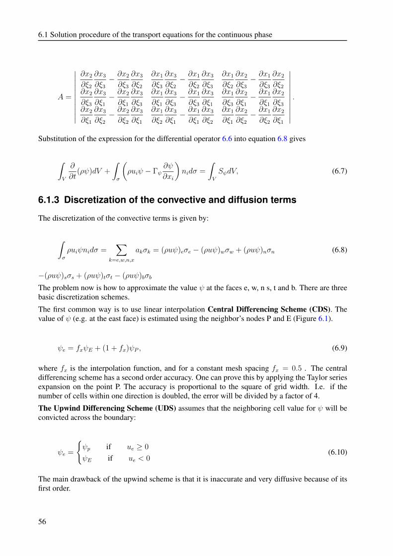
6.1 Solution procedure of the transport equations for the continuous phase
A =
∣∣∣∣∣∣∣∣∣∣∣
∂x2
∂ξ2
∂x3
∂ξ3
− ∂x2
∂ξ3
∂x3
∂ξ2
∂x1
∂ξ3
∂x3
∂ξ2
− ∂x1
∂ξ2
∂x3
∂ξ3
∂x1
∂ξ2
∂x2
∂ξ3
− ∂x1
∂ξ3
∂x2
∂ξ2∂x2
∂ξ3
∂x3
∂ξ1
− ∂x2
∂ξ1
∂x3
∂ξ3
∂x1
∂ξ1
∂x3
∂ξ3
− ∂x1
∂ξ3
∂x3
∂ξ1
∂x1
∂ξ3
∂x2
∂ξ1
− ∂x1
∂ξ1
∂x2
∂ξ3∂x2
∂ξ1
∂x3
∂ξ2
− ∂x2
∂ξ2
∂x3
∂ξ1
∂x1
∂ξ2
∂x3
∂ξ1
− ∂x1
∂ξ1
∂x3
∂ξ2
∂x1
∂ξ1
∂x2
∂ξ2
− ∂x1
∂ξ2
∂x2
∂ξ1
∣∣∣∣∣∣∣∣∣∣∣.
Substitution of the expression for the differential operator 6.6 into equation 6.8 gives
∫V
∂
∂t(ρψ)dV +
∫σ
(ρuiψ − Γψ
∂ψ
∂xi
)nidσ =
∫V
SψdV, (6.7)
6.1.3 Discretization of the convective and diffusion terms
The discretization of the convective terms is given by:
∫σ
ρuiψnidσ =∑
k=e,w,n,x
akσk = (ρuψ)eσe − (ρuψ)wσw + (ρuψ)nσn (6.8)
−(ρuψ)sσs + (ρuψ)tσt − (ρuψ)bσb
The problem now is how to approximate the value ψ at the faces e, w, n s, t and b. There are threebasic discretization schemes.
The first common way is to use linear interpolation Central Differencing Scheme (CDS). Thevalue of ψ (e.g. at the east face) is estimated using the neighbor’s nodes P and E (Figure 6.1).
ψe = fxψE + (1 + fx)ψP , (6.9)
where fx is the interpolation function, and for a constant mesh spacing fx = 0.5 . The centraldifferencing scheme has a second order accuracy. One can prove this by applying the Taylor seriesexpansion on the point P. The accuracy is proportional to the square of grid width. I.e. if thenumber of cells within one direction is doubled, the error will be divided by a factor of 4.
The Upwind Differencing Scheme (UDS) assumes that the neighboring cell value for ψ will beconvicted across the boundary:
ψe =
{ψp if ue ≥ 0
ψE if ue < 0(6.10)
The main drawback of the upwind scheme is that it is inaccurate and very diffusive because of itsfirst order.
56
6 Numerical procedure
The Flux Blending switches between the two, according to the relative size of the convective anddiffusive fluxes across the cell face. By resulting in oscillation, one can combine UDC and CDSto calculate the value at the faces e:
ψe = ψUDSe︸ ︷︷ ︸I
+ γ(ψCDSe − ψCDSe )︸ ︷︷ ︸II
, (6.11)
where 0 ≤ γ ≤ 1 is a factor which scales the manner of flux blending. For γ = 1, the interpolationis pure CDS whereas for γ = 1, the interpolation is pure Upwind. Part I of 6.11 is treated implicitlywhereas part II is treated explicitly. The flux blending scheme is a good control tool to achievean optimum between stability and accuracy. For the diffusive part, a centered difference for thediscretization of the normal gradient of the flux on the control volumes faces is used. Thus thediffusive part is discretized by:
(∂ψ
∂x
)e
=ψE − ψPxE − xP
(6.12)
In the frame of this work, all above mentioned schemes for the interpolation of scalar (e.g. ψE ) atthe control volume faces have been applied on different configurations. These numerical schemesreflect the way how information is transported through the faces. It is dependent on the ratiobetween convection and diffusion, i.e. the Peclet number, which is defined by:
Pe =ρui∂xi
Γ(6.13)
If the Peclet number is small, the transport is dominated by diffusion, which transports informationequally in all directions. Contrarily if the Peclet number is large, information is transported in thedirection of the velocity field. Having a large Pe is undesired, since it influences the solutionconvergence very much. The numerical results may contain oscillations due to the fact that whilecomputing the convective term at the note P only the values at E (east) and W (west) nodes areused, but not at the P node. Thus, ψP can take any value, i.e. oscillations are allowed.
Other than CDS, UDS, and the flux blending schemes there is a large number of interpolationmethods, e.g. Quadratic Upwind Interpolation for Convective Kinematics ”QUICK”, which isthird accurate order. Unfortunately it was not used within this work. A recent review on numericalschemes and their performance can be found in [73] and [72].
6.1.4 Time dependent discretization
Unsteady flows have a fourth coordinate direction as time, which must be discretized. The imple-mented time discretizations within the used code are: First Order Forward Implicit (FOFI), SecondOrder Forward Implicit (SOFI), Crank Nicolson (CN), and Runge Kutta (RK) [72] methods. The
57
6.1 Solution procedure of the transport equations for the continuous phase
last one (RK) is an explicit method, i.e. there is only one unknown in the discretized equation timelevel (equation (4.18) for one dimensional convective diffusive problem).
ψn+1P − ψnP∂t
+ uψnP − ψnW
2∂x− Γ
ψnP − ψnW − 2ψnP∂x
2
= 0. (6.14)
From this equation, one can define the CFL number. Thus one can also make an instruction for theexplicit time discretization method which is valid for RK-method:
CFL =
∣∣∣∣u ∂t∂x∣∣∣∣ ≤ 1, (6.15)
this requires:
∂t ≤ ∂x
u. (6.16)
The FOFI method (also known as implicit Euler method) is applied by discretizing the variable inthe time level n+1 as follows:
∂ψ(tn+1)
∂t≈ ψn+1 − ψn
∂tn= f(ψn+1) (6.17)
For the computed time dependent configuration in this thesis, the FOFI method was chosen. Theadvantage of using this scheme (fully-implicit technique) is that there is no restriction on time-steps (the implicit Euler method allows arbitrarily large time steps to be taken). However the firstorder implicit method is no more accurate than the explicit Euler method [72]. The disadvantageis the first order truncation error in time.
The Crank-Nicolson method solves both the accuracy and the stability problem. It is based oncentral differencing and hence it is second-order accurate in time. The approximation of the timederivative is done on the time point tn+1/2 as follows:
∂ψ(tn+1)
∂t≈ ψn+1 − ψn
∂tn=[f(ψn+1) + f(ψn)
](6.18)
6.1.5 Pressure velocity coupling
The 3D-incompressible flow is described numerically by three equations of momentum and thecontinuity. Thus we have four unknowns (u, v, w, and P) and four equations (3 for momentum + 1for continuity). One should mention here, that the density ρ is not considered as variable, becausethe flow is incompressible. In other words, the density may change due to variations in temperature
58
6 Numerical procedure
and concentration of species, but not due to pressure variations (∂ρ/∂p = 0). The problem is thatwe do not have any equation for pressure P. In case of compressible flow, i.e. Mach number > 0.3,the pressure is deduced by the equation of state. Unfortunately, the flows under investigationare incompressible. Therefore we can use the continuity equation as an indirect equation for thepressure. This method is called the SIMPLE (Semi Implicit Method for Pressure Linked Equation)algorithm.
The SIMPLE algorithm is preceded as follows: first the momentum equations are solved, usingan ”old” pressure to give u∗ , v∗ , and w∗. In the following we are going to consider only thex-direction with the velocity component u∗ , the other two directions can be treated in the sameway. The discretized governing equation (4.3) for the u∗ velocity component is given by:
aeu∗e =
∑nb
anbu∗nb + Su + (P ∗WP
∗P )σe, (6.19)
where Su represents a source term, σe the control volume surface in the east face and anb are thediscretization coefficients related to all faces. Now we introduce:
un+1i = u∗i + ucori (6.20)
P n+1 = P ∗ + P cor (6.21)
where u∗i have been obtained from the momentum equations, and p∗ was obtained from the previ-ous iteration. ucori and P cor are the velocity and pressure correction respectively. Now, velocitiesun+1i are used (corrected) to solve the continuity equation
∑i
(ρun+1σ)i = 0 (6.22)
Then we use the momentum equations to obtain a relation between un+1i and P cor .
aeun+1e =
∑nb
anbun+1nb + Su + (P n+1
W − P n+1P )σe, (6.23)
where nb denotes the neighboring faces. The equation 6.23 provides a relation between ucori andP cor as follows:
aPucorP =
∑nb
anbucornb + (P cor
W − P corP )σe, (6.24)
59
6.1 Solution procedure of the transport equations for the continuous phase
Equation 6.24 necessitates the determination of pcor to calculate the corrected velocities. So weuse equation 6.22 and deduce the following expression:
aPPcorP =
∑nb
anbPcornb −
∑nb
(ρu∗iσi)︸ ︷︷ ︸b
(6.25)
The object of the pressure correction equation is to satisfy the continuity equation, i.e. to make theterm b in equation6.25 vanish and thus determine P cor . Once (P cor
W − P corP ) is calculated, we can
compute the new velocities as follows:
un+1e = u∗e −
σeae −
∑nb anb
P corW − P cor
P (6.26)
The equation 6.26 includes the term∑
nb anb , which is unknown and therefore it will be set to zeroin the frame of the SIMPLE method [73]. Other pressure correction method (SIMPLEC) assumesthat
∑nb anbu
cornb =
∑nb anbu
core in 6.24 to get the equation 6.26.
The solution procedure using the SIMPLE method can be summarized as follows:
• Guess the pressure p∗ (or take it from previous step)
• Solve the Navier-Stokes equations and get u∗i
• Solve the pressure correction pcor (equation 6.25)
• Correct the velocities and pressure (equations 6.20 and 6.26)
• Repeat Steps 2-4 till convergence.
6.1.6 Boundary conditions
In view of a good representation of a physical system beside the mathematical model and thenumerical scheme, properly chosen boundary conditions are of great importance. The impositionof exact boundary and initial conditions is necessary for a unique solution of the underlying partialdifferential equations [72]. The boundary conditions are those which are imposed by nature andmust be satisfied by every Navier-Stokes fluid. They are at the inlet, outlet, wall, symmetry andperiodicity limit. For transient problems, the initial conditions are also to be defined at the timepoint t0 = 0s.
6.1.7 Inlet boundary conditions
The inlet boundary conditions for the velocity components (momentum) as well as other scalarvariables like temperature and concentration are set by means of Dirichlet. Turbulent quantities,
60
6 Numerical procedure
such as k, Reynolds stress components and ε are normally not known. But they must be estimatedor they are measured experimentally. The dissipation is set from the equation [72]:
ε = C3/4µ
k3/2
L. (6.27)
Based on isotropic turbulence, L represents a characteristic length scale, often set to 10% of theinlet dimension.
6.1.8 Wall boundary conditions
Mean velocity componentsThe solid boundary conditions used in the code are the von Neumann zero gradient scalars (mixturefraction, variance of mixture fraction, mass fraction). The velocities in grid nodes conjoined withthe wall are set equal to the wall movement. In the frame of this work they are set to zero inthe tangential as well as in the normal direction, because the wall is fixed (equation 6.28). Thiscondition is also valid for all turbulent quantities.
ui|wallni = 0 (6.28)
ui|wallti = 0 (6.29)
In the near wall region a boundary layer is formed and the velocity profile slowly increases until itreaches the outer flow velocity. In order to capture this damping effect, wall functions are appliedfor the velocity components, the turbulent kinetic energy, Reynolds stress components, and thedissipation rate. For finer grids, the cell height in the region near the wall is sufficiently smallthat wall functions are not necessary to represent the distributions of velocity, turbulence, energyetc. within the boundary layer that forms adjacent to the hull surface. However, due to large gridsand long computing times necessary, it is not practical to use the mesh refining method. The wallfunction, therefore, prescribes a logarithmic velocity profile within the boundary layer as:
U+ =1
κlnuτywν︸︷︷︸y+
+B, (6.30)
where U+ represents a dimensionless velocity defined as function of velocity tangential to the walluτ and the so called dynamic or friction velocity uτ which is calculated as:
U+ =utuτ
(6.31)
61
6.1 Solution procedure of the transport equations for the continuous phase
uτ =
√τwρ
= C1/4µ
√k (6.32)
The variable y+ in equation 6.30 values provide information whether wall functions should beused or not. Generally a limit for y+ < 11.63 is considered for which the wall function method isnot applied, otherwise wall functions are used for resolving the boundary layer. ê in equation 6.30represents the Karman constant and is equal to 0.41, whereas B notes an empirical constant set to5.2. In the viscous sublayer (y+ < 11.63) the velocity U+ = y+.
Turbulent kinetic energyIn a turbulent boundary layer the turbulent production and dissipation are presumed to be in localequilibrium:
Pk︸︷︷︸production
= ρε︸︷︷︸dissipation
, (6.33)
where the production term in the k -transport equation in a fully developed boundary layer is givenby:
Pk = −ρτL12
∂ut∂ξ2
(6.34)
The variable τL12 denotes the local tangential Reynolds stress component in a fully developed turbu-lent boundary layer. In the viscous sublayer the flow is actually laminar and no turbulent productionis present. Strictly speaking the turbulent kinetic energy must be set to zero in this region. On theother hand this can cause problems in the numerical solution resulting in discontinuous distribu-tions of k in the near-wall cells. There is, however, another term, that dominates in the viscoussublayer and be taken instead of turbulent production, namely
∂
∂ξ2
(µ∂k
∂ξ2
). (6.35)
The fact that k itself is zero in the viscous sublayer does not force the spatial derivative of k inthe wall normal direction to be zero, too. Thus the turbulent production can be replaced by themolecular diffusion of k and the general form of the production term can be rewritten:
Pk = τw∂ut∂ξ2
, (6.36)
Two different formulations of the wall shear stress τw and mean velocity gradient (one for viscoussublayer and the other for the fully developed turbulent layer) are necessary. Following formula-tions can be derived:
62
6 Numerical procedure
1. Viscous sublayer: The wall shear stress is given by
τw = ρu2τ = −µ∂ut
∂ξ2
, (6.37)
Since for the viscous sublayer U+ = y+
u2τ =−µρ
utnp, (6.38)
and, consequently,
τw == µutnp. (6.39)
The mean velocity gradient that must again satisfy U+ = y+ is given by
(∂ut∂ξ2
)=
[(∂
∂ξ2
(uτy+)
)]p
=
[(∂
∂ξ2
(ρuτξ2
µ
))]p
=ρu2
τpξ2
µ=utnp
(6.40)
The production term is then deduced to:
(Pk)p = µ
(utnp
)2
. (6.41)
2. Turbulent layer: The wall shear stress is given by
τw = ρu2τ (6.42)
For the determination of uτ on the one hand the logarithmic law of the wall
U+ =1
κln(y+eκB) (6.43)
on the other hand the experimental results of fully developed boundary layer
U+ =κut
ln(y+eκB)(6.44)
63
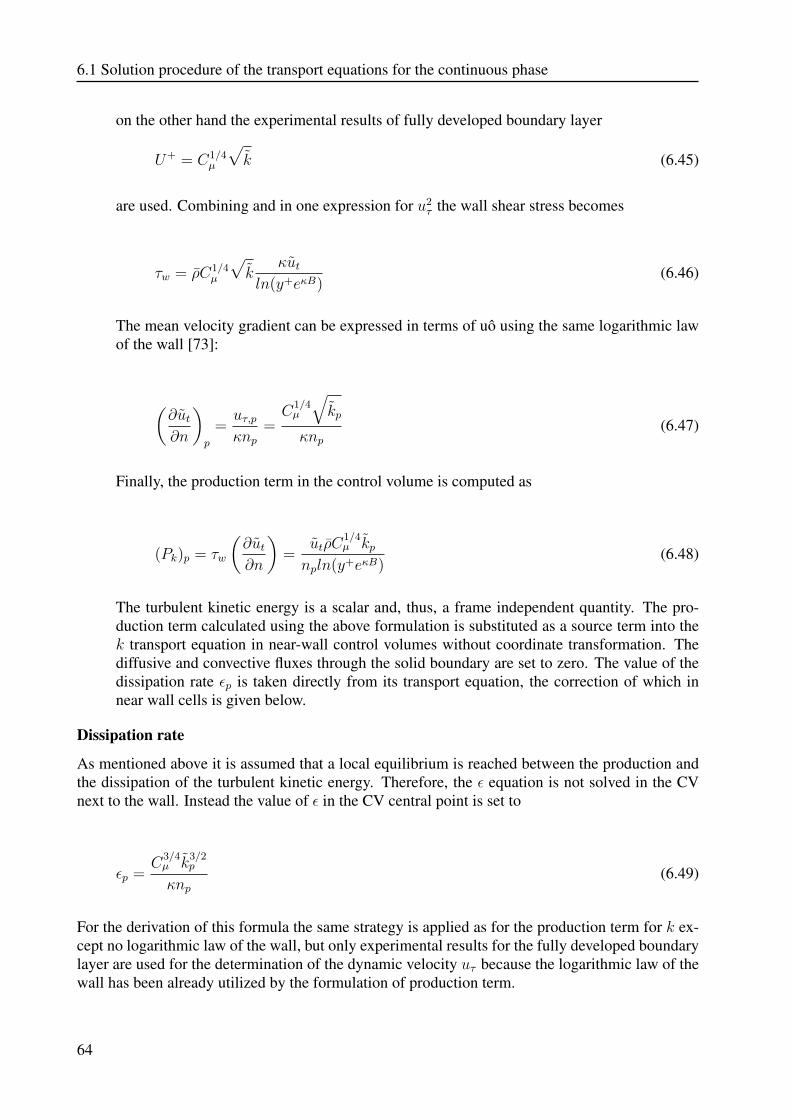
6.1 Solution procedure of the transport equations for the continuous phase
on the other hand the experimental results of fully developed boundary layer
U+ = C1/4µ
√k (6.45)
are used. Combining and in one expression for u2τ the wall shear stress becomes
τw = ρC1/4µ
√k
κutln(y+eκB)
(6.46)
The mean velocity gradient can be expressed in terms of uô using the same logarithmic lawof the wall [73]:
(∂ut∂n
)p
=uτ,pκnp
=C
1/4µ
√kp
κnp(6.47)
Finally, the production term in the control volume is computed as
(Pk)p = τw
(∂ut∂n
)=
utρC1/4µ kp
npln(y+eκB)(6.48)
The turbulent kinetic energy is a scalar and, thus, a frame independent quantity. The pro-duction term calculated using the above formulation is substituted as a source term into thek transport equation in near-wall control volumes without coordinate transformation. Thediffusive and convective fluxes through the solid boundary are set to zero. The value of thedissipation rate εp is taken directly from its transport equation, the correction of which innear wall cells is given below.
Dissipation rate
As mentioned above it is assumed that a local equilibrium is reached between the production andthe dissipation of the turbulent kinetic energy. Therefore, the ε equation is not solved in the CVnext to the wall. Instead the value of ε in the CV central point is set to
εp =C
3/4µ k
3/2p
κnp(6.49)
For the derivation of this formula the same strategy is applied as for the production term for k ex-cept no logarithmic law of the wall, but only experimental results for the fully developed boundarylayer are used for the determination of the dynamic velocity uτ because the logarithmic law of thewall has been already utilized by the formulation of production term.
64
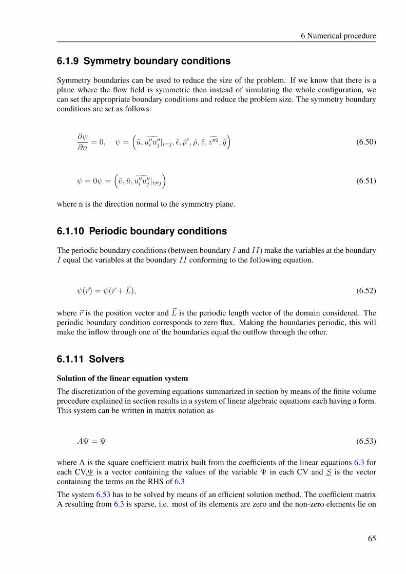
6 Numerical procedure
6.1.9 Symmetry boundary conditions
Symmetry boundaries can be used to reduce the size of the problem. If we know that there is aplane where the flow field is symmetric then instead of simulating the whole configuration, wecan set the appropriate boundary conditions and reduce the problem size. The symmetry boundaryconditions are set as follows:
∂ψ
∂n= 0, ψ =
(u, u′′i u
′′j |i=j, ε, pc, ρ, z, z′′2, y
)(6.50)
ψ = 0ψ =(v, u, u′′i u
′′j |i 6=j
)(6.51)
where n is the direction normal to the symmetry plane.
6.1.10 Periodic boundary conditions
The periodic boundary conditions (between boundary I and II) make the variables at the boundaryI equal the variables at the boundary II conforming to the following equation.
ψ(~r) = ψ(~r + ~L), (6.52)
where ~r is the position vector and ~L is the periodic length vector of the domain considered. Theperiodic boundary condition corresponds to zero flux. Making the boundaries periodic, this willmake the inflow through one of the boundaries equal the outflow through the other.
6.1.11 Solvers
Solution of the linear equation systemThe discretization of the governing equations summarized in section by means of the finite volumeprocedure explained in section results in a system of linear algebraic equations each having a form.This system can be written in matrix notation as
AΨ = Ψ (6.53)
where A is the square coefficient matrix built from the coefficients of the linear equations 6.3 foreach CV,Ψ is a vector containing the values of the variable Ψ in each CV and S is the vectorcontaining the terms on the RHS of 6.3
The system 6.53 has to be solved by means of an efficient solution method. The coefficient matrixA resulting from 6.3 is sparse, i.e. most of its elements are zero and the non-zero elements lie on
65
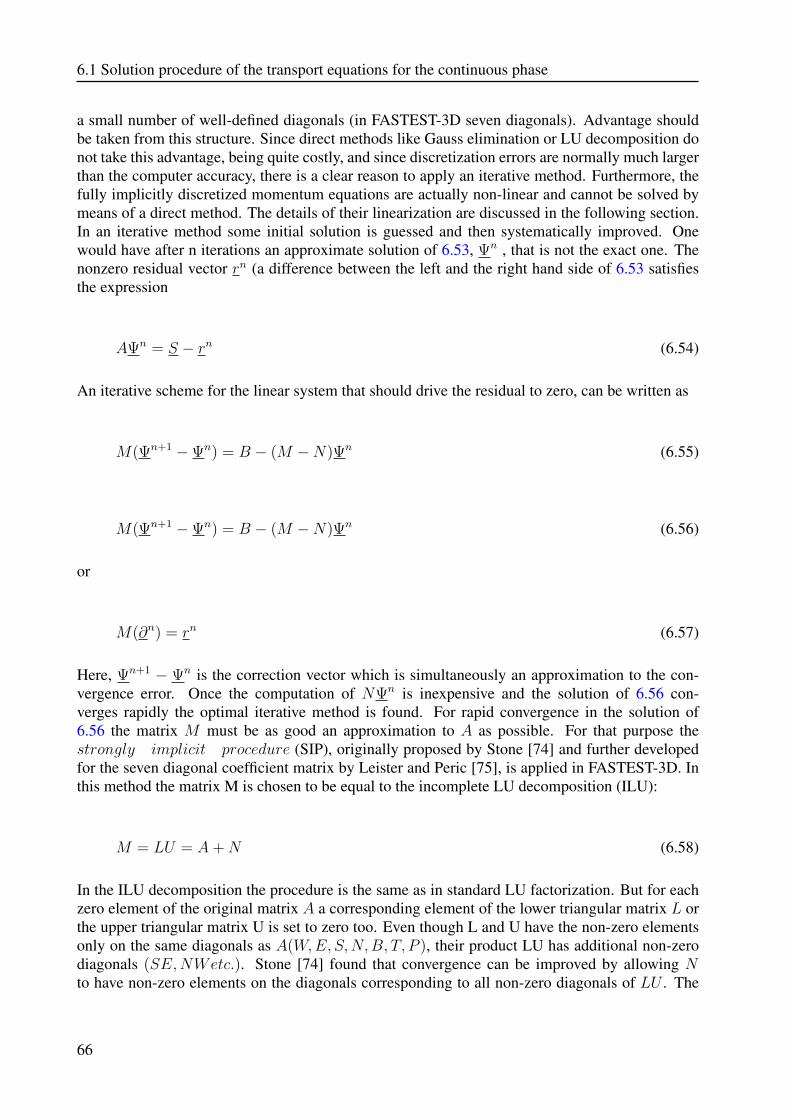
6.1 Solution procedure of the transport equations for the continuous phase
a small number of well-defined diagonals (in FASTEST-3D seven diagonals). Advantage shouldbe taken from this structure. Since direct methods like Gauss elimination or LU decomposition donot take this advantage, being quite costly, and since discretization errors are normally much largerthan the computer accuracy, there is a clear reason to apply an iterative method. Furthermore, thefully implicitly discretized momentum equations are actually non-linear and cannot be solved bymeans of a direct method. The details of their linearization are discussed in the following section.In an iterative method some initial solution is guessed and then systematically improved. Onewould have after n iterations an approximate solution of 6.53, Ψn , that is not the exact one. Thenonzero residual vector rn (a difference between the left and the right hand side of 6.53 satisfiesthe expression
AΨn = S − rn (6.54)
An iterative scheme for the linear system that should drive the residual to zero, can be written as
M(Ψn+1 −Ψn) = B − (M −N)Ψn (6.55)
M(Ψn+1 −Ψn) = B − (M −N)Ψn (6.56)
or
M(∂n) = rn (6.57)
Here, Ψn+1 − Ψn is the correction vector which is simultaneously an approximation to the con-vergence error. Once the computation of NΨn is inexpensive and the solution of 6.56 con-verges rapidly the optimal iterative method is found. For rapid convergence in the solution of6.56 the matrix M must be as good an approximation to A as possible. For that purpose thestrongly implicit procedure (SIP), originally proposed by Stone [74] and further developedfor the seven diagonal coefficient matrix by Leister and Peric [75], is applied in FASTEST-3D. Inthis method the matrix M is chosen to be equal to the incomplete LU decomposition (ILU):
M = LU = A+N (6.58)
In the ILU decomposition the procedure is the same as in standard LU factorization. But for eachzero element of the original matrix A a corresponding element of the lower triangular matrix L orthe upper triangular matrix U is set to zero too. Even though L and U have the non-zero elementsonly on the same diagonals as A(W,E, S,N,B, T, P ), their product LU has additional non-zerodiagonals (SE,NWetc.). Stone [74] found that convergence can be improved by allowing Nto have non-zero elements on the diagonals corresponding to all non-zero diagonals of LU . The
66
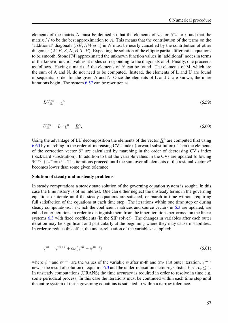
6 Numerical procedure
elements of the matrix N must be defined so that the elements of vector NΨ ≈ 0 and that thematrix M to be the best approximation to A. This means that the contribution of the terms on the’additional’ diagonals (SE,NWetc.) in N must be nearly cancelled by the contribution of otherdiagonals (W,E, S,N,B, T, P ). Expecting the solution of the elliptic partial differential equationsto be smooth, Stone [74] approximated the unknown function values in ’additional’ nodes in termsof the known function values at nodes corresponding to the diagonals of A. Finally, one proceedsas follows. Having a matrix A the elements of N can be found. The elements of M, which arethe sum of A and N, do not need to be computed. Instead, the elements of L and U are foundin sequential order for the given A and N. Once the elements of L and U are known, the inneriterations begin. The system 6.57 can be rewritten as
LU∂n = rn (6.59)
U∂n = L−1rn = Rn. (6.60)
Using the advantage of LU decomposition the elements of the vector Rn are computed first using6.60 by marching in the order of increasing CV’s index (forward substitution). Then the elementsof the correction vector ∂n are calculated by marching in the order of decreasing CV’s index(backward substitution). In addition to that the variable values in the CVs are updated followingΨn+1 + Ψn = ∂n . The iterations proceed until the sum over all elements of the residual vector rn
becomes lower than some given tolerance.
Solution of steady and unsteady problems
In steady computations a steady state solution of the governing equation system is sought. In thiscase the time history is of no interest. One can either neglect the unsteady terms in the governingequations or iterate until the steady equations are satisfied, or march in time without requiringfull satisfaction of the equations at each time step. The iterations within one time step or duringsteady computations, in which the coefficient matrices and source vectors in 6.3 are updated, arecalled outer iterations in order to distinguish them from the inner iterations performed on the linearsystems 6.3 with fixed coefficients (in the SIP solver). The changes in variables after each outeriteration may be significant and particularly at the beginning where they may cause instabilities.In order to reduce this effect the under-relaxation of the variables is applied:
ψm = ψm+1 + αψ(ψm − ψm−1) (6.61)
where ψm and ψm−1 are the values of the variable ψ after m-th and (m- 1)st outer iteration, ψnew
new is the result of solution of equation 6.3 and the under-relaxation factor αψ satisfies 0 < αψ ≤ 1.In unsteady computations (URANS) the time accuracy is required in order to resolve in time e.g.some periodical process. In this case the iterations must be continued within each time step untilthe entire system of these governing equations is satisfied to within a narrow tolerance.
67
6.2 Numerical method of the transport equations for the dispersed phase
6.2 Numerical method of the transport equations for thedispersed phase
6.2.1 Solving the equation of motion and time discretization
Since equation 4.3 is an ordinary differential equation, it can be solved by using classical numericalmethods such as Euler’s forward integration method [72]:
xn+1i = xni + ∂tuni , (6.62)
un+1di
= undi +∂t
md
∑F ni , (6.63)
where xi and udi denote the parcel location and velocity component respectively. From one giventime point ( tn ), it is possible to find the next point at a given time step ( tn+1 ) along the samestreamline and thus tracking the whole line. The Euler’s forward method is fast but strongly de-pends on the quality of the initial velocity field. In some situations, it may lead to spirals. Then,additional stopping conditions must be added to avoid such situations. Moreover, in zones wherethe velocity orientation changes, the streamline presents a high curvature and its trajectory is notnecessarily parallel to the initial velocity field. The Euler’s method is a simple approach to imple-ment. However, it has a low accuracy, as it is a first order method. If one wishes to compute veryaccurate solutions or solutions that are accurate over a long interval, then Euler’s method (used forthe dispersed phase in this work≈ equation 4.3- ) requires a large number of small steps. (accuracy≈ dt), but thus one rends the simulation time impractically long.
Other time integration methods often used in literature are Runge Kutta method [126] and thebackward Euler method [72], which are implicit. These methods require the resolution of a linearsystem per iteration, as well as the storage of the system state added to those required for thesystem resolution algorithm. These methods are supposed to provide approximate results thatare not subject to numerical instability as the time step is increased [72]. As mentioned above,time steps within Euler’s forward method, are limited by the conditions for physical processes andnumerical stability according to:
∂t = 0.1 min(τp, TE, TW , TCV ), (6.64)
where τp denotes the particle relaxation time, defined in section 4.2, and TE is the turbulent integraltime scale
TE = cTk
ε(6.65)
68
6 Numerical procedure
The variable TW is the time required by a parcel to traverse a turbulent eddy
TW =LE
|~u− ~ud|,
(LE = TE
√2
3k
), (6.66)
and the variable TCV represents the time taken by a parcel to cross the entire control volume.
TCV =∂xi|udi |
(6.67)
6.2.2 Statistical sampling
Similarly to the Eulerian part where equations averaged for flow quantities (velocity, mass fraction,temperature, etc) are solved, in the Lagrangian part momentanous quantities are to be sampled andaveraged. Mean values and variances of droplet characteristic variables (velocity components,diameter, temperature, etc.) are evaluated in each cell according to [39]:
φd =
∑Kdk=1
(∑NCVn=1 φd,i,j,kNd,k
)∑Kd
k=1NCV
(6.68)
(φ′d)2 =
∑Kdk=1
(∑NCVn=1 φ
2d,i,j,kNd,k
)∑Kd
k=1NCV
− (φd) (6.69)
whereKd is the total number of numerical droplets in a considered cell,NCV represents the numberof time steps which a droplet needs while crossing the cell and Nd,k is the number of real particlesrepresented by a numerical one. One should mention here that the total number of particles/dropletswithin a control volume represents an important factor for the accuracy of statistics of dispersedphase properties. In order to secure smooth distribution of results, the variables Nd,k is desirednot to exceed 103, as pointed out in [39]. Nevertheless, regions where particles/droplets are notable to reach, due to high shear flow or due to total evaporation, are characterized by non-uniformproperty profiles. The particles/droplets mass concentration within a control volume is computedin the following way:
σd =
Kd∑k=1
(NCV∑n=1
mdNd,k
~ud,k∂Aj∂tin
)(6.70)
where ∂Aj denoted the cross section area of the considered control volume, ∂tin represents areference time, which specifies the droplets/particles mass flow at the boundary conditions.
69
6.3 Euler-Lagrange coupling and underrelaxation of dispersed phase source terms
Though the results from URANS are unsteady, one is often interested only in the time-averagedflow. Coherent motion of the velocity component can then be decomposed in
U =⟨U⟩
(x) + u′(x, t) + u′′(x, t) (6.71)
⟨U⟩
is the time averaged velocity, u′ is the deviation of the phase averaged from the time averagedvelocity component and u′′ is the turbulent fluctuation.
The time averaged mean velocity component is obtained by averaging all time steps N as
⟨U⟩
=1
N
k=1∑N
⟨U⟩
(x) + u′(x, t). (6.72)
6.3 Euler-Lagrange coupling and underrelaxation ofdispersed phase source terms
6.3.1 Steady coupling
Numerically, the interaction between the continuous and the dispersed phases is taken into accountby means of several couplings between the two modules involved. Following a steady method,after several iterations of gas phase alone, the gas variables are kept frozen and all the particlesrepresenting the particles are injected in the computational domain. The computed particle sourceterms are inserted in the calculations of gas phase and kept frozen till the next coupling takes placein which the old particle sources are replaced by newly calculated sources. The particle sourceterms has to be inserted in the calculation of the gas phase to ensure the full two-way physicalcoupling as permitted by a mean concentration of particles shown in figures 6.5. High levels ofunder-relaxation technique were used in order to obtain successful convergence (Chrigui et al.2004, Sadiki et al. 2005, Kohnen et al. 1994). Due to the presence of particles source terms, theconventional residuals are characterized by a jump of residuals after each coupling. To avoid it, anadditional under-relaxation technique should also be employed for particle source terms (Kohnenet al. 1994).
Si+1φp = Siφp ∗ (1− γ) + Si+1
φp(cal.) ∗ γ (6.73)
where Si+1φp and Siφp are the particle source terms appearing at i+1th and ith couplings, respec-
tively. The under-relaxation factor γ takes values in the interval [0,1]. In the frame of this work,convergence of the Eulerian-Lagrangian coupling procedure is reached when the fluid’s propertiesdo not change their value from one coupling to the next in the presence of particles. This wasmainly achieved after 10 couplings. Figure 6.5 shows the procedure of the steady coupling. Firstthe carrier flow equations are solved in steady mode to reach the converged solution for statisticalquantities without presence of particles. The particle motion equation would then be called and
70
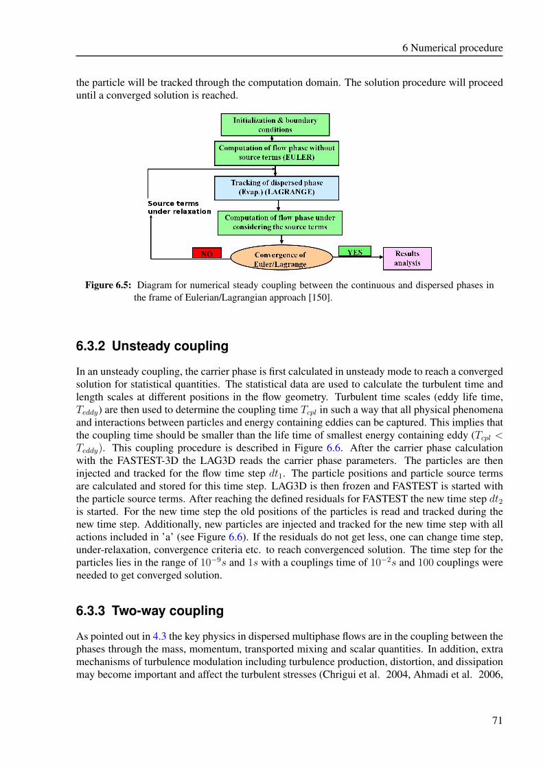
6 Numerical procedure
the particle will be tracked through the computation domain. The solution procedure will proceeduntil a converged solution is reached.
Figure 6.5: Diagram for numerical steady coupling between the continuous and dispersed phases inthe frame of Eulerian/Lagrangian approach [150].
6.3.2 Unsteady coupling
In an unsteady coupling, the carrier phase is first calculated in unsteady mode to reach a convergedsolution for statistical quantities. The statistical data are used to calculate the turbulent time andlength scales at different positions in the flow geometry. Turbulent time scales (eddy life time,Teddy) are then used to determine the coupling time Tcpl in such a way that all physical phenomenaand interactions between particles and energy containing eddies can be captured. This implies thatthe coupling time should be smaller than the life time of smallest energy containing eddy (Tcpl <Teddy). This coupling procedure is described in Figure 6.6. After the carrier phase calculationwith the FASTEST-3D the LAG3D reads the carrier phase parameters. The particles are theninjected and tracked for the flow time step dt1. The particle positions and particle source termsare calculated and stored for this time step. LAG3D is then frozen and FASTEST is started withthe particle source terms. After reaching the defined residuals for FASTEST the new time step dt2is started. For the new time step the old positions of the particles is read and tracked during thenew time step. Additionally, new particles are injected and tracked for the new time step with allactions included in ’a’ (see Figure 6.6). If the residuals do not get less, one can change time step,under-relaxation, convergence criteria etc. to reach convergenced solution. The time step for theparticles lies in the range of 10−9s and 1s with a couplings time of 10−2s and 100 couplings wereneeded to get converged solution.
6.3.3 Two-way coupling
As pointed out in 4.3 the key physics in dispersed multiphase flows are in the coupling between thephases through the mass, momentum, transported mixing and scalar quantities. In addition, extramechanisms of turbulence modulation including turbulence production, distortion, and dissipationmay become important and affect the turbulent stresses (Chrigui et al. 2004, Ahmadi et al. 2006,
71
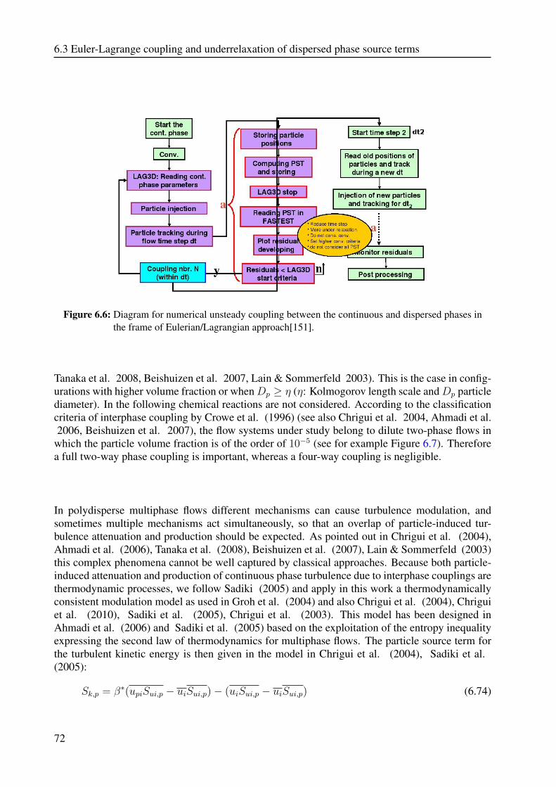
6.3 Euler-Lagrange coupling and underrelaxation of dispersed phase source terms
Figure 6.6: Diagram for numerical unsteady coupling between the continuous and dispersed phases inthe frame of Eulerian/Lagrangian approach[151].
Tanaka et al. 2008, Beishuizen et al. 2007, Lain & Sommerfeld 2003). This is the case in config-urations with higher volume fraction or whenDp ≥ η (η: Kolmogorov length scale andDp particlediameter). In the following chemical reactions are not considered. According to the classificationcriteria of interphase coupling by Crowe et al. (1996) (see also Chrigui et al. 2004, Ahmadi et al.2006, Beishuizen et al. 2007), the flow systems under study belong to dilute two-phase flows in
which the particle volume fraction is of the order of 10−5 (see for example Figure 6.7). Thereforea full two-way phase coupling is important, whereas a four-way coupling is negligible.
In polydisperse multiphase flows different mechanisms can cause turbulence modulation, andsometimes multiple mechanisms act simultaneously, so that an overlap of particle-induced tur-bulence attenuation and production should be expected. As pointed out in Chrigui et al. (2004),Ahmadi et al. (2006), Tanaka et al. (2008), Beishuizen et al. (2007), Lain & Sommerfeld (2003)this complex phenomena cannot be well captured by classical approaches. Because both particle-induced attenuation and production of continuous phase turbulence due to interphase couplings arethermodynamic processes, we follow Sadiki (2005) and apply in this work a thermodynamicallyconsistent modulation model as used in Groh et al. (2004) and also Chrigui et al. (2004), Chriguiet al. (2010), Sadiki et al. (2005), Chrigui et al. (2003). This model has been designed inAhmadi et al. (2006) and Sadiki et al. (2005) based on the exploitation of the entropy inequalityexpressing the second law of thermodynamics for multiphase flows. The particle source term forthe turbulent kinetic energy is then given in the model in Chrigui et al. (2004), Sadiki et al.(2005):
Sk,p = β∗(upiSui,p − uiSui,p)− (uiSui,p − uiSui,p) (6.74)
72
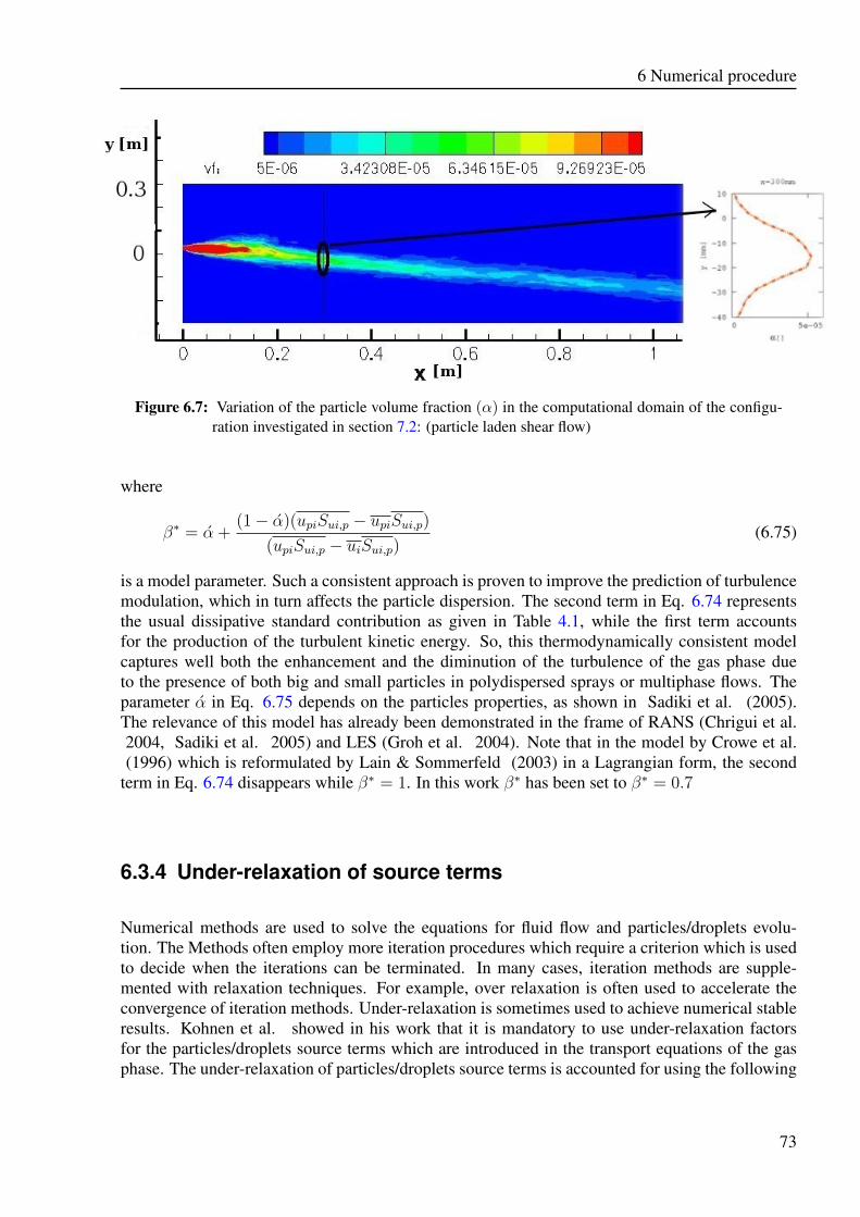
6 Numerical procedure
Figure 6.7: Variation of the particle volume fraction (α) in the computational domain of the configu-ration investigated in section 7.2: (particle laden shear flow)
where
β∗ = α +(1− α)(upiSui,p − upiSui,p)
(upiSui,p − uiSui,p)(6.75)
is a model parameter. Such a consistent approach is proven to improve the prediction of turbulencemodulation, which in turn affects the particle dispersion. The second term in Eq. 6.74 representsthe usual dissipative standard contribution as given in Table 4.1, while the first term accountsfor the production of the turbulent kinetic energy. So, this thermodynamically consistent modelcaptures well both the enhancement and the diminution of the turbulence of the gas phase dueto the presence of both big and small particles in polydispersed sprays or multiphase flows. Theparameter α in Eq. 6.75 depends on the particles properties, as shown in Sadiki et al. (2005).The relevance of this model has already been demonstrated in the frame of RANS (Chrigui et al.2004, Sadiki et al. 2005) and LES (Groh et al. 2004). Note that in the model by Crowe et al.(1996) which is reformulated by Lain & Sommerfeld (2003) in a Lagrangian form, the second
term in Eq. 6.74 disappears while β∗ = 1. In this work β∗ has been set to β∗ = 0.7
6.3.4 Under-relaxation of source terms
Numerical methods are used to solve the equations for fluid flow and particles/droplets evolu-tion. The Methods often employ more iteration procedures which require a criterion which is usedto decide when the iterations can be terminated. In many cases, iteration methods are supple-mented with relaxation techniques. For example, over relaxation is often used to accelerate theconvergence of iteration methods. Under-relaxation is sometimes used to achieve numerical stableresults. Kohnen et al. showed in his work that it is mandatory to use under-relaxation factorsfor the particles/droplets source terms which are introduced in the transport equations of the gasphase. The under-relaxation of particles/droplets source terms is accounted for using the following
73
6.3 Euler-Lagrange coupling and underrelaxation of dispersed phase source terms
expression:
Si+1φ,p(considered) = αSi+1
φ,p + (1− α)Siφ,p. (6.76)
Here Si+1φ,p is the new computed particles/droplets source terms within the iteration (i+1), whereas
Siφ,p is the old source terms (previous iteration) and Si+1φ,p(considered) the source terms account for the
carrier phase. The variable α indicates the under-relaxation factor, which vary between zero andone. It is defined by user and cannot influence the numerical results once convergence reached.
The goal of introducing under-relaxation factors is to enhance the numerical stability and to accel-erate the convergence of the Eulerian- Lagrangian coupling. Sommerfeld [25] mentioned that anunderrelaxation factor of 0.1 was required for his work to get a stable numerical computation andthat the total Eulerian-Lagrangian coupling was between 30 and 50 iterations.
74
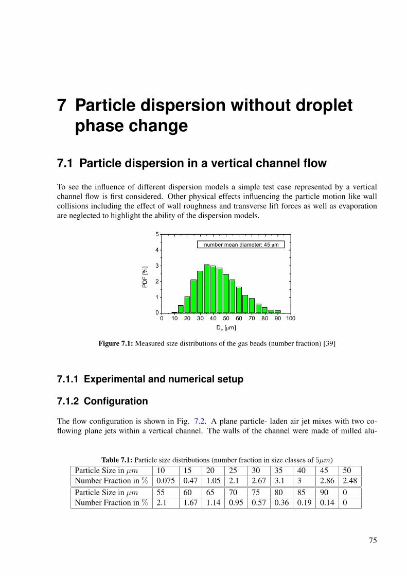
7 Particle dispersion without dropletphase change
7.1 Particle dispersion in a vertical channel flow
To see the influence of different dispersion models a simple test case represented by a verticalchannel flow is first considered. Other physical effects influencing the particle motion like wallcollisions including the effect of wall roughness and transverse lift forces as well as evaporationare neglected to highlight the ability of the dispersion models.
Figure 7.1: Measured size distributions of the gas beads (number fraction) [39]
7.1.1 Experimental and numerical setup
7.1.2 Configuration
The flow configuration is shown in Fig. 7.2. A plane particle- laden air jet mixes with two co-flowing plane jets within a vertical channel. The walls of the channel were made of milled alu-
Table 7.1: Particle size distributions (number fraction in size classes of 5µm)Particle Size in µm 10 15 20 25 30 35 40 45 50Number Fraction in % 0.075 0.47 1.05 2.1 2.67 3.1 3 2.86 2.48Particle Size in µm 55 60 65 70 75 80 85 90 0Number Fraction in % 2.1 1.67 1.14 0.95 0.57 0.36 0.19 0.14 0
75
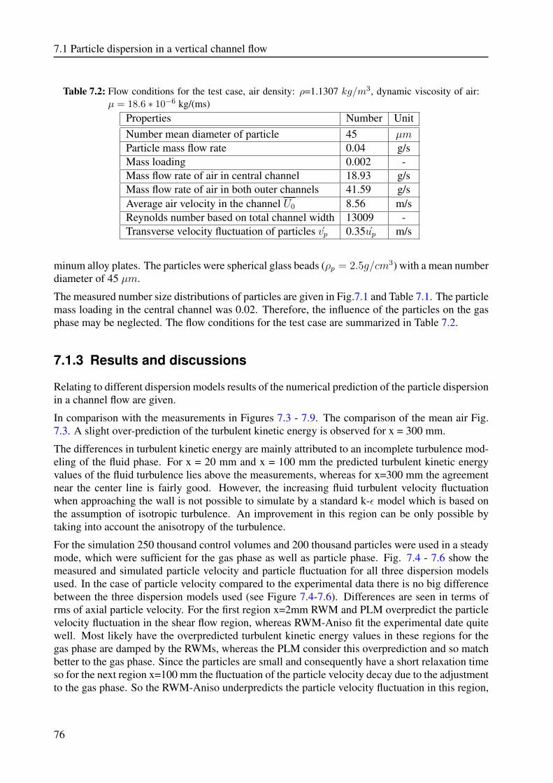
7.1 Particle dispersion in a vertical channel flow
Table 7.2: Flow conditions for the test case, air density: ρ=1.1307 kg/m3, dynamic viscosity of air:µ = 18.6 ∗ 10−6 kg/(ms)
Properties Number UnitNumber mean diameter of particle 45 µmParticle mass flow rate 0.04 g/sMass loading 0.002 -Mass flow rate of air in central channel 18.93 g/sMass flow rate of air in both outer channels 41.59 g/sAverage air velocity in the channel U0 8.56 m/sReynolds number based on total channel width 13009 -Transverse velocity fluctuation of particles vp 0.35up m/s
minum alloy plates. The particles were spherical glass beads (ρp = 2.5g/cm3) with a mean numberdiameter of 45 µm.
The measured number size distributions of particles are given in Fig.7.1 and Table 7.1. The particlemass loading in the central channel was 0.02. Therefore, the influence of the particles on the gasphase may be neglected. The flow conditions for the test case are summarized in Table 7.2.
7.1.3 Results and discussions
Relating to different dispersion models results of the numerical prediction of the particle dispersionin a channel flow are given.
In comparison with the measurements in Figures 7.3 - 7.9. The comparison of the mean air Fig.7.3. A slight over-prediction of the turbulent kinetic energy is observed for x = 300 mm.
The differences in turbulent kinetic energy are mainly attributed to an incomplete turbulence mod-eling of the fluid phase. For x = 20 mm and x = 100 mm the predicted turbulent kinetic energyvalues of the fluid turbulence lies above the measurements, whereas for x=300 mm the agreementnear the center line is fairly good. However, the increasing fluid turbulent velocity fluctuationwhen approaching the wall is not possible to simulate by a standard k-ε model which is based onthe assumption of isotropic turbulence. An improvement in this region can be only possible bytaking into account the anisotropy of the turbulence.
For the simulation 250 thousand control volumes and 200 thousand particles were used in a steadymode, which were sufficient for the gas phase as well as particle phase. Fig. 7.4 - 7.6 show themeasured and simulated particle velocity and particle fluctuation for all three dispersion modelsused. In the case of particle velocity compared to the experimental data there is no big differencebetween the three dispersion models used (see Figure 7.4-7.6). Differences are seen in terms ofrms of axial particle velocity. For the first region x=2mm RWM and PLM overpredict the particlevelocity fluctuation in the shear flow region, whereas RWM-Aniso fit the experimental date quitewell. Most likely have the overpredicted turbulent kinetic energy values in these regions for thegas phase are damped by the RWMs, whereas the PLM consider this overprediction and so matchbetter to the gas phase. Since the particles are small and consequently have a short relaxation timeso for the next region x=100 mm the fluctuation of the particle velocity decay due to the adjustmentto the gas phase. So the RWM-Aniso underpredicts the particle velocity fluctuation in this region,
76
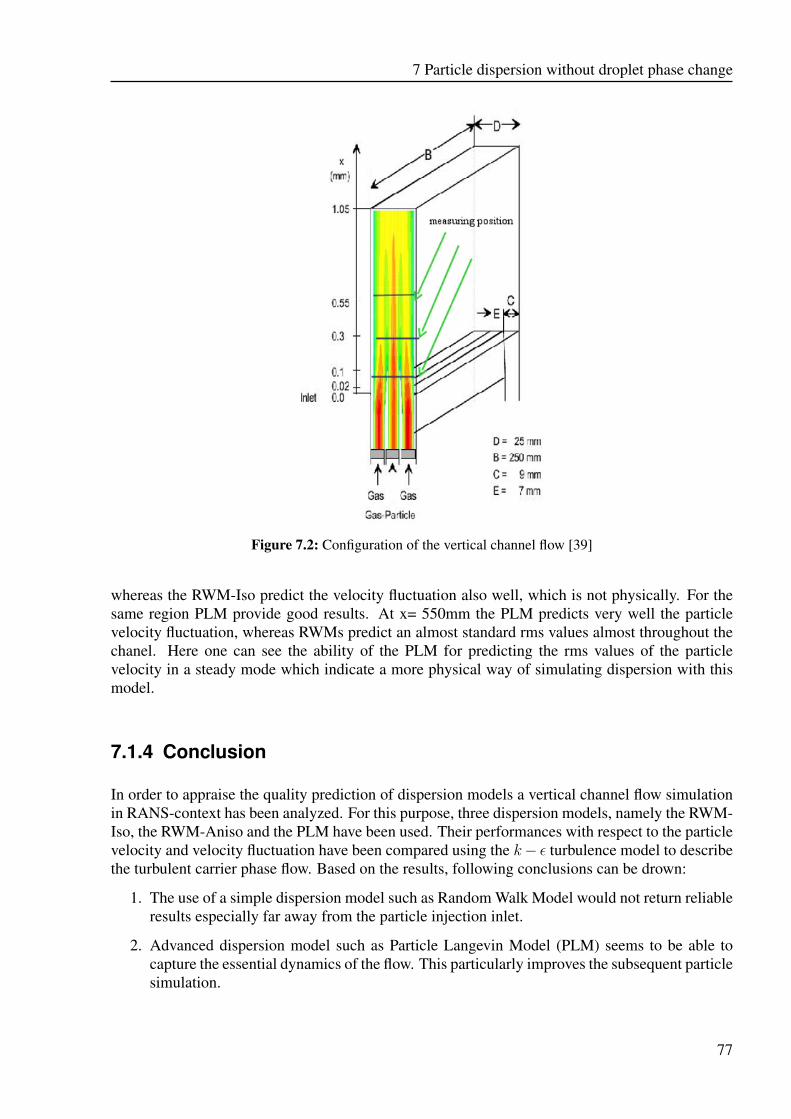
7 Particle dispersion without droplet phase change
Figure 7.2: Configuration of the vertical channel flow [39]
whereas the RWM-Iso predict the velocity fluctuation also well, which is not physically. For thesame region PLM provide good results. At x= 550mm the PLM predicts very well the particlevelocity fluctuation, whereas RWMs predict an almost standard rms values almost throughout thechanel. Here one can see the ability of the PLM for predicting the rms values of the particlevelocity in a steady mode which indicate a more physical way of simulating dispersion with thismodel.
7.1.4 Conclusion
In order to appraise the quality prediction of dispersion models a vertical channel flow simulationin RANS-context has been analyzed. For this purpose, three dispersion models, namely the RWM-Iso, the RWM-Aniso and the PLM have been used. Their performances with respect to the particlevelocity and velocity fluctuation have been compared using the k− ε turbulence model to describethe turbulent carrier phase flow. Based on the results, following conclusions can be drown:
1. The use of a simple dispersion model such as Random Walk Model would not return reliableresults especially far away from the particle injection inlet.
2. Advanced dispersion model such as Particle Langevin Model (PLM) seems to be able tocapture the essential dynamics of the flow. This particularly improves the subsequent particlesimulation.
77
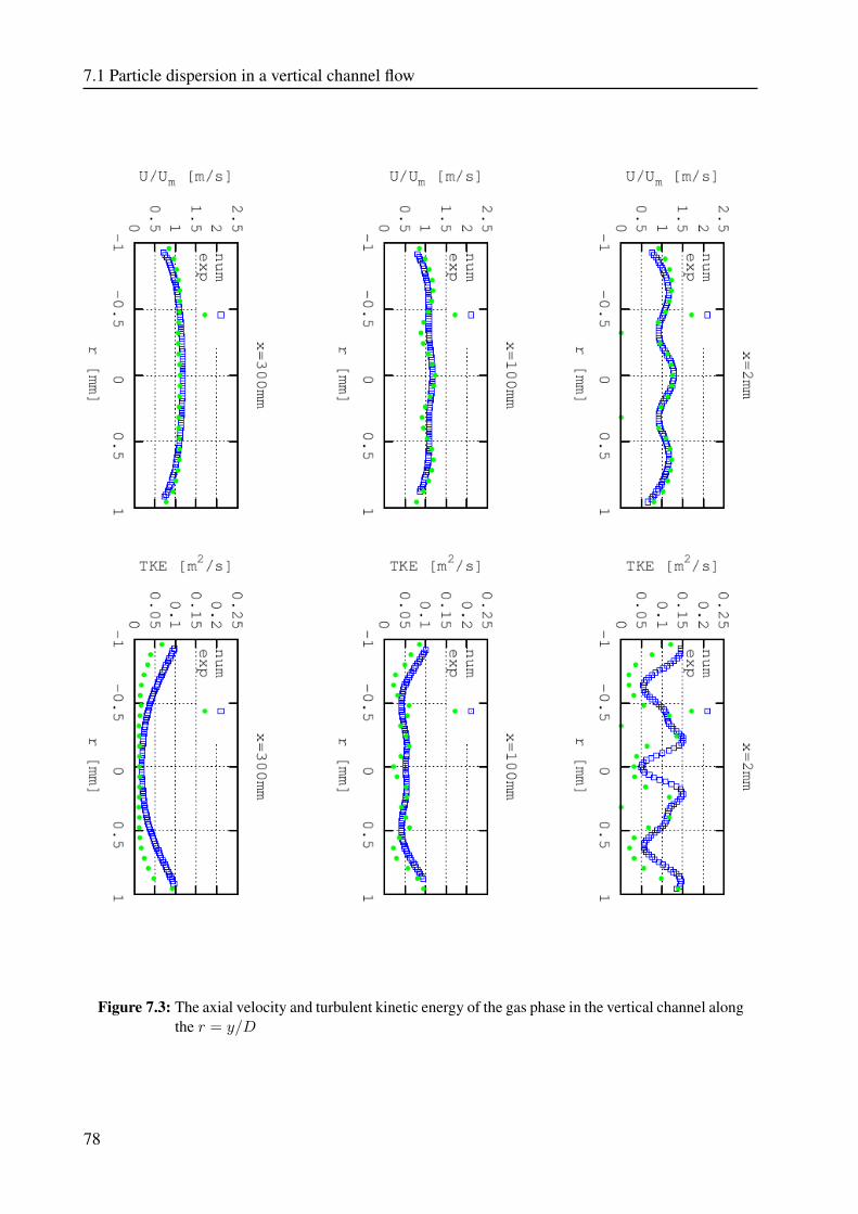
7.1 Particle dispersion in a vertical channel flow
Figure 7.3: The axial velocity and turbulent kinetic energy of the gas phase in the vertical channel alongthe r = y/D
78
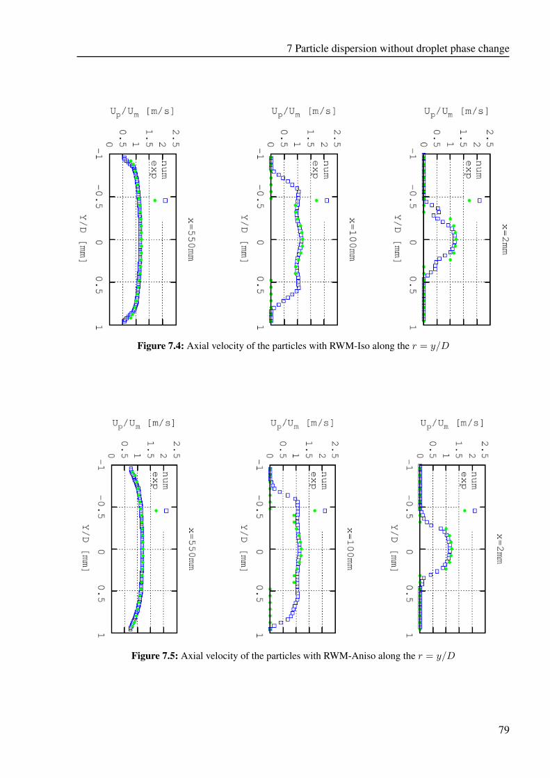
7 Particle dispersion without droplet phase change
Figure 7.4: Axial velocity of the particles with RWM-Iso along the r = y/D
Figure 7.5: Axial velocity of the particles with RWM-Aniso along the r = y/D
79
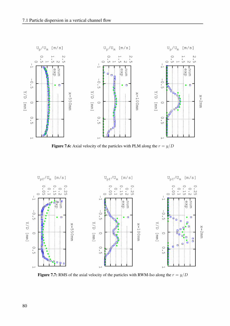
7.1 Particle dispersion in a vertical channel flow
Figure 7.6: Axial velocity of the particles with PLM along the r = y/D
Figure 7.7: RMS of the axial velocity of the particles with RWM-Iso along the r = y/D
80
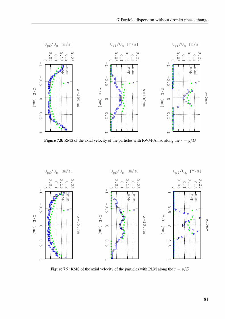
7 Particle dispersion without droplet phase change
Figure 7.8: RMS of the axial velocity of the particles with RWM-Aniso along the r = y/D
Figure 7.9: RMS of the axial velocity of the particles with PLM along the r = y/D
81
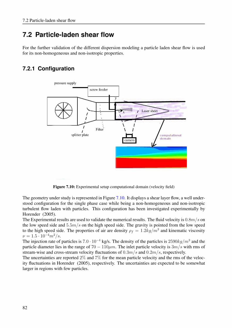
7.2 Particle-laden shear flow
7.2 Particle-laden shear flow
For the further validation of the different dispersion modeling a particle laden shear flow is usedfor its non-homogeneous and non-isotropic properties.
7.2.1 Configuration
Figure 7.10: Experimental setup computational domain (velocity field)
The geometry under study is represented in Figure 7.10. It displays a shear layer flow, a well under-stood configuration for the single phase case while being a non-homogeneous and non-isotropicturbulent flow laden with particles. This configuration has been investigated experimentally byHorender (2005).The Experimental results are used to validate the numerical results. The fluid velocity is 0.8m/s onthe low speed side and 5.5m/s on the high speed side. The gravity is pointed from the low speedto the high speed side. The properties of air are density ρf = 1.2kg/m3 and kinematic viscosityν = 1.5 · 10−4m2/s.The injection rate of particles is 7.0 · 10−4 kg/s. The density of the particles is 2590kg/m3 and theparticle diameter lies in the range of 70− 110µm. The inlet particle velocity is 3m/s with rms ofstream-wise and cross-stream velocity fluctuations of 0.3m/s and 0.2m/s, respectively.The uncertainties are reported 2% and 7% for the mean particle velocity and the rms of the veloc-ity fluctuations in Horender (2005), respectively. The uncertainties are expected to be somewhatlarger in regions with few particles.
82
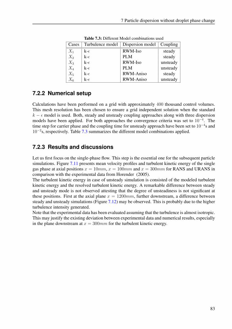
7 Particle dispersion without droplet phase change
Table 7.3: Different Model combinations usedCases Turbulence model Dispersion model CouplingX1 k-ε RWM-Iso steadyX2 k-ε PLM steadyX3 k-ε RWM-Iso unsteadyX4 k-ε PLM unsteadyX5 k-ε RWM-Aniso steadyX6 k-ε RWM-Aniso unsteady
7.2.2 Numerical setup
Calculations have been performed on a grid with approximately 400 thousand control volumes.This mesh resolution has been chosen to ensure a grid independent solution when the standardk − ε model is used. Both, steady and unsteady coupling approaches along with three dispersionmodels have been applied. For both approaches the convergence criteria was set to 10−4. Thetime step for carrier phase and the coupling time for unsteady approach have been set to 10−4s and10−2s, respectively. Table 7.3 summarizes the different model combinations applied.
7.2.3 Results and discussions
Let us first focus on the single-phase flow. This step is the essential one for the subsequent particlesimulations. Figure 7.11 presents mean velocity profiles and turbulent kinetic energy of the singlegas phase at axial positions x = 10mm, x = 100mm and x = 300mm for RANS and URANS incomparison with the experimental data from Horender (2005).The turbulent kinetic energy in case of unsteady simulation is consisted of the modeled turbulentkinetic energy and the resolved turbulent kinetic energy. A remarkable difference between steadyand unsteady mode is not observed attesting that the degree of unsteadiness is not significant atthese positions. First at the axial plane x = 1200mm, further downstream, a difference betweensteady and unsteady simulations (Figure 7.12) may be observed. This is probably due to the higherturbulence intensity generated.Note that the experimental data has been evaluated assuming that the turbulence is almost isotropic.This may justify the existing deviation between experimental data and numerical results, especiallyin the plane downstream at x = 300mm for the turbulent kinetic energy.
83
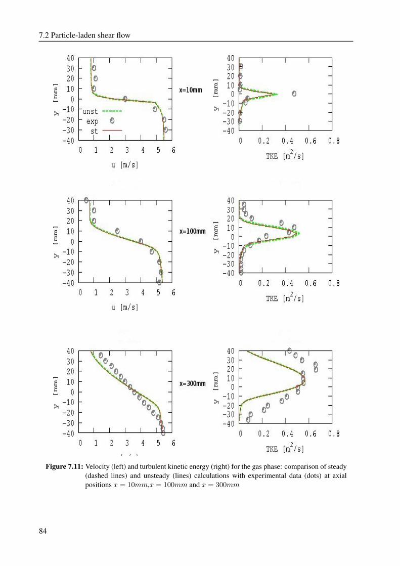
7.2 Particle-laden shear flow
Figure 7.11: Velocity (left) and turbulent kinetic energy (right) for the gas phase: comparison of steady(dashed lines) and unsteady (lines) calculations with experimental data (dots) at axialpositions x = 10mm,x = 100mm and x = 300mm
84
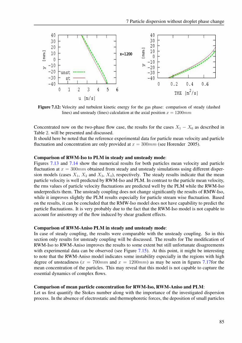
7 Particle dispersion without droplet phase change
Figure 7.12: Velocity and turbulent kinetic energy for the gas phase: comparison of steady (dashedlines) and unsteady (lines) calculation at the axial position x = 1200mm
Concentrated now on the two-phase flow case, the results for the cases X1 − X6 as described inTable 2. will be presented and discussed.It should here be noted that the reference experimental data for particle mean velocity and particlefluctuation and concentration are only provided at x = 300mm (see Horender 2005).
Comparison of RWM-Iso to PLM in steady and unsteady mode:Figures 7.13 and 7.14 show the numerical results for both particles mean velocity and particlefluctuation at x = 300mm obtained from steady and unsteady simulations using different disper-sion models (cases X1, X2 and X3, X4), respectively. The steady results indicate that the meanparticle velocity is well predicted by RWM-Iso and PLM. In contrast to the particle mean velocity,the rms values of particle velocity fluctuations are predicted well by the PLM while the RWM-Isounderpredicts them. The unsteady coupling does not change significantly the results of RMW-Iso,while it improves slightly the PLM results especially for particle stream wise fluctuation. Basedon the results, it can be concluded that the RMW-Iso model does not have capability to predict theparticle fluctuations. It is very probably due to the fact that the RWM-Iso model is not capable toaccount for anisotropy of the flow induced by shear gradient effects.
Comparison of RWM-Aniso PLM in steady and unsteady mode:In case of steady coupling, the results were comparable with the unsteady coupling. So in thissection only results for unsteady coupling will be discussed. The results for The modification ofRWM-Iso to RWM-Aniso improves the results to some extent but still unfortunate disagreementswith experimental data can be observed (see Figure 7.15). At this point, it might be interestingto note that the RWM-Aniso model indicates some instability especially in the regions with highdegree of unsteadiness (x = 700mm and x = 1200mm) as may be seen in figures 7.17for themean concentration of the particles. This may reveal that this model is not capable to capture theessential dynamics of complex flows.
Comparison of mean particle concentration for RWM-Iso, RWM-Aniso and PLM:Let us first quantify the Stokes number along with the importance of the investigated dispersionprocess. In the absence of electrostatic and thermophoretic forces, the deposition of small particles
85
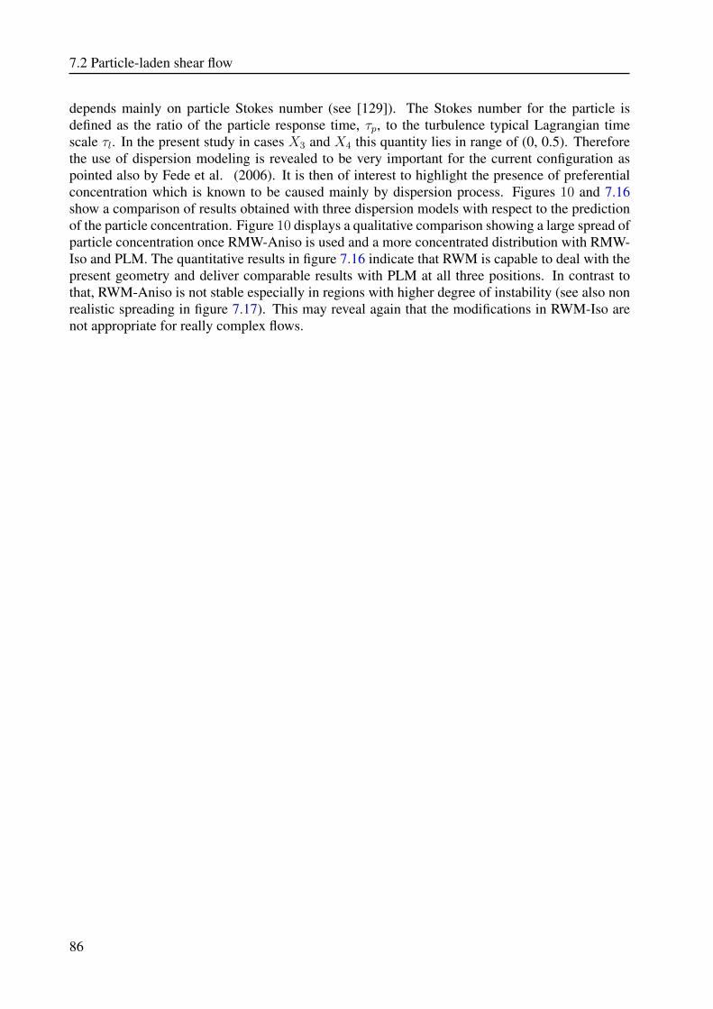
7.2 Particle-laden shear flow
depends mainly on particle Stokes number (see [129]). The Stokes number for the particle isdefined as the ratio of the particle response time, τp, to the turbulence typical Lagrangian timescale τl. In the present study in cases X3 and X4 this quantity lies in range of (0, 0.5). Thereforethe use of dispersion modeling is revealed to be very important for the current configuration aspointed also by Fede et al. (2006). It is then of interest to highlight the presence of preferentialconcentration which is known to be caused mainly by dispersion process. Figures 10 and 7.16show a comparison of results obtained with three dispersion models with respect to the predictionof the particle concentration. Figure 10 displays a qualitative comparison showing a large spread ofparticle concentration once RMW-Aniso is used and a more concentrated distribution with RMW-Iso and PLM. The quantitative results in figure 7.16 indicate that RWM is capable to deal with thepresent geometry and deliver comparable results with PLM at all three positions. In contrast tothat, RWM-Aniso is not stable especially in regions with higher degree of instability (see also nonrealistic spreading in figure 7.17). This may reveal again that the modifications in RWM-Iso arenot appropriate for really complex flows.
86
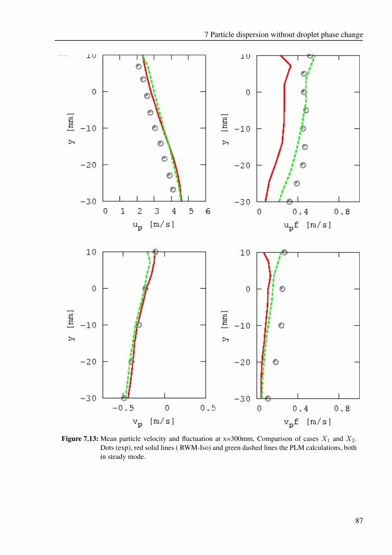
7 Particle dispersion without droplet phase change
Figure 7.13: Mean particle velocity and fluctuation at x=300mm, Comparison of cases X1 and X2.Dots (exp), red solid lines ( RWM-Iso) and green dashed lines the PLM calculations, bothin steady mode.
87
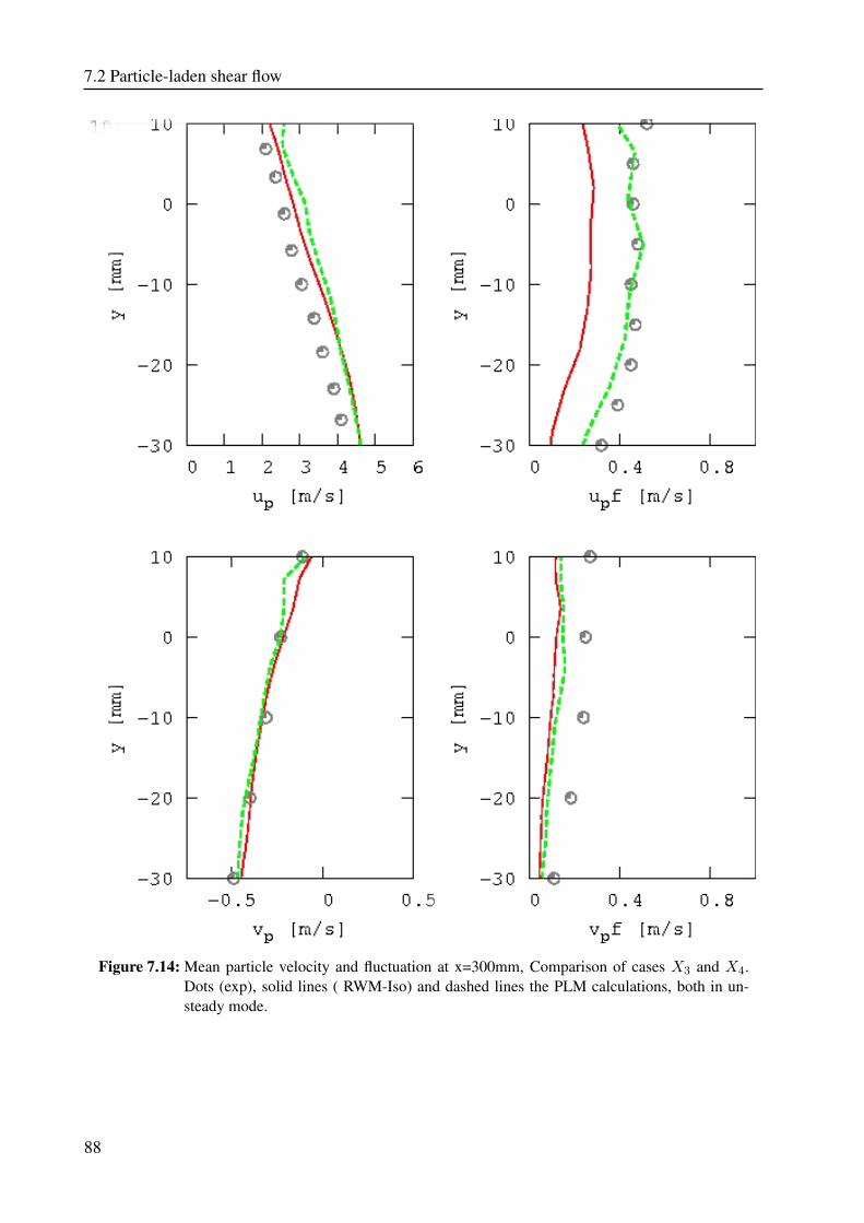
7.2 Particle-laden shear flow
Figure 7.14: Mean particle velocity and fluctuation at x=300mm, Comparison of cases X3 and X4.Dots (exp), solid lines ( RWM-Iso) and dashed lines the PLM calculations, both in un-steady mode.
88
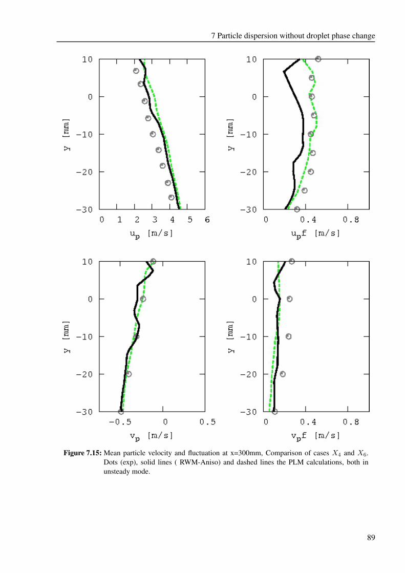
7 Particle dispersion without droplet phase change
Figure 7.15: Mean particle velocity and fluctuation at x=300mm, Comparison of cases X4 and X6.Dots (exp), solid lines ( RWM-Aniso) and dashed lines the PLM calculations, both inunsteady mode.
89
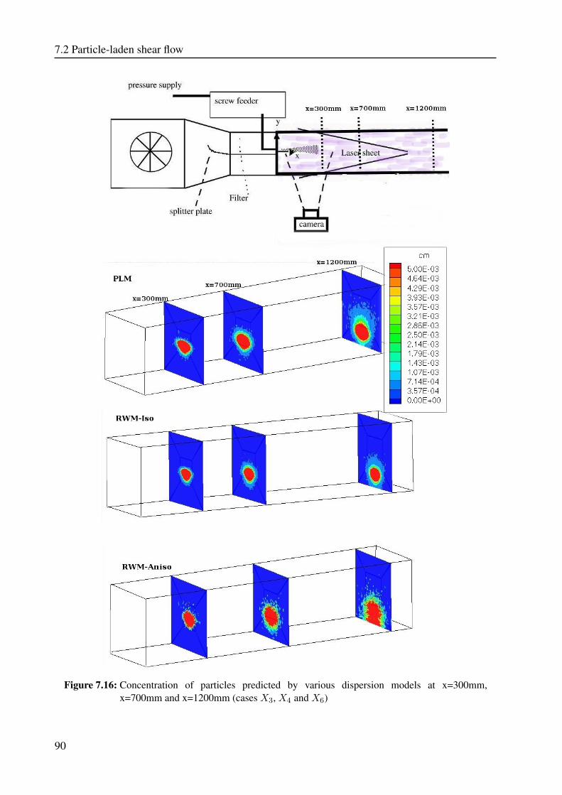
7.2 Particle-laden shear flow
Figure 7.16: Concentration of particles predicted by various dispersion models at x=300mm,x=700mm and x=1200mm (cases X3, X4 and X6)
90
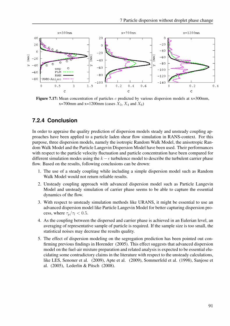
7 Particle dispersion without droplet phase change
Figure 7.17: Mean concentration of particles c predicted by various dispersion models at x=300mm,x=700mm and x=1200mm (cases X3, X4 and X6)
7.2.4 Conclusion
In order to appraise the quality prediction of dispersion models steady and unsteady coupling ap-proaches have been applied to a particle laden shear flow simulation in RANS-context. For thispurpose, three dispersion models, namely the isotropic Random Walk Model, the anisotropic Ran-dom Walk Model and the Particle Langevin Dispersion Model have been used. Their performanceswith respect to the particle velocity fluctuation and particle concentration have been compared fordifferent simulation modes using the k− ε turbulence model to describe the turbulent carrier phaseflow. Based on the results, following conclusions can be drown:
1. The use of a steady coupling while including a simple dispersion model such as RandomWalk Model would not return reliable results.
2. Unsteady coupling approach with advanced dispersion model such as Particle LangevinModel and unsteady simulation of carrier phase seems to be able to capture the essentialdynamics of the flow.
3. With respect to unsteady simulation methods like URANS, it might be essential to use anadvanced dispersion model like Particle Langevin Model for better capturing dispersion pro-cess, where τp/τl < 0.5.
4. As the coupling between the dispersed and carrier phase is achieved in an Eulerian level, anaveraging of representative sample of particle is required. If the sample size is too small, thestatistical noises may decrease the results quality.
5. The effect of dispersion modeling on the segregation prediction has been pointed out con-firming previous findings in Horender (2005). This effect suggests that advanced dispersionmodel on the fuel-air mixture preparation and related analysis is expected to be essential elu-cidating some contradictory claims in the literature with respect to the unsteady calculations,like LES, Senoner et al. (2009), Apte et al. (2009), Sommerfeld et al. (1998), Sanjose etal. (2005), Lederlin & Pitsch (2008).
91

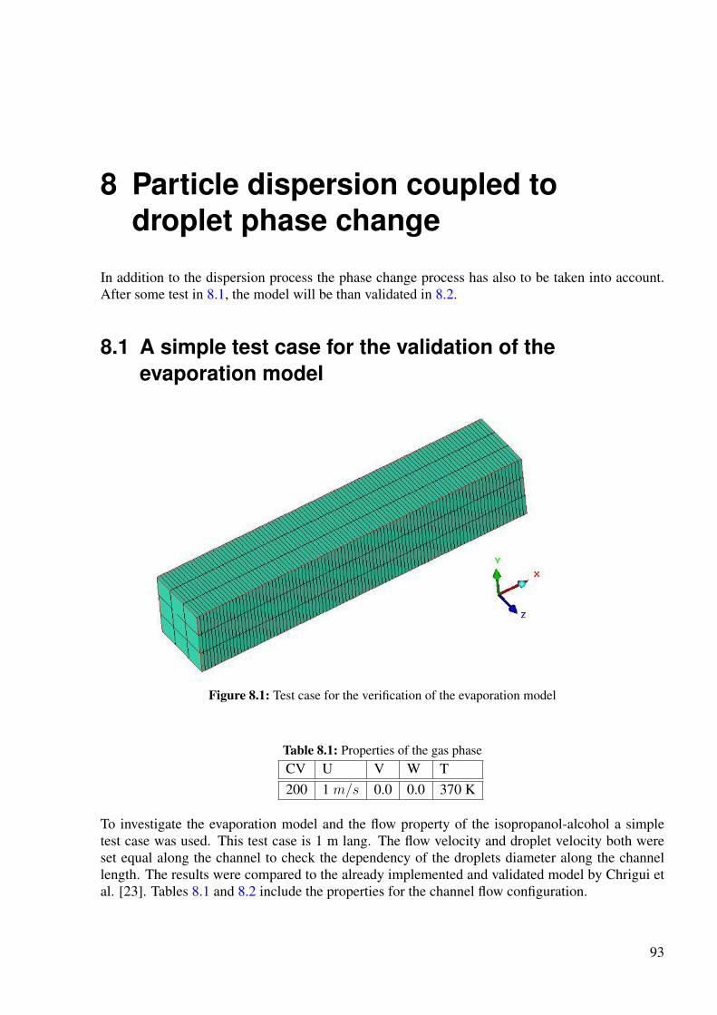
8 Particle dispersion coupled todroplet phase change
In addition to the dispersion process the phase change process has also to be taken into account.After some test in 8.1, the model will be than validated in 8.2.
8.1 A simple test case for the validation of theevaporation model
Figure 8.1: Test case for the verification of the evaporation model
Table 8.1: Properties of the gas phaseCV U V W T200 1 m/s 0.0 0.0 370 K
To investigate the evaporation model and the flow property of the isopropanol-alcohol a simpletest case was used. This test case is 1 m lang. The flow velocity and droplet velocity both wereset equal along the channel to check the dependency of the droplets diameter along the channellength. The results were compared to the already implemented and validated model by Chrigui etal. [23]. Tables 8.1 and 8.2 include the properties for the channel flow configuration.
93
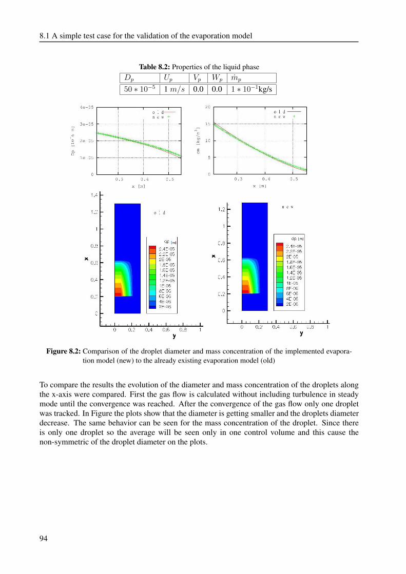
8.1 A simple test case for the validation of the evaporation model
Table 8.2: Properties of the liquid phaseDp Up Vp Wp mp
50 ∗ 10−5 1 m/s 0.0 0.0 1 ∗ 10−1kg/s
Figure 8.2: Comparison of the droplet diameter and mass concentration of the implemented evapora-tion model (new) to the already existing evaporation model (old)
To compare the results the evolution of the diameter and mass concentration of the droplets alongthe x-axis were compared. First the gas flow is calculated without including turbulence in steadymode until the convergence was reached. After the convergence of the gas flow only one dropletwas tracked. In Figure the plots show that the diameter is getting smaller and the droplets diameterdecrease. The same behavior can be seen for the mass concentration of the droplet. Since thereis only one droplet so the average will be seen only in one control volume and this cause thenon-symmetric of the droplet diameter on the plots.
94
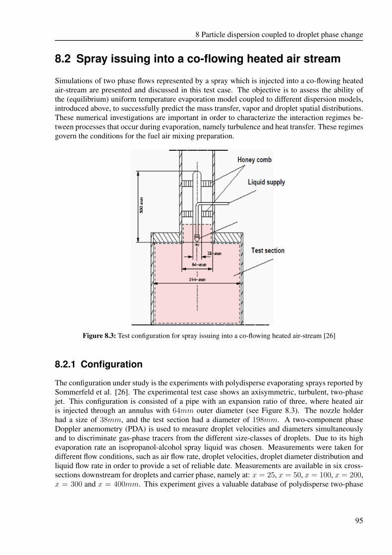
8 Particle dispersion coupled to droplet phase change
8.2 Spray issuing into a co-flowing heated air stream
Simulations of two phase flows represented by a spray which is injected into a co-flowing heatedair-stream are presented and discussed in this test case. The objective is to assess the ability ofthe (equilibrium) uniform temperature evaporation model coupled to different dispersion models,introduced above, to successfully predict the mass transfer, vapor and droplet spatial distributions.These numerical investigations are important in order to characterize the interaction regimes be-tween processes that occur during evaporation, namely turbulence and heat transfer. These regimesgovern the conditions for the fuel air mixing preparation.
Figure 8.3: Test configuration for spray issuing into a co-flowing heated air-stream [26]
8.2.1 Configuration
The configuration under study is the experiments with polydisperse evaporating sprays reported bySommerfeld et al. [26]. The experimental test case shows an axisymmetric, turbulent, two-phasejet. This configuration is consisted of a pipe with an expansion ratio of three, where heated airis injected through an annulus with 64mm outer diameter (see Figure 8.3). The nozzle holderhad a size of 38mm, and the test section had a diameter of 198mm. A two-component phaseDoppler anemometry (PDA) is used to measure droplet velocities and diameters simultaneouslyand to discriminate gas-phase tracers from the different size-classes of droplets. Due to its highevaporation rate an isopropanol-alcohol spray liquid was chosen. Measurements were taken fordifferent flow conditions, such as air flow rate, droplet velocities, droplet diameter distribution andliquid flow rate in order to provide a set of reliable date. Measurements are available in six cross-sections downstream for droplets and carrier phase, namely at: x = 25, x = 50, x = 100, x = 200,x = 300 and x = 400mm. This experiment gives a valuable database of polydisperse two-phase
95
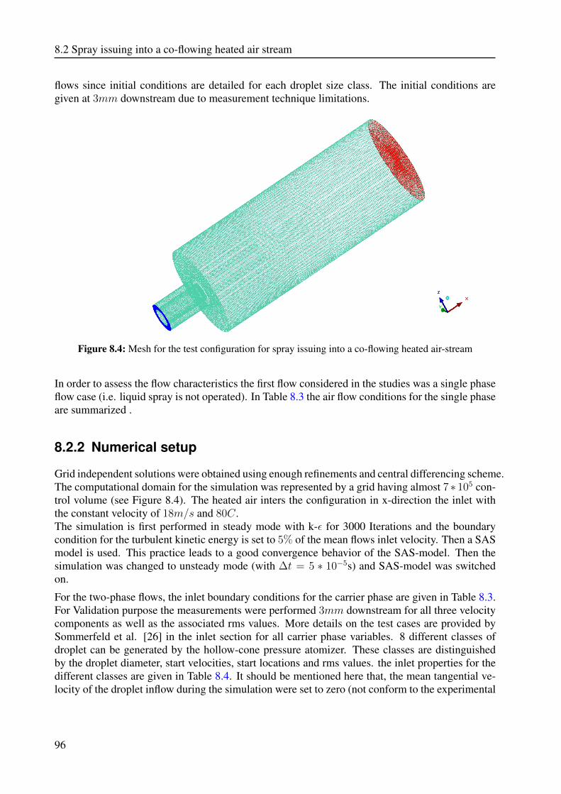
8.2 Spray issuing into a co-flowing heated air stream
flows since initial conditions are detailed for each droplet size class. The initial conditions aregiven at 3mm downstream due to measurement technique limitations.
Figure 8.4: Mesh for the test configuration for spray issuing into a co-flowing heated air-stream
In order to assess the flow characteristics the first flow considered in the studies was a single phaseflow case (i.e. liquid spray is not operated). In Table 8.3 the air flow conditions for the single phaseare summarized .
8.2.2 Numerical setup
Grid independent solutions were obtained using enough refinements and central differencing scheme.The computational domain for the simulation was represented by a grid having almost 7∗ 105 con-trol volume (see Figure 8.4). The heated air inters the configuration in x-direction the inlet withthe constant velocity of 18m/s and 80C.The simulation is first performed in steady mode with k-ε for 3000 Iterations and the boundarycondition for the turbulent kinetic energy is set to 5% of the mean flows inlet velocity. Then a SASmodel is used. This practice leads to a good convergence behavior of the SAS-model. Then thesimulation was changed to unsteady mode (with ∆t = 5 ∗ 10−5s) and SAS-model was switchedon.
For the two-phase flows, the inlet boundary conditions for the carrier phase are given in Table 8.3.For Validation purpose the measurements were performed 3mm downstream for all three velocitycomponents as well as the associated rms values. More details on the test cases are provided bySommerfeld et al. [26] in the inlet section for all carrier phase variables. 8 different classes ofdroplet can be generated by the hollow-cone pressure atomizer. These classes are distinguishedby the droplet diameter, start velocities, start locations and rms values. the inlet properties for thedifferent classes are given in Table 8.4. It should be mentioned here that, the mean tangential ve-locity of the droplet inflow during the simulation were set to zero (not conform to the experimental
96
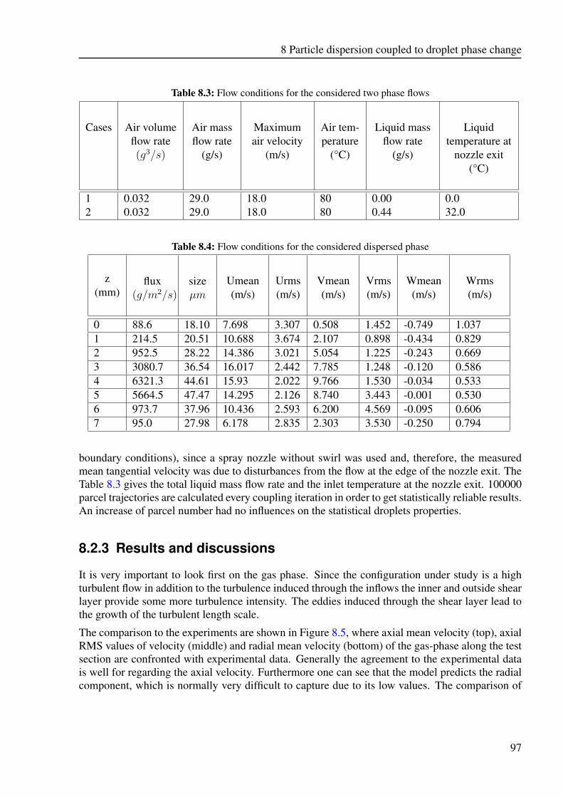
8 Particle dispersion coupled to droplet phase change
Table 8.3: Flow conditions for the considered two phase flows
Cases Air volumeflow rate(g3/s)
Air massflow rate
(g/s)
Maximumair velocity
(m/s)
Air tem-perature
(°C)
Liquid massflow rate
(g/s)
Liquidtemperature at
nozzle exit(°C)
1 0.032 29.0 18.0 80 0.00 0.02 0.032 29.0 18.0 80 0.44 32.0
Table 8.4: Flow conditions for the considered dispersed phase
z(mm)
flux(g/m2/s)
sizeµm
Umean(m/s)
Urms(m/s)
Vmean(m/s)
Vrms(m/s)
Wmean(m/s)
Wrms(m/s)
0 88.6 18.10 7.698 3.307 0.508 1.452 -0.749 1.0371 214.5 20.51 10.688 3.674 2.107 0.898 -0.434 0.8292 952.5 28.22 14.386 3.021 5.054 1.225 -0.243 0.6693 3080.7 36.54 16.017 2.442 7.785 1.248 -0.120 0.5864 6321.3 44.61 15.93 2.022 9.766 1.530 -0.034 0.5335 5664.5 47.47 14.295 2.126 8.740 3.443 -0.001 0.5306 973.7 37.96 10.436 2.593 6.200 4.569 -0.095 0.6067 95.0 27.98 6.178 2.835 2.303 3.530 -0.250 0.794
boundary conditions), since a spray nozzle without swirl was used and, therefore, the measuredmean tangential velocity was due to disturbances from the flow at the edge of the nozzle exit. TheTable 8.3 gives the total liquid mass flow rate and the inlet temperature at the nozzle exit. 100000parcel trajectories are calculated every coupling iteration in order to get statistically reliable results.An increase of parcel number had no influences on the statistical droplets properties.
8.2.3 Results and discussions
It is very important to look first on the gas phase. Since the configuration under study is a highturbulent flow in addition to the turbulence induced through the inflows the inner and outside shearlayer provide some more turbulence intensity. The eddies induced through the shear layer lead tothe growth of the turbulent length scale.
The comparison to the experiments are shown in Figure 8.5, where axial mean velocity (top), axialRMS values of velocity (middle) and radial mean velocity (bottom) of the gas-phase along the testsection are confronted with experimental data. Generally the agreement to the experimental datais well for regarding the axial velocity. Furthermore one can see that the model predicts the radialcomponent, which is normally very difficult to capture due to its low values. The comparison of
97
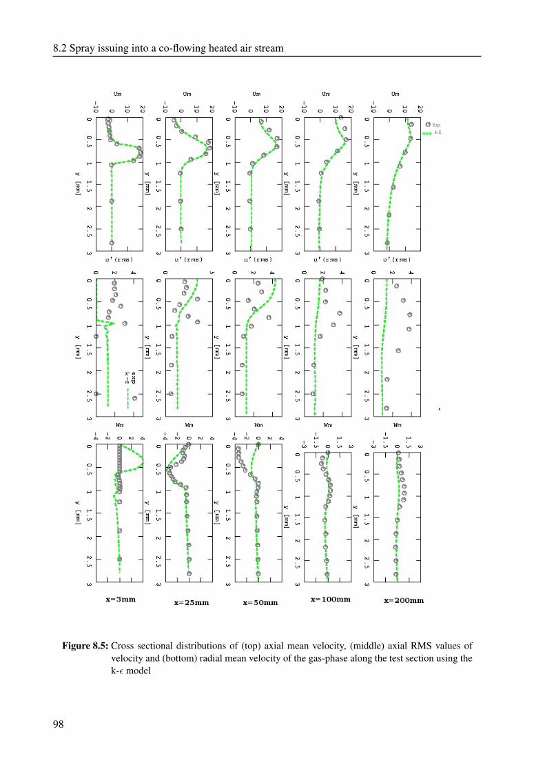
8.2 Spray issuing into a co-flowing heated air stream
Figure 8.5: Cross sectional distributions of (top) axial mean velocity, (middle) axial RMS values ofvelocity and (bottom) radial mean velocity of the gas-phase along the test section using thek-ε model
98
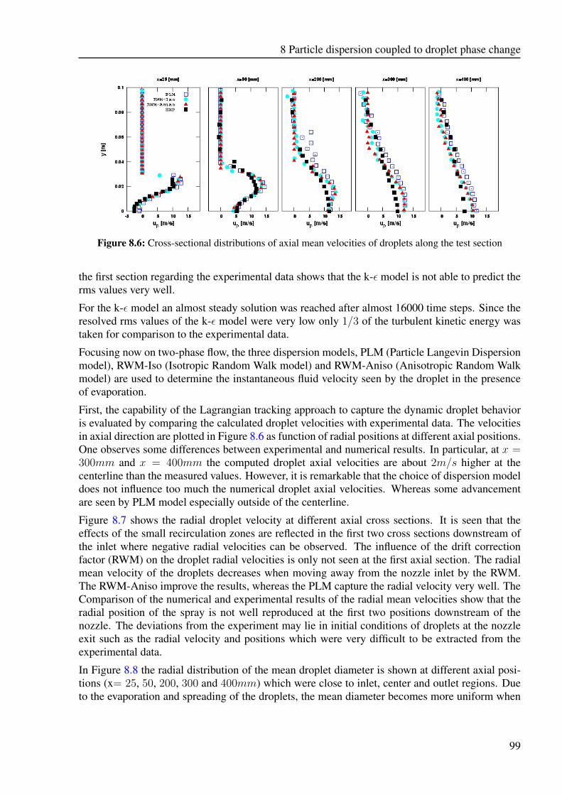
8 Particle dispersion coupled to droplet phase change
Figure 8.6: Cross-sectional distributions of axial mean velocities of droplets along the test section
the first section regarding the experimental data shows that the k-ε model is not able to predict therms values very well.
For the k-ε model an almost steady solution was reached after almost 16000 time steps. Since theresolved rms values of the k-ε model were very low only 1/3 of the turbulent kinetic energy wastaken for comparison to the experimental data.
Focusing now on two-phase flow, the three dispersion models, PLM (Particle Langevin Dispersionmodel), RWM-Iso (Isotropic Random Walk model) and RWM-Aniso (Anisotropic Random Walkmodel) are used to determine the instantaneous fluid velocity seen by the droplet in the presenceof evaporation.
First, the capability of the Lagrangian tracking approach to capture the dynamic droplet behavioris evaluated by comparing the calculated droplet velocities with experimental data. The velocitiesin axial direction are plotted in Figure 8.6 as function of radial positions at different axial positions.One observes some differences between experimental and numerical results. In particular, at x =300mm and x = 400mm the computed droplet axial velocities are about 2m/s higher at thecenterline than the measured values. However, it is remarkable that the choice of dispersion modeldoes not influence too much the numerical droplet axial velocities. Whereas some advancementare seen by PLM model especially outside of the centerline.
Figure 8.7 shows the radial droplet velocity at different axial cross sections. It is seen that theeffects of the small recirculation zones are reflected in the first two cross sections downstream ofthe inlet where negative radial velocities can be observed. The influence of the drift correctionfactor (RWM) on the droplet radial velocities is only not seen at the first axial section. The radialmean velocity of the droplets decreases when moving away from the nozzle inlet by the RWM.The RWM-Aniso improve the results, whereas the PLM capture the radial velocity very well. TheComparison of the numerical and experimental results of the radial mean velocities show that theradial position of the spray is not well reproduced at the first two positions downstream of thenozzle. The deviations from the experiment may lie in initial conditions of droplets at the nozzleexit such as the radial velocity and positions which were very difficult to be extracted from theexperimental data.
In Figure 8.8 the radial distribution of the mean droplet diameter is shown at different axial posi-tions (x= 25, 50, 200, 300 and 400mm) which were close to inlet, center and outlet regions. Dueto the evaporation and spreading of the droplets, the mean diameter becomes more uniform when
99
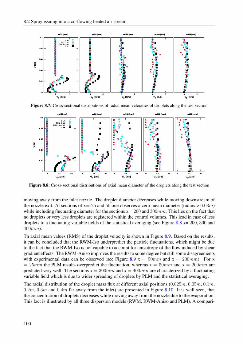
8.2 Spray issuing into a co-flowing heated air stream
Figure 8.7: Cross-sectional distributions of radial mean velocities of droplets along the test section
Figure 8.8: Cross-sectional distributions of axial mean diameter of the droplets along the test section
moving away from the inlet nozzle. The droplet diameter decreases while moving downstream ofthe nozzle exit. At sections of x= 25 and 50 one observes a zero mean diameter (radius > 0.03m)while including fluctuating diameter for the sections x= 200 and 300mm. This lies on the fact thatno droplets or very less droplets are registered within the control volumes. This lead in case of lessdroplets to a fluctuating variable fields of the statistical averaging (see Figure 8.8 x= 200, 300 and400mm).
Th axial mean values (RMS) of the droplet velocity is shown in Figure 8.9. Based on the results,it can be concluded that the RWM-Iso underpredict the particle fluctuations, which might be dueto the fact that the RWM-Iso is not capable to account for anisotropy of the flow induced by sheargradient effects. The RWM-Aniso improves the results to some degree but still some disagreementswith experimental data can be observed (see Figure 8.9 x = 50mm and x = 200mm). For x= 25mm the PLM results overpredict the fluctuation, whereas x = 50mm and x = 200mm arepredicted very well. The sections x = 300mm and x = 400mm are characterized by a fluctuatingvariable field which is due to wider spreading of droplets by PLM and the statistical averaging.
The radial distribution of the droplet mass flux at different axial positions (0.025m, 0.05m, 0.1m,0.2m, 0.3m and 0.4m far away from the inlet) are presented in Figure 8.10. It is well seen, thatthe concentration of droplets decreases while moving away from the nozzle due to the evaporation.This fact is illustrated by all three dispersion models (RWM, RWM-Aniso and PLM). A compari-
100
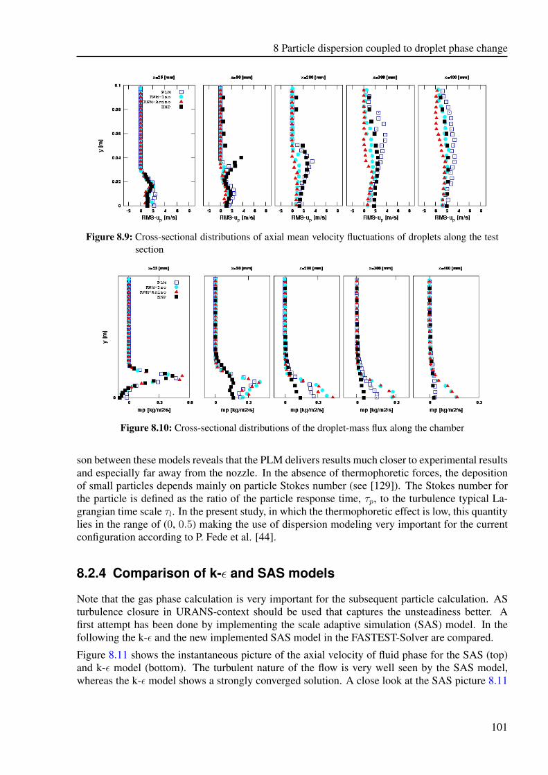
8 Particle dispersion coupled to droplet phase change
Figure 8.9: Cross-sectional distributions of axial mean velocity fluctuations of droplets along the testsection
Figure 8.10: Cross-sectional distributions of the droplet-mass flux along the chamber
son between these models reveals that the PLM delivers results much closer to experimental resultsand especially far away from the nozzle. In the absence of thermophoretic forces, the depositionof small particles depends mainly on particle Stokes number (see [129]). The Stokes number forthe particle is defined as the ratio of the particle response time, τp, to the turbulence typical La-grangian time scale τl. In the present study, in which the thermophoretic effect is low, this quantitylies in the range of (0, 0.5) making the use of dispersion modeling very important for the currentconfiguration according to P. Fede et al. [44].
8.2.4 Comparison of k-ε and SAS models
Note that the gas phase calculation is very important for the subsequent particle calculation. ASturbulence closure in URANS-context should be used that captures the unsteadiness better. Afirst attempt has been done by implementing the scale adaptive simulation (SAS) model. In thefollowing the k-ε and the new implemented SAS model in the FASTEST-Solver are compared.
Figure 8.11 shows the instantaneous picture of the axial velocity of fluid phase for the SAS (top)and k-ε model (bottom). The turbulent nature of the flow is very well seen by the SAS model,whereas the k-ε model shows a strongly converged solution. A close look at the SAS picture 8.11
101
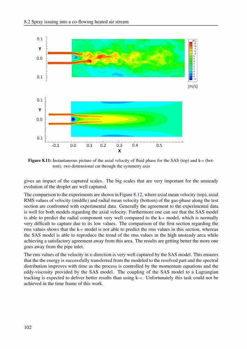
8.2 Spray issuing into a co-flowing heated air stream
Figure 8.11: Instantaneous picture of the axial velocity of fluid phase for the SAS (top) and k-ε (bot-tom). two dimensional cut through the symmetry axis
gives an impact of the captured scales. The big scales that are very important for the unsteadyevolution of the droplet are well captured.
The comparison to the experiments are shown in Figure 8.12, where axial mean velocity (top), axialRMS values of velocity (middle) and radial mean velocity (bottom) of the gas-phase along the testsection are confronted with experimental data. Generally the agreement to the experimental datais well for both models regarding the axial velocity. Furthermore one can see that the SAS modelis able to predict the radial component very well compared to the k-ε model, which is normallyvery difficult to capture due to its low values. The comparison of the first section regarding therms values shows that the k-ε model is not able to predict the rms values in this section, whereasthe SAS model is able to reproduce the trend of the rms values in the high unsteady area whileachieving a satisfactory agreement away from this area. The results are getting better the more onegoes away from the pipe inlet.
The rms values of the velocity in x-direction is very well captured by the SAS model. This ensuresthat the the energy is successfully transferred from the modeled to the resolved part and the spectraldistribution improves with time as the process is controlled by the momentum equations and theeddy-viscosity provided by the SAS model. The coupling of the SAS model to a Lagrangiantracking is expected to deliver better results than using k–ε. Unfortunately this task could not beachieved in the time frame of this work.
102
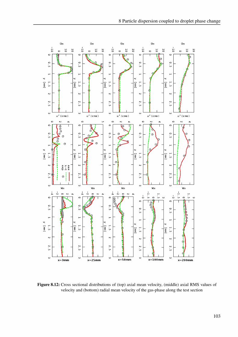
8 Particle dispersion coupled to droplet phase change
Figure 8.12: Cross sectional distributions of (top) axial mean velocity, (middle) axial RMS values ofvelocity and (bottom) radial mean velocity of the gas-phase along the test section
103

8.2 Spray issuing into a co-flowing heated air stream
8.2.5 Conclusion
In this section different dispersion models were used in combinations with the uniform temperatureevaporation model to investigate the spray and droplet properties under non isothermal and nonreacting conditions. The results show that the PLM is able to achieve better results with respectto radial mean velocities, mean diameter and axial mean velocity fluctuations of droplets. So thesimulations have shown that the PLM model agreed very well with the experimental measurementof the droplet mass flux in particular in upper sections. This means that the consideration of anadvanced dispersion model like PLM accounts well for anisotropic turbulence and vortex structuresinherent to complex turbulent two phase flows.
In regard to the used turbulence models one can say that the agreement to the experimental datais well for both models regarding the axial velocity. The radial component is reproduced by SASmodel very well compared to the k-ε model, which is normally very difficult to capture due to itslow values. Rms values with SAS are in a satisfactory agreement away from the inlet.
The rms values of the velocity in x-direction is very well captured by the SAS model.
The coupling of the SAS model to the dispersed phase is still work in progress, so that the nextstep is to compare the two phase flow results for k-ε model and SAS model.
104
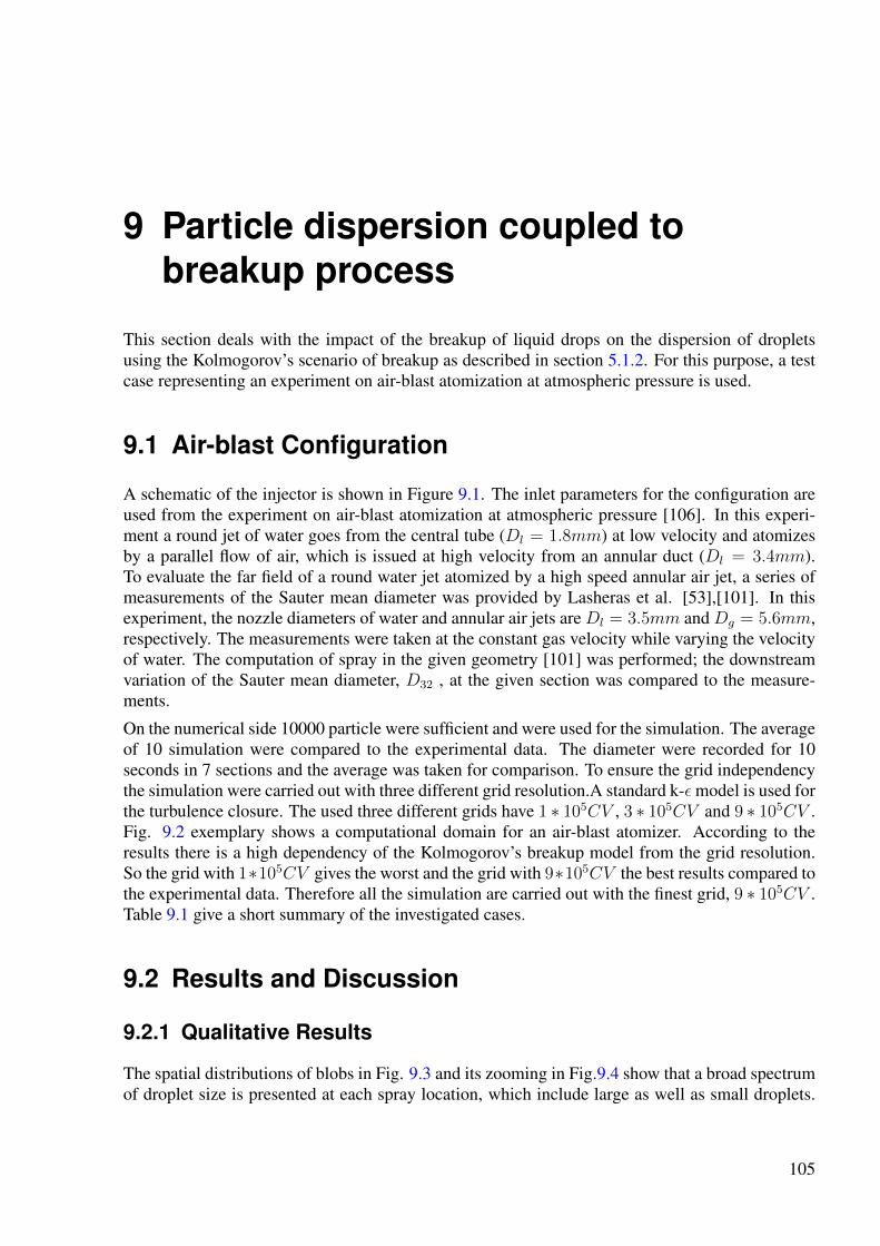
9 Particle dispersion coupled tobreakup process
This section deals with the impact of the breakup of liquid drops on the dispersion of dropletsusing the Kolmogorov’s scenario of breakup as described in section 5.1.2. For this purpose, a testcase representing an experiment on air-blast atomization at atmospheric pressure is used.
9.1 Air-blast Configuration
A schematic of the injector is shown in Figure 9.1. The inlet parameters for the configuration areused from the experiment on air-blast atomization at atmospheric pressure [106]. In this experi-ment a round jet of water goes from the central tube (Dl = 1.8mm) at low velocity and atomizesby a parallel flow of air, which is issued at high velocity from an annular duct (Dl = 3.4mm).To evaluate the far field of a round water jet atomized by a high speed annular air jet, a series ofmeasurements of the Sauter mean diameter was provided by Lasheras et al. [53],[101]. In thisexperiment, the nozzle diameters of water and annular air jets are Dl = 3.5mm and Dg = 5.6mm,respectively. The measurements were taken at the constant gas velocity while varying the velocityof water. The computation of spray in the given geometry [101] was performed; the downstreamvariation of the Sauter mean diameter, D32 , at the given section was compared to the measure-ments.
On the numerical side 10000 particle were sufficient and were used for the simulation. The averageof 10 simulation were compared to the experimental data. The diameter were recorded for 10seconds in 7 sections and the average was taken for comparison. To ensure the grid independencythe simulation were carried out with three different grid resolution.A standard k-εmodel is used forthe turbulence closure. The used three different grids have 1 ∗ 105CV , 3 ∗ 105CV and 9 ∗ 105CV .Fig. 9.2 exemplary shows a computational domain for an air-blast atomizer. According to theresults there is a high dependency of the Kolmogorov’s breakup model from the grid resolution.So the grid with 1∗105CV gives the worst and the grid with 9∗105CV the best results compared tothe experimental data. Therefore all the simulation are carried out with the finest grid, 9 ∗ 105CV .Table 9.1 give a short summary of the investigated cases.
9.2 Results and Discussion
9.2.1 Qualitative Results
The spatial distributions of blobs in Fig. 9.3 and its zooming in Fig.9.4 show that a broad spectrumof droplet size is presented at each spray location, which include large as well as small droplets.
105
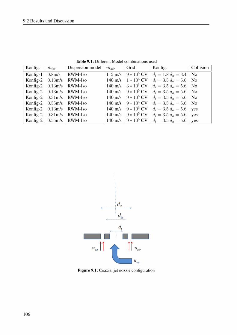
9.2 Results and Discussion
Table 9.1: Different Model combinations usedKonfig. mliq Dispersion model mair Grid Konfig. CollisionKonfig-1 0.8m/s RWM-Iso 115 m/s 9 ∗ 105 CV di = 1.8 da = 3.4 NoKonfig-2 0.13m/s RWM-Iso 140 m/s 1 ∗ 105 CV di = 3.5 da = 5.6 NoKonfig-2 0.13m/s RWM-Iso 140 m/s 3 ∗ 105 CV di = 3.5 da = 5.6 NoKonfig-2 0.13m/s RWM-Iso 140 m/s 9 ∗ 105 CV di = 3.5 da = 5.6 NoKonfig-2 0.31m/s RWM-Iso 140 m/s 9 ∗ 105 CV di = 3.5 da = 5.6 NoKonfig-2 0.55m/s RWM-Iso 140 m/s 9 ∗ 105 CV di = 3.5 da = 5.6 NoKonfig-2 0.13m/s RWM-Iso 140 m/s 9 ∗ 105 CV di = 3.5 da = 5.6 yesKonfig-2 0.31m/s RWM-Iso 140 m/s 9 ∗ 105 CV di = 3.5 da = 5.6 yesKonfig-2 0.55m/s RWM-Iso 140 m/s 9 ∗ 105 CV di = 3.5 da = 5.6 yes
Figure 9.1: Coaxial jet nozzle configuration
106
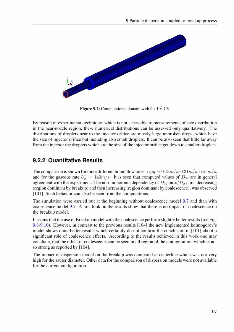
9 Particle dispersion coupled to breakup process
Figure 9.2: Computational domain with 9 ∗ 105 CV
By reason of experimental technique, which is not accessible to measurements of size distributionin the near-nozzle region, these numerical distributions can be assessed only qualitatively. Thedistributions of droplets near to the injector orifice are mostly large unbroken drops, which havethe size of injector orifice but including also small droplets. It can be also seen that little far awayfrom the injector the droplets which are the size of the injector orifice get down to smaller droplets.
9.2.2 Quantitative Results
The comparison is shown for three different liquid flow rates: Uliq = 0.13m/s; 0.31m/s; 0.55m/s,and for the gaseous rate Ug = 140m/s. It is seen that computed values of D32 are in generalagreement with the experiment. The non-monotonic dependency of D32 on x/Dg , first decreasing(region dominant by breakup) and then increasing (region dominant by coalescence), was observed[101]. Such behavior can also be seen from the computations.
The simulation were carried out at the beginning without coalescence model 9.7 and than withcoalescence model 9.7. A first look on the results show that there is no impact of coalescence onthe breakup model.
It seems that the use of Breakup model with the coalescence perform slightly better results (see Fig.9.8-9.10). However, in contrast to the previous results [104] the new implemented kolmogorov’smodel shows quite better results which certainly do not confirm the conclusion in [101] about asignificant role of coalescence effects. According to the results achieved in this work one mayconclude, that the effect of coalescence can be seen in all region of the configuration, which is notso strong as reported by [104].
The impact of dispersion model on the breakup was compared at centerline which was not veryhigh for the sauter diameter. Other data for the comparison of dispersion models were not availablefor the current configuration.
107
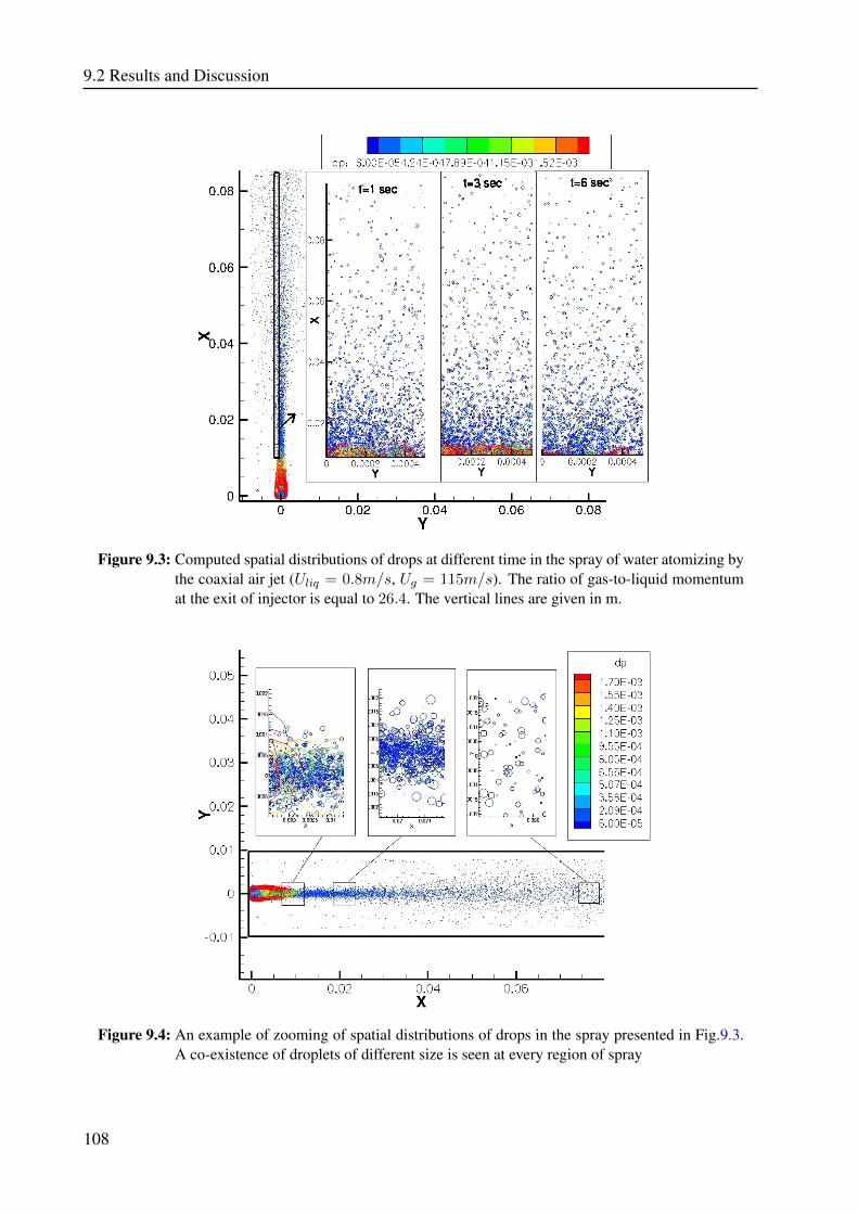
9.2 Results and Discussion
Figure 9.3: Computed spatial distributions of drops at different time in the spray of water atomizing bythe coaxial air jet (Uliq = 0.8m/s, Ug = 115m/s). The ratio of gas-to-liquid momentumat the exit of injector is equal to 26.4. The vertical lines are given in m.
Figure 9.4: An example of zooming of spatial distributions of drops in the spray presented in Fig.9.3.A co-existence of droplets of different size is seen at every region of spray
108
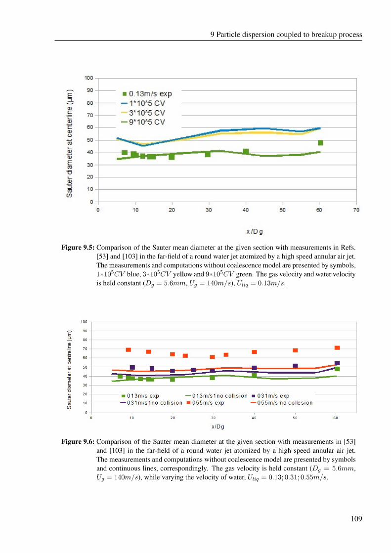
9 Particle dispersion coupled to breakup process
Figure 9.5: Comparison of the Sauter mean diameter at the given section with measurements in Refs.[53] and [103] in the far-field of a round water jet atomized by a high speed annular air jet.The measurements and computations without coalescence model are presented by symbols,1∗105CV blue, 3∗105CV yellow and 9∗105CV green. The gas velocity and water velocityis held constant (Dg = 5.6mm, Ug = 140m/s), Uliq = 0.13m/s.
Figure 9.6: Comparison of the Sauter mean diameter at the given section with measurements in [53]and [103] in the far-field of a round water jet atomized by a high speed annular air jet.The measurements and computations without coalescence model are presented by symbolsand continuous lines, correspondingly. The gas velocity is held constant (Dg = 5.6mm,Ug = 140m/s), while varying the velocity of water, Uliq = 0.13; 0.31; 0.55m/s.
109
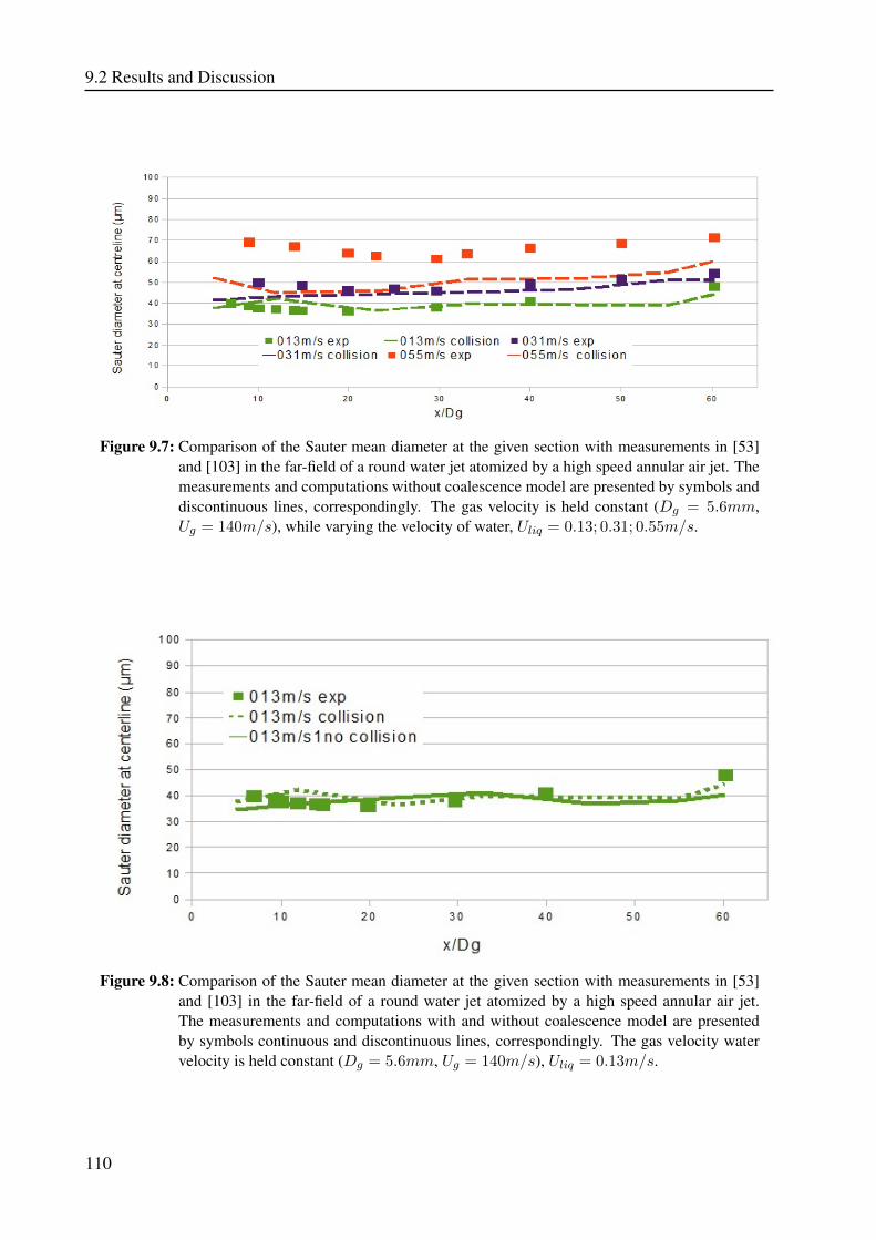
9.2 Results and Discussion
Figure 9.7: Comparison of the Sauter mean diameter at the given section with measurements in [53]and [103] in the far-field of a round water jet atomized by a high speed annular air jet. Themeasurements and computations without coalescence model are presented by symbols anddiscontinuous lines, correspondingly. The gas velocity is held constant (Dg = 5.6mm,Ug = 140m/s), while varying the velocity of water, Uliq = 0.13; 0.31; 0.55m/s.
Figure 9.8: Comparison of the Sauter mean diameter at the given section with measurements in [53]and [103] in the far-field of a round water jet atomized by a high speed annular air jet.The measurements and computations with and without coalescence model are presentedby symbols continuous and discontinuous lines, correspondingly. The gas velocity watervelocity is held constant (Dg = 5.6mm, Ug = 140m/s), Uliq = 0.13m/s.
110
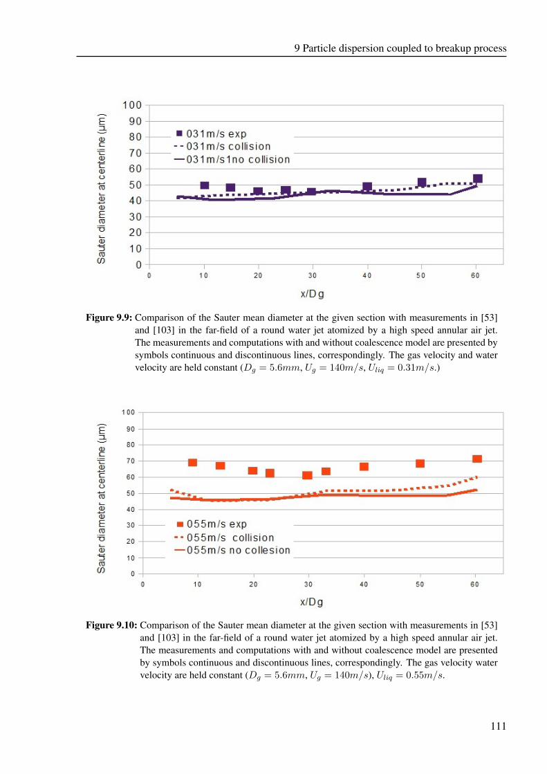
9 Particle dispersion coupled to breakup process
Figure 9.9: Comparison of the Sauter mean diameter at the given section with measurements in [53]and [103] in the far-field of a round water jet atomized by a high speed annular air jet.The measurements and computations with and without coalescence model are presented bysymbols continuous and discontinuous lines, correspondingly. The gas velocity and watervelocity are held constant (Dg = 5.6mm, Ug = 140m/s, Uliq = 0.31m/s.)
Figure 9.10: Comparison of the Sauter mean diameter at the given section with measurements in [53]and [103] in the far-field of a round water jet atomized by a high speed annular air jet.The measurements and computations with and without coalescence model are presentedby symbols continuous and discontinuous lines, correspondingly. The gas velocity watervelocity are held constant (Dg = 5.6mm, Ug = 140m/s), Uliq = 0.55m/s.
111
9.3 Conclusion
9.3 Conclusion
In this section the stochastic model of drops air-blast breakup, Kolmogorov´s model, was pre-sented and validated. The computations were performed for two configurations. The first oneshowed quantitative results , which confirm the existence of a broad spectrum of droplet size ateach spray location. The computations on the second configuration were performed for differentliquid inlet velocities. The downstream Sauter mean diameter was compared to the far field sprayexperiment. The simulation results were in a good agreement with experimental data. Like theexperimental observation the sauter mean diameter first decreased and then increased in the down-stream direction. Opposite to finding in [104] the effect of coalescence was not very strong at thebeginning as it was claimed as due to the existing two regions dominant by coalescence (at thebeginning) and breakup (at the end). The calculation shows that in fact the effect of coalescenceand breakup exist in every region of the spray. The impact of dispersion model on the breakupwas compared at centerline which was not very high for the sauter diameter. Other data for thecomparison of dispersion models were not available for the current configuration.
112
10 Summary and Outlook
Following the E-L (Eulerian Lagrangian) context, the present work aimed at studying the effectof dispersion modeling on multiphase flow properties for statistically unsteady flows. For thispurpose, the study has included the essential processes that may be impacted by the turbulentparticle dispersion, like
1. break up process along with four-way coupling
2. phase change phenomena
3. interaction between phases
Especially, the unsteady numerical coupling within URANS context has been adapted to capturethe unsteadiness of the two-phase flows.
Three dispersion models, namely RWM-Iso, RWM-Aniso and PLM, were integrated and com-pared. Three configurations have been used for model appraisal with respect to their ability toretrieve unsteady behavior of the turbulent dispersion. In a vertical simple channel flow 7.1, wherethe unsteady effects are not very high for the near field, all three models achieved comparableresults. In the far field PLM provided better results in regard to the particle velocity fluctuation,whereas the other two models show a constant particle velocity fluctuation especially in the centerregion.
For the shear layer configuration (see 7.2) where the unsteady effects are higher than in the verticalchannel flow the RWMs underpredicte the particle velocity fluctuation too much compared to thePLM.
Based on these results, following conclusions can be drawn:
1. The use of a steady numerical coupling while including a simple dispersion model such asRandom Walk Model would not return reliable results.
2. Unsteady coupling approach with advanced dispersion model such as Particle LangevinModel and unsteady simulation of carrier phase seems to be able to capture the essentialdynamics of the flow.
3. With respect to unsteady simulation methods like URANS, it might be essential to use anadvanced dispersion model like Particle Langevin Model for better capturing dispersion pro-cess when τp/τl < 0.5 in accordance to [44].
4. As the coupling between the disperse and carrier phase is achieved in an Eulerian level, anaveraging of representative sample of particle is required. If the sample size is too small, thestatistical noises may decrease the results quality.
5. The effect of dispersion modeling on the segregation prediction has been pointed out con-firming previous findings by [13]. This effect suggests that advanced dispersion model onthe fuel-air mixture preparation and related analysis is expected to be essential elucidating
113
some contradictory claims in the literature with respect to the unsteady calculations, likeLES, [36], [37], [43], [41].
In order to assess the ability of the equilibrium uniform temperature evaporation models to suc-cessfully predict the mass transfer and vapor distributions, the test case experimentally investigatedby Sommerfeld et al. [26], which consists of spray issuing into a co-flowing heated air stream, hasbeen numerically studied. A systematical study of different dispersion models and their influenceon mass transfer has been satisfactory carried out (see 8.2).
The results show that the PLM is able to achieve better results with respect to radial mean ve-locities, mean diameter and axial mean velocity fluctuations of droplets. So the simulations haveshown that the PLM model allows for achieving results that agree very well with the experimentalmeasurement of the droplet mass flux in particular in upper sections. This means that the con-sideration of the advanced dispersion models like PLM enables to account well for anisotropicturbulence as well as vortex structures inherent to complex turbulent two phase flows.
In order to better capture unsteady dynamics using RANS calculation, a modified SAS model (see8.2) has been adopted. Comparisons of k-ε and SAS model (see 8.2) results show huge differenceswith respect to the fluctuating velocity in axial direction for the spray case issuing into a co-flowingheated air-stream. With regard to experimental data for the fluctuating velocity the SAS model isable to capture this behavior very well especially far away from the expansion, whereas k-ε modelshows a very raph tendency in the near expansion region and underpredicts very strongly the faraway region. The coupling of SAS model with the dispersed phase solver, LAG3D, is left for thefuture work.
The first step for representing inflow boundary conditions for the dispersed phase in vicinity ofparticle injection nozzle is achieved using stochastic model of drops air-blast breakup followingthe Kolmogorov´s model. Two different configurations of an air-blast atomizer were investigated.For the first configuration qualitative results showed good agreement with the experimental datawith respect to coexistence of large and small droplets.In the second configuration, the effect of different liquid inlet velocities were investigated. Thedownstream Sauter mean diameter was compared with the far field spray experiment. The compu-tational values reproduce in a good agreement the experimental data: the sauter mean diameter firstdecreases and then increases in the downstream direction. The effect of coalescence was found notvery strong at the beginning as it was claimed in other papers by existing of two regions dominateby coalescence (at the beginning) and breakup (at the end). Here the calculation showed that theeffect of coalescence and breakup exist in every region of the spray.
Due to the lack of experimental data for the above configurations, the influence of dispersion mod-els on the breakup could not be investigated. In a future work the validation of the breakup modelin a complex configuration has to be accomplished.
114
11 Zusammenfassung und Ausblick
In der vorliegenden Arbeit wurden Effekte der Dispersion im Euler-Lagrange Kontext in Bezugauf Mehrphasenströmung untersucht. Hierbei wurde besonderes Augenmerk auf
1. Breakup Prozess sowie vierwege Kopplung
2. Verdampfung
3. Interaktion zwischen den Phasen
gelegt. Die Rechnungen wurden im URANS Kontext mit instationärer Kopplung durchgeführt.
Dabei wurden 3 Dispersionsmodelle, RWM-Iso, RWM-Aniso und PLM, zusammengefasst undmiteinander verglichen. Für den Vergleich wurden 3 Konfiguration herangezogen, um die Modellein unterschiedlichen instationäre Intensitäten zu testen und zu vergleichen.
Die erste Konfiguration war ein Vertikal Kanal, wo die instationäre Effekte vergleichsweise niedrigwaren. Der Vergleich von berechneten und experimentellen Daten für Partikelgeschwindigkeitund Partikelgeschwindigkeitsfluktuationen im Inlet-Bereich der Konfiguration zeigte für alle dreiModelle gleich gute Übereinstimmung. Weit weg von dem Inlet-Bereich leistete PLM bessereÜbereinstimmung mit den experimentellen Daten. Die RWMs lieferten dagegen in diesem Bere-ich konstante Fluktuationen.
Für die Shear-Layer Konfiguration waren die RWMs Ergebnisse für die Partikelgeschwindigkeits-fluktuationen sehr niedrig im Vergleich zu den experimentell ermittelten Partikelgeschwindigkeits-fluktuationen.Da die instationäre Effekte in dieser Konfiguration höher im Vergleich zu dem Vertikal-Kanalwaren, wurde die turbulente kinetische Energie modifiziert, indem auch die gelöste Strukturen zudem turbulenten kinetischen Energie hinzuaddiert wurden. Bezogen auf die Ergebnisse folgendeRückschlüsse könnten gezogen werden:
1. Eine stationäre Kopplung mit einem einfachen Dispersionsmodell, z.B. RWM, führt nichtzu verlässlichen Ergebnissen.
2. Instationärer Kopplung mit einem fortgeschrittenen Dispersionsmodell, PLM, und insta-tionäre Berechnung erfasst die grundlegende Dynamik der Strömung.
3. In instationärer Rechnung wie URANS, ist es sinnvoll ein fortgeschrittenes Dispersionsmod-ell, wie PLM zu verwenden, um Partikeldispersion besser zu simulieren, vor allem wennτp/τl < 0.5 (siehe [44]).
4. Die Anzahl der Partikeln/Tropfen ist sehr wichtig für die Berechnung. Um statistisch zuver-lässige Ergebnisse zu bekommen, muss die Anzahl der Tropfen/Partikeln sinnvoll gewähltwerden.
115
5. Dispersion spielt ebenfalls eine große Rolle bei der Segregationsvorhersage und bestätigtdie Ergebnisse im [13]. Die Verwendung von einfachen Dispersionsmodelle für Öl-Luft-Gemische führt zu unrealistischer Ansammlung von Tropfen/Partikeln [36], [37], [43], [41].
Um die Dispersionsmodelle im Falle von Verdampfung miteinander zu vergleichen, wurde dasEquilibrium-Uniform-Temperature Verdampfungsmodell implementiert. Für die Untersuchungwurde eine Konfiguration von Sommerfeld [26] gewählt.
Die Berechnung von Verdampfung mit dem PLM zeigte eine bessere Übereinstimmung mit den ex-perimentellen Daten in Bezug auf radiale mittlere Tropfengeschwindigkeit, mittlere Tropfendurchmesserund Tropfen mittlere axiale Geschwindigkeitsfluktuationen. Die Ergebnisse bestätigten, dass dasPLM gute Anisotropie und Vortex Strukturen abbilden kann.
Um mehr Instationarität im RANS-Kontext zu bekommen, wurde eine modifizierte SAS Mod-ell (siehe 8.2) adaptiert und für die Berechnung der Gasphase in der Verdampfungskonfigurationeingesetzt. Der Vergleich von SAS Modell und k-ε mit den experimentellen Daten zeigte (siehe8.2), dass die axiale Geschwindigkeitsfluktuation mit dem SAS Model gut prädektiert wird, wobeidas k-ε Modell eine sehr grobe Tendenz der Geschwindigkeitsfluktuationen vorhersagt.
Insbesondere weit weg vom Inlet-Bereich werden die Geschwindigkeitsfluktuationen mit dem k-εModell stark unterpredektiert. Die Kopplung von SAS Modell mit der dispersen Phase ist nochnicht abgeschlossen und wird als nächster Schritt definiert.
Ferner wurde ein stochastisches Breakupmodell, das Kolmogorov’s Model, implementiert und anzwei experimentell untersuchten Airblast Atomizer validiert. In der ersten Konfiguration wurdeparallel zu den experimentellen Untersuchung bestätigt, dass in allen Regionen der Konfigurationgroße und kleine Tropfen nebeneinander existieren.In der zweiten Konfiguration wurde der Tropfen-Sauter-Durchmesser mit den experimentell er-mittelten Tropfen-Sauter-Durchmesser verglichen. Der Vergleich zeigte sehr gute Übereinstim-mung. Hierbei wurde auch der Einfluss von Koaleszenz untersucht. Im Gegensatz zu früherenUntersuchungen wurde festgestellt, dass der Einfluss von Koaleszenz nicht sehr groß ist. Fernerwurde herausgefunden, dass Koaleszenz nicht nur in bestimmten Regionen auftritt, sondern über-all auftreten kann.
Mit den vorhandenen experimentellen Daten konnte der Einfluss von Dispersionsmodell auf demBreakupmodell nicht festgestellt werden. Als Ausblick ist es Interessant, das Breakupmodell,Kolmogorov’s Model, für eine komplexe Konfiguration zu berechnen und mit experimentellenDaten zu vergleichen.
116
Bibliography
[1] Core,J.-L. Estivalezes, S. Vincent, O. Simonin, S. Glockner, (2009): Simulation of a flu-idized bed using a hybrid Eulerian Lagrangian method for particle tracking, to appear inNotes on Numerical Fluid Mechanics and Multidisciplinary Design. 2, 3
[2] Sadiki A., Chrigui M., Janicka J. and Maneshkarimi M. R. (2005): modeling and Simulationof effects of turbulence on vaporization, mixing and combustion of liquid fuel sprays, Journalof Flow, Turbulence and Combustion, 2005. 1, 9, 29
[3] Lars Davidson (2006): Unsteady RANS, MTF270 Turbulence Modelling
[4] Tian, L., & Ahmadi, G. (2007) Particle deposition in turbulent duct flows-comparisons ofdifferent model predictions. journal of Aerosol Science, 38, 377–397 (2007).
[5] Parker, Foat, & Preston, (2008): Towards quantitative prediction of aerosol deposition fromturbulent flows journal of Aerosol Science,39, 99–112. 2, 3
[6] Zahmatkesh, I. (2008): On the importance of thermophoresis and Brownian diffusion forthe deposition of micro- and nanoparticles. International Communications in Heat and MassTransfer, 35, 369–375 (1995). 3
[7] Zhang, Z., & Chen. Q. (2009): Prediction of particle deposition onto indoor surfaces byCFD with a modified Lagrangian method.,43, 319–328 (1995).
[8] Cheng, Y. s.(2003): Aerosol deposition in the extrathoracic region.,37, 659–671.2
[9] Matida, E. A., Finlay, W. H., Lange, C. F., & Grgic, B. (2004): Improved numerical simu-lation of aerosol deposition in an idealized mouth-throat. . Journal of Aerosol Science, 35,1–19 2, 3
[10] Shi, H., Kleinstreuer, C., A-Zhang, Z. (2008): Dilute suspension flow with nanoparticledeposition in a representative nasal airway model. Physics of Fluids, 20, 013301.
[11] Pope, S. (1994): Lagrangian pdf methods for turbulent flows.Annu. Rev. Fluid Mech., , 26,23–62 23
[12] Pope, S. b., (2000): Turbulent Flows.. Cambridge University Press, Cambridge, UnitedKingdom. ISBN 52159886., 494-505 3
[13] Horender, S. (2005): Modeling of the vortex-structure in a particle-laden mixing-layer.ASME Fluid Engineering Division Summer Meeting and Exhibition Houston, TX,USA, (2005). 2, 4, 5, 41, 82, 83, 85, 91, 113, 116
117
Bibliography
[14] Minier, J.-P., (1999): Closure proposals for the langevin equation model in lagrangian two-phase flow modelling, In Proceedings of the 3rd ASME/JSME Joint Fluids EngineeringConference. 5
[15] E. Peirano, S. Chibbaro, J.Pozorski, J.-P. Minier (2005): Mean-field/PDF numerical ap-proach for polydispersed turbulent two-phase flows, 37, 659–671. Progress in Energy andCombustion Science, 32, 315–371 (2005). 3, 4, 5, 42
[16] Nomura, H.,Hayasaki, M., Ujiie, Y. (2007): Effects of fine fuel particles on a lminar flamestabilized in a partially prevaporized spray stream.. Proc. Combus. Inst. 31(2), 2265-2272.9
[71] Berlemont, A., Grancher, M.S., Gouesbet, G. (1995): Heat and mass transfer couplingbetween vaporizing particles and turbulence using a Lagrangian approach.. J.Heat MassTransf.38, 3023-3034 3, 47
[18] Kohnen, G., Rüger, M., Sommerfeld, M. (1994): Convergence behavior for numerical cal-culations by the Euler/Lagrange method for strongly coupled phases.. FED-Vol 185, Nu-merical method in Multiphases Flows. ASME, Houston Texas . 4, 5, 28, 70, 73
[19] Melheim, J., Horender, S., sommerfeld, M. (2005):Modeling of the vortex-structure in aparticle laden mixing-layer.. In: Proceeding of FEDSM 2005, ASME 2005, Houston, 19-23. 3, 28, 43
[20] Crowe, C.T., Troutt, T.R., Chung, J.N. (1996):Numerical models for Two-phase turbulentflows.. Ann. Rev. Fluid Mech 28,11-43. 3, 29, 72, 73
[21] Crowe, C.T., Troutt, T.R., Chung, J.N. (1998): Lagrangian stochastic modeling of turbu-lent flows. Advances in Turbulence Modeling. Von Karmon Institute for Fluid Dynamics,Belgium 3
[22] Bart Merci, Dirk Roekaerts, Amsini Sadiki (2011): Experiments and Numerical Simulationsof Diluted spray turbulent combustion.. Proceedings of the 1st international workshop onturbulent spray combustion 78-79 3, 4, 5, 9
[23] Chrigui, M., Ahmadi, G., Sadiki, A.(2004):Study on interaction in spray between evaporat-ing particles and turbulence using second-order turbulence RANS models and a Lagrangianapproach..Prog. Comput. Fluid Dyn.4(3-5), 162-174 29, 43, 46, 70, 71, 72, 73, 93, 127
[24] Ahmadi, G., Cao,J., Schneider, L., Sadiki, A. (2006): A thermodynamically formulation forchemically active multiphase turbulent flows.. Int. J. Eng. Sci. 44, 699–720. 29, 71, 72
[25] Lain, S., Sommerfeld, M. (2003): Turbulence modulation in dispersed two-phase flow ladenwith solids from a Lagrangian perspective.. Int. J. Heat Fluid Flow, 24, 616–625. 29, 43,72, 73, 74
[26] Sommerfeld, M., Qiu, H.H., Reuger, M., Kohnen, G., Spies, P.J., Meuller, D.,(1993): Sprayevaporation in turbulent flow. Proceedings of the 2nd Int. Symp. on Engineering TurbulentModeling and Measurements, Florence, Italy, 31 May untel 2 june, pp. 932-945.
[27] Balachandar, S., Eaton, J.K. (2010):Turbulent dispersed multiphase flows..Annu. Rev. FluidMech., 42, 111–133. 95, 96, 114, 116, 128
118
Bibliography
[28] Tanaka, T., Eaton, J.K. (2008):Classification of turbulence modification by dispersedspheres using a novel dimensionless number..Phys. Rev. Lett. 11, 114502 . 29
[29] Beishuizen, N.A., Naud, B., roekaerts, D.J.E.M. (2007): Evaluation of a modified Reynoldsstress model for turbulent dispersed two-phase flows including two-way coupling..Flow Tur-bul. Combust. 79(3), 321-341 72
[30] Sadiki, A. (2005): Extended thermodynamics as modeling tool of turbulence fluid flows..Trends in Applications of Mathematics to Mechanics, pp. 451-462, Shaker Verlag, Aachen72
[31] Groh, B., Sadiki, A., Janicka, J. (2004): Large eddy simulation of particle-laden verticalchannel flow under consideration of a consistent modeling of turbulence modulation.. In:Proceedings of the 3rd International Symposium on Two-Phase Flow Modeling and Exper-imentation, Pisa, Italy. 72
[32] Walklate, P.J. (1995): A Markov-chain partilce dispersion model based on air flow data:extension to large water particles. Bound-Lay. Meteorol. 37, 313–318 72, 73
[33] Chrigui, M., Moesl, K., Ahmadi, W., Sadiki, A., Janica, J. (2010): Partially premixed pre-vaporized kerosene spray combustion in turbulent fow. Exp. Therm. Fluid Sci., 34, 308–315.43
[34] Sadiki, A., Chrigui, M., Janicka, J., Maneshkarimi, M.R. (2005): Modeling and simulationof effects of turbulence on vaporization, mixing and combustion of liquid-fuel sprays.. FlowTurbul. combust. 75, 105–130. 9, 43, 72
[35] Sadiki, A., Chrigui, M., Janicka, J., Maneshkarimi, M.R. (2005): CFD-Analysis of conju-gate effects of turbulence and swirl intensity on spray combustion in a single gas turbinecombustor. ASME TURBO EXPO 2004; 14-17 June 2004; Vienna, Austria 4, 5, 43, 70,72, 73
[36] J..M. Senoner, M. Sanjose’, T. Lederlin, F. Jaegle, M. Garcia, E. Riber, B. Cuenotm L.Gicquel, H. Pitsch, T. Poinsot (2009): Eulerian and Lagrangian Large-Eddy Simulations ofan evaporating two-phase flow. Comptes Rendus Mecanique. 28
[37] S. V. Apte, K. Mahesh, P. Moin (2009): Large-eddy simulation of evaporating spray in acoaxial combustor Proceedings of the combustion Institute, Volume 32, Issue 2, pp 2247-2256 2, 3, 91, 114, 116
[38] M. Sommerfeld, H. -H. Qiu (1998): Experimental studies of spray evaporation in turbulentflow Int. J. Heat Fluid Flow, Issue 19 pp, 10-22 2, 3, 4, 91, 114, 116
[39] M. Sommerfeld: Modellierung und numerische Berechnung von partiklebeladenen turbu-lenten Strömungen mit Hilfe des Euler/Lagrange-Verfahrens. Shaker Verlag Aachen 1996.ISBN 3-8265-1951-5
[40] J. Ph. Carlier, M. Khalij, B. Oesterle (2005): A Improved Model for Anisotropic Dispersionof Small Particles in Turbulent Shear Flows, Aerosol Science and Technology, Volume 39,Number 3, March 2005 , pp. 196-205(10), France 28, 43, 69, 75, 77, 1274, 5
119
Bibliography
[41] T. Lederlin AND H. Pitsch (2008): Large-eddy simulation of an evaporating and reactingspray. Center of Turbulence Research Annual Research Briefs 91, 114, 116
[42] M. Chrigui and A. Sadiki (2003): Effects of Turbulence Modulation on Mass and HeatTransfer: 3D-Numerical Prediction Based on Coupled Advanced Models for Turbulenceand Evaporation 4th Int. Symp. On Turbulence, Heat and Mass Transfer, October 12-17,Antalya, Turkey 28, 45, 72
[43] Sanjose, N. Garcia-Rosa, Ro (2005): Contribution of the Drift Correction Effect on Massand Heat Transfer in Evaporating Sprays Journal of Fluids, Proceeding of the 11th work-shop on Twophase Prediction, April 5th -8th, 2005, Merseburg, Germany 91, 114, 116
[44] P. Fede, O. Simonin, P. Villedieu and K. D. Squires (2006): Stochastic modeling of theturbulent subgrid fluid velocity along iertial particle trajectories Proceeding of the SummerProgram 2006, Center for Turbulence Research 2, 3, 4, 86, 101, 113, 115
[45] Amine Mehel, Anne Taniére, Benôit Oesterlé, Jean-Raymond Fontaine (2010): The influ-ence of an anisotropic Langevin dispersion model on the prediction of micro- and nanopar-ticle deposition in wall-bounded turbulent flows, journal of Aerosol Science 41 729-7442
[46] Coimbra, C. F. M., Shirolkar, J. S., and MeQuay, M. Y. (1998): Modeling particle dispersionin a turbulent multi phase mixing layer, J. of Wind Eng. and Ind. Aerodynam., 73, pp. 79-973
[47] Hishida, K., Ando, A., and Maeda, M., (1992): Experiments on particle dispersion in aturbulent mixing layer, Int. J. Multiphase Flow, 18 (2), pp. 181-194 3, 5
[48] Minier, J.-P., and Peirano, E., (2001): The pdf approach to turbulent plydispersed two-phaseflows, Physics Reports, 352, pp. 112-126 4, 5, 41, 43
[49] O. Simonin, E. Deutsch and J. P. Minier, (1993): Eulerian prediction of fluid/particle cor-related motion in turbulent two-phase flows, Applied Scientific Research, 51, p. 275-283
[50] Legg, B. J. and Raupach, M. R., (1982): Makrov-Chain Simulation of Particle Dispersion inInhomogeneous Flows: the Mean Drift Velocity induced by a Gradient in Eulerian VelocityVariance, Boundary-Layer Meteorol. 24,3-13 4, 5, 44
[51] Simonin, O., (1996): Continuum Modeling of Dispersed Turbulent Two-phase Flows., InVKI lectures: Combustion in Two-phase Flows, Jan 29-Feb. 2. 26, 27
[52] N. Chigier and R. D. Reitz (1996): Regimes of jet breakup mechanisms (physical aspects)in Recent Advances in Spray Combustion : Spray Atomization Drop Burning Phenomenaedited by K. K. Kuo (AIAA, Reson), Vol.1, pp. 109-135. 35
[53] J. C. Lasheras and E. J. Hopfinger (2000): Liquid jet instability and atomization in a coaxialgas stream, Annu. Rev. Fluid Mech. 32, 275. 7, 105, 109, 110, 111, 129
[54] T. L. Georjion and R. D. Reitz (1999): A drop-shattering collision model for multidimen-sional spray computations, J. Atomization and Sprays ,9,231.
120
Bibliography
[55] A. N. Kolmogorov (1941): On the log-normal distribution of particles sizes during break-upprocess, Dokl. Akad. Nauk SSSR 31, 99. 7, 35
[56] E. A. Novikov and D. G. Dommermuth, (1997): Distribution of droplets in a turbulentspray, Phys. Rev. E 56, 5479. 8
[57] E. A. Novikov (1990): The effects of intermittency on statistical characteristics of turbu-lence and scale similarity of breakdown coefficients, Phys. Fluids, A 2, 814. 8
[124] G., Lefebvre (1989): Atomization and Sprays, Hemisphere Publishing Corporation, NewYork, ISBN 0-89116-603-3. 6, 33
[59] PILCH, M., ERDMANN C. A. (1987): Use of breakup time data and velocity history datato predict the maximum size of stable fragments, International Journal of Multiphase Flow,vol. 13, Nr.6, pp. 741-757. 34, 39
[60] Techen C. M. (1947): mean value and correlation problems connected with the motion ofsmall particles suspended in a turbulent fluid, Dissertation, University of Technology, Delft,Netherlands, 1947
[61] Maneshkarimi M. R. (2006): A RANS-based CFD Analysis of Microprocesses in Turbu-lent Reactive Spray Configurations, Dissertation, University of Technology, TU Darmstadt,Germany, 2006 5, 13, 127
[62] Hansell D., Kennedy I.M. and Kollmann W.,(1992): A simulation of particle dispersion ina turbulent jet, Int. J. Multiphase flows, 18 (1992), S. pp. 559
[63] Morsi S. A. and Alexander A. J.,(1972): An investigation of particle trajectories in twophase flow systems, J. Fluid Mech., 55 (1972), pp. 193-208
[64] Morsi S. A. and Alexander A. J.,(1972): Bubbles, drops and particles, Kluwer Academic1978
[65] Morsi S. A. and Alexander A. J.,(1972): numerical modeling of the hydrodynamics in abubble column using the Euler-Lagrange approach., Proc. On Int. Symp. On MultiphaseFlow and Transport Phenomena, Antalya, Turkey.
[66] Odar F. and Hamilton W.S.,(1964): foces on a Sphere accelerating in a viscous fluid., J.Fluid Mech., 18 (1964), pp. 302-314
[67] Chrigui, M., Ahmadi, G., Sadiki, A.,(2004): Study on Interaction in Spray between Evap-orating Droplets and Turbulence Using Second Order Turbulence RANS Models and a La-grangian Approach, Progress in Computational Fluid Dynamics, Special issue, 2004
[68] Kohnen G. und Sommerfeld M.,(1998): Numerische Berechnung verdampfender Sprüh-nebel, Chemische Technik 50 (1998) Heft 5 pp:225-234 28
[69] Law C. K.: Unsteady droplet vaporization with droplet heating., Combustion and Flame,26: 17-22, 1976 46
[70] Park J. H., Yoon Y., Hwang S. S.(2002): Improved Tab-Model for Prediction of SprayDroplet Deformation and Breakup,,atomization and Sprays, 12, (2002) 387-402 46
121
Bibliography
[71] Park J. H., Yoon Y., Hwang S. S.(2002): Heat and mass transfer coupling between vapor-izing droplets and turbulence using a Lagrangian approach., J. of. Heat and Mass TransferVol.38 (1995) 3023-3034 3, 47
[72] Ferziger J.H. and Peric M.:(1999): Computational Methods for Fluid Dynamics., (secondedition). Springer Verlag, Berlin, Heidelberg, 1999 51, 53, 57, 58, 60, 61, 68
[73] Schäfer M.:(1999): Numerik im Maschinenbau, ISBN 3-540-65391-0, Springer VerlagBerlin, 1999. 57, 60, 64
[74] Stone, L. H.(1968): Iterative solution of implicit approximations multidimensional partialdifferential equations, SIAM J. Numer. Anal. Vol.5, No. 3, pp. 530-558, 1968 66, 67
[75] Stone, L. H.(1968): Vectorized strongly implicit solving procedure for seven-diagonal coef-ficient matrix, Int. J. Numer. Meth. Heat Fluid Flow, vol. 4, pp. 159-172, 1994 66
[76] Jones W.P.(1979): Models for turbulent flows with variable density and combustion, Predic-tion method for turbulent flows, Band 1979-02. Von Karman Institute for fluid dynamics,1979
[77] Jones, W.P. and Musonge, P. (1988): Closure of the Reynolds stress and scalar flux equa-tions, Phys. Fluids 31:3589-3604.
[78] Rotta J. C.: Statistische Theorie nichthomogener Turbulenz„ Zeitschrift für Physik, Vol.129, pp.547-572 18, 19
[79] Boussinesq, J. (1877): Theorie de l’ ecoulement tourbillant., Mem. Acad. Sci., 23:46, 1877.17
[80] Launder, B. E. und D. B. Spalding (1974): The Numerical Computation of Turbulent Flow.,Comp. Meth. Appl. Mech. Eng., 3: 269-289, 1974. 23
[81] David C. Wilcox (1974): Turbulence modeling for CFD” DCW Industries. Inc. La Canada,California 1993, ISBN 0-9636051-0-0
[82] Gatski T. B. and Speziale C. G.(1993): On Explicit Algebraic Stress Models for ComplexTurbulent Flows J. of Fluid Mech., Vol. 254, 1993, pp. 59-78. 18
[83] Wallin S., (2000): Engineering turbulence modeling for CFD with a focus on explicit alge-braic Reynolds stress models Doctoral Thesis, Norsteds Tryckeri AB, Stockholm, Sweden,2000.
[84] Lumley J L, (1978): Computational modeling of turbulent flows 1978 Adv. Appl. Mech.18123-76
[85] Jones W. P. (1994): In P.A. Libby and F. A. Williams, editors, Turbulent Reacting Flows ,pp. 309-374. Academic Press, London, San Diego, New York, 1994.
[86] Launder B: E., Reece, G.J. and Rodi, W. (1975), Progress in the development of a Reynolds-Stress Turbulence Closure, Journal of Fluid Mechanics, 1975 Vol.68, Pt.3, pp. 537-56
122
Bibliography
[87] Crowe, C. T., Sharma, M. P. & Stock, D. E., (1977), The particle-source-in-cell (PSICELL)model for gas-droplet flows., ASME Trans. J. Fluids Eng. June. 31
[88] J.K. Dukowicz, (1980), J. Comp. Phys. 35 (1980) 229. 34
[89] P.J. O’Rourke, A.A. Amsden (1987), SAE Technical Paper 87-2089, 1987. 34, 35, 40
[90] R.D. Reitz (1987), Atom. Spray Technol. 3 (1987) 307. 34, 35
[91] Sazhin, S.S. (2006) Advanced models of fuel droplet heating and evaporation,, Progress inEnergy and Comb. Science, 32, (2006), 162-214 6
[92] Georjion, T.L., Reitz, R.D., (1999) A drop-shattering collision model for multidimensionalspray computations., Atomization Sprays 9, 231-254 35
[93] Lefebvre, A.H., (1989), Atomization & Sprays. Hemisphere, New York. 35
[94] Chigier, N., Reitz, R.D., (1996), Liquid jet atomization and droplet breakup modeling ofnon-evaporating diesel fuel sprays., SAE Transactions. J. Engines 106, 127-140 35
[95] Kolmogorov A.N., (1941), On the Log-Normal Distribution of Particles Sizes During Break-Up Process, Dokl. Akad. Nauk. SSSR , XXXI, 2, 99-101 (1941) 35, 37
[96] Williams F.A., (1958), Spray combustion and atomization, Phys. Fluids, 1, 541, 1958.
[97] Dukowicz J.K., (1980), A particle-fluid numerical model for liquid sprays, J. Comput. Phys.,35, 229 (1980) 37
[98] Dukowicz J.K., (1980), A Computer Program for Chemically Reactive Flows with Sprays,LA- 11560-MS (1989) 37
[99] Gel’fand B.E., Gubin S.A., Kogarko S.M., Komar S.P.,(1975), Singularities of the Breakupof Viscous Liquid Droplets in Shoc Waves, J. Engng Phys., vol. 25, pp. 1140-1142. 1975. 39
[100] Kolmogorov A.N.,(1949), On the Drops Breakup in the Turbulent Flow, Gidromekanika,DAN. vol. LXVI, NS, pp. 825-828, 1949. 39
[101] Lasheras J.C., Villermaux E., Hopfinger E.J.,(1998), Break-up and atomization of roundwater jet by a high-speed annular air jet, J. Fluid Mech., 357, 351-379, 1998 39, 105, 107
[102] Kuznezov V.R., Sabel’nikov V.A.,(1990), Turbulence and Combustion, Hemisphere Pub-lishing Corporation, 362 p., 1990. 39
[103] G. M. Faeth„(1990), Structure and atomization properties of dense sprays, Int. Symp. Com-bustion, Pittsburgh, PA (Combustion Institute, Pittsburgh 1990) 109, 110, 111, 129
[104] Gorokhovski, M.M.,(2001), The stochastic lagrangian model of drops breakup in the com-putation of liquid sprays. Atomization Sprays 11, 505-520 7, 35, 107, 112
[105] E. Bluemcke, M. Brandt, H. Eickhoff, und C. Hassa (1993): Particle Dispersion in HighlySwirling, Turbulent Flows, Particle and Particle Systems Characterization 10. 3
123
Bibliography
[106] D. Stepowski, and O. Werquin 2001: Break-up and atomization of a round water jet by ahigh speed annular air jet, J. Fluid Mech. 357, 351. 105
[107] S.K., Aggarwal, A.Y., Tong and W.A. Sirignano (1984): A comparison of vaporizationmodels in spray calculations, AIAA J. J.22 (10). 1448-1457. 6, 49
[108] J. Bellan, M., Summerfield 1987: Theoretical examination of assuptions commonly used forthe gas phase surrounding a burning droplet, Cob. Flame,33 107-133 6
[109] B., Abramzon W.A. Sirignano 1984: Droplet vaporization model for spray combustion cal-culations, Int. J. Heat Mass Transfer 32 9. 1605-1618 6, 45
[110] Berlemont A., Desjonqueres PH., Guesbet G. (1990): Particle Lagrangian simulation inturbulent Flows,, Int. J. Multiphase Flow, 16-1, pp 19-34.
[111] R. D. Reitz (1987): Modeling atomization processes in high-pressure vaporizing sprays., J.Atomization Spray Tech. 3,309. 7, 33, 34
[112] Gosman A. D., Ionnides I. E. (1981): Aspects of computer simulation of liqued fuelledcombustors, AIAA aerospace sciences meeting, paper 81-0323, St.louis,MO. 3, 4, 5
[113] Yuu, S., Yasukouchi N., Hirosawa Y. and Tomosada Jotaki, (1978): Particle Turbulent Dif-fusion in a Dust Laden Round Jet, The american Institute of Chemical Engineers 3, 5
[114] A. B. Liu and R. D. Reitz (1993): Mechanism of air-assisted liquid atomization, J. Atom-ization and Sprays , 3,55. 7
[115] Domelevo K. and Sainsaulieu L. 1997: A numerical method for the computation of thedispersion of a cloud of particles by a turbulent gas flow field, J. Comput. Phys. 133, pp256-278. 26
[116] Liu Z., Zheng C. and Hzou L (2002): A joint model for turbulent spray evapora-tion/Combustion Proceedings of the Combustion Institzute, Volume 29, 2002/pp. 561-568.27, 28
[117] Domelevo K. and Sainsaulieu L. 1997: Particle flow modeling on spiral concentrators:Benefits of dense media for coal processing, Second international conference on CFD in theminerals and process industries CSIRO, Melbourne, Australia 1999 27
[118] Domelevo K. and Sainsaulieu L. 1997: Solving stiff mass transfers in compositional mul-tiphase flow models: Numerical stability and spurious solutions, : Computational Geo-sciences, 1999, vol. 3, no. 2, pp. 161-183(23) 27
[119] Fluent user guide, version 6.0:
[120] Stojanovic Z., Chrigui M.,. Sadiki A., Dreizler A., Geiß S. and Janicka J.: ExperimentalInverstigation and Modeling of Turbulence Modification in a dilute Two-Phase TurbulentFlow,10th Workshop on Two-Phase Flow Predictions, Merseburg, Deutschland, 2002 28
[121] Stojanovic Z., Chrigui M.,. Sadiki A., Dreizler A., Geiß S. and Janicka J.: Numerical Pre-diction of Coal Particles Evolution Behavior in Swirled Flow with and without Combustionusing an Euler-Lagrangian Coupling,ISCC, 2003, China 28
124
Bibliography
[122] Hall, C.D.: The simulation of particle motion in the atmosphere by a numerical random-walk model., Quart. J. R. Met. Soc., 101, 235-244 (1975) 4, 5
[123] Buenos Aires: Weltenergiekonzern 2001 1
[124] Lefebvre, A.H. : Atomization and Sprays., p. 27, Hemisphere Publishing Corporation, NewYork, (1989). 6, 33
[125] R. S. Miller, K. Harstad und J. Bellan: Evaluation of equilibrium and non-equilibrium evap-oration models for many droplet gas-liquid flow simulations., Int. J. Multiphase Flow, 24:S.1026-1055 (1998) 6
[126] Spalart, P. R., Jou, W-H. Strelets, M. and Allmaras, S.R., Comments on the feasibility ofLES for wings and on a Hybrid RANS/LES approach , Advances in DNF/LES, Proc. FirstAOOSR International Conference on DNS/LES. Louisiana Tech University, eds: ChaoqunLiu, Zhining Liu and Leonidas Sakell (1997). 23
[127] Menter, F., Two-equation eddy-viscosity turbulence model for engineering applications,AIAA Journal, 32, 1598–1605 (1994). 21
[128] Fröhlich, J., von Terzi, D Hybrid LES/RANS Methods for the Simulation of Turbulent Flows,Progress in Aerospace Science,44/5, 349–377 (2008). 17, 18, 21
[129] Pope, S. B., Turbulent flows, Cambridge Univ.Press, Cambridge, UK, (2000). 18, 23, 86,101
[130] Bluman, G. A., Kumei, S. Symmetries and Differential Equations, 2nd edn. Springer Verlag(1996). 14, 19
[131] Truesdell, C., Noll, W. The non-linear field theories of mechanics, Third Edition, Springer-Verlag, Germany, (2004).
[132] Sadiki, A. Hutter, K. On Thermodynamics of Turbulence: Development of First Order Clo-sure Models and Critical Evaluation of Existing Models, J. Non-Equilib. Thermodyn., 25,pp. 131–160 (2000)
[133] Launder, B.E., and Sharma, B. I., Application of Energy Dissipation Model of Turbulenceto the Calculation of Flow Near a Spinning Disc, Letters in Heat and Mass Transfer,1, No.2, 131–138 (1974) 17
[134] Bourbaki, N., Topological vector space, Springer Verlag, ISBN: 3-540-13627-4 (1987).
[135] Horton, W., Kim, J.-H., Chagelishvili, G.D., Bowman, J.C. and Lominadze, J. G., Angularredistribution of nonlinear perturbations: A universal feature of non-uniform flows, PYSI-CAL REVIEW E 81, 066304 (2010). 23
[136] Prandtl., L Über ein neues Formelsystem für die ausgebildete Turbulenz, Nachr. Akad.Wiss., Göttingen, Math-Phys. Klasse, 6–19 (1945).
[137] Rose, W.G., Results for an attempt to generate a homogeneous turbulent shear flow, j.FluidMech., 25, 97–120 (1966). 19
125
Bibliography
[138] Sommerfeld M.;Qiu H.-H., Experimental studies of spray evaporation in turbulent flow,International Journal of heat and fluid flow,19, No. 1, 10–22(13) (1998).
[139] Rotta, J.C., Turbulente Srtömungen, Teuber Verlag, Stuttgart (1972).
[140] Hahn, F., Zur Vorhersage technischer Verbrennungssysteme im Hinblik auf flüssigeBrennstoffe, Ph.D thesis, Department of Mechanical Engineering, Technische UniversitätDarmstadt, VDI Verlag, ISBN 978-3-18-358206-8, ISSN 0178-9414 (2009).
[141] Menter, F. R., Egorov Y., The Scale Adaptive Simulation Method for Unsteady TurbulentFlow Prediction, Part 1: Theory and Model Description, Flow Turbulence and Combustion,DOI 10.1007/s10494-010-9264-5 (2010). 20, 21
[142] Chien, K.-Y., Prediction of Channel and Boundary-layer Flows with a Low-Reynolds-Number Turbulence Model, AIAA Journal, 20, No,1, 33–38 (1982). 23
[143] H.P. Trinh: Modeling of Turbulence Effect on Liquid Jet Atomization., Marshall Space FlightCenter, Alabama (2007); <https://www2.sti.nasa.gov> 7, 127
[144] Mehdizadeh A. (2010): Direct Numerical Simulation, Lie Group Analysis and Modeling ofa Turbulent Channel Flow with Wall-normal Rotation, Dissertation, T echnical Universityof Darmstadt, germany, 2010 21, 23, 24
[145] Mehdizadeh A. (2010): On the development of a spray model based on drop-size moments,Proc. R. Soc. Lond. A, 459:1365-1394, 2003 27
[146] V. John, I. Angelov, A. A. öncül and D. Thevenin (2007): Techniques for the reconstructionof a distribution from a finite number of moments Chemical Engineering Science, 62:2890-2904, 2007 27
[147] D. L. Marchisio and R. O. Fox (2007): Multiphase Reacting Flows: Modelling and Simula-tion SpringerWienNewYork, 2007. 27
[148] Varaksin AY, Zaichik LI (2000): Effect of particles on the carrier flow turbulence. Thermo-phys Aeromech 7:237-248. 45
[149] Gumprich, Werner; Sadiki, Amsini; Sommerfeld, Martin (2011): 3D Simulation and Anal-ysis of Dense Turbulent Sprays Using an Eulerian Approach coupled to the DQMOM 13thInternational Conference on Numerical Combustion, Corfu, Greece, 2011. 27
[150] M. Chrigui (2005): Eulerian-Lagrangian Approach for Modeling and Simulations of Tur-bulent Reactive Multi-Phase Flows under Gas Turbine Combustor Conditions Dissertation,TUD, Germany 2005. 16, 71, 127
[151] W. Ahmadi, A. Mehdizadeh, M. Chrigui, P. Pantangi (2011):: :Effect of unsteady calcu-lations and their influence on the dispersion modeling International Symposium on Multi-phase flow and Transport Phenomena April 22-25, 2012, Agadir, Morocco 72, 127
[152] McGraw R. (1997): Description of aerosol dynamics by the quadrature method of moments,Aerosol Science and Technology, 27, 1997, pp.255-265.
126
List of Figures
1.1 Sketch of primary and secondary liquid jet breakup regimes [143]. . . . . . . . . . 7
2.1 Two-point velocity correlation function versus the distance between two point ∆xfor homogeneous isotropic turbulence . . . . . . . . . . . . . . . . . . . . . . . . 12
2.2 Schematic representation of the turbulent kinetic energy spectrum as a function ofthe wavenumber κ for isotropic homogeneous turbulence. (ξ0, ξl, ξT and ξη corre-spond to the very large length scales, the integral length scale, the Taylor lengthscale and Kolmogorov length scale, respectively.) [61] . . . . . . . . . . . . . . . 13
2.3 Time average for any variable φ: a) stationary case, b) unsteady case. . . . . . . . . 16
5.1 schematic description of evaporation [23] . . . . . . . . . . . . . . . . . . . . . . 46
6.1 Topology and control volume notification . . . . . . . . . . . . . . . . . . . . . . 526.2 Collocated grid . . . . . . . . . . . . . . . . . . . . . . . . . . . . . . . . . . . . 536.3 Variables arrangement on staggered grid . . . . . . . . . . . . . . . . . . . . . . . 546.4 Local coordinate system arranged in the CV central . . . . . . . . . . . . . . . . . 556.5 Diagram for numerical steady coupling between the continuous and dispersed
phases in the frame of Eulerian/Lagrangian approach [150]. . . . . . . . . . . . . 716.6 Diagram for numerical unsteady coupling between the continuous and dispersed
phases in the frame of Eulerian/Lagrangian approach[151]. . . . . . . . . . . . . . 726.7 Variation of the particle volume fraction (α) in the computational domain of the
configuration investigated in section 7.2: (particle laden shear flow) . . . . . . . . 73
7.1 Measured size distributions of the gas beads (number fraction) [39] . . . . . . . . . 757.2 Configuration of the vertical channel flow [39] . . . . . . . . . . . . . . . . . . . . 777.3 The axial velocity and turbulent kinetic energy of the gas phase in the vertical
channel along the r = y/D . . . . . . . . . . . . . . . . . . . . . . . . . . . . . . 787.4 Axial velocity of the particles with RWM-Iso along the r = y/D . . . . . . . . . . 797.5 Axial velocity of the particles with RWM-Aniso along the r = y/D . . . . . . . . 797.6 Axial velocity of the particles with PLM along the r = y/D . . . . . . . . . . . . 807.7 RMS of the axial velocity of the particles with RWM-Iso along the r = y/D . . . . 807.8 RMS of the axial velocity of the particles with RWM-Aniso along the r = y/D . . 817.9 RMS of the axial velocity of the particles with PLM along the r = y/D . . . . . . 817.10 Experimental setup computational domain (velocity field) . . . . . . . . . . . . . . 827.11 Velocity (left) and turbulent kinetic energy (right) for the gas phase: comparison
of steady (dashed lines) and unsteady (lines) calculations with experimental data(dots) at axial positions x = 10mm,x = 100mm and x = 300mm . . . . . . . . . 84
7.12 Velocity and turbulent kinetic energy for the gas phase: comparison of steady(dashed lines) and unsteady (lines) calculation at the axial position x = 1200mm . 85
127
List of Figures
7.13 Mean particle velocity and fluctuation at x=300mm, Comparison of cases X1 andX2. Dots (exp), red solid lines ( RWM-Iso) and green dashed lines the PLM cal-culations, both in steady mode. . . . . . . . . . . . . . . . . . . . . . . . . . . . . 87
7.14 Mean particle velocity and fluctuation at x=300mm, Comparison of cases X3 andX4. Dots (exp), solid lines ( RWM-Iso) and dashed lines the PLM calculations,both in unsteady mode. . . . . . . . . . . . . . . . . . . . . . . . . . . . . . . . . 88
7.15 Mean particle velocity and fluctuation at x=300mm, Comparison of cases X4 andX6. Dots (exp), solid lines ( RWM-Aniso) and dashed lines the PLM calculations,both in unsteady mode. . . . . . . . . . . . . . . . . . . . . . . . . . . . . . . . . 89
7.16 Concentration of particles predicted by various dispersion models at x=300mm,x=700mm and x=1200mm (cases X3, X4 and X6) . . . . . . . . . . . . . . . . . . 90
7.17 Mean concentration of particles c predicted by various dispersion models at x=300mm,x=700mm and x=1200mm (cases X3, X4 and X6) . . . . . . . . . . . . . . . . . . 91
8.1 Test case for the verification of the evaporation model . . . . . . . . . . . . . . . . 938.2 Comparison of the droplet diameter and mass concentration of the implemented
evaporation model (new) to the already existing evaporation model (old) . . . . . . 948.3 Test configuration for spray issuing into a co-flowing heated air-stream [26] . . . . 958.4 Mesh for the test configuration for spray issuing into a co-flowing heated air-stream 968.5 Cross sectional distributions of (top) axial mean velocity, (middle) axial RMS val-
ues of velocity and (bottom) radial mean velocity of the gas-phase along the testsection using the k-ε model . . . . . . . . . . . . . . . . . . . . . . . . . . . . . . 98
8.6 Cross-sectional distributions of axial mean velocities of droplets along the test section 998.7 Cross-sectional distributions of radial mean velocities of droplets along the test
section . . . . . . . . . . . . . . . . . . . . . . . . . . . . . . . . . . . . . . . . . 1008.8 Cross-sectional distributions of axial mean diameter of the droplets along the test
section . . . . . . . . . . . . . . . . . . . . . . . . . . . . . . . . . . . . . . . . . 1008.9 Cross-sectional distributions of axial mean velocity fluctuations of droplets along
the test section . . . . . . . . . . . . . . . . . . . . . . . . . . . . . . . . . . . . . 1018.10 Cross-sectional distributions of the droplet-mass flux along the chamber . . . . . . 1018.11 Instantaneous picture of the axial velocity of fluid phase for the SAS (top) and k-ε
(bottom). two dimensional cut through the symmetry axis . . . . . . . . . . . . . . 1028.12 Cross sectional distributions of (top) axial mean velocity, (middle) axial RMS val-
ues of velocity and (bottom) radial mean velocity of the gas-phase along the testsection . . . . . . . . . . . . . . . . . . . . . . . . . . . . . . . . . . . . . . . . . 103
9.1 Coaxial jet nozzle configuration . . . . . . . . . . . . . . . . . . . . . . . . . . . 1069.2 Computational domain with 9 ∗ 105 CV . . . . . . . . . . . . . . . . . . . . . . . 1079.3 Computed spatial distributions of drops at different time in the spray of water at-
omizing by the coaxial air jet (Uliq = 0.8m/s, Ug = 115m/s). The ratio ofgas-to-liquid momentum at the exit of injector is equal to 26.4. The vertical linesare given in m. . . . . . . . . . . . . . . . . . . . . . . . . . . . . . . . . . . . . 108
9.4 An example of zooming of spatial distributions of drops in the spray presented inFig.9.3. A co-existence of droplets of different size is seen at every region of spray 108
128
List of Figures
9.5 Comparison of the Sauter mean diameter at the given section with measurementsin Refs. [53] and [103] in the far-field of a round water jet atomized by a high speedannular air jet. The measurements and computations without coalescence modelare presented by symbols, 1 ∗ 105CV blue, 3 ∗ 105CV yellow and 9 ∗ 105CVgreen. The gas velocity and water velocity is held constant (Dg = 5.6mm, Ug =140m/s), Uliq = 0.13m/s. . . . . . . . . . . . . . . . . . . . . . . . . . . . . . . 109
9.6 Comparison of the Sauter mean diameter at the given section with measurementsin [53] and [103] in the far-field of a round water jet atomized by a high speedannular air jet. The measurements and computations without coalescence modelare presented by symbols and continuous lines, correspondingly. The gas velocityis held constant (Dg = 5.6mm, Ug = 140m/s), while varying the velocity ofwater, Uliq = 0.13; 0.31; 0.55m/s. . . . . . . . . . . . . . . . . . . . . . . . . . . 109
9.7 Comparison of the Sauter mean diameter at the given section with measurementsin [53] and [103] in the far-field of a round water jet atomized by a high speedannular air jet. The measurements and computations without coalescence modelare presented by symbols and discontinuous lines, correspondingly. The gas ve-locity is held constant (Dg = 5.6mm, Ug = 140m/s), while varying the velocityof water, Uliq = 0.13; 0.31; 0.55m/s. . . . . . . . . . . . . . . . . . . . . . . . . . 110
9.8 Comparison of the Sauter mean diameter at the given section with measurements in[53] and [103] in the far-field of a round water jet atomized by a high speed annularair jet. The measurements and computations with and without coalescence modelare presented by symbols continuous and discontinuous lines, correspondingly.The gas velocity water velocity is held constant (Dg = 5.6mm, Ug = 140m/s),Uliq = 0.13m/s. . . . . . . . . . . . . . . . . . . . . . . . . . . . . . . . . . . . . 110
9.9 Comparison of the Sauter mean diameter at the given section with measurementsin [53] and [103] in the far-field of a round water jet atomized by a high speedannular air jet. The measurements and computations with and without coales-cence model are presented by symbols continuous and discontinuous lines, corre-spondingly. The gas velocity and water velocity are held constant (Dg = 5.6mm,Ug = 140m/s, Uliq = 0.31m/s.) . . . . . . . . . . . . . . . . . . . . . . . . . . . 111
9.10 Comparison of the Sauter mean diameter at the given section with measurements in[53] and [103] in the far-field of a round water jet atomized by a high speed annularair jet. The measurements and computations with and without coalescence modelare presented by symbols continuous and discontinuous lines, correspondingly.The gas velocity water velocity are held constant (Dg = 5.6mm, Ug = 140m/s),Uliq = 0.55m/s. . . . . . . . . . . . . . . . . . . . . . . . . . . . . . . . . . . . . 111
129
Publications
Journals/Conferences
AHMADI, W. ; CHRIGUI, M. ; SADIKI, A. (2010): Effect of evaporation on the combustion behaviour ofkerosene spray flame. ASME-Turbo expo, ASME-Turbo expo. [Conference]
CHRIGUI, M. ; MOESL, K. ; AHMADI, W. ; SADIKI, A. ; JANICKA, J. , (2010): Partially premixed pre-vaporized kerosene spray combustion in turbulent flow., In: Experimental Thermal and Fluid Science, 34 (3)pp. 308-315, [Journal].
CHRIGUI, M. ; MOESL, K. ; AHMADI, W. ; SADIKI, A. ; JANICKA, J. , (2009) : Partially Premixed Pre-vaporized Kerosine Spray Combustion in Turbulent Flow., . In: 6th Md. Com. Symp., Corsica [Workshop]
W. AHMADI, M. CHRIGUI, A. SADIKI AND J. JANICKA, (2010) : Influence of air temperature and evapora-tion zone length on evaporation and combustion., 7th international conference on multiphase flow ICMF 2010Tampa, FL USA [Conference]
W. AHMADI, M. CHRIGUI, A. SADIKI AND J. JANICKA (2011): Toward the Impact of fuel evaporation-combustion interaction on spray combustion in gas turbine combustion chamber. Part 1: Effect of partial fuelvaporization on spray combustion, Experiments and numerical simulations of diluted spray turbulent combus-tion, proceedings of the 1st international workshop on turbulent spray combustion [Book].
W. AHMADI, M. CHRIGUI, A. SADIKI AND J. JANICKA (2011): Toward the Impact of fuel evaporation-combustion interaction on spray combustion in gas turbine combustion chamber. Part 1: Effect of partial fuelvaporization on spray combustion, Experiments and numerical simulations of diluted spray turbulent combus-tion, proceedings of the 1st international workshop on turbulent spray combustion [Book].
W. AHMADI, M. CHRIGUI, A. SADIKI AND J. JANICKA (2010): ’Effect of Fuel-Evaporation Zone Lengthon Spray Combustion in a Gas Turbine, ILASS - Europe 2010, 23rd Annual Conference on Liquid Atomizationand Spray Systems, Brno, Czech Republic. [Conference].
W. AHMADI, A. MEHIDZADE, M. CHRIGUI, P. PANTANGI, A. SADIKI (2012): Effect of unsteady cal-culations and their influence on the dispersion modeling, International Symposium on Multiphase flow andTransport Phenomena April 22-25, 2012, Agadir, Morocco. . [Conference].
W. AHMADI, A. MEHIDZADE, A. SADIKI (2012): Analysis of Dispersion Process of Evaporating SprayDroplets Using Novel Scale Adaptive Simulation Approach coupled to a Langevin Dispersion Model, ICLASS -Europe 2012, 12th International Conference on Liquid Atomization and Spray Systems, Heidelberg, Germany.[Conference].
Curriculum Vitae
Name Wahidullah Ahmadi
Birthdate 04.03.1982
Birthplace Kabul
Highschool 08/1997 - 06/1999 COMPREHENSIVE SCHOOL JOACHIM-SCHUMANN-SCHULE BABENHAUSEN
Secondary school certificate
Highschool 08/1999 - 08/2002 BACHGAUSCHULE BABENHAUSEN
University-entrance diploma
University 10/2002 - 01/2009 TECHNISCHE UNIVERSITÄT DARMSTADT
Diploma in Mechanical Engineering
Employer 07/2008 - 05/2012 TECHNISCHE UNIVERSITÄT DARMSTADT
at the department of Energy and Power Plant Tech-nology (EKT)Prof. Dr.-Ing. Johannes Janicka
Employer 09/2012 - FREUDENBERG SEALING TECHNOLOGY (FST) IN
WEINHEIM
at the department of Advanced Product Development(APD)