MODELLING TRACER DISPERSION FROM LANDFILLS

Matteo Carpentieri a, Paolo Giambini a, Andrea Corti b

a Dipartimento di Energetica “S.Stecco”, Università degli Studi di Firenze, Via S.Marta 3, 50139 Firenze, Italy.

b Dipartimento di Ingegneria dell’Informazione, Università degli Studi di Siena, Via Roma 56, 53100 Siena,

Italy.

e-mail addresses: matteo.carpentieri@pin.unifi.it; paolo.giambini@pin.unifi.it; corti@dii.unisi.it

ABSTRACT

Several wind tunnel experiments of tracer dispersion from two small-scale landfill models are

presented in this paper. Hot Wire Anemometry, Particle Image Velocimetry and tracer concentration

measurements were used for the characterisation of flow and dispersion phenomena nearby the landfill

model. The experimental data-set was then used in a validation exercise.

Keywords: Landfill, Wind tunnel, PIV, Air pollution, Validation, Dispersion modelling.

1. INTRODUCTION

Atmospheric emissions from municipal waste landfills (MWLs) can be of great concern for urban

population, since more and more plants are being placed near urban areas. The migration of gas away

from the landfill boundaries and its release into the surrounding environment presents serious

environmental concerns, including potential health hazards, fires and explosion, unpleasant odours, air

pollution and global warming [1]. In particular, odour dispersion can heavily affect the quality of life

of people living near landfills [2].

Dispersion modelling is a useful tool and is currently applied for regulatory purposes and air quality

management in many different contexts. Despite the increasing importance of landfilling for air

quality issues, the use of dispersion models (mathematical models, either parametric or numerical) for

this type of sources has still some limitations:

(a) most of the models have been developed for single stack point sources; they can often be extended

to single or multiple area sources, but the physical processes involved are different, thus they require a

careful and accurate validation before their use for regulatory purposes;

(b) the characterisation of the emission is much more difficult than in standard dispersion modelling

(for single industrial stacks, for example), due to the high variability (both in space and time) of the

amount of gas released, its multi-pollutant nature and the remarkable size of the source (see, e.g. [3]);

(c) odour modelling is an even more difficult task; traditional dispersion modelling differ from odour

dispersion modelling in a variety of ways [3], particularly for receptor characterisation (odour

perception, averaging time, etc.)

Model validation can be defined as the process of showing that the conceptual model and the

mathematical code provide an adequate representation of the problem. It requires comparison of model

results with experimental data [4] [5] [6] [7].

Early model validation studies were performed in the 1980s mainly by U.S.EPA, American

Meteorological Society (AMS) and Electric Power Research Institute (EPRI) [8] [9] [10]. These early

studies eventually resulted in the development of the BOOT evaluation software [11], that is the basis

of all of the latest advanced statistical evaluation procedures, such as the Model Validation Kit [12]

and the ASTM methodology [13].

One of the main problems related to model validation is the lack of experimental data for cases

different from the well-studied single elevated stack [14]. As far as landfill gas dispersion modelling is

concerned, in particular, several field measurements have been performed in recent years, mainly

aimed at estimating emissions rather than validating dispersion models (see, e.g., [2]), but, to our

knowledge, extensive experimental data sets for model validation purposes does not exist yet.

Wind tunnel experimental techniques have been extensively used for validation purposes despite their

limitations and simplifications due to their many advantages with respect to field measurements (see,

e.g., [5]). Wind tunnel experiments for ground level area sources are available (for example, [15]), but,

up to now, no data exist for the case of an elevated landfill in relief. This case, which represents the

usual case for waste landfills, differs substantially from the ground level source case, as can be seen in

the following sections.

The objective of the work presented in this paper is mainly to build an extensive experimental data set

useful for model validation purposes. Based on previous wind tunnel experiments [16], new tests were

carried out on landfill physical models using hot-wire anemometry (HWA) and particle image

velocimetry (PIV) for flow measurements, and a flame ionisation detector (FID) for tracer

concentration measurements. The correctness of the physical modelling assumptions were also

verified, and new experimental set-ups were analysed (different MWL heights, flat and complex,

though gentle, terrain). In order to demonstrate the usefulness of the experimental data set, a validation

exercise on several mathematical models was performed by means of a statistical technique derived

from the BOOT software [17].

2. METHODOLOGY

2.1 Wind tunnel experiments

The experiments were carried out at the CRIACIV (Wind Engineering and Building Aerodynamics

Research Centre) environmental boundary layer wind tunnel (BLWT), located in Prato, Italy. This

BLWT is a suck-down open jet wind tunnel housed in a closed building. The working section is 2.4 m

wide, 1.6 m high and 4 m long. These dimensions allow to simulate atmospheric flows with a scaling

factor between 1:200 and 1:400. The wind tunnel motor has a maximum power of 160 kW, allowing

wind speeds in the range 0.5 to 30 m/s; only neutral atmosphere conditions can be simulated [18].

Wind flow measurements in the wind tunnel, useful to assess the correct reproduction of the full-scale

boundary layer (BL) and to characterise the flow induced by the landfill relief, were performed using

Pitot tubes and single hot-wire anemometers. For an in-depth study of the 3-dimensional flow field

downwind of the landfill relief, PIV measures were also carried out. The tracer concentration

measurement system is equipped with two flame ionisation detectors (FIDs), connected to 24 sample

lines placed inside the BWLT and allows to obtain reliable experimental set-ups useful for the

validation of mathematical models.

The small-scale models are truncated-pyramid shaped with a square base (104x104 cm2), a top area

size of 48x48 cm2 and two different heights (model L, height hmodel=7.5 cm, and model H, height

hmodel=13 cm). The sizes of the two models were chosen based on the geometry of an existing landfill,

located in Montebelluna, Italy, applying a 1:200 scaling factor. The emission source device was a PVC

box, perforated on the top side in order to allow a steady gas emission through capillary tubes

uniformly placed on the top area. The device reliability had been demonstrated in a previous study by

means of tracer emission visualisation experiments [19].

As far as emission is concerned, pure ethylene was chosen as tracer gas in order to obtain a non-

buoyant gas, as in the case of landfill gas [3]. MWL emission is also characterized by a release speed

W0 close to zero. Hence, it can be considered a passive emission [20]. In these conditions, there are

not limitations in emission scaling [21][22], and the following equation remains valid for all wind

speeds:

model

22

!!

"

#

$$

%

&=

Q

HCU

Q

HCU refrefrefref (1)

where Href is the BL depth, Uref the wind speed at Href, C and Q, respectively, measured volumetric

concentration and tracer flow rate. This scaling rule was verified by performing dispersion tests with

different flow speeds (2 and 5 m/s at a height of 5 cm).

The BL was generated by using vortex generators located at the beginning of the flow development

zone (Irwin spires 1 m height and Counihan spires 1.5 m height, figure 1) and roughness distributions

placed on the wind tunnel floor with variable heights (10 and 20 mm). The BL characteristics were

verified without the landfill model by means of flow measurements using a single hot-wire

anemometer at different distances from the axes origin (x=33 cm and x=157 cm; the axes origin is

placed in the centre of the landfill model, the x co-ordinate is directed along the wind direction, the y

co-ordinate is placed horizontally the z axis is the vertical direction). Mean flow vertical profiles for a

reference flow speed of 3.1 m/s at the BL top, Href (corresponding approximately to 2 m/s at a height

of 5 cm) are reported in figure 2 with the corresponding turbulence intensity profiles Ix. The wind

tunnel set-up allowed to create a neutral BL, about 0.7 m deep (Href equal to 140 m at full scale),

representative of a rural site. In fact, the height of the BL reproduced in the wind tunnel is lower than

the height of a typical neutral BL, but this fact does not compromise the applicability of this study for

two reasons [23]:

since the landfill model was immersed in the constant stress layer of the wind tunnel (hmodel<20%

Href), matching the ratio h/zo (where h is the height of the landfill and zo is the aerodynamic

roughness) is more important than matching h/Href in determining a corresponding full-scale size

of the landfill;

the results from the wind tunnel experiments are used to validate the mathematical model

simulations, and the scale used in both wind tunnel and the mathematical model simulations was

identical.

Mean wind speed vertical profiles are well approximated both by a power-law with an exponent α

ranging from 0.15 to 0.17, and by a logarithmic-law with a roughness length z0 ranging between 0.25

and 0.5 mm (5-10 cm at full scale) and a value of u*/Uref approximately equal to 0.05 (where u* is the

friction velocity).

In this study we analysed only one wind direction and the following configurations:

Model H and flat terrain;

Model L and complex terrain, simulated using a 2-dimensional hill placed downwind of the MWL

(the top of the hill is placed at a distance x of 190 cm from the centre of the landfill). The hill is

characterized by the U.S. EPA profile described by the following parametric equations with

parameter ξ, h=11.25 cm maximum height of the hill and a=56.25 cm half of the longitudinal

length of the hill.

( )

xa

m a

= ++ !

"

#

$$

%

&

''

1

21

2

2 2 2 2(

( ( ( )

( )z m a

a

m a

= ! !+ !

"

#

$$

%

&

''

1

21

2 21 2

2

2 2 2 2(

( (

212

1

!!"

#

$$%

&+'

(

)*+

,+=

a

h

a

hm

These set-ups allowed to compare the new data with results from previous experiments on Model L in

flat terrain [16].

In order to characterise the flux behaviour induced by the landfill relief and the hill (complex gentle

terrain), vertical mean flow and turbulence intensity profiles were measured along the centreline (y=0

cm) at different distances from the centre of the landfill (x=33 cm, 57 cm, 107 cm, 157 cm, and 257

cm) at each configuration. The reference wind velocity was set to 3.1 m/s at the BL edge,

corresponding to approximately 2 m/s at 5 cm.

In order to characterise tracer dispersion, several concentration profiles were measured for the two

considered configurations:

- A longitudinal mean concentration profile, measured at a height z=1 cm (corresponding to 2 m

at full scale), along the centreline (y=0 cm);

- Transverse mean concentration profiles, measured at a height z=1 cm (corresponding to 2 m at

full scale), at distances of 70, 130, 190, 250 and 310 cm from the landfill centre;

- Vertical mean concentration profiles, measured at distances of 70, 130, 190, 250 and 310 cm

from the landfill centre, along the centreline.

In addition, in order to analyze the 3-dimensional flow downwind of the landfill, PIV measurements

were carried out with the Model L (flat terrain). In particular the following analyses were performed

(figure 3):

- Flow visualisation tests on the horizontal plane (x-y) at a height z=1 cm with the image centred

in the points 1 (x=70 cm, y=0cm), 2 (x=70 cm, y=-24cm) and 3(x=70 cm, y=-52cm) ;

- Flow visualisation tests on the vertical plane (x-z) along the centreline (y=0) with the image

centred in the points 1 (x=70 cm, z=6.5 cm), 4 (x=52 cm – landfill bottom-area edge, z=6.5 cm),

5 (x=38 cm, z=6.5 cm) and 6 (x=24 cm – landfill top-area edge, z=6.5 cm)

- Flow visualisation tests on the vertical plane (x-z) at distances y=-24 cm (point 2, image centred

at x=70 cm, z=6.5 cm) and y=-54 cm (point 3, image centred at x=70 xm, z= 6.5 cm)

2.2 Validation exercise

Due to the lack of specific mathematical codes that can be used to simulate pollutant dispersion from

near-ground area sources, a validation exercise was performed in order to calibrate some models and

to evaluate their performances. The following three models were chosen: SAFE_AIR, which showed

encouraging results in a validation exercise with area sources [15] and allows to analyze the terrain

effects by means of the diagnostic mass-consistent model (WINDS); ISC3, which is a widely used

model formerly recommended by U.S. EPA guidelines for point sources, but capable of simulating

area sources as well [24]; and, a model specifically built for near-ground releases and based on the

vertical concentration distribution proposed by Van Ulden [25] and applied in [2]. The last two models

do not include a model for the calculation of three-dimensional wind fields in complex terrain.

The validation exercise was performed using a methodology based on graphical comparisons of

simulated and measured profiles and on statistical indices [17]. The statistical indices used here are

some of the so-called Model Validation Kit (MEAN, BIAS, FB, SIGMA, FS, COR, FA2 and NMSE

[12] [26]); beside these other less common indices were considered (WNNR and NNR [27]).

MEAN can be related to both observed and simulated concentrations, it is defined as:

!==i

o

io

observed

N

CCMEAN ; !==

i

s

is

simulated

N

CCMEAN ;

where N is the total number of the receptors and o

iC ( s

iC ) is the observed (simulated) concentration at

the i-th receptor; a perfect model would give simulatedobserved

MEANMEAN = .

BIAS is defined as:

soCCBIAS != ;

a perfect model would give BIAS = 0, while if BIAS > 0 (< 0) the model on average underestimates

(overestimates) the observed concentrations.

FB (Fractional Bias) is defined as:

2)( so

so

CC

CCFB

+

!= ;

it ranges between – 2 and + 2, a perfect model would give FB = 0, while if FB > 0 (< 0) the model on

average underestimates (overestimates) the observed concentrations.

SIGMA, that is to say “standard deviation”, can be related to both observed and simulated

concentrations, it is defined as:

( )!

"==

i

oo

io

observed

N

CCSIGMA

2

# ; ( )

!"

==i

ss

is

simulated

N

CCSIGMA

2

# ;

a perfect model would give simulatedobserved

SIGMASIGMA = .

FS (Fractional Standard deviation) is defined as:

2)( so

so

FS!!

!!

+

"= ;

it ranges between – 2 and + 2, a perfect model would give FS = 0, while if FS > 0 (< 0) the spreading

of the simulated concentration values is smaller (bigger) than the spreading of the measured ones.

COR (linear CORrelation coefficient) is defined as:

( )( )so

ssooCCCC

COR!!

""= ;

a perfect model would give COR = + 1, it ranges between – 1 and + 1.

FA2 (fraction within a FActor of 2) is defined as:

fraction of data with 25.0 !!o

i

s

i

C

C;

a perfect model would give FA2 = 1.

NMSE (Normalised Mean Square Error) is defined as:

( )so

so

CC

CCNMSE

2

!= or, if iC

o

i!" 0 ,

( )

!! "

=

i ii

i ii

ks

ksNMSE

221

;

where o

i

s

iiCCk = and oo

iiCCs = ; a perfect model would give NMSE = 0, the value of this index

is always positive.

WNNR (Weighted Normalized mean square error of the Normalized Ratios) is defined as:

( )!

! "=

i ii

i ii

ks

ksWNNR

ˆ

ˆ12

2

;

where iikk 1ˆ = (if ki > 1) and

iikk =ˆ (if 1!

ik ); a perfect model would give WNNR = 0, the value

of this index is always positive.

NNR (Normalized mean square error of the distribution of Normalized Ratios) is defined as:

( )!

! "=

i i

i i

k

kNNR

ˆ

ˆ12

;

a perfect model would give NNR = 0, the value of this index is always positive.

The MEAN, BIAS and FB indices give information about the ‘on average’ model behaviour only. The

SIGMA and FS indices give information about the spreading of the concentrations. COR gives

information about the linear correlation of the data. The FA2, NMSE, WNNR and NNR indices give

information about the ratios between simulated and measured concentrations; only the FA2 and NNR

indices, out of all indices considered, depend solely on the ratios between simulated and measured

concentrations, and not on the data set itself, so they are the only indices strictly usable to compare

simulations of different experiments. NMSE gives more relevance to errors relative sometimes to the

highest measured concentrations, sometimes to the lowest ones; WNNR gives more relevance to errors

relative to the highest measured concentrations; NNR gives the same relevance to errors independently

of the position of the data within the concentration range [27].

In any case values of statistical indices different from the values expected for a perfect model do not

necessarily mean that a model is completely wrong in predicting the measurements due to the presence

of inherent uncertainty.

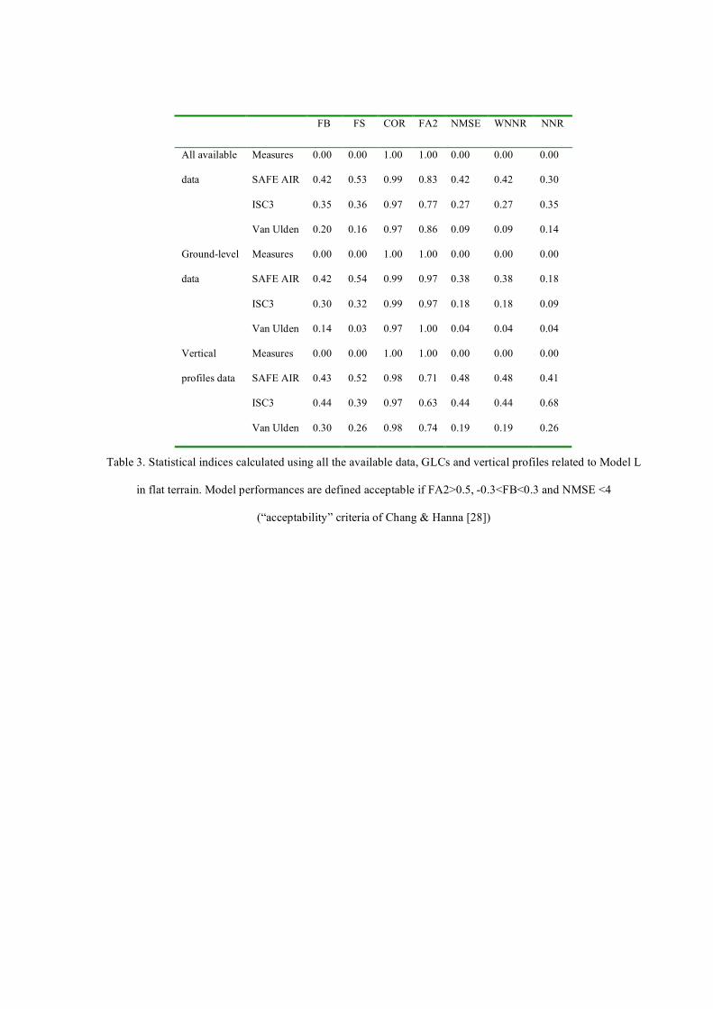
Moreover, the “acceptability” criterion of Chang and Hanna [28] has been used, where models

performances are defined acceptable if FA2>0.5, -0.3<FB<0.3 and NMSE <4.

Reference data used in the validation exercise are the concentration profiles measured during the

experiments with Model H and flat terrain, appropriately converted to the full scale values.

3. RESULTS

3.1 Experiments with the Model H

Hot-wire anemometry measures

Vertical mean wind flow and turbulence intensity profiles (fig. 4) show a considerable reduction in

terms of wind velocity (speed at a height of 5 cm changes from 2 m/s for flat terrain to 0.4 m/s in

presence of the landfill) and a substantial increase of turbulence intensity compared to the reference

profile. These flow modifications induced by the landfill relief are remarkable in the BL lower levels

and their influence decreases along z-axis and with distance along x-axis; disturbance effects are still

significant at a distance of x=257 cm.

Comparisons of measures carried out with the two models (fig. 5 and 6) put in evidence that an

increase of model height causes an intensification of the flow modifications, characterised by a greater

decrease of the wind velocity and an increase of the turbulent phenomena downwind of the model (fig.

5). In the presence of Model L, the disturbance effects decrease more quickly with the height and with

the distance compared to Model H; the modification effects disappear at x=157 cm (fig. 6).

Tracer concentration measurements

The concentration results are reported in the non-dimensional form of equation (1). The mean

concentration profile along the centreline is reported in figure 7 (top-left). The highest concentrations

can be observed close to the landfill relief; the gradient has higher values next to the emission source

and decreases with distance down to near zero at the end of the working section. Transverse

concentration profiles (fig. 7, top-right) show a symmetric behaviour and a progressive plume spread

in the y-direction when the distance from the model increases (fig. 8, right). Vertical profiles (fig. 7,

bottom-left) show a characteristic rising and expanding bent-over plume. Wind tunnel measurements

also allowed a ground-level concentration map to be constructed (fig. 7 bottom-right).

Different dispersion parameters have been calculated using experimental measures, i.e. mean height of

the plume, <z>, and vertical and lateral spread (sigmaz and sigmay), in order to analyze the plume

behaviour downwind of the source.

( ) ( )!!""

>=<00

dzzCdzzzCz ( ) ( ) ( )!!""

><#=00

22 dzzCdzzCzzsigmaz

( ) ( )!!""

=00

22 dyyCdyyCysigmay

The mean height of the plume (fig. 8, left) is lower than the emission height (equal to 13 cm) along the

whole working section of the BWLT. This result demonstrates how turbulent flow and streamline

deflection downwind of the landfill deflect downwards the tracer, causing an increase on the ground

level concentrations (GLCs). Besides, it is possible to observe a constant growth of the plume height,

due to the presence of reflection effects of the ground. The plotted variation of sigmaz and sigmay (fig.

8, left) versus distance shows the vertical and lateral spreads of the plume, showing a decreasing

spread rate with increasing distance.

Comparisons of measures carried out with the two models at different flow speeds (fig. 9), show how

dispersion behaviour, in terms of non-dimensional concentration, is dependent to geometric shape of

the source, but independent to wind speed. For the Model H case we can observe lower concentrations

near the ground and higher concentrations at higher levels. This phenomenon is justified by the higher

emission height and by a much greater turbulence intensity that characterised the Model H

configuration; as a matter of fact, these elements cause a large spread and consequently a decrease of

the tracer concentrations. Wind speed invariance allowed us to check the non-dimensional

concentration parameters used during the experiments.

3.2 Experiments with Model L in complex terrain

Hot-wire anemometry measures

The presence of the hill downwind of the landfill causes a flow deflection characterised by an increase

of the wind velocity above the hill and a small modification of wind flow downwind of the hill (fig.

11,); disturbance effects (increase of turbulence intensity and decrease of wind velocity), as a matter of

fact, affect only the lower part of the BL and vanish at a distance of about 60 cm from the hill, at

x=257 cm (fig. 12). Upwind from the hill (fig. 10), on the contrary, wind flow seems unchanged,

vertical mean wind flow and intensity turbulence profiles results substantially the same in both the

cases (with and without the hill).

Tracer concentration measurements

Longitudinal, transversal and vertical profiles in this second configuration, following the same

methodology of the previous case, are reported in figure 13; a GLC map (fig. 13, bottom-right) and

estimates of some dispersion parameters (fig. 14) were also produced.

Comparing the data (fig. 15) from the flat and gentle terrain configurations, it can be noted how,

upwind of the hill, the dispersion behaviour remains substantially unchanged (non-dimensional

concentration and flow characteristics keep similar values); downwind from the hill a small decrease

of GLC and an increase of tracer concentration at elevated heights can be observed; this fact is due to

tracer deflection and to induced turbulence related to the presence of the hill. When the distance from

hill increases, disturbance effects tend to disappear quickly. Thus, it can be stated that changes induced

by the hill (gentle terrain) does not modify too much pollutant levels and the dispersion behaviour.

3.3 PIV experiments

PIV measurements performed downwind from the landfill allow to obtain velocity contour, vector and

vorticity maps related to several horizontal and vertical sections.

Horizontal visualizations (fig. 16) show that the direction of the flow is quite uniform, while the wind

speed increases with the distance from the landfill; x-y plane measurements do not show the presence

of vortices. This is also confirmed by vorticity maps, which show (fig. 17) a small variability.

However, the landfill relief does not seem to sensibly affect the flow behaviour on parallel planes to

the ground.

Vertical sections (fig. 18 and 20) show a regularity of the flow direction as well. The measurements ,

however, did highlight the downwards flow deflection (fig. 18) and higher vorticity (fig. 19).

However, this effect vanished at x=70 cm from the landfill centre, where the parallel flow is

established again (fig. 20) and the vorticity is less variable (fig. 21).

3.4 Model validation exercise

A sensitivity analysis on the three mathematical models was carried out considering different

parameters, such as the downwash effect, the dispersion coefficients σz and σy, the number of point

sources (for the simulation of the area source) and flow speed (table 1). This study allowed us to

establish calibration conditions and to define the most important elements in model performances.

Statistical analysis and graphical comparisons show, as reported in table 1, that all codes are very

sensible to the downwash effect induced by the landfill relief; as a matter of fact, the models tend to

underestimate GLCs if no “downwash effect” correction is applied. The number of circular sources

and the flow speed are less important for model performance, while the choice of dispersion

coefficients is rather significant, particularly for Gaussian models.

The best configurations for the codes resulting from the sensitivity analysis are the following:

- SAFE AIR: emission area simulated using 49 circular sources; emission height He = 0; Briggs

“open country” σ-functions.

- ISC3: area source algorithm; He = 0; rural σ-functions.

- Van Ulden: emission area simulated using 49 circular sources; He = 5.8 m; Pasquill-Gifford-

Turner σ-functions.

Statistical analysis (tab. 2) and graphical comparisons (fig. 22) of the calibrated models show how all

the models have much greater difficulties in the reproduction of vertical profiles, while GLC

predictions are definitely better. The acceptability criteria of Chang and Hanna [28] is verified only for

GLC data. The best model seems to be the Van Ulden code, although SAFE_AIR also performs

reasonably well; the worst performing model in the present case, according to this analysis, is ISC3.

For a better understanding of models capabilities, a comparison with the experiments on model L has

been performed. Statistical analysis and graphical comparisons related to this configuration are

reported respectively in table 3 and figure 23.

Van Ulden model is the best also in this case. As a matter of fact, by adjusting the emission height in

the algorithm it was possible to verify the Chang and Hanna criteria [28].

Compared to validation exercises for simpler cases (such as standard single stack point sources and

flat terrain) [29] [30], this study shows that the models predictions are less satisfactory; in the point

source cases, mathematical simulation results verify Chang and Hanna criteria both for the GLC data

and the vertical profiles. This conclusion was expected because the applied models were originally

built to simulate point sources at elevated heights.

4. CONCLUSIONS

Wind tunnel experiments have been carried out on small scale physical models of landfills. The large

experimental data-set obtained in this study are very useful for the following purposes:

1. Characterization and understanding of pollutant dispersion downwind from an elevated area

source.

2. Development and verification of physical small-scale models representing MWL.

3. Calibration and performance evaluation of mathematical models.

In order to show the potentiality and the usefulness of the data produced they have been further

analysed and applied in a validation exercise involving some mathematical models.

The experiments highlighted an increase of pollutant GLC immediately downwind from the landfill

due to induced turbulence and mean flow deflection. This phenomenon is similar to the “downwash

effect” in industrial buildings and turns out to be predominant for the dispersion process; its

identification was obtained by longitudinal and vertical concentration profiles with different set-ups

and by an evaluation of mean plume height. Besides, the presence of the downwash effect is

confirmed by mathematical model simulations, that show how not considering the downwash effect

causes an underestimation of GLC. Tests with a different landfill height and in complex terrain were

also very useful. The former showed an important dependence of the dispersion phenomena from the

landfill height, while the latter highlighted how gentle orographic conditions downwind of the landfill

do not affect significantly the dispersion behaviour.

To check the validity of the experimental set-up, a verification of the non-dimensional concentration

parameter used during the experiments was carried out. Wind speed independence was demonstrated

for this purpose.

Validation exercises were useful for model calibration, improving code reliability, as well as

evaluating performance. As far as this study is concerned, simulations using the Van Ulden model are

the most encouraging. Results obtained from this model are acceptable according to the Chang &

Hanna criterion [28].

The obtained data-set can be further extended and improved in future experiments. For example,

future experiments can include different wind directions and hills with different shape, as well as more

complex terrains downwind form the landfill relief.

5. REFERENCES

[1] El-Fadel, M., Findikakis, A.N. & Leckie, J.O. (1997). Environmental impacts of solid waste

landfilling. Journal of Environmental Management, 50, 1-25

[2] Sarkar, U. & Hobbs, S.E. (2003). Landfill odour: assessment of emissions by the flux footprint

method. Environmental Modelling and Software, 18, 155-163

[3] Sarkar, U., Hobbs, S.E. & Longhurst, P. (2003). Dispersion of odour: a case study with a municipal

solid waste landfill site in North London, United Kingdom. Journal of Environmental Management,

68, 153-160

[4] Borrego, C., Schatzmann, M. & Galmarini, S. (2003). Quality assurance of air quality models. (In

Moussiopoulos, N. (Ed.), SATURN – Studying atmospheric pollution in urban areas – EUROTRAC2

subproject final report (pp. 155-183). Heidelberg: Springer Verlag)

[5] Schatzmann, M., Rafailidis, S. & Pavageau, M. (1997). Some remarks on the validation of small-

scale dispersion models with field and laboratory data. Journal of Wind Engineering and Industrial

Aerodynamics, 67-68, 885-893

[6] Schatzmann, M. & Leitl, B. (2002). Validation and application of obstacle-resolving urban

dispersion models. Atmospheric Environment 36, 4811-4821

[7] Van Aalst, R., Edwards, L., Pulles, T., De Saeger, E., Tombrou, M. & Tønnesen, D. (1998).

Guidance report on preliminary assessment under EC air quality directives. Technical Report no. 11

(European Environment Agency)

[8] Hanna, S.R. (1988). Air quality model evaluation and uncertainty. JAPCA – The International

Journal of the Air Pollution Control Association, 38, 406-412

[9] Hanna, S.R. (1993). Uncertainties in air-quality model predictions. Boundary-Layer Meteorology,

62, 3-20

[10] Weil, J.C, Sykes, R.I. & Venkatram, A. (1992). Evaluating air-quality models – Review and

outlook. Journal of Applied Meteorology, 31, 1121-1145

[11] Hanna, S.R. (1989). Confidence limits for air quality model evaluations as estimated by bootstrap

and jackknife resampling methods. Atmospheric Environment, 23, 1385-1398

[12] Olesen, H.R. (2005). User’s guide to the Model Validation Kit. Initiative on Harmonisation

within Atmospheric Dispersion Modelling for Regulatory Purposes, from http://www.harmo.org/kit

[13] ASTM (2000). Standard guide for statistical evaluation of atmospheric model performance.

American Society of Testing and Materials, D 6589-00

[14] Carpentieri, M. (2006). Modelling air quality in urban areas. PhD thesis, University of Florence

[15] Cavallaro, M., Canepa, E. & Ratto, C.F. (2003, September). A validation exercise of the P6

dispersion model using wind tunnel data about area source. (Paper presented at the PHYSMOD2003

Workshop, Prato, Italy)

[16] Carpentieri, M., Corti, A. & Zipoli, L. (2004). Wind tunnel experiment of tracer dispersion

downwind from a small-scale physical model of a landfill. Environmental Modelling and Software,

19, 881-885

[17] Canepa, E. & Builtjes, P.J.H. (2001). Methodology of model testing and application to dispersion

simulation above complex terrain. International Journal of Environment and Pollution, 16, 101-115

[18] Augusti, G., Borri, C., Giordano, S., Spinelli, P. & Niemann, H. (1990). Il progetto della galleria

del vento a strato limite sviluppato dall’Università di Firenze (Paper presented at the 1st Convegno

nazionale di Ingegneria del Vento, Firenze, Italy)

[19] Zipoli, L. (2002). Misure anemometriche e diffusionali in galleria del vento applicate al caso di

emissione di tracciante inquinante da discariche di R.S.U. Dissertation, University of Florence

[20] Nicolas, J., Craffe, F. & Romain, A.C. (2006). Estimation of odor emission rate from landfill

areas using the sniffing team method. Waste Management, 26, 1259-1269

[21] Robins, A.G. (1977). Wind tunnel modelling of plume dispersal. CEGB Report R/M/R247,

Central Electricity Generating Board, Research Division, Marchwood Engineering Laboratories

[22] Obasaju, E.D. & Robins, A.G. (1998). Simulation of pollutant dispersion using small scale

models - an assessment of scaling options. Environmental Monitoring and Assessment, 52, 239-254

[23] Scaperdas, A. (2000). Modelling air flow and pollutant dispersion at urban canyon intersections.

PhD Thesis, Imperial College of Science and Technology, University of London

[24] U.S. EPA (1992). Comparison of a revised area source algorithm for the industrial source

complex short term model and wind tunnel data. EPA-454/R-92-014.

[25] Van Ulden, A.P. (1978). Simple estimates for vertical diffusion from sources near the ground.

Atmospheric Environment, 12, 2125-2129

[26] Hanna, S.R., Strimaitis, D.G. & Chang, J.C. (1991). Hazard response modelling uncertainty (a

quantitative method): User’s guide for software for evaluation of hazardous gas dispersion models.

Final Report, vol. I (Westford: Sigma Research Corp.)

[27] Poli, A.A. & Cirillo, M.C. (1993). On the use of the normalized mean square error in evaluating

dispersion model performance. Atmospheric Environment, 15, 2427-2434

[28] Chang, J.C. & Hanna, S.R. (2004). Air quality model performance evaluation. Meteorology and

Atmospheric Physics, 87, 167-196

[29] Manfrida, G., Corti, A. & Contini, D. (1999, October). Comparison between different dispersion

models with wind tunnel small scale measurements. (Paper presented at the 6th International

Conference on Harmonization within Atmospheric Dispersion Modelling for Regulatory Purposes,

Rouen, France)

[30] Corti, A., Zanobini, M. & Canepa, E. (2002). Use of wind tunnel measurements for mathematical

comparison and validation. (In Sportisse, B. (Ed.), Air Pollution Modelling and Simulation (pp. 341-

354). Heidelberg: Springer-Verlag)

TABLES:

Sensitivity analysis Sensitivity level Calibration conditions

N° of circle sources low 49 sources

Initial-σ low (0;0;0.369Ds)

Downwash effect high He = 0

Dispersion coeff. σ medium Briggs open country

SAFE AIR

Wind speed low v = 2 m/s at 10 m

Downwash effect high Area source algorithm (He=0) ISC3

Wind speed null -

n° of circe source low 49 sources

Dispersion coeff. σy low P-G-T

Downwash effect high He = 5.8 m

VAN ULDEN

Wind speed null -

Table 1. Sensitivity analysis results

FB FS COR FA2 NMSE WNNR NNR

Measures 0.00 0.00 1.00 1.00 0.00 0.00 0.00

SAFE AIR 0.11 0.10 0.92 0.76 0.17 0.19 0.28

ISC3 -0.17 -0.29 0.89 0.71 0.34 0.44 0.54

All available

data

Van Ulden 0.09 0.14 0.92 0.74 0.18 0.20 0.22

Measures 0.00 0.00 1.00 1.00 0.00 0.00 0.00

SAFE AIR 0.00 0.07 0.97 0.99 0.03 0.03 0.03

ISC3 -0.32 -0.33 0.98 0.97 0.21 0.20 0.13

Ground-level

data

Van Ulden -0.01 0.12 0.96 0.97 0.07 0.08 0.05

Measures 0.00 0.00 1.00 1.00 0.00 0.00 0.00

SAFE AIR 0.53 0.17 0.79 0.38 0.93 0.95 1.08

ISC3 0.52 -0.16 0.69 0.30 1.30 1.66 2.21

Vertical

profiles data

Van Ulden 0.46 0.18 0.82 0.37 0.74 0.75 0.70

Table 2. Statistical indices calculated using all the available data, GLCs and vertical profiles related to Model H

in flat terrain. Model performances are defined acceptable if FA2>0.5, -0.3<FB<0.3 and NMSE <4

(“acceptability” criteria of Chang & Hanna [28])

FB FS COR FA2 NMSE WNNR NNR

Measures 0.00 0.00 1.00 1.00 0.00 0.00 0.00

SAFE AIR 0.42 0.53 0.99 0.83 0.42 0.42 0.30

ISC3 0.35 0.36 0.97 0.77 0.27 0.27 0.35

All available

data

Van Ulden 0.20 0.16 0.97 0.86 0.09 0.09 0.14

Measures 0.00 0.00 1.00 1.00 0.00 0.00 0.00

SAFE AIR 0.42 0.54 0.99 0.97 0.38 0.38 0.18

ISC3 0.30 0.32 0.99 0.97 0.18 0.18 0.09

Ground-level

data

Van Ulden 0.14 0.03 0.97 1.00 0.04 0.04 0.04

Measures 0.00 0.00 1.00 1.00 0.00 0.00 0.00

SAFE AIR 0.43 0.52 0.98 0.71 0.48 0.48 0.41

ISC3 0.44 0.39 0.97 0.63 0.44 0.44 0.68

Vertical

profiles data

Van Ulden 0.30 0.26 0.98 0.74 0.19 0.19 0.26

Table 3. Statistical indices calculated using all the available data, GLCs and vertical profiles related to Model L

in flat terrain. Model performances are defined acceptable if FA2>0.5, -0.3<FB<0.3 and NMSE <4

(“acceptability” criteria of Chang & Hanna [28])

FIGURES:

Figure 1. Vortex generators (Irwin and Counihan spires) located at the beginning of the flow development zone

Figure 2. Mean flow vertical profiles (left) and turbulence intensity profiles Ix(right) without landfill model along

the centreline

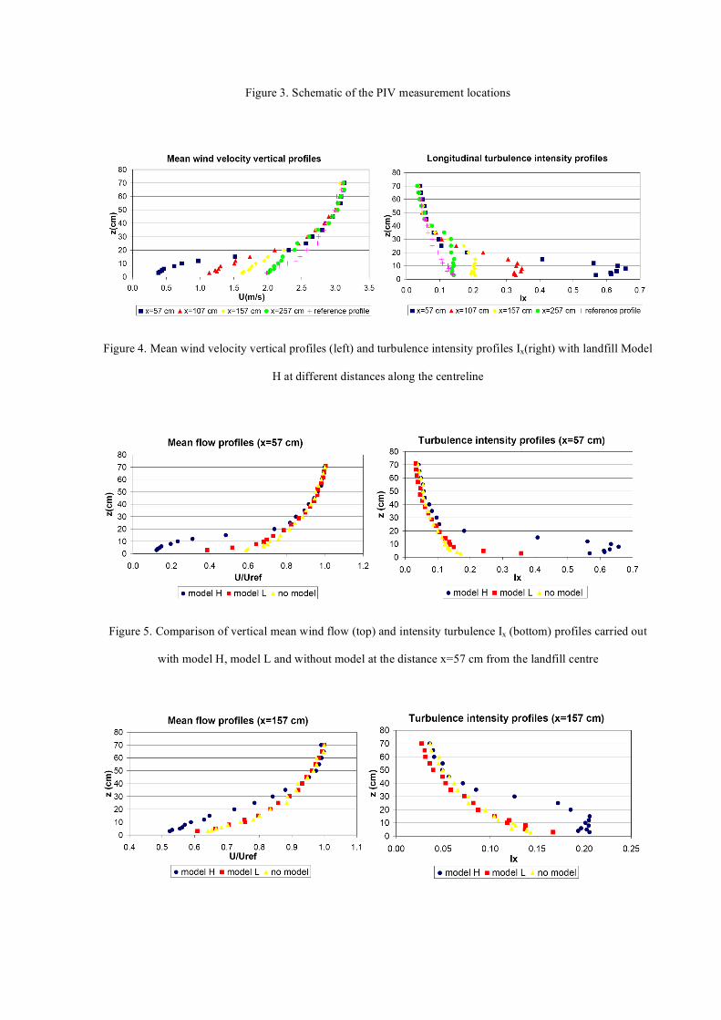
Figure 3. Schematic of the PIV measurement locations

Figure 4. Mean wind velocity vertical profiles (left) and turbulence intensity profiles Ix(right) with landfill Model

H at different distances along the centreline

Figure 5. Comparison of vertical mean wind flow (top) and intensity turbulence Ix (bottom) profiles carried out

with model H, model L and without model at the distance x=57 cm from the landfill centre

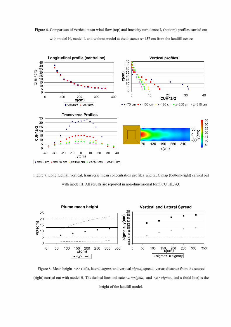
Figure 6. Comparison of vertical mean wind flow (top) and intensity turbulence Ix (bottom) profiles carried out

with model H, model L and without model at the distance x=157 cm from the landfill centre

Figure 7. Longitudinal, vertical, transverse mean concentration profiles and GLC map (bottom-right) carried out

with model H. All results are reported in non-dimensional form CUrefHref/Q.

Figure 8. Mean height <z> (left), lateral sigmay and vertical sigmaz spread versus distance from the source

(right) carried out with model H. The dashed lines indicate <z>+sigmaz and <z>-sigmaz and h (bold line) is the

height of the landfill model.

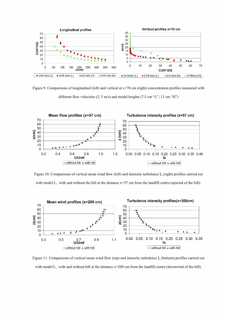
Figure 9. Comparisons of longitudinal (left) and vertical at x=70 cm (right) concentration profiles measured with

different flow velocities (2, 5 m/s) and model heights (7.5 cm “L”; 13 cm “H”)

Figure 10. Comparisons of vertical mean wind flow (left) and intensity turbulence Ix (right) profiles carried out

with model L, with and without the hill at the distance x=57 cm from the landfill centre (upwind of the hill).

Figure 11. Comparisons of vertical mean wind flow (top) and intensity turbulence Ix (bottom) profiles carried out

with model L, with and without hill at the distance x=200 cm from the landfill centre (downwind of the hill).

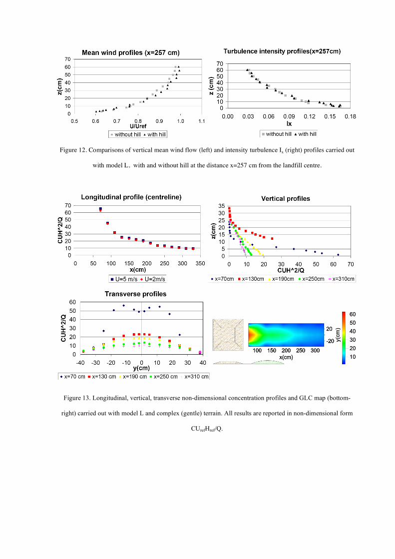
Figure 12. Comparisons of vertical mean wind flow (left) and intensity turbulence Ix (right) profiles carried out

with model L, with and without hill at the distance x=257 cm from the landfill centre.

Figure 13. Longitudinal, vertical, transverse non-dimensional concentration profiles and GLC map (bottom-

right) carried out with model L and complex (gentle) terrain. All results are reported in non-dimensional form

CUrefHref/Q.

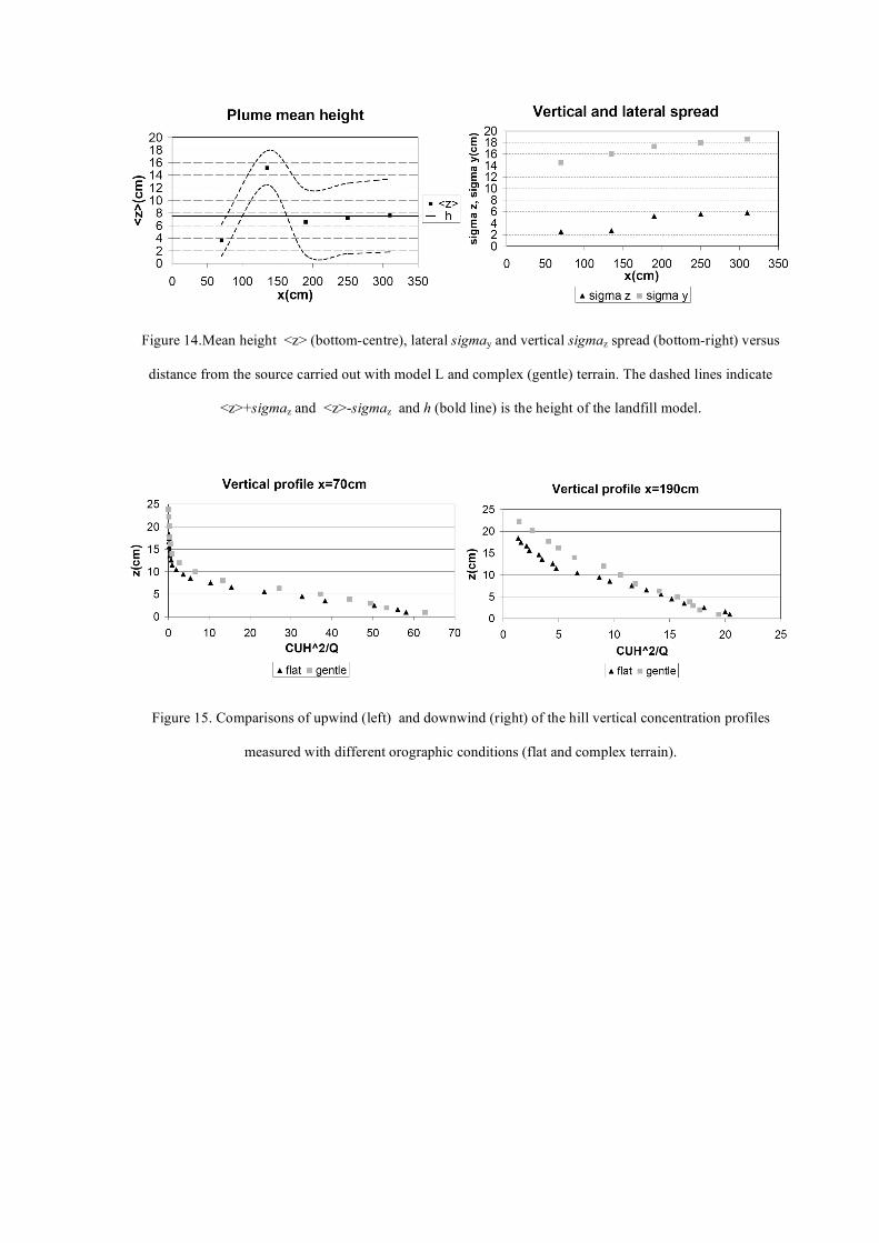
Figure 14.Mean height <z> (bottom-centre), lateral sigmay and vertical sigmaz spread (bottom-right) versus

distance from the source carried out with model L and complex (gentle) terrain. The dashed lines indicate

<z>+sigmaz and <z>-sigmaz and h (bold line) is the height of the landfill model.

Figure 15. Comparisons of upwind (left) and downwind (right) of the hill vertical concentration profiles

measured with different orographic conditions (flat and complex terrain).

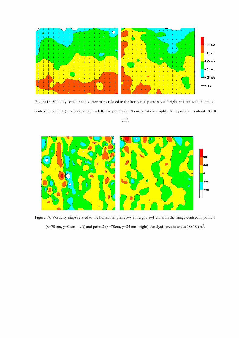
Figure 16. Velocity contour and vector maps related to the horizontal plane x-y at height z=1 cm with the image

centred in point 1 (x=70 cm, y=0 cm - left) and point 2 (x=70cm, y=24 cm - right). Analysis area is about 18x18

cm2.

Figure 17. Vorticity maps related to the horizontal plane x-y at height z=1 cm with the image centred in point 1

(x=70 cm, y=0 cm - left) and point 2 (x=70cm, y=24 cm - right). Analysis area is about 18x18 cm2.

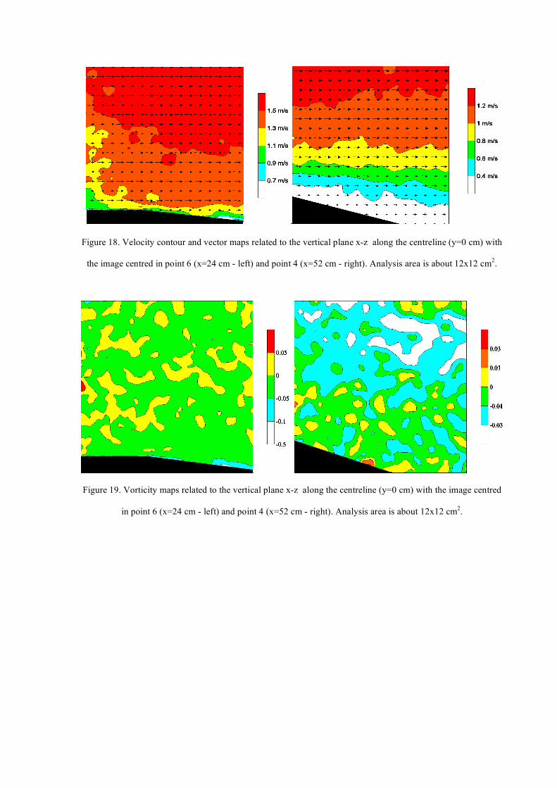
Figure 18. Velocity contour and vector maps related to the vertical plane x-z along the centreline (y=0 cm) with

the image centred in point 6 (x=24 cm - left) and point 4 (x=52 cm - right). Analysis area is about 12x12 cm2.

Figure 19. Vorticity maps related to the vertical plane x-z along the centreline (y=0 cm) with the image centred

in point 6 (x=24 cm - left) and point 4 (x=52 cm - right). Analysis area is about 12x12 cm2.

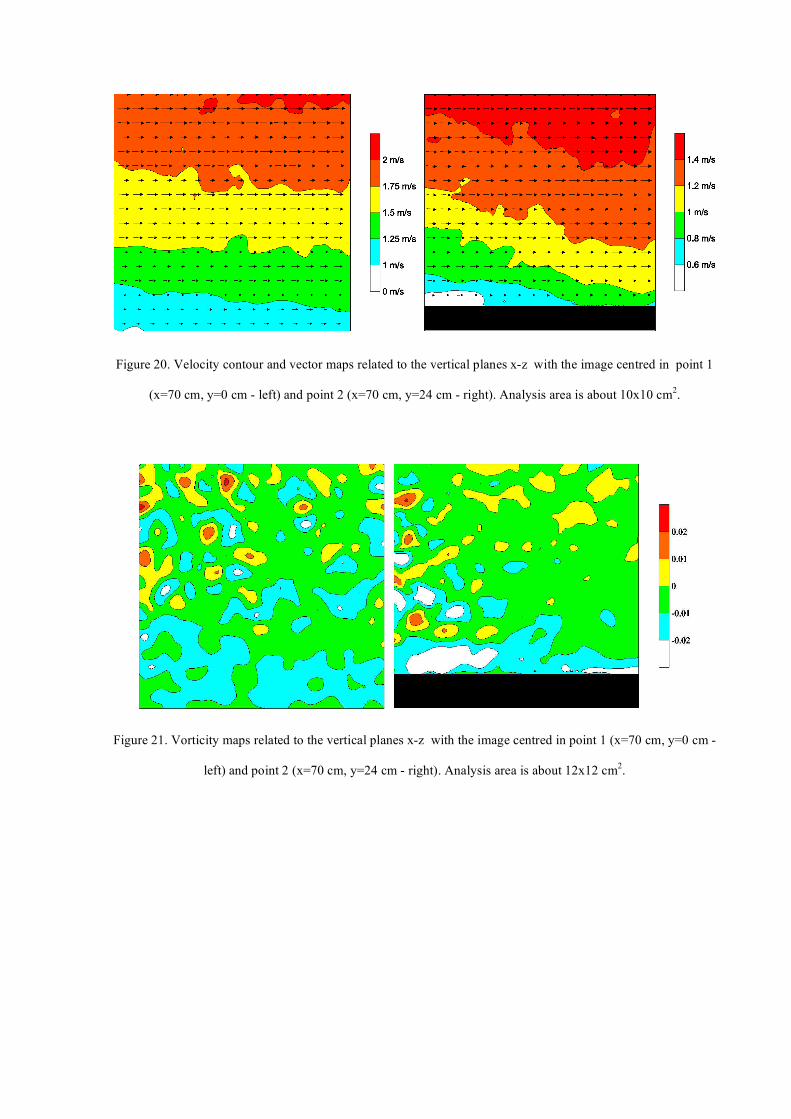
Figure 20. Velocity contour and vector maps related to the vertical planes x-z with the image centred in point 1

(x=70 cm, y=0 cm - left) and point 2 (x=70 cm, y=24 cm - right). Analysis area is about 10x10 cm2.

Figure 21. Vorticity maps related to the vertical planes x-z with the image centred in point 1 (x=70 cm, y=0 cm -

left) and point 2 (x=70 cm, y=24 cm - right). Analysis area is about 12x12 cm2.

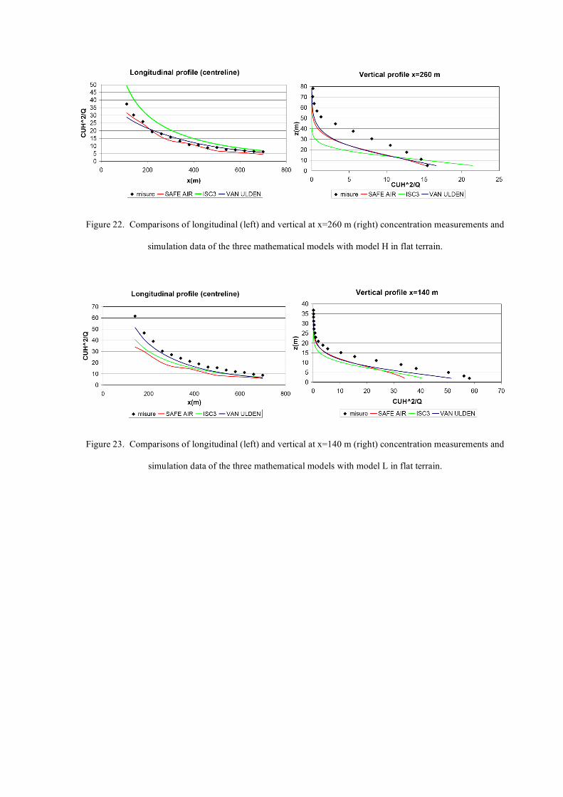
Figure 22. Comparisons of longitudinal (left) and vertical at x=260 m (right) concentration measurements and

simulation data of the three mathematical models with model H in flat terrain.

Figure 23. Comparisons of longitudinal (left) and vertical at x=140 m (right) concentration measurements and

simulation data of the three mathematical models with model L in flat terrain.