Embed Size (px)
Citation preview
Study of the hydrodynamics and morphodynamics of the
Óbidos lagoon, Portugal
Diogo Silva Mendes
Dissertation to obtain the Master of Science Degree in
Civil Engineering
(Hydraulics and Water Resources)
Supervisors: Dr. André Bustorff Fortunato and Prof. António Alberto Pires Silva
Examination Committee
Chairperson: Prof. António Alexandre Trigo Teixeira
Supervisor: Dr. André Bustorff Fortunato
Member of the Committee: Dr. Xavier Pierre Jean Bertin
Member of the Committee: Dr. Anabela Pacheco de Oliveira
March 2015

Study of the hydrodynamics and morphodynamics of the
Óbidos lagoon, Portugal
Estudo sobre a hidrodinâmica e a morfodinâmica da lagoa de
Óbidos, Portugal
Diogo Silva Mendes
Dissertation to obtain the Master of Science Degree in
Civil Engineering
(Hydraulics and Water Resources)
Supervisors: Dr. André Bustorff Fortunato and Prof. António Alberto Pires Silva
Examination Committee
Chairperson: Prof. António Alexandre Trigo Teixeira
Supervisor: Dr. André Bustorff Fortunato
Member of the Committee: Dr. Xavier Pierre Jean Bertin
Member of the Committee: Dr. Anabela Pacheco de Oliveira
March 2015


RESUMO
Na lagoa de Óbidos, as ondas e as correntes de maré induzem rápidas alterações morfológicas levando ao
fecho da sua embocadura. As dragagens são frequentes tendo o objetivo de manter a laguna aberta e
proteger as construções marginais. No entanto, o efeito das dragagens no comportamento da embocadura
é um tema pouco estudado, especialmente o impacto que poderá ter a adição de canais transversais aos
tradicionais canais dragados.
No interior desta laguna as ondas induzem alterações significativas nas condições hidrodinâmicas.
Através da aplicação de um modelo acoplado constituído por um modelo hidrodinâmico e um modelo de
agitação marítima concluiu-se que as elevações da superfície livre dentro da lagoa aumentaram para uma
direcção média da onda perpendicular à linha de costa. Foi também investigado o impacto que a
interacção completa entre ondas e correntes tem na dinâmica sedimentar da lagoa de Óbidos, concluindo-
se que o transporte de sedimentos para o interior aumenta em 30% durante a enchente se esta interacção
for tida em conta no modelo numérico.
Os três planos de dragagens foram avaliados através da implementação de um modelo morfodinâmico. Os
novos planos de dragagens aumentaram o prisma de maré e reduziram as diferenças de duração entre a
vazante e a enchente devido aos canais principais norte e sul. Os canais transversais aumentaram o
assoreamento no canal principal sul e promoveram a estabilidade do canal principal norte. No entanto,
devido às baixas profundidades e a uma agitação marítima muito energética, as soluções de dragagens são
incapazes estabilizar permanentemente a lagoa de Óbidos.
PALAVRAS-CHAVE: Modelação morfodinâmica, Dragagens, Processos induzidos pelas ondas,
Embocaduras de maré, Canais transversais, Profundidade de equilíbrio de dragagem

ABSTRACT
In the Óbidos lagoon, waves and tidal currents induce rapid morphological changes driving its inlet to
closure. Dredging solutions are frequent in order to reposition the inlet in a central location and to deepen
the main channels, therefore, preventing the inlet’s closure. However, less is known about the effect of
dredging solutions on the inlet’s behaviour, especially the addition of transverse channels to the main
dredged channels in dredging solutions.
Waves induce important changes in the hydrodynamics inside the Óbidos lagoon. The effect of mean
wave direction on the water levels inside the lagoon was studied using a fully-coupled hydrodynamic and
wave model. The water levels increased with the mean wave direction perpendicular to the coastline. The
impact of the full interaction between waves and currents on the sediment dynamics in the Óbidos lagoon
was also investigated. This study concludes that the sediment transport during the flood towards the
lagoon increases 30% if the previous interaction was considered by the numerical model.
The three dredging plans were assessed by implementing and exploiting a morphodynamic model. The
new dredging plans increased the tidal prism and reduced the differences between the ebb and flood
durations mainly due to the southern and northern main channels. The transverse channels increased the
accretion of the southern main channel and promoted the stability of the northern main channel. However,
due to the shallow depths and the very energetic wave regime, dredging solutions are unable to
permanently stabilize the Óbidos lagoon.
KEYWORDS: Morphodynamic model, Dredging, Wave-induced processes, Tidal inlets, Transverse
channels, Dredging equilibrium depth

ACKNOWLEDGEMENTS
Firstly, I would like to acknowledge my supervisors – Dr. André Fortunato and Professor António Pires
Silva. Thank you André for all the knowledge transmitted during this period and also for the constructive
criticism that strongly contributed for the final result of this dissertation. Thank you Professor for your
fully availability to clarify any doubt or question, and they were many. Thank you both for all your rigor
and exigency deposited in this dissertation.
Gratitude is expressed to LNEC for making available the realization of this dissertation, providing me an
office, where I stayed the last year. I would like to leave a special acknowledge to Kai Li and to Dr.
Alberto Azevedo, the first for all his tireless help in Linux, and the second for providing me tools to make
brilliant figures. Thanks also to Dr. Guillaume Dodet and to Thomas Guerin for their advices on the
morphodynamic model, and to Alphonse Nahon to provide the value of the gross annual littoral drift for
the Óbidos lagoon.
To the developers of SELFE, WWM-II and SED2D for making their source codes available. This work
makes use of results produced with the support of the Portuguese National Grid Initiative, more
information in https://wiki.ncg.ingrid.pt.
To Anabela Montenegro, Zé Rua and André Morais for their review and improvements on this document,
and also to Diogo Simões for his help in developing some excellent figures.
To all my friends, from ISEL in the bachelor to the IST in the master, and also, all the friends outside
school, for your support.
To my family for everything.
In the end, I want to briefly acknowledge Cláudia for all her patience during this period and for the
weekend that she provides me in the Óbidos lagoon, two months after the beginning of this dissertation.
For sure that if I don’t acknowledge her briefly, all the pages in this dissertation will not be enough to
express my gratitude to her.

LIST OF CONTENTS
LIST OF FIGURES .................................................................................................................................... I
LIST OF TABLES ..................................................................................................................................... V
LIST OF SYMBOLS .............................................................................................................................. VII
LIST OF ACRONYMS ........................................................................................................................... IX
1. Introduction ....................................................................................................................................... 1
1.1. The importance of tidal inlets: Óbidos lagoon inlet..................................................................... 1
1.2. Objectives and general methodology........................................................................................... 2
1.3. Outline of the dissertation............................................................................................................ 2
2. Tidal inlets brief background review and the case study: the Óbidos lagoon .............................. 5
2.1. Tidal inlets ................................................................................................................................... 5
2.1.1. Inlet morphological components ............................................................................................ 5
2.1.2. Inlet classification and stability .............................................................................................. 6
2.1.3. Morphodynamic models for tidal inlets – some examples ..................................................... 9
2.2. Study site - the Óbidos lagoon ................................................................................................... 12
2.2.1. Geomorphological and hydrodynamic settings of the Óbidos lagoon .................................. 12
2.2.2. Long and short time scales of the morphosedimentary evolution ......................................... 14
2.2.3. Coastal management and human interventions in the last decades ....................................... 15
3. The influence of external forcing on the Óbidos lagoon hydrodynamics .................................... 19
3.1. Brief review on the effect of waves in the hydrodynamics of two Portuguese coastal
lagoons....................................................................................................................................... 19
3.2. Methodology - a two-way coupling between SELFE and WWM-II ......................................... 19
3.2.1. General scheme..................................................................................................................... 19
3.2.2. The wave model – WWM-II ................................................................................................. 20
3.2.3. The hydrodynamic model - SELFE ...................................................................................... 21
3.2.4. Boundary conditions and numerical grid .............................................................................. 21
3.2.5. Wave climate verification period and statistical error measures .......................................... 23
3.2.6. Water levels verification period and statistical error measures ............................................ 24
3.2.7. Idealized scenarios to study the influence of waves on the Óbidos lagoon .......................... 24
3.3. Analysis and discussion of the results ....................................................................................... 25
3.3.1. Comparisons between ADCP measurements and WWM-II simulations.............................. 25

3.3.2. Comparisons between tidal gauge measurements and coupled SELFE and WWM-II
simulations ........................................................................................................................... 27
3.3.3. Sensitivity analysis of the wave parameters on the Óbidos lagoon hydrodynamics ............. 27
3.3.4. The wave blocking phenomenon .......................................................................................... 32
4. Assessment of three dredging plans for the Óbidos lagoon .......................................................... 35
4.1. Review on seasonal closure, tidal distortions and dredging solutions in wave-dominated
inlets .......................................................................................................................................... 35
4.2. The morphodynamic model and the implemented methodology............................................... 37
4.2.1. Morphodynamic model general outline ................................................................................ 37
4.2.2. The sediment transport and bottom evolution model – SED2D ........................................... 38
4.2.3. Sediment model verification period and statistical error measures ...................................... 39
4.2.4. Boundary conditions of the sediment model ........................................................................ 40
4.2.5. The simulated dredging plans under study ........................................................................... 40
4.3. The verification of the bathymetry simulated until November 2001 ......................................... 41
4.3.1. The qualitative and quantitative morphodynamic model simulation .................................... 41
4.3.2. The evolution of the M2 harmonic constituent amplitude ..................................................... 43
4.4. The impact of dredging plans on the inlet’s behaviour .............................................................. 44
4.4.1. Qualitative evolution of the inlet .......................................................................................... 44
4.4.2. Evolution of the tidal prism .................................................................................................. 45
4.4.3. Differences in ebb-flood durations ....................................................................................... 46
4.4.4. The Óbidos lagoon ability to flush out sediments ................................................................ 48
4.4.5. The application of empirical stability relationships to the Óbidos lagoon inlet .................... 50
4.5. Summary ................................................................................................................................... 52
5. Conclusions and future research .................................................................................................... 55
Bibliographic references .......................................................................................................................... 57
APPENDIX A - Governing equations of the numerical models ............................................................. i
APPENDIX B - Velocity fields during the ebb and the changed parameters in SELFE .................... v
APPENDIX C - Modified boundary conditions in SED2D .................................................................. vii
APPENDIX D - Five-month evolution of the dredging plan proposed by Fortunato
and Oliveira (2007a) (DP2) ........................................................................................... ix
APPENDIX E - Five-month evolution of the dredging plan proposed by Fortunato
and Oliveira (2007a) with only one transverse channel (DP3) .................................. xi

APPENDIX F - Comparison between the modelled and measured on the wave gauge
and WW3 wave parameters for each WW3 station (numbering from
right to left and top to bottom) ...................................................................................xiii
APPENDIX G – Asymptotically evolution of the bottom depth calculated for the
three measured bathymetries available (July 2001, November 2001
and April 2002) at the flood delta ............................................................................... xv

I
LIST OF FIGURES
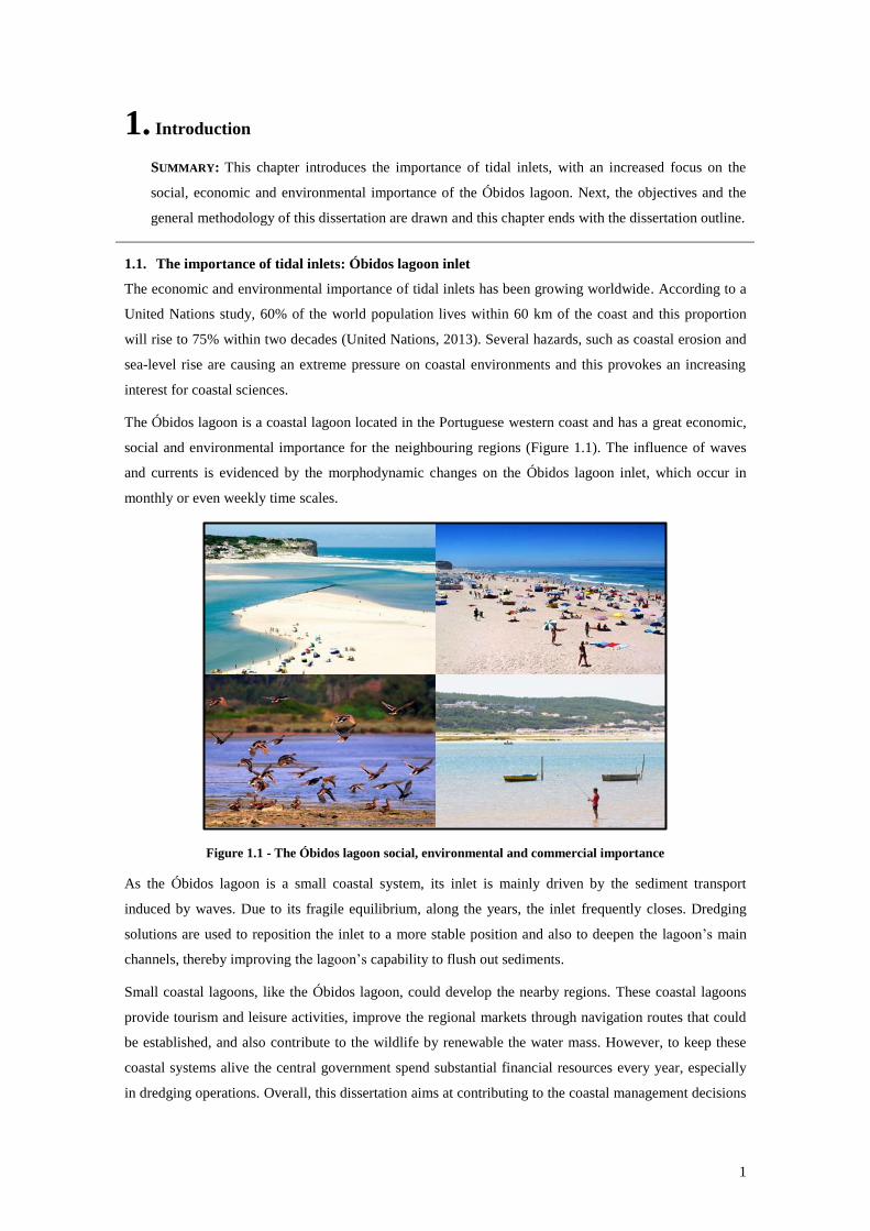
Figure 1.1 - The Óbidos lagoon social, environmental and commercial importance ................................... 1
Figure 2.1 - Morphological units of an inlet (adapted from Boothroyd, 1985) ............................................ 5
Figure 2.2 - Hubbard et al. (1979) inlet classification (adapted from Hayes and FitzGerald,
2013) ...................................................................................................................................... 7
Figure 2.3 - Hayes (1979) inlet classification (adapted from Hayes, 1979) ................................................. 7
Figure 2.4 - Escoffier (1977) stability diagram for inlets (adapted from Escoffier, 1977) ........................... 8
Figure 2.5 - Conceptual morphodynamic models (adapted from FitzGerald et al., 2000) ........................... 9
Figure 2.6 - Conceptual morphodynamic models (adapted from FitzGerald et al., 2000) ......................... 10
Figure 2.7 - Morphodynamic numerical scheme (adapted from Bertin et al., 2010).................................. 10
Figure 2.8 - A) Orthogonal structured grid; B) non-orthogonal curvilinear structured grid;
C) orthogonal curvilinear structured grid; D) unstructured grid (adapted from
Versteeg and Malalasekera, 2007) ....................................................................................... 11
Figure 2.9 – Geographical location of the Óbidos lagoon (green box) and its three main
tributaries (A, B and C in the blue box) (adapted from GoogleEarth) ................................. 12
Figure 2.10 – Distinct morphological zones in Óbidos lagoon: the upper (green box) and
lower zones (blue box) (adapted from GoogleEarth) .......................................................... 13
Figure 2.11 - Óbidos lagoon evolution in the last 5000 years (adapted from Ferreira et al.
2009) .................................................................................................................................... 14
Figure 2.12 – Three possible configurations of the inlet (adapted from Bruneau et al. 2011) ................... 15
Figure 2.13 – Zoom in on the Óbidos lagoon inlet of the area covered by the POOC (shaded
zone) (adapted from Consulmar, 2008) ............................................................................... 15
Figure 2.14 - Available Óbidos Lagoon morphological evolution since 1999 to present day
(adapted from Landstat) ....................................................................................................... 16
Figure 2.15 - Solution proposed by Fortunato and Oliveira (2007) ........................................................... 17
Figure 3.1 - Numerical scheme for model verification (adapted from Dodet, 2013) ................................. 20
Figure 3.2 - A - Spatial values of the Manning coefficient (m-1/3
s) according to Bruneau et
al. (2011); B - Extension of the Manning coefficient seawards ........................................... 21
Figure 3.3 – Reference levels for the Óbidos lagoon ................................................................................. 22
Figure 3.4 - Unstructured grid for the numerical model, bathymetry measured in July 2001,
wave gauge (black star), tidal gauges (yellow stars), open boundary nodes
(white crosses) and WW3 spectra points (white stars) (adapted from Google
Earth) ................................................................................................................................... 23
Figure 3.5 - Locations of the recorded model stations 1, 2, 3 and 4 (red stars from left to
right) for the sensitivity analysis, station for wave blocking phenomenon
verification (black star), bathymetry measured in July 2001 and simulated
scenarios to study the influence of different wave parameters inside Óbidos
lagoon .................................................................................................................................. 25
Figure 3.6 - Comparison between the model (red line) and data (blue line) for the time
period between 4 July 2001 and 21 October 2001 at the maritime station .......................... 26
II
Figure 3.7 - Model (red lines) and data (blue lines) SSE and MSL (dash lines) for Cais do
Arelho (top), Braço da Barrosa (middle) and Bico dos Corvos (bottom) from
18/07/2001 to 06/08/2001 referred to MSL ......................................................................... 27
Figure 3.8 - Top: SSE for a simulation without waves in front of the inlet (purple star in
Figure 3.11); Bottom: Differences on SSE for simulations with and without
the full interaction between waves and currents for the four stations in Figure
3.5 ........................................................................................................................................ 28
Figure 3.9 - Top: SSE for a simulation without waves in front of the inlet (purple star in
Figure 3.11); Bottom: Differences on SSE when comparing with a simulation
without waves ...................................................................................................................... 28
Figure 3.10 - Top: Hs at 5 m depth (black star in Figure 3.11); Middle: SSE for a simulation
without waves in front of the inlet (purple star in Figure 3.11); Bottom:
Differences on SSE when comparing with a simulation without waves
(Station 4) ............................................................................................................................ 29
Figure 3.11 - Hs for a JONSWAP spectrum with constant Hs (2,0 m) and Dir (315º N) as
forcing parameters ............................................................................................................... 30
Figure 3.12 - Top: Hs at 10 m depth (black star in Figure 3.13); Middle: SSE for a
simulation without waves in front of the inlet (purple star in Figure 3.11);
Bottom: Differences on SSE when compared with a simulation without
waves (Station 4).................................................................................................................. 31
Figure 3.13 - Hs for a JONSWAP spectrum with constant Hs (2,0 m) and Tp (9 s) as
forcing parameters ............................................................................................................... 31
Figure 3.14 – Comparison between a simulation with the full wave-current interaction (red
lines) and without (blue lines) for the Hs (first box), SSE (second box),
depth-average horizontal velocities (third box), Urms (fourth box) and
sediment discharge (fifth box) between the third and fourth days on the black
star (Figure 3.5) .................................................................................................................... 32
Figure 4.1 – Gradient of wave radiation stresses (left), barotropic pressure gradient forces
(center) and resultant forces (right) at the Óbidos lagoon inlet for shore-
normal waves of Hs = 3,0 m (adapted from Bertin et al., 2009a) ........................................ 36
Figure 4.2 – Morphodynamic numerical scheme (adapted from Dodet, 2013) .......................................... 37
Figure 4.3 – Spatial distribution of the median grain diameter – d50 (m) ................................................... 39
Figure 4.4 - Comparison between the initial (left) and the changed (right) bathymetry on the
northern margin .................................................................................................................... 40
Figure 4.5 – A – Simulated bathymetry at the end of November; B – Measured bathymetry
during November; C- Initial bathymetry in July 2001; Statistical error
measures............................................................................................................................... 42
Figure 4.6 –Morphodynamic evolution of the Óbidos lagoon between July and November
2001 for DP1 ........................................................................................................................ 43
III
Figure 4.7 – Evolution of the M2 amplitude in Cais do Arelho from July to November 2001
(adapted from Bertin et al., 2009a) ...................................................................................... 44
Figure 4.8 – Qualitative comparison between the DP1 (left) and the DP2 (right) at the end
of November 2001 ............................................................................................................... 44
Figure 4.9 - Qualitative comparison between the DP1 (left) and the DP3 (right) at the end
of November 2001 ............................................................................................................... 45
Figure 4.10 – Tidal prism of DP1 (black line), DP2 (red line) and DP3 (blue line) from July
to November 2001................................................................................................................ 45
Figure 4.11 – Ratio between the tidal prism of the DP2 (red lines) and the DP3 (blue lines)
with the tidal prism of the DP1 and the linear regression analysis for DP2 and
DP3 (strong lines) with the respective coefficients. ............................................................. 46
Figure 4.12 - Difference in ebb-flood durations near Cais do Arelho for the DP1 (black
line), the DP2 (red line) and the DP3 (blue line) from July to November 2001 .................. 47
Figure 4.13 - Difference in ebb-flood durations inside the lagoon (blue star in Figure 4.8)
for the DP1 (black line), the DP2 (red line) and the DP3 (blue line) from July
to November 2001................................................................................................................ 47
Figure 4.14 - Differences between the initial and 5 month simulated bathymetries for the
DP1 (left) and the DP2 (right) and the sediment volumes that crossed the
inlet (x104 m
3) ...................................................................................................................... 48
Figure 4.15 – Differences between the initial and 5 month simulated bathymetries for the
DP1 (left) and the DP3 (right) and the sediment volumes that crossed the
inlet (x104 m
3) ...................................................................................................................... 48
Figure 4.16 – Tidal prism-cross-section relationships for the three dredging plans ................................... 50
Figure 4.17 – Escoffier (1977) diagram for each dredging plan ................................................................. 51
Figure 5.1 – Conclusions scheme of chapter 3 ........................................................................................... 55
Figure 5.2 – Conclusions scheme of chapter 4 ........................................................................................... 56

V
LIST OF TABLES
Table 2.1 - Bruun and Gerritsen (1960) inlet stability criterion (adapted from Bruun and
Gerritsen, 1960) ........................................................................................................................ 8
Table 2.2 – Mean grain diameter (d50) and gradation coefficient (σD) in the Óbidos lagoon
(adapted from Fortunato et al., 2011) ..................................................................................... 13
Table 3.1 - Wave breaking type analysis based on the surf similarity parameter varying the
Tp ............................................................................................................................................ 29
Table 4.1 – Average differences between ebb and flood durations for two points inside the
Óbidos lagoon ......................................................................................................................... 47
Table 4.2 - Differences between ebb and flood durations for the initial and final
bathymetries and for each dredging plan ................................................................................ 49
Table 4.3 – Ratios between the sediment fluxes integrated in half of the tidal cycle (ebb or
flood) and in the inlet cross-section of DP2 and DP3 by DP1 for the initial and
final bathymetries ................................................................................................................... 50
Table 4.4 - Bruun and Gerritsen (1960) stability criterion application to the three dredging
plans ........................................................................................................................................ 52


VII
LIST OF SYMBOLS
AC Area of the inlet cross-section (m2)
Ani Area of the grid element i (m2)
c Wave celerity (m/s)
Cb Empirical coefficient of the linear JONSWAP parameterization (m2/s
3)
CD Drag coefficient computed from a Manning formulation (-)
cg Wave group velocity (m/s)
Ci Coefficient of the node i for the finite element method formulation (-)
cp Wave phase velocity (m/s)
CPA Empirical coefficient of the PA relationship (O’Brien, 1966) (-)
d50 Median grain diameter (m)
Dir Mean wave direction (º)
E Variance density of the sea level elevations (m2/Hz)
f Coriolis factor (-)
h Water depth (m)
H Total water depth (m)
H0 Offshore wave height (m)
Hs Significant wave height (m)
k Wave number (rad/s)
L Wavelength (m)
L0 Offshore wavelength (m)
m Coordinate perpendicular to the wave propagation direction (-)
Me Mobility parameter (Van Rijn, 2007) (-)
Mtot Gross annual littoral drift m3/year
N Wave action density (m2/(radHz
2))
n Empirical coefficient of the PA relationship (O’Brien, 1966) (-)
n0 Manning coefficient (n0=1/KS) (m-1/3
s)
P Tidal prism (m3)
q Depth-integrated volumetric sediment flux (m3/s/m)
Q Sediment transport rate integrated in time (m3/m)
Q*
Modified sediment transport rate integrated in time (m3/m)
qb Bedload sediment transport (Van Rijn, 2007a) (kg/m/s)
qs Suspended sediment transport (Van Rijn, 2007b) (kg/m/s)
qtot Total sediment transport (Soulsby, 1997) (kg/m/s)
Qx Sediment fluxes along x-direction (m3/m/s)
Qy Sediment fluxes along y-direction (m3/m/s)
s Coordinate along the wave propagation direction (-)
Sij Component of the radiation stress tensor in plan i along j direction (N/m2/m)
VIII
T Wave period (s)
Tp Wave peak period (s)
u Depth-average horizontal velocity along the x-axis (m/s)
UA Effective advection velocity (m/s)
ucr,c Critical velocity for currents (m/s)
ucr,w Critical velocity for waves (m/s)
ue Effective velocity (m/s)
Ui Average flow velocity at the inlet (m/s)
Urms Wave orbital velocity (m/s)
Uw Peak orbital velocity (m/s)
v Depth-average horizontal velocity along the y-axis (m/s)
Vm Maximum velocity on the transitional channel (Escoffier, 1977) (m/s)
Vtot Net balance of sediments through the inlet over a specific time period (m3)
Vtot_neg Total volume of sediments eroded inside the lagoon (m3)
Vtot_pos Total volume of sediments accreted inside the lagoon (m3)
X Cartesian coordinate vector (x,y) (m)
Greek symbols
β Beach slope for the Irribaren number (-)
βSVR97 Bed slope (Soulsby, 1997) (-)
γ Breaker height to water depth ratio (-)
Γi Length of the boundary element i (m)
Δh Bed update (m)
ε Diffusion coefficient for the modified Exner equation (-)
η Sea surface elevation (m)
θ Wave direction (º)
λ Porosity (-)
μ Horizontal eddy viscosity (m2/s)
ξ0 Irribaren number or surf similarity parameter (-)
ρ0 Water specific mass (kg/m3)
σ Wave relative frequency (rad/s)
σD Gradation coefficient (-)
τb Bottom shear stress (N/m2)
ω Wave absolute frequency (rad/s)
Ωi Control volume of the element i (m3)

IX
LIST OF ACRONYMS
ADCP Acoustic Doppler current profiler
BSS Brier-skill score
DAHV Depth-averaged horizontal velocities
DP1 Dreging plan proposed by DHI (1997)
DP2 Dredging plan proposed by Fortunato and Oliveira (2007)
DP3 Dredging plan proposed by Fortunato and Oliveira (2007) with only one transverse channel
FIBWC Full interaction between waves and currents
HZ Hydrographic zero
ME Mean error
MSL Mean sea level
RMSE Root-mean square error
SI Scatter index
Skill Skill error measure
SSE Sea surface elevations

1
1. Introduction
SUMMARY: This chapter introduces the importance of tidal inlets, with an increased focus on the
social, economic and environmental importance of the Óbidos lagoon. Next, the objectives and the
general methodology of this dissertation are drawn and this chapter ends with the dissertation outline.
1.1. The importance of tidal inlets: Óbidos lagoon inlet
The economic and environmental importance of tidal inlets has been growing worldwide. According to a
United Nations study, 60% of the world population lives within 60 km of the coast and this proportion
will rise to 75% within two decades (United Nations, 2013). Several hazards, such as coastal erosion and
sea-level rise are causing an extreme pressure on coastal environments and this provokes an increasing
interest for coastal sciences.
The Óbidos lagoon is a coastal lagoon located in the Portuguese western coast and has a great economic,
social and environmental importance for the neighbouring regions (Figure 1.1). The influence of waves
and currents is evidenced by the morphodynamic changes on the Óbidos lagoon inlet, which occur in
monthly or even weekly time scales.
Figure 1.1 - The Óbidos lagoon social, environmental and commercial importance
As the Óbidos lagoon is a small coastal system, its inlet is mainly driven by the sediment transport
induced by waves. Due to its fragile equilibrium, along the years, the inlet frequently closes. Dredging
solutions are used to reposition the inlet to a more stable position and also to deepen the lagoon’s main
channels, thereby improving the lagoon’s capability to flush out sediments.
Small coastal lagoons, like the Óbidos lagoon, could develop the nearby regions. These coastal lagoons
provide tourism and leisure activities, improve the regional markets through navigation routes that could
be established, and also contribute to the wildlife by renewable the water mass. However, to keep these
coastal systems alive the central government spend substantial financial resources every year, especially
in dredging operations. Overall, this dissertation aims at contributing to the coastal management decisions
2
that are most needed, with a major focus on the hydrodynamics and morphodynamics of the Óbidos
lagoon.
1.2. Objectives and general methodology
This dissertation has the following objectives:
1) To further investigate the effect of waves on the Óbidos lagoon hydrodynamics.
2) To verify the changes induced by the interactions between waves and currents on the sediments of
the Óbidos lagoon inlet.
3) To assess the morphodynamic changes induced by three different dredging plans on the
hydrodynamic behaviour and on the morphological evolution of the Óbidos lagoon.
4) To evaluate the impact of adding transverse channels in dredging plans.
To achieve the previous goals the following methodology is carried out:
1) A brief review of tidal inlets regarding inlet’s morphological units, classifications, stability and
conceptual or numerical morphodynamic models to provide the required theoretical background.
2) The presentation of the case under study - Óbidos lagoon – with a focus on tidal conditions, wave
regime, sediment characteristics, long and short term evolution and previous implemented
engineering solutions.
3) The validation of a coupled wave-circulation model with the data recorded by tidal gauges and an
acoustic Doppler current profiler (ADCP).
4) An analysis of the wave parameters effect on the Óbidos lagoon hydrodynamics and the importance
of the full interaction between wave and currents in the numerical model to sediment dynamics
through idealized wave conditions.
5) The calibration and verification of the morphodynamic model with the measured bathymetry.
6) The assessment of three different dredging plans during a period of five months with the
morphodynamic model.
7) The calculation of several parameters, such as tidal prism, differences between ebb and flood
durations, sediment fluxes that crossed the inlet, application of empirical stability relationships and
differences between initial and final bathymetries.
1.3. Outline of the dissertation
This dissertation is divided into five chapters including this Introduction. In chapter 2 a background
review is made. A number of concepts and definitions regarding tidal inlets are introduced like the tidal
prism, an inlet’s classifications and the role of stability. Associated with previous studies, conceptual and
numerical morphodynamic models are also described. Furthermore, the study area – the Óbidos lagoon -
is introduced and a full description of the past solutions that were implemented or studied in the last 20
years for the Óbidos lagoon is presented.
Chapter 3 studies the hydrodynamics of the Óbidos lagoon. In this chapter, the coupling between the
hydrodynamic and the wave model is verified and further exploited to understand the impact of the mean
wave direction on the sea surface elevations (SSE) inside the Óbidos lagoon. The wave blocking
phenomenon is also shown in this chapter.

3
The full morphodynamic model is verified in chapter 4. This verification involves a comparison with
measurements, and the good accuracy makes the morphodynamic model an appropriate tool to study the
evolution of the Óbidos lagoon inlet with different dredging plans and also, to investigate the impact of
transverse channels on the morphodynamics of the Óbidos lagoon inlet. Finally, chapter 5 presents the
main conclusions and some future work directions for subsequent studies are proposed.

5
2. Tidal inlets brief background review and the case study: the Óbidos lagoon
SUMMARY: This chapter introduces the theoretical background needed to perform the study of tidal
inlets. The morphological components of tidal inlets are introduced, a review on inlet’s
classifications and stability is made and some conceptual/numerical morphodynamic models are
presented. Next, the Óbidos lagoon relevant characteristics are described, such as, the wave regime,
tidal conditions and the median grain size spatial location. This chapter closes with a review on the
engineering solutions implemented and studied for this lagoon during the last twenty years.
2.1. Tidal inlets
2.1.1. Inlet morphological components
Tidal currents and waves shape the sediment deposits that constitute the morphological units of an inlet.
A tidal inlet corresponds to the transitional channel that connects an estuary or a costal lagoon to the sea.
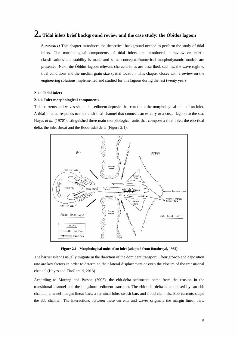
Hayes et al. (1970) distinguished three main morphological units that compose a tidal inlet: the ebb-tidal
delta, the inlet throat and the flood-tidal delta (Figure 2.1).
Figure 2.1 - Morphological units of an inlet (adapted from Boothroyd, 1985)
The barrier islands usually migrate in the direction of the dominant transport. Their growth and deposition
rate are key factors in order to determine their lateral displacement or even the closure of the transitional
channel (Hayes and FitzGerald, 2013).
According to Morang and Parson (2002), the ebb-delta sediments come from the erosion in the
transitional channel and the longshore sediment transport. The ebb-tidal delta is composed by: an ebb
channel, channel margin linear bars, a terminal lobe, swash bars and flood channels. Ebb currents shape
the ebb channel. The interactions between these currents and waves originate the margin linear bars.
6
When water leaves the ebb channel, the velocity decreases at the end of the terminal lobe and the
deposition of suspended sediments occurs. Wave-induced currents originate the movements of swash bars
between the terminal lobe and the ebb channel.
The flood-tidal delta is composed by four elements: flood ramp, flood channels, ebb shield and ebb spits.
Flood currents generate the flood ramp and the flood channels. The ebb shield induces the divergence of
these currents at the upstream end of the flood delta. The effect of both flood and ebb currents across the
margins generates ebb spits.
The bedforms found in the inlets are ripples, dunes and antidunes. The oscillatory motion induced by
waves in the inlets promotes the appearance of ripples, while dunes and antidunes are due to tidal
currents.
To study the tidal inlet morphodynamics it is necessary to introduce the concept of tidal prism. This
concept corresponds to the volume of water that crosses an inlet during a flood or ebb cycle (Equation
2.1)
𝑷 = ∫ 𝑼𝒊𝑨𝑪 𝒅𝒕𝐭𝟐
𝐭𝟏 [2.1]
where 𝑃 is the tidal prism and Ui is the average flow velocity at the inlet. Ac is the area of the inlet cross-
section and t1 and t2 are the temporal limits of the half tidal cycle period. Since the inlets have a dynamic
behaviour, changing in space and time, their tidal prism is also variable. Therefore, the tidal prism
depends on the inlet geometry, the wave forcing, the tidal amplitude and the area of the lagoon (O'Brien,
1966).
According to O'Brien (1966), the tidal prism of a spring tide is roughly proportional to the minimum
cross-section of the inlet. Walton and Adams (1976) show that there is a relationship between the tidal
prism of an inlet and the size of the ebb delta. FitzGerald (1988) stated that the volume of sand in the
flood and ebb deltas is comparable with the volume of sand in the adjacent barrier islands. According to
Nummedal and Fischer (1978), the geometry of the inlet entrance and its deltas depends on four factors:
the tidal amplitude, the wave energy along the coast, the bathymetry of the sand bar and the area of the
coastal lagoon.
2.1.2. Inlet classification and stability
A review of the specialized literature on tidal inlets shows that there are different classifications for this
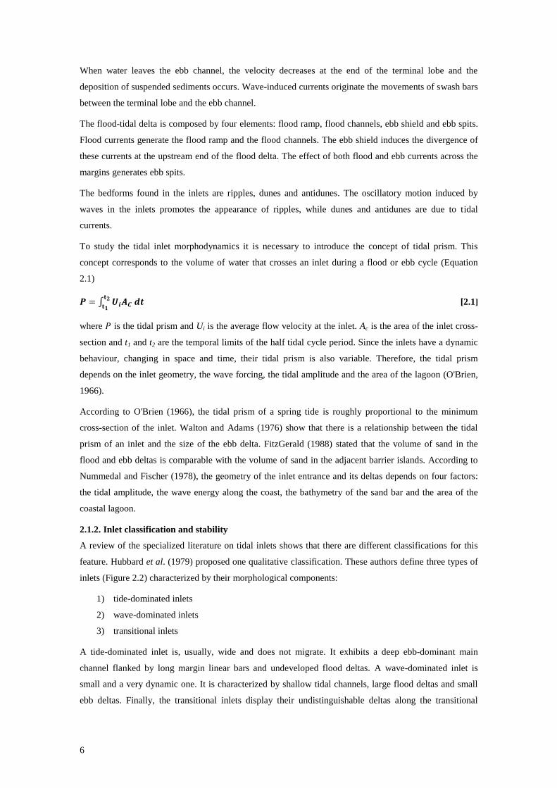
feature. Hubbard et al. (1979) proposed one qualitative classification. These authors define three types of
inlets (Figure 2.2) characterized by their morphological components:
1) tide-dominated inlets
2) wave-dominated inlets
3) transitional inlets
A tide-dominated inlet is, usually, wide and does not migrate. It exhibits a deep ebb-dominant main
channel flanked by long margin linear bars and undeveloped flood deltas. A wave-dominated inlet is
small and a very dynamic one. It is characterized by shallow tidal channels, large flood deltas and small
ebb deltas. Finally, the transitional inlets display their undistinguishable deltas along the transitional
7
channel. However, the previous empirical classification disregards the hydrodynamic forces which inlets
are subjected to.
Figure 2.2 - Hubbard et al. (1979) inlet classification (adapted from Hayes and FitzGerald, 2013)
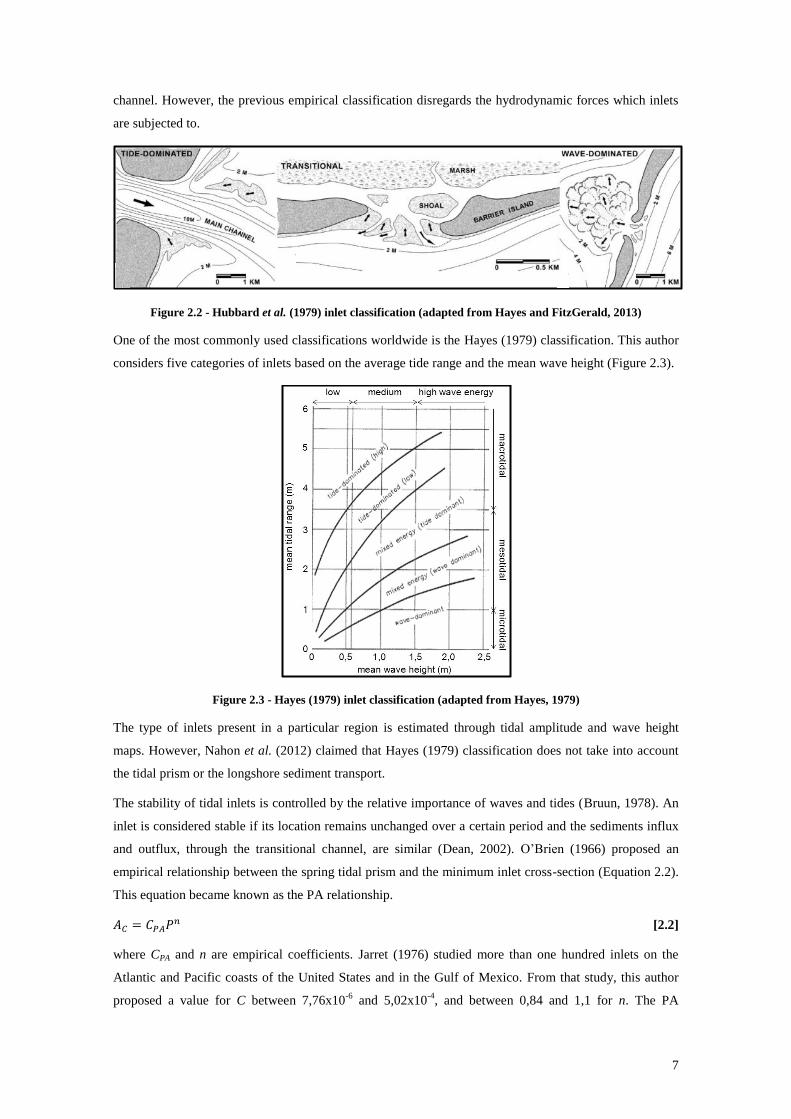
One of the most commonly used classifications worldwide is the Hayes (1979) classification. This author
considers five categories of inlets based on the average tide range and the mean wave height (Figure 2.3).
Figure 2.3 - Hayes (1979) inlet classification (adapted from Hayes, 1979)
The type of inlets present in a particular region is estimated through tidal amplitude and wave height
maps. However, Nahon et al. (2012) claimed that Hayes (1979) classification does not take into account
the tidal prism or the longshore sediment transport.
The stability of tidal inlets is controlled by the relative importance of waves and tides (Bruun, 1978). An
inlet is considered stable if its location remains unchanged over a certain period and the sediments influx
and outflux, through the transitional channel, are similar (Dean, 2002). O’Brien (1966) proposed an
empirical relationship between the spring tidal prism and the minimum inlet cross-section (Equation 2.2).
This equation became known as the PA relationship.
𝐴𝐶 = 𝐶𝑃𝐴𝑃𝑛 [2.2]
where CPA and n are empirical coefficients. Jarret (1976) studied more than one hundred inlets on the
Atlantic and Pacific coasts of the United States and in the Gulf of Mexico. From that study, this author
proposed a value for C between 7,76x10⁻⁶
and 5,02x10⁻⁴
, and between 0,84 and 1,1 for n. The PA

8
relationship has been demonstrated empirically and theoretically for tidal inlets in equilibrium. However,
Fortunato et al. (2014) have shown that the relationship is also valid for inlets that are away from
equilibrium.
Bruun and Gerritsen (1960) introduced the concept of tidal inlet global stability based on the ratio of the
tidal prism at spring tides and the gross annual littoral drift (Mtot) (Table 2.1). Nevertheless, this criterion
cannot be used to predict the evolution of an inlet with time-scales equal or lower to a year. According to
Dodet (2013) the reason for this lies in the Mtot, since it presents a strong inter-annual variability.
Table 2.1 - Bruun and Gerritsen (1960) inlet stability criterion (adapted from Bruun and Gerritsen, 1960)
Inlet Stability Ratings
𝑃 𝑀𝑡𝑜𝑡⁄ ≥ 150 Conditions are relatively good, little bar and good flushing
100 ≤ 𝑃 𝑀𝑡𝑜𝑡⁄ ≤ 150 Conditions become less satisfactory, and offshore bar formation becomes more
pronounced
50 ≤ 𝑃 𝑀𝑡𝑜𝑡⁄ ≤ 100 Entrance bar may be rather large, but there is usually a channel through the bar
20 ≤ 𝑃 𝑀𝑡𝑜𝑡⁄ ≤ 50 All inlets are typical “bar-bypassers”
𝑃 𝑀𝑡𝑜𝑡⁄ ≤ 20 Descriptive of cases where the entrances become unstable “overflow channels”
rather than permanent inlets
Escoffier (1977) considered that the stability of an inlet depends on the balance between settling and
erosion forces. This idea was developed analytically and relates the maximum velocity on the transitional
channel, Vm, with the area of the inlet cross-section, AC (Figure 2.4).
Figure 2.4 - Escoffier (1977) stability diagram for inlets (adapted from Escoffier, 1977)
The tails in the above diagram represent two distinct situations. The maximum velocity tends to zero and
the area of the inlet cross-section decreases (left tail) or the maximum velocity decreases as the cross-
section area increases (right tail). The first situation is mainly due to friction forces from the bottom and
side walls and the second one is the result of mass conservation for an arbitrary tidal prism.
There are two equilibrium points (1 and 2 in Figure 2.4). Point 1 is considered stable because if the area
increases the maximum velocity decreases and sediments deposition occurs until the equilibrium state is
reached. On the contrary, if the area decreases the maximum velocity will increase eroding sediments,
and driving the inlet back to the equilibrium situation. Point 2 is considered unstable because a decrease
of the area reduces the velocity inducing the inlet closure.
1
2
9
2.1.3. Morphodynamic models for tidal inlets – some examples
The first models which study tidal inlets were conceptual and based on observations. Brunn and Gerritsen
(1959) describe three mechanisms of sand bypassing through an inlet. The transport induced by waves
through the terminal lobe, the transport in the channels due to tidal currents and the transitional channel or
barrier islands migration.
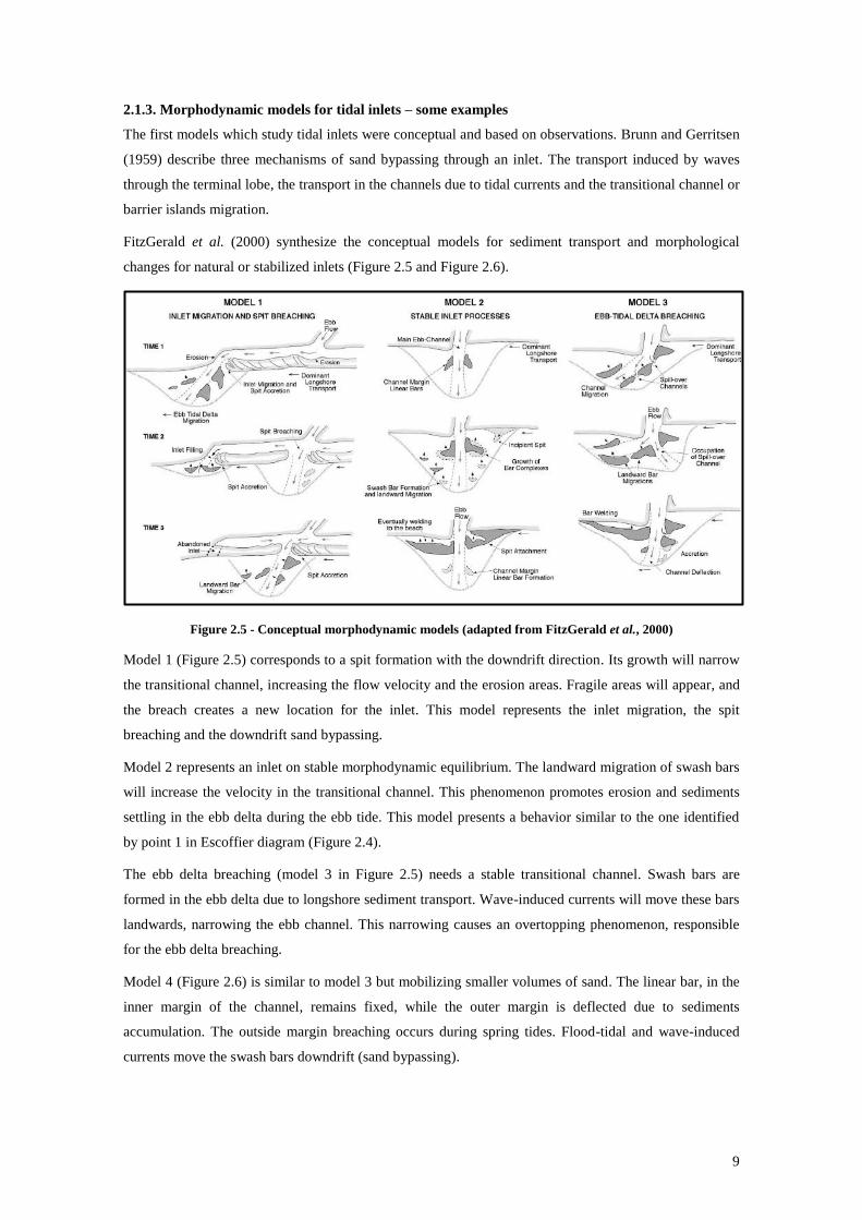
FitzGerald et al. (2000) synthesize the conceptual models for sediment transport and morphological
changes for natural or stabilized inlets (Figure 2.5 and Figure 2.6).
Figure 2.5 - Conceptual morphodynamic models (adapted from FitzGerald et al., 2000)
Model 1 (Figure 2.5) corresponds to a spit formation with the downdrift direction. Its growth will narrow
the transitional channel, increasing the flow velocity and the erosion areas. Fragile areas will appear, and
the breach creates a new location for the inlet. This model represents the inlet migration, the spit
breaching and the downdrift sand bypassing.
Model 2 represents an inlet on stable morphodynamic equilibrium. The landward migration of swash bars
will increase the velocity in the transitional channel. This phenomenon promotes erosion and sediments
settling in the ebb delta during the ebb tide. This model presents a behavior similar to the one identified
by point 1 in Escoffier diagram (Figure 2.4).
The ebb delta breaching (model 3 in Figure 2.5) needs a stable transitional channel. Swash bars are
formed in the ebb delta due to longshore sediment transport. Wave-induced currents will move these bars
landwards, narrowing the ebb channel. This narrowing causes an overtopping phenomenon, responsible
for the ebb delta breaching.
Model 4 (Figure 2.6) is similar to model 3 but mobilizing smaller volumes of sand. The linear bar, in the
inner margin of the channel, remains fixed, while the outer margin is deflected due to sediments
accumulation. The outside margin breaching occurs during spring tides. Flood-tidal and wave-induced
currents move the swash bars downdrift (sand bypassing).
10
Figure 2.6 - Conceptual morphodynamic models (adapted from FitzGerald et al., 2000)
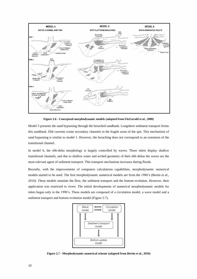
Model 5 presents the sand bypassing through the breached sandbank. Longshore sediment transport forms
this sandbank. Ebb currents create secondary channels in the fragile areas of the spit. This mechanism of
sand bypassing is similar to model 1. However, the breaching does not correspond to an extension of the
transitional channel.
In model 6, the ebb-delta morphology is largely controlled by waves. These inlets display shallow
transitional channels, and due to shallow water and arched geometry of their ebb deltas the waves are the
most relevant agent of sediment transport. This transport mechanism increases during floods.
Recently, with the improvements of computers calculations capabilities, morphodynamic numerical
models started to be used. The first morphodynamic numerical models are from the 1980’s (Bertin et al.,
2010). These models simulate the flow, the sediment transport and the bottom evolution. However, their
application was restricted to rivers. The initial developments of numerical morphodynamic models for
inlets began only in the 1990’s. These models are composed of a circulation model, a wave model and a
sediment transport and bottom evolution model (Figure 2.7).
Figure 2.7 - Morphodynamic numerical scheme (adapted from Bertin et al., 2010)

11
The grid is a fundamental component of numerical model and represents the spatial discretization of the
domain in analysis. The grids can be structured or unstructured (Figure 2.8). The grid used in this
dissertation is classified as unstructured. Unstructured grids are able to adapt to complex geometries in a
better way providing more flexibility for different resolutions.
Figure 2.8 - A) Orthogonal structured grid; B) non-orthogonal curvilinear structured grid; C) orthogonal
curvilinear structured grid; D) unstructured grid (adapted from Versteeg and Malalasekera, 2007)
Various morphodynamic models have been developed since the 1990’s. Mike-21 (Warren and Bach,
1992), Delft3D (Lesser et al., 2004), Morsys2D (Fortunato and Oliveira, 2004a; Bertin et al., 2009b),
Telemac&Sisyphe (Villaret et al., 2013) are examples of these developments. All these models can
simulate the morphodynamics of coastal zones.
Ranasinghe and Pattiaratchi (1999) applied a morphodynamic model to the Wilson inlet, in Australia. The
objective was to understand the physical processes responsible for the closing of the inlet and the
landward sediment transport constitutes the main mechanism that leads to the inlet’s closure. These
authors did not take into account the wave-current interaction due to the coupling incapability between
the models.
Cayocca (2001) studied the effect of tides and waves on the long-term morphodynamic changes in the
Arcachon inlet, France. This author was able to reproduce the opening of a new channel due to the tide.
Long-term morphodynamic simulations forced this author to use a representative tide and wave. The
representative tide and wave were obtained based on the annual sediment transport induced by tidal and
wave conditions.
Bertin et al. (2009a) used the Morsys2D model (Fortunato and Oliveira, 2004a; Bertin et al., 2009b) to
simulate the morphodynamics of the Óbidos lagoon inlet. The aim of this study was to understand the
relevant physical processes that occur near the inlet. The computational cost forced these authors to use a
2D model.
Villaret et al. (2013) coupled Telemac-2D and 3D (the hydrodynamic model) with Sisyphe (the sediment
transport and bottom evolution model) and applied them on curved channels, recirculating flows, sand
12
grading effects in a waterway and wave-induced littoral drift. These authors state that the main limitations
are due to the high degree of empiricism inherent in most sediment transport models.
Dodet (2013) applied a morphodynamic model (same as in this dissertation) to the Albufeira Lagoon.
This lagoon has an annual cyclic behavior and, in this study, the inlet was artificially opened in April and
closed in December. This author shows the importance of two sand transport mechanisms: the swash
transport and the infra-gravity wave transport. Until then, morphodynamic models neglected these two
mechanisms.
2.2. Study site - the Óbidos lagoon
2.2.1. Geomorphological and hydrodynamic settings of the Óbidos lagoon
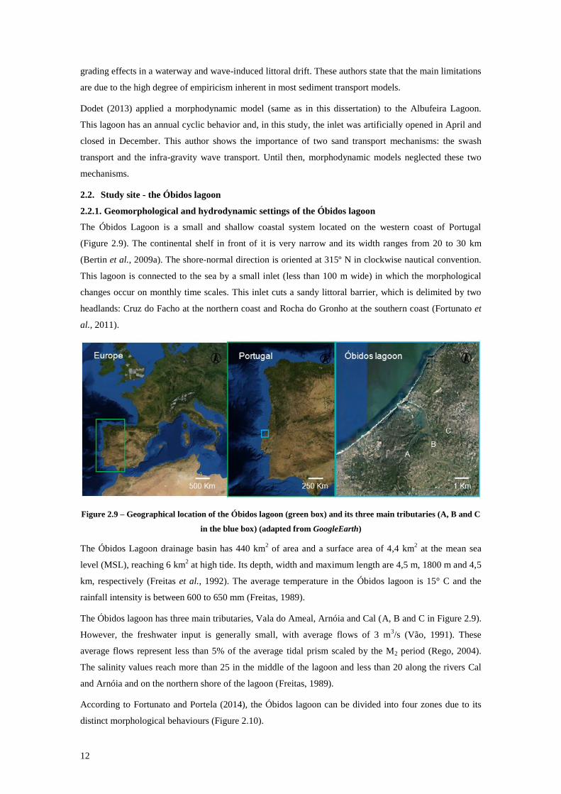
The Óbidos Lagoon is a small and shallow coastal system located on the western coast of Portugal
(Figure 2.9). The continental shelf in front of it is very narrow and its width ranges from 20 to 30 km
(Bertin et al., 2009a). The shore-normal direction is oriented at 315º N in clockwise nautical convention.
This lagoon is connected to the sea by a small inlet (less than 100 m wide) in which the morphological
changes occur on monthly time scales. This inlet cuts a sandy littoral barrier, which is delimited by two
headlands: Cruz do Facho at the northern coast and Rocha do Gronho at the southern coast (Fortunato et
al., 2011).
Figure 2.9 – Geographical location of the Óbidos lagoon (green box) and its three main tributaries (A, B and C
in the blue box) (adapted from GoogleEarth)
The Óbidos Lagoon drainage basin has 440 km2 of area and a surface area of 4,4 km
2 at the mean sea
level (MSL), reaching 6 km2 at high tide. Its depth, width and maximum length are 4,5 m, 1800 m and 4,5
km, respectively (Freitas et al., 1992). The average temperature in the Óbidos lagoon is 15° C and the
rainfall intensity is between 600 to 650 mm (Freitas, 1989).
The Óbidos lagoon has three main tributaries, Vala do Ameal, Arnóia and Cal (A, B and C in Figure 2.9).
However, the freshwater input is generally small, with average flows of 3 m3/s (Vão, 1991). These
average flows represent less than 5% of the average tidal prism scaled by the M2 period (Rego, 2004).
The salinity values reach more than 25 in the middle of the lagoon and less than 20 along the rivers Cal
and Arnóia and on the northern shore of the lagoon (Freitas, 1989).
According to Fortunato and Portela (2014), the Óbidos lagoon can be divided into four zones due to its
distinct morphological behaviours (Figure 2.10).
13
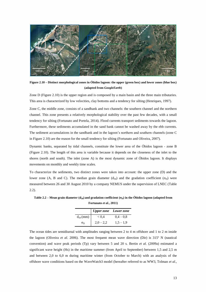
Figure 2.10 – Distinct morphological zones in Óbidos lagoon: the upper (green box) and lower zones (blue box)
(adapted from GoogleEarth)
Zone D (Figure 2.10) is the upper region and is composed by a main basin and the three main tributaries.
This area is characterized by low velocities, clay bottoms and a tendency for silting (Henriques, 1997).
Zone C, the middle zone, consists of a sandbank and two channels: the southern channel and the northern
channel. This zone presents a relatively morphological stability over the past few decades, with a small
tendency for silting (Fortunato and Portela, 2014). Flood currents transport sediments towards the lagoon.
Furthermore, these sediments accumulated in the sand bank cannot be washed away by the ebb currents.
The sediment accumulations in the sandbank and in the lagoon’s northern and southern channels (zone C
in Figure 2.10) are the reason for the small tendency for silting (Fortunato and Oliveira, 2007).
Dynamic banks, separated by tidal channels, constitute the lower area of the Óbidos lagoon - zone B
(Figure 2.10). The length of this area is variable because it depends on the closeness of the inlet to the
shores (north and south). The inlet (zone A) is the most dynamic zone of Óbidos lagoon. It displays
movements on monthly and weekly time scales.
To characterize the sediments, two distinct zones were taken into account: the upper zone (D) and the
lower zone (A, B and C). The median grain diameter (d50) and the gradation coefficient (σD) were
measured between 26 and 30 August 2010 by a company NEMUS under the supervision of LNEC (Table
2.2).
Table 2.2 – Mean grain diameter (d50) and gradation coefficient (σD) in the Óbidos lagoon (adapted from
Fortunato et al., 2011)
Upper zone Lower zone
d50 (mm) < 0,4 0,4 – 0,8
σD 2,0 – 2,2 1,5 – 1,9
The ocean tides are semidiurnal with amplitudes ranging between 2 to 4 m offshore and 1 to 2 m inside
the lagoon (Oliveira et al. 2006). The most frequent mean wave direction (Dir) is 315º N (nautical
convention) and wave peak periods (Tp) vary between 5 and 20 s. Bertin et al. (2009a) estimated a
significant wave height (Hs) in the maritime summer (from April to September) between 1,5 and 2,5 m
and between 2,0 to 6,0 m during maritime winter (from October to March) with an analysis of the
offshore wave conditions based on the WaveWatch3 model (hereafter referred to as WW3, Tolman et al.,
14
2002 and further developed by Dodet et al., 2010). Bruneau et al. (2011) based on the WW3 outputs also
estimated an extreme offshore wave climate and concluded that the wave height exceeds 2,5m 20% of the
time. According to the classification defined by Hayes (1979), the Óbidos lagoon inlet can be
characterized as a mixed-inlet dominated by tides in the maritime summer and a mixed-inlet dominated
by waves in the maritime winter. However, several authors characterized this inlet as a wave-dominated
inlet (Oliveira et al., 2006; Bertin et al., 2009a; Bruneau et al., 2011; Bertin et al., 2015) because the
wave-induced processes are very intense in the Óbidos lagoon inlet.
2.2.2. Long and short time scales of the morphosedimentary evolution
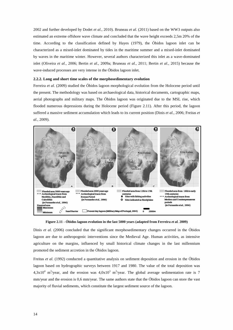
Ferreira et al. (2009) studied the Óbidos lagoon morphological evolution from the Holocene period until
the present. The methodology was based on archaeological data, historical documents, cartographic maps,
aerial photographs and military maps. The Óbidos lagoon was originated due to the MSL rise, which
flooded numerous depressions during the Holocene period (Figure 2.11). After this period, the lagoon
suffered a massive sediment accumulation which leads to its current position (Dinis et al., 2006; Freitas et
al., 2009).
Figure 2.11 - Óbidos lagoon evolution in the last 5000 years (adapted from Ferreira et al. 2009)
Dinis et al. (2006) concluded that the significant morphosedimentary changes occurred in the Óbidos
lagoon are due to anthropogenic interventions since the Medieval Age. Human activities, as intensive
agriculture on the margins, influenced by small historical climate changes in the last millennium
promoted the sediment accretion in the Óbidos lagoon.
Freitas et al. (1992) conducted a quantitative analysis on sediment deposition and erosion in the Óbidos
lagoon based on hydrographic surveys between 1917 and 1980. The value of the total deposition was
4,3x10⁴ m
3/year, and the erosion was 4,0x10
3 m
3/year. The global average sedimentation rate is 7
mm/year and the erosion is 0,6 mm/year. The same authors state that the Óbidos lagoon can store the vast
majority of fluvial sediments, which constitute the largest sediment source of the lagoon.
15
Fortunato et al. (2011) compared the bathymetries of the Óbidos lagoon between 2000 and 2004 in the
upper zone (zone D). The comparison area of the previous study was 2,6x10⁶ m
2 and these authors
concluded that the average sedimentation rate was 49 mm/year. This enhances the increased
sedimentation behaviour in the Óbidos lagoon along the recent years.
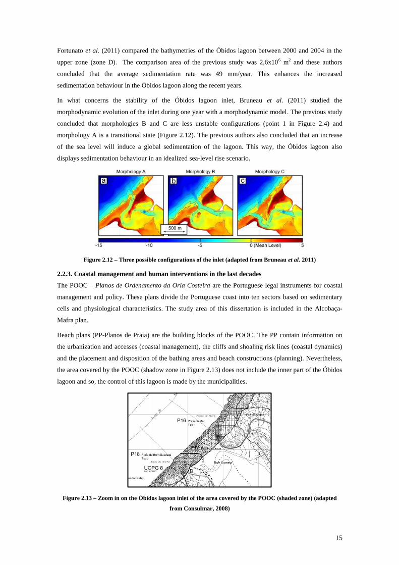
In what concerns the stability of the Óbidos lagoon inlet, Bruneau et al. (2011) studied the
morphodynamic evolution of the inlet during one year with a morphodynamic model. The previous study
concluded that morphologies B and C are less unstable configurations (point 1 in Figure 2.4) and
morphology A is a transitional state (Figure 2.12). The previous authors also concluded that an increase
of the sea level will induce a global sedimentation of the lagoon. This way, the Óbidos lagoon also
displays sedimentation behaviour in an idealized sea-level rise scenario.
Figure 2.12 – Three possible configurations of the inlet (adapted from Bruneau et al. 2011)
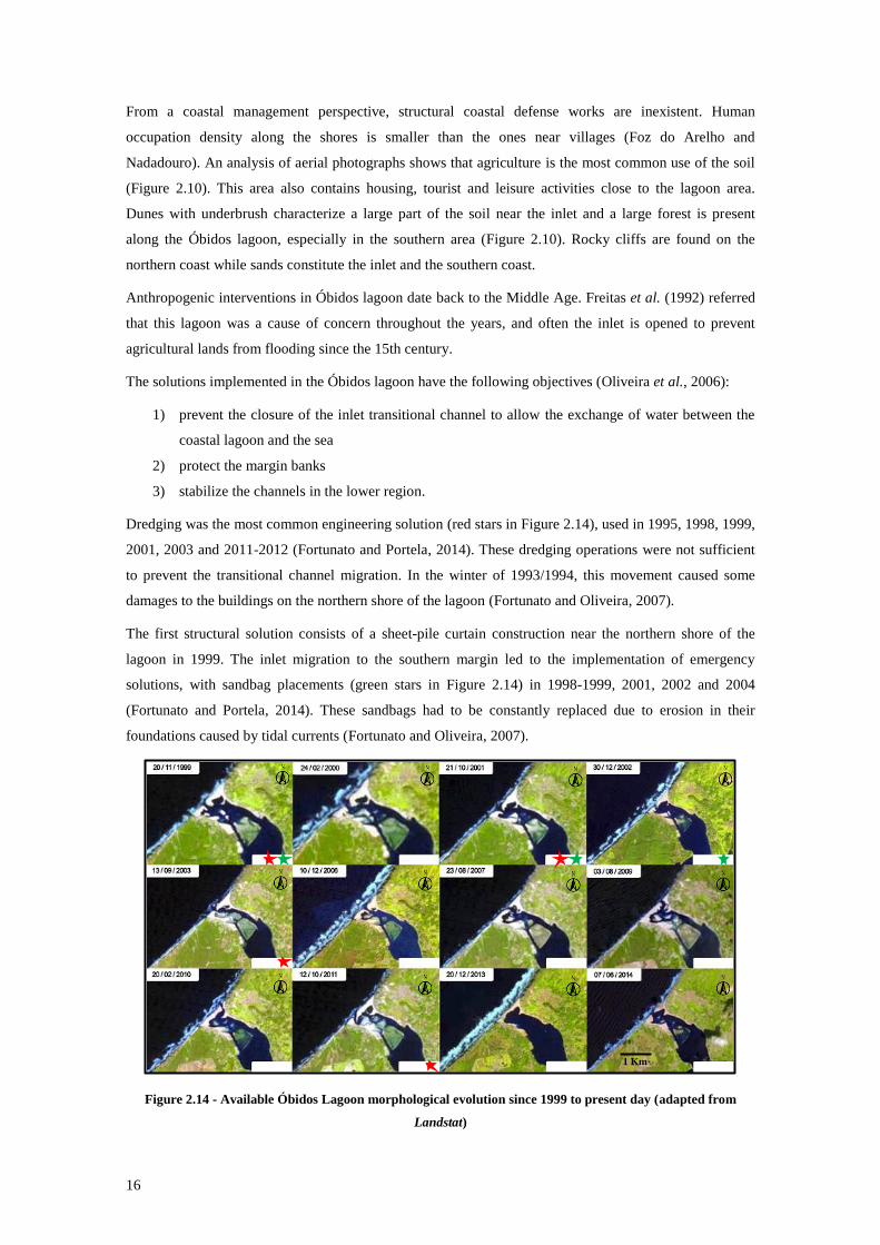
2.2.3. Coastal management and human interventions in the last decades
The POOC – Planos de Ordenamento da Orla Costeira are the Portuguese legal instruments for coastal
management and policy. These plans divide the Portuguese coast into ten sectors based on sedimentary
cells and physiological characteristics. The study area of this dissertation is included in the Alcobaça-
Mafra plan.
Beach plans (PP-Planos de Praia) are the building blocks of the POOC. The PP contain information on
the urbanization and accesses (coastal management), the cliffs and shoaling risk lines (coastal dynamics)
and the placement and disposition of the bathing areas and beach constructions (planning). Nevertheless,
the area covered by the POOC (shadow zone in Figure 2.13) does not include the inner part of the Óbidos
lagoon and so, the control of this lagoon is made by the municipalities.
Figure 2.13 – Zoom in on the Óbidos lagoon inlet of the area covered by the POOC (shaded zone) (adapted
from Consulmar, 2008)
16
From a coastal management perspective, structural coastal defense works are inexistent. Human
occupation density along the shores is smaller than the ones near villages (Foz do Arelho and
Nadadouro). An analysis of aerial photographs shows that agriculture is the most common use of the soil
(Figure 2.10). This area also contains housing, tourist and leisure activities close to the lagoon area.
Dunes with underbrush characterize a large part of the soil near the inlet and a large forest is present
along the Óbidos lagoon, especially in the southern area (Figure 2.10). Rocky cliffs are found on the
northern coast while sands constitute the inlet and the southern coast.
Anthropogenic interventions in Óbidos lagoon date back to the Middle Age. Freitas et al. (1992) referred
that this lagoon was a cause of concern throughout the years, and often the inlet is opened to prevent
agricultural lands from flooding since the 15th century.
The solutions implemented in the Óbidos lagoon have the following objectives (Oliveira et al., 2006):
1) prevent the closure of the inlet transitional channel to allow the exchange of water between the
coastal lagoon and the sea
2) protect the margin banks
3) stabilize the channels in the lower region.
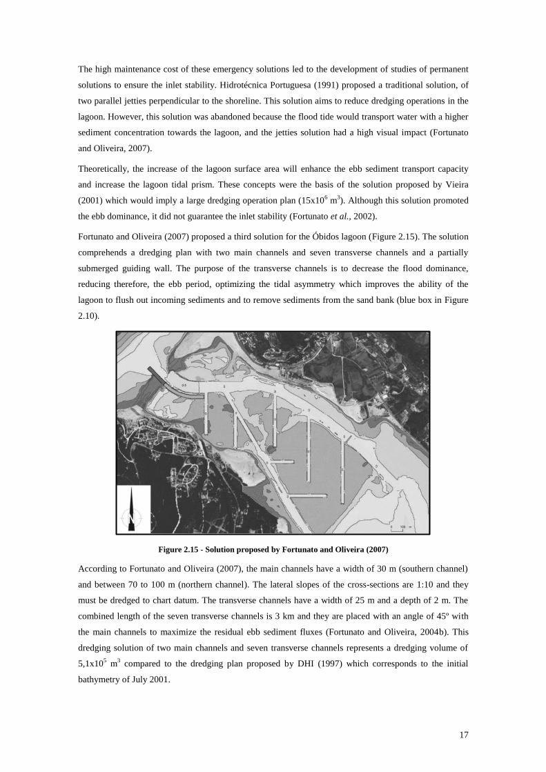
Dredging was the most common engineering solution (red stars in Figure 2.14), used in 1995, 1998, 1999,
2001, 2003 and 2011-2012 (Fortunato and Portela, 2014). These dredging operations were not sufficient
to prevent the transitional channel migration. In the winter of 1993/1994, this movement caused some
damages to the buildings on the northern shore of the lagoon (Fortunato and Oliveira, 2007).
The first structural solution consists of a sheet-pile curtain construction near the northern shore of the
lagoon in 1999. The inlet migration to the southern margin led to the implementation of emergency
solutions, with sandbag placements (green stars in Figure 2.14) in 1998-1999, 2001, 2002 and 2004
(Fortunato and Portela, 2014). These sandbags had to be constantly replaced due to erosion in their
foundations caused by tidal currents (Fortunato and Oliveira, 2007).
Figure 2.14 - Available Óbidos Lagoon morphological evolution since 1999 to present day (adapted from
Landstat)
1 Km
17
The high maintenance cost of these emergency solutions led to the development of studies of permanent
solutions to ensure the inlet stability. Hidrotécnica Portuguesa (1991) proposed a traditional solution, of
two parallel jetties perpendicular to the shoreline. This solution aims to reduce dredging operations in the
lagoon. However, this solution was abandoned because the flood tide would transport water with a higher
sediment concentration towards the lagoon, and the jetties solution had a high visual impact (Fortunato
and Oliveira, 2007).
Theoretically, the increase of the lagoon surface area will enhance the ebb sediment transport capacity
and increase the lagoon tidal prism. These concepts were the basis of the solution proposed by Vieira
(2001) which would imply a large dredging operation plan (15x106 m
3). Although this solution promoted
the ebb dominance, it did not guarantee the inlet stability (Fortunato et al., 2002).
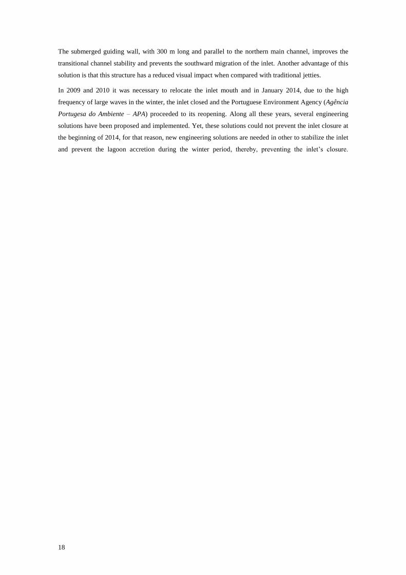
Fortunato and Oliveira (2007) proposed a third solution for the Óbidos lagoon (Figure 2.15). The solution
comprehends a dredging plan with two main channels and seven transverse channels and a partially
submerged guiding wall. The purpose of the transverse channels is to decrease the flood dominance,
reducing therefore, the ebb period, optimizing the tidal asymmetry which improves the ability of the
lagoon to flush out incoming sediments and to remove sediments from the sand bank (blue box in Figure
2.10).
Figure 2.15 - Solution proposed by Fortunato and Oliveira (2007)
According to Fortunato and Oliveira (2007), the main channels have a width of 30 m (southern channel)
and between 70 to 100 m (northern channel). The lateral slopes of the cross-sections are 1:10 and they
must be dredged to chart datum. The transverse channels have a width of 25 m and a depth of 2 m. The
combined length of the seven transverse channels is 3 km and they are placed with an angle of 45º with
the main channels to maximize the residual ebb sediment fluxes (Fortunato and Oliveira, 2004b). This
dredging solution of two main channels and seven transverse channels represents a dredging volume of
5,1x10⁵ m
3 compared to the dredging plan proposed by DHI (1997) which corresponds to the initial
bathymetry of July 2001.
18
The submerged guiding wall, with 300 m long and parallel to the northern main channel, improves the
transitional channel stability and prevents the southward migration of the inlet. Another advantage of this
solution is that this structure has a reduced visual impact when compared with traditional jetties.
In 2009 and 2010 it was necessary to relocate the inlet mouth and in January 2014, due to the high
frequency of large waves in the winter, the inlet closed and the Portuguese Environment Agency (Agência
Portugesa do Ambiente – APA) proceeded to its reopening. Along all these years, several engineering
solutions have been proposed and implemented. Yet, these solutions could not prevent the inlet closure at
the beginning of 2014, for that reason, new engineering solutions are needed in other to stabilize the inlet
and prevent the lagoon accretion during the winter period, thereby, preventing the inlet’s closure.
19
3. The influence of external forcing on the Óbidos lagoon hydrodynamics
SUMMARY: This chapter concerns the effect of waves on the sea surface elevations and on the
sediment dynamics in the Óbidos lagoon. To study the effect induced by waves, a fully coupled
hydrodynamic and wave model was used in order to simulate the water circulation taking into
account the wave-current interaction. The results of the following simulations are reported: sea
surface elevations inside the lagoon, significant wave heights in front of the inlet and sediment
discharge at the beginning of the flood delta. From these results, it was found that sea surface
elevations increased for the north-west mean wave direction. Also, the consideration of the full
interaction between waves and currents in the numerical model increased the sediment transport
towards the lagoon during the flood up to 30%.
3.1. Brief review on the effect of waves in the hydrodynamics of two Portuguese coastal lagoons
Atmospheric (wind and rain) and marine (tides and waves) forcings cause rapid changes in the physical
characteristics of coastal lagoons (Troussellier and Gattuso, 2007). The presence of waves can influence
the sea-level variations in a quite significant way (Nielsen and Apelt, 2003) and this rise on the sea level
due to waves is called “wave set-up”. Longuet-Higgins and Stewart (1960) relate this effect to the concept
of radiation stresses, which are defined as the excess of flow momentum due to the presence of waves.
It is known that the radiation stresses increase the MSL outside the Óbidos lagoon and this increase
outside propagates further inside (Malhadas et al., 2009, Bertin et al., 2009a). Also, a higher Hs will
increase the SSE on the Óbidos lagoon transitional channel, due to the dependency of the radiation
stresses on this variable. However, in what concerns Tp and Dir, the precise nature of their impact on the
SSE in the Óbidos lagoon remains an open issue.
Coastal inlets, such as Óbidos lagoon inlet, induce the lag and damping of the tidal signal and the
differences in the MSL, inside and outside the lagoon, produce tidal currents. The interaction between
tidal currents and waves leads to complex current fields at the inlet entrance and adjacent beaches.
Several wave experiments (Kemp and Simons, 1982, 1983; Klopman, 1994; Umeyama, 2005) and
numerical simulations (Groeneweg and Klopman, 1998; Olabarrieta et al., 2010; Teles et al., 2013) were
carried out to investigate the evolution of wave characteristics under the influence of currents.
Dodet et al. (2013) studied the wave-current interactions in the inlet of the Albufeira lagoon and
experienced the wave blocking phenomenon. The wave blocking phenomenon is the blocking of wave-
induced currents by the ebb currents. These authors found that if the wave model disregards wave-
currents interaction the Hs will not drop quickly inside the lagoon as they verified in data. Also, the
disregarding of this interaction attenuates the seaward sediment fluxes during the ebb. Therefore, this
chapter also aims to investigate the wave blocking phenomenon at the Óbidos lagoon.
3.2. Methodology - a two-way coupling between SELFE and WWM-II
3.2.1. General scheme
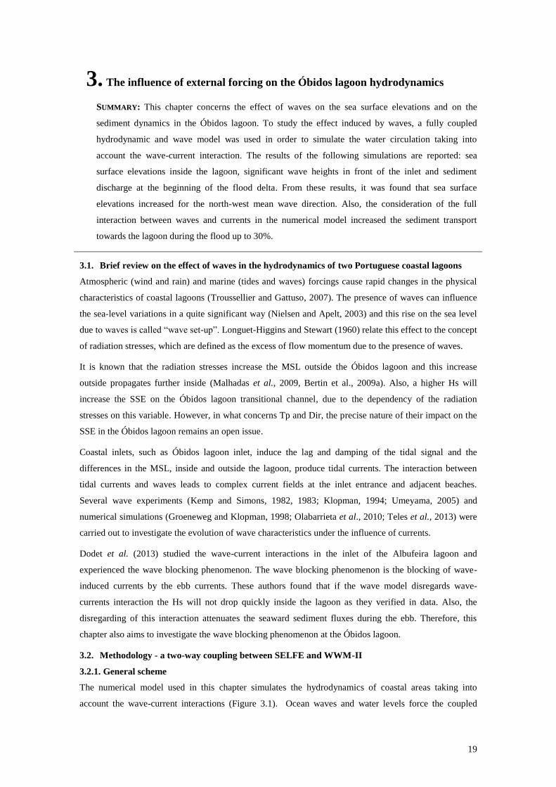
The numerical model used in this chapter simulates the hydrodynamics of coastal areas taking into
account the wave-current interactions (Figure 3.1). Ocean waves and water levels force the coupled
20
model at its boundaries. First, the wave model calculates the radiation stresses (𝑆𝑥𝑥, 𝑆𝑦𝑦 and 𝑆𝑦𝑥), which
will be the inputs for the circulation model. Then, the circulation model obtains the sea surface elevations
(𝜂) and the depth-averaged horizontal velocities (𝑢 and 𝑣). In the following time step, the wave model is
updated with the SSE and the currents from the circulation model and this iterative cycle continues until
an instant specified by the user.
Figure 3.1 - Numerical scheme for model verification (adapted from Dodet, 2013)
In this dissertation, the two models will be verified against an ADCP and tidal gauges measurements
recorded by the Portuguese Hydrographic Institute (IH, 2001) using the scheme of Figure 3.1. The
following step corresponds to a sensitivity analysis on the wave characteristics and for that reason, the
waves must be forced with a JONSWAP spectrum instead of the WW3 wave spectra. The wave blocking
phenomenon will be also addressed with a JONSWAP spectrum in order to specify constant wave
parameters (Hs, Tp and Dir) on the sea boundary.
3.2.2. The wave model – WWM-II
The spectral phase-averaged wave model WWM-II (Wind Wave Model II – Roland, 2009) solves the
wave action density balance equation and was coupled with SELFE in quasi-steady mode to propagate the
waves from the ocean to the coast. An explanation of the equations solved by WWM-II is presented in
APPENDIX A.
This wave model uses an unstructured grid and has a parallel processing system. This feature renders it
suitable to be coupled with SELFE, avoiding interpolation algorithms between structured and
unstructured meshes (e.g., Bertin et al., 2009a; Bruneau et al., 2011). There are two coupling options
between the models: the fully-coupled and partial coupled. The latter option causes the currents from
SELFE to be disregarded by WWM-II.
The spectral discretization was done according to 12 frequencies ranging from 0,2 and 0,05 Hz. The
directional discretization was done according to 12 directions in a window of 180º (0º - SW and 180º -
NE) with a resolution of 15º. WWM-II was set to take into account the bottom friction based on the
empirical JONSWAP parametrization (Hasselman et al., 1973) with the empirical coefficient Cb of 0,067
m2s
-3, the triad wave-wave interaction, the full interaction between waves and currents (fully-coupled)
and the dissipation by wave breaking with a constant wave breaking coefficient γ of 0,78.
In this dissertation the deep-water source-terms mechanisms (four-wave interaction, white capping and
wave generation by wind forcing) were disregarded because the domain of this study area is small (10
km). These simplifications reduced the computational time by approximately 20 to 30%.
21
Significant wave height, period, direction, wavelength and orbital velocity outputted from WWM-II were
used to compute gradients of radiation stresses to force the hydrodynamic model (SELFE). The radiation
stresses were computed from the classical formulation of Longuet-Higgings and Stewart (1964) with a
time step of 5 min, which is in accordance with Dodet (2013).
3.2.3. The hydrodynamic model - SELFE
The circulation model SELFE (Semi-implicit Eulerian-Lagrangian Finite Element model – Zhang and
Baptista, 2008) uses an unstructured grid in a parallel processing system. The unstructured grid allows
this numerical model to be suitable for estuaries and tidal inlets, ensuring flexibility for different scales
and resolutions. The configuration used in this dissertation was a 2D barotropic model with the
hydrostatic assumption and the Boussinesq approximation in Cartesian coordinates. SELFE solves the
2D shallow water equations trough a semi-implicit time stepping scheme and uses a finite-element
method for the spatial discretization. A review of the equations solved by SELFE is presented in
APPENDIX A.
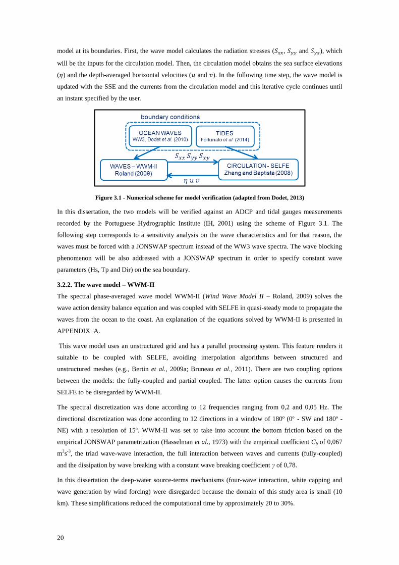
To account for bottom friction, a Manning coefficient (n0) variable in space was used in SELFE based on
the previous study of Bruneau et al. (2011) with a minor extension seawards (Figure 3.2) in order to
reduce the large velocity vectors that appeared during the ebb (APPENDIX B). The Manning
formulation threshold depth (variable H in Equation 17 - APPENDIX A) was set to 0,10 m. The water
depth threshold for drying was set on 0,01 m, which is in accordance with Dodet et al. (2013). To account
for horizontal turbulence, a constant horizontal eddy viscosity μ of 1 m2s
-1 was set in the entire domain.
The hydrodynamic time step was 20 s, producing outputs of sea surface elevations and velocities, saved
every 30 min over the domain.
Figure 3.2 - A - Spatial values of the Manning coefficient (m-1/3s) according to Bruneau et al. (2011); B -
Extension of the Manning coefficient seawards
3.2.4. Boundary conditions and numerical grid
The hydrodynamic model was forced at its ocean boundary (white crosses in Figure 3.4) by 20 tidal
constituents whose amplitude and phase were computed with the regional model of Fortunato et al.
A B
22
(2014). The atmospheric pressure remained constant (1015 HPa with a standard deviation of 3 HPa) along
the study period and the atmospheric pressure variations were disregarded (Bertin et al., 2009a).
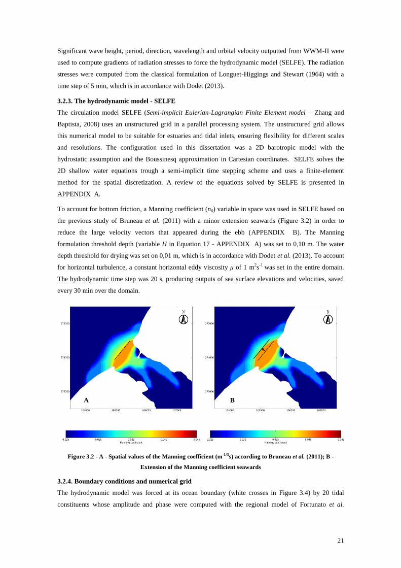
The upstream boundary in the lagoon was defined as a closed boundary since freshwater inflow is
negligible (section 2.2.1). The MSL increased over the last decades. In Cascais tidal gauge it can be
observed an increase of approximately 0,15 m relative to the hydrographic zero (HZ) since 1938, thereby,
the amplitude of the harmonic constituent M0 was set to 0,15 m. Finally, because the bathymetry was
related to the MSL and data was recorded to the HZ, 2 m were subtracted to the data measurements in
order to evaluate the results (Figure 3.3).
Figure 3.3 – Reference levels for the Óbidos lagoon
The offshore forcing was obtained from the previous study of Bruneau et al. (2011), provided by the
regional application of the WW3 model which gives the 2D wave spectrum in each WW3 spectra point
(white stars in Figure 3.4) with a time step of 3 h. The wave spectra are then linearly interpolated between
the spectra points and the ocean boundary nodes (white crosses in Figure 3.4).
The unstructured grid used by both models (Figure 3.4) had 57880 elements and 29398 nodes that were
set by previous studies (Bruneau et al., 2011). The spatial resolution of the grid ranges from 1,6 km (open
boundary) to 6 m (inlet).
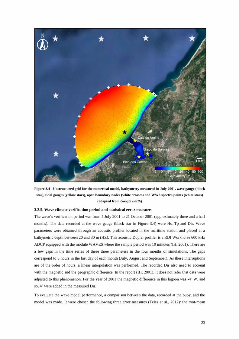
23
Figure 3.4 - Unstructured grid for the numerical model, bathymetry measured in July 2001, wave gauge (black
star), tidal gauges (yellow stars), open boundary nodes (white crosses) and WW3 spectra points (white stars)
(adapted from Google Earth)
3.2.5. Wave climate verification period and statistical error measures
The wave’s verification period was from 4 July 2001 to 21 October 2001 (approximately three and a half
months). The data recorded at the wave gauge (black star in Figure 3.4) were Hs, Tp and Dir. Wave
parameters were obtained through an acoustic profiler located in the maritime station and placed at a
bathymetric depth between 20 and 30 m (HZ). This acoustic Dopler profiler is a RDI Workhorse 600 kHz
ADCP equipped with the module WAVES where the sample period was 10 minutes (IH, 2001). There are
a few gaps in the time series of these three parameters in the four months of simulations. The gaps
correspond to 5 hours in the last day of each month (July, August and September). As these interruptions
are of the order of hours, a linear interpolation was performed. The recorded Dir also need to account
with the magnetic and the geographic difference. In the report (IH, 2001), it does not refer that data were
adjusted to this phenomenon. For the year of 2001 the magnetic difference in this lagoon was -4º W, and
so, 4º were added in the measured Dir.
To evaluate the wave model performance, a comparison between the data, recorded at the buoy, and the
model was made. It were chosen the following three error measures (Teles et al., 2012): the root-mean
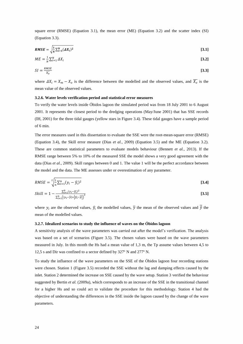
24
square error (RMSE) (Equation 3.1), the mean error (ME) (Equation 3.2) and the scatter index (SI)
(Equation 3.3).
𝑹𝑴𝑺𝑬 = √𝟏
𝑵∑ (𝜟𝑿𝒊)
𝟐𝑵𝒊=𝟏 [3.1]
𝑀𝐸 =1
𝑁∑ 𝛥𝑋𝑖
𝑁𝑖=1 [3.2]
𝑆𝐼 =𝑅𝑀𝑆𝐸
𝑋𝑜̅̅ ̅̅ [3.3]
where 𝛥𝑋𝑖 = 𝑋𝑚 − 𝑋𝑜 is the difference between the modelled and the observed values, and 𝑋𝑜̅̅ ̅ is the
mean value of the observed values.
3.2.6. Water levels verification period and statistical error measures
To verify the water levels inside Óbidos lagoon the simulated period was from 18 July 2001 to 6 August
2001. It represents the closest period to the dredging operations (May/June 2001) that has SSE records
(IH, 2001) for the three tidal gauges (yellow stars in Figure 3.4). These tidal gauges have a sample period
of 6 min.
The error measures used in this dissertation to evaluate the SSE were the root-mean-square error (RMSE)
(Equation 3.4), the Skill error measure (Dias et al., 2009) (Equation 3.5) and the ME (Equation 3.2).
These are common statistical parameters to evaluate models behaviour (Bennett et al., 2013). If the
RMSE range between 5% to 10% of the measured SSE the model shows a very good agreement with the
data (Dias et al., 2009). Skill ranges between 0 and 1. The value 1 will be the perfect accordance between
the model and the data. The ME assesses under or overestimation of any parameter.
𝑅𝑀𝑆𝐸 = √1
𝑛∑ (𝑦𝑖 − 𝑦�̂�)
2𝑛𝑖=1
2 [3.4]
𝑆𝑘𝑖𝑙𝑙 = 1 −∑ (𝑦𝑖−𝑦�̂�)2𝑛
𝑖=1
∑ (|𝑦𝑖−𝑦|+|𝑦�̂�−�̂�|)2
𝑛𝑖=1
[3.5]
where 𝑦𝑖 are the observed values, 𝑦�̂� the modelled values, 𝑦 the mean of the observed values and �̂� the
mean of the modelled values.
3.2.7. Idealized scenarios to study the influence of waves on the Óbidos lagoon
A sensitivity analysis of the wave parameters was carried out after the model’s verification. The analysis
was based on a set of scenarios (Figure 3.5). The chosen values were based on the wave parameters
measured in July. In this month the Hs had a mean value of 1,3 m, the Tp assume values between 4,5 to
12,5 s and Dir was confined to a sector defined by 327º N and 277º N.
To study the influence of the wave parameters on the SSE of the Óbidos lagoon four recording stations
were chosen. Station 1 (Figure 3.5) recorded the SSE without the lag and damping effects caused by the
inlet. Station 2 determined the increase on SSE caused by the wave setup. Station 3 verified the behaviour
suggested by Bertin et al. (2009a), which corresponds to an increase of the SSE in the transitional channel
for a higher Hs and so could act to validate the procedure for this methodology. Station 4 had the
objective of understanding the differences in the SSE inside the lagoon caused by the change of the wave
parameters.
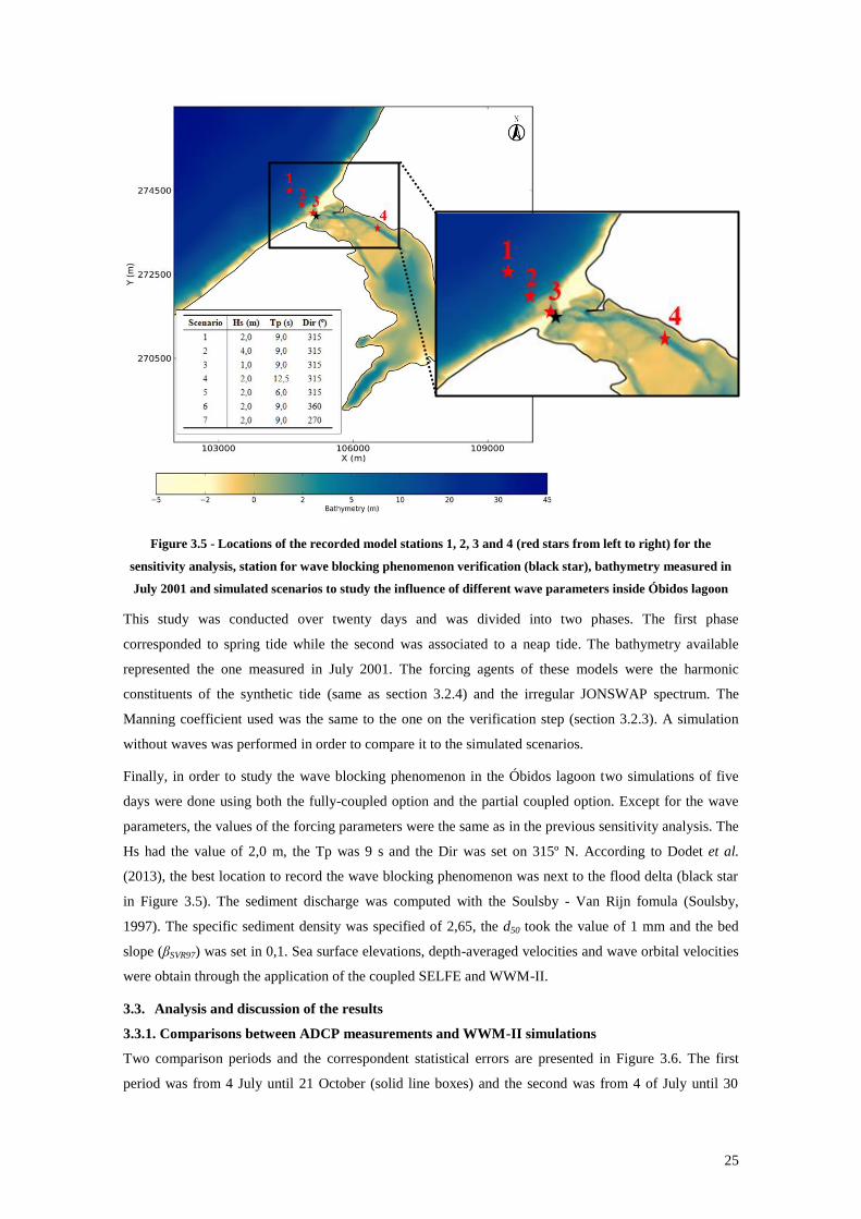
25
Figure 3.5 - Locations of the recorded model stations 1, 2, 3 and 4 (red stars from left to right) for the
sensitivity analysis, station for wave blocking phenomenon verification (black star), bathymetry measured in
July 2001 and simulated scenarios to study the influence of different wave parameters inside Óbidos lagoon
This study was conducted over twenty days and was divided into two phases. The first phase
corresponded to spring tide while the second was associated to a neap tide. The bathymetry available
represented the one measured in July 2001. The forcing agents of these models were the harmonic
constituents of the synthetic tide (same as section 3.2.4) and the irregular JONSWAP spectrum. The
Manning coefficient used was the same to the one on the verification step (section 3.2.3). A simulation
without waves was performed in order to compare it to the simulated scenarios.
Finally, in order to study the wave blocking phenomenon in the Óbidos lagoon two simulations of five
days were done using both the fully-coupled option and the partial coupled option. Except for the wave
parameters, the values of the forcing parameters were the same as in the previous sensitivity analysis. The
Hs had the value of 2,0 m, the Tp was 9 s and the Dir was set on 315º N. According to Dodet et al.
(2013), the best location to record the wave blocking phenomenon was next to the flood delta (black star
in Figure 3.5). The sediment discharge was computed with the Soulsby - Van Rijn fomula (Soulsby,
1997). The specific sediment density was specified of 2,65, the d50 took the value of 1 mm and the bed
slope (βSVR97) was set in 0,1. Sea surface elevations, depth-averaged velocities and wave orbital velocities
were obtain through the application of the coupled SELFE and WWM-II.
3.3. Analysis and discussion of the results
3.3.1. Comparisons between ADCP measurements and WWM-II simulations
Two comparison periods and the correspondent statistical errors are presented in Figure 3.6. The first
period was from 4 July until 21 October (solid line boxes) and the second was from 4 of July until 30
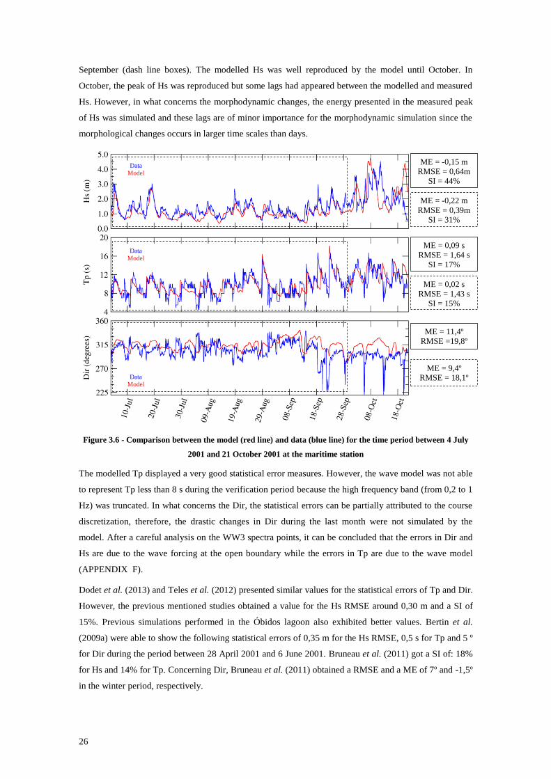
26
September (dash line boxes). The modelled Hs was well reproduced by the model until October. In
October, the peak of Hs was reproduced but some lags had appeared between the modelled and measured
Hs. However, in what concerns the morphodynamic changes, the energy presented in the measured peak
of Hs was simulated and these lags are of minor importance for the morphodynamic simulation since the
morphological changes occurs in larger time scales than days.
Figure 3.6 - Comparison between the model (red line) and data (blue line) for the time period between 4 July
2001 and 21 October 2001 at the maritime station
The modelled Tp displayed a very good statistical error measures. However, the wave model was not able
to represent Tp less than 8 s during the verification period because the high frequency band (from 0,2 to 1
Hz) was truncated. In what concerns the Dir, the statistical errors can be partially attributed to the course
discretization, therefore, the drastic changes in Dir during the last month were not simulated by the
model. After a careful analysis on the WW3 spectra points, it can be concluded that the errors in Dir and
Hs are due to the wave forcing at the open boundary while the errors in Tp are due to the wave model
(APPENDIX F).
Dodet et al. (2013) and Teles et al. (2012) presented similar values for the statistical errors of Tp and Dir.
However, the previous mentioned studies obtained a value for the Hs RMSE around 0,30 m and a SI of
15%. Previous simulations performed in the Óbidos lagoon also exhibited better values. Bertin et al.
(2009a) were able to show the following statistical errors of 0,35 m for the Hs RMSE, 0,5 s for Tp and 5 º
for Dir during the period between 28 April 2001 and 6 June 2001. Bruneau et al. (2011) got a SI of: 18%
for Hs and 14% for Tp. Concerning Dir, Bruneau et al. (2011) obtained a RMSE and a ME of 7º and -1,5º
in the winter period, respectively.
ME = 0,09 s
RMSE = 1,64 s
SI = 17%
ME = 11,4º
RMSE =19,8º
ME = -0,22 m
RMSE = 0,39m
SI = 31%
ME = 0,02 s
RMSE = 1,43 s
SI = 15%
ME = 9,4º
RMSE = 18,1º
ME = -0,15 m
RMSE = 0,64m
SI = 44%
Data
Model
Data
Model
Data
Model
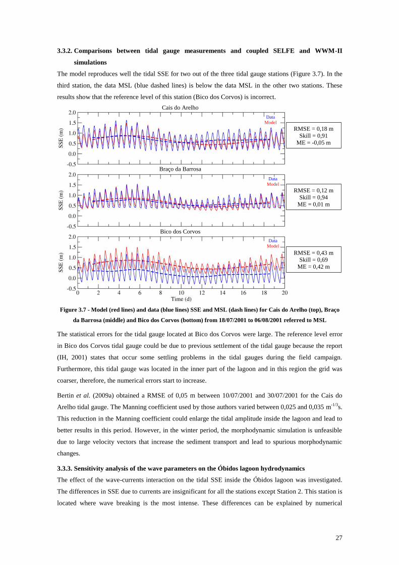
27
3.3.2. Comparisons between tidal gauge measurements and coupled SELFE and WWM-II
simulations
The model reproduces well the tidal SSE for two out of the three tidal gauge stations (Figure 3.7). In the
third station, the data MSL (blue dashed lines) is below the data MSL in the other two stations. These
results show that the reference level of this station (Bico dos Corvos) is incorrect.
Figure 3.7 - Model (red lines) and data (blue lines) SSE and MSL (dash lines) for Cais do Arelho (top), Braço
da Barrosa (middle) and Bico dos Corvos (bottom) from 18/07/2001 to 06/08/2001 referred to MSL
The statistical errors for the tidal gauge located at Bico dos Corvos were large. The reference level error
in Bico dos Corvos tidal gauge could be due to previous settlement of the tidal gauge because the report
(IH, 2001) states that occur some settling problems in the tidal gauges during the field campaign.
Furthermore, this tidal gauge was located in the inner part of the lagoon and in this region the grid was
coarser, therefore, the numerical errors start to increase.
Bertin et al. (2009a) obtained a RMSE of 0,05 m between 10/07/2001 and 30/07/2001 for the Cais do
Arelho tidal gauge. The Manning coefficient used by those authors varied between 0,025 and 0,035 m-1/3
s.
This reduction in the Manning coefficient could enlarge the tidal amplitude inside the lagoon and lead to
better results in this period. However, in the winter period, the morphodynamic simulation is unfeasible
due to large velocity vectors that increase the sediment transport and lead to spurious morphodynamic
changes.
3.3.3. Sensitivity analysis of the wave parameters on the Óbidos lagoon hydrodynamics
The effect of the wave-currents interaction on the tidal SSE inside the Óbidos lagoon was investigated.
The differences in SSE due to currents are insignificant for all the stations except Station 2. This station is
located where wave breaking is the most intense. These differences can be explained by numerical
RMSE = 0,18 m
Skill = 0,91
ME = -0,05 m
RMSE = 0,12 m
Skill = 0,94
ME = 0,01 m
RMSE = 0,43 m
Skill = 0,69
ME = 0,42 m
Cais do Arelho
Braço da Barrosa
Bico dos Corvos
Data
Model
Data
Model
Data
Model
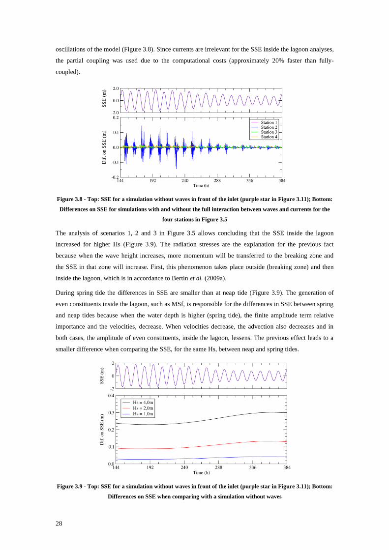
28
oscillations of the model (Figure 3.8). Since currents are irrelevant for the SSE inside the lagoon analyses,
the partial coupling was used due to the computational costs (approximately 20% faster than fully-
coupled).
Figure 3.8 - Top: SSE for a simulation without waves in front of the inlet (purple star in Figure 3.11); Bottom:
Differences on SSE for simulations with and without the full interaction between waves and currents for the
four stations in Figure 3.5
The analysis of scenarios 1, 2 and 3 in Figure 3.5 allows concluding that the SSE inside the lagoon
increased for higher Hs (Figure 3.9). The radiation stresses are the explanation for the previous fact
because when the wave height increases, more momentum will be transferred to the breaking zone and
the SSE in that zone will increase. First, this phenomenon takes place outside (breaking zone) and then
inside the lagoon, which is in accordance to Bertin et al. (2009a).
During spring tide the differences in SSE are smaller than at neap tide (Figure 3.9). The generation of
even constituents inside the lagoon, such as MSf, is responsible for the differences in SSE between spring
and neap tides because when the water depth is higher (spring tide), the finite amplitude term relative
importance and the velocities, decrease. When velocities decrease, the advection also decreases and in
both cases, the amplitude of even constituents, inside the lagoon, lessens. The previous effect leads to a
smaller difference when comparing the SSE, for the same Hs, between neap and spring tides.
Figure 3.9 - Top: SSE for a simulation without waves in front of the inlet (purple star in Figure 3.11); Bottom:
Differences on SSE when comparing with a simulation without waves
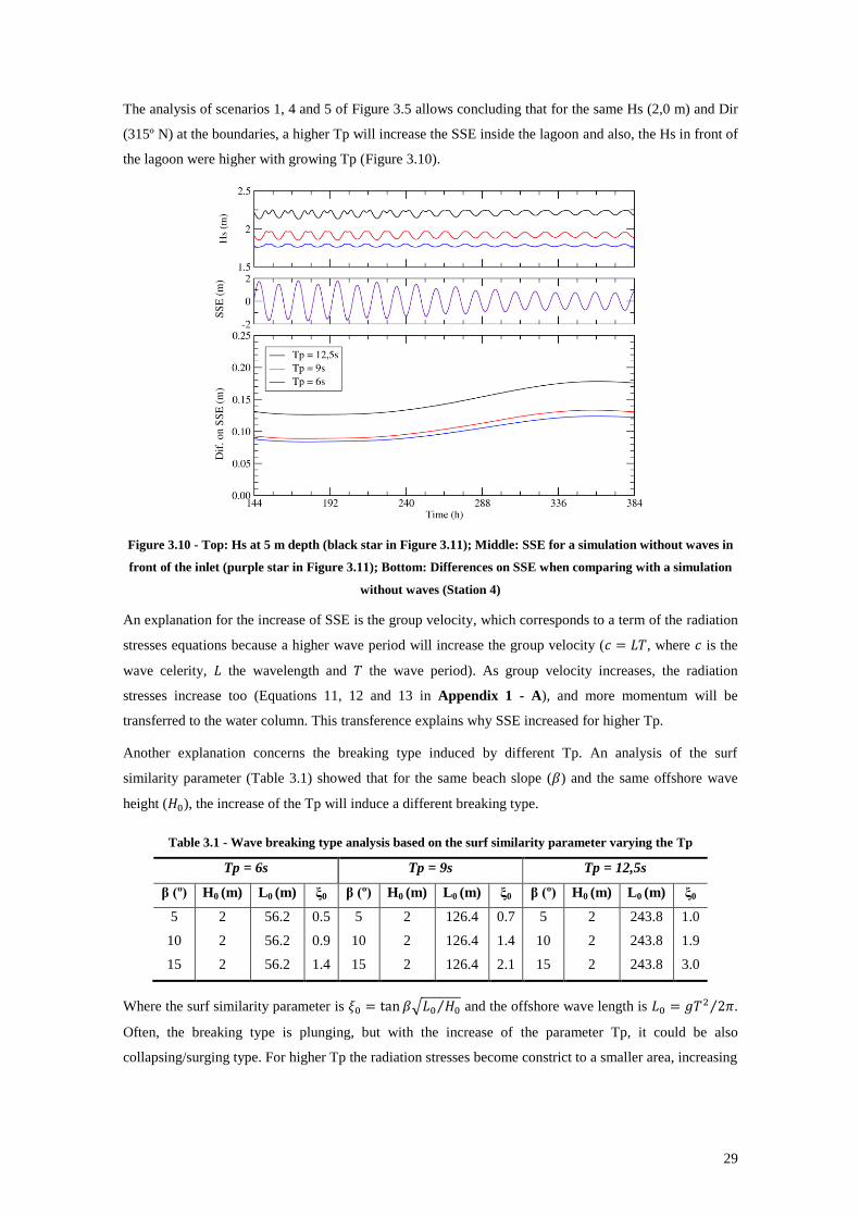
29
The analysis of scenarios 1, 4 and 5 of Figure 3.5 allows concluding that for the same Hs (2,0 m) and Dir
(315º N) at the boundaries, a higher Tp will increase the SSE inside the lagoon and also, the Hs in front of
the lagoon were higher with growing Tp (Figure 3.10).
Figure 3.10 - Top: Hs at 5 m depth (black star in Figure 3.11); Middle: SSE for a simulation without waves in
front of the inlet (purple star in Figure 3.11); Bottom: Differences on SSE when comparing with a simulation
without waves (Station 4)
An explanation for the increase of SSE is the group velocity, which corresponds to a term of the radiation
stresses equations because a higher wave period will increase the group velocity (𝑐 = 𝐿𝑇, where 𝑐 is the
wave celerity, 𝐿 the wavelength and 𝑇 the wave period). As group velocity increases, the radiation
stresses increase too (Equations 11, 12 and 13 in Appendix 1 - A), and more momentum will be
transferred to the water column. This transference explains why SSE increased for higher Tp.
Another explanation concerns the breaking type induced by different Tp. An analysis of the surf
similarity parameter (Table 3.1) showed that for the same beach slope (𝛽) and the same offshore wave
height (𝐻0), the increase of the Tp will induce a different breaking type.
Table 3.1 - Wave breaking type analysis based on the surf similarity parameter varying the Tp
Tp = 6s Tp = 9s Tp = 12,5s
β (º) H0 (m) L0 (m) ξ0 β (º) H0 (m) L0 (m) ξ0 β (º) H0 (m) L0 (m) ξ0
5 2 56.2 0.5 5 2 126.4 0.7 5 2 243.8 1.0
10 2 56.2 0.9 10 2 126.4 1.4 10 2 243.8 1.9
15 2 56.2 1.4 15 2 126.4 2.1 15 2 243.8 3.0
Where the surf similarity parameter is 𝜉0 = tan 𝛽√𝐿0 𝐻0⁄ and the offshore wave length is 𝐿0 = 𝑔𝑇2 2𝜋⁄ .
Often, the breaking type is plunging, but with the increase of the parameter Tp, it could be also
collapsing/surging type. For higher Tp the radiation stresses become constrict to a smaller area, increasing
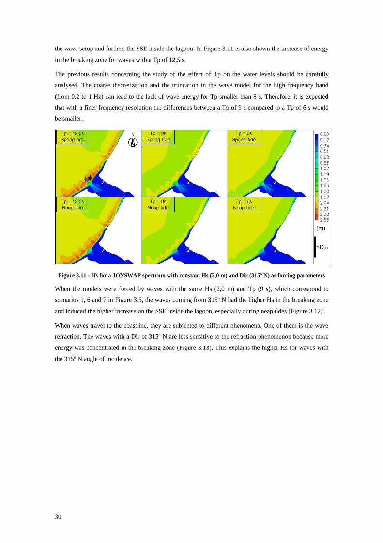
30
the wave setup and further, the SSE inside the lagoon. In Figure 3.11 is also shown the increase of energy
in the breaking zone for waves with a Tp of 12,5 s.
The previous results concerning the study of the effect of Tp on the water levels should be carefully
analysed. The coarse discretization and the truncation in the wave model for the high frequency band
(from 0,2 to 1 Hz) can lead to the lack of wave energy for Tp smaller than 8 s. Therefore, it is expected
that with a finer frequency resolution the differences between a Tp of 9 s compared to a Tp of 6 s would
be smaller.
Figure 3.11 - Hs for a JONSWAP spectrum with constant Hs (2,0 m) and Dir (315º N) as forcing parameters
When the models were forced by waves with the same Hs (2,0 m) and Tp (9 s), which correspond to
scenarios 1, 6 and 7 in Figure 3.5, the waves coming from 315º N had the higher Hs in the breaking zone
and induced the higher increase on the SSE inside the lagoon, especially during neap tides (Figure 3.12).
When waves travel to the coastline, they are subjected to different phenomena. One of them is the wave
refraction. The waves with a Dir of 315º N are less sensitive to the refraction phenomenon because more
energy was concentrated in the breaking zone (Figure 3.13). This explains the higher Hs for waves with
the 315º N angle of incidence.
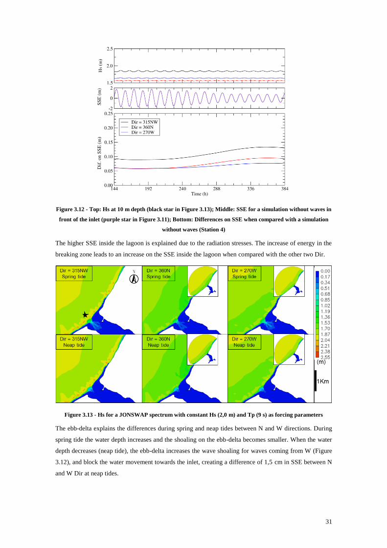
31
Figure 3.12 - Top: Hs at 10 m depth (black star in Figure 3.13); Middle: SSE for a simulation without waves in
front of the inlet (purple star in Figure 3.11); Bottom: Differences on SSE when compared with a simulation
without waves (Station 4)
The higher SSE inside the lagoon is explained due to the radiation stresses. The increase of energy in the
breaking zone leads to an increase on the SSE inside the lagoon when compared with the other two Dir.
Figure 3.13 - Hs for a JONSWAP spectrum with constant Hs (2,0 m) and Tp (9 s) as forcing parameters
The ebb-delta explains the differences during spring and neap tides between N and W directions. During
spring tide the water depth increases and the shoaling on the ebb-delta becomes smaller. When the water
depth decreases (neap tide), the ebb-delta increases the wave shoaling for waves coming from W (Figure
3.12), and block the water movement towards the inlet, creating a difference of 1,5 cm in SSE between N
and W Dir at neap tides.
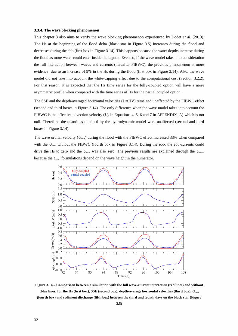
32
3.3.4. The wave blocking phenomenon
This chapter 3 also aims to verify the wave blocking phenomenon experienced by Dodet et al. (2013).
The Hs at the beginning of the flood delta (black star in Figure 3.5) increases during the flood and
decreases during the ebb (first box in Figure 3.14). This happens because the water depths increase during
the flood as more water could enter inside the lagoon. Even so, if the wave model takes into consideration
the full interaction between waves and currents (hereafter FIBWC), the previous phenomenon is more
evidence due to an increase of 9% in the Hs during the flood (first box in Figure 3.14). Also, the wave
model did not take into account the white-capping effect due to the computational cost (Section 3.2.2).
For that reason, it is expected that the Hs time series for the fully-coupled option will have a more
asymmetric profile when compared with the time series of Hs for the partial coupled option.
The SSE and the depth-averaged horizontal velocities (DAHV) remained unaffected by the FIBWC effect
(second and third boxes in Figure 3.14). The only difference when the wave model takes into account the
FIBWC is the effective advection velocity (UA in Equations 4, 5, 6 and 7 in APPENDIX A) which is not
null. Therefore, the quantities obtained by the hydrodynamic model were unaffected (second and third
boxes in Figure 3.14).
The wave orbital velocity (Urms) during the flood with the FIBWC effect increased 33% when compared
with the Urms without the FIBWC (fourth box in Figure 3.14). During the ebb, the ebb-currents could
drive the Hs to zero and the Urms was also zero. The previous results are explained through the Urms,
because the Urms formulations depend on the wave height in the numerator.
Figure 3.14 – Comparison between a simulation with the full wave-current interaction (red lines) and without
(blue lines) for the Hs (first box), SSE (second box), depth-average horizontal velocities (third box), Urms
(fourth box) and sediment discharge (fifth box) between the third and fourth days on the black star (Figure
3.5)
Urm
s (m
/s)
fully-coupled
partial coupled

33
The sediment transport was computed with the Soulby – Van Rijn (Soulsby, 1997) formula. The results
show that with the FIBWC effect, the sediment transport increased by 30% during the flood (fifth box in
Figure 3.14). The Urms explains the previous fact because, with the FIBWC effect, waves will put more
sediment in suspension and then, the flood currents will transport them towards the lagoon. This way, the
net sediment transport towards the lagoon increased over a tidal cycle, which is in accordance to the study
made by Dodet et al. (2013).

35
4. Assessment of three dredging plans for the Óbidos lagoon
SUMMARY: This chapter concerns the assessment of three dredging plans to evaluate the improvements
regarding the Óbidos lagoon inlet stability. A morphodynamic model which simulates the non-cohesive
sediment transport taking into account the wave-current interaction was used to assess the morphological
evolution during five months of three dredging plans. The results of the following simulations are
reported: tidal prism, differences between ebb and flood durations, sediment volumes and fluxes through
the inlet and application of empirical stability relationships to the Óbidos lagoon inlet. From these results,
it is reasonable to assume that the new dredging plans improved the hydrodynamic conditions of the
Óbidos lagoon. Morphologically, the higher dredging depths of the new dredging plans promoted the
sediment accretion at the flood-delta. The addition of transverse channels improved the sediment export
capacity during the studied period. This chapter ends with a summary which discusses the main
advantages and drawbacks of each studied dredging plan in the Óbidos lagoon.
4.1. Review on seasonal closure, tidal distortions and dredging solutions in wave-dominated inlets
Understanding the dominant processes that control the morphodynamic changes in inlets is a key issue to
develop sustainable engineering solutions. Ranasinghe and Pattiaratchi (2003) successfully pioneered in
the simulation of the closure of a tidal inlet. They presented two mechanisms that are required in a
morphodynamic model:
1) the interaction between inlet current and longshore currents
2) the effect of both inlet current and onshore sediment transport.
The first mechanism is described as the interruption of the longshore current by the inlet. As a
consequence, this interaction will also interrupt the longshore sediment transport and induce the
formation of a shoal up-drift of the inlet. The intensity of the longshore sediment transport will control the
growth and the size of this shoal. If the inlet current (ebb-current) is strong enough to erode the sediments
previously deposited, then the spit will not migrate downdrift. However, if the inlet current cannot erode
the sediments in this shoal, a spit will continue to grow until the inlet closes or migrates.
The second mechanism can only dominate if the inlet current is small (less than 1 m/s) and in micro-tidal
regimes. In such conditions, the tidal prism will be small. In the winter and under storm conditions, a
linear bar is formed across the breaker zone. After the storm, the presence of long-period swell waves will
continue to move the sand stored in the linear bar onshore. When the ebb currents are weak, the onshore
sand transport, previously accumulated in the linear bar, will induce the inlet closure.
Bertin et al. (2015) have mainly focused their study on wave-related processes, which are the most
important on wave-dominated inlets. They presented and verified the “bulldozer effect” studied in detail
by Suastika (2004). Another wave-related process presented by Bertin et al. (2015) is the presence of
lateral barotropic pressure gradients which accelerate the longshore flows towards the inlet.
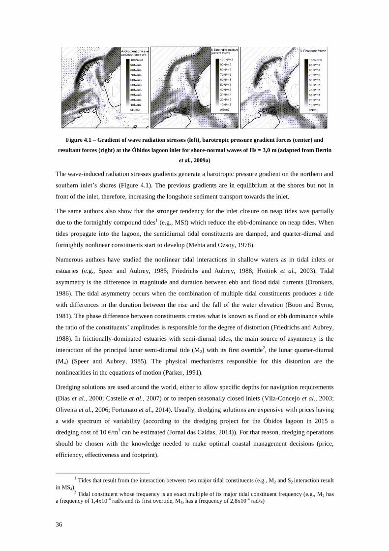
36
Figure 4.1 – Gradient of wave radiation stresses (left), barotropic pressure gradient forces (center) and
resultant forces (right) at the Óbidos lagoon inlet for shore-normal waves of Hs = 3,0 m (adapted from Bertin
et al., 2009a)
The wave-induced radiation stresses gradients generate a barotropic pressure gradient on the northern and
southern inlet’s shores (Figure 4.1). The previous gradients are in equilibrium at the shores but not in
front of the inlet, therefore, increasing the longshore sediment transport towards the inlet.
The same authors also show that the stronger tendency for the inlet closure on neap tides was partially
due to the fortnightly compound tides1 (e.g., MSf) which reduce the ebb-dominance on neap tides. When
tides propagate into the lagoon, the semidiurnal tidal constituents are damped, and quarter-diurnal and
fortnightly nonlinear constituents start to develop (Mehta and Ozsoy, 1978).
Numerous authors have studied the nonlinear tidal interactions in shallow waters as in tidal inlets or
estuaries (e.g., Speer and Aubrey, 1985; Friedrichs and Aubrey, 1988; Hoitink et al., 2003). Tidal
asymmetry is the difference in magnitude and duration between ebb and flood tidal currents (Dronkers,
1986). The tidal asymmetry occurs when the combination of multiple tidal constituents produces a tide
with differences in the duration between the rise and the fall of the water elevation (Boon and Byrne,
1981). The phase difference between constituents creates what is known as flood or ebb dominance while
the ratio of the constituents’ amplitudes is responsible for the degree of distortion (Friedrichs and Aubrey,
1988). In frictionally-dominated estuaries with semi-diurnal tides, the main source of asymmetry is the
interaction of the principal lunar semi-diurnal tide (M2) with its first overtide2, the lunar quarter-diurnal
(M4) (Speer and Aubrey, 1985). The physical mechanisms responsible for this distortion are the
nonlinearities in the equations of motion (Parker, 1991).
Dredging solutions are used around the world, either to allow specific depths for navigation requirements
(Dias et al., 2000; Castelle et al., 2007) or to reopen seasonally closed inlets (Vila-Concejo et al., 2003;
Oliveira et al., 2006; Fortunato et al., 2014). Usually, dredging solutions are expensive with prices having
a wide spectrum of variability (according to the dredging project for the Óbidos lagoon in 2015 a
dredging cost of 10 €/m3 can be estimated (Jornal das Caldas, 2014)). For that reason, dredging operations
should be chosen with the knowledge needed to make optimal coastal management decisions (price,
efficiency, effectiveness and footprint).
1 Tides that result from the interaction between two major tidal constituents (e.g., M2 and S2 interaction result
in MS4). 2 Tidal constituent whose frequency is an exact multiple of its major tidal constituent frequency (e.g., M2 has
a frequency of 1,4x10⁻⁴ rad/s and its first overtide, M4, has a frequency of 2,8x10⁻⁴ rad/s)
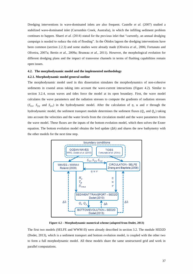
37
Dredging interventions in wave-dominated inlets are also frequent. Castelle et al. (2007) studied a
stabilized wave-dominated inlet (Currumbin Creek, Australia), in which the infilling sediment problem
continues to happen. Shaeri et al. (2014) stated for the previous inlet that “currently, an annual dredging
campaign is needed to reduce the risk of flooding”. In the Óbidos lagoon the dredging interventions have
been common (section 2.2.3) and some studies were already made (Oliveira et al., 2006; Fortunato and
Oliveira, 2007a; Bertin et al., 2009a; Bruneau et al., 2011). However, the morphological evolution for
different dredging plans and the impact of transverse channels in terms of flushing capabilities remain
open issues.
4.2. The morphodynamic model and the implemented methodology
4.2.1. Morphodynamic model general outline
The morphodynamic model used in this dissertation simulates the morphodynamics of non-cohesive
sediments in coastal areas taking into account the wave-current interactions (Figure 4.2). Similar to
section 3.2.4, ocean waves and tides force the model at its open boundary. First, the wave model
calculates the wave parameters and the radiation stresses to compute the gradients of radiation stresses
(𝑆𝑥𝑥, 𝑆𝑦𝑦 and 𝑆𝑦𝑥) in the hydrodynamic model. After the calculation of 𝜂, 𝑢 and 𝑣 through the
hydrodynamic model, the sediment transport module determines the sediment fluxes (𝑄𝑥 and 𝑄𝑦) taking
into account the velocities and the water levels from the circulation model and the wave parameters from
the wave model. These fluxes are the inputs of the bottom evolution model, which then solves the Exner
equation. The bottom evolution model obtains the bed update (∆ℎ) and shares the new bathymetry with
the other models for the next time step.
Figure 4.2 – Morphodynamic numerical scheme (adapted from Dodet, 2013)
The first two models (SELFE and WWM-II) were already described in section 3.2. The module SED2D
(Dodet, 2013), which is a sediment transport and bottom evolution model, is coupled with the other two
to form a full morphodynamic model. All these models share the same unstructured grid and work in
parallel computations.
38
4.2.2. The sediment transport and bottom evolution model – SED2D
The sediment transport model has several alternative sediment transport formulations, ranging from the
traditional ones (e.g., Eugelund and Hansen, 1967; Ackers and White, 1973) to the most recent, which
include the sediment transport induced by waves (e.g., Camenon and Larsson, 2005 and 2008). In this
dissertation, the Van Rijn (2007a,b) sediment transport formulation was used. This formulation takes into
account both the bedload and the suspension transport, and is applicable to a wide spectrum of particle
sizes (between 0,05 mm to 2 mm). Also, it includes the effects of both waves and currents. Usually,
sediment transport formulations are derived for flat bottom conditions. To overcome this limitation,
Lesser et al. (2004) proposed a formulation to include the bed-slope effect and SED2D takes this effect
into consideration.
SED2D solves the Exner equation through a node-centred finite volume technique to update the bottom
bathymetry every 20 s. In this dissertation, three filters were used due to the oscillations inherent to
morphodynamic models:
1) an extrema filter
2) a slope filter
3) a diffusive filter.
Fortunato and Oliveira (2000) implemented the extrema filter to eliminate local extremes in the
bathymetry after each morphodynamic time step. This filter is volume-conservative and introduces small
numerical diffusion (Oliveira and Fortunato, 2002).
Avalanching was taken into account using a slope filter. After each morphodynamic time step, this filter
limits the local slopes to a user-specified threshold. Roelvink et al. (2009) studied a beach profile and
defined these values as 1 for dry and 0,3 for wet areas. Dodet (2013) used 1 for dry and 0,2 for wet areas
in the Albufeira lagoon, despite the fact that this author was able to stabilize the sediment model without
using this filter. In this dissertation, the slope filter took the value of 1 for dry and 0,2 for wet areas.
The diffusion filter (Fortunato and Oliveira, 2007b) aims to prevent the development of spatial
oscillations through a modification on the Exner equation (Equation 26 in APPENDIX A). The value of
the coefficient 𝜀 was set to 2, which is in accordance with Fortunato et al. (2014). All the details
regarding the equations solved by SED2D are in APPENDIX A.
To summarize, the sediment fluxes (𝑄𝑥 and 𝑄𝑦) are calculated with one of the available formulations
(Van Rijn, 2007a,b) taking into account the bed-slope effect (Lesser et al., 2004) and the modified
sediment fluxes (Fortunato and Oliveira, 2007b). Then, the calculation of the Exner equation with a node-
centred method is used to update the bottom bathymetry. Before computing the next time step, the local
extremes in the bathymetry were smoothed with the extrema filter (Fortunato and Oliveira, 2000) and the
slope filter ensures that all element slopes are lower than a defined threshold. Finally, the model shares
the bottom update (∆ℎ) with the wave and the hydrodynamic model and proceeds to the next time step.
The sediment median grain diameter (𝑑50) was specified on SED2D (d50.gr3) and was adapted from
Bruneau et al. (2011). Due to numerical oscillations on the northern and southern coasts, the 𝑑50 needs to
be increased by approximately 0,4 mm in order to prevent oscillations (Figure 4.3). Previous simulations
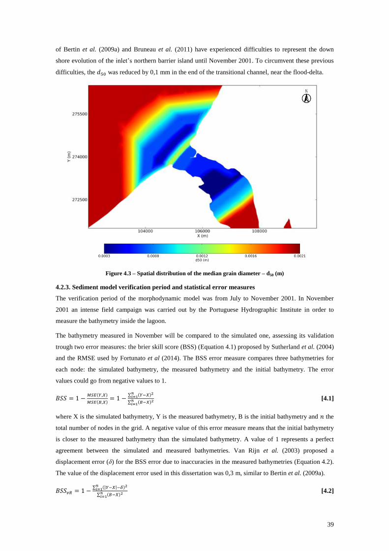
39
of Bertin et al. (2009a) and Bruneau et al. (2011) have experienced difficulties to represent the down
shore evolution of the inlet’s northern barrier island until November 2001. To circumvent these previous
difficulties, the 𝑑50 was reduced by 0,1 mm in the end of the transitional channel, near the flood-delta.
Figure 4.3 – Spatial distribution of the median grain diameter – d50 (m)
4.2.3. Sediment model verification period and statistical error measures
The verification period of the morphodynamic model was from July to November 2001. In November
2001 an intense field campaign was carried out by the Portuguese Hydrographic Institute in order to
measure the bathymetry inside the lagoon.
The bathymetry measured in November will be compared to the simulated one, assessing its validation
trough two error measures: the brier skill score (BSS) (Equation 4.1) proposed by Sutherland et al. (2004)
and the RMSE used by Fortunato et al (2014). The BSS error measure compares three bathymetries for
each node: the simulated bathymetry, the measured bathymetry and the initial bathymetry. The error
values could go from negative values to 1.
𝐵𝑆𝑆 = 1 −𝑀𝑆𝐸(𝑌,𝑋)
𝑀𝑆𝐸(𝐵,𝑋)= 1 −
∑ (𝑌−𝑋)2𝑛𝑖=1
∑ (𝐵−𝑋)2𝑛𝑖=1
[4.1]
where X is the simulated bathymetry, Y is the measured bathymetry, B is the initial bathymetry and 𝑛 the
total number of nodes in the grid. A negative value of this error measure means that the initial bathymetry
is closer to the measured bathymetry than the simulated bathymetry. A value of 1 represents a perfect
agreement between the simulated and measured bathymetries. Van Rijn et al. (2003) proposed a
displacement error (δ) for the BSS error due to inaccuracies in the measured bathymetries (Equation 4.2).
The value of the displacement error used in this dissertation was 0,3 m, similar to Bertin et al. (2009a).
𝐵𝑆𝑆𝑣𝑅 = 1 −∑ (|𝑌−𝑋|−𝛿)2𝑛
𝑖=1
∑ (𝐵−𝑋)2𝑛𝑖=1
[4.2]
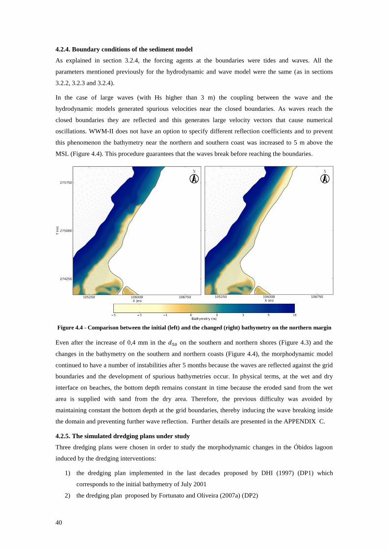
40
4.2.4. Boundary conditions of the sediment model
As explained in section 3.2.4, the forcing agents at the boundaries were tides and waves. All the
parameters mentioned previously for the hydrodynamic and wave model were the same (as in sections
3.2.2, 3.2.3 and 3.2.4).
In the case of large waves (with Hs higher than 3 m) the coupling between the wave and the
hydrodynamic models generated spurious velocities near the closed boundaries. As waves reach the
closed boundaries they are reflected and this generates large velocity vectors that cause numerical
oscillations. WWM-II does not have an option to specify different reflection coefficients and to prevent
this phenomenon the bathymetry near the northern and southern coast was increased to 5 m above the
MSL (Figure 4.4). This procedure guarantees that the waves break before reaching the boundaries.
Even after the increase of 0,4 mm in the 𝑑50 on the southern and northern shores (Figure 4.3) and the
changes in the bathymetry on the southern and northern coasts (Figure 4.4), the morphodynamic model
continued to have a number of instabilities after 5 months because the waves are reflected against the grid
boundaries and the development of spurious bathymetries occur. In physical terms, at the wet and dry
interface on beaches, the bottom depth remains constant in time because the eroded sand from the wet
area is supplied with sand from the dry area. Therefore, the previous difficulty was avoided by
maintaining constant the bottom depth at the grid boundaries, thereby inducing the wave breaking inside
the domain and preventing further wave reflection. Further details are presented in the APPENDIX C.
4.2.5. The simulated dredging plans under study
Three dredging plans were chosen in order to study the morphodynamic changes in the Óbidos lagoon
induced by the dredging interventions:
1) the dredging plan implemented in the last decades proposed by DHI (1997) (DP1) which
corresponds to the initial bathymetry of July 2001
2) the dredging plan proposed by Fortunato and Oliveira (2007a) (DP2)
Figure 4.4 - Comparison between the initial (left) and the changed (right) bathymetry on the northern margin
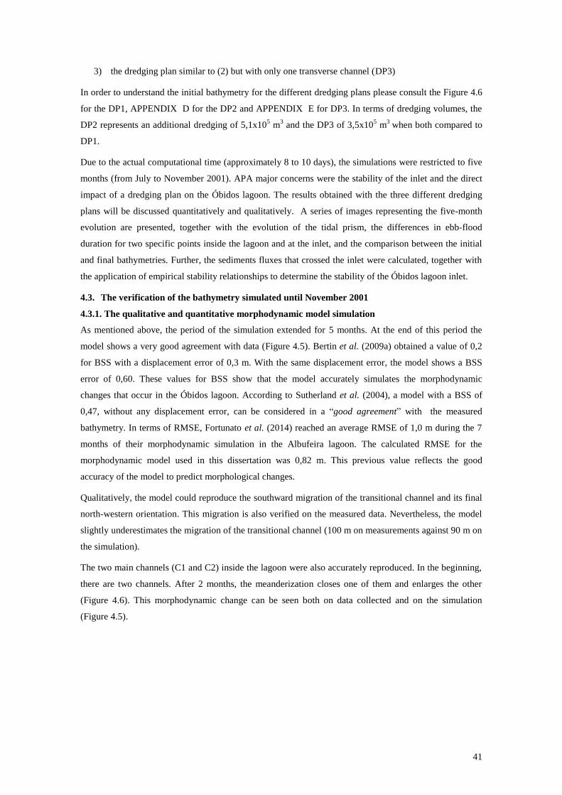
41
3) the dredging plan similar to (2) but with only one transverse channel (DP3)
In order to understand the initial bathymetry for the different dredging plans please consult the Figure 4.6
for the DP1, APPENDIX D for the DP2 and APPENDIX E for DP3. In terms of dredging volumes, the
DP2 represents an additional dredging of 5,1x10⁵ m
3 and the DP3 of 3,5x10
5 m
3 when both compared to
DP1.
Due to the actual computational time (approximately 8 to 10 days), the simulations were restricted to five
months (from July to November 2001). APA major concerns were the stability of the inlet and the direct
impact of a dredging plan on the Óbidos lagoon. The results obtained with the three different dredging
plans will be discussed quantitatively and qualitatively. A series of images representing the five-month
evolution are presented, together with the evolution of the tidal prism, the differences in ebb-flood
duration for two specific points inside the lagoon and at the inlet, and the comparison between the initial
and final bathymetries. Further, the sediments fluxes that crossed the inlet were calculated, together with
the application of empirical stability relationships to determine the stability of the Óbidos lagoon inlet.
4.3. The verification of the bathymetry simulated until November 2001
4.3.1. The qualitative and quantitative morphodynamic model simulation
As mentioned above, the period of the simulation extended for 5 months. At the end of this period the
model shows a very good agreement with data (Figure 4.5). Bertin et al. (2009a) obtained a value of 0,2
for BSS with a displacement error of 0,3 m. With the same displacement error, the model shows a BSS
error of 0,60. These values for BSS show that the model accurately simulates the morphodynamic
changes that occur in the Óbidos lagoon. According to Sutherland et al. (2004), a model with a BSS of
0,47, without any displacement error, can be considered in a “good agreement” with the measured
bathymetry. In terms of RMSE, Fortunato et al. (2014) reached an average RMSE of 1,0 m during the 7
months of their morphodynamic simulation in the Albufeira lagoon. The calculated RMSE for the
morphodynamic model used in this dissertation was 0,82 m. This previous value reflects the good
accuracy of the model to predict morphological changes.
Qualitatively, the model could reproduce the southward migration of the transitional channel and its final
north-western orientation. This migration is also verified on the measured data. Nevertheless, the model
slightly underestimates the migration of the transitional channel (100 m on measurements against 90 m on
the simulation).
The two main channels (C1 and C2) inside the lagoon were also accurately reproduced. In the beginning,
there are two channels. After 2 months, the meanderization closes one of them and enlarges the other
(Figure 4.6). This morphodynamic change can be seen both on data collected and on the simulation
(Figure 4.5).
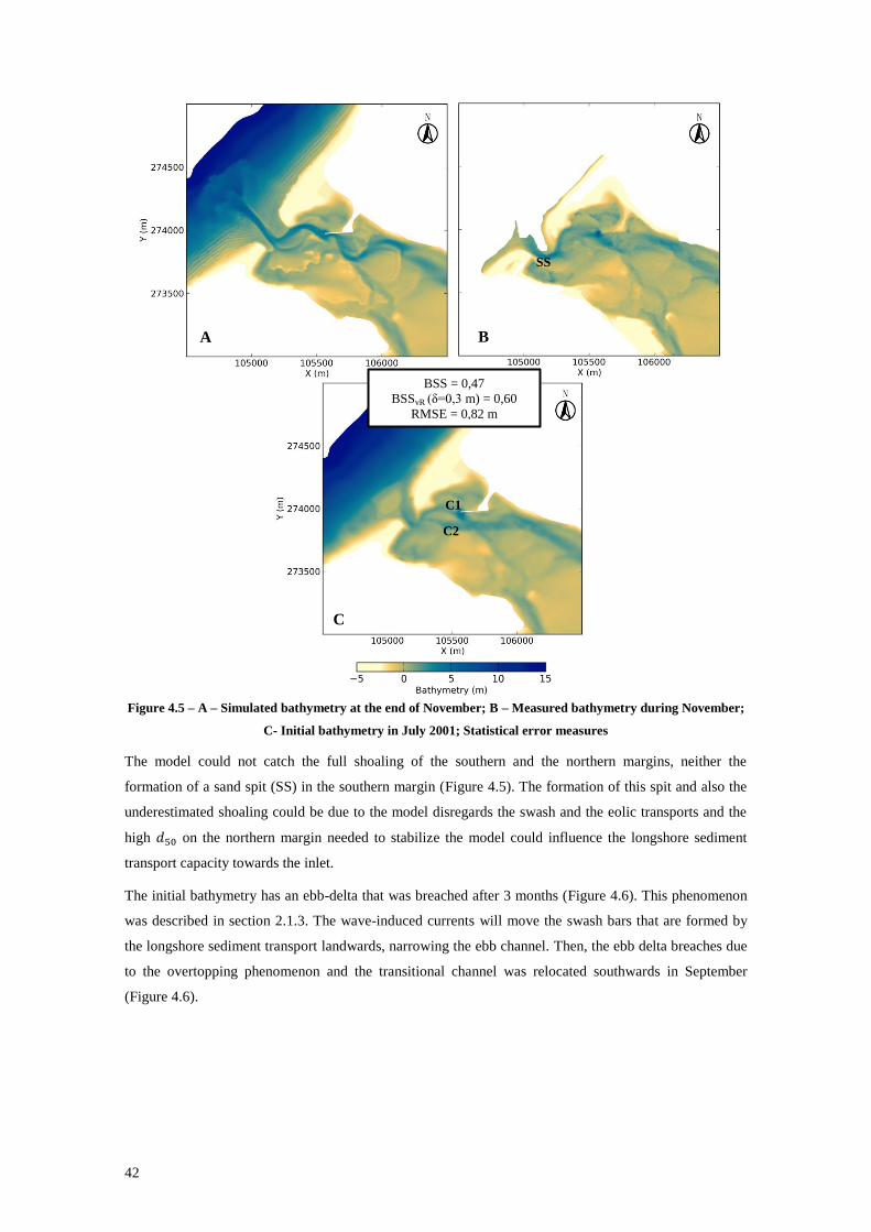
42
The model could not catch the full shoaling of the southern and the northern margins, neither the
formation of a sand spit (SS) in the southern margin (Figure 4.5). The formation of this spit and also the
underestimated shoaling could be due to the model disregards the swash and the eolic transports and the
high 𝑑50 on the northern margin needed to stabilize the model could influence the longshore sediment
transport capacity towards the inlet.
The initial bathymetry has an ebb-delta that was breached after 3 months (Figure 4.6). This phenomenon
was described in section 2.1.3. The wave-induced currents will move the swash bars that are formed by
the longshore sediment transport landwards, narrowing the ebb channel. Then, the ebb delta breaches due
to the overtopping phenomenon and the transitional channel was relocated southwards in September
(Figure 4.6).
A B
C
BSS = 0,47
BSSvR (δ=0,3 m) = 0,60
RMSE = 0,82 m
Figure 4.5 – A – Simulated bathymetry at the end of November; B – Measured bathymetry during November;
C- Initial bathymetry in July 2001; Statistical error measures
C1
C2
SS
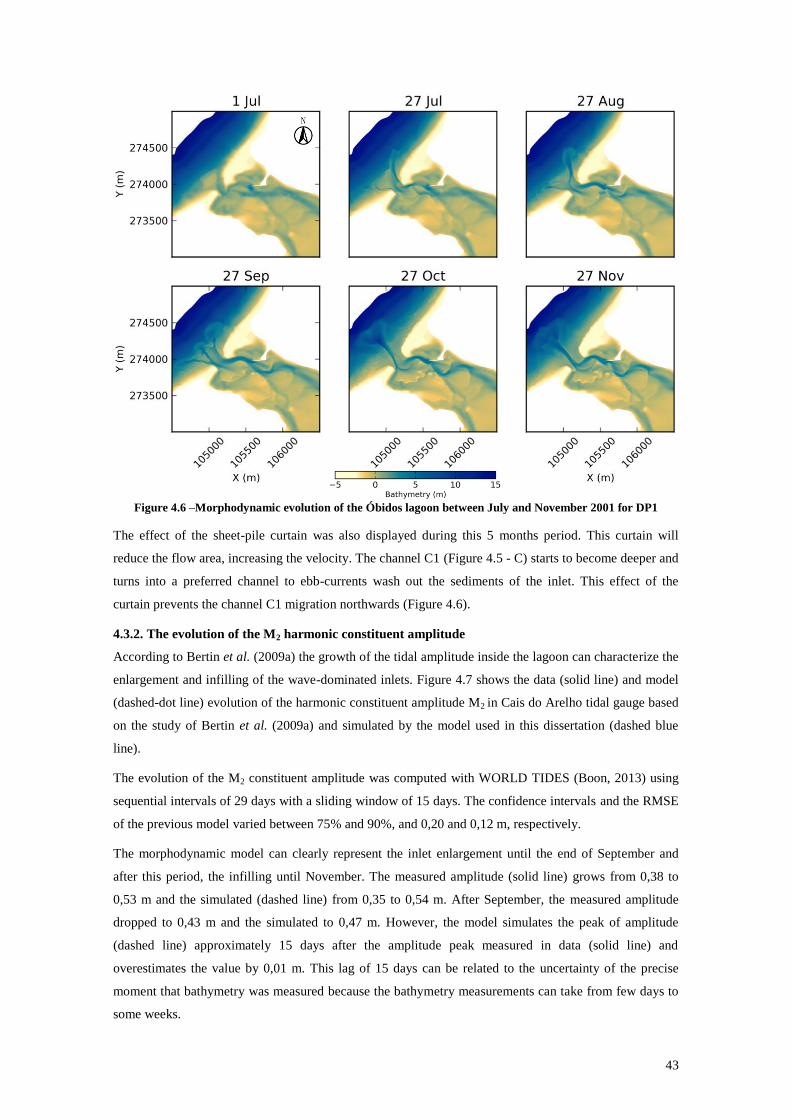
43
Figure 4.6 –Morphodynamic evolution of the Óbidos lagoon between July and November 2001 for DP1
The effect of the sheet-pile curtain was also displayed during this 5 months period. This curtain will
reduce the flow area, increasing the velocity. The channel C1 (Figure 4.5 - C) starts to become deeper and
turns into a preferred channel to ebb-currents wash out the sediments of the inlet. This effect of the
curtain prevents the channel C1 migration northwards (Figure 4.6).
4.3.2. The evolution of the M2 harmonic constituent amplitude
According to Bertin et al. (2009a) the growth of the tidal amplitude inside the lagoon can characterize the
enlargement and infilling of the wave-dominated inlets. Figure 4.7 shows the data (solid line) and model
(dashed-dot line) evolution of the harmonic constituent amplitude M2 in Cais do Arelho tidal gauge based
on the study of Bertin et al. (2009a) and simulated by the model used in this dissertation (dashed blue
line).
The evolution of the M2 constituent amplitude was computed with WORLD TIDES (Boon, 2013) using
sequential intervals of 29 days with a sliding window of 15 days. The confidence intervals and the RMSE
of the previous model varied between 75% and 90%, and 0,20 and 0,12 m, respectively.
The morphodynamic model can clearly represent the inlet enlargement until the end of September and
after this period, the infilling until November. The measured amplitude (solid line) grows from 0,38 to
0,53 m and the simulated (dashed line) from 0,35 to 0,54 m. After September, the measured amplitude
dropped to 0,43 m and the simulated to 0,47 m. However, the model simulates the peak of amplitude
(dashed line) approximately 15 days after the amplitude peak measured in data (solid line) and
overestimates the value by 0,01 m. This lag of 15 days can be related to the uncertainty of the precise
moment that bathymetry was measured because the bathymetry measurements can take from few days to
some weeks.
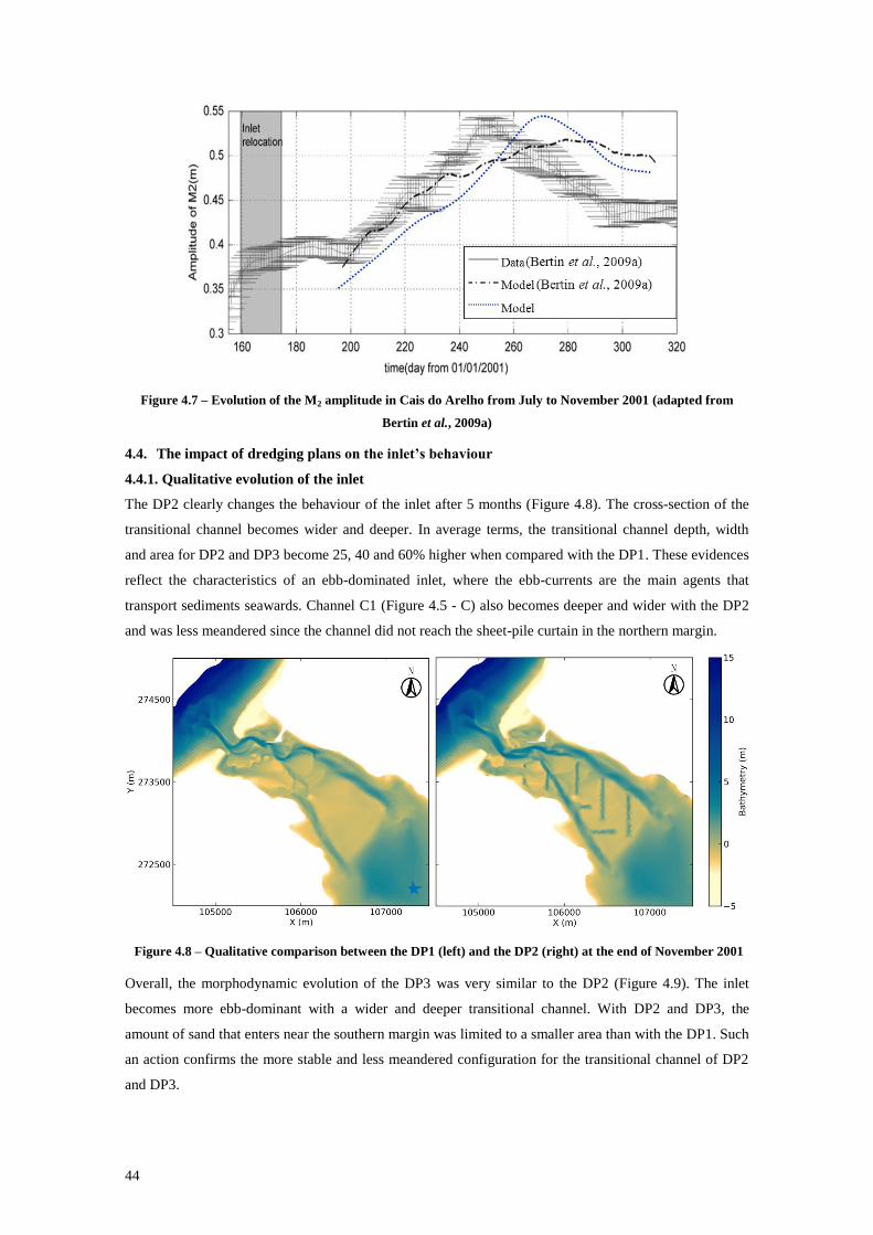
44
Figure 4.7 – Evolution of the M2 amplitude in Cais do Arelho from July to November 2001 (adapted from
Bertin et al., 2009a)
4.4. The impact of dredging plans on the inlet’s behaviour
4.4.1. Qualitative evolution of the inlet
The DP2 clearly changes the behaviour of the inlet after 5 months (Figure 4.8). The cross-section of the
transitional channel becomes wider and deeper. In average terms, the transitional channel depth, width
and area for DP2 and DP3 become 25, 40 and 60% higher when compared with the DP1. These evidences
reflect the characteristics of an ebb-dominated inlet, where the ebb-currents are the main agents that
transport sediments seawards. Channel C1 (Figure 4.5 - C) also becomes deeper and wider with the DP2
and was less meandered since the channel did not reach the sheet-pile curtain in the northern margin.
Overall, the morphodynamic evolution of the DP3 was very similar to the DP2 (Figure 4.9). The inlet
becomes more ebb-dominant with a wider and deeper transitional channel. With DP2 and DP3, the
amount of sand that enters near the southern margin was limited to a smaller area than with the DP1. Such
an action confirms the more stable and less meandered configuration for the transitional channel of DP2
and DP3.
Figure 4.8 – Qualitative comparison between the DP1 (left) and the DP2 (right) at the end of November 2001
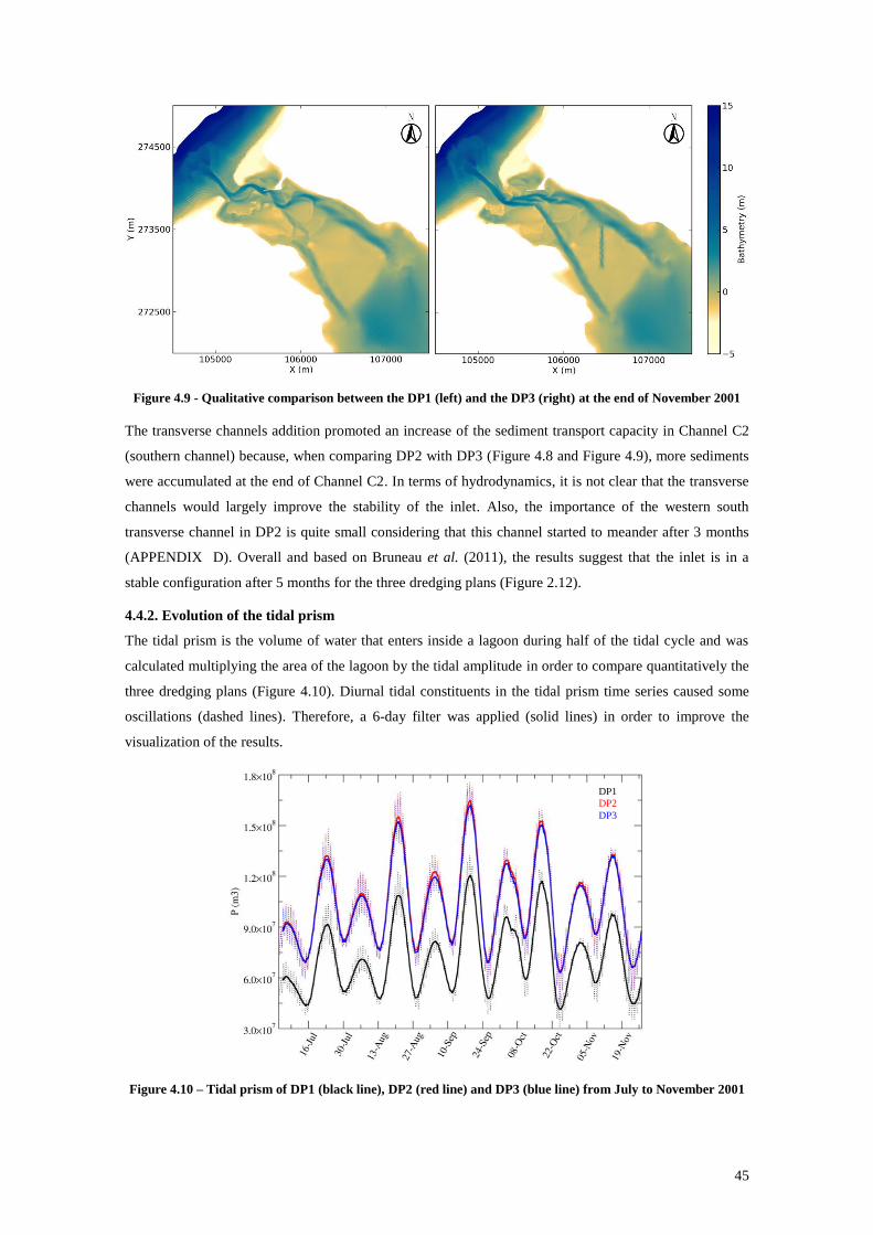
45
The transverse channels addition promoted an increase of the sediment transport capacity in Channel C2
(southern channel) because, when comparing DP2 with DP3 (Figure 4.8 and Figure 4.9), more sediments
were accumulated at the end of Channel C2. In terms of hydrodynamics, it is not clear that the transverse
channels would largely improve the stability of the inlet. Also, the importance of the western south
transverse channel in DP2 is quite small considering that this channel started to meander after 3 months
(APPENDIX D). Overall and based on Bruneau et al. (2011), the results suggest that the inlet is in a
stable configuration after 5 months for the three dredging plans (Figure 2.12).
4.4.2. Evolution of the tidal prism
The tidal prism is the volume of water that enters inside a lagoon during half of the tidal cycle and was
calculated multiplying the area of the lagoon by the tidal amplitude in order to compare quantitatively the
three dredging plans (Figure 4.10). Diurnal tidal constituents in the tidal prism time series caused some
oscillations (dashed lines). Therefore, a 6-day filter was applied (solid lines) in order to improve the
visualization of the results.
Figure 4.10 – Tidal prism of DP1 (black line), DP2 (red line) and DP3 (blue line) from July to November 2001
Figure 4.9 - Qualitative comparison between the DP1 (left) and the DP3 (right) at the end of November 2001
DP1
DP2
DP3
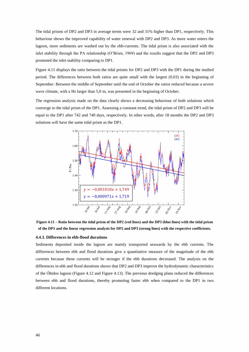
46
The tidal prisms of DP2 and DP3 in average terms were 32 and 31% higher than DP1, respectively. This
behaviour shows the improved capability of water renewal with DP2 and DP3. As more water enters the
lagoon, more sediments are washed out by the ebb-currents. The tidal prism is also associated with the
inlet stability through the PA relationship (O’Brien, 1969) and the results suggest that the DP2 and DP3
promoted the inlet stability comparing to DP1.
Figure 4.11 displays the ratio between the tidal prisms for DP2 and DP3 with the DP1 during the studied
period. The differences between both ratios are quite small with the largest (0,03) in the beginning of
September. Between the middle of September until the end of October the ratios reduced because a severe
wave climate, with a Hs larger than 5,0 m, was presented in the beginning of October.
The regression analysis made on the data clearly shows a decreasing behaviour of both solutions which
converge to the tidal prism of the DP1. Assessing a constant trend, the tidal prism of DP2 and DP3 will be
equal to the DP1 after 742 and 740 days, respectively. In other words, after 18 months the DP2 and DP3
solutions will have the same tidal prism as the DP1.
Figure 4.11 – Ratio between the tidal prism of the DP2 (red lines) and the DP3 (blue lines) with the tidal prism
of the DP1 and the linear regression analysis for DP2 and DP3 (strong lines) with the respective coefficients.
4.4.3. Differences in ebb-flood durations
Sediments deposited inside the lagoon are mainly transported seawards by the ebb currents. The
differences between ebb and flood durations give a quantitative measure of the magnitude of the ebb
currents because these currents will be stronger if the ebb durations decreased. The analysis on the
differences in ebb and flood durations shows that DP2 and DP3 improve the hydrodynamic characteristics
of the Óbidos lagoon (Figure 4.12 and Figure 4.13). The previous dredging plans reduced the differences
between ebb and flood durations, thereby promoting faster ebb when compared to the DP1 in two
different locations.
𝑦 = −0,001010𝑥 + 1,749
𝑦 = −0,000971𝑥 + 1,719
DP2
DP3
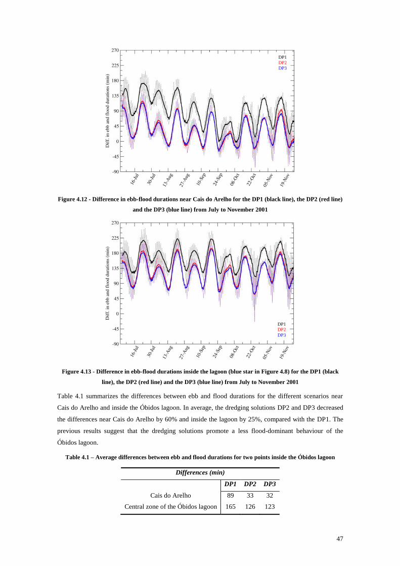
47
Figure 4.12 - Difference in ebb-flood durations near Cais do Arelho for the DP1 (black line), the DP2 (red line)
and the DP3 (blue line) from July to November 2001
Figure 4.13 - Difference in ebb-flood durations inside the lagoon (blue star in Figure 4.8) for the DP1 (black
line), the DP2 (red line) and the DP3 (blue line) from July to November 2001
Table 4.1 summarizes the differences between ebb and flood durations for the different scenarios near
Cais do Arelho and inside the Óbidos lagoon. In average, the dredging solutions DP2 and DP3 decreased
the differences near Cais do Arelho by 60% and inside the lagoon by 25%, compared with the DP1. The
previous results suggest that the dredging solutions promote a less flood-dominant behaviour of the
Óbidos lagoon.
Table 4.1 – Average differences between ebb and flood durations for two points inside the Óbidos lagoon
Differences (min)
DP1 DP2 DP3
Cais do Arelho 89 33 32
Central zone of the Óbidos lagoon 165 126 123
DP1
DP2
DP3
DP1
DP2
DP3
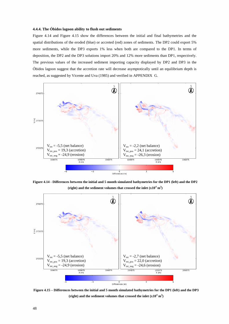
48
4.4.4. The Óbidos lagoon ability to flush out sediments
Figure 4.14 and Figure 4.15 show the differences between the initial and final bathymetries and the
spatial distributions of the eroded (blue) or accreted (red) zones of sediments. The DP2 could export 5%
more sediments, while the DP3 exports 1% less when both are compared to the DP1. In terms of
deposition, the DP2 and the DP3 solutions import 20% and 12% more sediments than DP1, respectively.
The previous values of the increased sediment importing capacity displayed by DP2 and DP3 in the
Óbidos lagoon suggest that the accretion rate will decrease asymptotically until an equilibrium depth is
reached, as suggested by Vicente and Uva (1985) and verified in APPENDIX G.
Figure 4.14 - Differences between the initial and 5 month simulated bathymetries for the DP1 (left) and the DP2
(right) and the sediment volumes that crossed the inlet (x104 m3)
Figure 4.15 – Differences between the initial and 5 month simulated bathymetries for the DP1 (left) and the DP3
(right) and the sediment volumes that crossed the inlet (x104 m3)
Vtot = -5,5 (net balance)
Vtot_pos = 19,3 (accretion)
Vtot_neg = -24,9 (erosion)
Vtot = -2,2 (net balance)
Vtot_pos = 24,1 (accretion)
Vtot_neg = -26,3 (erosion)
Vtot = -5,5 (net balance)
Vtot_pos = 19,3 (accretion)
Vtot_neg = -24,9 (erosion)
Vtot = -2,7 (net balance)
Vtot_pos = 22,0 (accretion)
Vtot_neg = -24,6 (erosion)
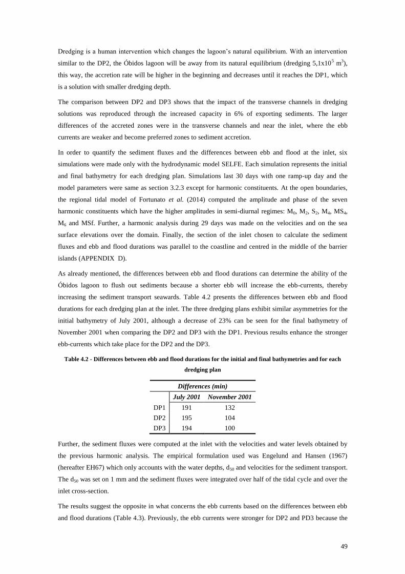
49
Dredging is a human intervention which changes the lagoon’s natural equilibrium. With an intervention
similar to the DP2, the Óbidos lagoon will be away from its natural equilibrium (dredging 5,1x10⁵ m
3),
this way, the accretion rate will be higher in the beginning and decreases until it reaches the DP1, which
is a solution with smaller dredging depth.
The comparison between DP2 and DP3 shows that the impact of the transverse channels in dredging
solutions was reproduced through the increased capacity in 6% of exporting sediments. The larger
differences of the accreted zones were in the transverse channels and near the inlet, where the ebb
currents are weaker and become preferred zones to sediment accretion.
In order to quantify the sediment fluxes and the differences between ebb and flood at the inlet, six
simulations were made only with the hydrodynamic model SELFE. Each simulation represents the initial
and final bathymetry for each dredging plan. Simulations last 30 days with one ramp-up day and the
model parameters were same as section 3.2.3 except for harmonic constituents. At the open boundaries,
the regional tidal model of Fortunato et al. (2014) computed the amplitude and phase of the seven
harmonic constituents which have the higher amplitudes in semi-diurnal regimes: M0, M2, S2, M4, MS4,
M6 and MSf. Further, a harmonic analysis during 29 days was made on the velocities and on the sea
surface elevations over the domain. Finally, the section of the inlet chosen to calculate the sediment
fluxes and ebb and flood durations was parallel to the coastline and centred in the middle of the barrier
islands (APPENDIX D).
As already mentioned, the differences between ebb and flood durations can determine the ability of the
Óbidos lagoon to flush out sediments because a shorter ebb will increase the ebb-currents, thereby
increasing the sediment transport seawards. Table 4.2 presents the differences between ebb and flood
durations for each dredging plan at the inlet. The three dredging plans exhibit similar asymmetries for the
initial bathymetry of July 2001, although a decrease of 23% can be seen for the final bathymetry of
November 2001 when comparing the DP2 and DP3 with the DP1. Previous results enhance the stronger
ebb-currents which take place for the DP2 and the DP3.
Table 4.2 - Differences between ebb and flood durations for the initial and final bathymetries and for each
dredging plan
Differences (min)
July 2001 November 2001
DP1 191 132
DP2 195 104
DP3 194 100
Further, the sediment fluxes were computed at the inlet with the velocities and water levels obtained by
the previous harmonic analysis. The empirical formulation used was Engelund and Hansen (1967)
(hereafter EH67) which only accounts with the water depths, d50 and velocities for the sediment transport.
The d50 was set on 1 mm and the sediment fluxes were integrated over half of the tidal cycle and over the
inlet cross-section.
The results suggest the opposite in what concerns the ebb currents based on the differences between ebb
and flood durations (Table 4.3). Previously, the ebb currents were stronger for DP2 and PD3 because the

50
differences in ebb and flood durations lessened, although, the sediment fluxes for DP2 and DP3 decreased
during the ebb and increased during the flood. However, the EH67 formulation does not account for the
wave orbital velocities neither the current refraction and for that reason, the higher depths of DP2 and
DP3 lead to smaller velocities which were power up by five, thereby decreasing the sediment fluxes at the
inlet for DP2 and DP3.
Table 4.3 – Ratios between the sediment fluxes integrated in half of the tidal cycle (ebb or flood) and in the
inlet cross-section of DP2 and DP3 by DP1 for the initial and final bathymetries
Ratios (-)
July 2001 November 2001
Ebb Flood Ebb Flood
DP2 0,16 0,75 0,65 1,23
DP3 0,15 0,66 0,81 1,18
4.4.5. The application of empirical stability relationships to the Óbidos lagoon inlet
Several empirical relationships are used to predict or to evaluate the stability of an inlet based, for
example, on the tidal prism and on the area of the inlet cross-section. These relationships were already
used over the world, and some of them were presented in section 2.1.2. In this dissertation, it was decided
to perform the application of the PA relationship (Equation 2.2), the Escoffier (1977) diagram and the
Bruun and Gerritssen (1960) criterion to evaluate the stability of the Óbidos lagoon inlet for the different
dredging plans during the studied period.
The PA relationship relates the tidal prism at spring tides with the area of the inlet cross-section. For each
of the six simulations performed in section 4.4.4, the maximum tidal prism during the 29 days and the
area of the inlet cross-section (APPENDIX D) were calculated. The stability curve presented in Figure
4.16 was made with the Jarret (1976) empirical coefficients of 5,02x10⁻⁴
for CPA and 0,84 for n.
Figure 4.16 – Tidal prism-cross-section relationships for the three dredging plans
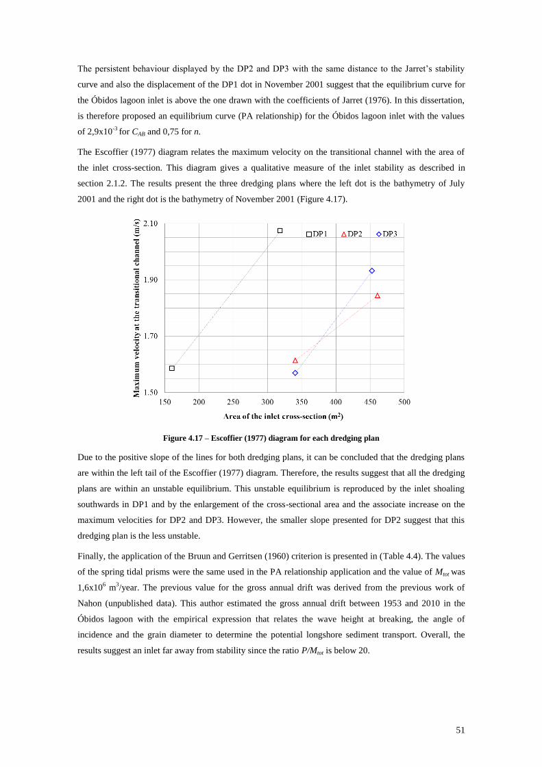
51
The persistent behaviour displayed by the DP2 and DP3 with the same distance to the Jarret’s stability
curve and also the displacement of the DP1 dot in November 2001 suggest that the equilibrium curve for
the Óbidos lagoon inlet is above the one drawn with the coefficients of Jarret (1976). In this dissertation,
is therefore proposed an equilibrium curve (PA relationship) for the Óbidos lagoon inlet with the values
of 2,9x10⁻³
for CAB and 0,75 for n.
The Escoffier (1977) diagram relates the maximum velocity on the transitional channel with the area of
the inlet cross-section. This diagram gives a qualitative measure of the inlet stability as described in
section 2.1.2. The results present the three dredging plans where the left dot is the bathymetry of July
2001 and the right dot is the bathymetry of November 2001 (Figure 4.17).
Figure 4.17 – Escoffier (1977) diagram for each dredging plan
Due to the positive slope of the lines for both dredging plans, it can be concluded that the dredging plans
are within the left tail of the Escoffier (1977) diagram. Therefore, the results suggest that all the dredging
plans are within an unstable equilibrium. This unstable equilibrium is reproduced by the inlet shoaling
southwards in DP1 and by the enlargement of the cross-sectional area and the associate increase on the
maximum velocities for DP2 and DP3. However, the smaller slope presented for DP2 suggest that this
dredging plan is the less unstable.
Finally, the application of the Bruun and Gerritsen (1960) criterion is presented in (Table 4.4). The values
of the spring tidal prisms were the same used in the PA relationship application and the value of Mtot was
1,6x10⁶ m
3/year. The previous value for the gross annual drift was derived from the previous work of
Nahon (unpublished data). This author estimated the gross annual drift between 1953 and 2010 in the
Óbidos lagoon with the empirical expression that relates the wave height at breaking, the angle of
incidence and the grain diameter to determine the potential longshore sediment transport. Overall, the
results suggest an inlet far away from stability since the ratio P/Mtot is below 20.
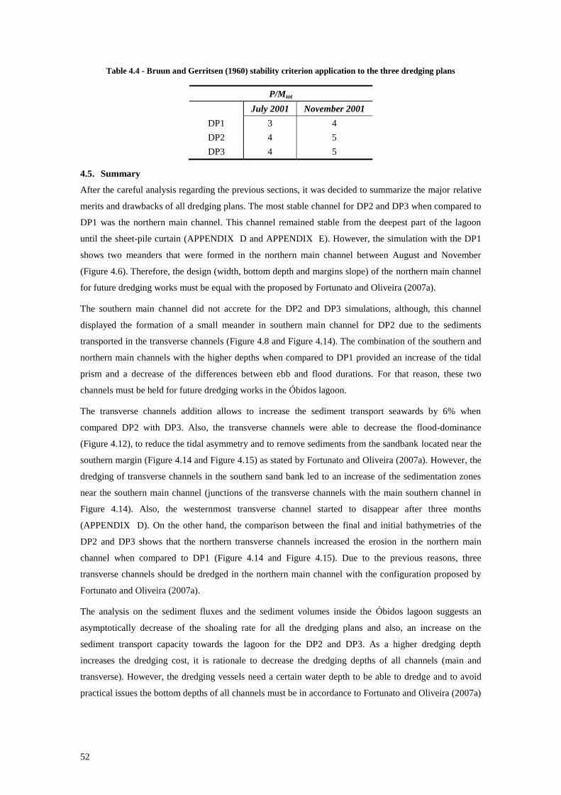
52
Table 4.4 - Bruun and Gerritsen (1960) stability criterion application to the three dredging plans
P/Mtot
July 2001 November 2001
DP1 3 4
DP2 4 5
DP3 4 5
4.5. Summary
After the careful analysis regarding the previous sections, it was decided to summarize the major relative
merits and drawbacks of all dredging plans. The most stable channel for DP2 and DP3 when compared to
DP1 was the northern main channel. This channel remained stable from the deepest part of the lagoon
until the sheet-pile curtain (APPENDIX D and APPENDIX E). However, the simulation with the DP1
shows two meanders that were formed in the northern main channel between August and November
(Figure 4.6). Therefore, the design (width, bottom depth and margins slope) of the northern main channel
for future dredging works must be equal with the proposed by Fortunato and Oliveira (2007a).
The southern main channel did not accrete for the DP2 and DP3 simulations, although, this channel
displayed the formation of a small meander in southern main channel for DP2 due to the sediments
transported in the transverse channels (Figure 4.8 and Figure 4.14). The combination of the southern and
northern main channels with the higher depths when compared to DP1 provided an increase of the tidal
prism and a decrease of the differences between ebb and flood durations. For that reason, these two
channels must be held for future dredging works in the Óbidos lagoon.
The transverse channels addition allows to increase the sediment transport seawards by 6% when
compared DP2 with DP3. Also, the transverse channels were able to decrease the flood-dominance
(Figure 4.12), to reduce the tidal asymmetry and to remove sediments from the sandbank located near the
southern margin (Figure 4.14 and Figure 4.15) as stated by Fortunato and Oliveira (2007a). However, the
dredging of transverse channels in the southern sand bank led to an increase of the sedimentation zones
near the southern main channel (junctions of the transverse channels with the main southern channel in
Figure 4.14). Also, the westernmost transverse channel started to disappear after three months
(APPENDIX D). On the other hand, the comparison between the final and initial bathymetries of the
DP2 and DP3 shows that the northern transverse channels increased the erosion in the northern main
channel when compared to DP1 (Figure 4.14 and Figure 4.15). Due to the previous reasons, three
transverse channels should be dredged in the northern main channel with the configuration proposed by
Fortunato and Oliveira (2007a).
The analysis on the sediment fluxes and the sediment volumes inside the Óbidos lagoon suggests an
asymptotically decrease of the shoaling rate for all the dredging plans and also, an increase on the
sediment transport capacity towards the lagoon for the DP2 and DP3. As a higher dredging depth
increases the dredging cost, it is rationale to decrease the dredging depths of all channels (main and
transverse). However, the dredging vessels need a certain water depth to be able to dredge and to avoid
practical issues the bottom depths of all channels must be in accordance to Fortunato and Oliveira (2007a)

53
except at the inlet where the bottom depth must be +0,0 m (HZ) in order to hamper the sediment transport
towards the lagoon.
Based on the application of the PA relationship to all the dredging solutions, in the case of implementing
the dredging plan proposed by DHI (1997) (DP1), it is also suggested to increase the inlet cross-section
by 100 m2, maintaining the bottom depth and increasing the width in order to have a PA relationship
closer to the proposed stability curve (Figure 4.16).
Overall, the proposed dredging plan for the Óbidos lagoon should have two main channels and three
transverse channels with the configuration proposed by Fortunato and Oliveira (2007a) except the bottom
depth at the inlet which must be dredged to +0,0 m (HZ). Afterwards, the application of the Escoffier
(1977) diagram and the Bruun and Gerritsen (1960) criterion highlighted the fact that without a
permanent solution to stabilize the Óbidos lagoon inlet, this lagoon must be dredged frequently because
its shallow depths and the very energetic wave regime will often drive the inlet to closure.

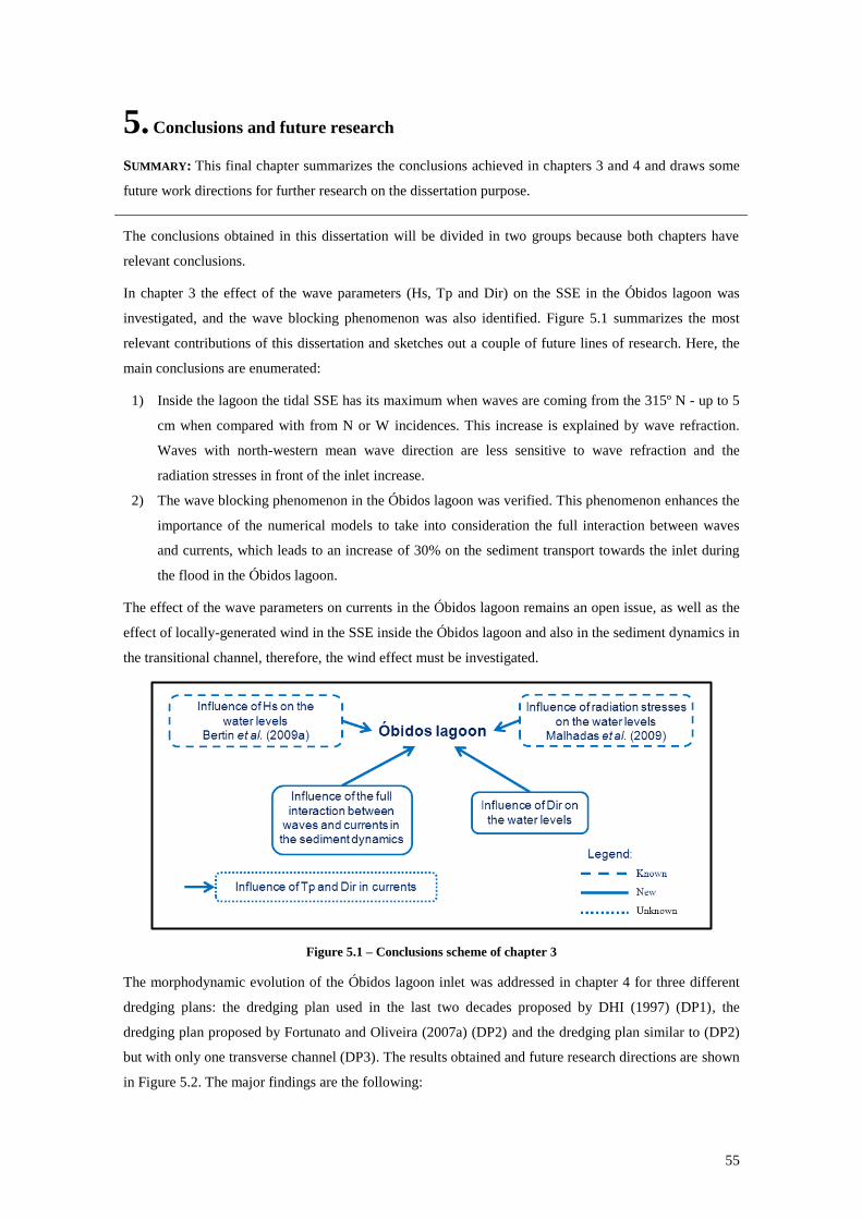
55
5. Conclusions and future research
SUMMARY: This final chapter summarizes the conclusions achieved in chapters 3 and 4 and draws some
future work directions for further research on the dissertation purpose.
The conclusions obtained in this dissertation will be divided in two groups because both chapters have
relevant conclusions.
In chapter 3 the effect of the wave parameters (Hs, Tp and Dir) on the SSE in the Óbidos lagoon was
investigated, and the wave blocking phenomenon was also identified. Figure 5.1 summarizes the most
relevant contributions of this dissertation and sketches out a couple of future lines of research. Here, the
main conclusions are enumerated:
1) Inside the lagoon the tidal SSE has its maximum when waves are coming from the 315º N - up to 5
cm when compared with from N or W incidences. This increase is explained by wave refraction.
Waves with north-western mean wave direction are less sensitive to wave refraction and the
radiation stresses in front of the inlet increase.
2) The wave blocking phenomenon in the Óbidos lagoon was verified. This phenomenon enhances the
importance of the numerical models to take into consideration the full interaction between waves
and currents, which leads to an increase of 30% on the sediment transport towards the inlet during
the flood in the Óbidos lagoon.
The effect of the wave parameters on currents in the Óbidos lagoon remains an open issue, as well as the
effect of locally-generated wind in the SSE inside the Óbidos lagoon and also in the sediment dynamics in
the transitional channel, therefore, the wind effect must be investigated.
Figure 5.1 – Conclusions scheme of chapter 3
The morphodynamic evolution of the Óbidos lagoon inlet was addressed in chapter 4 for three different
dredging plans: the dredging plan used in the last two decades proposed by DHI (1997) (DP1), the
dredging plan proposed by Fortunato and Oliveira (2007a) (DP2) and the dredging plan similar to (DP2)
but with only one transverse channel (DP3). The results obtained and future research directions are shown
in Figure 5.2. The major findings are the following:
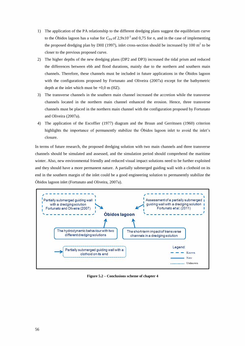
56
1) The application of the PA relationship to the different dredging plans suggest the equilibrium curve
to the Óbidos lagoon has a value for CPA of 2,9x10⁻³
and 0,75 for n, and in the case of implementing
the proposed dredging plan by DHI (1997), inlet cross-section should be increased by 100 m2 to be
closer to the previous proposed curve.
2) The higher depths of the new dredging plans (DP2 and DP3) increased the tidal prism and reduced
the differences between ebb and flood durations, mainly due to the northern and southern main
channels. Therefore, these channels must be included in future applications in the Óbidos lagoon
with the configurations proposed by Fortunato and Oliveira (2007a) except for the bathymetric
depth at the inlet which must be +0,0 m (HZ).
3) The transverse channels in the southern main channel increased the accretion while the transverse
channels located in the northern main channel enhanced the erosion. Hence, three transverse
channels must be placed in the northern main channel with the configuration proposed by Fortunato
and Oliveira (2007a).
4) The application of the Escoffier (1977) diagram and the Bruun and Gerritssen (1960) criterion
highlights the importance of permanently stabilize the Óbidos lagoon inlet to avoid the inlet’s
closure.
In terms of future research, the proposed dredging solution with two main channels and three transverse
channels should be simulated and assessed, and the simulation period should comprehend the maritime
winter. Also, new environmental friendly and reduced visual impact solutions need to be further exploited
and they should have a more permanent nature. A partially submerged guiding wall with a clothoid on its
end in the southern margin of the inlet could be a good engineering solution to permanently stabilize the
Óbidos lagoon inlet (Fortunato and Oliveira, 2007a).
Figure 5.2 – Conclusions scheme of chapter 4
57
Bibliographic references
Abgrall, R. (2006). Essentially non-oscillatory residual distribution schemes for hyperbolic problems.
Journal of Computational Physics, 214(2), 773-808.
Ackers, P., and White, W. R. (1973). Sediment transport: new approach and analysis. Journal of the
Hydraulics Division, 99(11), 2041-2060.
Battjes, J. A. (1974). Computation of set-up, longshore currents, run-up and overtopping due to wind-
generated waves. PhD thesis, Delft University of Technology.
Bennett, N. D., Croke, B. F., Guariso, G., Guillaume, J. H., Hamilton, S. H., Jakeman, A. J., ... and
Andreassian, V. (2013). Characterising performance of environmental models. Environmental
Modelling & Software, 40, 1-20.
Bertin, X., Fortunato, A. B., Oliveira, A. (2009a). A modeling-based analysis of processes driving wave-
dominated inlets, Continental Shelf Research, 29(5), 819-834.
Bertin, X., Fortunato, A. B., Oliveira, A. (2009b). Simulating morphodynamics with unstructured grids:
description and validation of a modelling system for coastal applications, Ocean Modelling, 28 (1),
75-87.
Bertin, X., Fortunato, A. B., Roelvink, D. (2010). Morphodynamic Coastal Environments, 2010 Nova
Science Publishers, Inc.
Bertin, X., Fortunato, A. B., Dodet, G. (2015). Processes controlling the seasonal cycle of wave-
dominated inlets. Journal of Integrated Coastal Zone Management (in press)
Boon III, J. D., and Byrne, R. J. (1981). On basin hypsometry and the morphodynamic response of
coastal inlet systems. Marine Geology, 40(1), 27-48.
Boon, J. D. (2013). Secrets of the tide: tide and tidal current analysis and predictions, storm surges and
sea level trends. Elsevier.
Boothroyd, J. C. (1985). Tidal Inlets and Tidal Deltas. In Coastal Sedimentary Environments. Springer
New York.
Bruneau, N., Fortunato, A. B., Dodet, G., Freire, P., Oliveira, A., Bertin, X. (2011). Future evolution of a
tidal inlet due to changes in wave climate, sea level and lagoon morphology (Óbidos Lagoon,
Portugal). Continental Shelf Research, 31(18), 1915-1930.
Bruun, P., (1978). Stability of Tidal Inlets. Elsevier.
Bruun, P., and F. Gerritsen, (1959). Natural bypassing of sand at coastal inlets. Journal of the Waterways
and Harbors Division, 85, 401–412.
Bruun, P., and F. Gerritsen, (1960). Stability of coastal inlets. Coastal Engineering Proceedings, 1(7), 23.
Camenen, B., & Larson, M. (2005). A general formula for non-cohesive bed load sediment transport.
Estuarine, Coastal and Shelf Science, 63(1), 249-260.
Camenen, B., & Larson, M. (2008). A general formula for noncohesive suspended sediment transport.
Journal of Coastal Research, 615-627.
Castelle, B., Bourget, J., Molnar, N., Strauss, D., Deschamps, S., & Tomlinson, R. (2007). Dynamics of a
wave-dominated tidal inlet and influence on adjacent beaches, Currumbin Creek, Gold Coast,
Australia. Coastal Engineering, 54(1), 77-90.
58
Cayocca, F. (2001). Long-term morphological modeling of a tidal inlet: the Arcachon basin, France.
Coastal Engineering, 42 (2), 115–142.
Consulmar (2008). POOC ALCOBAÇA-MAFRA, Planta de síntese nº3.
Danish Hydraulic Institute, (1997). Projecto para a Fixação da Aberta da Lagoa de Óbidos. Hydraulic
and Sedimentologic Studies. Design of a Dike/Channel System. Relatório Final.
Dean, R.G., Dalrymple, R.A. (2002). Coastal processes with engineering aplications. Cambridge
University Press.
Dias, J. M., Lopes, J. F., & Dekeyser, I. (2000). Tidal propagation in Ria de Aveiro lagoon, Portugal.
Physics and Chemistry of the Earth, Part B: Hydrology, Oceans and Atmosphere, 25(4), 369-374.
Dias, J. M., Sousa, M. C., Bertin, X., Fortunato, A. B., & Oliveira, A. (2009). Numerical modeling of the
impact of the Ancão Inlet relocation (Ria Formosa, Portugal). Environmental Modelling & Software,
24(6), 711-725.
Dinis, J. L., Henriques, V., Freitas, M. C., Andrade, C., Costa, P., (2006), Natural to anthropogenic forcing
in the Holocene evolution of three coastal lagoons (Caldas da Rainha valley, western Portugal),
Quaternary International, (150), 41-51.
Dodet, G., Bertin, X., and Taborda, R. (2010). Wave climate variability in the North-East Atlantic Ocean
over the last six decades. Ocean Modelling, 31(3), 120-131.
Dodet, G., Bertin, X., Bruneau, N., Fortunato, A. B., Nahon, A., and Roland, A. (2013). Wave‐current
interactions in a wave‐dominated tidal inlet. Journal of Geophysical Research: Oceans, 118(3), 1587-
1605.
Dodet., G., (2013). Morphodynamic modelling of a wave-dominated tidal inlet: the Albufeira Lagoon.
PhD thesis, Université de la Rochelle.
Dronkers, J., (1986). Tidal asymmetry and estuarine morphology. Netherlands Journal of Sea Research,
20(2), 117-131.
Engelund, F., and Hansen, E. (1967). A monograph on sediment transport in alluvial streams.
Copenhagen: Teknisk forlag.
Escoffier, F. F., (1977). Hydraulics and stability of tidal inlets. Dept. of Defense, Dept. of the Army,
Corps of Engineers, Coastal Engineering Research Center.
Ferreira, T., Ramos, R., Freitas, M. C., Andrade, C., (2009). Morphological Evolution of the Óbidos
Lagoon (Western Coast of Portugal) Since the Holocene Transgressive Maximum. Journal of Coastal
Research, SI (56), 612-616.
FitzGerald, D. M. (1988). Shoreline erosional-depositional processes associated with tidal inlets. In
Hydrodynamics and Sediment Dynamics of Tidal Inlets (pp. 186-225). Springer New York.
FitzGerald, D. M., N. C. Kraus, and E. B. Hands, (2000). Natural mechanisms of sediment bypassing at
tidal inlets. US Army Corps of Engineers Vicksburg, MS.
Fortunato, A. B., and Oliveira, A. (2000). On the representation of bathymetry by unstructured grids.
Computational Methods in Water Resources XIII, 2, 889-896.
Fortunato, A. B., Freire, P. and Portela, L., (2002). Análise da Implementação do Plano de Gestão
Ambiental da Lagoa de Óbidos: Simulação de Alternativas de Intervenção e Gestão. Report 258/02
NEC, LNEC, Lisboa, (in Portuguese).
59
Fortunato, A. B., and A. Oliveira, (2004a). A modeling system for tidally driven long-term
morphodynamics. Journal of Hydraulic Research, 42 (4), 426–434.
Fortunato, A. B., and A. Oliveira, (2004b). Promoting Ebb Dominance in Coastal Lagoons. Coastal
Engineering Conference, 29 (2), 1173-1885.
Fortunato, A.B., Oliveira, A., (2007a). Case study: promoting the stability of the Óbidos Lagoon inlet.
Journal of Hydraulic Engineering, (133), 816-824.
Fortunato, A. B., Oliveira, A. (2007b). Improving the stability of a morphodynamic modeling system.
Journal of Coastal Research, 50, 486-490.
Fortunato, A. B., Bruneau, N. and Freire, P., (2011). Dragagem e defesa da margem Sul da lagoa de
Óbidos. Resposta às questões levantadas em sede de declaração de impacte ambiental: Aplicação de
um modelo morfodinâmico para analisar a evolução da embocadura. Report 103/11 NEC, LNEC,
Lisboa, (in Portuguese).
Fortunato, A. B. and Portela, L., (2014) Análise pericial da fixação da embocadura da lagoa de Óbidos.
Report 229/14 NEC, LNEC, Lisboa, (in Portuguese).
Fortunato, A. B., Nahon, A., Dodet, G.,… and Oliveira, A., (2014). Morphological evolution of an
ephemeral tidal inlet from opening to closure: The Albufeira inlet, Portugal. Continental Shelf
Research, 73, 49–63.
Freitas, C., (1989). Natureza dos sedimentos do fundo da lagoa de Óbidos, Geolis III (1/2), 144-153 (in
Portuguese).
Freitas, C., Andrade, C., Jones, F. (1992). Recent Evolution of Óbidos and Albufeira Coastal Lagoons. In
Proceedings of the International Coastal Congress, Kiev 1992, 167-186.
Friedrichs, C. T., and D. G., Aubrey, (1988). Non-linear tidal distortion in shallow well-mixed estuaries: A
synthesis. Estuarine Coastal Shelf Science, 27(5), 521–545
Groeneweg, J., Klopman, G., (1998). Changes of the mean velocity profiles in the combined wave current
motion described in a GLM formulation. Journal of Fluid Mechanics, 370, 271-296.
Hasselmann, K., Barnett, T. P., Bouws, E., Carlson, H., Cartwright, D. E., Enke, K., ... and Walden, H.
(1973). Measurements of wind-wave growth and swell decay during the Joint North Sea Wave Project
(JONSWAP). Deutches Hydrographisches Institut.
Hayes, M. O., Goldsmith, V., and Hobbs, C. H. (1970). Offset coastal inlets. Coastal Engineering
Proceedings, 1(12).
Hayes, M. O., (1979). Barrier island morphology as a function of tidal and wave regime. Barrier Islands,
1-27.
Hayes, M. O., FitzGerald, D. M., (2013). Origin, Evolution and Classification of Tidal Inlets. Journal of
Coastal Research, (SI 69), 14-33.
Henriques, M.V. (1997). Dinâmica e protecção da faixa litoral entre a nazaré e Peniche, Colectânea de
Ideias sobre a Zona Costeira de Portugal, Associação EUROCOAST, 553-568.
Hidrotécnica Portuguesa, (1991). Direcção Geral de Portos. Lagoa de Óbidos: Obras de Ligação
Permanente ao Mar. Projecto, Volume 1-Memória Geral, Lisbon (in Portuguese).
60
Hoitink, A. J. F., P. Hoekstra, and D. S., van Maren, (2003). Flow asymmetry associated with
astronomical tides: Implications for the residual transport of sediment. Journal of Geophysical
Research, 108(C10), 1978-2012.
Holthuijsen, L. H. (2007). Waves in oceanic and coastal waters. Cambridge University Press.
Hubbard, D. K., G. Oertel, and D. Nummedal, (1979). The role of waves and tidal currents in the
development of tidal-inlet sedimentary structures and sand body geometry; examples from North
Carolina, South Carolina, and Georgia. Journal of Sedimentary Petrology, 49 (4), 1073–1091.
IH, (2001). Monitorização Ambiental da Lagoa de Óbidos JUL 2001-DEZ 2001. Relatório de Progresso
de Trabalho, Report PT. OC. 06/2001 (in Portuguese).
Jarrett, J., (1976). Tidal prism-inlet area relationships. GITI report 3, Coastal Engineering Research
Center, US Army Corps of Engineers, Fort Belvoir, Virginia.
Jornal das Caldas, (2014). Environment minister assign a contract of 6,5 million for dredging operations
in the Óbidos lagoon (link:
http://jornaldascaldas.com/JournalNews/Journalnewsdetail.aspx?news=f31281ddca7e4808ade832ac2
9f08bdc&q=lagoa consulted in 02/02/2015)
Keller, J. B. (1958). Surface waves on water of non-uniform depth. Journal of Fluid Mechanics, 4(06),
607-614.
Kemp, P.H., Simons, R.R. (1982). The interaction between waves and a turbulent current: waves
propagating with the current. Journal of Fluid Mechanics, 116, 227–250.
Kemp, P.H., Simons, R.R., (1983). The interaction of waves and a turbulent current: waves propagating
against the current. Journal of Fluid Mechanics, 130, 73–89.
Klopman, G. (1994). Vertical structure of the flow due to waves and currents. Progress report H840.30,
Part II. Delft Hydraulics, Delft (The Netherlands).
Komar, P. D., and Miller, M. C. (1975). On the comparison between the threshold of sediment motion
under waves and unidirectional currents with a discussion of the practical evaluation of the threshold:
Reply. Journal of Sedimentary Research, 45(1).
Leonard, B. P. (1991). The ULTIMATE conservative difference scheme applied to unsteady one-
dimensional advection. Computer methods in applied mechanics and engineering, 88(1), 17-74.
Lesser, G. R., Roelvink, J. A., Van Kester, J. A. T. M., and Stelling, G. S. (2004). Development and
validation of a three-dimensional morphological model. Coastal engineering, 51(8), 883-915.
Longuet-Higgins, M. S., and Stewart, R. (1960). Changes in the form of short gravity waves on long
waves and tidal currents. Journal of Fluid Mechanics, 8(04), 565-583.
Longuet-Higgins, M. S., and Stewart, R. W. (1964). Radiation stresses in water waves; a physical
discussion, with applications. In Deep Sea Research and Oceanographic Abstracts (Vol. 11, No. 4, pp.
529-562). Elsevier.
Malhadas, M. S., Leitão, P. C., Silva, A., and Neves, R. (2009). Effect of coastal waves on sea level in
Óbidos Lagoon, Portugal. Continental Shelf Research, 29(9), 1240-1250.
Mehta, A.J., Ozsoy, E., (1978). Inlet hydraulics. In: Bruun, P. (Ed.), Stability of Tidal Inlets: Theory and
Engineering. Elsevier Scientific Publishing Co., Amsterdam, The Netherlands, pp. 83–161.
61
Morang, A., Parson, L. E., (2002). Coastal Morphodynamics. In: Vincent, L., and Demirbilek, Z.
(editors), Coastal Engineering Manual, Part IV, Coastal Geology, Chapter IV-3, Engineer Manual
1110-2-1100, U.S. Army Corps of Engineers, Washington, DC.
Nahon, A., X. Bertin, A. B. Fortunato, and A. Oliveira, (2012). Process-based 2DH morphodynamic
modeling of tidal inlets: A comparison with empirical classifications and theories. Marine Geology,
291-294.
Nielsen, C., and Apelt, C. (2003). The application of wave induced forces to a two-dimensional finite
element long wave hydrodynamic model. Ocean engineering, 30(10), 1233-1251.
Nummedal, D., and Fischer, I. A., (1978). Process-Response Models for Depositional Shorelines: The
German and the Georgia Bights. Proceedings of the Sixteenth Coastal Engineering Conference, 1(16),
ASCE, New York, 1215-1234.
O’Brien, M. P., (1966). Equilibrium flow areas of tidal inlets on sandy coasts. Coastal Engineering
Proceedings, 1(10), Tokyo, Japan.
Olabarrieta, M., Medina, R., Castanedo, S., (2010). Effects of wave-current interaction on the current
profile. Coastal Engineering, 57(7), 643-655.
Oliveira, A., and Fortunato, A. B. (2002). Toward an oscillation-free, mass conservative, Eulerian–
Lagrangian transport model. Journal of Computational Physics, 183(1), 142-164.
Oliveira, A., Fortunato, A.B. e Rego, J.R.L., (2006). Effect of morphological changes on the
hydrodynamics and flushing properties of the Óbidos lagoon (Portugal). Continental Shelf Research,
26(8), 917-942.
Parker, B. B., (1991). The relative importance of the various nonlinear mechanisms in a wide range of
tidal interactions (review). in Tidal Hydrodynamics, edited by B. B. Parker, chap. 13, pp. 237–268,
John Wiley, Hoboken,N. J..
Ranasinghe, R., and C. Pattiaratchi, (1999). The seasonal closure of tidal inlets: Wilson inlet—a case
study. Coastal Engineering, 37 (1), 37–56.
Ranasinghe, R., and Pattiaratchi, C. (2003). The seasonal closure of tidal inlets: causes and effects.
Coastal Engineering Journal, 45(04), 601-627.
Rego, J., (2004). Hidrodinâmica da Lagoa de Óbidos. B.Sc. Thesis for the B.Sc. degree in Geophysical
Sciences – Oceanography, Faculdade de Ciências da Universidade de Lisboa (in Portuguese).
Roelvink, D., Reniers, A., van Dongeren, A. P., van Thiel de Vries, J., McCall, R., and Lescinski, J.
(2009). Modelling storm impacts on beaches, dunes and barrier islands. Coastal Engineering, 56(11),
1133-1152.
Roland, A., (2009), Development of the WWM (Wind Wave Model) II – Spectral Wave Modelling on
Unstructured Meshes. PhD thesis, Technical University of Darmstadt.
Shaeri, S., Tomlinson, R. B., Etemad-Shahidi, A., Strauss, D., and Hughes, L. P. (2014). Hydrodynamics
of a small trained tidal inlet (Currumbin Creek, Australia). Advances in Geosciences, 39, 45-53.
Soulsby, R. (1997). Dynamics of marine sands: a manual for practical applications. Thomas Telford.
Speer, P. E., and D. G. Aubrey, (1985). A study of non-linear tidal propagation in shallow inlet/estuarine
systems. Part II: Theory. Estuarine Coastal Shelf Science, 21(2), 207-224.
Stewart, R. H. (2008). Introduction to physical oceanography. Texas A and M University.
62
Suastika, I. K. (2004). Wave blocking. PhD thesis, Delft University of Technology.
Sutherland, J., Peet, A. H., & Soulsby, R. (2004). Evaluating the performance of morphological models.
Coastal Engineering, 51(8), 917-939.
Teles, M. J., Pires-Silva, A. A., Belo-Pereira, M. (2012). Simulations of wave conditions on open beach
configuration: wind resolution, seaward forcing and whitecapping effects. European Journal
Environmental and Civil Engineering, 16 (8), 927 – 942.
Teles, M.J., Pires-Silva, A.A., Benoit, M., (2013). Numerical modelling of wave current interactions at a
local scale. Ocean Modelling, (68), 7287.
Tolman, H. L. (2002). User manual and system documentation of {WAVEWATCH-III} version 2.22.
Troussellier, M. (Lead Author) and Gattuso, J P., (Topic Editor), 2007. Coastal Lagoons. In: Encyclopedia
of Earth. Eds. Cutler J. Cleveland (Washington, D.C.: Environmental Information Coalition, National
Council for Science and the Environment). (First published in the Encyclopedia of Earth 21.11.2006;
last revised 13.08.2007; retrieved 15.11.2007). (/http://www.eoearth.org/article/Coastal_lagoon
consulted in 16/02/2015).
Umeyama, M., (2005). Reynolds stresses and velocity distributions in a wave–current coexisting
environment. Journal of Waterway, Port, Coastal and Ocean Engineering, 131 (5), 203–212.
United Nations (2013). UN atlas of the oceans.
(http://www.oceansatlas.org/servlet/CDSServlet?status=ND0zNTE4JjY9ZW4mMzM9Ym9v
a3MmMzc9a29z#relateds consulted in 16/02/2015).
Van Rijn, L. C., Walstra, D. J. R., Grasmeijer, B., Sutherland, J., Pan, S., & Sierra, J. P. (2003). The
predictability of cross-shore bed evolution of sandy beaches at the time scale of storms and seasons
using process-based profile models. Coastal Engineering, 47(3), 295-327.
Van Rijn, L. C. (2007a). Unified view of sediment transport by currents and waves. I: Initiation of motion,
bed roughness, and bed-load transport. Journal of Hydraulic Engineering, 133(6), 649-667.
Van Rijn, L. C. (2007b). Unified view of sediment transport by currents and waves. II: Suspended
transport. Journal of Hydraulic Engineering, 133(6), 668-689.
Vão-Arquitectos Associados, (1991). Estudo de recuperação e ordenamento da lagoa de Óbidos, concha
de São Martinho do Porto e orla litoral intermédia, vols. I, II, and V (in portuguese).
Versteeg, H. K., Malalasekera, W., (2007). An introduction to Computational Fluid Dynamics – The
Finite Volume Method. Pearson Education Limited, Edinburgh Gate, England.
Vicente, C. M., Uva, L. P., (1985). Sedimentation in Dredged Channels and Basins – Prediction of
Shoaling Rates. Memória Nº648, LNEC, Lisboa, 1985.
Vieira, J. R., (1984). Mathematical modelling of hydrodynamic and transport processes in coastal regions
– Theoretical and numerical foundations of a two-dimensional circulation model using finite elements.
ITH 13, LNEC, Lisboa, 1984.
Vieira, J. R., (2001). Implementation of the environmental management plano of the Óbidos Lagoon, 2as
Jornadas Portuguesas de Engenharia Costeira e Portuária (CD-ROM), Associação Internacional de
Navegação (in Portuguese).
Vila-Concejo, A., Ferreira, Ó., Matias, A., & Dias, J. M. A. (2003). The first two years of an inlet:
sedimentary dynamics. Continental Shelf Research, 23(14), 1425-1445.
63
Villaret, C., Hervouet, J.-M., Kopmann, R., Merkel, U., Davies, A. G., (2013). Morphodynamic modelling
using Telemac finite-element system. Computers and Geosciences, 53, 105-113.
Vreugdenhil, C. B. (1994). Numerical methods for shallow-water flow. Springer Science & Business
Media.
Walton, T. L., & Adams, W. D. (1976). Capacity of inlet outer ears to store sand. Coastal Engineering
Proceedings, 1(15).
Warren, I., and H. Bach, (1992). MIKE 21: a modelling system for estuaries, coastal waters and seas.
Environmental Software, 7(4), 229–240.
Yanenko, N. N. (1971). The method of fractional steps. Springer-Verlag, New York.
Zhang, Y., and Baptista, A. M. (2008). SELFE: a semi-implicit Eulerian–Lagrangian finite-element model
for cross-scale ocean circulation. Ocean Modelling, 21(3), 71-96.

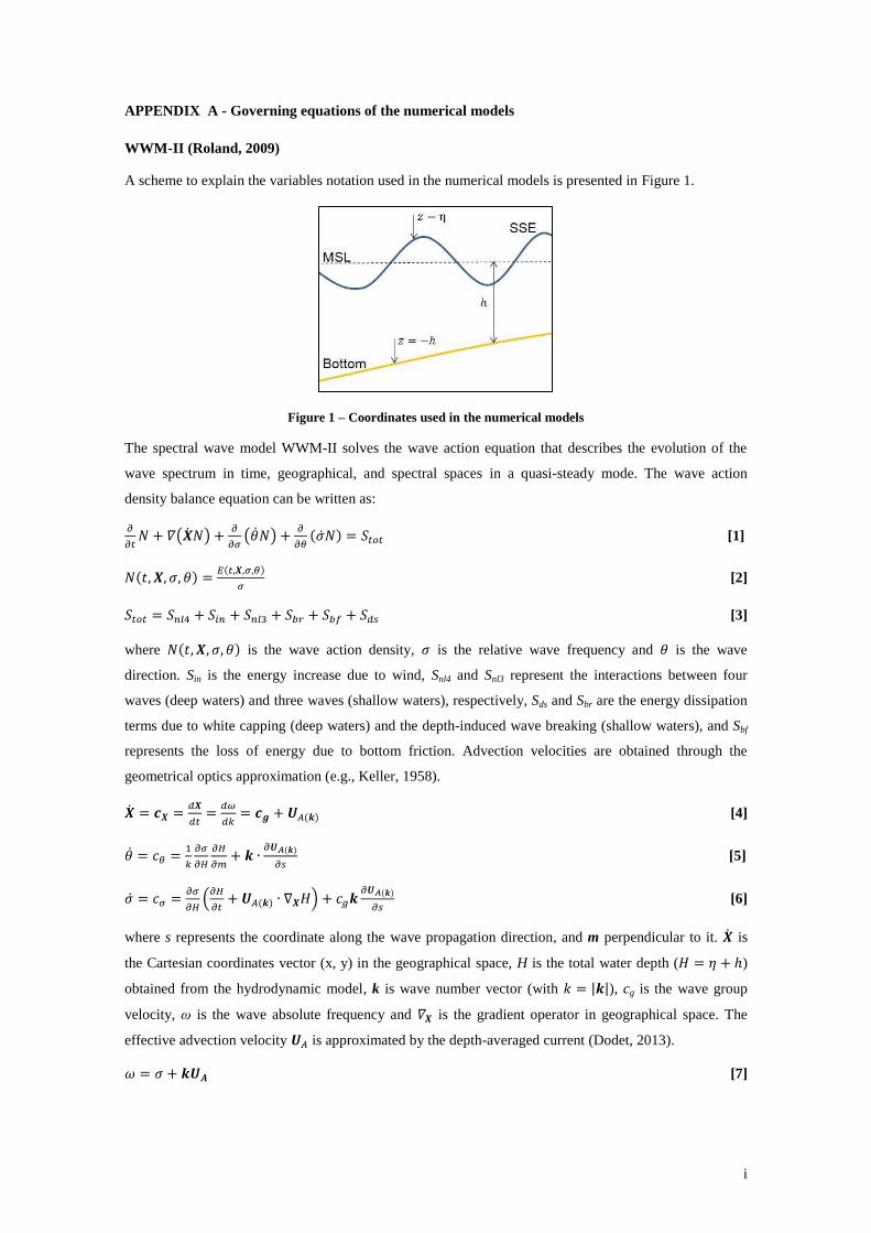
i
APPENDIX A - Governing equations of the numerical models
WWM-II (Roland, 2009)
A scheme to explain the variables notation used in the numerical models is presented in Figure 1.
Figure 1 – Coordinates used in the numerical models
The spectral wave model WWM-II solves the wave action equation that describes the evolution of the
wave spectrum in time, geographical, and spectral spaces in a quasi-steady mode. The wave action
density balance equation can be written as:
𝜕
𝜕𝑡𝑁 + 𝛻(�̇�𝑁) +
𝜕
𝜕𝜎(�̇�𝑁) +
𝜕
𝜕𝜃(�̇�𝑁) = 𝑆𝑡𝑜𝑡 [1]
𝑁(𝑡, 𝑿, 𝜎, 𝜃) =𝐸(𝑡,𝑿,𝜎,𝜃)
𝜎 [2]
𝑆𝑡𝑜𝑡 = 𝑆𝑛𝑙4 + 𝑆𝑖𝑛 + 𝑆𝑛𝑙3 + 𝑆𝑏𝑟 + 𝑆𝑏𝑓 + 𝑆𝑑𝑠 [3]
where 𝑁(𝑡, 𝑿, 𝜎, 𝜃) is the wave action density, 𝜎 is the relative wave frequency and 𝜃 is the wave
direction. Sin is the energy increase due to wind, Snl4 and Snl3 represent the interactions between four
waves (deep waters) and three waves (shallow waters), respectively, Sds and Sbr are the energy dissipation
terms due to white capping (deep waters) and the depth-induced wave breaking (shallow waters), and Sbf
represents the loss of energy due to bottom friction. Advection velocities are obtained through the
geometrical optics approximation (e.g., Keller, 1958).
�̇� = 𝒄𝑿 =𝑑𝑿
𝑑𝑡=
𝑑𝜔
𝑑𝑘= 𝒄𝒈 + 𝑼𝐴(𝒌) [4]
�̇� = 𝑐𝜃 =1
𝑘
𝜕𝜎
𝜕𝐻
𝜕𝐻
𝜕𝑚+ 𝒌 ∙
𝜕𝑼𝐴(𝒌)
𝜕𝑠 [5]
�̇� = 𝑐𝜎 =𝜕𝜎
𝜕𝐻(
𝜕𝐻
𝜕𝑡+ 𝑼𝐴(𝒌) ∙ ∇𝑿𝐻) + 𝑐𝑔𝒌
𝜕𝑼𝐴(𝒌)
𝜕𝑠 [6]
where s represents the coordinate along the wave propagation direction, and m perpendicular to it. �̇� is
the Cartesian coordinates vector (x, y) in the geographical space, H is the total water depth (𝐻 = 𝜂 + ℎ)
obtained from the hydrodynamic model, k is wave number vector (with 𝑘 = |𝒌|), cg is the wave group
velocity, ω is the wave absolute frequency and 𝛻𝑿 is the gradient operator in geographical space. The
effective advection velocity 𝑼𝐴 is approximated by the depth-averaged current (Dodet, 2013).
𝜔 = 𝜎 + 𝒌𝑼𝑨 [7]
ii
The neglected source mechanisms in this dissertation were the four-wave interactions, the white capping
and the wave generation by wind forcing. The domain of this study area is small (approximately 8 to 10
km) and the wind input could be neglected. Therefore, the source terms become:
𝑆𝑡𝑜𝑡 = 𝑆𝑛𝑙3 + 𝑆𝑏𝑟 + 𝑆𝑏𝑓 [8]
Information is shared between SELFE and WWM-II through the radiation stresses induced by waves.
These stresses are obtained with the Longuet-Higgins and Stewart (1960) classical formulation:
𝑅𝑠𝑥 = −1
𝜌0𝐻(
𝜕𝑆𝑥𝑥
𝜕𝑥+
𝜕𝑆𝑥𝑦
𝜕𝑦) [9]
𝑅𝑠𝑦 = −1
𝜌0𝐻(
𝜕𝑆𝒚𝒚
𝜕𝑦+
𝜕𝑆𝑦𝑥
𝜕𝑥) [10]
In Equations 9 and 10, the 𝑆𝑥𝑥 , 𝑆𝑦𝑦 , 𝑆𝑦𝑥 𝑒 𝑆𝑥𝑦correspond to the tensor components of the radiation stresses
which, for an irregular wave spectrum (Battjes, 1974) can be written as:
𝑆𝑥𝑥 = ∫ ∫ 𝑁(𝜎, 𝜃)𝜎 [𝑐𝑔(𝜎)
𝑐𝑝(𝜎)(cos2 𝜃 + 1) −
1
2] 𝑑𝜃𝑑𝜎
2𝜋
0
∞
0 [11]
𝑆𝑦𝑦 = ∫ ∫ 𝑁(𝜎, 𝜃)𝜎 [𝑐𝑔(𝜎)
𝑐𝑝(𝜎)(sin2 𝜃 + 1) −
1
2] 𝑑𝜃𝑑𝜎
2𝜋
0
∞
0 [12]
𝑆𝑥𝑦 = ∫ ∫ 𝑁(𝜎, 𝜃)𝜎𝑐𝑔(𝜎)
𝑐𝑝(𝜎)sin 𝜃 cos 𝜃 𝑑𝜃𝑑𝜎
2𝜋
0
∞
0 [13]
where cp is the wave phase velocity. WWM-II solves Equation 1 with a Fractional Step Method
(Yanenko, 1971). Propagation terms are solved with a Residual Distribution Scheme (Abgrall, 2006).
Spectral advection is solved with the Ultimate Quickest Scheme (Leonard, 1991). A TVD third-order
Runge-Kutta scheme is used for wave breaking and the bottom friction dissipation terms. Triad-wave
interaction uses a dynamic method. For more details on the numerical methods the reader should consult
Roland (2009). For a fully explanation on waves in coastal areas please consult Holthuijsen (2007).
SELFE (Zhang and Baptista, 2008)
The hydrodynamic model SELFE in the depth-averaged version solves the free surface elevation η and
the 2D velocities (u, v) and, in a barotropic configuration, the governing equations in Cartesian
coordinates are:
𝝏𝜼
𝝏𝒕+ 𝜵 ∙ (𝒖𝑯) = 𝟎 [14]
𝑫𝒖
𝑫𝒕= −𝒈𝜵𝜼 + 𝜵 ∙ (𝝁𝜵𝒖) −
𝝉𝒃
𝝆𝟎𝑯− 𝒇(𝒗, −𝒖) + 𝑹𝒔
[15]
where 𝛻 = (𝜕
𝜕𝑥,
𝜕
𝜕𝑦) is the horizontal gradient operator, 𝒖 = 𝒖(𝑥, 𝑦, 𝑡) is the depth-averaged horizontal
velocity with Cartesian components (𝑢, 𝑣), 𝜂 is the free surface elevation, 𝐷
𝐷𝑡 is the total derivative, 𝜇 is
the horizontal turbulent eddy viscosity, 𝝉𝒃 = 𝝉𝒃(𝜏𝑏𝑥 , 𝜏𝑏𝑦) is the bottom stress, 𝑓 is the Coriolis factor, 𝜌0
is the water specific mass and 𝑹𝑠 are the radiation stresses. To review the full derivation of the shallow
water equations please consult Vieira (1984). The bottom stress is computed with a quadratic law:
𝝉𝒃 = (𝜏𝑏𝑥 , 𝜏𝑏𝑦) = 𝜌0𝐶𝐷√𝑢2 + 𝑣2𝒖 [16]
iii
𝐶𝐷 =𝑔𝑛0
2
𝐻1/3 [17]
where 𝐶𝐷 is the bottom drag coefficient and 𝑛0 is the inverse of the Manning coefficient.
SELFE solves Equations 14 and 15 simultaneously through a semi-implicit scheme, dealing with the
advection term trough an Eulerian-Lagrangian Method. With the Garlekin Finite-Element Method, a
positive, symmetric and sparse matrix is obtained. This matrix is solved with the Jacobian Conjugate
Gradient Method. Then, the verification of Equation 14 is done with a Finite Volume Method, ensuring
this way the mass continuity. For more details on the numerical methods the reader should consult
Vreugdenhil (1994). For a fully explanation on the shallow water flows please consult Stewart (2008).
SED2D (Dodet, 2013)
The sediment transport and bottom update model – SED2D – used the Van Rijn (2007a,b) sediment
transport formula which takes into account both the bedload (Equation 18) and the suspended sediment
transport (Equation 19), and is applicable to a wide range of sediments (diameters between 0,05 to 2 mm).
Also, this formula considers the interaction between waves and currents.
𝑞𝑏 = 0,015𝑢𝐻 (𝑑50
𝐻)
1,2
𝑀𝑒1,5
[18]
𝑞𝑠 = 0,012𝑢𝐻𝑑50𝑀𝑒2,4𝐷∗
−0,6 [19]
𝑀𝑒 =𝑢𝑒−𝑢𝑐𝑟
√(𝑠−1)𝑔𝑑502 [20]
where 𝑀𝑒 represents the mobility parameter (Equation 20), 𝑢𝑒 = 𝑢 + 𝛾𝑈𝑤 is the actual speed with
𝛾 = 0,4 in the case of irregular waves and 𝛾 = 0,8 for regular waves, 𝑈𝑤 = 𝜋𝐻𝑠/[𝑇𝑝 sinh(𝑘𝐻)] is the
peak orbital velocity, 𝐻𝑠 is the significant wave height, 𝑇𝑝 is the peak period, 𝑢𝑐𝑟 = 𝛽𝑢𝑐𝑟,𝑐 + (1 −
𝛽)𝑢𝑐𝑟,𝑤 with 𝛽 = 𝑢/(𝑢 + 𝑈𝑤), where 𝑢𝑐𝑟,𝑐 is the critical velocity for currents based on Shields (initiation
of motion) and 𝑢𝑐𝑟,𝑤 is the critical sheer velocity for waves based on Komar and Miller (1975). Critical
shear velocities for waves and currents depend on the sediment median grain diameter (𝑑50) as:
If 0,05 < 𝑑50 < 0,5 mm:
𝑢𝑐𝑟,𝑐 = 0,19(𝑑50)0,1 log(4𝐻/𝑑90) [21]
𝑢𝑐𝑟,𝑤 = 0,24((𝑠 − 1)𝑔)0,66
𝑑500,33(𝑇𝑝)
0,33 [22]
If 0,5 < 𝑑50 < 2 mm:
𝑢𝑐𝑟,𝑐 = 8,5(𝑑50)0,6 log(4𝐻/𝑑90) [23]
𝑢𝑐𝑟,𝑤 = 0,95((𝑠 − 1)𝑔)0,57
𝑑500,43(𝑇𝑝)
0,14 [24]
The bottom update is done through the Exner equation, which is a sediment continuity equation (Equation
25). The Exner equation provides the bottom evolution based on the divergence of the sediment flux field:
𝜕ℎ
𝜕𝑡−
1
1−𝜆∇𝒒 = 0 [25]
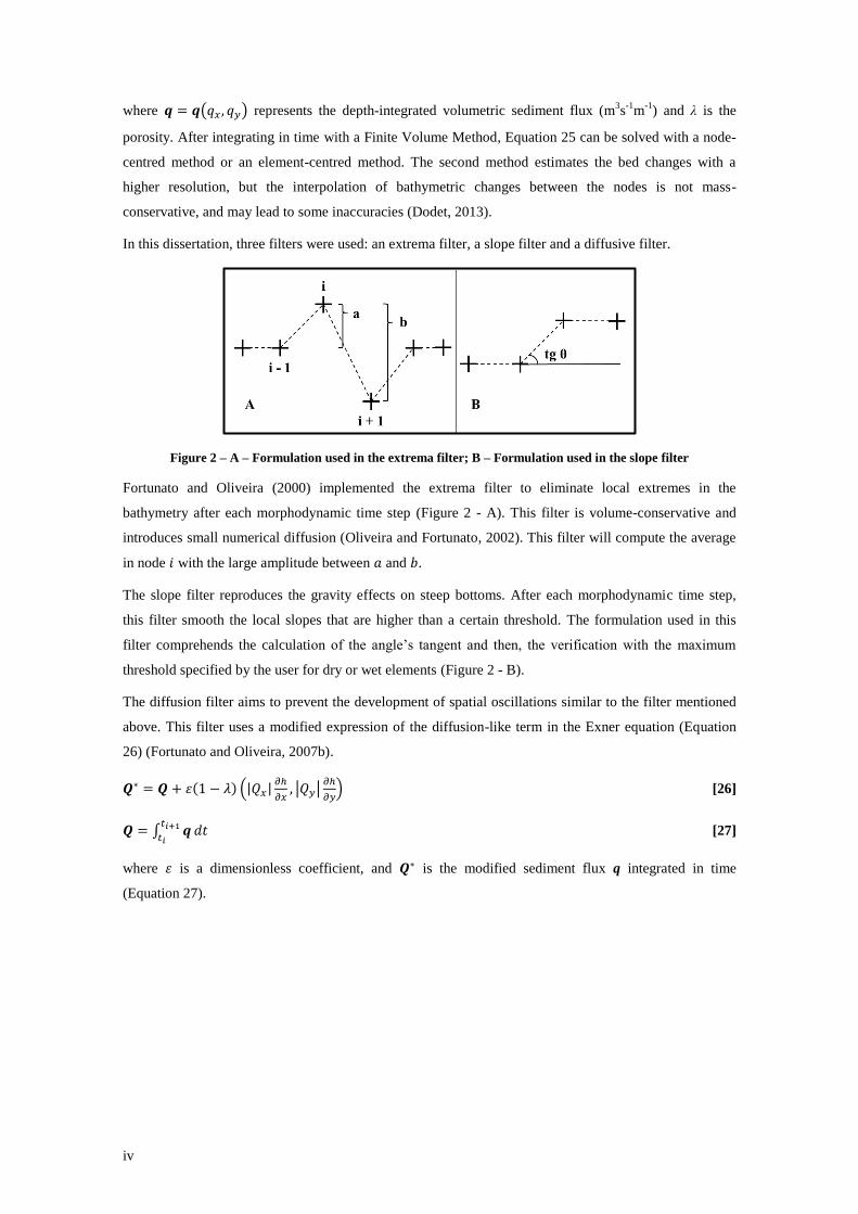
iv
where 𝒒 = 𝒒(𝑞𝑥 , 𝑞𝑦) represents the depth-integrated volumetric sediment flux (m3s
-1m
-1) and λ is the
porosity. After integrating in time with a Finite Volume Method, Equation 25 can be solved with a node-
centred method or an element-centred method. The second method estimates the bed changes with a
higher resolution, but the interpolation of bathymetric changes between the nodes is not mass-
conservative, and may lead to some inaccuracies (Dodet, 2013).
In this dissertation, three filters were used: an extrema filter, a slope filter and a diffusive filter.
Figure 2 – A – Formulation used in the extrema filter; B – Formulation used in the slope filter
Fortunato and Oliveira (2000) implemented the extrema filter to eliminate local extremes in the
bathymetry after each morphodynamic time step (Figure 2 - A). This filter is volume-conservative and
introduces small numerical diffusion (Oliveira and Fortunato, 2002). This filter will compute the average
in node 𝑖 with the large amplitude between 𝑎 and 𝑏.
The slope filter reproduces the gravity effects on steep bottoms. After each morphodynamic time step,
this filter smooth the local slopes that are higher than a certain threshold. The formulation used in this
filter comprehends the calculation of the angle’s tangent and then, the verification with the maximum
threshold specified by the user for dry or wet elements (Figure 2 - B).
The diffusion filter aims to prevent the development of spatial oscillations similar to the filter mentioned
above. This filter uses a modified expression of the diffusion-like term in the Exner equation (Equation
26) (Fortunato and Oliveira, 2007b).
𝑸∗ = 𝑸 + 𝜀(1 − 𝜆) (|𝑄𝑥|𝜕ℎ
𝜕𝑥, |𝑄𝑦|
𝜕ℎ
𝜕𝑦) [26]
𝑸 = ∫ 𝒒𝑡𝑖+1
𝑡𝑖𝑑𝑡 [27]
where 𝜀 is a dimensionless coefficient, and 𝑸∗ is the modified sediment flux q integrated in time
(Equation 27).
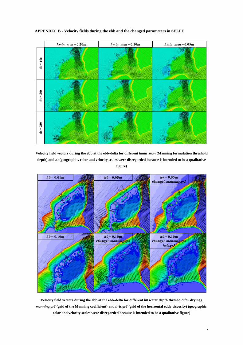
v
APPENDIX B - Velocity fields during the ebb and the changed parameters in SELFE
Velocity field vectors during the ebb at the ebb-delta for different hmin_man (Manning formulation threshold
depth) and Δt (geographic, color and velocity scales were disregarded because is intended to be a qualitative
figure)
Velocity field vectors during the ebb at the ebb-delta for different h0 water depth threshold for drying),
manning.gr3 (grid of the Manning coefficient) and hvis.gr3 (grid of the horizontal eddy viscosity) (geographic,
color and velocity scales were disregarded because is intended to be a qualitative figure)

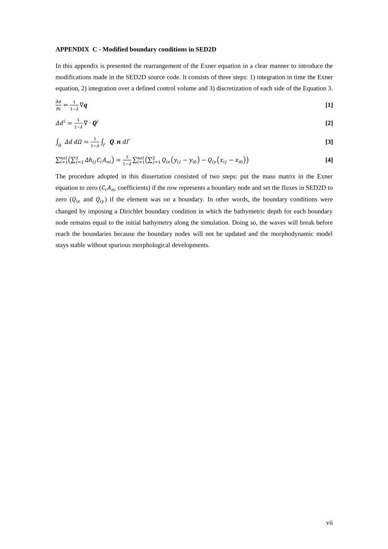
vii
APPENDIX C - Modified boundary conditions in SED2D
In this appendix is presented the rearrangement of the Exner equation in a clear manner to introduce the
modifications made in the SED2D source code. It consists of three steps: 1) integration in time the Exner
equation, 2) integration over a defined control volume and 3) discretization of each side of the Equation 3.
𝜕𝑑
𝜕𝑡=
1
1−𝜆∇𝒒 [1]
𝛥𝑑𝑖 =1
1−𝜆∇ ∙ 𝑸𝑖 [2]
∫ 𝛥𝑑𝛺
𝑑𝛺 =1
1−𝜆∫ 𝑸. 𝒏 𝑑𝛤
𝛤 [3]
∑ (∑ 𝛥ℎ𝑖𝑗𝐶𝑖𝐴𝑛𝑖3𝑗=1 )𝑛𝑒𝑙
𝑖=1 =1
1−𝜆∑ (∑ 𝑄𝑖𝑥(𝑦𝑖𝑗 − 𝑦𝑖0) − 𝑄𝑖𝑦(𝑥𝑖𝑗 − 𝑥𝑖0)2
𝑗=1 )𝑛𝑒𝑙𝑖=1 [4]
The procedure adopted in this dissertation consisted of two steps: put the mass matrix in the Exner
equation to zero (𝐶𝑖𝐴𝑛𝑖 coefficients) if the row represents a boundary node and set the fluxes in SED2D to
zero (𝑄𝑖𝑥 and 𝑄𝑖𝑦) if the element was on a boundary. In other words, the boundary conditions were
changed by imposing a Dirichlet boundary condition in which the bathymetric depth for each boundary
node remains equal to the initial bathymetry along the simulation. Doing so, the waves will break before
reach the boundaries because the boundary nodes will not be updated and the morphodynamic model
stays stable without spurious morphological developments.

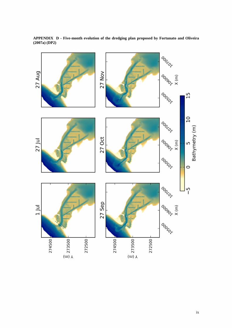
ix
APPENDIX D - Five-month evolution of the dredging plan proposed by Fortunato and Oliveira
(2007a) (DP2)

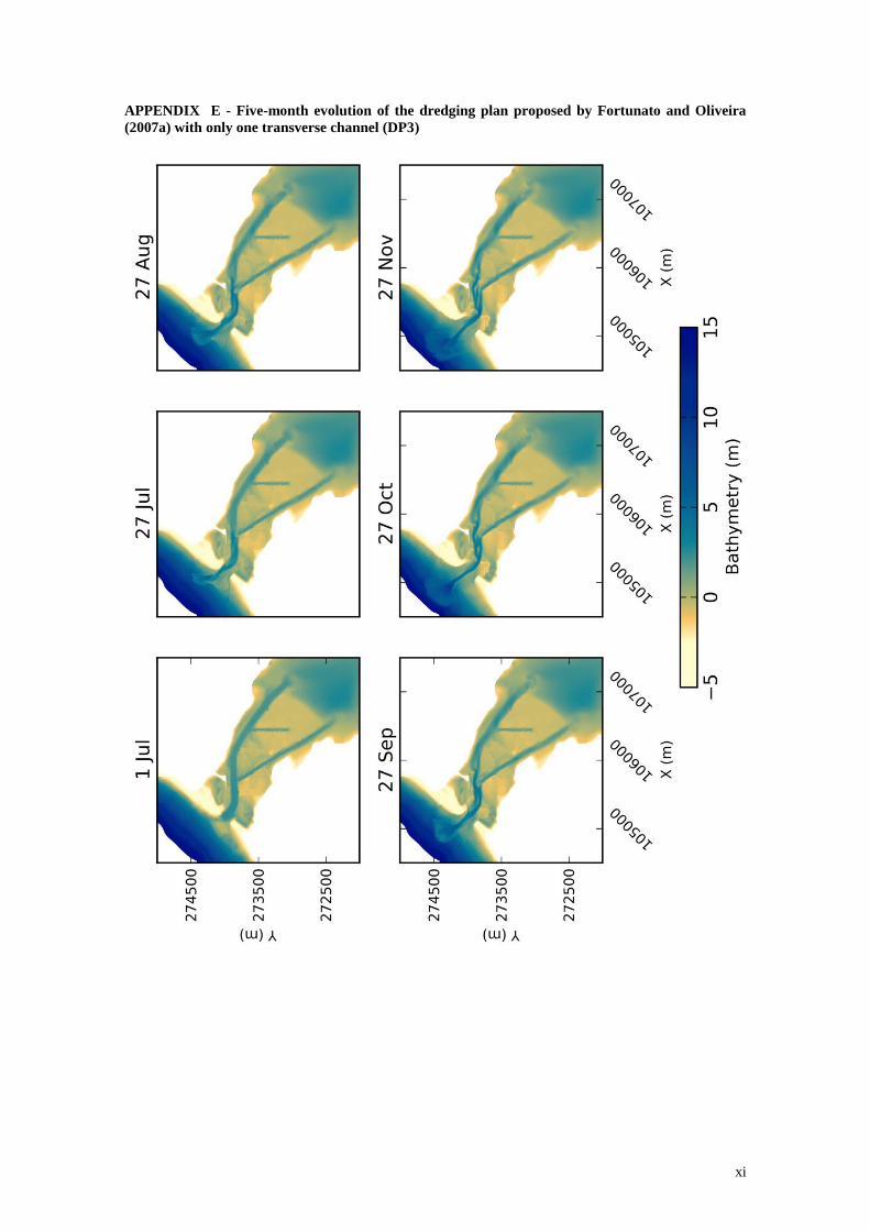
xi
APPENDIX E - Five-month evolution of the dredging plan proposed by Fortunato and Oliveira
(2007a) with only one transverse channel (DP3)

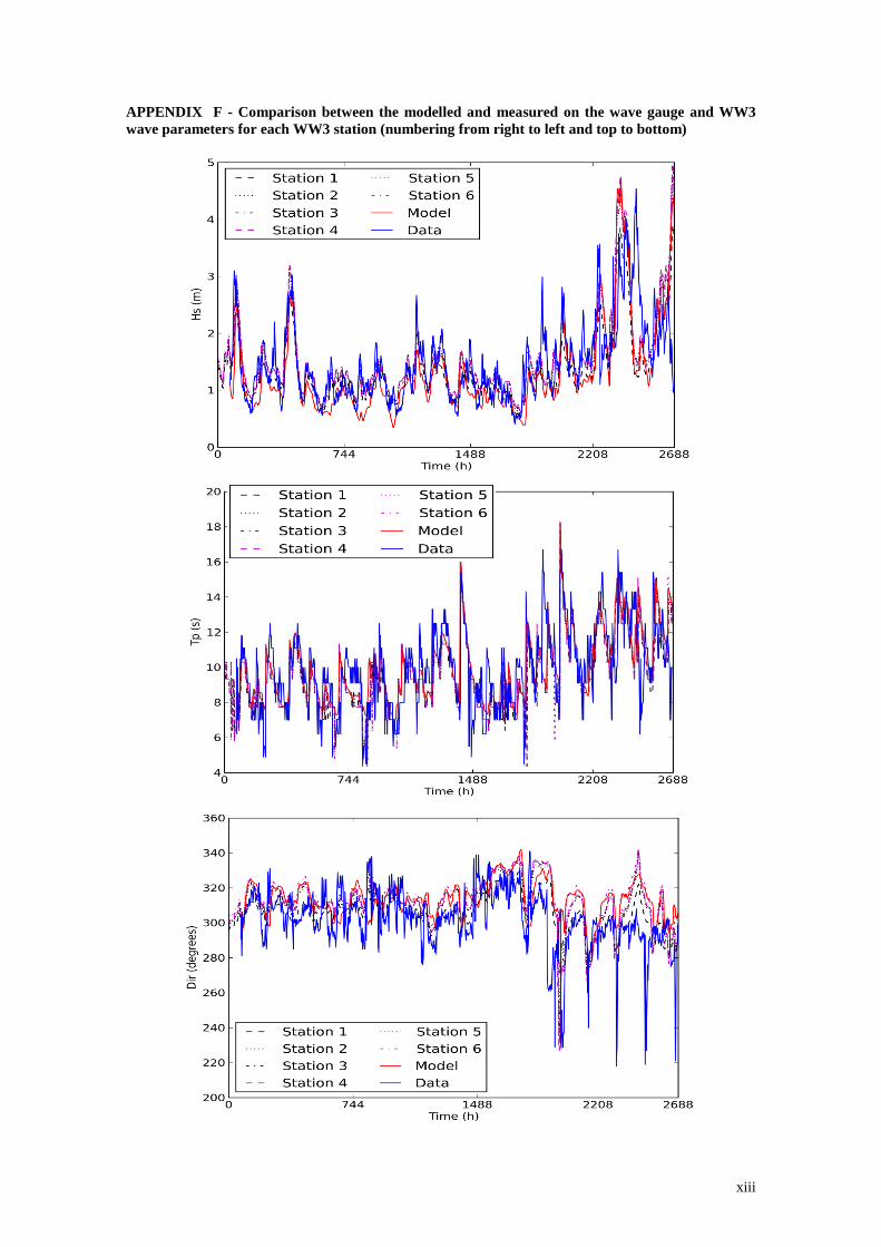
xiii
APPENDIX F - Comparison between the modelled and measured on the wave gauge and WW3
wave parameters for each WW3 station (numbering from right to left and top to bottom)

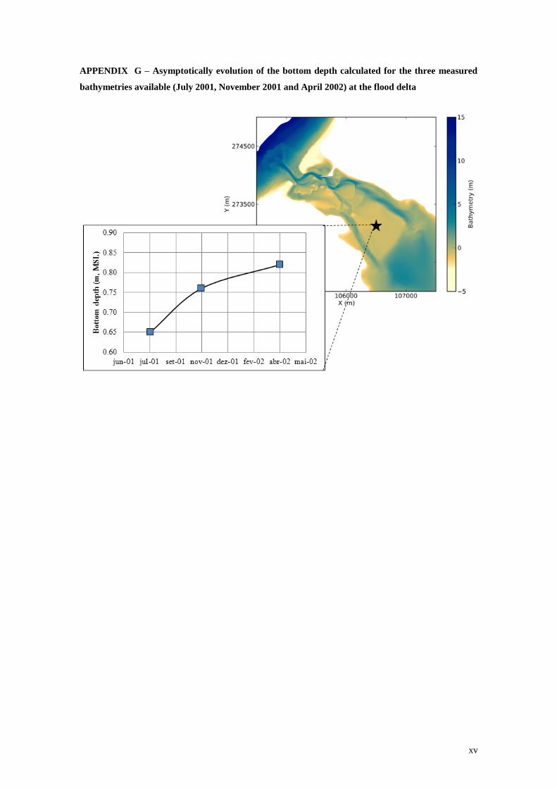
xv
APPENDIX G – Asymptotically evolution of the bottom depth calculated for the three measured
bathymetries available (July 2001, November 2001 and April 2002) at the flood delta