Embed Size (px)
Citation preview
/NASA-CR-124416) A STUDY OF NUMERICAL N73-32762'!METHODS OF SOLUTION OF THE EQUATIONS OFMOTION OF A CONTROLLED SATELLITE UNDERTHE INFLUENCE OF GRAVITY (Mississippi UnclasState Univ.) -. 8" p HC $11.50 CSCL 22C G3/31 15593
airsAEROPHYSICS & AEROSPACE ENGINEERING / MISSISSIPPI STATE UNIVERSITY
A STUDY OF NUMERICAL METHODS OF SOLUTION OF THE EQUATIONS
OF MOTION OF A CONTROLLED SATELLITE
UNDER THE INFLUENCE OF GRAVITY GRADIENT TORQUE
BY
JOE F. THOMPSON
JOHN C. MCWHORTER
SHAHID A. SIDDIQI
SAMUEL P. SHANKS
EIRS-ASE-74-1
https://ntrs.nasa.gov/search.jsp?R=19730024029 2018-08-18T05:50:12+00:00Z
HARRY C. SIMRALL, M.S. COLLEGE ADMINISTRATIONDEAN, COLLEGE OF ENGINEERING
WILLIE L. MCDANIEL, JR., PH.D.ASSOCIATE DEAN
WALTER R. CARNES, PH.D.ASSOCIATE DEAN
LAWRENCE J. HILL, M.S.DIRECTOR, ENGINEERING EXTENSION
CHARLES B. CLIETT, M.S.AEROPHYSICS & AEROSPACE ENGINEERING
WILLIAM R. FOX, PH.D.AGRICULTURAL & BIOLOGICAL ENGINEERING
JOHN L. WEEKS, JR., PH.D.CHEMICAL ENGINEERING
ROBERT M. SCHOLTES, PH.D.CIVIL ENGINEERING
B. J. BALL, PH.D.ELECTRICAL ENGINEERING
W. H. EUBANKS, M.ED.ENGINEERING GRAPHICS
J. E. THOMAS, M.S.INSTITUTE OF ENGINEERING TECHNOLOGY
FRANK E. COTTON, JR., PH.D.INDUSTRIAL ENGINEERING
ALLAN G. WEHR, PH.D.MATERIALS ENGINEERING
C. T. CARLEY, PH.D.MECHANICAL ENGINEERING
JOHN I. PAULK, PH.D.NUCLEAR ENGINEERING
WILLIAM D. MCCAIN, JR., PH.D.PETROLEUM ENGINEERING
For additional copies or informationaddress correspondence to:
ENGINEERING AND INDUSTRIAL RESEARCH STATIONDRAWER DEMISSISSIPPI STATE UNIVERSITYMISSISSIPPI STATE, MISSISSIPPI 39762
TELEPHONE (601)325-2266
iT

A STUDY OF NUMERICAL METHODS OF SOLUTION OF THE EQUATIONS OF MOTION
OF A CONTROLLED SATELLITE
UNDER THE INFLUENCE OF GRAVITY GRADIENT TORQUE
by
Joe F. ThompsonJohn C. McWhorter
Shahid A. Siddiqi
Samuel P. Shanks
Report Number EIRS-ASE-74-1
Prepared by
Mississippi State University
Engineering and Industrial Research Station
Department of Aerophysics and Aerospace Engineering
Mississippi State, Mississippi 39762
Under Contract NAS8-28833
for
NATIONAL AERONAUTICS and SPACE ADMINISTRATION
George C. Marshall Space Flight Center
Marshall Space Flight Center, Alabama 35812
July 1973
/"

TABLE OF CONTENTSPAGE
ABSTRACT. . ........... .. . . ............... 111
INTRODUCTION. . ......... . . .. ............... 1
CHAPTER I - EQUATIONS OF MOTIONS. . ....... . . . . . . 3
CHAPTER II - NUMERICAL EXPERIMENTATION PROCEDURE. . .... . 9
CHAPTER III - RESULTS OF COMPARISON . ........ . . . . 12
Runge-Kutta Methods. . .......... . . . . . . . 12
Multi-step Methods . ........... . . . . . . . 13
Extrapolation Methods. . .......... . . . . . . 15
CHAPTER IV - SURVEY OF TECHNIQUES FOR FURTHER
CONSIDERATION. . .............. .. . 19
Quadrature Methods . ............. . . . . . 19
Multi-value Methods. . ............ . . . . . 22
Non-Polynomial Interpolates. . ............. . 26
Iterative Methods. . ............. . . . . . 27
Transformation Methods . .............. . . 27
Higher-Order Equations . ............... . 27
Conclusions and Directions . ............. . 28
TABLE I . . . . . . . . . . . . . . . . . . . . . . . . . . . 30
TABLE II. . .................. . . . . . . . 31
Figure 1. W 3 and q3 up to T = .25 (quarter of an orbit). . . 32
Figure 2. Errors in W 3 and q 3 versus time, up to T = .04 . . 33
Figure 3. RMS error in W 3 versus step size . ........ 34
Figure 4. Comparison of ERPESR and BSRESH Extrapolation
Methods - Time Step Effects. . ........ .. . 35
Figure 5. Comparison of ERPESR and BSRESH Extrapolation
Methods - Tolerance Effects. . ........ .. . 36
BIBLIOGRAPHY. .............. .... .... . 37
APPENDIX I. . ................. .. ..... . I-1
APPENDIX II ................... ...... .II-1
/1
ABSTRACT
Numerical methods of integration of the equations of motion of a
controlled satellite under the influence of gravity-gradient torque
are considered. The results of computer experimentation using a number
of Runge-Kutta, multi-step, and extrapolation methods for the numeri-
cal integration of this differential system are presented, and par-
ticularly efficient methods are noted. A large bibliography of
numerical methods for initial value problems for ordinary differential
equations is presented, and a compilation of Runge-Kutta and multi-
step formulas is given. Less common numerical integration techniques
from the literature are noted for further consideration.
This report was prepared by Department of Aerophysics and Aerospace
Engineering, Mississippi State University under Contract NAS8-28833 forthe George C. Marshall Space Flight Center of the National Aeronauticsand Space Administration.

INTRODUCTION
The integration of the equations of motion describing the dynamics
of a body in orbit, as affected by various perturbing forces and the
corrective action of control systems, normally requires the use of
hybrid computers because of the difficulty and time involved in inte-
gration of high frequency components by present numerical techniques.
It is desirable, however, to be able to describe the vehicular
dynamics and the vehicle response to control action numerically in order
to take advantage of the advanced development and ease of use of digital
computers, particularly on board the vehicle. This can only be achieved
by improved mathematical analysis of the numerical integration of the
initial value problem with simultaneous ordinary differential equations.
While the numerical techniques that have become standard are adequate
for the integration of such systems when only low frequency modes are
involved, the efficient analysis of high frequency modes requires the
development of new approaches.
It is therefore necessary to develop further the mathematical anal-
ysis of the numerical integration of systems of simultaneous ordinary
differential equations as an initial value problem with specific ap-
plication to the equations describing the vehicular dynamics of a con-
trolled body in orbit. The ultimate goal of the present project is
to develop particularly efficient numerical integration schemes for
the equations of motion of a flexible orbiting body rotating under the
influence of gravity gradient and control torques.
In the present investigation an extensive bibliography of papers
dealing with the numerical solution of systems of ordinary differential
2
equations has been compiled and is included in this report. Many dif-
ferent methods of solution have been obtained therefrom to be compared.
In the present effort comparisons of a large number of Runge-Kutta,
multi-step, hybrid, and extrapolation methods have been made using
the equations of motion of a rigid satellite in circular orbit ro-
tating under the influence of gravity gradient and control torques to
a fixed attitude, and the results of these comparisons are reported
herein. Further effort is required to extend the comparison to other
types of methods, and to compare .ll methods in regard to the equations
of motion of non-rigid satellites.

3
CHAPTER I
EQUATIONS OF MOTION
For a rigid space vehicle in orbit, six ordinary differential
equations are required to specify its spatial motion--three equations
for rotations and three for displacements. If the vehicle is con-
sidered non-rigid,more equations (partial differential equations) are
required to specify the deformations of the body.
In this study the body is considered rigid. The equations of
motion are formulated in terms of quaternions, these being functions
of the direction cosines of the body axes. The introduction of these
quaternions results in seven first order ordinary differential equa-
tions which specify the motion of the body.
The vehicle is in orbit and the motion is assumed to be affected
only by earth's gravitational field. The space vehicle is to be kept
attitude fixed, that is, its direction should be invariant for all time.
Any deviations from this fixed direction are to be corrected by an
on-board control system. Deviations from the fixed attitude occur
because of the gravity gradient and imperfections in the launch
process. These deviations are indicated by the quaternions.
The seven first-order ordinary differential equations, in matrix
form are:
3GMIw + w x IIw = - r I*r + T 1.1 (3 equations)
ll -- c
S= - 1 2(w)q 1.2 (4 equations)2 - -

where
w = w2 is the angular velocity vector,
w
w is the time rate of change of w,
q1 el1sin i/2
q2 e2sin /2= is the quaternion vector,
q3 e3sin /2
q cos i/2
is the time rate of change of q,
is the angle of rotation of the body's rotation vector e from a fixed
attitude,
T is the control torque vector, a function of w and j,
i11 i12 i13
S= 21 i22 i23 is the moment of inertia matrix
i31 i32 i33
r is the radius vector of the orbit referred to the vehicle fixed
axes and is related to the inertial axes, fixed to the center of
the earth, by a transformation matrix D,
G is the universal gravitational constant,
M is the mass of the earth,
(w) is an asymmetric matrix function of w as defined below:

5
0 -w 3 W2 W1
w3 0 - I w2
M(w) = 2 1 0-w2 wI w3
-Wl 2 -W3 0
Since I is non-singular, we may write (1.1) as
w = I-1 [ 3GM x r - w x w + T] 1.3
Evaluating the matrix cross products and defining an asymmetric
matrix function F(a), where a is any vector, by
0 -a3 a2
F(a) = a3 0 -l
-a2 a1 0
we have
-1 3GMw = I [ F(r)I r- F(w)I w + Tc] 1.4
* 11= - (w) 1.52
The transformation of rI (inertial axes) to r (vehicle axes) is
given by
cos w0t
S R sin wt 1.6I 0
0 /
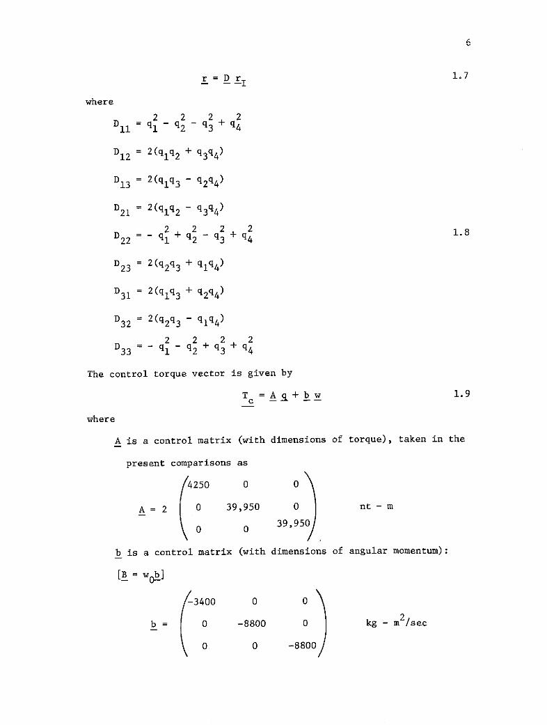
r =D r I 1.7-I
where
2 2 2 2D11 =1 - 2 - 3 + 4
D12 = 2(qlq2 + q 3 q 4 )
D13 = 2(qlq3 - q 2 q 4 )
D21 = 2(qlq 2 - q 3 q 4 )
D -2 2 2 2 1.822 = 1
+ q2 - q3 + 4
D23 = 2(q 2 q 3 + q 1 q 4 )
D31 = 2(qlq 3 + q2 q4 )
D32 = 2(q 2q3 - q1 q4 )
2 2 2 233 1- 2 + 3 +4
The control torque vector is given by
T =A +b w 1.9
where
A is a control matrix (with dimensions of torque), taken in the
present comparisons as
4250 0 0
A = 2 0 39,950 0nt - m
0 0 39,95
b is a control matrix (with dimensions of angular momentum):
[B = w b]
-3400 0 0
b = 0 -8800 0kg - m2/sec
0 0 -8800
7
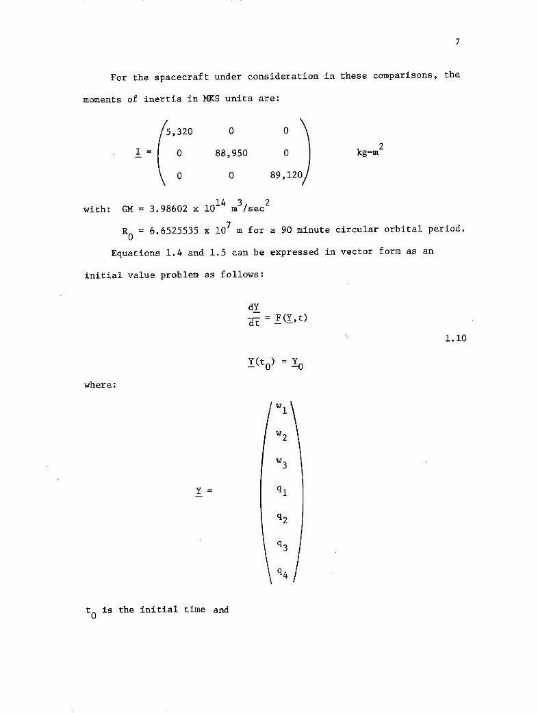
For the spacecraft under consideration in these comparisons, the
moments of inertia in MKS units are:
,320 0 0
= 88,950 0kg-m 2
0 0 89,120
w= 14 3 2
with: GM = 3.98602 x 10 m /sec
RO = 6.6525535 x 10⁷ m for a 90 minute circular orbital period.
Equations 1.4 and 1.5 can be expressed in vector form as an
initial value problem as follows:
dY
dt- F(Y,t)
1.10
Y(t0 ) =
where:
w2
w3
Y= q1
q2
q3
q4
t0 is the initial time and

wwl(t 0)
w2 (t O)
w3 (t 0)
1 (t 0
q 2 (t 0 )
q 3 (t 0 )
q 4(to)
9
CHAPTER II
NUMERICAL EXPERIMENTATION PROCEDURE
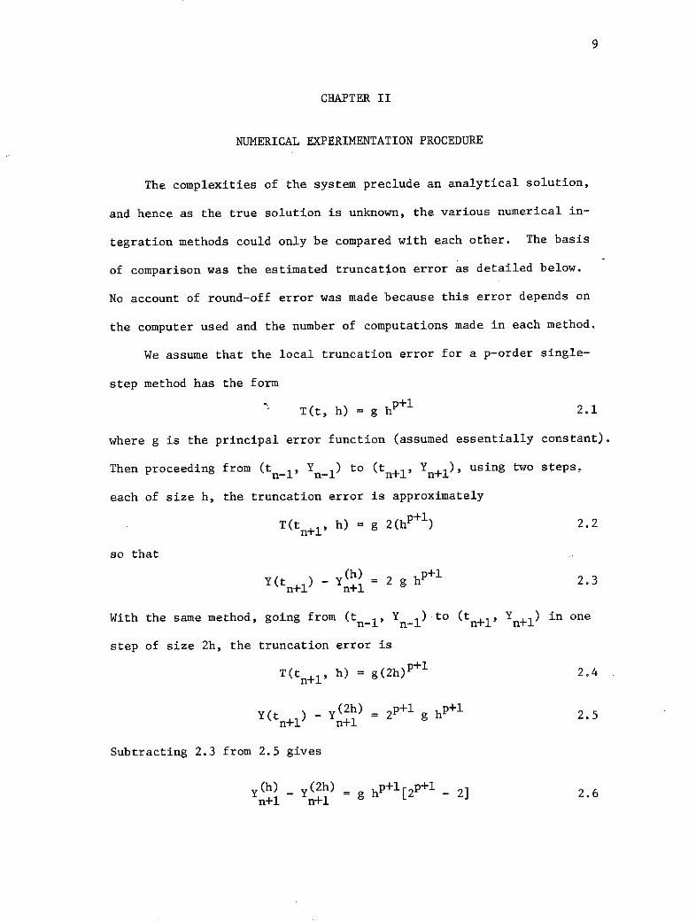
The complexities of the system preclude an analytical solution,
and hence as the true solution is unknown, the various numerical in-
tegration methods could only be compared with each other. The basis
of comparison was the estimated truncation error as detailed below.
No account of round-off error was made because this error depends on
the computer used and the number of computations made in each method.
We assume that the local truncation error for a p-order single-
step method has the form
T(t, h) = g hp+l 2.1
where g is the principal error function (assumed essentially constant).
Then proceeding from (tn 1 Yn-l) to (tn+l Y n+l ) , using two steps,
each of size h, the truncation error is approximately
T(tn+l, h) = g 2(h p+ 1) 2.2
so that
(h) p+lY(t ) - Y = 2 g h 2.3
n+1 n+1
With the same method, going from (tn-, n-1) to (tn+1 Yn+l ) in one
step of size 2h, the truncation error is
T(tn+, h) = g(2h)p+l 2.4
(2h) p+l p+lY(t ) - Y2h) 2 l g h 2.5
n+1 n+1
Subtracting 2.3 from 2.5 gives
y(h) _(2h) P+lp+Y (h)- Y g h [2p + - 2] 2.6n+l n+l

10
Then approximately (h) - (2h)n+l n+l
T(t h) =n+l n+ 2.7n+l' 2P+1 - 2
Equation 2.7 was used to compare different methods. This is not
an exact expression for the truncation error because g is not completely
constant. Still this expression is a useful way to compare methods be-
cause it gives some measure of the truncation error involved. This
estimate applies strictly to single-step methods, but was used for all
methods since it still is some measure of the error and should tend
to zero for any method as the step size decreases to zero even though
it is not strictly to be interpreted as truncation error for multi-
step methods.
Each method tested was run for the maximum step size, and then
a number of runs were made with the step size halved successively.
Equation 2.7 was used to estimate the error between the solution using
step size h, and the solution using h/2. This error was calculated at
each time step and a root mean square of these errors was calculated.
This RMS value was used to judge different methods.
The initial conditions used for the comparison were
0 0
((t 0 q(t) = 0
1
The period of orbit was 90 minutes. The maximum step size used was
h = 0.001.*
*All times and time steps without units are fractions of the orbit
period.

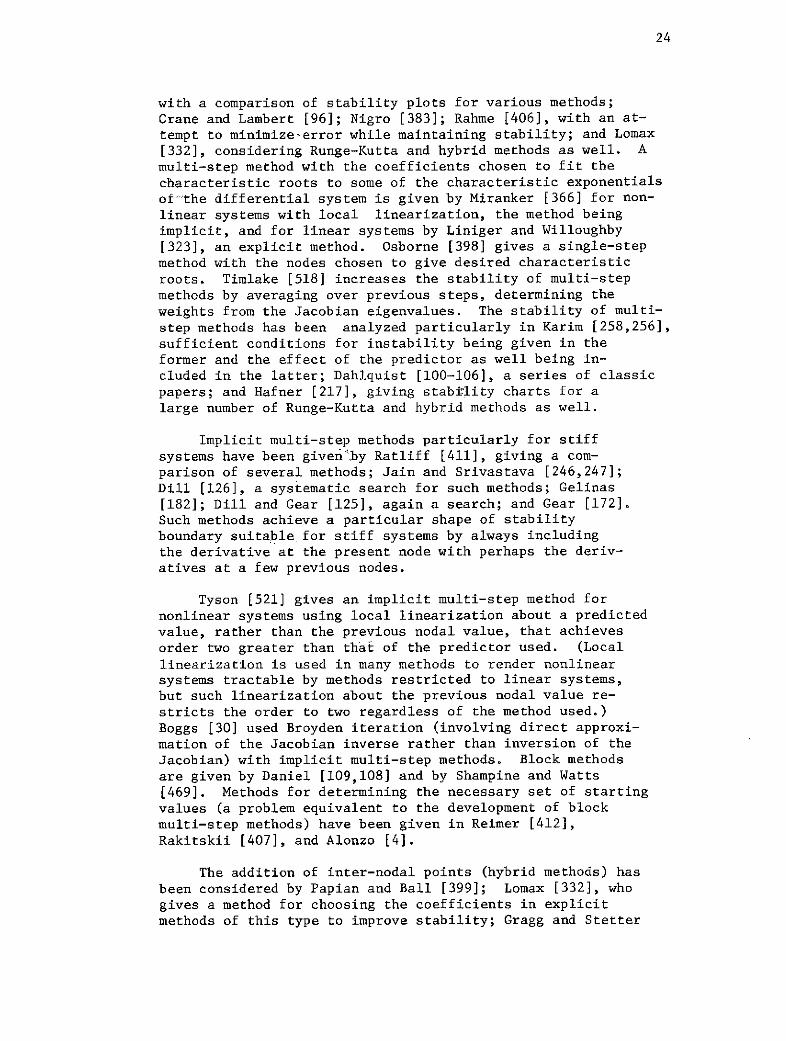
Figure 1 illustrates a typical solution up to t = 0.25 (quarter
of an orbit).
With the initial conditions used, wl, w2, q1 ' q2 ' q4 always re-
main unchanged, while w3 and q3 oscillate. This is to be expected as
the gravity differential on the spacecraft is the only disturbing
moment, and hence only w3 and q3 are affected. q3 oscillates at twice
the orbital period, and has no transient phase. w 3, however, has a
transient phase, and dictates the step size, h, necessary for stability.
For this reason, only the truncation error committed in w3 was used to
judge the methods tested. The error in w3 by far outweighs the error
in q3 '
Most methods were unstable for h = 0.001. With each method six
more h's were run, with h halved for each run. Figure 1 shows that
the fast ocsillations of w3 die down at about t = 0.02. The comparison
scheme discussed above was used to calculate the RMS truncation error
up to t = 0.04. This interval includes a period of fast oscillation,
up to t = 0.02, and a period of slow periodic oscillation, up to t =
0.04. The h = 0.001 runs will obviously have the maximum truncation
error, and each successive halving of h will reduce this error because
as h + 0 the truncation error -* 0.
All runs were made in single precision arithmetic on a UNIVAC
1106 computer.
12
CHAPTER III
RESULTS OF COMPARISONS
Runge-Kutta Methods*
In Table I Runge-Kutta methods are compared by two parameters:
RMS truncation error and computational time. The computational time
is calculated as the number of function evaluations required by the
particular method, i.e., the number of stages, V, for Runge-Kutta
methods. Thus computation time is in units of number of function
evaluations. Each method compared is identified by its name and
its equation number in Appendix I.*
An X under a step size h, indicates that the method was unstable
for that h. A - under a step size h, indicates that this step size
was not run with this method. A 0 will occur for the smallest step
size run because no truncation error can be calculated for the smallest
step size.
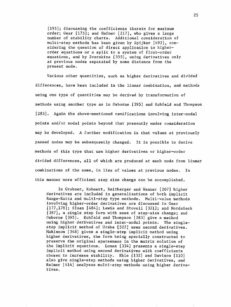
Figure 2 shows examples of the errors in w 3 and q3 for various
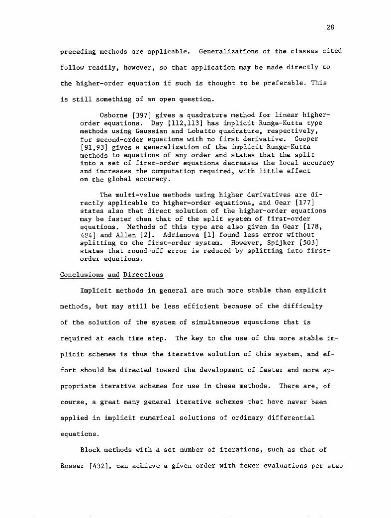
step sizes plotted against time t. Figure 3 shows examples of the
RMS T plotted against step size for w 3. Both these figures are for
the fourth-order Runge-Kutta-Ralston method.
Selecting a best method out of the ones tested is a judgment
problem and depends on the users' requirements. Most users require
both speed and accuracy. Hence the methods of Table I were judged
on the basis of an error-time parameter,ET. This is a judgment
*Shahid Ahmed Siddiqi, "A Comparison of Various Order, Single-Step Explicit Runge-Kutta Methods Used to Solve the Equations ofMotion of a Rigid Spacecraft in Circular Orbit" (unpublished M.S.thesis, Mississippi State University, 1973).
13
?arameter which gives an equal weight to both the error and the compu-
tational time of a particular method:
REMS T VET = P+ ) )
2 - 2
Based on this parameter, ET, the following observations are im-
mediately made from Table I:
Best fourth-order RKE: Ralston RKE(4,4)*
Best fifth-order RKE: Butcher RKE(5,6)
Best sixth-order RKE: Shanks RKE(6,6)
Best seventh-order RKE: Sarafyan RKE(7,10)
(except for h = 0.000125)
Best eighth-order RKE: Shanks RKE(8,10)
(except for h = 0.000125)
Now from among these five methods, the best choice, based on
the ET parameter, is Shanks RKE(8,10) with h = 0.00025.
The results can be interpreted in another way: it is better,
i.e., smaller ET, to use the Butcher RKE(5,6) at h = 0.000125 than
to use the Shanks RKE(8,10) at h = 0.0005. Another observation,
evident from Table I,is that the sixth, seventh, and eighth-order
methods reach minimum ET's, but not at the smallest step size.
It is again emphasized that the judgment parameter ET gives equal
weight to error and time.
Multi-Step Methods
Although a complete investigation of the multi-step methods is
desirable, the available time permitted only a limited investigation.
*RKE(q,r) refers to an explicit Runge-Kutta method of q-order withr stages.

14
With the time factor in mind, three of the most promising types of
predictors were chosen - Adams-Bashforth (AB), Krough, and Craine-
Klopfenstein (CK), and three types of correctors were chosen -
Adams-Moulton (AM), Rodabough-Wesson (RW) and Wesson. Also, a Butcher
fifth order hybrid method was chosen to compare with the multi-step
methods.
The predictor and corrector equations were used to solve the
initial value problem in various P-C combinations in both the PEC and
PECE modes. Also the PE(CE) s mode was run with an accelerated Jacobi
scheme; however, the acceleration parameter was found to be zero for
this solution. Thus, the PE(CE) s mode was discarded. The result
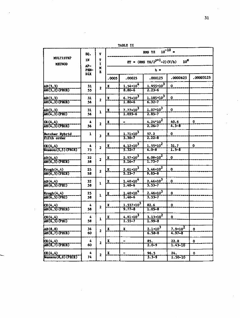
of the experimentation is presented in Table II.
From Table II, the best of the three types of predictors was
the CK predictor, and the best of the three types of correctors was
the AM corrector. To verify these conclusions the following observa-
tions were made:
1) The three predictors were used in P-C combinations with the
sixth-order AM corrector. The fourth-order CK was found
to give a truncation error 9.4 times less than that of the
fourth-order Krogh predictor for a time step of .000125.
Also, the fourth-order CK was found to give a truncation
error 16.5 times less than that of the fourth-order AB
predictor at the same time step.
2) The fifth-order Butcher hybrid gave 3 times less truncation
error than the eighth-order AB-AM combination for a time
step of .000125. However, the sixth-order CK-AM combination
gave 2 times less truncation error than the fifth-order
Butcher hybrid method.

15
3) The fourth-order CK-sixth-order AM combination gave 6.5 times
less truncation error than the eighth-order AB-AM combination.
4) The RW correctors gave solutions that did not closely compare
with the other Runge-Kutta and multi-step solutions. Thus,
the RW correctors were discarded.
5) The fourth-order CK-eighth-order AM combination had slightly
less truncation error than the fourth order CK-eighth-order
Wesson combination for all timesteps considered.
Based on the merit factor, ET, introduced above, the fourth-
order CK-eighth-order AM combination is the best of those considered.
The best multi-step methods considered are generally less ef-
fective than the best Runge-Kutta methods when judged by this merit
factor, and stability limitations preclude the use of the larger
step sizes allowed with the Runge-Kutta methods with the higher-
order methods. It thus appears that the best Runge-Kutta methods are
to be preferred for this system of differential equations.
Extrapolation Methods
Six extrapolation methods were investigated. These methods used
rational function and polynomial function extrapolation with the
Euler and modified midpoint algorithms. The Euler algorithm was
used with polynomial function extrapolation with the basic time step
being subdivided according to each of the sequences
hk = h0/2k
and
hk = {h0 , h0/2, h0/3, h0 4, ... }
The modified midpoint rule was used with both rational function and
polynomial function extrapolation with each of the above sequences.

16
All methods used local extrapolation. The A-stable trapezoidal rule
was not used since it requires global extrapolation. Further details
on the Euler-Romberg and Bulirsch-Stoer modified midpoint method
can be found in Reference [556].
Since the extrapolation methods subdivide each time step re-
peatedly until a desired tolerance between successive extrapolations
is obtained, comparisons with other methods is not directly possible.
However, some conclusions can be drawn concerning the best of the
extrapolation methods with regard to accuracy and number of function
evaluations.
Extrapolation methods have as variable parameters the basic step
size and the tolerance between successive extrapolations. In this
work there is no automatic step size correction. Results for compari-
son purposes were obtained by making a number of computer runs at
different basic step sizes with constant tolerance between successive
extrapolations and then repeating the runs with successively smaller
tolerances between successive extrapolations. These results indicate
an optimum value of tolerance and step size for each method. As the
basic step size increases, the number of extrapolations (function
evaluations) needed to obtain a given tolerance decreases. However,
for large step sizes the accuracy of the extrapolated values tends
to decrease. The optimum values must be determined for each method
experimentally. If the tolerance between successive extrapolations
is too low, accuracy is poor, while if too high, instability can occur.
All midpoint rule methods became unstable at a basic step size
of .00037 (fraction of one orbit), some at a smaller step size. So
apparently extrapolation cannot totally overcome the instability
17
characteristic of the midpoint rules. When using a halving sequence,
polynomial function extrapolation required more function evaluations
than the rational function extrapolation with little difference in
accuracy. If a reciprocal sequence was used the polynomial function
extrapolation required fewer function evaluations than the rational
function extrapolation method but gave less accurate results and
went unstable at a lower step size. Thus there is little advantage
to either rational function or polynomial function extrapolation, and
the reciprocal and halving sequences produced no real savings in
function evaluations when used with the midpoint rule.
Of the two Euler methods which both used polynomial function ex-
trapolation, the solution obtained with the reciprocal sequence was
very slightly more accurate than the solution obtained by successively
halving the time step. The number of function evaluations was from
2 to 8 times fewer for the solution with the reciprocal sequence of
step size subdivision, depending upon the smallness of the tolerance
between successive extrapolations.
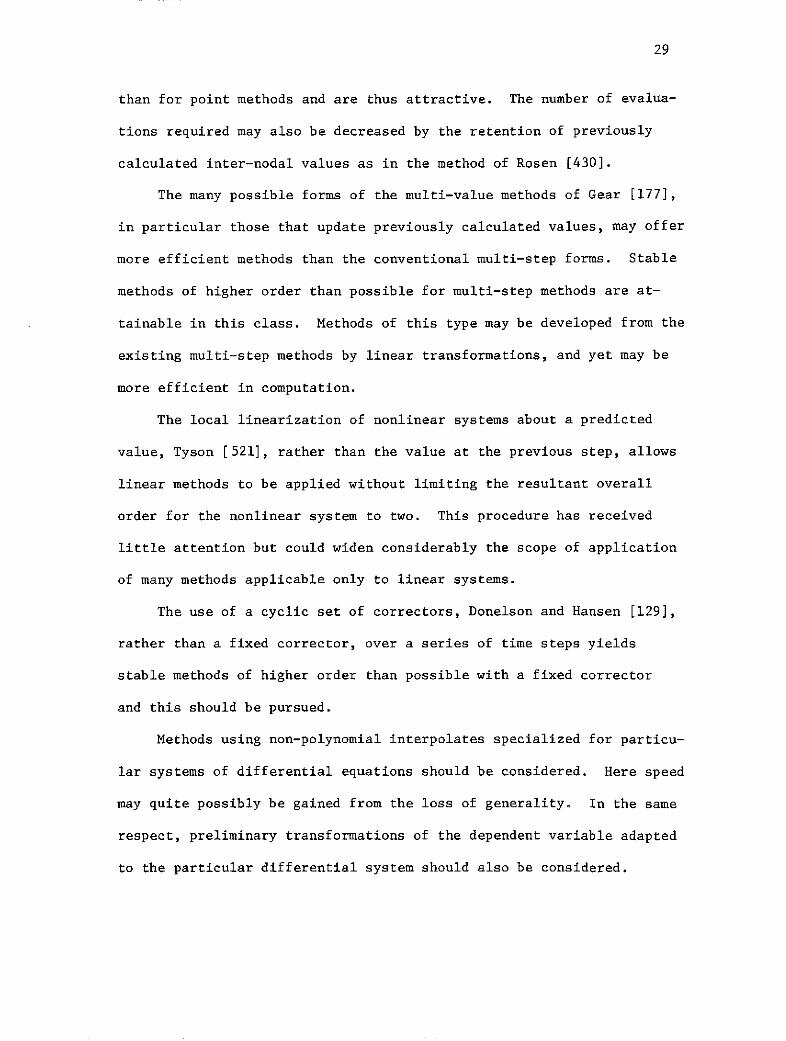
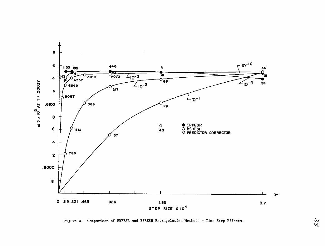
Partial results are presented in Figure 4. The best two methods
are shown, these being the Euler algorithm with polynomial function
extrapolation utilizing a reciprocal sequence for step size subdivision
(ERPESR) and the modified midpoint rule with rational function ex-
trapolation utilizing a halving sequence (BSRESH).
The accuracy of both methods is seen to be a function of step
size and tolerance between successive extrapolations. BSRESH ap-
proaches the accuracy of ERPESR but requires about 40 times as many
function evaluations at a step size of .000185 (fraction of one orbit).
At a step size of .00037 the order of the function evaluations is the

18
same but BSRESH goes unstable at higher values of time. Extrapolation
to higher tolerances increases accuracy, particularly at lower step
sizes, at the expense of increased function evaluations for both
BSRESH and ERPESH. However, there is a limit to the tolerances for
both methods below which the solution becomes unstable. And, of
course, if the tolerance is too large accuracy decreases.
ERPESH had constant accuracy over a large range of tolerances
(10 - 10 ) for step sizes between .0000231 and .000185. However,
at larger step sizes the accuracy of the solution decreased at lower
tolerances (10-4 ).
Thus the best of the extrapolation methods is ERPESR, Euler
algorithm with polynomial function extrapolation using a reciprocal
sequence to subdivide the basic step size until a tolerance between
successive extrapolation of 10 to 10- 10 is achieved. This method
gives better accuracy than the Runge-Kutta and predictor corrector
methods and takes about the same number of function evaluations. A
value of angular velocity obtained by the best of the predictor
corrector methods is shown on Figure 5 at a step size of .000185.
This value is 1.4% lower than the value obtained by ERPESR and re-
quired 40 function evaluations as compared to 41 function evaluations
-4for ERPESR when the extrapolation was carried to a tolerance of 10- 4
or 71 function evaluation for a tolerance of 10- 0 . Thus ERPESR
appears to require the same order of function evaluation as Runge-
Kutta and predictor corrector methods at a better accuracy.
19
CHAPTER IV
SURVEY OF TECHNIQUES FOR FURTHER CONSIDERATION
The numerical solution of the initial value problem
' =~f(t,y) , y(0) E . 4.1
has been approached in various ways as outlined below. As is noted,
the various classes cited are not exclusive, but overlap one another.
Quadrature Methods
One may write formally
ty(t ) = y(t ) + f r f (t, y(t)) dt 4.2
tq
In the quadrature methods, the integral in 4.2 is approximated by a
numerical quadrature expression. For instance, suppose it is desired
to calculate the numerical approximation, yn, at a series of times, tn,
n=O, 1i, 2,-**, called the nodes hereafter for convenience of notation,
these nodes not necessarily being equally spaced. Then we may approxi-
mate the integral of 4.2 by a numerical quadrature consisting of a
linear combination of nodal values and possibly also some intermediate
values at points interspersed among the nodes. The coefficients in the
linear combination and the locations of the nodes and/or the inter-nodal
points are determined by the particular type of numerical quadrature
employed. These factors are obtained directly from quadrature expres-
sions for some types of methods, but by only indirect reference to
numerical quadrature in others, the former type being that strictly
referred to as "quadrature methods" in many works.

20
If only previously calculated nodal values, and possibly the
value at the node presently under consideration, are included in the
quadrature formula, then no additional equations are required, and
the value at the node presently under consideration is determined
either explicitly or implicitly through the solution of a nonlinear
equation, depending on whether or not the value at the node under
consideration is included in the quadrature expression. Methods of
this type are also a sub-class of the linear multi-step methods dis-
cussed below.
Nesterchuk [378] gives such an implicit method involvingall previous nodal points.
If nodal points beyond the node presently under consideration are
included in the quadrature formula then an equation must be written for
each of these points, and a system of equations must then be solved
simultaneously for all the unknown nodal values involved. This type
method is also a sub-class of the block linear multi-step methods dis-
cussed below.
Day [116] gives a method of this type using Lobattoquadrature and successively higher moments of the differentialequation to supply the needed equations for all the unknownnodal values included in the block. For linear equationsthis method achieves n+l order with n function evaluationsand is reported to be superior in accuracy to some Runge-Kutta methods.
If inter-nodal points are involved, additional equations for
the values at these points must be included. If these inter-nodal
values are determined in turn by quadrature formulas, we have the
standard Runge-Kutta methods. Within this class we have explicit
methods if the expressions for the inter-nodal values involve only
values at previous inter-nodal points, semi-implicit methods if these

21
expressions involve the presently considered inter-nodal value as
well but none beyond, and implicit methods if inter-nodal values beyond
that presently considered are included. The latter types require,
respectively, the solution of one nonlinear equation at each inter-
nodal point or the simultaneous solution of a system of equations,
one for each internodal point.
The method of Hulme [253] is a generalization of this im-plicit Runge-Kutta form constructed using Gaussian quadratureto approximate the integrals involved in a Galerkin approxi-mation with the solution represented by a polynomial withineach step. This produces a piecewise continuous solutionwith essentially the same effort required by conventionalimplicit Runge-Kutta methods and the same nodal values asproduced thereby. Axelsson [13], in a general discussion ofquadrature methods, presents implicit Runge-Kutta methodsbased on Radau and Lobatto quadratures. Implicit Runge-Kutta methods are also discussed in Gourlay [194], where itis noted that certain methods stable for linear equations,i.e., with constant Jacobian matrices, may not be stablewhen the Jacobian varies as is the case with nonlinear equa-tions. The common trapezoidal method is a case in point,and a stable modification of the same order is given therefor.
Explicit Runge-Kutta methods with provision for intrinsictruncation error estimation are given in Warten [536],Sarafyan [448], and Zonneveld [553]. Haines [220] gives asemi-implicit Runge-Kutta method with the coefficients chosento increase stability and with the Jacobian matrix, requiredin such methods, evaluated by finite differences. Semi-implicit Runge-Kutta methods are also given by Allen [3].
Sarafyan [452] fits a Hermite polynomial to the inter-nodal values of an explicit embedded Runge-Kutta method toproduce a continuous approximation of order only one lessthan that of the discrete approximation. Merson [356] givesRunge-Kutta methods for which each inter-nodal value isrequired to be a good approximation of the solution at thecorresponding point. Treanor [519] uses local linearizationbefore the quadrature to develop a modification of theRunge-Kutta type. The algebraically.difficult derivationof the coefficients involved in Runge-Kutta methods is rel-egated to the computer via a program of Sarafyan and Brown[447]. Many other Runge-Kutta methods are discussed inAppendix I.

22
The more general inclusion of inter-nodal points along with nodal
points in the quadrature expression for the integral of 4.2 results
in a combination of the above types, variously referred to as multi-
step Runge-Kutta methods or hybrid methods.
Rosen [430] gives an explicit multi-step Runge-Kutta
method using at each node all the inter-nodal values used
at the previous node, with a resultant decrease in the number
of evaluations per step required for a given order.
Finally, in the manner already discussed above, the inclusion of
nodal and/or inter-nodal points beyond the node presently under con-
sideration produces block methods of the Runge-Kutta or hybrid type,
requiring simultaneous solution for all the unknown nodal and/or
inter-nodal values involved.
Block Runge-Kutta methods in which the iteration at each
node is intentionally not carried to convergence are discussed
by Rosser [433]. These methods require fewer evaluations per
step for a given order than the usual point Runge-Kutta methods.
Multi-value Methods
At each nodal point, one may write, more generally, the value of
the dependent variable, any of its derivatives, and any functions or
combinations thereof as linear combinations of these quantities at
each node and/or at inter-nodal points, and so produce the almost
all-inclusive class of multi-value methods.
Methods of this type are discussed in general in Gear [177].Methods with variable step size are discussed in regard to
stability in Tu [520].
The entire class of quadrature methods discussed above is a sub-
class of the multi-value methods for which the value of the dependent
variable, y, at only one previous nodal point is involved, and the
linear combination includes only the first derivative, y' = f (t, y).

23
The use of values of only the dependent variable and its first de-
rivative in the linear combination produces the linear multi-step methods.
These methods are explicit if only values of the derivative at previous
nodes are included, semi-implicit (commonly called implicit) if the de-
rivative at the presently-considered node is included as well but none
beyond, and implicit (commonly called "block") if nodal values beyond
that presently under consideration are included. The latter types re-
quire, respectively, the solution of a nonlinear equation at each node
or the simultaneous solution of a system of equations for all the unknown
nodal values involved. Again inter-nodal points may be included as well,
and the so-called hybrid methods developed as discussed above. The more
common types of predictor-corrector methods, in which values are "pre-
dicted" by explicit multi-value forms and then "corrected" using implicit
multi-value forms involving the predicted value as well as previously
calculated values are in this class. Additional applications of the
corrector may follow, using the most recently corrected values.
Hull and Creemer [244], in a comparison of various predictor-corrector forms, state that error, stability, and the order re-quired for a given error at least computation are less sensitiveto order with two corrector applications than with one, with nosignificant improvement thereafter. Lambert [308] shows the equiv-alence of any predictor-corrector method using a finite number ofcorrector applications to some explicit multi-step method. Thislimits the expectations for stability of predictor-correctormethods. Donelson and Hansen [129] use a set of correctors ap-plied cyclically over a set of time steps and thus achieve higher-order stable methods than are possible with the same correctorused at all steps. Order 2k-1 is thereby achieved for stable k-step methods, as opposed to the maximum order, k-l, possible withstability for methods using only a fixed corrector. The use ofvariable step size in predictor-corrector methods has been con-sidered by Van Wyk [532], and in a single-step method of themulti-step form by Richards, Lanning, and Torrey [419]. Otherpredictor-corrector methods are given in Appendix II.
Many multi-step methods have been developed in which somecoefficients are chosen to increase stability as in Krough [291],
24
with a comparison of stability plots for various methods;Crane and Lambert [96]; Nigro [383]; Rahme [406], with an at-tempt to minimize-error while maintaining stability; and Lomax[332], considering Runge-Kutta and hybrid methods as well. Amulti-step method with the coefficients chosen to fit thecharacteristic roots to some of the characteristic exponentialsof-the differential system is given by Miranker [366] for non-linear systems with local linearization, the method beingimplicit, and for linear systems by Liniger and Willoughby[323], an explicit method. Osborne [398] gives a single-stepmethod with the nodes chosen to give desired characteristicroots. Timlake [518] increases the stability of multi-stepmethods by averaging over previous steps, determining theweights from the Jacobian eigenvalues. The stability of multi-step methods has been analyzed particularly in Karim [258,256],sufficient conditions for instability being given in theformer and the effect of the predictor as well being in-cluded in the latter; Dahlquist [100-106], a series of classicpapers; and Hafner [217], giving stabtlity charts for alarge number of Runge-Kutta and hybrid methods as well.
Implicit multi-step methods particularly for stiffsystems have been giveniby Ratliff [411], giving a com-parison of several methods; Jain and Srivastava [246,247];Dill [126], a systematic search for such methods; Gelinas[182]; Dill and Gear [125], again a search; and Gear [172].Such methods achieve a particular shape of stabilityboundary suitable for stiff systems by always includingthe derivative at the present node with perhaps the deriv-atives at a few previous nodes.
Tyson [521] gives an implicit multi-step method fornonlinear systems using local linearization about a predictedvalue, rather than the previous nodal value, that achievesorder two greater than that of the predictor used. (Local
linearization is used in many methods to render nonlinearsystems tractable by methods restricted to linear systems,but such linearization about the previous nodal value re-
stricts the order to two regardless of the method used.)Boggs [30] used Broyden iteration (involving direct approxi-mation of the Jacobian inverse rather than inversion of theJacobian) with implicit multi-step methods. Block methodsare given by Daniel [109,108] and by Shampine and Watts[469]. Methods for determining the necessary set of startingvalues (a problem equivalent to the development of blockmulti-step methods) have been given in Reimer [412],Rakitskii [407], and Alonzo [4].
The addition of inter-nodal points (hybrid methods) hasbeen considered by Papian and Ball [399]; Lomax [332], whogives a method for choosing the coefficients in explicitmethods of this type to improve stability; Gragg and Stetter
25
[195]; discussing the coefficients therein for maximumorder; Gear [175]; and Hafner [217], who gives a largenumber of stability charts. Additional consideration ofmulti-step methods has been given by Spijker [492], con-sidering the question of direct application to higher-order equations or a split to a system of first-orderequations, and by Zverskina [555], using derivatives onlyat previous nodes separated by some distance from thepresent node.
Various other quantities, such as higher derivatives and divided
differences, have been included in the linear combination, and methods
using one type of quantities may be derived by transformation of
methods using another type as in Osborne [395] and Kohfeld and Thompson
[283]. Again the above-mentioned ramifications involving inter-nodal
points and/or nodal points beyond that presently under consideration
may be developed. A further modification is that values at previously
passed nodes may be subsequently changed. It is possible to derive
methods of this type that use higher derivatives or higher-order
divided differences, all of which are produced at each node from linear
combinations of the same, in lieu of values at previous nodes. In
this manner more efficient step size change can be accomplished.
In Grobner, Kohnert, Reitberger and Wanner [207] higherderivatives are included in generalizations of both implicitRunge-Kutta and multi-step type methods. Multi-value methodsinvolving higher-order derivatives are discussed in Gear[177,178]; Sloan [484]; Lewis and Stovall [321]; and Nordsieck[387], a single step form with ease of step-size change; andOsborne [395]. Kohfeld and Thompson [283] give a methodusing higher derivatives and inter-nodal points. The single-step implicit method of Urabe [522] uses second derivatives.Makinson [348] gives a single-step implicit method usinghigher derivatives, the form being specially constructed topreserve the original sparseness in the matrix solution ofthe implicit equations. Lomax [334] presents a single-stepimplicit method using second derivatives with coefficientschosen to increase stability. Ehle [132] and Davison [110]also give single-step methods using higher derivatives, andReimer [414] analyses multi-step methods using higher deriva-tives.

26
Non-Polynomial Interpolates
In the great majority of methods the linear combinations involved
in the multi-value methods, and thus in the quadrature methods, are
required to be exact when the dependent variable is a polynomial of
some degree. This restriction may be relaxed, and an even broader
spectrum of methods may be developed by requiring these linear combina-
tions to be exact for some other function, in particular for perhaps
some class of functions especially adapted to the particular differential
equation being considered.
Loscalzo and Talbot [339] use a spline function with thehigher derivatives matched at the nodes, which, while pro-ducing the same nodal values developed by a multi-stepmethod, is a single-step method and gives a piecewise con-tinuous approximation. It does, however, require differentia-tion. Byrne and Chi [45] use a spline approximation of theintergrand in a quadrature type method requiring no differentia-tian. Callender [71] uses a spline approximation spanningseveral nodes to develop a block multi-step method.
Blue and Gummel [27] and Lambert and Shaw [306] userational function approximation of matrix exponentials, theformer using coefficients chosen to increase stability andproducing thereby Pade approximates of the exponential.The latter method matches higher derivatives and thus re-quires differentiation. Roe [84] gives a multi-step methodusing a combination of a polynomial and an exponential asthe interpolate. Other non-polynomial interpolates have beenused by Shaw [475], Lambert and Shaw [303], and Pope [403],the first two being primarily of use when singularies areinvolved in the solution.
Only a relatively small number of methods of this type have
been considered, since the intention of most developments has been to
develop methods that may be applied at least fairly well to all types
of differential equations, hence the use of polynomial interpolation.
In this connection the remarks of Lomax [334] are pertinent:
"It is unlikely that 'new' combinations of linearequations that connect a function, u, and its derivative,u', at a series of reference points, equispaced or not,

27
will improve existing methods for the numerical inte-gration of general sets of coupled ordinary differentialequations..." (p. 2). "What appears to be needed arestudies of special methods designed for special methodsdesigned for special classes of equations..." (p. 6).
Iterative Methods
Methods of this class start with some approximate solution,
such as the solution of a related but simpler differential equation or
the result of any numerical method, and improve the approximation by
an iterative procedure. One such method is the Lie series method.
The extrapolation methods by which solutions with successively smaller
truncation errors are obtained by extrapolating results with succes-
sively smaller step-sizes may also be considered iterative in the sense
stated.
In reference [207] Runge-Kutta methods having error ex-pansions in even powers of the step size are developed to serveas the basis for these extrapolation methods. Lie Seriesmethods have been given by Knapp and Wanner [279,280].
Transformation Methods
In methods of this type the dependent and/or independent variable
is transformed before numerical solution in order to obtain a form with
better numerical properties. In this manner stiff systems may be
transformed into systems with smaller ranges of eigenvalues.
Lawson [313] gives a transformation of the dependentvariable which reduces the stiffness of the system, but themethod requires the use of matrix exponentials. A similartransformation of the dependent variable is used by Jain[259]. Other transformations of the dependent variable aregiven by Decell, Guseman and Lea [117], requiring evaluationof the Jacobian inverse, and by Calahan [67].
Higher-Order Equations
As is well known, any higher-order differential equation can be
broken into a set of simultaneous first-order equations to which the
28
preceding methods are applicable. Generalizations of the classes cited
follow readily, however, so that application may be made directly to
the higher-order equation if such is thought to be preferable. This
is still something of an open question.
Osborne [397] gives a quadrature method for linear higher-order equations. Day [112,113] has implicit Runge-Kutta typemethods using Gaussian and Lobatto quadrature, respectively,
for second-order equations with no first derivative. Cooper[91,93] gives a generalization of the implicit Runge-Kuttamethods to equations of any order and states that the splitinto a set of first-order equations decreases the local accuracyand increases the computation required, with little effecton the global accuracy.
The multi-value methods using higher derivatives are di-rectly applicable to higher-order equations, and Gear [177]states also that direct solution of the higher-order equationsmay be faster than that of the split system of first-orderequations. Methods of this type are also given in Gear [178,
484] and Allen [2]. Adrianova [1] found less error withoutsplitting to the first-order system. However, Spijker [503]states that round-off error is reduced by splitting into first-order equations.
Conclusions and Directions
Implicit methods in general are much more stable than explicit
methods, but may still be less efficient because of the difficulty
of the solution of the system of simultaneous equations that is
required at each time step. The key to the use of the more stable im-
plicit schemes is thus the iterative solution of this system, and ef-
fort should be directed toward the development of faster and more ap-
propriate iterative schemes for use in these methods. There are, of
course, a great many general iterative schemes that have never been
applied in implicit numerical solutions of ordinary differential
equations.
Block methods with a set number of iterations, such as that of
Rosser [432], can achieve a given order with fewer evaluations per step
29
than for point methods and are thus attractive. The number of evalua-
tions required may also be decreased by the retention of previously
calculated inter-nodal values as in the method of Rosen [430].
The many possible forms of the multi-value methods of Gear [177],
in particular those that update previously calculated values, may offer
more efficient methods than the conventional multi-step forms. Stable
methods of higher order than possible for multi-step methods are at-
tainable in this class. Methods of this type may be developed from the
existing multi-step methods by linear transformations, and yet may be
more efficient in computation.
The local linearization of nonlinear systems about a predicted
value, Tyson [521], rather than the value at the previous step, allows
linear methods to be applied without limiting the resultant overall
order for the nonlinear system to two. This procedure has received
little attention but could widen considerably the scope of application
of many methods applicable only to linear systems.
The use of a cyclic set of correctors, Donelson and Hansen [129],
rather than a fixed corrector, over a series of time steps yields
stable methods of higher order than possible with a fixed corrector
and this should be pursued.
Methods using non-polynomial interpolates specialized for particu-
lar systems of differential equations should be considered. Here speed
may quite possibly be gained from the loss of generality. In the same
respect, preliminary transformations of the dependent variable adapted
to the particular differential system should also be considered.

30
TABLE I
EQ. RMS TE x 10-10
IN
Explicit Runge-Kutta AP- T ET = (RMS TE/2P+1-2)(V/h) x 10x
RKE(p,V) DIX M1 E hE
-1.001 .0005 .00025 .000125 .0000625 .00003125 .000015625
ai A.26 1.578x0 1.686x03 1.05x10² 6.325 2.683 0
4.206-4 8.99-5 1.10-5 1.349-6 1.145-6
A 1.578x10 1.686x10³ 1.05x10²
6.325 3.578 0ill(4,4) A.-25 4--------- - - -- - ---- -- --- --- ---------I(4,4) A.25 4.206-4 8.99-5 1.12-5 1.349-6 1.527-6
S1.565x104 1.58x10³ 1.04x10² 6.325 2.951 0alston(4,4) A.21 4 -- 4.173-4 8.43-5 1.11-5 1.349-6 1.259-6
S-1.006x10⁴ 3.95X10² 2.24x101 0-ystrom(5,6) A.34 6---- ----- --1.95x10⁻⁴ 1.53-5 1.73-6
Butcher(5,6) 3.107x10³ 1.789 0
gewton-Cotes Quadrature A.386.013-5 2.07-6 1.39-7
awson(5,6) .973x108
4.49x10³ 1.18x10²
3.578 0A.42 6Newton-Cotes Quadrature A876 8.689-5 4.58-6 2.77-7
4.64x03 1.03xlO2
3.130 0Fehlberg(5,6) A.49 6 ---.. 6A 3 1.03x 3.130 0
8.98-5 4.0-6 2.423-
Luther(5,6) 3.65x10 9.04x10² 2.683x101 0Newton-Cotes Quadrature A.35 6 .------ ----- -------
Newton-Cotes Quadrature 7.05-4 3.50-5 2.08-6
Luther(5,6) 2.88x10⁴ 6.90x10² 2.06x01 0
Gauss Quadrature A.43 6 5.32-4 2.67-5 -- 1.59-6 -- ---
Luther(5,6) 1.02x10³
2.70x10² 8.05 0Radau Quadrature A.44 6 ---------- x-!2 ---. --..... . -Radau Quadrature 1.976-4 1.05-5 6.234-7
Luther(5,6) 1.02x10³
2.70x10² 8.05 0Lobatto Quadrature A.45 6 1.976-4 1.05-5 - -.234-7
Shank(5 A.47 9.898xl011 1.057x10³
2.72xl02 1.297x10 0N-5 7.982+3 1.64-4 8.78-6 8.37-7
11 4 3 2Shanks(5,5) .692x10 1.375x10 1.151xlO 1.127x02 0N--100 A.47 5 -- - ------ -----------------------
100 .817+3 2.22-4 3.71-5 7.27-6
Modified Shanks(5,4) 2.64x10 4.20x10³ 4.03x10² 0N-100 A.48 4 3.41- .20- 4.03N-a 3.41-4-- 1.08-4 2.08-S
Butcher(6,7) 7Butcher(6,7) K 1.046x10 1.19x10 1.789 1.265 1.789 0ewton-Cotes Quadrature A.57 1.16-4 2.63-6 7.947-8 1.124-7 3.18-7
1.233x10¹² 2.52xl03 3.54x101 .894 .6325 2.683 0S a k (6,6) A.67 6-- - - - - - - - - - - - - - - - - - - --- - - - -Shanks(6,6) A.67 6 .872+3 2.4-5 6.75-7 3.407-8 4.819-8 4.04-7
Sarafyan(7,10) .575s103 3.64+1 .949 1.789 0 - -wton-Cotes Quadrature A.68 10 .80-5 2.87-7 1.49-8 5.635-8
5.18x10² 4.427 .894 0S a k (7.7) A.73 7 - - - - - - - - - - - - - - - - - - - - - - - -:- - - - -Shanks(7,7) A.73 7 2.85-6 4.88-8 1.971-8
.108x104 9.41x101 .949 1.342 2.530 5.367 0Curtis(8,11) A.75 11 -- -- ------ ----- ---------urti(8,11) A.75 11 .704-5 . 4.06-7 8.18-9 2.315-8 8.728-8 3.704.-7
.949x104 9.21xl01 .949 1.789 2.530 5.367 0Shanks(8,10) A.77 10 781-5 3.62-7 7.44-9 2.806-8 7.931-8 3.368-7
The signed number following each entry indicates multiplication by the corresponding power of 10.
31
TABLE II-10EQ. VRMS TE 10 -
EQ. V
MULTISTEP IN T ET = (RMS TE/2p1-2)(V/h) 10xMETHOD AP- I
PEN- h -DIX
.0005 .00025 .000125 .0000625 .00003125
AB(3,3) 31 2 1.54x10⁴ 1.955x10³ 0M(3,2)(PECE) 55 8.80-6 2.23-6
A(3 3) 31 2 X 6.75x103 1.185x10³ 0, 56 1.80-6 6.32-7
AB(3,3) 31 X 7.77x103 1.07x10³ 0, 3)--C--- 56 1.035-6 2.85-7
C_(44) 4 X - 4.24x10² 40.6 0
M43)(PCE) 56 2 2.26-7 -- 4.3--
Butcher Hybrid 1 X 1.71x103 57.2 0fifth order 3 3.30-7 2.22-8
CK(44) 4 X 4.12x103 1.55x10² 31.7 0Wesson(5,5)(PECE) 73 5.3-7 4.0-8 1.5-
AB(4.4 32 X 2.57x103 6.09x10² 0
(6,5)(rECE) 58 2 6-7 1.73-7
ro(44) 25 2.61x10³ 3.46x10² 0
65PECE 58 2 5.23-7 9.85-8
(4,4) 32 1 1.40x10⁴ 2.46x10³ 0
(6,5)( 58 1 1. 3.53-7
(44) 25 X 1.40x104 2.46x10³ 0,5 ) 58 1.40-6 3.53-7
K(4,4) 4 X 1.537x103 82.6 0A W(,5?i 58 29.77-- 1.05-8
1-, 4 1 4.81x10 3 3.13x10² 06 -5 58 1.55-7 1.99-8
AB(8 8) 36 X X 2.1x103 7.9x10² 08!,F C-ET 60 6.58-8 .97-8
4 4 2 X 85. 22.8 07"E-7 60 2.0-9 1.3-10
CK(44 4 X - 96.5 24. 0es ii ETn -'2 74 .3-9 1.50-10

32
o
-C.o I I
o
x-
0
o
'0.0o0 n. ' 0.00 O.2 I 0.16 O. 0 O.2 0.28 0. 3. .?E ;.
TIME
figure 1. W 3 and q3 up to T = .25 (quarter of an orbit).

33
eo F 4V
c, -H
> 3-H
C'J*.
I I
'" 'i\ \l V
J, / ..
C.-:
Ci
i i
- i
I'0. Q 0.05 0.10 0.15 0.20 0.25 0.30 0.35 40TIME X10 - 1
Figure 2. Errors in W and q versus time, up to T .04.Figure 2. Errors in W 3 and q3versus time, up to T =.04.

34
01
cMULTIPLE OF C TME STEP
RK-RALSTON(, 14) OPTIMISED FOR T.E. ICLAIMED TO BE BETTER THAN GILL(4.41)
COMPARISION FOR TRUNCATION ERROR IBASED ON SMALLEST
STEP-SIZE AS THE ACCURATE SOLUTIONI
6 RUNS MADE FROM H-.000015625 TO H=.0005 , DOUBLING THE H EACH TIME
TILL THE METHOD GOES UNSTABLE, THE LAST RUN IS THE LAST STABLE H USABLE
COMPARISION RUN TO T-.04. THIS INTERVAL INCLUDES A TIME OF HIGH
OSCILLmTION AND R TIME OF STRAIGHT DECAT. OSCILLATIONS !TOP AT ABOUT
T=.02. T-.04 CORRESPONDS TO NSTEPS2560 FOR HM.000015625
Figure 3. RMS error in W3 versus step size.
TILTE E~O OSUNTBE.'H LS UNI nELS SRL 3URL
6 -1100 561 440 71 10-10
4 143 4 3091 2073 L 10-3 93o 6369 2 10-4 as
o 2
8097- 10-
.6100 - 29
x 8
a1 O 0 ERPESR6 561 40 O BSRESH
0 PREDICTOR CORRECTOR57
4
2 785
.6000
8
0 .115 .231 .463 .926 1.85 3.7
STEP SIZE X 10 4
Figure 4. Comparison of ERPESR and BSRESH Extrapolation Methods - Time Step Effects.

BSRESH.6154 -ERPESR
H=.00037
.615H=.0000116
.6152 - = - 0 \0 X.00009- --- ..96 4 H=000023 \
0 \ \I\ o\
o .6150 --- O --------------------- \0 H =:.000185o
0 \\ \'
.6148 \ \ \ .610
.6146
.6144 I
v .605
1-12 1-10 1O IO" 10- 103 10 2 10.
TOLERANCE BETWEEN SUCESSIVE EXTRAPOLATIONS
Figure 5. Comparison of ERPESR and BSRESH Extrapolation Methods - Tolerance Effects.

BIBLIOGRAPHY
1. Adrianova, L., "Comparison of Precision of Numerical Integration ofSecond Order Differential Equations with Their CorrespondingSystems of First Order Differential Equations," Diff. Eq. 3,788 (1967).
2-. Allen, R., "A New Method of Solving Second-Order DifferentialEquations When the First Derivative Is Present," Comp. J. 8,392 (1965-66).
3. Allen, R., "Numerically Stable Explicit Integration TechniquesUsing a Linearized Runge-Kutta Extension," Info. Sci. Rept.39, Boeing Scientific Research Lab. (1969).
4. Alonzo, R., "A Starting Method for the Three-Point Adams Predictor-Corrector Method," J. Assoc. Comp. Mach. 7 (1960).
5. Anderson, N., Ball, R., & Voss, J., "A Numerical Method for Solv-ing Control Differential Equations on Digital Computers,"J. Assoc. Comp. Mach. 7, 61 (1960).
6. Anderson, W., "The Solution of Simultaneous Ordinary DifferentialEquations Using a General Purpose Digital Computer," Comm.ACM 3, 357 (1960).
7. Andrus, J., "Integration of Control Equations & the Problem ofSmall Time Constants," NASA Tech. Note D-3907 (1967).
8. Ansorge, R., "Zur Struktur gewisser Konvergenzkriterien bei dernumerischen Losung von Anfangswertaufgaben," Num. Math. 6,224 (1964).
9. Ansorge, R., "Konvergenz von Mehrschrittverfahren zur LosungHalblinearer Anfangswertaufgaben," Num. Math. 10, 209 (1967).
10. Ansorge, R., & Tornig, W., "Zur Stabilitat des NystromschenVerfahrens," ZAMM 40, 568 (1960).
11. Antosiewicz, H. & Gautschi, W., "Numerical Methods in OrdinaryDifferential Equations," A Survey of Numerical Analysis,Editor, J. Todd, McGraw-Hill, New York 314 (1962).
12. Aronson, D., "The Stability of Finite Difference Approximation toSecond Order Linear Parabolic Differential Equations," DukeMath. J. 30, 117 (1963).
13. Axelesson, 0., "A Class of A-Stable Methods," BIT 9, 185 (1969).
14. Axelsson, 0., "Global Integration of Differential EquationsThrough Lobatto Quadrature," BIT 4, 69 (1964).

38
15. Ballester, C. & Pereyrn, V., "On the Construction of DiscreteApproximation to Linear Differential Expressions," Math.Comp. 21, 297 (1967).
16. Bard, A., Ceschino, F., Kunttmann, J., Launrent, P., "Formules deBase de le Methode de Runge-Kutta," Chiffres 4, 31 (1961).
17. Baron, W., "Stabilitatsgebiete fur Predictor-Corrector-Vergahren,"Master's Thesis TH Wien (1968).
18. Baxter, D., "The Digital Simulation of Transfer Functions," Nat.Res. Council of Canada Mech. Eng. Report MK-13 (1964).
19. Baxter, D., "Digital Simulation Using Approximate Methods," Nat.Res. Council of Canada Mech. Eng. Report MK-15 (1965).
20. Baxter, D., "The Step Response of Digital Simulation," Nat. Res.Council of Canada Mech. Eng. Report MK-14 (1965).
21. Bellman, R. & Richardson, J., "On Some Questions Arising in theApproximate Solution of Nonlinear Differential Equations,"guar. Appl. Math. 20, 333 (1963).
22. Benyon, P., "Comments on Giese's Paper, State Variable DifferenceMethods for Digital Simulation," Sim. 8, 270 (1967).
23. Benyon, P., "A Review of Numerical Methods for Digital Simulation,"Sim. 11, 219 (1968).
24. Birkhoff, G., "Numerical Integration of Reactor DynamicsEquations," Symposium on the Numerical Solution of NonlinearDifferential Equations, Math. Res. Center, Univ. ofWisconsin, Madison (1966).
25. Bjurel, G., "Preliminary Report on Modified Linear MultistepMethods for a Class of Stiff Ordinary Differential Equations,"Dept. of Info. Processing, The Royal Institute of Technology,Stockholm, Report #NA 69.02 (1969).
26. Bjurel, G., Dahlquist, B., Lindberg, B., Linde, S., & Oden, L.,"Survey of Stiff Ordinary Differential Equations," Dept. ofInformation Processing, Royal Institute of Technology,Stockholm, Report #NA 70.11 (1970).
27. Blue, J., & Gummel, H., "Rational Approximations to MatrixExponential for Systems of Stiff Differential Equations,"J. Comp. Phy. 5, 70 (1970).
28. Blum, E., "A Formal System for Differentiation," J. Assoc. Comp.Mach. 13, 495 (1966).

39
29. Blum, E., "A Modification of the Runge-Kutta Fourth-Order Method,"Math. Comn. 16, 176 (1962).
30. Boggs, P., "The Solution of Nonlinear Systems of Equations byA-Stable Integration Techniques," SIAM J. Num. Anal. 8, 767(1971).
31. Borshch, Yu., "On a Matrix Algorithm for Solving Linear Differen-tial Equations and sets of Such Equations," U.S.S.R. Comp.Math. & Math. Phy. 7, 231 (1967).
32. Bramble, J., "Error Estimates for Difference Methods in ForcedVibration Problems," SIAM J. Num. Anal. 3, 1 (1966).
33. Brandin, E., "The Mathematics of Continuous System Simulation,"AFIPS Conference Proceedings, 33 (1966).
34. Braun, J. & Moore, R., "Solution of Differential Equations,"Math. Res. Center, Report #901 (1968).
35. Brayton, R., "Necessary & Sufficient Conditions for BoundedGlobal Stability of Certain Nonlinear Systems," Quar. Appl.Math. 6, 237 (1971).
36. Brayton, R., Gustavson, F., & Liniger, W., "A Numerical Analysisof the Transient Behavior of a Transistor Circuit," IBM J.Res. & Dev. 10, 292 (1966).
37. Brayton, R., Gustavson, F., Hacktel, R., "A New Efficient Algorithmfor Solving Differential Algebraic Systems Using ImplicitBackground Difference Formulas," Proc. IEEE 60, 98 (1972).
38. Brennan, R. & Linbarger, R., "A Survey of Digital Simulation;Digital Analog Simulator Programs," Sim. 3, 22 (1964).
39. Brock, P. & Murrary, F., "The Use of Exponential Sums in Stepby Step Integration," MTAC 6, 63 (1952).
40. Brooks, J. & Pope, D., "Asymptotic Error Estimates & The NumericalSolution of the Equations of Orbital Motion," SIAM J. Num.Anal. 4, 446 (1967).
41. Brown, R., Riley, J., & Bennett, M., "Stability Properties ofAdams-Moulton Type Methods," Math. Comp. 19, 90 (1965).
42. Brunner, H., "Marginal Stability & Stabilization in the NumericalIntegration of Ordinary Differential Equations," Math. Comp.24, 635 (1970).
43. Brunner, H., "Stabilization of Optimal Difference Operations,"ZAMP 18, 438 (1967).
40
44. Brush, D., et al., "Solution of Ordinary Differential EquationsUsing Two 'Off-Step' Points," J. Assoc. Comp. Mach. 14, 769(1967).
45. Bryne, G. & Chi, D., "Linear Multistep Based on G-Splines," SIAMJ. Num. Anal. 9, 316 (1972).
46. Bulirsch, R. & Stoer, J., "Fehlerabschatzungen und Extrapolationmit Rationalen Funktionen bei Verfahren von Richardson-Typus," Num. Math. 6, 413 (1964).
47. Bulirsch, R. & Stoer, J., "Numerical Treatment of OrdinaryDifferential Equations by Extrapolation Methods," Num. Math.8, 1 (1966).
48. Bulirsch, R. & Stoer, J., "Asympotic Upper and Lower Bounds forResults of Extrapolation Methods," Num. Math. 8, 93 (1966).
49. Butcher, J., "An Algebraic Theory of Integration Methods," Math.Comp. 26, 79 (1972).
50. Butcher, J., "A Convergence Criterion for a Class of IntegrationMethods," Math. Comp. 26, 107 (1972).
51. Butcher, J., "A Multistep Generalization of Runge-Kutta Methodswith Four or Five Stages," J. Assoc. Comp. Mach. 14, 84(1967).
52. Butcher, J., "A Modified Multistep Method for the NumericalIntegration of Ordinary Differential Equations," J. Assoc.Comp. Mach. 12, 124 (1965).
53. Butcher, J., "Coefficients for the Study of Runge-Kutta IntegrationProcesses," J. Aus. Math. Soc. 3, 185 (1963).
54. Butcher, J., "Implicit Runge-Kutta Processes," Math. Comp. 18,50 (1964).
55. Butcher, J., "Integration Processes Based on Radau QuadratureFormulas," Math. Comp. 18, 233 (1964).
56. Butcher, J., "On Attainable Order of Runge-Kutta Methods," Math.Comp. 19, 408 (1965).
57. Butcher, J., "On the Convergence of Numerical Solutions toOrdinary Differential Equations," Math. Comp. 20, 1 (1966).
58. Butcher, J., "On the Integration Processes of A. Huta," J. Aus.Math. Soc. 3, 203 (1963).
59. Butcher, J., "On Runge-Kutta Processes of High Order," J. Aus.Math. Soc. 4, 179 (1964).
41
60. Butcher, J., "The Effective Order of Runge-Kutta Methods,"Conference on the Numerical Solutions of DifferentialEquations, Lecture Notes in Math. #109, Springer-Verlag,Berlin, 133 (1969).
61. Butcher, J., "On the Convergence of Numerical Solutions toOrdinary Differential Equations," Math. Comp. 20, 1 (1966).
62. Byrne, G. & Lambert, R., "Pseudo-Runge-Kutta Methods InvolvingTwo Points," J. Assoc. Comp. Mach. 13, 114 (1966).
63. Byrne, G., "Pseudo-Runge-Kutta Involving Two Points,"Ph.D. Thesis, Iowa State University (1963).
64. Byrne, G., "Parameters for Pseudo-Runge-Kutta Methods," Comm.ACM 10, 102 (1967).
65. Calahan, D., "Efficient Numerical Analysis of Nonlinear Circuits,"Proc. 6th Annual Allerton Conference on Circuit & SystemTheory, Univ. of Illinois, Urbana 321 (1968).
66. Calahan, D. & Gear, C., "An Ill-Conditioning Problem withImplicit Integration," Proc. IEEE 57, 1775 (1969).
67. Calahan, D., "Numerical Consideration in the Transient Analysisand Optimal Design of Nonlinear Circuits," Digest Recordof Joint Conference on Mathematical and Computer Aids toDesign, ACM/SIAM/IEEE, Anaheim, California 129 (1969).
68. Calahan, D., "Numerical Solutions of Linear Systems With WidelySeparated Time Constants," Proc. IEEE 55, 2016 (1967).
69. Calahan, D. & Abbott, N., "Stability Analysis of NumericalIntegration," Proc. 10th Midwest Symp. on Circuit Theory,Purdue Univ., Lafayette, Indiana (1967).
70. Calahan, D., "A Stable Accurate Method of Numerical Integrationfor Nonlinear Systems," Proc. IEEE 56, 744 (1968).
71. Callender, E., "Single Step Methods and Low Order Splines forSolutions of Ordinary Differential Equations, SIAM J. Num.Anal. 8, 61 (1971).
72. Carr, J., "Error Bounds for the Runge-Kutta Single-StepIntegration Process," J. Assoc. Comp. Mach. 5, 39 (1958).
73. Case, J., "A Note on the Stability of Predictor-CorrectorTechniques," Math. Comp. 23, 741 (1969).
74. Casity, C., "Solutions of the Fifth Order Runge-Kutta Equations,"SIAM J. Num. Anal.3, 598 (1966).
42
75. Cassity, C., "The Complete Solution of the Fifth Order Runge-KuttaEquations," SIAM J. Num. Anal. 6, 432 (1969).
76. Certaine, J., "The Solution of Ordinary Differential Equationswith Large Time Constants," Mathematical Methods for Digital
Computers, Ralston & Wilf, ed., Wiley, New York 128 (1960).
77. Ceschino, F., "Modifications de la Longueur du pas dan L'ingrationNumerique par les Methods a pas Lies," Chiffres 2, 101 (1961).
78. Ceschino, F., "Une Methode de Mise en Oeucre des Formulesd'Obrechkoff pour L'integration des Equations Differen-tielles," Chiffres 2, 49 (1961B).
79. Chai, A., "Error Estimate of a Fourth-Order Runge-Kutta Methodwith Only One Initial Derivative Evaluation," AFIPS Conf.Proc. 32, 467 (1968).
80. Chai, A., "A Modified Runge-Kutta Method," Sim. 10, 221 (1968).
81. Chi, D., "Linear Multistep Based on G-Splines," Doctorial ThesisUniversity of Pittsburgh (1970).
82. Chase, P., "Stability Properties of Predictor-Corrector Methodsfor Ordinary Differential Equations," J. Assoc. Comp. Mach.9, 457 (1962).
83. Christiansen, J., "Numerical Solution of Ordinary SimultaneousDifferential Equations of the First Order Using a Methodfor Automatic Step Change," Num. Math. 14, 317 (1970).
84. Clancey, J. & Fineberg, M.,"Digital Simulation Languages, ACritique and a Guide," AFIPS Conf. Proc. 27 (1965).
85. Clark, N., "Program Description for Library Subroutine ANL D250DIFSUB," Argonne National Lab., Argonne, Ill. (1966)z
86. Clark, N., "A Study of Some Numerical Methods for the Integrationof Systems of First-Order Ordinary Differential Equations,"Argonne National Lab. Report, ANL-7428 (1968).
87. Clenshaw, C. & Curtiss, A., "A Method for Numerical Integrationon an Automatic Computer," Num. Math. 2, 197 (1960).
88. Clenshaw, C., "The Numerical Solution of Linear DifferentialEquations in Chebyshev Series," PICC Symposium, Rome, onDifferential & Integral Equations, Birkhauser, Basel 222(1960).
89. Cohen, C. & Hubbard, E., "An Algorithm Applicable to NumericalIntegration of Orbits in Multiple Revolution Steps,"Astron. J. 65, 454 (1960).

43
90. Cooke, C., "On Stiffly Stable Implicit Linear Multistep Methods,"SIAM J. Num. Anal. 9, 29 (1972).
91. Cooper, G., "A Class of Single-Step Methods for Systems of Non-linear Differential Equations," Math. Comp. 21, 597 (1967).
92. Cooper, G., "Error Bounds for Numerical Solutions of OrdinaryDifferential Equations," Num. Math. 18, 162 (1971).
93. Cooper, G., "Interpolation & Quadrature Methods for OrdinaryDifferential Equations," Math. Comp. 22, 69 (1968).
94. Cooper, G. & Gal, E., "Single-Step Methods for Linear DifferentialEquations," Num. Math. 10, 307 (1967).
95. Crane, R. & Klopfenstein, R., "A Predictor-Corrector Algorithmwith an Increased Range of Absolute Stability," J. Assoc.Comp. Mach. 12, 227 (1965).
96. Crane, R. & Lambert, R., "Stability of a Generalized CorrectorFormula," J. Assoc. Comp. Mach. 9, 104 (1962).
97. Cullum, J., "Numerical Differentiation and Regularization," SIAMJ. Num. Anal. 8, 254 (1971).
98. Curtis, A., "An Eight Order Runge-Kutta Process with ElevenFunction Evaluations per Step," Num. Math. 16, 268 (1970).
99. Curtiss, C. & Hirachfelder, J., "Integration of Stiff Equations,"Proc. Nat. Acad. Sci. U.S.A. 38, 235 (1952).
100. Dahlquist, G., "Convergence and Stability in the NumericalIntegration of Ordinary Differential Equations," Math.Scand. 4, 33 (1956).
101. Dahlquist, G., "A Numerical Method for Some Ordinary DifferentialEquations with Large Lipschitz Constants," Proc. IFIPCongress, Edinburgh (1968).
102. Dahlquist, G., "On Rigorous Error Bounds in the Numerical Solutionof Ordinary Differential Equations," The Numerical Solutionof Nonlinear Differential Equations, ed. D. Greenspan, Wiley,New York 89 (1966).
103. Dahlquist, G., "Stability and Error Bounds in the NumericalIntegration of Ordinary Differential Equations," Kungl.Tekniska Hogskolans Handlingar 130 (1959).
104. Dahlquist, G., "Stability Questions for Some Numerical Methodsfor Ordinary Differential Equations," ExperimentalArithmetic High Speed Computing & Mathematics, Proc. ofSymposium on Applied Math. XV, Amer. Math. Soc., Providence(1963).

44
105. Dahlquist, G., "Stability Questions for Some -Numerical Methodsfor Ordinary Differential Equations," AMA Proc., SymposiaAppl. Math. 15, 147 (1963).
106. Dahlquist, G., "A Special Stability Problem for Linear MultistepMethods," BIT 3, 27 (1963).
107. Danchick, R., "Further Results on Generalized Predictor-Corrector Methods," J. Comp. & Sys. Sci. 2, 203 (1968).
108. Daniel, J., Pereyra, W. & Shumaker,L., "Iterated Deferred Correc-tions for Initial Value Problems," Math. Res. Cntr. Report# 808 (1967).
109. Daniel, J., "Nonlinear Equations Arising in Deferred Correctionof Initial Value Problems," Math. Res. Cntr. Report #818(1967).
110. Davison, E., "A High Order Crank-Nicjolson Technique for SolvingDifferential Equations," Comp. J. 10, 195 (1967).
111. Davison, E., "The Numerical Solution of Large Systems of LinearDifferential Equations," AIChE J. 14, 46 (1968).
112. Day, J., "A One-Step Method for the Numerical Integration of theDifferential Equations y" = f (x) y + g (x)," Comp. J. 7,314 (1965).
113. Day, J., "A One-Step Method for the Numerical Solution of SecondOrder Linear Ordinary Differential Equations," Math. Comp.18, 664 (1964).
114. Day, J., "A Runge-Lutta Method for the Numerical Integrationfor the Differential Equation y" = f(x,y)," ZAMM 5, 354(1965).
115. Day, J., "A Runge-Kutta Method for the Numerical Solution of theGoursat Problem in Hyperbolic Partial Differential Equations,"Comp. J. 9, 81 (1966).
116. Day, J., "Quadrature Methods for Arbitrary Order for SolvingLinear Ordinary Differential Equations," BIT 6, 181 (1966).
117. Decell, H., et al., "Concerning the Numerical Solution ofDifferential Equations," Math. of Comp. 20, 431 (1966).
118. Dejon, B., "Numerical Stability of Difference Equations withMatrix Coefficients," SIAM J. Num. Anal. 4, 119 (1967).
119. Dejon, B., "Stronger Than Uniform Convergence of MultistepDifference Methods," Num. Math. 8, 29 (1966).
45
120. Dejon, B., "Addendum to Stronger Than Uniform Convergence Multi-step Difference Methods," Num. Math. 9, 268 (1966).
121. Dennis, S., "The Numerical Integration of Ordinary DifferentialEquations Possesing Exponential Type Solutions," Proc.Cambridge Philos. Soc. 56, 240 (1960).
122. Dennis, S., "Step By Step Integration of Ordinary DifferentialEquations," Applied Math. Quart. 20, 359 (1962).
123. Descloux, J., "A Note on a Paper by A. Nordsieck," Dept. ofComp. Sci. Report 131, Ill. (1963).
124. Devyotko, V., "On a 2-Sided Approximation for the NumericalIntegration of Ordinary Differential Equations," U.S.S.R.Comp. Math. & Math. Phys. 3, 336 (1963).
125. Dill, C., & Gear, C., "A Graphical Search for Stiffly StableMethods for Ordinary Differential Equations," J. Assoc.Co. Mach. 18, 75 (1971).
126. Dill, C., "A Computer Graphic Technique for Finding NumericalMethods for Ordinary Differential Equations," Dept. ofComputer Sci. Rept. 295, University of Illinois (1969).
127. Distefano, G., "Stability of Numerical Integration Techniques,"AIChE J. 11, 946 (1968).
128. Dolgopolova, T., & Ivanov, V., "On Numerical Differentation,"U.S.S.R. Comp. Math. & Math. Phys. 4, 174 (1966).
129. Donelson, J., & Hansen, E., "Cyclic Composite Multistep Pre-doctor-Corrector Methods," SIAM J. Num. Anal. 8, 137 (1971).
130. Durham, H., et al., "Study of Methods for Numerical Solution ofOrdinary Differential Equations," NASA CR 57430 (1964).
131. Dyer, J., "Generalized Multistep Methods in Satellite OrbitComputation," J. Assoc. Comp. Mach. 15, 712 (1968).
132. Ehle, B., "High Order A-Stable Methods for the NumericalSolution of Systems of Differential Equations," BIT 8, 276(1968).
133. Ehle, B., "On Pade Approximations to the Exponential Functionsand A-Stable Methods for the Numerical Solution of InitialValue Problems," Res. Rept. CSRR 2010, University ofWaterloo (1969).
134. Eisenpress, H., & Bomberault, A., "Efficient Symbolic Differen-tiation Using PL/1-FORMAC," IBM New York Scientific CenterReport 320-29561 (1968).
46
135. El-Sherif, H., "Implicit Implementation of the Weighted BackwardEuler Formula," IBM J. Res. Develop. 6, 336 (1968).
136. El-Sherif, H., "Solution of Electromechanical Systems Using AWeighted Backward Euler Formula," Proc. First Annual ASILOMARConference on Circuits & Systems, 11 (1967).
137. Emanuel, G., "The Wilf Stability Criterion for Numerical Integrat-ion," J. Assoc. Comp. Mach. 10, 557 (1963).
138. Emanuel, G., "Numerical Analysis of Stiff Equations," SSD-TDR-63-380, Aerospace Corp., El Segundo, California (1964).
139. Emanuel, G., "Problems Underlying the Numerical Integration fokthe Chemical & Vibrational Rate Equations in a Near-Equili-brium Flow," AEDC-TDR-63-82, Aerospace Corp., El Segundo,California (1963).
140. Engeli, M., "Achievements & Problems in Formula Manipulation,"Information Processing 68, ed. A. J. H. Morrell, NorthHolland Publishing Co., Amsterdam 24 (1969).
141. England, R., "Error Estimates for Runge-Kutta Type Solutions toSystems Of Ordinary Differential Equations," Comp. J. 12,166 (1969).
142. England, R., "Automatic Methods for Solving Systems of OrdinaryDifferential Equations," Thesis, University of Liverpool(1967).
143. Falbi, P. & Groome, G., "Stability of Difference Approximationsto Differential Equations," J. Diff. Eq. 13, 48 (1973).
144. Fedenko, N., "A Remark on the Instability of Certain NumericalSolution Schemes for the Cauchy Problem," Instute of Math.AS BSST 11, 172 (1964).
145. Fehlberg, E., "Classical Fifth-, Sixth-, Seventh-, & Eight-Order Runge-Kutta Formulas With Stepsize Control," NASA Tech-nical Report, NASA TR R-287 (1968).
146. Fehlberg, E., "Eine Methode zur Fehlerverkleinerung beim Runge-Kutta Verfahren," ZAMM 38, 421 (1958).
147. Fehleberg, E., "Klassische Runge-Kutta-Formeln vierter undniedreigerer Ordung Mit Schrittwein-Kontrolle und ihreAnwendung auf Warmeleitungsprobleme," Computing (Arch.Elektron, Rechnen), 6, 61 (1970).
148. Fehlberg, E., "Low-Order Classical Runge-Kutta Formulas WithStepsize Control," NASA Technical Report, M-256 (1969).
47
149. Fehlberg, E., "Neue Genauere Runge-Kutta Formeln fur Differen-tialgleichungen n-ter Ordung," ZAMM 40, 449 (1960).
150. Fehlberg, E., "New High-Order Runge-Kutta Formulas with StepSize Control for Systems of First- and Second-Order Differen-tial Equations," Presented by S. Filippi at the Meeting of theGAMM in Giessen, Germany April (1964).
151. Fehlberg, E., "New High-Order Runge-Kutta Formulas with an Arbit-rarily Small Truncation Error," ZAMM 45 (1965).
152. Fehlberg, E., "Numerically Stable Interpolation Formulas WithFavorable Error Propagation for First & Second Order Diffe-
rential Equations," NASA TN D-599 (1961).
153. Fehlberg, E., "Runge-Kutta Type Formulas of High-Order Accuracy& Their Application to the Numerical Integration of theRestricted Problem of Three Bodies," Presented at the Col-loque Interantianal des Techniques de Calcul Analogique etNumerique in Aeronaitique in Liege, Belgium, Sept. (1963).
154. Feldstein, M., & Stetter, H., "Simplified Predictor-CorrectorMethods," Assoc. Comput. Mach. National Conference (1963).
155. Ferguson, R., & Orlow, T., "FNOL 3, A Computer Program to SolveOrdinary Differential Equations," Naval Ordance Lab, WhiteOak, Silver Spring, Maryland, March (1971).
156. Filippi, S., "Contribution To The Implicit Runge-Kutta Process,"Elektronische Datenverarbeitung 10, 113 (1968).
157. Filippi, S., & Glasmacher, W., "New Results On Applying TheRunge-Kutta Processes With The Aid of Nonnumerical Programs,"Elektronische Datenverarbeitung 10, 16 (1968).
158. Forrington, C., "Extensions of the Predictor-Corrector Method forthe Solution of Systems of Ordinary Differential Equations."Comp. J. 4, 80 (1961-1962).
159. Forrington, C., "The Numerical Solution of System of DifferentialEquations Using a Different Step Length for Each Equation,"Royal Aircraft Estab. Tech. Note Mem. Spare 69 (1960).
160. Fowler, M., "A New Numerical Method for Simulation," Sim.5, 324 (1965).
161. Fowler, M., & Warten, R., "A Numerical Integration Techniquefor Ordinary Differential Equations with Widely SeparatedEigenvalues," IBM J. Res. Dev. 11, 537 (1967).
162. Frey, T., "Solution of Equations By Stepwise Perturbation," StudiaScientiarum Mathematicarum Nungarica, 3, 93 (1968).

48
163. Froese, C., "An Evaluation of Runge-Kutta Type Methods for HigherOrder Differential Equations," J. Assoc. Comp. Mach. 8, 637 (1961).
164. Fryer, W. & Schultz, W., "A Survey of Methods for DigitalSimulation of Control Systems." CAL Report No. ZA-1681-E-1(1964).
165. Fyfe, D., "Economical Evaluation of Runge-Kutta Formula," Math.Comp. 20, 392 (1966).
166. Gabel, G., "Predictor-Corrector Methods Using Divided Differences,"Master's Thesis, University of Tornoto (1968).
167. Gaskill, R., Harris, J., & Knight, A., "DAS--A Digital AnalogSimulator," Proc. of 1963 Spring Joint Computer ConferenceAFIPS 23, 83 (1963).
168. Gaskill, R., "Fact & Fallacy in Digital Simulation," Sim. 5, 309(1965).
169. Gates, L., "Numerical Solution of Differential Equations by Re-peated Quadratures," SIAM Review 6, 134 (1964).
170. Gautschi, Wo, "Numerical Integration of Ordinary DifferentialEquations Based on Trigonometric Polynominals," Num. Math.3, 381 (1961).
171. Gear, C., "The Automatic Integration of Large Systems of OrdinaryDifferential Equations," Digest Record of 1969 Joint Confe-rence on Mathematical & Computational Aids to Design, Anaheim,CA, 27 (1969).
172. Gear, C., "The Automatic Integration of Stiff Ordinary Differen-tial Equations," Information Processing 68, ed. A. J. H.Morrel, North Holland, Amsterdam, 187 (1969).
173. Gear, C., "The Automatic Integration of Ordinary DifferentialEquations," Comm. ACM 14, 176 (1971).
174. Gear, C., "The Numerical Integration of Ordinary DifferentialEquations," Math. Comp. 21, 146 (1967).
175. Gear, C., "Hybrids Methods for Initial Value Problems in OrdinaryDifferential Equations," SIAM J. Num. Anal. 2, 69 (1965).
176. Gear, C., "Numerical Integration of Stiff Ordinary DifferentialEquations," Report #221, University of Illinois, Dept, ofComputer Science (1967).
177. Gear, C., "The Numerical Integration of Ordinary DifferentialEquations," Math. Comp. 21, 146 (1967).
49
178. Gear, C., "The Numerical Integration of Ordinary DifferentialEquations of Various Orders," Argonne National Lab. Report#ANL 7126 (1966).
179. Gear, C., "Rational Approximations by Implicit Runge-KuttaSchemes," BIT 10, 20 (1970).
180. Gear, C., "The Simulaneous Numerical Solution of DifferentialAlgebraic Equations," IEEE CT-18 (1967).
181. Gekeler, E., "On the Solution of System of Equations by theEpsilon Algorithm of Wynn," Math. Comp. 118, 427 (1972).
182. Gelina, R., "Stiff Systems of Kinetic Equations--A Practitioner'aView," J. Comp. Phys. 9, 222 (1972).
183. Giese, C., "State Variable Difference Methods for DigitalSimulation," Sim. 8, 263 (1967).
184. Gibbons, A., "A Program for the Automatic Integration ofDifferential Equations Using the Method of Taylor-Series,"Comp. J. 3, 108 (1960).
185. Gilbert, E., et al., "Discussion Following Fowler's Paper, ANew Numerical Method for Simulation," Sim. 6, 90 (1966).
186. Gilbert, E., "Dynamic-Error Analysis of Digital & CombinedAnalog-Digital Computer Systems," Sim. 6, 24 (1966).
187. Gilbert, E., "Some Critical Remarks on a New Numerical Methodof Simulation of Dynamical Systems," Sim. 6, 90 (1966).
188. Gill, S., "A Process for the Step-By-Step Integration ofDifferential Equations in an Automatic Digital ComputingMachine," Proc. of the Cambridge Philosophical Society47, 96 (1951).
189. Giloi, W. & Grebe, H., "Construction of Multistep IntegrationFormulas for Simulation Purposes," IEEE Trans. on ComputersC-17, 1121 (1968).
190. Godunov, S. & Prokopov, G., "The Solution of DifferentialEquations by the Use of Circualinear Difference Networks,"U.S.S.R. Comp. Math. & Math. Phys. 8 (1968).
191. Goncharova, I. & Martynov, A., "On A Practical Method for theAutomatic Selection of Scaling Factors in the Solution ofSystems of Ordinary Differential Equations," U.S.S.R. Comp.Math. & Math. Phys. 2, 1074 (1962).
50
192. Gorbunov, A. & Shakhov, Y., "On the Approximate Solution ofCauchy's of Correct Figures," U.S.S.R. Comp. Math. & Math.Phys. 3, 239 (1963).
193. Gordon, P., "Nonsymmetric Differences Equation," SIAM J. 13,667 (1965).
194. Gourlay, A., "A Note on Trapezoidal Methods for the Solution ofIntial Value Problems," Math. Comp. 24, 629 (1970).
195. Gragg, W. & Stetter, H., "Generalized Multistep Predictor-Corrector Method," J. Assoc. Comp. Mach. 11, 188 (1964).
196. Gragg, W., "On Extrapolation Algorithms for Ordinary InitialValue Problems," SIAM J. Num. Anal. 2, 384 (1965).
197. Gragg, W., "Repeated Extrapolation to the Limit in the NumericalSolution of Ordinary Differential Equations," Ph.D. Thesis,UCLA (1963).
198. Gragg, W., "Two Algorithms of Romberg Type for Ordinary InitialValue Problems," Information Processing 65, ed. W. A.Kalemich, MacMillian, London, 564 (1965).
199. Gray, H., "Digital Computer Solution of Differential Equations,"Proc. of the Western Joint Computer Conference AFIPS 13, 87(1958).
200. Gray, H., "Numerical Methods in Digital Real-Time Simulation,"Quart. App. Math. XII, 133 (1954).
201. Gray, H., "Propagation of Truncation Errors in the NumericalSolutions of Ordinary Differential Equations by RepeatedClosures," J. Assoc. Comp. Mach. 2, 5 (1955).
202. Greenspan, H., et al., "On Varying Stepsize in Numerical Inte-gration of First Order Differential Equations," Num. Math.7, 286 (1965).
203. Greenspan, D., "Numerical Studies of the 3-Body Problem," SIAM J.Appl. Math. 20, 67 (1971).
204. Greenspan, D., "Approximate Solution of Initial Value Problemsfor Ordinary Differential Equations by Boundary ValueTechniques," Math. Res. Cntr. Report #752 (1967).
205. Grigorieff, R., "Uber die Koerzitivitat Gewohnlicher Differen-zenoperatoren und die Konvergenz von Mehrschrittverfahren,"Num. Math. 15, 196 (1970).
206. Grigorieff, R., "Uber die Knovergenz von Differenzenverfahrendie Linearen geivohnlichen Differentialgleichungen," ZAMM48, T72 (1968).
51
207. Grobner, W., Kuhnert, K., Reitberger, H., & Wanner, G., "Develop-ment of New Methods for the Solution of Nonlinear Differen-tial Equations by the Method of Lie Series Extension to NewFields," Final Technical Report, European Research Office(1970).
208. Grobner, W., "Die Lie-Reihen und Ihre Anwendungen," DeutscherVerlag der Wissenschaften, Berlin (1960).
209. Grobner, W., Fuchs , F., Hairer, E., Kuhnert, K., Kostlunger, K.,Mitter, P., & Wanner, G., "The Solution of DifferentialEquations by the Method of Lie Series & Its Generalization,"Final Report, European Research Office, Contract DA JA37-71-C-2956, University of Innsbruck (1972).
210. Grosswald, E., "Transformations Useful in Numerical IntegrationMethods," J. Soc. Indust. & Appl. Math. 7, 76 (1959).
211. Gruttke, W., "Pseudo-Runge-Kutta Methods of the Fifth Order,"J. Assoc. Comp. Mach. 17, 613 (1970).
212. Guderley, K. & Hsu, C., "A Predictor-Corrector Method for aCertain Class of Stiff Differential Equations," Math. Comp.26, 51 (1972).
213. Gudovich, N., "On Formulae for Numerical Differentiation,"U.S.S.R. Comp. Math. & Math. Phys. 6, 207 (1966).
214. Gurk, H. & Rubinoff, M., "Numerical Solution of DifferentialEquations," Proc. of the Eastern Joint Computer Conference,AFIPS 6, 58 (1954).
215. Gurk, H., "The Use of Stability Charts in the Synthesis ofNumerical Quadrature Formulae," Quart. Appl. Math. XIII,73 (1955).
216. Haber, S., "Numerical Evaluation of Multistep Integrals,"SIAM Review 12, 481 (1970).
217. Hafner, P., "Stability Charts of Various Numerical Methods forSolving Systems of Ordinary Differential Equations,"Weapons Research Establishment Technical Note WSD 112,Salisbury, South Australia (1969).
218. Hain, K. & Hertweck, F., "Numerical Integration of OrdinaryDifferential Equations by Difference Methods with AutomaticDetermination of Steplength," PICC Symposium, Rome, Differen-tial & Integral Equations, Birkhauser, Basel (1960).
219. Haines, C., "Implicit Processes for the Numerical Integration ofSystems of First Order Differential Equations," M. Sc. Thesis,University of Manchester Institute of Science & Technology(1968).

52
220. Haines, C., "Implicit Integration Processes With Error Estimatefor the Numerical Solution of Differential Equations,"Comp. J. 12, 183 (1969/70).
221. Hall, G., "The Stability of Predictor-Corrector Methods," Comp.J. 9, 410 (1967).
222. Hammer, P. & Hollingsworth, T., "Trapezoidal Methods of Approx-imating Solutions of Differential Equations," Math. Tables &
Other Aids to Computation 9, 92 (1955).
223. Hamming, R., "Stable Predictor-Corrector Methods for OrdinaryDifferential Equations," J. Assoc. Comp. Mach. 6, 37 (1959).
224. Hansen, E., "Cyclic Composite Multistep Predictor-CorrectorMethods," Proc. ACM 24th Nat. Conf. 135 (1969) ACM, New York.
225. Hansen, K., Koen, B., & Little, W., "Stable Numerical Solutionsof the Reactor Kinetics Equations," Nuc. Sci. Eng. 25, 183(1966).
226. Harnett, R., Sanson, F., & Warshawsky, L., "MIDAS--An AnalogApproach to Digital Computation," Sim. 3 (1964).
227. Henry, M., "A Best Approximating Solutions of Certain NonlinearDifferential Equations," SIAM J. Num. Anal. 6, 143 (1969).
228. Henry, M., "A Sequence of Best Approximating Solutions of
y" F (x, y, y')," SIAM J. Num. Anal. 7, 129 (1970).
229. Henrici, P., "The Propagation of Roundoff Error In the NumericalSolution of Initial Value Problems Involing Ordinary Diffe-rential Equations," Proc. IFIP Congress 1968, Booklet A,North-Holland Amsterdam 91 (1968).
230. Heinrich, K., "Runge-Kutta Formulas with Multistep Nodes,"Universitat Philosophische Fakultat, Dr. Dissertation, 67(1969).
231. Heun, K., "Neue Methode zur Approximativen Integration derDifferentialgleichunge einer Unabhagigen Veranderlichen," Z.Math. U. Phys. 45, 23 (1960).
232. Ho, Y. & Brentani, P., "On Computing Optimal Control With In-equality Constraints," SIAM J. Control Ser. A, 1, 319 (1963).
233. Houwen, P., "Explicit & Semi-Implicit Runge-Kutta Formulas forthe Integration of Stiff Equations," Report TW 132/72, Mathe-matisch Centrum, Amsterdam, 20 (1972).
234. Houwen, P., "Explicit Runge-Kutta Formulas with IncreasedStability Boundaries," Num. Math. 20, 149 (1972).
53
235. Houwen, P., "One-Step Methods for Linear Initial Value Problems,"ZAMM 5k, T58 (1971).
236. Houwen, P., "One-Step Methods for Linear Initial Value Problems IPolynomial Methods," Report TW 119/70, Mathematisch Centrum,Amsterdam, 36 (1970).
237. Houwen, P., "One-Step Methods for Linear Initial Value ProblemsII, Applications to Stiff Equations," Report TW 122/70.Mathematisch Centrum, 42 (1970).
238. Houwen, P., "Stabilized Runge-Kutta Methods with Limited StorageRequirements," Report TW 124/71, Mathematisch Centrum,Amsterdam, 33 (1971).
239. Houwen, P., "One-Step Methods for Linear Initial Value Problems,Numerical Results," Report TW 130/71, Mathematisch Centrum,Amsterdam, 83 (1971).
240. Houwen, P., "A Survey of Stabilized Runge-Kutta Formulas," MCTract 37, Chapter 5, Mathematisch Centru, Amsterdam (1971).
241. Huddleston, R., "Selection of Stepsize in the Vairable-StepPredictor-Corrector Method of Van Wyke." J. Comp. Phys. 9,528 (1972).
242. Hull, T. & Newbery, A., "Corrector Formulas for MultistepIntegration Methods," J. SIAM 10 (1962).
243. Hull, T. & Newbery, A., "Corrector Formulas for Multistep Inte-gration Methods," J. SIAM 10, 351 (1962).
244. Hull, T. & Creemer, A., "Efficiency of Predictor-CorrectorProcedures," J. Assoc. Comp. Mach. 10, 291 (1963).
245. Hull, T., "The Effectiveness of Numerical Methods for OrdinaryDifferential Equations," Studies in Numerical Analysis 2,114 (1968).
246. Hull, T. & Newbery, A., "Integration Procedures Which MinimizePropagated Error," J. SIAM 9, 31 (1961).
247. Hull, T. & Luxemburg, W., "Numerical Methods and Existence Theormsfor Ordinary Differential Equations," Num. Math. 2, 30 (1960).
248. Hull, T., "The Numerical Integration of Ordinary DifferentialEquations," Information Processing #68, ed. A. J. H. Morrell.North-Holland Amsterdam AD-702-133 (1969).
249. Hull, T., "The Numerical Integration of Ordinary DifferentialEquations," Comp. Sci. Report #1, University of Toronto(1968).

54
250. Hull, T. & Johnston, R., "Optimum Runge-Kutta Methods," Math.Comp. 18, 306 (1964).
251. Hull, T., "A Search for Optimum Methods for the NumericalIntegration of Ordinary Differential Equations," SIAM Review9, 647 (1967).
252. Hull, T., "Test of Probabilistic Models for Propagation ofRoundoff Errors," Comm. ACM 9, 108 (1966).
253. Hulme, B., "One-Step Piecewise Polynominal Galerkin Methods forInitial Value Problems," Math. Comp. 26, 415 (1972).
254. Hulme, B., "Piecewise Polynomial Taylor Methods for InitialValue Problems," Num. Math. 17, 367 (1971).
255. Imhof, J., "On the Method for Numerical Integration of Clenshawand Curtis," Num. Math. 5, 138 (1963).
256. Ira, M., "A Stabilizing Device for Unstable Solutions of OrdinaryDifferential Equations, Design and Application of a Filter,"Information Processing in Japan 4, 65 (1964).
257. Jain, M. & Srivastava, V., "High Order Stiffly Stable Methods forOrdinary Differential Equations," Dept. of Comp. Sci., Report394, University of Illinois (1970).
258. Jain, M. & Srivastava, V., "Optimal Stiffly Stable Methods forOrdinary Differential Equations," Dept. of Comp Sci., Report402, University of Illinois (1970).
259. Jain, R., "Some A-Stable Methods for Stiff Ordinary DifferentialEquations," Math. Comp. 26, 71 (1972).
260. Johnston, R., "On Optimum Runge-Kutta Methods for the NumericalSolution of Ordinary Differential Equations," M. A. Thesis,University of British Columbia (1961).
261. Jones, R., "Announcement of the Avaliability of RUNKUT: AComputer Routine for Interpreting Systems of First OrderOrdinary Differential Equations," Sandia Labs., Albuquerque,New Mexico (1970).
262. Joyce, D., "Survey of Extrapolation Processes in NumericalAnalysis," SIAM Review 13, 435 (1971).
263. Kahan, W., "A Computable Error Bound for Systems of OrdinaryDifferential Equations," SIAM Review 8, 568 (1966).
264. Kahan, D., "Minimum Norm Differentiation Formulas with ImprovedRoundoff Error Bounds," Math. Comp. 26, 477 (1972).

55
265. Karim. A., "Stability of the Fourth Order Runge-Kutta Methodfor the Solution of Systems of Differential Equations,"Comp. J. 9, 308 (1966).
266. Karim, A., "A Theorm for the Stability of General Predictor-Corrector Methods for the Solution of Systems of DifferentialEquations," J. Assoc. Comp. Mach. 15, 706 (1968).
267. Karim, A., "Criterion for the Stability of Numerical Methodsfor the Solution of Systems of Differential Equations,"J. Res. NBS, 71B, (Math. & Math. Phys.) Nos. 2 & 3, 91(1967).
268. Karim, A., "The Stability of the Fourth Order Runge-Kutta Methodfor the Solution of Systems of Differential Equations,"Ccimm. ACM 9, 113 (1966).
269. Karim, A., "Sufficient Conditions for the Instability of NumericalIntegration Methods," J. of Res. NBS, 73B, 109 (1969).
270. Keller, H., "Accurate Difference Methods for Linear OrdinaryDifferential Systems Subject to Linear Constraints,"SIAM J. Num. Anal. 6, 8 (1969).
271. Kendall, R. & Timlake, W., "A Stable k-Step Method of OrderGreater Than k + 2 for the Solution of Ordinary DifferentialEquations," IBM Publication 37.002, Houston Scientific Cntr.(1967).
272. King, R., "Runge-Kutta Methods With Constrained Minumum ErrorBounds," Math. Comp. 20, 386 (1966).
273. Klement've, A., "Stability of the Numerical Integration ofSystems of Ordinary Differential Equations Arising in theApplication of the Straight Line Method to Some Equationsof Oscillation Theory," Zh. vychise. Mat. mat. Fiz. 9, 218(1969).
274. Klement'ev, A., "Comments on the Stability of Two-Point Pseudo-Runge-Kutta Methods," Differentsial'nye Uravneniia, 5, 751(1969).
275. Klopfenstein, R. & Davis, C., "PECE Algorithms for the Solutionof Stiff Systems of Ordinary Differential Equations," Math.Comp. 25, 457 (1971).
276. Klopfenstein, R., "Numerical Differentiation Formulas forStiff Systems of Ordinary Differential Equations," RCA Review,32, 447 (1971).

56
277. Klopfenstein, R. & Millman, R., "Numerical Stability of a One-Evaluation Predictor-Corrector Algorithm for NumericalSolution of Ordinary Differential Equations," Math. Comp.22, 557 (1968).
278. Knapp, H., "Ergebrusse einer Untersuchung uber den Wert derLie-Rheihen-Theorie fur numerische Rechnungen in derHimmelsmechanik," ZAMM 42, T25 (1962).
279. Knapp, H. & Wanner, G., "LIESE, A Program for Ordinary Differen-tial Equations Using Lie Series," Math. Res. Centr. Report#881, Univ. of Wisconsin, Madison (1968).
280. Knapp, H. & Wanner, G., "Numerical Solution of Ordinary Diffe-rential Equations by Groebner's Lie Series Method," Math.Res. Cntr. Report #880, Univ. of Wisconsin, Madison (1968).
281. Knapp, H., "Uber eine Verallgemeinerung des Verfahrens dersukzessiven Approximation zur Losung Differentialgleichung-systemen," Monatshefte fur Math. 68, 33 (1964).
282. Kohfeld, J. & Thompson, G., "Multistep Methods with ModifiedPredictors & Correctors," J. Assoc. for Comp. Math. 14, 155(1967).
283. Kohfeld, J. & Thompson, G., "A Modification of Nordsieck'sMethod Using an 'Off-Step' Point," J. Assoc. for Comp. Math.15, 390 (1968).
284. Kohfeld, J. & Thompson, G., "Multistep Methods with ModifiedPredictors & Correctors," J. Assoc. for Comp. Math. 14, 155 (1967),
285. Kohfeld, J., "Stability of Numerical Solutions of OrdinaryDifferential Equations," Doctorial Thesis, Oregon State Univ.,Corvallis (1963).
286. Konen, H. & Luther, H., "Some Singular Explicit Fifth OrderRunge-Kutta Solutions," SIAM J. Num. Anal. 4, 607 (1967).
287. Kozlov, L. & Krupnik, V., "Computer Integration of the Falkner-Scan Equation in the Case of a Retarded Flow ona PorousSurface with Suction," Vychislitel'naia i PrikladnaiaMatematika 9, 88 (1969).
288. Krough, F., "A Note on the Effect of Conditionally StableCorrector," Math. Comp. 21, 717 (1967).
289. Krough, F., "On Methods of Adam's Type for the Numerical Solu-tion of Ordinary Differential Equations," TRW Report No.67.3122.2.317 (1967C).
57
290. Krough, F., "On Testing a Subroutine for the Numerical Integra-tion of Ordinary Differential Equations," Jet PropulsionLab. Tech. Report #217 (1969B).
291. Krough, F., "Predictor-Corrector Methods of High Order withImproved Stability Characteristics," J. Assoc. Comp. Mach.13, 374 (1966).
292. Krough, F., "A Test for Instability in the Numerical Solution ofOrdinary Differential Equations," J. Assoc. Comp. Mach.
14, 351 (1967).
293. Krough, F., "A Variable Step, Variable Order Multistep Methodfor the Numerical Solution of Ordinary Differential Equations,"Information Processing 68, Vol. I, ed. A. J. H. Morrell,North Holland Publishing Co., Amsterdam, 194 (1969).
294. Krough, F., "VODQ/SVDO/DVDQ-Variable Order Integrators for theNumerical Solution of Ordinary Differential Equations,"TU Doc. No. CP-2308, NPO-11643, May 1969.
295. Kruckberger, F. & Unger, H., "On the Numerical Integration ofOrdinary Differential Equations and the Determination ofError Bounds," PICC Symposium, Rome, On DifferentialIntegral Equations, Birkhauser, Basel, 369 (1960).
296. Kuleshow, A., "Automation of an Analytic Method for SolvingOrdinary Differential Equations," U.S.S.R. Comp. Math. &Math. Phys. 6, 274 (1966).
297. Kuntzmann, J., "Duex Formules Optimales du Fyce de Runge-Kutta,"
Chiffres, 2, 21 (1959).
298. Kutzmann, J., "Neuere Entwicklungen der Methode vonRunge und Kutta," ZAMM, Band 41, Sonderheft, T28(1961).
299. Kutzmann, J., "Nouvelle methode pour l'integration apporcheedes equations differentielles," Information Processing 62,ed. C. Popplewell, Nothe Holland Pub. Co., Amsterdam (1962).
300. Kutta, N., "Beitrag zur naherungsweisen Integration totalerDifferential-gleichungen," Z. Math. Phys. 46, 435 (1901).
301. Lambert, R., "An Analysis of the Numerical Stability ofPredictor-Corrector Solutions of Nonlinear Ordinary Diffe-rential Equations," SIAM J. Num. Anal. 4, 597 (1967).
302. Lambert, J. & Shaw, B., "A Generalization of Multistep Methodsfor Ordinary Differential Equations," Num. Math. 8, 250(1966).

58
303. Lambert, J. & Shaw, B., "A method for the Numerical Solution of
y' = f (x,y) Based on a Self-Adjusting Non-Polynomial Inter-polant," Math. Comp. 20, 11 (1966).
304. Lambert, J., "Linear Multistep Methods with Mildly Varying Co-efficients," Math. Comp. 24, 81 (1970).
305. Lambert, J. & Shaw, B., "Numerical Solution of y' = f (x,y) bya Class of Formulas Based on Rational Approximation," Math.Comp. 19, 456 (1956).
306. Lambert, J. & Shaw, B., "On the Numerical Solution of y' = f (x,y)by a Class of Formulas Based on Polynomial Approximation,"Math. Comp. 19, 456 (1965).
307. Lambert, J. & Mitchell, A., "On the Solution of y' = f (x,y) by aClass of High Accuracy Difference Formulas of Low Order,"ZAMP 13, 223 (1962).
308. Lambert, J., "Predictor-Corrector Algorithms With IndenticalRegions of Stability," SIAM J. Num. Anal. 8, 337 (1971).
309. Lambert, J. & Mitchell, A., "Repeated Quadrature Using Deriva-tives of the Integrand," Math. Phys. 15, 84 (1964).
310. Laurent, P., "Methodes speciales du type de Runge-Kutta,"Premier Congress AFCAL, 27 (1961).
311. Lawson, J., "An Order Five Runge-Kutta Process With ExtendedRegion of Stability," SIAM J. Num. Anal. 3, 593 (1966).
312. Lawson, J., "An Order Six Runge-Kutta Process With ExtendedRegion of Stability," SIAM J. Num. Anal. 4, 620 (1967).
313. Lawson, J., "Generalized Runge-Kutta Processes for Stable Systemswith Large Lipschitz Constants," SIAM J. Num. Anal. 4, 372(1967).
314. Lawson, J., "An Order Six Runge-Kutta Process with ExtendedRegion of Stability," SIAM J. Num. Anal. 4, 620 (1967).
315. Lea, R., "On the Stability of Numerical Solutions of OrdinaryDifferential Equations," NASA TN D-3760 (1967).
316. Lee, H., "Matrix Filtering as an Aid to Numerical Integration,"Proc. IEEE, 55, 1826 (1967).
317. Lemaftre, G., "Remarques sur certaines methodes d'integrationdes systemes d'equations differentielles, Colloque surl'analyse numerique," Gauthier-Villars, Paris (1961).
318. Lesh, R., "Methods of Simulating a Differential Analyzer on aDigital Computer," J. Assoc. Comp. Mach. 5, 281 (1968).

59
319. Lester, W., "DeVogelaere's Method for the Numerical Integrationof Second Order Differential Equations without ExplicitFirst Derivatives: Application to Coupled EquationsArising from the Schrodiner Equations," J. Comp. Phys.3, 322 (1968).
320. Lether, F., "The Use of Richardson Extrapolation in One-StepMethods with Variable Step Size," Math. Comp. 20, 379 (1966).
321. Lewis, H. & Stovall E., "Comments on a Floating Point Version of
Nordsieck's Scheme for the Numerical Integration of Diffe-rential Equations," Math. Comp. 21, 157 (1967).
322. Liniger, W., "A Criterion for A-Stability of Linear MultistepIntegration Formulae," Computing Arch. Elektron. Rechnen.3, 280 (1968).
323. Liniger, W. & Willoughby, R., "Efficient Integration Method forStiff Systems of Ordinary Differential Equations," SIAM
J. Num. Anal. 7, 47 (1970).
324. Liniger, W. & Willoughby, R., "Efficient Numerical Integrationof Stiff Systems of Ordinary Differential Equations," Res.Rep. RC 1970, IBM, Yorktown Heights, N. Y. (1967).
325. Liniger, W., "Global Accuracy and A-Stability of One- and Two-Step Integration Formulae for Stiff Ordinary DifferentialEquations," Conference on the Numerical Solution of Differen-tial Equations, Springer-Verlag, Berlin, 188 (1969).
326. Liniger, W., "Optimization of a Numerical Method for StiffSystems of Ordinary Differential Equations," IBM ResearchReport #RC-2198 (1968).
327. Liniger, W., "Zur Stabilitat der numerischen Integrations-methoden fur Differential Gleichungen," Doctoral Thesis,U. of Lausanne, Zurich (1957).
328. Little, W., Hansen, E., Mason, E., & Keon, B., "A Stable Numeri-cal Solution of the Reactor Kinetics Equations," Trans. Amer.Nuclear Society, Philadelphia Meeting, 7, 3.4 (1964).
329. Lomakovich, A., "Solution of a Volterra Integrao-DifferentialEquation by the Runge-Kutta-Fehlberg Method," Vychislitel'naiaPrikladnaia Matematika 64 (1969).
330. Lomakovich, A. & Vasilenko, A., "Solution of Volterra IntegralEquations by a Runge-Kutta Type Method," Differentsial'nyeUravnenua 4, 2094 (1968).

60
331. Lomax, H. & Bailey, H., "A Critical Analysis of Various NumericalIntegration Methods for Computing the Flow of a gas inChemical Nonequilibrum," NASA Technical Note, NASA TN D-4109(1967).
332. Lomax, H., "An Operational Unification of Finite DifferenceMethods for the Numerical Integration of Ordinary DifferentialEquations," NASA Technical Report, NASA TR R-262, (1967).
333. Lomax, H., "On the Construction of Highly Stable, Explicit,Numerical Methods for Integration Coupled Ordinary DifferentialEquations with Parasitic Eigenvalues," NASA Technical Note,NASA TN D-4547, (1968).
334. Lomax, H., "Stable Implicit and Explicit Numerical Methods forIntegrating Quasi-Linear Differential Equations with Parasitic,Stiff, and Parasitic-Saddle Eigenvalues," NASA Technical Note,NASA TN D-4703 (1968).
335. Loscalzo, F., "An Introduction to the Applications of SplineFunctions to Initial Value Problems," Theory & Applicationsof Spline Functions, T. N. E. Grenville, ed., Academic Press,New York, 37 (1969).
336. Loscalzo, F., "Numerical Solution of Ordinary DifferentialEquations by Spline Functions (SPLINDIF)," Tech. SummaryRep. 842, Mathematics Research Center, U. S. Army, Univ. ofWisconsin, Madison (1968).
337. Loscalzo, F. & Schoenberg, I., "On the Use of Spline Functionsfor the Approximation of Solutions of Ordinary DifferentialEquations," Math. Res. Cntr. Report #723, Madison (1967).
338. Loscalzo, F., "On the Use of Spline Functions for the NumericalSolution of Ordinary Differential Equations," Tech. SummaryRep. 869, Mathematics Research Center, U. S. Army, Univ. ofWisconsin, Madison (1968).
339. Loscalzo, F. & Talbot; T., "Spline Function Approximations forSolutions of Ordinary Differential Equations," SIAM J. Num.Anal. 4, 433 (1967).
340. Lotkin, M., "On the Accuracy of Runge-Kutta Formulas," Mathe-matical Table and Other Aids to Computations, 5, 128 (1966).
341. Lozinsku, S., "Error Estimate for Numerical Integration ofOrdinary Differential Equations," Soviet Math. Dokl. 163,1014 (1965).
342. Luther, H., "An Explict Sixth-Order Runge-Kutta Formula," Math.Comp. 22, 434 (1968).
61
343. Luther, H., "Further Explicit Fifth-Order Runge-Kutta Formulas,"SIAM Review 8, 374 (1966).
344. Luther, H. & Sierra, H., "On the Optimal Choice of Fourth-OrderRunge-Kutta Formulas," Num. Math. 15, 354 (1970).
345. Luther, H. & Koen, H., "Some Fifth-Order Classical Runge-KuttaFormulas," SIAM Review 7, 551 (1965).
346. Lyche, T., "Chebyshevian Multistep Methods for Ordinary Diffe-rential Equations," Num. Math. 19, 65 (1972).
347. Lyubich, Yu., U.S.S.R. Comp. Math. & Math. Phys. 6, 228 (1966).
348. Makinson, G., "High Order Implicit Methods for the NumericalSolutions of Systems of Differential Equations," Comp. J.11, 305 (1968).
349. Malyshev, Yu., "A Numerical Method of Integrating a First-OrderDifferential Equation," Diff. Eq. 1, 533 (1965).
350. Martens, H., "A Comparative Study of Digital Integration Methods,"Sim. 87 (1969).
351. Martin, D., "Runge-Kutta Methods for Integrating DifferentialEquations on High Speed Digital Computers," Comp. J. 1, 118(1958).
352. Maslovskaya, L., "The Stability of Difference Equations,"Differentsial'nye Uraveniya 608 (1965).
353. Mayers, D., "The Deferred Approach to the Limit in OrdinaryDifferential Equations," Comp. J. 7, 54 (1964).
354. Merson, R., "An Operational Method for Study of IntegrationProcesses," Proceeding of Symposium on Data Processing,Weapons Research Establishment, Salisbury, Australia (1957).
355. Merson, R., "On Some Developments in the Study of Processes forSolving Ordinary Differential Equations," An internal memo-randum of the Royal Aircraft Est. (1960).
356. Merson, R., "On Some Developments in the Study of Processes forSolving Ordinary Differential Equations," Royal Aircraft Est.,Tech. Mem. Space 126, Farmborough, (1969).
357. Meshaka, P., "Arux Methodes D'Integration Numerique Pour SystemsDifferentiels," Rev. Franc. de Traitment de L'Information,135 (1964).
358. Metzger, C., "Methodes de Runge-Kutta de Rang Superieure al'Ordre,"These de l'Universite de Grenoble (1967).
62
J59. Miller, R., "An Experimental Method for Testing Numerical Stabil-
ity on Initial-Value Problems," J. Comp. Phys. 2, 1 (1967).
360. Miller, J., "The Numerical Solution of Ordinary DifferentialEquations," Numerical Analysis: An Introduction, ed. J.Walsh, Academic Press, London, 63 (1966).
361. Milne, W. & Reynolds, R., "Fifth-Order Methods for the NumericalSolutions of Ordinary Differential Equations," J. Assoc.Comp. Mach. 9, 64 (1962).
362. Milen, W. & Reynolds, R., "Stability of a Numerical Solution ofDifferential Equations," J. Assoc. Comp. Mach. 6, 196 (1959).
363. Milne, W. & Reynolds, R., "Stability of Numerical Solution ofDifferential Equations-Part II," J. Assoc. Comp. Mach. 7,46 (1960).
364. Miranker, W., "Difference Schemes for the Integration of StiffSystems of Ordinary Differential Equations," IBM ResearchCenter, Report #Rc-1977 (1968).
365. Miranker, W. & Liniger, W., "Parallel Methods for the NumericalIntegration of Ordinary Differential Equations," Math. Comp.21, 303 (1967).
366. Miranker, W., "Matricial Difference Schemes for IntegratingStiff Systems of Ordinary Differential Equations," Math. Comp.25, 717 (1971).
367. Milne, W. & Reynolds, R., "Fifth-Order Mrthods for the NumericalSolution of Ordinary Differential Equations," J. Assoc.Comp. Mach. 9, 64 (1962).
368. Moore, R., "The Automatic Analysis and Control of Error in Digi-tal Computation Based on the Ude of Interval Numbers," Errorin Digital Computation 1, 61, New York: John Wiley and Sons,Inc., (1965).
369. Moore, R., "Automatic Local Coordinate Transformations to Reducethe Growth of Error Bounds in the Interval Computations ofSolutions of Ordinary Differential Equations," Error inDigital Computation 2, ed. L. B. Ball, Wiley, New York (1965).
370. Morel, H., "Evaluation de l'erreur sur un pas dans la methode deRunge-Kutta," Comptes rendus de 1'Academie des Sciences Paris,243, 1999 (1965).
371. Moretti, G., "The Chemical Kinetics Problem in the NumericalAnalysis of Nonequilibrium Flows," Proc. IBM Sci. Comp. Symp.,Large-Scale Problems in Physics, 167 (1963).

63
372. Moretti, G., "A New Technique for the Numerical Analysis of Non-equilibrium Flows," AIAA J. 3, 223 (1965).
373. Morrison, D.. & Stoller, L., "A Method for the Numerical Integra-tion of Ordinary Differential Equations," Math. Tables andOther aids to Computation 12, 269 (1958).
374. Morrison, D., "Optimal Mesh Size in the Numerical Integration ofan Ordinary Differential Equation," J. Assoc. Comp. Mach.9, 98 (1962).
375. Morrison, N. & Paler, G., "Solution of Aircraft DifferentialEquations of Motion on a Digital Computer," Report #GER-10780 Goodyear Aircraft Corp., Akron, Ohio (1962).
376. Murav'ev, C., "On Solution of Ordinary Differential Equationsby Separating a Multiplicative Derivative," Diff. Ej. 1, 340(1965).
377. Neimark, Yu., Smirnova, V., & Sterlin, A., "Investigation of theStability of Difference Methods," U.S.S.R. Comp. Math. &Math. Phys. 8, 15 (1968).
378. Nesterchuk, A., "On the Solution of Ordinary Differential Eq-uations by Means of Numerical Integration Operators,"Applied Physics Lab., Translation KLB, 3, T-642, Johns Hopkins(1971).
379. Newberry, A., "Convergence of Successive Substitution StartingProcedures," Math. Comp. 21, 489 (1967).
380. Nickel, K. & Rieder, P., "A New Procedure Similar to the Runge-Kutta Method," Numerical Mathematics: Theory of Approximationof Differential Equations Edited by L. Collatz, et al.,Internationale Schriftenreihe zur numerischen Mathematik,9, 83 (1968).
381. Nickel, K. & Ritter, K., "Termination Criterion and NumericalConvergence," SIAM J. Num. Anal. 9, 277 (1972).
382. Nigro, B., Woodward, R., & Brucks, C., "A Digital Computer Pro-gram for Deriving Optimum Numerical Integration Techniquefor Real-Time Flight Simulation," AMRL-TR-68-4 AerospaceMedical Research Lab., Wright-Patterson AFB, Ohio (1968).
383. Nigro, B., "An Investigation of Optimally Stable NumericalIntegration Methods with Application to Real-Time Simula-tion," Sim. 13, 253 (1969).
384. Nigro, B., "Study of Numerical Integration Techniques for Real-Time Digital Flight Simulation," AMRL-TR-67-4, AerospaceMedical Research Lab., Wright Patterson Air Force Base,Ohio (1967).

64
399. Papian, F. & Ball, W., "The Spectrum of Numerical IntegrationMethods with Computed Variable Stepsize," J. Math. Anal. &Appl. 31, 259 (1970).
400. Pelios, A. & Klopfenstein, R., "Minimual Error Constant NumericalDifferentiation Formulas," Math. Comp. 26,467 (1972).
401. Perlin, I., "Study of Methods for the Numerical Solution ofOrdinary Differential Equations," Perlin. I. E., GeorgiaTech (1963-64).
402. Pickard, W., "Tables for the Step-by-Step Integration ofOrdinary Differential Equations of the First Order," J. Assoc.Comp. Mach. 11, 229 (1964).
403. Pope, D., "An Exponential Method of Numerical Integration ofOrdinary Differential Equations," Comm. ACM 6, 491 (1963).
404. Prothero, A., "Local Error Estimates for Varibale Step Runge-Kutta Methods," Conference on the Numerical Solution ofDifferential Equations, J. Ti. Morris, ed., Springer-Verlag,Berlin 228 (1969).
405. Rahme, H., "Stability Analysis of a New Algorithm Used for Inte-grating a System of Ordinary Differential Equations," J.Assoc. Comp. Mach. 17, 284 (1970).
406. Rahme, H., "A New Look at the Numerical Integration of OrdinaryDifferential Equations," J. Assoc. Comp. Mach. 16, 496(1969).
407. Rakitskii, Yu., "New Methods for Calculating the Commencement of aTable in the Numerical Integration of Ordinary DifferentialEquations," U.S.S.R. Comp. Math. & Math. Phys. 8, 14 (1968).
408. Ralston, A., "Runge-Kutta Methods with Minimun Error Bounds,"Math. Comp. 16, 431 (1962).
409. Ralston, A., "Relative Stability in the Numerical Solution ofOrdinary Differential Equations," SIAM Review 7, 114 (1965).
410. Ralston, A., "Some Theoretical and Computational Matters Relat-ing to Predictor-Corrector Methods of Numerical Integration,"Comp. J. 4, 64 (1961).
411. Ratliff, K., "A Comparison of Techniques for the Numerical Inte-gration of Ordinary Differential Equations," Univ. of IllinoisDept. of Computer Science Report, #274 (1968).
412. Reimer, M., "An Integration Procedure Involving Error Estimation,"BIT 5, 164 (1965).

65
385. Nikoslaev, V., "The Solution of Systems of Ordinary Differential
Equations by Expansion in Power Series on High Speed Compu-
ters," U.S.S.R. Comp. Math. & Math. Phys. 5, 608 (1965).
386. Nordseick, A., "Automatic Numerical Integration of OrdinaryDifferential Equations," Proc. Sympos. Appl. Math., Amer.Math. Soc., Providence, R. I., 15, 241 (1963).
387. Nordsieck, A., "Numerical Integration of Ordinary DifferentialEquations," Math. Comp. 16, 22 (1962).
388. Norsett, S., "An A-Stable Modification of the Adams-BashforthMethods," Conference on the Numerical Solution of DifferentialEquations, Dundee, Scotland (1969).
389. Norsett, S., "A Criterion for A (a ) Stability of Linear Multi-step Methods," BIT 9, 259 (1969).
390. Nugeyre, J., "Un procede mixte (Runge-Kutta, pas lies) d'integra-tion des systems differentield du type x'' = X (x,t),Chiffres 4, 55 (1961).
391. Nystrom, E., "Uber die numerische Integration of DifferentialEquations in an Automatic Digital Computing Machine," Proc.Camb. Phil. Soc. 47, 96 (1951).
392. Nystrom, E., "Uber die numerische Integration von Differentialgleichungen," Acta. Soc. Sci. Fenn. 13, 50 (1925).
393. O'Regan, C., "Step-Size Adjustment at Discontinuities for Fourth-Order Runge-Kutta Methods," Comp. J. 13, 401 (1970).
394. Osborne, M., "A New Method for the Integration of Stiff Systemsof Ordinary Differential Equations," Information Processing68, ed. A. J. H. Morrel, North Holland Pub. Co., Amsterdam,200 (1969).
395. Osborne, M., "On Nordsieck's Method for the Numerical Solution ofOrdinary Differential Equations," BIT 6, 51 (1966).
396. Osborne, M., "An Error Analysis of Finite-Difference Methods forthe Numerical Solution of Ordinary Differential Equations,"Comp. J. 7, 232 (1964).
397. Osborne, M., "Minimising Truncation Error in Finite DifferenceApproximations to Ordinary Differential Equations," Math.Comp. 21, 133 (1967).
398. Osborne, M., "A Method for Finite-Difference Approximation toOrdinary Differential Equations," Comp. J. 7, 58 (1964).

66
413. Reimer, M., "Eine Fehlerabschatzung fur linear Differenzenver-fahren," Num. Math. 7, 277 (1965).
414. Reimer, M., "Finite Difference Forms Containing Derivatives of
High Order," SIAM J. Num. Anal. 5, No. 4, 725 (1968).
415. Reimer, M., "Eine Fehlerabschatzung fur lineare Differenver-fahren," Num. Math. 7, 277 (1965).
416. Reimer, M., "Zur Theorie der linearen Differenzenformeln," Math.Z. 95, 373 (1967).
417. Reutter, F. & Knapp, H., "Uber die numerische Auswertung vonGrobners Methode sur Losung von Anfangsevertproblemengewohnlichers Differential-gleichungsystem." ForschungsberichtNr. 1367 des Landes, Nordrhein-Westfalan, Westdeutscher Verlag,Koln und Oplader (1964).
418. Rice, J., "Split Runge-Kutta Method for Differential Equations,"Journal of Research of the National Bureau of Standards 64B,151 (1960).
419. Richards, P., Lanniy, W. & Torrey, M., "Numerical Integrationof Large, Highly-Damped, Nonlinear Systems," SIAM Review7, 376 (1965).
420. Richter, W., "Estimation de l'erreur connise dans la methode deM. W. E. Milne pour l'integration d'un systeme de n equationsdifferentielles du premier ordre," Bull. Soc. Neuchaleloisedes Sciences Naturelles, 75, 6 (1952).
421. Robertson, H., "The Solution of a Set of Reaction Rate Equations,"Numerical Analysis: An Introduction, ed. J. Walsh, AcademicPress, London, 178 (1966).
422. Rodabaugh, D., "On Stable Correctors," Comp. J. 13, 98 (1970).
423. Rodabaugh, D. & Wesson, J., "On the Efficient Use of Predictor-Corrector Methods in the.Numerical Solution of DifferentialEquations," NASA TN D-2946 (1965).
424. Roe, G., "Experiments with a New Integration Algorithm," GeneralElectric Rept. 67-C-037 (1967).
425. Romanelli, M., "Runge-Kutta Methods for the Solution of OrdinaryDifferential Equations," Mathematical Methods for DigitalComputers, A. Ralston & H. Wief, ed., John Wiley, New York,110 (1960).
426. Romberg, W., "Vereinfachte Numerische Integration," Norske Vid.Selsk. Forh. (Trondheim) 28, 30 (1955).
67
427. Rose, M., "Finite Difference Schemes for Differential Equations,'Math. Comp. 18, 179 (1964).
428. Rosen, J., "Multistep Runge-Kutta Methods," NASA Technical Note,NASA TN D-4400 (1968).
429. Rosen, J., "Stability and Bounds for Nonlinear Systems of Diffe-rence and Differential Equations," J. Math. Anal. & Appl. 2.370 (1961).
430. Rosen, J., "The Runge-Kutta Equations by Quadrature Methods,"NASA Technical Report, NASA TR R-275 (1967).
431. Rosenbrock, H., "General Implicit Processes for the NumericalSolution of Differential Equations," Comp. J. 5, 329 (1963).
432. Rosenbrock, H., "Some General Implicit Processes for the Numeri-cal Solution of Differential Equations," Comp. J. 5, 329(1963).
433. Rosser, J., "A Runge-Kutta for All Seasons," SIAM Review 9, 417(1967).
434. Rubinoff, M., "Digital Computers for Real-Time Simulations,"J. Assoc. Comp. Mach. 1, 186 (1955).
435. Rutishauser, H., "Bermerkungen zur numerischen Integrationgewohnlicher Differentialgleichungen n-ter Ordnung," Num.Math. 2, 263 (1960).
436. Salzer, H., "Equally-Weighted Formulas for Numerical Differen-tiation," Num. Math. 4, 381 (1962).
437. Salzerm H., "Numerical Integration of y' = 0 (x,y,y') UsingOscillatory Interpolation," J. Franklin Inst. 263, 401(1957).
438. Salzer, H., "Optimal Points for Numerical Differentiation," Num.Math. 2, 214 (1960).
439. Salzer, H., "Trigonometric Interpolation and Predictor-CorrectorFormulas for Numerical Integration," ZAMM 42, 403 (1962).
440. Samarskli, A., "Some Problems of Difference Scheme Theory,"U.S.S.R. Comp. Math. & Math. Phys. 6, 74 (1966).
441. Sammet, J., "Formula Manipulation Compiler," Datamation 12, 32(1966).
442. Sandberg, I. & Shichman, H., "Numerical Integration of Stiff Non-linear Differential Equations," Bell System Tech. J. 47, 511
(1968).

68
443. Sandberg, I., "Some Properties of a Class of Numerical Integra-tion Forumla," Bell System Tech. J. 46, 2061 (1967).
444. Sandberg, I., "Two Theorems on the Accuracy of Numerical Solutionsof Systems of Ordinary Differential Equations," Bell SystemTech. J. 46, 1243 (1967B).
445. Sankar-Rao, M., "A Method of Solutions for a System of Second-Order Ordinary Differential Equations Arising in the Theoryof the Mean Atmospheric Waves," J. Comp. Phys. 2, 228(1967).
446. Sarafyan, D., "Composite and Multistep Runge-Kutta Formulas,"Louisianna State University in New Orleans, Technical Report#18 (1966).
447. Sarafyan, D. & Brown, R., "Computer Derivations of AlgebraicEquations Associated with Runge-Kutta Formulas," BIT 7, 156(1967).
448. Sarafyan, D., "Determination of Optimal Step-Size for Runge-Kutta Processes," Louisiana State University, Tech. Report#54, Forthcoming (May, 1971).
449. Sarafyan, D., "Error Estimation for Runge-Kutta Methods, NoticesAmer. Math. Soc. 12, 572 (1965).
450. Sarafyan, D., "Error Estimation for Runge-Kutta Methods ThroughPseudoiterative Formulas," Louisiana State University, Tech.Report #14, (1966).
451. Sarafyan, D., "Estimation of Errors for the Approximate Solutionof Differential Equations and Their Systems," Louisiana StateUniv., Tech. Report #15 (1966).
452. Sarafyan, D., "Improved Sixth-Order Runge-Kutta Formulas & Approx-imate Continuous Solution of Ordinary Differential Equations,"Tech. Report #40, L.S.U. in New Orleans, Dept. of Math. (1970).
453. Sarafyan, D., "Multi-Order Property of Runge-Kutta Formulas andError Estimation," Louisiana State University, Tech. Report#29 (1967).
454. Sarafyan, D., "Multistep Methods for the Numerical Solution ofOrdinary Differential Equations Made Self-Starting," Math.Research Center Report #495 (1965).
455. Sarafyan, D., "Runge-Kutta Formula in Pseudo-Iterative Form,"Notices Amer. Math. Soc. 13, 224 (1966).
456. Sarafyan, D., "7th Order lo-Stage Runge-Kutta Formulas," Tech.Report #38, Louisiana State University in New Orleans, Dept.of Math. (1970).

69
457. Sarmin, E. & Chudov, L., "On the Stability of the NumericalIntegration of Systems of Ordinary Differential EquationsArising in the Use of the Straight Line Method," U.S.S.R.Comp. Math. & Math. Phys. 3, 1537 (1963).
458. Sarmin, E. & Chudov, L., "Stability of the Numerical Integrationof Systems of Ordinary Differential Equations Arising in theApplication of the Straight Line Method," Zh. vychise, Mat.mat. Fig. 3, 6, 1122 (1963).
459. Schermerhorn, I., "RKS3 FORTRAN Floating Point Runge-Kutta Inte-gration," SHARE Distribution 3010, Devon, Ill. (1964).
460. Schneider, A., "Bemerkung zur numerischen Differentiation," Num.Math. 6, 332 (1964).
461. Schoen, K., "Fifth and Sixth Order PECE Algorithms with ImprovedStability Properties," SIAM J. Num. Anal. 8, 244 (1971).
462. Scholz, S., "A Runge-Kutta Method with a Variable ParameterAlpha," ZAMM 49, 517 (1969).
463. Scott, M., "Numerical Solution of Unstable Initial Value Problemsby Invariant Inbedding," Comp. J. 13, 397 (1970).
464. Scraton, R., "Estimation of the Truncation Error in Runge-Kuttaand Allied Processes," Comp. J. 7, 246 (1964).
465. Scranton, R., "The Numerical Solution of Second-Order Differen-tial Equations not Containing the First Derivative Explicity,"Comp. J. 6, 368 (1963).
466. Sedore, S., "SCEPTRE: A Second Generation of Transient AnalysisProgram," Proc. Computer-aided Circuit Design Seminar (NASA),Cambridge, Mass. 55 (1967).
467. Seidman, T., "On the Stability of Certain Difference Schemes,"Num. Math. 5, 201
468. Seinfeld, J., Lapidus, L., & Hwang, M., "Review of Numerical Inte-gration Techniques for Stiff Ordinary Differential Equations,"Iand Ec Fundamentals 9, 266 (1970).
469. Shampine, L. & Watts, H., "Block Implicit One-Step Methods," Math.Comp. 23, 731 (1969).
470. Shampine, L. & Watts, H., "Comparing Error Estimators forRunge-Kutta Methods," Math. Comp. 25, 445 (1971).
471. Shampine, L., "Local Extrapolation in the Solution of OrdinaryDifferential Equations," Math. Comp. 27, 91 (1973).

70
472. Shampshire, L., "Stability Regions for Extrapolated Runge-Kuttaand Adams Methods," SC-RR-72-0223 (1972).
473. Shanks, E., "Higher Order Approximations of Runge-Kutta Type,"NASA-TN-D 2920, 6 (1965).
474. Shaw, H., "Discrete Analogs for Continuous Filters," J. Assoc.Comp. Mach. 13, 600 (1966).
475. Shaw, B., "Modified Multistep Methods Based on a Non-PolynomialIntepolant," J. Assoc. Comp. Mach. 14, 143 (1967).
476. Shaw, B., "Some Multistep Formulae for Special High OrderOrdinary Differential Equations," Num. Math. 9, 367 (1966).
477. Shell, D., "Extending Stability of AMSINT InterpretationSystems," General Electric Rept. 63GL32 (1963).
478. Shil'krut, D., "A Method for the Approximate Solution ofOrdinary Differential Equations," U.S.S.R. Comp. Math. &Math. Phys. 5, 41 (1965).
479. Shintani, H., "Two-Step Processes by One-Step Methods of Order3 and of Order 4," J. Sci. Hiroshina Univ. Ser. A-I Math.30, 183 (1966).
480. Silverberg, M., "A New Method of Solving State Variable EquationsPermitting Large Step Sizes," Proc. IEEE, 56, 1343 (1968).
481. Simon, W., "Numerical Technique for Solution and Error Estimatefor the Inital Value Problem," Math. Comp. 19, 387 (1965).
482. Skatetskli, V., "Finding Integrals in Finite Form for CertainSystems of Second Order Ordinary Differential Equations,"Diff. Eq. 3, 443 (1967).
483. Sloan, I., "Errors in Numerov and Runge-Kutta Methods," J.Comp. Phys. 2, 414 (1968).
484. Sloan, I., "Method for the Numerical Solution of Linear Second-Order Differential Equations," J. Comp. Phys. 3, 40 (1968).
485. Sloan, I., "Errors in the Numerov Runge-Kutta Methods," J.Comp. Phys. 2, 414 (1967).
486. Sloate, H. & Bickart, T., "A-Stable Composite Multistep Methods,"J. Assoc. Comp. Mach. 20, 7 (1973).
487. Smith, A., "A Lower Estimate of the Cumulative Truncation Errorin Milnis Method," Comp. J. 8, 395 (1965).
71
488. Sommer, D., "New Implicit Runge-Kutta Roumulas & Possible Appli-cations of Them," Aachen, Techische Hochschule, Mathematisch-Naturvissenschaftliche Fakutat, Doktor der NaturwissenscheftenDissertation, 122 (1967).
489. Spijker, M., "On the Structure of Error Estimates for FiniteDifference Methods," Num. Math.18, 73 (1971).
490. Spijker, M., "On the Consistency of Finite-Difference Methods forthe Solution of Initial-Value Problems," J. Math. Anal. &Appl. 19, 125 (1967).
491. Spijker, M., "Roundoff Error in the Numerical Solution of SecondOrder Differential Equations," Proc. Conference on theNumerical Solution of Differential Equations, in Dundee (1969).
492. Spijker, M., "Reduction of Roundoff Error by Splitting ofDifference Formulas," SIAM J. Num. Anal. 8, 345 (1971).
493. Spijker, M., "Stability and Convergence of Finite-DifferenceMethods," Doctoral Thesis, Leiden University, Leiden (1968).
494. Springer, T. & Farmer, O., "TAF--A Steady State, FrequencyResponse, and Time Response Simulation Program," AFIPSConference Proceedings 33, FJCC (1968).
495. Squier, D., "One-Step Methods for Ordinary DifferentialEquations," Num. Math. 13, 176 (1969).
496. Stetter, H., "A Study of Strong and Weak Stabilitly in Dis-cretization Algorithms," SIAM J. Num. Anal. 2, 265 (1965).
497. Stetter, H., "Asymptotic Expansions for the Error of Dis-cretization Algorithms for Non-Linear Functional Equations,"Num. Math. 7, 18-31 (1965).
498. Stetter, H., "Improved Absolute Stability of Prdeictor-Corrector Schemes," Computing (Arch. Elektron, Rechmen)3, 286 (1968).
499. Stetter, H., "Local Estimation of the Global DiscretizationError," SIAM J. Num. Anal. 8, 512 (1971).
500. Stetter, H., "Stability Properties of the ExtrapolationMethod," Conference on the Numerical Solution of Differen-tial Equations, j. Tl. Morris, ed., Springer-Verlag, Berlin225 (1969).
501. Stetter, H., "Stabilizing Prdictors for Weakly Unstable Correc-tors," Math. Comp. 19, 84 (1965).
502. Stetter, H., "Symmetric Two-Step Algorithms for OrdinaryDifferential Equations," Computing 5, 267 (1970).

72
503. Stewart, N., "Certain Equivalent Requirements of ApproximateSolutions of x' = f (t,x)," SIAM J. Num. Anal. 7, 256 (1970).
504. Stewart, N., "The Comparison of Numerical Methods for OrdinaryDifferential Equations," Computer Science Report #3, Univ.of Toronto (1968).
505. Stimberg, C., "Simplified Derivation of Runge-Kutta Techniques,"ZAMM 47, 413 (1967).
506. Stimberg, C. "Vereinfachte Herleitung von Runge-Kutta Ver-fahren," ZAMM 47, 413 (1967).
507. Stineman, R., "Digital Time-Domain Analysis of Systemswith Widely Separated Poles," J. Assoc. Comp. Mach. 12,286 (1965).
508. Stoer, J., "Uber zwei Algorithmen zur Interpolation mitRationalen Funktionen," Num. Math. 3, 285 (1961).
509. Stoller, L. & Morrison, D., "A Method for the Numerical Inte-gration of Ordinary Differential Equations," MTAC 12,269 (1958).
510. Stormer, C., "Methodes d'integration numerique des equationsdifferentielles ordinires," C. R. Congr. Intern. Math.,Strasbourg, 243 (1921).
511. Strauss, J., "Digital Simulation of Continuous Dynamic Systems:An Overview," Fall Joint Computer Conference 339 (1968).
512. Sumner, H., "A Digital Computer Code for the Solution of Setsof First Order Differential Equations," A.E.E.W.R.-453,(A.E.E. Winfrith) (1965).
513. Swartz, B. & Wendroff, B., "Generalized Finite-DifferenceSchemes," Math. Comp. 23, 37 (1969).
514. Tavernini, L., "On UNIP and the Construction of Digital Sim-ulation Programs," Sim. 7, 263 (1966).
515. Teptin, A., "Some Properties of the Solutions of LinearDifference Equations in the Nonoscillation Internal,"Izhevsk Mechanics Institute, 364 (1964).
516. Tikhonov, A. & Gorbunov, A., "Estimates of the Error of aRunge-Kutta Method of the Choice of Optimal Meshes,"U.S.S.R. Comp. Math. & Math. Phys. 4, 30 (1964).

73
517. Tikhonov, A. & Gorbunov, A., "On the Optimality of ImplicitDifference Schemes of Adams Type," U.S.S.R. Comp. Math. &Math. Phys. 2, 1089 (1962).
518. Timlake, W., "On An Algorithm of Milne and Reynolds," BIT 5,276 (1965).
519. Treanor, C., "A Method for the Numerical Integration of CoupledFirst-Order Differential Equations with Greatly DifferentTime Constants," Math. Comp. 20, 39 (1966).
520. Tu, K., "Stability and Convergence of General Multistep andMultivalue Methods with Variable Step Size," Dept. ofComp. Science ULUCDCS-R-72-526, (1972).
521. Tyson, T., "An Implicit Integration Method for Chemical Kine-tics," TRW Report #9840-6002-Ru000, Redondo Beach, Calif.(Sept. 1964).
522. Urabe, M., "An Implicit One-Step Method of High-Order Accuracyfor the Numerical Integration of Ordinary DifferentialEquations," Num. Math. 15, 151 (1971).
523. Urabe, M., "Error Estimation in Numerical Solution of Equationsby Iteration Process," J. Science Hiroshima Univ. Ser. A-I26, 77 (1962).
524. Urabe, M., "Theory Errors in Numerical Integration of OrdinaryDifferential Equations," Tech. Sum. Rep. 183, U.S. ArmyMath. Res. Ctr., Univ. of Wisconsin, Madison, Wis., (1960).
525. Urabe, M., "Theory of Errors in Numerical Integration of Ordi-nary Differential Equations," J. Science Hiroshima Univ.A-i Math., 25, p.p. 3-62.
526. Usmani, R., "A Multi-Step Method for the Numerical Integrationof Ordinary Differential Equations," ZAMP 23, 465 (1972).
527. Usmani, R., "Boundary Value Techniques for the NumericalSolution of Certain Initial Value Problems in OrdinaryDifferential Equations," J. Assoc. Comp. Mach. 13, 287(1966).
528. Vainikko, G., "On the Convergence of the Method of Collocationfor Nonlinear Differential Equations," Zh. Vychisl. Mat.Fiz. 6, 35 (1966).
529. Van Wyk, R., "A Variable Mesh Method for the Efficient NumericalSolution of Ordinary Differential Equations," RocketdyneRes. Rept. 65 (1965).
74
530. Van Wyk, R., "Variable Mesh Multistep Methods for OrdinaryDifferential Equations," J. Comp. Phys. 5, 244 (1970).
531. Van Wyk, R., "Variable Mesh Multistep Methods for OrdinaryDifferential Equations," Rocketdyne Res. Report #67-12(1967).
532. Van Wyk, R., "Variable Mesh Methods for Differential Equations,"NASA Report, CR-1247 (Nov., 1968).
533. Varga, R., "On Higher Order Stable Implicit Methods for SolvingParabolic Partial Differential Equations," J. Math. Phys.40, 220 (1961).
534. Verner, J., "The Order of Some Implicit Runge-Kutta Methods,"Num. Math. 13, 14 (1969).
535. Vitguk, A., "The Problem of Approximate Integration of a Systemof Ordinary Differential Equations Using S. A. Chaplygin'sMethod," Diff. Eq. 1, 714 (1965).
536. Warten, R., "Automatic Step-Size Control for Runge-Kutta Inte-gration," IBM J. Res. Develop. 2, 340 (1963).
537. Waters, J., "Methods of Numerical Integration Applied to aSystem Having Trivial Function Evaluations," Comm. ACM9, 293 (1966).
538. Watt, J., "Consistency, Convergence and Stability of GeneralDiscretizations of the Initial Value Problem," Num. Math.12, 11 (1968).
539. Watt, J., "The Asympototic Discretization Error of a Class ofMethods for Solving Ordinary Differential Equations,"Proc. Camb. Phil. Soc. 63, 461 (1967).
540. Watts, H., "A-Stable Black Implicit One-Step Methods," Ph.D.Dissertation, Univ. of New Mexico, Albuquerque, New Mexico(1971).
541. Weiner, H., "Nonlinear Predictors Depending on the Last Observa-tion," SIAM J. Appl. Math. 15, 1378 (1965).
542. Weissinger, J., "Uber zulassige Schrittweiten bei den Adams-Verfahren," ZAMM 53, 121 (1973).
543. Whitney, D., "More About Similarities Between Runge-Kutta andMatrix Exponential Methods for Evaluating Transient Response,"Proc. IEEE 57, 2053 (1969).
544. Whitney, D., "Propagated Error Bounds for Numerical Solution ofTransient Response," Proc. IEEE 54, 1084 (1966).

75
545. Widlund, 0., "A Note on Unconditionally Stable Linear MultistepMethods," BIT 7, 65 (1967).
546. Wilf, H., "A Stability Criterion for Numerical Integration,"J. Assoc. Comp. Mach. 6, 363 (1959).
547. Witty, W., "A New Method of Numerical Integration of DifferentialEquations," Math. Comp. 18, 497 (1964).
548. Wolfe, M., "The Numerical Solution of Implicit First OrderOrdinary Differential Equations with Initial Conditions,"Comp. J. 14, 173 (1971).
549. Wojtkowiak, H., "Bedingungen fur stabile Multistep-Integration-
formeln mit kleinem Fehler," ZAMM 53, 62 (1973).
550. Wright, K., "Some Relationships Between Implicit Runge-Kutta,Collocation and Lanczos Methods and Their Stability Pro-perties," Nordisk Tidskr. Informationsbehandling 10, 217(1970).
551. Young, E., "Numerical Integration and Other Techniques for Com-puter Aided Network Design Programming," Semi-Annal Rep.,School of Engineering, Old Dominion University, Norfolk(1970).
552. Zajac, E., "Note on Overly-Stable Difference Approximation,"J. Math. Phys. 18, 51 (1964).
553. Zonneveld, J., "Automatic Numerical Integration," MathematicalCentre Tracts #8, Amsterdam (1964).
554. Zurmuhl, R., "Runge-Kutta-Verfahren zur numercshen Integrationvon Differentialgleichungen n-ter Orndung," ZAMM, 28, 173(1948).
555. Zverkina, T., "A New Class of Finite Difference Operators,"Dokl. Akad. Nauk SSSR, Tom 171, 1412 (1966).
556. Lapidus, L. & Seinfield, J., Numerical Solution of OrdinaryDifferential Equations, Mathematics in Science and Engi-neering, 74, Academic Press, Inc., 111 Fifth Ave., New York,New York (1971).

APPENDIX I
RUNGE-KUTTA METHODS
This appendix is intended as a reference for various Runge-Kutta
methods available in current literature.
Short form notation will be used henceforth: an Explicit p order,
V stage Runge-Kutta method is written as RKE(p,V).
RKSI(p,V) - semi-implicit
RKI(p,V) - implicit
RKMS(p,V) - multi-step
The Runge-Kutta coefficients will be presented in the following
form:
c a
Tw
M.1
k.= hf(T n + cih, Y + a..k.)i=l
V A.1
Yn+l = Y n + w iki
i=l i = 1,2,---V
M. V
In the following sections various references, where different
Runge-Kutta methods may be found, are listed.
Many authors have developed the equations leading to the deriva-
tion of the coefficients defining a particular order Runge-Kutta
method. These equations will be henceforth called the deriving equa-
tions; and these authors will be listed first. If a reader desires
to develop his own Runge-Kutta method, he can do so by solving the

I-2
deriving equations. The field is still wide open, many Runge-Kutta
methods can still be developed.
A.1 Explicit Runge-Kutta Methods
RKE(p,V):
Restating the equations for a RKE(p,V)
i-1k. = hf[T + c h, Y + C a..k.]
S n i n j=l5=1
with cl = 0 A.2
V i=1, 2---VYn+l= Y + w.k.
n+1 n L iii=l
The deriving equations for a RKE(p,V), based on a Taylor series
analysis, (as developed in Ch. 2) are listed in; Butcher [3], up
to a 8th order method; and Fehlberg [4, 12], up to a 8th order method.
A formulation for solving the non-linear deriving equations, for
a RKE, on a computer is being developed and the principle is listed
in Sarafyan and Brown [7].
The tedious Taylor series analysis for the deriving equations
can be replaced by a, practically, equally tedious 'Quadrative
Method.' The Quadrative Method for the deriving equations is,
however, a more convenient form for use, as it is general for any
older method, unlike the Taylor series form° Quadrative form de-
riving equations for any order RKE's are listed in Rosen [5].
An excellent reference for the general Runge-Kutta class of
methods, all in one handy cover, is Lapidus and Seinfeld [6]. This
book also lists commonly used Runge-Kutta methods of various orders.

References for RKE of specific orders are now listed. References
for deriving equations will be given first, these will be the deriving
equations of that specific order method.
A.1-1 RKE(1,1):
The famous (infamous?) Euler method may be considered to be such
a method
0 0 Euler
1 A.3
A.1-2 RKE(2,2):
The deriving equations, specifically for a RKE(2,2) are listed
in Ralston [8] and Fehlberg [12]. In Ralston [8] the free parameter
was manipulated to give a Minimum Truncation Error Bound, henceforth
referred to as TEB. It must be noted here that, the truncation error
is not minimized but rather its bound is minimized. This may or may
not result in a minimized truncation error. However, as the exact
value of the truncation error depends on the differential equation
being integrated, this course is the only one open for optimizing
a method. Bounds of these kinds are quite conservative.
Lapidus and Seinfeld [6] list 3 such methods. One of them, the
Heun form, is Ralston's optimum.
0 Heun
2/3 2/3 (optimum)
1/4 3/4 A.4
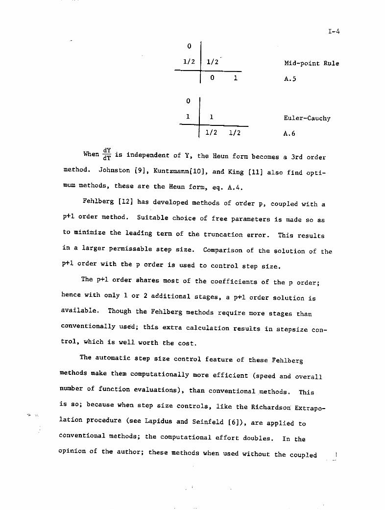
I-4
0
1/2 1/2 Mid-point Rule
0 1 A.5
0
1 1 Euler-Cauchy
1/2 1/2 A.6
dYWhen is independent of Y, the Heun form becomes a 3rd order
method. Johnston [9], Kuntzmann[10], and King [11] also find opti-
mum methods, these are the Heun form, eq. A.4.
Fehlberg [12] has developed methods of order p, coupled with a
p+l order method. Suitable choice of free parameters is made so as
to minimize the leading term of the truncation error. This results
in a larger permissable step size. Comparison of the solution of the
p+l order with the p order is used to control step size.
The p+l order shares most of the coefficients of the p order;
hence with only 1 or 2 additional stages, a p+l order solution is
available. Though the Fehlberg methods require more stages than
conventionally used; this extra calculation results in stepsize con-
trol, which is well worth the cost.
The automatic step size control feature of these Fehlberg
methods make them computationally more efficient (speed and overall
number of function evaluations), than conventional .methods. This
is so; because when step size controls, like the Richardson Extrapo-
lation procedure (see Lapidus and Seinfeld [61), are applied to
conventional methods; the computational effort doubles. In the
opinion of the author; these methods when used without the coupled

I-5
rl order method, are still useful because the TEB has been carefully
minimized. The p+l order method can also be used by itself.
Henceforth Fehlberg methods will be written as: RKE[(p,V);
(p+l, V+n)] n = 1,2,3---
Fehlberg [12] RKE[(2,2); (3,)]:
0
p=2 1 1 Fehlberg
p=3 1/2 1/4 1/4 A.7
1/2 1/2 - w's for p=2
1/6 1/6 2/3 - w's for p=3
0
1/4 ..1/4 Fehlberg
p=2 27/40 -189/800 729/800 A.8
p=3 1 214/891 1/33 650/891
214/891 1/33 650/891 p=2
533/2106 0 800/1053 -1/78 p=3
A.1-3 RKE(3,3):
The deriving equations for such methods are listed in Fehlberg
[12], and in Ralston [8], as a two parameter family. In Ralston [8]
the TEB was minimized by suitable choices of the two free parameters,
and the 'optimum' method is:
0.
1/2 1/2 Ralston Optimum
3/4 0 3/4 A.9
2/9 1/3 4/9

1-6
Johnston [9], Kuntzm4nn.[10] and King [11] also list such opti-
mum methods.
The two optimum methods of King [11] are, however, of a fourth
dY dYand fifth order when - is independent of Y. Whenq is dependent on
Y his methods have a slightly larger TEB than Ralston's method (the
method which becomes fourth order has a slightly smaller TEB than
the method which becomes fifth order.)
0 King optimum (when
dY1/3 1/3 d- independent of
5/6 -5/12 5/4 Y--fourth order)
1/10 1/2 2/5 A.10
0
.3550510257 .3550510257
.8449489743 -.4021612205 1.247110195
.1111111111 .5124858262 .3764030627
King optimum (when
dYd- independent of
Y--fifth order)
A.11
0
(10-2/11) (10-2v1 3) Kuntzmann6
optimum
(i+6/) -.0581020 .82569396 A.12
.2071768 .3585646 .4342585
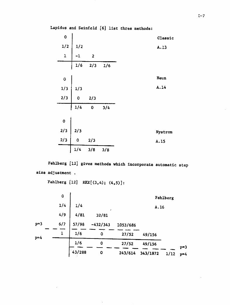
I-7
Lapidus and Seinfeld [6] list three methods:
0 Classic
1/2 1/2 A.13
1 -1 2
1/6 2/3 1/6
0 Heun
1/3 1/3 A.14
2/3 0 2/3
1/4 0 3/4
0
2/3 2/3 Nystrom
2/3 0 2/3 A.15
1/4 3/8 3/8
Fehlberg [12] gives methods which incorporate automatic step
size adjustment .
Fehlberg [12] RKE[(3,4); (4,5)]:
0 Fehlberg
1/4 1/4 A.16
4/9 4/81 32/81
p=3 6/7 57/98 -432/343 1053/686
1 1/6 0 27/52 49/156p=4
1/6 0 27/52 49/156-. --. p=343/288 0 243/614 343/1872 1/12 p=4

I-8
0 Fehlberg
2/7 2/7 A.17
7/14 77/900 343/900
p=3 35/38 805/1444 -77175/54872 97125/54872
p=4 1 79/490 0 2175/3626 2166/9065
79/490 0 2175/3626 2166/9065 p=3
229/1470 0 1125/1813 13718/81585 1/18 p=4
The Fehlberg coupled second order methods, eqa. A.7 and A.8,
could be used as third order methods.
The author developed optimum methods of a special kind, these
methods require only two, instead of three function evaluations per step.
I. Back Step Method:
0
-24/100 -24/100 A.18
76/100 19627/10200 -475/408
409/684 -7/36 36/57
Butcher [18] developed such fifth order processes, using negative
c's. This back step method has a built-in advantage: in every step
except the first; k3 from (T, 1/n) may be used as the k2 for (Tn+I Y n)This results in one less function evaluation per step, hence has V = 2rather than V = 3, a considerable advantage. A disadvantage of back step
methods is that a starting method is required. For a starting method
solve the deriving equations with c3 76 and any choice of c2

1-9
II. Front Step Methods:
0
1 1A.1910 10 A.19
1 133 151 -4 -- 5 -10 170 17
5 1 17-1-- 2-22 6 66
0
1/100 1/100 A.20
101/100 -990103/19700 10000/197
-9994/606 103/6 197/606
These front step methods have a built in advantage: in every
step except the last; k3 from (Tn Y) may be used as the k2 for
(Tn+l' Yn+l) . Like the back step method, this results in a V = 2
rather than V = 3 method. The front step method is self starting
and so has an advantage over the back step method.
Each of the methods eqs. A.18, A.19 and A.20 was optimized using
the procedure found in Ralston [8]. The c2 's and c3's were inter-
changed: a TEB was calculated using a particular c2 and c3 ; then an-
other TEB was calculated using the same c2 as a c3 , and the same c3as a c2 . Eqs. A.18, A.19 and A.20 are the resulting optimum methods.
Method (p, V) Error Bound (TEB)
Ralston A.9 (3,3) .1111 ML3h4
King A.10 (3,3) .1389 ML3h4
King A.11 (3,3) .1391 ML3h4
Classis A.13 (3,3) .5 ML3h4
Heun A.14 (3,3) .6667 ML3h4
Nystrom A.15 (3,3) .25 ML3h4
Back step A.18 (3,2) .3493 ML3h4
Front step A.19 (3,2) .3933 ML3h4
Front step A.19 (3,2) .3649 ML3h 4

I-10
A.1-4 RKE(4,4):
More has been written and analyzed about the RKE(4,4) than any
other Runge-Kutta method. The references listed here try to sample
all the aspects of these methods.
The deriving equations are listed in Butcher [3], Rosen [5],
Ralston [8], and Fehlberg [12].
Ralston [8] gives an optimum method (minimum TEB).
0
.4 .4 Ralston Optimum
.45573725 .29697761 .15875964 A.21
1 .21810040 -3.05096516 3.83286476
.17476028 - .55148066 1.20553560 .17118478
In King [11], two optimum methods are derived, both whose TEB's
are larger than Ralston's optimum, eq. A.21. The first of these be-
dYcomes fifth order, and the second, sixth order when is independentsT
of Y.
0 King
(4- 7)-) 4 - V) A.2210 10
(4 + V6) -(11 + 4 /) (42 + 13V6)10 25 50
1 (1 + 5/) -(3 + 2) (9 - 6)4 2 4
0 (16 - V') (16 + / ) 136 36 9

0 King
(5 - /i) (5 - /) A.2310 10
(5 + /f) -(5 + 3/5) (3 + vr)10 20 4
1 (-1+5V5) -(5 + 3) (5 - /)4 4 2
1 5 5 112 12 12 12
Kuntzmann [10] developed an optimum method close to Ralson's
optimum, eq. A.21.
0 Kuntzmann
2/5 2/5 A.24
3/5 -3/20 3/4
1 19/44 -15/44 40/44
55/360 125/360 125/360 55/360
Hull and Johnston [13] point out that, c2 .35 and c3 .45
(solve deriving equations for remaining coefficients) lead to a
minimum TEB. As previously mentioned in A.1-2, these bounds are
usually larger than the actual error.
Lapidus and Seinfeld [6] list four methods; one of these,
the Gill form, is optimized for round-off errors (has a larger
TEB than Ralston's optimum).

1-12
0 Gill
1/2 1/2 A.25
1/2 (72 - 1) (2 - r2)2 2
1 (+ (/2 )2 2
1/6 ('2 - 2) (v2 + 2) 16 6 6
o Classic
1/2 1/2 A.26
1/2 0 1/2
1 0 0 1
1/6 1/3 1/3 1/6
0 Kutta
1/3 1/3 A.27
2/3 -1/3 1
1 1 -1 1
1/8 3/8 3/8 1/8
Method (p,V) Error Bound (TEB)
Ralston A.21 (4,4) .0546 ML4h5
King A.22 (4,4) .0944 ML 4h5
King A.23 (4,4) .1218 ML4h5
Gill A.25 (4,4) .0882 ML 4h 5
Classic A.26 (4,4) .1014 ML4h5
Kutta A.27 (4,4) .0991 ML4h5
Tests made by the author showed that the Gill and Classic forms
are equal on accuracy while the Ralston form is superior to both these.

Hull [19] gives a good discussion on the problem of optimizing
Runge-Kutta and predictor-corrector type methods.
The ambivalence of the minimum TEB measure can be pointed out;
according to Luther and Sierra [14], using their own minimum TEB
measure, the Kutta form, eq. A.27 is optimum for truncation error.
Blum [15] claims to wipe out the optimum round-off error ad-
vantage of the Gill form, eq. A.25, by modifying the arithmetic
(computer) sequence of the Kutta form, eq. A.27, making it comparable
to the Gill form. Fyfe [16] extends this procedure to any RKE(4,4)
(though these modifications require extra programming effort).
Lawson [17] derives a RKE(4,4) with an extended region of sta-
bility; for integrating ordinary differential equations with large
Lipschitz constants. This is comparable to the other RKE(4,4)'s
on accuracy but can take larger step-sizes. Gates [26] gives a
RKE(4,5).
Fehlberg [12] lists two methods with his usual feature of
automatic step size control (see section A.1-2). Also eqs. A.16
and A.17, Fehlberg third order methods, have fourth order methods
coupled, these can be used separately as fourth orders.
0 Fehlberg
2/9 1/9 A.28
1/3 1/12 1/4
3/4 69/128 -243/128 135/64
p=4 1 -17/12 27/4 -27/5 16/15--------------------
p=5 5/6 65/432 -5/16 13/16 4/27 5/144
1/9 0 9/20 16/45 1/12 p=4
47/450 0 12/25 32/225 1/30 6/25 p=5

I-14
0 Fehlberg
1 1 A.294
3 3 98 32 32
12 1932 7200 729613 2197 2197 2197
439 3680 845p=4 1 -8
216 513 4104
1 8 3544 1859 11p=5 27 2 2565 4104 40
25 1408 2197 1216 2565 4104 5
16 ! 6656 28561 9 2
135 12825 56430 50 55
Sarafyan [28] RKE[(4,4); (5,6)]
0
1 12 2 Sarafyan
1 1 124 A.30
p=4 1 0 -1 2
2 7 10 10 --
3 27 27 0 27
1 28 125 546 54 378p=5 5 625 625 625 625 625
11 0 2 16 3 6 p=4
141- 0 0 35 162 125
336 336 336 p=5
Fehlberg [12] tested the above three methods, eqs. A.28, A.29
and A.30. Eq. A.28 was the best on accuracy, while eq. A.29 was the
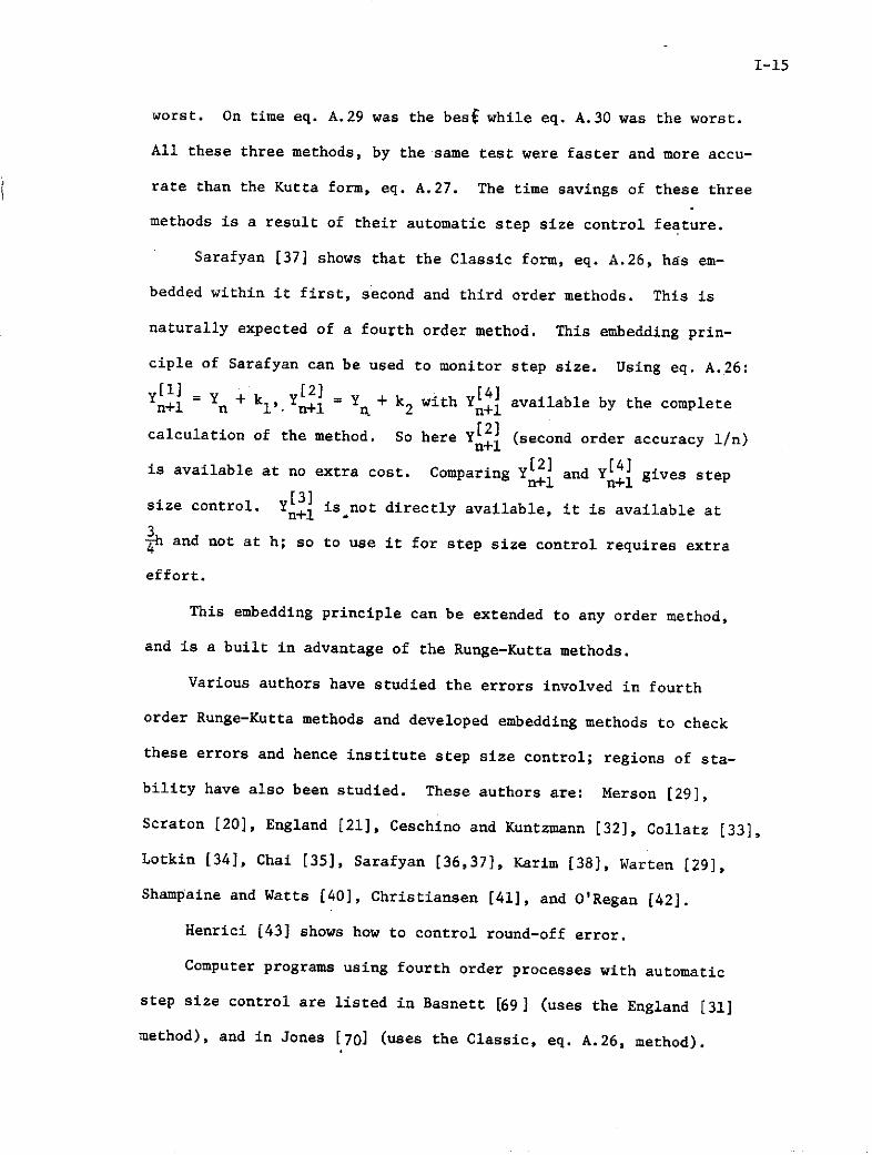
1-15
worst. On time eq. A.29 was the besf while eq. A.30 was the worst.
All these three methods, by the same test were faster and more accu-
rate than the Kutta form, eq. A.27. The time savings of these three
methods is a result of their automatic step size control feature.
Sarafyan [37] shows that the Classic form, eq. A.26, has em-
bedded within it first, second and third order methods. This is
naturally expected of a fourth order method. This embedding prin-
ciple of Sarafyan can be used to monitor step size. Using eq. A.26:
y[l] + [ 2 ] y + wn+l n Y + kl'. Y + k2 with Y +4] available by the completenll n 1 n+l n 2 n+l
calculation of the method. So here Y 2] (second order accuracy 1/n)
is available at no extra cost. Comparing Y 2] and Y [4]ng n+l n+l gives step
size control. Yn[3 is not directly available, it is available atn+l -
% and not at h; so to use it for step size control requires extra
effort.
This embedding principle can be extended to any order method,
and is a built in advantage of the Runge-Kutta methods.
Various authors have studied the errors involved in fourth
order Runge-Kutta methods and developed embedding methods to check
these errors and hence institute step size control; regions of sta-
bility have also been studied. These authors are: Merson [29],
Scraton [20], England [21], Ceschino and Kuntzmann [32], Collatz [33],
Lotkin [34], Chai [35], Sarafyan [36,37], Karim [38], Warten [29],
Shampaine and Watts [40], Christiansen [41], and O'Regan [42].
Henrici [43] shows how to control round-off error.
Computer programs using fourth order processes with automatic
step size control are listed in Basnett [69] (uses the England [31]
method), and in Jones [70] (uses the Classic, eq. A.26, method).
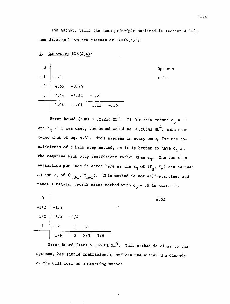
1-16
The author, using the same principle outlined in section A.1-3,
has developed two new classes of RKE(4,4)'s:
I. Back-step RKE(4,4):
0 Optimum
-.1 - .1 A.31
.9 4.65 -3.75
1 7.44 -6.24 - .2
1.06 - .61 1.11 -.56
Error Bound (TEB) < .22254 ML4 . If for this method c 3 = .1
and c2 = .9 was used, the bound would be < .50641 ML , more than
twice that of eq. A.31. This happens in every case, for the co-
efficients of a back step method; so it is better to have c2 as
the negative back step coefficient rather than c3. One function
evaluation per step is saved here as the k3 of (Tn, Yn) can be used
as the k2 of (Tn+1, Yn+). This method is not self-starting, and
needs a regular fourth order method with c3 = .9 to start it.
0 A.32
-1/2 -1/2
1/2 3/4 -1/4
1 -2 1 2
1/6 0 2/3 1/6
Error Bound (TEB) < .26181 ML4. This method is close to the
optimum, has simple coefficients, and can use either the Classic
or the Gill form as a starting method.

1-17II. Front Step Method (4,3):
0
.01 .01
1.01 -50.52 51.53
1 -48.557981 49.548558 .009423
- 8.080858 8.585858 -8.085804 8.580804
Error Bound (TEB) < .23178 ML4. Here again, as in the case ofBack Step methods interchanging values of c2 and c3 results ina bound nearly twice as large, i.e., < .43719 ML4 for c2 = 1.01 andc3 = .01. For this method the k3 of (Tn Y ) can be used as the k2of (Tn+l, Yn+l). One major advantage over the Back Step methods isthat the Front Step methods are self starting. The optimum FrontStep eq. A.33 has a bound not much larger than the optimum Back Stepeq. A.31; so the Front Step methods should have great potential.
As there are only two free parameters in the fourth order case,a back and front step (V = 2) fourth order method is not possible;but as the fifth order case has five free parameters a back andfront step fifth order is possible. The author is working on suchfifth and higher order methods.
On comparing error bounds with the other fourth order methodsit is seen that the bounds of the Front and Back step methods aremuch larger; this is to be expected, and is the price paid forachieving V = 3 in a fourth order method.
A.1-5 RE (5,6):
The RKE(5,6)'s are claimed by many exponents, in the Runge-Kuttafield, to be the best compromise between accuracy and computational ef-ficiency (computer time).

1-18
The deriving equations are presented in Butcher [3], Fehlberg [4],
Luther and Konen [20], Luther [21], Konen and Luther [22]. These also
give general solutions to the deriving equations. The last three
references explore the complete range of solutions possible, in terms
of two and one parameter families. These lead to various Newton-
Cotes, Gauss, Radan and Lobatto family of formulae. Cassity [23],
Cassity [24] and Lawson [25] also state and solve the deriving equa-
tions generally in terms of various free parameters.
Rosen [4] gives deriving equations using the Quadrative approach.
Lapidus and Seinfeld [6] also list a number of RKE (5,6) in-
cluding the Kutta form corrected by Nystom.
0
1/3 1/3 Nystrom
2/5 4/25 6/25 A.34
1 1/4 -12/4 15/4
2/3 6/81 90/81 -50/81 8/81
4/5 6/75 36/75 10/75 8/75 0
23/192 0 125/192 0 -81/192 125/192
I. RKE(5,6) of Newton-Cotes quadrative Familv:
0
1 1 Luther [21]
1 1/2 1/2 A.35
1/4 14/64 5/64 -3/64
1/2 -12/96 -12/96 8/96 64/96
3/4 0 -9/64 5/64 16/64 36/64
7/90 0 7/90 32/90 12/90 32/90
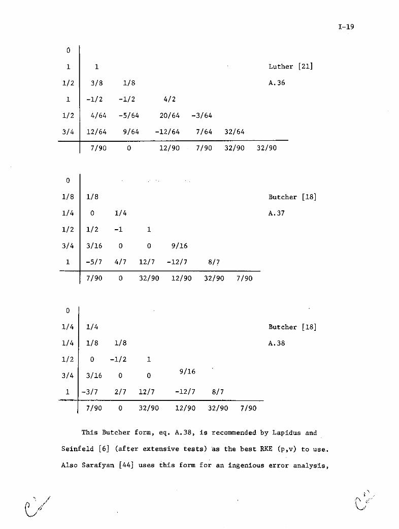
1-19
1 1 Luther [21]
1/2 3/8 1/8 A.36
1 -1/2 -1/2 4/2
1/2 4/64 -5/64 20/64 -3/64
3/4 12/64 9/64 -12/64 7/64 32/64
7/90 0 12/90 7/90 32/90 32/90
0
1/8 1/8 Butcher [18]
1/4 0 1/4 A.37
1/2 1/2 -1 1
3/4 3/16 0 0 9/16
1 -5/7 4/7 12/7 -12/7 8/7
7/90 0 32/90 12/90 32/90 7/90
0
1/4 1/4 Butcher [18]
1/4 1/8 1/8 A.38
1/2 0 -1/2 1
3/4 3/16 0 0 9/16
1 -3/7 2/7 12/7 -12/7 8/7
7/90 0 32/90 12/90 32/90 7/90
This Butcher form, eq. A.38, is recommended by Lapidus and
Seinfeld [6] (after extensive tests) as the best RKE (p,v) to use.
Also Sarafyan [44] uses this form for an ingenious error analysis,
C~ CiN

1-20
hence this form is highly recommended. The author's test show this
method to be the best RKE(5,6) on accuracy.
0
-1/2 -1/2 Butcher [18]
1/4 5/16 -1/16 A.39
1/2 -3/4 1/4 1
3/4 3/16 0 0
1 0 -1/7 12/7 -12/7 8/7
7/90 0 32/90 12/90 32/90 7/90
This Butcher form is of the back step type, discussed in section
A.1-3. This allows in all steps after the first, to use k4 from
(Tn, Yn) for the k2 of (Tn+1,Yn+1 ). Hence, overall, this method
requires V = 5 instead of V = '6. Another such method is (not of the
Newton-Cotes family):
0
-1/5 -1/5 Butcher [18]
2/5 4/5 -2/5 A.40
1/3 7/36 0 5/36
4/5 0 0 4/5 0
1 1/4 0 -35/4 54/7 25/14
5/48 0 0 27/56 125/336 1/24
Here c2 = -1/5 c5 = 4/5 so allows the use of k5 from (TnY ) for
the k2 of (Tn+lYn+). The larger number of zeros present in eq.
A.40 as compared to eq. A.39 should make eq. A.40 more computationally
efficient than eq. A.39.
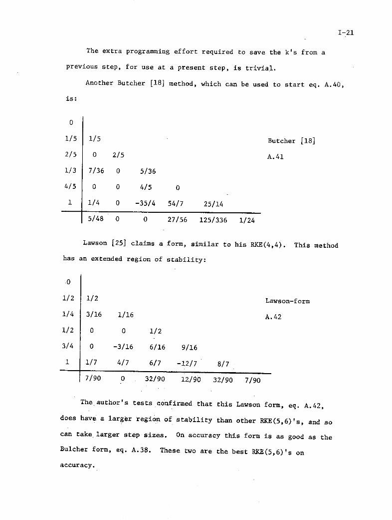
1-21
The extra programming effort required to save the k's from a
previous step, for use at a present step, is trivial.
Another Butcher [18] method, which can be used to start eq. A.40,
is:
0
1/5 1/5 Butcher [18]
2/5 0 2/5 A.41
1/3 7/36 0 5/36
4/5 0 0 4/5 0
1 1/4 0 -35/4 54/7 25/14
5/48 0 0 27/56 125/336 1/24
Lawson [25] claims a form, similar to his RKE(4,4). This method
has an extended region of stability:
0
1/2 1/2 Lawson-form
1/4 3/16 1/16 A.42
1/2 0 0 1/2
3/4 0 -3/16 6/16 9/16
1 1/7 4/7 6/7 -12/7 8/7
7/90 0 32/90 12/90 32/90 7/90
The author's tests confirmed that this Lawson form, eq. A.42,
does have a larger region of stability than other RKE(5,6)'s, and so
can take larger step sizes. On accuracy this form is as good as the
Bulcher form, eq. A.38. These two are the best RKE(5,6)'s on
accuracy.
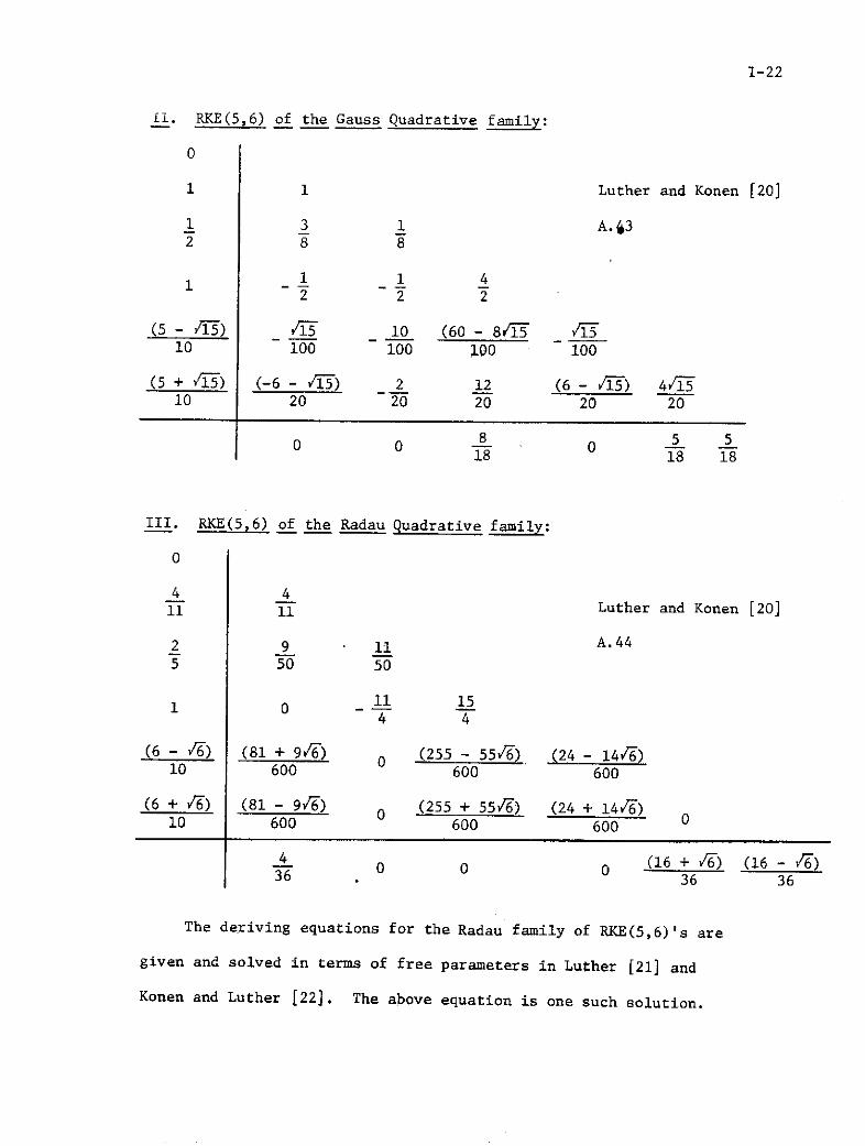
1-22
ii. RKE(5,6) of the Gauss Quadrative family:
0
1 1 Luther and Konen [20]
1 3 1 A.J32 8 8
1 1 41 -- -- 42 2 2
(5 - 1v ) 1- 5 10 (60 - 8/15 4510 100 100 100 100
(5 + /iT) (-6 - ViT) 2 12 (6 - /1-) 4/i-10 20 20 20 20 20
8 5 518 18 18
III. RKE(5 6) of the Radau Quadrative family:
0
4 411 11 Luther and Konen [20]
2 9 11 A.445 50 50
11 151 0 414 4
(6 - Jv) (81 + 9 6) 0 (255 - 55V') (24 - 14/6)10 600 600 600
(6 + /) -) (81 - 9 ) 0 (255 + 55/7) (24 + 14,7)10 600 600 600
4 0 0 0 (16 + /) (16 - )36 36 36
The deriving equations for the Radau family of RKE(5,6)'s are
given and solved in terms of free parameters in Luther [21] and
Konen and Luther [22]. The above equation is one such solution.
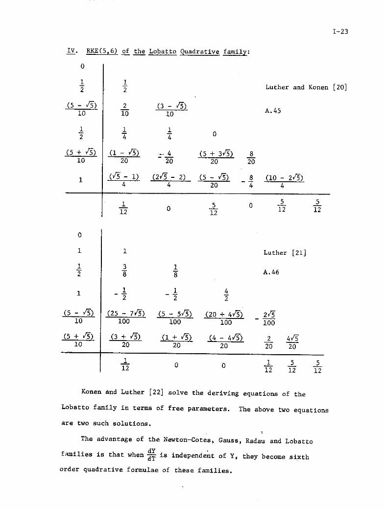
I-23
IV. RKE(5,6) of the Lobatto Quadrative family:
0
1 12 2 Luther and Konen [20]
(5- 1 ) 2 (3 - A.45A.4510 10 10
1 1 12 4 4
(5 + V) (1 - r) .. 4 (5 + 35) 810 20 20 20 20
(Y5 - 1) (2/ - 2) (5- r5) 8 (10- 2r5)4 4 20 4 4
1 5 0 5 5- 0 12 12 12
0
1 1 Luther [21]
1 3 1S- A.462 8 8
1 1 1 42 2 2
(5 - 5) (25 - 7/5) (5 - 5/5) (20 + 4F) 2/10 100 100 100 100
(5 + r) (3 + V5) (1 + r) (4 - 4 Y) 2 4/510 20 20 20 20 20
1 0 0 1 5 512 12 12 12
Konen and Luther [22] solve the deriving equations of the
Lobatto family in terms of free parameters. The above two equations
are two such solutions.
The advantage of the Newton-Cotes, Gauss, Radau and Lobatto
dYfamilies is that when - is independent of Y, they become sixth
order quadrative formulae of these families.

1-24
Luther and Konen [20] point out that, on basis of computational
efficiency, due to the number of zeros present, the Gauss and Radau
forms are better than the Lobatto forms, which in turn is better
than the Newton Cotes form. While 'a round-off error minimization;
following the principle outlined in Gates [26], shows that on
accuracy (based on round-off error), the Lobatto form is better than
the other three.
Shanks [27] developed a class of RKE(5,5)'s rather than RKE(5,6)'s.
This was done by solving the non-linear deriving equation approxi-
mately, not exactly, resulting in one less function evaluation. The
theory for reducing V for RKE's is also given here for p : 7, making
it possible to derive more efficient formulae as compared to the con-
ventional approach. However, it must be pointed out that (in the
opinion of the author) methods derived this way are not exactly p
order, though they are greater than p-1 order. This is because the
truncation error, in such methods has a larger bound. The author's
tests confirmed that Shank's RKE(5,5)'s are faster, though less
accurate than, RKE(5,6)'s.
0
1 11000N 1000N Shanks [27]
3 .(-450N + 3) 450N A.4710 10 10
3 (2250N - 9) 2250N 154 8 8 8
1 (-103500N + 459) 103500N 490 11281 81 81 81
105 500 448 811134 0 1134 1134 11341141134 1134 1134

1-25
Shanks suggests that 1200 Nh 2 > 1 be chosen to give a valid
fifth order method. The author tested values of N from 100,000 to
.0001 and found that N Z 10 gave discrepencies in the coefficients,
while N < 10 does give a valid method. Shanks suggests N = 9.
The author's test with various values of N showed that N = 5 gave
the most accurate method.
The author modified the Shanks form to give a method of four
instead of five stages. This was done by using N = 100, resulting
in 2 1= 1 . As c2 is much smaller than c3, c4 or c5 ; c2 = 0
nc2 100,000 "
was used. This makes k2 = k1 and hence one function evaluation is
saved.
0
0 0 Modified Shanks
3 (-450N + 3) 450N A.48
10 10 10
3 (2250N - 9) 2250N 15
4 8 8 9
(-103500N + 459) 103500N 490 11281 81 81 81
105 500 448 811134 1134 1134 1134
The author's tests showed that this method is faster though
less accurate than the other Shanks forms.
Fehlberg [4] develops methods of order p, coupled with a p+l
order method for automatic step-size control, based on minimizing
the TEB for the p order method as discussed in section A.1-2.

1-26
0
1 11 1 Fehlberg6 6
4 4 16 A.4915 75 75
2 5 8 53 6 3 2
4 8 144 16----- 45 5 25 25
361 18 407 11 55p=5 320 5 128 80 128
11 11 11 110 - 0 -- - 0
640 256 160 256
93 18 803 11 96p=6 640 5 256 160 256
31 5p5 384 661125 9 125-- -- -02816 32 768
7 5 51480 6-6 66
Sarafyan [28] develops similar type methods with step size con-
trol, based on the embedding principle outlined in section A.1-4.
But Sarafyan prefers to control his p order methods by embedded
p-i, i = 1,2,3---, order methods. This requires no extra function
evaluations, so is faster than Fehlberg's methods. But as Fehlberg
uses a p order method controlled by a p+l order method, his error
estimate will be better than Sarafyan; and hence a larger step size
is possible with Fehlberg's methods, at the cost of extra function
evaluations. However the Sarafyan methods can obviously be used in
the same way as the Fehlberg methods, by using the p order method to
control a p-l order solution.
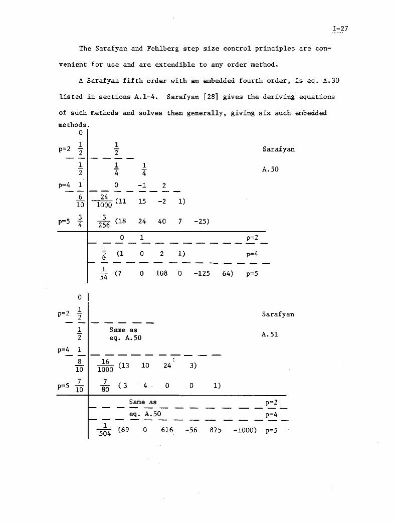
I-27
The Sarafyan and Fehlberg step size control principles are con-
venient for use and are extendible to any order method.
A Sarafyan fifth order with an embedded fourth order, is eq. A.30
listed in sections A.1-4. Sarafyan [28] gives the deriving equations
of such methods and solves them generally, giving six such embedded
methods.0
1 1p=2 12 Sarafyan
1 1 11 A.50
2 4 4
p=4 1 0 -1 2
6 2416 24 (11 15 -2 1)10 1000
3 3p=5 3 3 (18 24 40 7 -25)p=54 256
0 1 p=2
1(1 0 2 1) p=4
1- (7 0 108 0 -125 64) p=5
0
p=2 1 Sarafyan
1 Same as2 eq. A.50 A.51
p=4 1
8 16- 10 (13 10 24 3)10 1000
7 7p=510 - (3 4. 0 0 1)
Same as p=2
eq. A.50 p=4
1---4 (69 0 616 -56 875 -1000) p=5
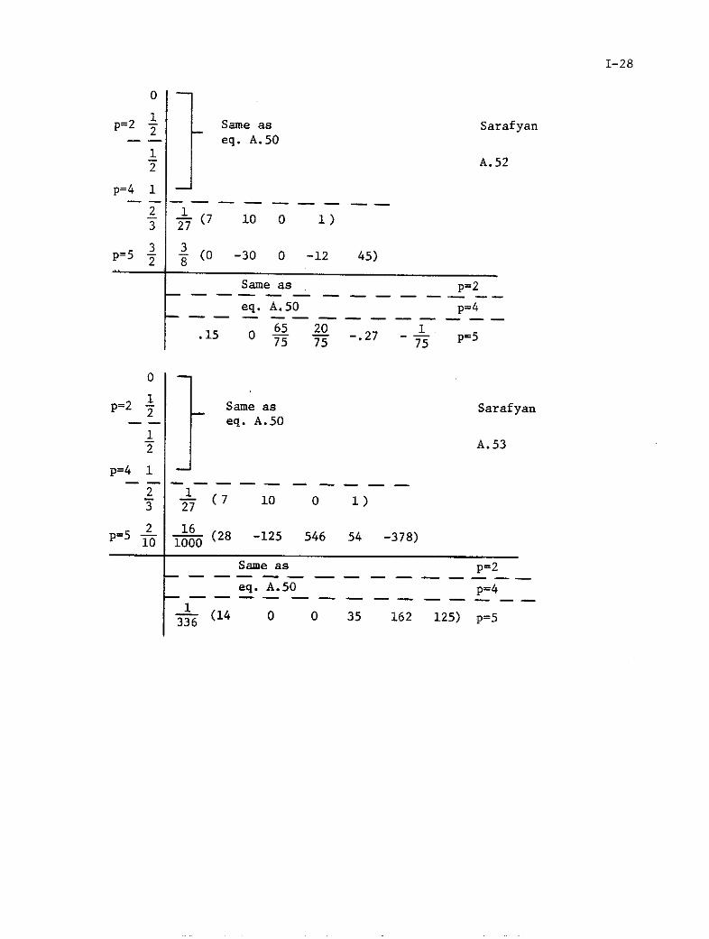
I-28
01
p= 2 -~ Same as Sarafyan- eq. A.50
1A.52
p=4 1
2 1- - (7 10 0 1)
3 3p=5 2 - (0 -30 0 -12 45)
Same as p=2-----------------
eq. A.50 p=4---------------
65 20 1.15 0 - -- -. 27 -- p=575 75 75
0
1p=2 2 Same as Sarafyan
- - eq. A.501
A.53
p=4 1----------------
2 12 1 (7 10 0 1)
2 16p=5 f 1000 (28 -125 546 54 -378)
Same as p=2--- - -'
eq. A.50 p=4-------------------
13-6 (14 0 0 35 162 125) p=5
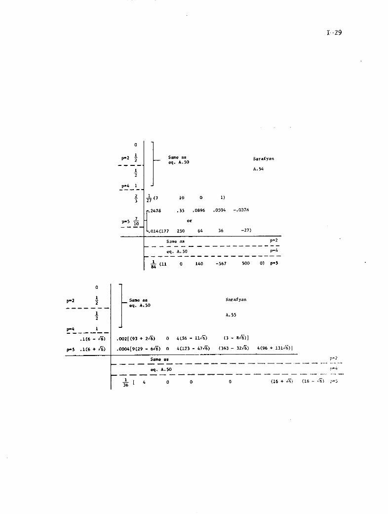
1 -29
0
p-2 I Same aseq. A.50
1 A.542
p-4 1
S--(7 10 0 1)3 27
2478 .35 .0896 .0504 -.0378
p.5 or
.014(177 250 64 36 -27)
Same as p=2
eq. A.50 p=4
(11 0 140 -567 500 0) p-584
p-2 Same as Sarafyan2 eq. A.50
p.4 1
.1(6 - r) .002((93 + 2,6) 0 4(56 - 11") (3 - 84 )]
p-5 .1(6 + r6) .0004[9(29 - 6r) 0 4(123 - 4746) (363 - 3246) 4(96 + 131,/6))
Same as p"2
eq. A.50 6''
6 4 0 0 0 (16 + 1) (16 6-- =536

1-30
All these embedding forms eq. A.50 to eq. A.55 are comparable
to other conventional fifth order methods on accuracy but their
step size control makes them faster.
Sarafyan [44] employs an ingenious step size control with:
0
1/2 1/2 Sarafyan
1/2 1/4 1/4 A.56
1 0 -1 2
3/2 3/8 0 0 9/8
2 -6/7 4/7 24/7 -24/7 16/7
7/45 0 32/45 12/45 32/45 7/45
This form is gotten from the Butcher form, eq. A.38, by multi-
plying all coefficients by a factor of 2. Sarafyan shows that in
going from (Tn, Yn) to (Tn+1 Yn+); using eq. A.38 with h, Yn+l
is available to a fourth order accuracy; at the same time, using
eq. A.50 with 2h, Yn+2 is available to a fifth order accuracy.
Net result - overall V=3 is achieved although the RKE(5,6) of
Butcher is used; and by comparing fourth and fifth order Y n+'s
step size can be controlled.
In the opinion of the author, this Sarafyan method should be
more accurate than eq. A.50 to eq. A.55, because the most accurate
fifth order, eq. A.38, is used here.
A.1-6 RKE(6,7):
The deriving equations are presented in Butcher [3], Fehlberg [4],
and Rosen [5]. The first two also give the general solution of these
equations, in terms of various free parameters.

I-31
In Butcher [3] are listed four RKE(6,7)'s
0
1/3 1/3 Butcher Newton-Cotes
2/3 0 2/3 A.57
1/3 1/12 1/3 -1/12
1/2 -1/16 9/8 -3/16 -3/8
1/2 0 9/8 -3/8 -3/4 1/2
1 9/44 -9/11 63/64 18/11 0 -16/11
11/120 0 27/40 27/40 -4/15 -4/15 11/120
A back step and front step type method (see sections A.1-3 and
A.1-4) is also listed.
0
1 1 C Butcher Newton-Cotes
2/3 4/9 2/9 A.58
1/3 11/36 1/9 -1/12
-1/3 151/36 29/9 -7/4 -6
4/3 -112/9 -116/9 32/3 18 -2
1 -5/4 -29/9 397/276 152/69 -10/69 1/69
23/160 0 29/80 29/80 -1/160 -1/160 23/160
In eq. A. 58 k3 from (Tn, Y n) can be used for the k5 of (Tn+l'
Yn+1); and the k6 of (Tn, Yn) can be used as the k4 of (Tn+1 Yn+l).
So overall V=4 is achieved, hence this method is highly recommended.
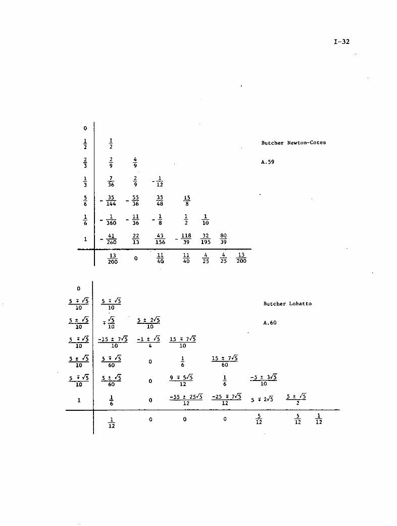
1-32
0
1 1 Butcher Newton-Cotes2 2
2 2 4 9A.59
1 7 2 13 36 9 12
5 35 55 35 156 144 36 48 8
1 1 11 1 1 16 360 36 8 2 10
41 22 43 118 32 80260 - Y5- -T- - - -S 200 13 156 39 195 39
13 11 11 4 4 13200 40 40 25 25 200
0
5 5 5 ; Butcher Lobatto10 10
5 r- A 5 .6010 10 A.60
5 i r -15 ± 7/5 -1 ± 5 15 : 7/10 10 4 10
5 . r 5 :5 0 1 15 * 7F10 60 6 60
5 ; r5 5 ± 0 9 ; 55 1 -5 ± 3/510 60 12 6 10
1 1 0 -55 ±25/'5 -25 . 7,/5 5 2/' 5 f"6 12 12 2
5 5 .1So o o I1012 12 12
12
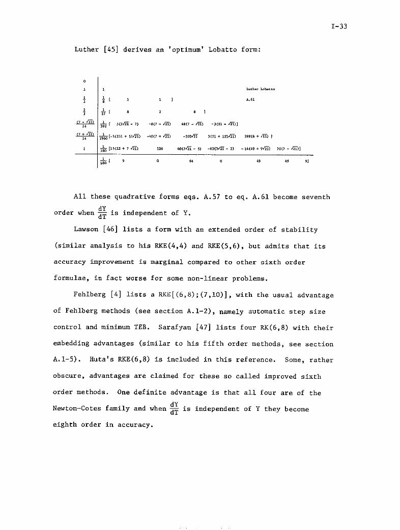
1-33
Luther [45] derives an 'optimum' Lobatto form:
0
1 1 Luther Lobatto
S [ 3 1 j A.61
S1 8 2 8 ]
14 321 [
3(32s - 7) -8(7 - /21) 48(7 - 2") -3(21 - 2')]
Q14 1 [- 5
(231
+ 51Sl) -40(7 + 2/2) -3202i7 3(21 + 121A) 392(6 + 21)
1 [15(22 + 7 2) 120 40(7,2, - 5) -63(3/i - 2) -14(49 + 942/f) 70(7 - /i2)]
[ 9 0 64 0 49 49 9]
All these quadrative forms eqs. A.57 to eq. A.61 become seventh
dYorder whendT is independent of Y.
Lawson [46] lists a form with an extended order of stability
(similar analysis to his RKE(4,4) and RKE(5,6), but admits that its
accuracy improvement is marginal compared to other sixth order
formulae, in fact worse for some non-linear problems.
Fehlberg [4] lists a RKE[(6,8);(7,10)], with the usual advantage
of Fehlberg methods (see section A.1-2), namely automatic step size
control and minimum TEB. Sarafyan [47] lists four RK(6,8) with their
embedding advantages (similar to his fifth order methods, see section
A.1-5). Huta's RKE(6,8) is included in this reference. Some, rather
obscure, advantages are claimed for these so called improved sixth
order methods. One definite advantage is that all four are of the
dYNewton-Cotes family and when dT is independent of Y they become
eighth order in accuracy.

I--34
0
2 233 33 Fehlberg
4 4
33 33 A.62
2 1 0 311 22 22
1 43 0 165 772 64 64 32
2 2383 0 1067 26412 21763 486 54 1701 1701
6 10077 5643 116259 6240 10537 4802 686 16807 16807 2401
1 733 0 141 335763 216 4617 7203p-6 176 8 23296 77 2816 9152
15 --0 35 0 5445 18 1215 1029
352 46592 77 5632 18304 0
1 1833 141 51237 18 729 1029
p-71 -5 0 0 1p7 352 0 8 3584 7 512 1408
771440 270 p-6
- - --- 0 0 1771561 32 243 168076289920 105 2560 74880
11- o 11 11864 0 0U- 11 p-7
270 270 p-7
Y6(T + h) Yn + [41(kl+k 8 ) + 216(k3+k) + 27(k +k6) + 272k56n k 840 k 7 4 k6 2 5]
where
k1 hf(Tn,Yn ) Huta
k2 = hf(T n + h, Yn + ) A.63
k3 " hf(T n + h, Yn + (k2 + 3k3))
k4 hf(T +h, Y + (k1 - 3k2 + 4k3))
k5 - hf(Tn + , Y + (-5k1 + 27k 2 - 24k 3 + 6k4))
6 - hf(T + h, Yn + (221k1 - 981k2 + 867k 3 - 102k4 + k5))
5 1k7 hf(T n +h, Yn + (-183k1 + 678k2 - 472k3 - 66k 4 + 80k 5
+ 3k ))
k = hf(T + h, Yn + 2 (716k - 2079k2 + 1002k 3 + 834k4 - 454k5 - 9k + 72k7).8 n n 2 2 4- - 6 ~ 7

1-35
Y6(T + h) = Y + 41(kl+k8) + 216(k3 +k7) + 27(k 4+k6) + 272k 5]
where
k I = hf(TnYn)
1 1k2 = hf(T n + h, Yn + kl) Sarafyan
k3 = hf(Tn + , Yn 624 (k1 + 3k2)) A.64
k4 = hf(Tn + ~, Yn + (k - 3k 2 + 4k3 ))
k5 = hf(Tn + -4 Yn + (kl + 3k4))
k6 = hf(Tn + h, Yn + (-4kl - 21k2 + 46k3 -29k 4 + 10k5))
5 1k7 = hf(Tn + h, Yn + 2 (-8k1 + 99k2 - 84k3 +44k 4 +9k6))
k8 = hf(T n + h, Yn + (107kl1 - 243k2 + 354k4 - 172k 5 -36k6
+ 72k 7))
kl = hf(Tn Yn)
k2 = hf(Tn + h, Yn + l) Sarafyan
k3 = hf(Tn + h, Y+n + (k1 + 3k2)) A.65
k4 = hf(T +- Y + (kn + Yn + 6 - 3k2 + 4k3))
k5 = hf(T + - Yn + (k1 + 3k4)
k6 = hf(T + h, Y + 2 k - 7k 2 + (16k3 + k
5 f
k7 = hf(Tn +h, Y (-68k1 + 99k2 + 96k3 - 180k 4 + 104k5 + 9k6))
k8 f hf(Tn + h, Yn + (287k1 - 243k2 - 540k3 + 894k4 - 352k5 - 36k6+ 72k7))

1-36
.k1 = hf(Tn Yn)
k2 = hf(Tn + Yn + kl) Sarafyan
k 3 = hf(Tn + h, Yn + (k1 + 3k 2)) A.66
11k4 = hf(T + Y + -6 (k - 3k2
+ 4k3))
k5 = hf(T n + -h, Yn + + 3k4))
2 1k = hf(T +h, Yn + 1 (17kl - 63k + 51k + k))
6 n 3 n 9 1 2 3 5
k = hf(T + ~ Y + 4 (-22k + 33k + 30k - 58k + 34k + 3k6))7 n Yn + 2 1 2 3 4 5 6
k8 = hf(T + h, Y + -2 (281k - 243k - 522k + 876k - 346k8 n n 82 1 2 3 4 5
-36k 6 + 72k7))
Shanks [27] developed an almost (6,6) method on the same
lines as his RKE(5,5), eq. A.47.
1 1300 300
1 29 30Shanks
5 5 5
3 323 330 1055 --- - A.675 5 5 5
14 510104 521640 12705 19255 810 810 810 810
417923 427350 10605 1309 541 - - - - - - - - -77 77 77 77 77
198 1225 1540 810 773696 3696 3696 3696 3696
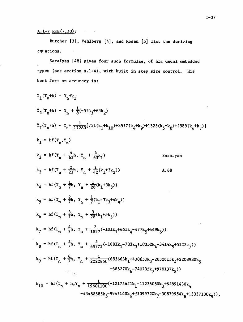
1-37
A.1-7 RKE(7,10):
Butcher [3], Fehlberg [4], and Rosen [5] list the deriving
equations.
Sarafyan [48] gives four such formulae, of his usual embedded
types (see section A.1-4), with built in step size control. His
best form on accuracy is:
Y (T +h) = Y +kl
Y2 (Tn+h) = Yn + L(-55k 1+63k 2)
Y7 (Tn+h) 1 72 8 0 [751(kl+k 1 0)+3577(k4+k9)+1323(k5+k )+2989(k6+k7)]
k I = hf(T ,Y n )
k 2 = hf(T n + 6"' Yn + 3kl ) Sarafyan
2 1k3 = hf(T n + 2l Yn + 2(kl+3k2 ) ) A.68
k4 = hf(Tn + (k1 +3k3))
k5 = hf(Tn + 1h, Yn + f(kl-3k3 +4k 4 ))
k6 = hf(Tn + 1, Yn + (kl+3k 5 ))
4 2k7 = hf(Tn + h, Yn + -2(-10lk 1 +651k 4-477k 5+449k 6))
k8 = hf(Tn + , Yn 5 (-1881k1-783k 3+10352k 4-3414k 5+5122k 7
)
6 1k9 = hf(Tn + h,' Yn + 2 2 2 2 8 5 0 (683663kl+430650k3-2032615k4 +2208930k 5
+385270k6-740735k 7+970137k 8 ) )
k = hf(T + h 1 9 6 0 1100 (- 12175421k -11236050k3+62891430k 4
-43488585k 5-9947140k 6+51099720k 7-30879954k 8+13337100k9 )).
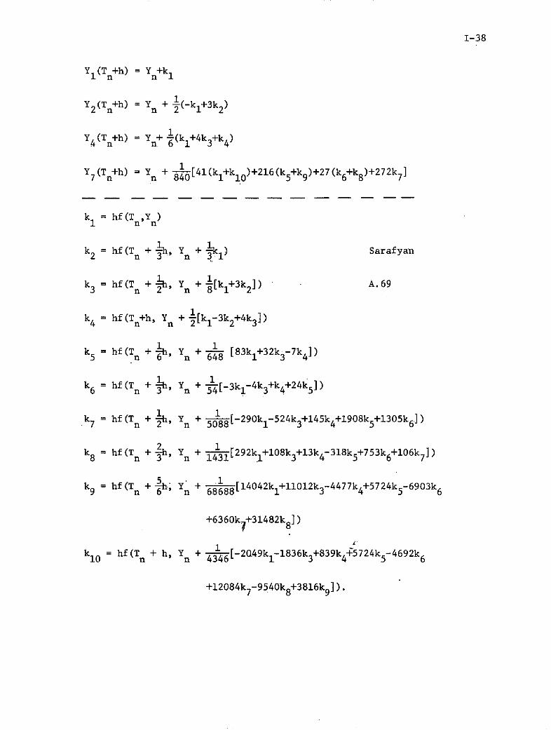
1-38
Y1 (T +h) = Y +k
Y2 (Tn+h) = Yn +-(-kl+3k2)
Y4 (Tn+h) = Y+ -(k+4k 3+k)
Y7(T+h) = Yn+ 0 [41(kl+kl0)+216 (k5+k9)+27(k6+k 8)+272k7]
kI = hf(T ,Y n
k2 = hf(Tn Yn 3 kl) Sarafyan
1
k 3 = hf(T + -=h, Yn + -[kl+3k2] ) A. 69
k = hf(T+h, Yn + -[kl-3k 2 +4k 3])
1 1k 5 = hf(Tn + h, Yn + -48 [83k+32k3-7k 4 ])
k 6 = hf(Tn +h, Yn + 3[-3kl-4k +k 4 +24k 5])
k7= hf(Tn h, 5Y 88[-290kl-524k3+145k +1908k5+1305k67 = 088n 3 4 569 5 +
k8 = hf(Tn +h, Yn 4 3 1 [292kl+108k3+13k 4 318k3+13k-318k5+753k6+106k 7 )
5 1k = hf(T + 68688[14042k +1012k 3-4477k 4+5724k 5-6903k 6
+6360k +31482k8
k10 = hf(T + h, Y + - [-2Q49kl-1836k3+839k 5724k5 -4692k 6
+12084k7-9540k8+3816k9 ]).

1-39
1 (Tn+h) Yn+kl
2Tn+ h )
Yn +
(-25kl+27k2)
7 (Tn+h) - Y + 1 41(k 1+k10 )+216(k+k)+27(k6+k8 )+272k 7
-Y(T + I I
2 (T+ ) Y + (-k+3k 2
y4 (T + ) - + -(k+4k 3 +k 4where
kI . hf(TnYn)
k- hf(T 1
k2 hf(Tn + ih, Yn + jkl) Sarafyan
k3 = hf(T + h Yn + (k+3k2)) A.70
k4 hf(Tn + n + (kl-3k2+4k3))
k5 hf(T + h, Yn+kl+3kL 6 n 414))
and
1 16 -hf(Tn + - Yn + (143k I-420k3+411k -128k )5
k hf( +h, Yn + 1-- (- 2 4 9 4k+6876k 3-5013k 4 +636k+843k6))
2 1
k8 = hf(T n + h, Yn + . (-24
56kl+7548k3-7977k4+3074k-.189k6+106k))
S hf(Tn+ h n + 763( 44946k-118428k
3+89043k 4-7844k5-4431k6-424k 7+3498k8))
k10 = hf(T n + h, Yn + (-67577kl+169308k3-106533k4-3180k +4272k6
+13780k7-954Ok8+3816k9))
or
6 hf( + n + T4(323kl-942k3+915k 4 278k5))
k7 - hf(T n +-h Yn + T (-2070k1+5604k3-3741k4+212k+843k6
k8 = hf(T n +h, Yn + 1 (-244 9
0kl+72132k3-70125k4+23108k 5
-201k 6+848k 7))
kg hf(Tn +h Yn + i (60 3
70k151248k3+96438k +8480k -9747k
+5247k8))
k10 hf(T n + h. Yn + 1(-125084k 1+297912k 3-150897k442824k 5
+14745k6+26288k7-19080k8+7632kg)).

1-40
SYl(T+h) - Yn+k
Y2(Tn+h) - Yn-8k +9k2
LY 7(T+h) - Yn+ [41(kl+k 10 )+216(k5+k 9 )+27(k6+k 8)+272k71
Y(Tn+ h) - Yn+ (-k1
Yh(T+ h) - Y + ) Y (k 1+4k 3+k 4 )
where
k 1 hf(T ,Yn)
k2 " hf(T + 1 Yn + kl )
Sarafyan
k3 = hf(T n + i2' Yn + (kl+3k 2 )) A.71
k hf(T 1 1 +k6 :hf(Tn h. Yn + T2(kl-3k2+k3))
1 , hf(T +h Yn + (kl+4k 2+k 4 ))
and
S6 hf(Tn h Yn + (6kl-12k3+221k 4-206k 5))
k 7 hf(T n + , Yn + - (-115k+448k3-336k 4+215k6))
21k8 hf(Tn + -, Yn + -7(-171k1 +456k 3-8398k 4 +8268k5-49k6+212k ))
kg9 hf(T + + Yn+ f (17367k -52248k 3+36218k4+13144k5-10188k6+5247k8
kl0 hf(T n + h Yn 73 (-11407kl+
35012k 3 ll1631k 4 17490k5+3979k+6572k7-4770k+1908k)
or
6 hf(T n +h, Yn (+
2kl-4k3+109k4104k5))
k * hf(T + h, Yn + (-115k+448k3-548k4+212k5+215k6
k8 - hf(T n +-h, Yn + W7(-171k1+456k3-12426k 4+12296k5-49k6+212k ))
k9 hf(T +hY 136 1 749kk9 hf(Tn +h, Yn + 1-6(5789k 1-17416k 3+19846k 4 5 -3392k5-3396k61749k
k10 hf(T n + h, Y + 1(-11407k1+35012k321277k 7844k +3979k6+6572k7-4770k8+1908k)).10 n n 2173 1 3 - 57

1-41
Fehlberg [4] lists a RKE[(7,11);(8,13)]; with the usual ad-
vantages of this form (discussed in section A.1-2): automatic step
size control and a minimized TEB.
0
2 227 27 Fehlberg
1 1 1 A.729 36 12
1 1 16 24 8
5 5 25 25112 2 16 16
1 1 1 10 02 20 4 5
5 25 125 65 1250 06 108 108 27 54
1 31 61 2 136 300 225 9 900
2 53 704 107 6730 0 6 45 9 90
1 91 23 976 311 19 17 13 108 108 135 54 60 6 12
p=7 2383 0 341 4496 301 2133 45 45 184100 164 1025 82 4100 82 164 41
3 6 3 3 3 60 0 0 0 0 0205 41 205 41 41 41
p=8 1 1777 0 341 4496 289 2193 51 33 124100 164 1025 82 4100 82 164 41
41 41840 840 p=7
34 9 9 9 90 0 0 0105 35 35 280 280
41 41 p=8840 840
Shanks [27] following the approach discussed in section A.1-5,
lists a RKE(7,7) and a RKE(7,9). On a test system, as expected,
the (7,9) was more accurate, while the (7,7) was faster.
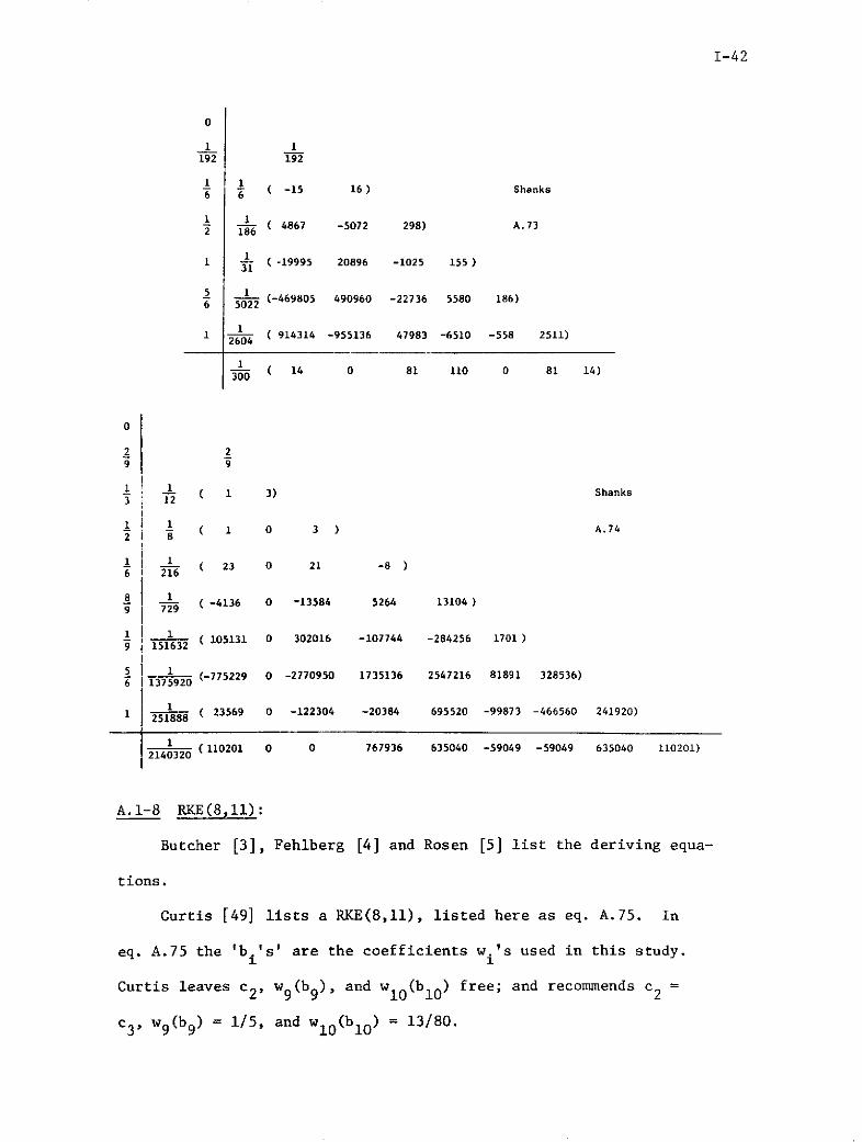
I-42
0
1 1192 192
1 1S( -15 16 ) Shanks
S 1 4867 -5072 298) A.732 186
1 (-19995 20896 -1025 155)
5 1S-22(-469805 490960 -22736 5580 186)
1 ( 914314 -955136 47983 -6510 -558 2511)
1( 14 0 81 110 0 81 14)
0
2 29 9
S ( 1 3) Shanks3 12
1 10 3 A.742 8
1 23 0 21 -8)
8 1 -4136 0 -13584 5264 13104)9 729
( 105131 0 302016 -107744 -284256 1701
S 1 (-775229 0 -2770950 1735136 2547216 81891 328536)
1 ( 23569 0 -122304 -20384 695520 -99873 -466560 241920)251888
1 ( 110201 0 0 767936 635040 -59049 -59049 635040 110201)2140320
A.1-8 RKE(8,11):
Butcher [3], Fehlberg [4] and Rosen [5] list the deriving equa-
tions.
Curtis [49] lists a RKE(8,11), listed here as eq. A.75. In
eq. A.75 the 'b.'s' are the coefficients w.'s used in this study.1 1
Curtis leaves c2, w9 (b9 ), and w1 0 (b1 0) free; and recommends c2
c3, w9 (b9) = 1/5, and w 1 0 (b10 ) = 13/80.

soO lq 0 Ce
9s iss sssio Ai* q /S99I6i4) 1.7*'q- zzzzzzLz~O A-+ 9IZ8ft,3,69- ZZZZZ~LrO += q *9fr LU
o 99czffq t4(IIO-~ '
0o 9 613 OO;V66S Z0 -
o gq 0
sO 0 + 19 0 'eD
0- 4 8S69VI0~fZ900- ='vv
0300O~io, 1 9vt'9t9ziVO + = 1
6lqISi6tlfS- 4-- '"a, s of9 l-SZ0-+ V~v
(6 Z6SZ6SZ6S'o - =1 i~Ot100lqoso4L9SVS-q- lCL0 t9frIWZ+= "T L f sgO(16iof 0o+ = 'U
q;9lt1it6t;i5- - LO 66ZO9 ZZ9O - = "t1 0 = 9!
5LSo6o6tM-i+= '"e 0
SCV 1 161vCI OZS ~ttrs o+ = t'IV
0 =," 169 I(99( WZ90+ = $
ti UL0O 66VtO- V'i" l~~tq po+ = #9
9t9t'9I(qrl*UI+- 12 o 5= 0
o'qI9L6689(lOW0 + = vt 9 t-Z06 t6S90o+~= '
nq/OS 6SzI8000o - = 'VCT l~tu9f96(58SZ+ - P'a
*'9l$99OS6O9ft00 - "vq/t011S6669S000O + D'a' = 18 KO I U'9(6SSV-Z- = ''av
"q9/69 tSo 19 CSV;00 - 2'&v 0 = 9.9v
0'/909 Z 096 (k1400 + O''a' ''V 1,t6zO6 6890o+ = ts'
o 9V3Ma 6( 880LI (SW90t0+ 91
118az090(000 + I*a -V" 0 = I'V
v S 689 zLs80+ = 90 6Z06(t'63900+ = Ps,
,q/ I I z f Z M; o + =- 'IB-6 9sSLOWt'0Sf8vO+= '3
'9i 9IOZO- = A Pe g'3/PC 98VO 069 100+ 1C'
'q,%i 5 (6 1 16(90-0 + = '*0 I" - =
q/ZS 196ZL 9SS17V - 24v - "91 '
1q/069It'g('ZIO0 + p'q'=DI '3

1-44
Fehlberg [4] lists a RKE[(8,15);(9,17)] with his usual advantage
of automatic step-size control and minimum TEB (see section A.1-2).
Fourty digit arithmetic is used for the coefficients of this method.
This is listed here as eq. A.76, where the 's.'s', B..'s', and 'c. s'
are the same as the coefficients, ci, aij and wi respectively, used
in this study. Also in eq. A.76 i and j take values from 0 to 16 while
the formulation used in this study avoids i,j=0. Hence 10 of eq.
A.76 is the usual a21 , c0 is w1 and so on. Naturally a0 (Cl) = 0 in
eq. A.76. A formula for calculating the truncation error is also
listed.

1-45
oz = 0.4436 8940 3764 9818 3109 5994 0428 1370
a2 = 0.6655 3410 5647 4727 4664 3991 0642 2055ot, = 0.9983 0115 8471 2091 1996 5986 5963 3083a4 = 0.3155 0000 0000 0000 0000 0000 0000 0000a-, = 0.5054 4100 9481 6906 8626 5161 2673 7384ft = 0.1714 2857 1428 5714 2857 149.8 714 2857o,7 = 0.8285 7142 8571 4285 7142 8571 4285 7143aa = 0.6654 3966 1210 1156 25:14 9537 6925 5586a9 = 0.2487 8317 9680 626. 2069 7222 7456 0771cao = 0.1090 0000 0000 0000 0000 0000 0000 0000all = 0.8910 0000 0000 0000 0000 0000 0000 0000a12 = 0.3995 0000 0000 0000 0000 0000 0000 0000a13 = 0.6005 0000 0000 0000 0000 0000 0000 0000
C14 = 1
cas = 0
al6 = 1
Bo1 = 0.4436 8940 3764 9818 3109 5994 0428 1370 Fehlbergao = 0.1663 8352 6411 8681 8666 0997 7660 5514B2 = 0.4991 5057 9235 6015 5998 2993 2981 6541 A.76BaD = 0.2495 7528 9617 8022 7999 1496 6490 827103a = 0.7487 2586 8853 4068 3997 4489 9472 491204o = 0.2066 1891 1634 0060 2426 5567 1039 3185B4 = 0.1770 7880 3779 8634 7040 3809 9728 83193o =-0.6819 7715 4138 6949 4669 3770 7681 5048 . 10-1
Bs9 = 0.1092 7823 1526 6640 8227 9038 9092 6157O5s = 0.4021 5962 6423 6799 5421 9905 6369 0087 . 10-2
Os4 = 0.3921 4118 1690 7898 0444 3923 3017 4325060 = 0.9889 9281 4091 6466 5304 8447 6543 4355 • 10-1
063 = 0.3513 8370 2279 6396 6951 2044 8735 6703 . 10-a
Es0 = 0.1247 6099 9831 6001 6621 5206 2587 2489B6s =-0.5574 5546 8349 8979 9643 7429 0146 6348 * 10-
8,~ =-0.3680 6865 2862 4220 3724 1531 0108 06910,4 =-0.2227 3897 4694.7600 7645 0240 2094 4166 . 10+1On = 0.1374 2908 2567 0291 0729 565G 9124 5744 • 10+106 = 0.2049 7390 0271 1160 3002 1593 5409 2206 • 10+13ao = 0.4546 7962 6413 4715 0077 3519 5060 3349 * 10-'

1-46
0146 =-0.6557 0189 4497 4164 5138 0068 7998 52510847 =-0.3908 6144 8804 3986 3435 0255 2024 131008e = 0.2679 4646 7128 5002 2936 5844 2327 1209814 =-0.1038 3022 9913 8249 0865 7698 5850 7427 - 10+10
1410 = 0.1667 2327 3242 5867 1664 7273 4616 8501 * 10+181411 = 0.4955 1925 8553 1597 7067 7329 6707 144181412 = 0.1139 4001 1323 9706 3228 5867 3814 1784 - 10+181413 = 0.5133 6696 4246 5861 3688 1990 9719 1534 * 10-'O1~s = 0.1046 4847 3406 1481 0391 8730 0240 6755 * 10"
81i =-0.6716 3886 8449 9028 2237 7784 4617 8020 * 10"O1m = 0.8182 8762 1894 2502 1265 3300 6524 8999 * 10-2O1sio =-0.4264 0342 8644 8334 7277 1421 3808 7561 * 10-2Oisu = 0.2800 9029 4741 6893 6545 9763 3115 3703 * 10"
1512 =-0.8783 5333 8762 3867 6639 0578 1314 5633 * 10 "
1513 = 0.1025 4505 1108 2555 8084 2177 6966 4009 * 10-1Oiso =-0.1353 6550 7861 7406 7080 4421 6888 9966 - 10+10Bs =-0.1839 6103 1448 4827 0375 0441 9898 82310Bs =-0.6557 0189 4497 4164 5138 0068 7998 5251 Fehlberglmn =-0.3908 6144 8S04 3986 3435 0255 2024 1310B u = 0.2746 6285 5812 9992 5758 9622 0773 2989 A.76 contd.B0w =-0.1046 4851 7535 7191 5887 0351 8857 2676 - 10+1B161o = 0.1671 4967 6671 2315 5012 0044 8830 6588 * 10+18161 = 0.4952 3916 8258 4180 8131 1869 9074 028701612 = 0.1148 1836 4662 7330 1905 2257 9595 4930 - 10+1
01613 = 0.4108 2191 3138 3305 5603 9813 2752 7525 * 10-'B'ss1 = 1
co = 0.3225 6083 5002 1624 9913 6129 0096 0247 * 10-1ca = 0.2598 3725 2837 1540 3018 8870 2317 1963c = 0.9284 7805 9965 7702 7788 0637 1430 2190 - 10-clo = 0.1645 2339 5147 6434 2891 6477 3184 2800cl = 0.1766 5951 6378 6007 4367 0842 9839 7547cvz = 0.2392 0102 3203 5275 9374 1089 3332 0941cis = 0.3948 4274 6042 0285 3746 7521 1882 9325 o 10 2
1,4 = 0.3072 6495 4758 6064 0406 3683 0552 2124 . 10-"
TE = c4 (fo + fr -fm - f ) h
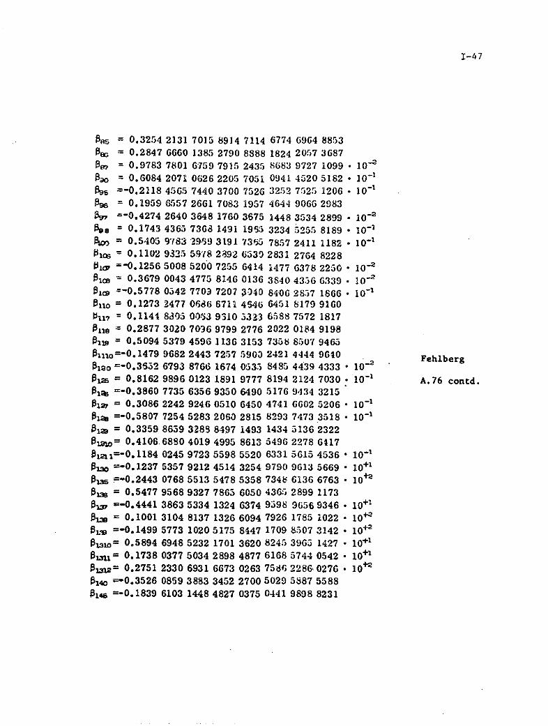
1-47
Bas = 0.3254 2131 7015 8914 7114 6774 6964 8853Oeo = 0.2847 6660 1385 2790 8888 1824 2057 3687BI = 0.9783 7801 6759 7915 2435 8683 9727 1099 * 10 -
8Oo = 0.6084 2071 0626 2205 7051 0941 4520 5182 * 10 - '09s =-0.2118 4565 7440 3700 7526 3252 7525 1206 * 10 - 1
0% = 0.1959 6557 2661 7083 1957 4644 9066 2983s, =-0.4274 2640 3648 1760 3675 1448 3534 2899 * 10-2
O8e = 0.1743 4365 7368 1491 1955 3234 5255 8189 * 10- 'Amo = 0.5405 9783 2959 3191 7355 7857 2411 1182 * 10 - 1
Blos = 0.1102 9325 5978 2892 6539 2831 2764 8228Br1 =-0.1256 5008 5200 7255 6414 1477 6378 2250 * 10 - 2
lc0a = 0.3679 0043 4775 8146 0136 3840 4336 6339 * 10- 2
OIa =-0.5778 0542 7703 7207 3040 8406 2837 1866 * 10-'llo = 0.1273 2477 0686 6711 4646 6451 8179 9160
117 = 0.1144 8d5 00j3 9310 532.3 6588 7572 18178Ole = 0.2877 3020 7036 9799 2776 2022 0184 9198OBiw = 0.5094 5379 4596 1136 3153 7358 8507 9465Ol1o=-0. 1479 9682 2443 7257 5903 2421 4444 9640 FehlbergBlo =-0.3652 6793 8766 1674 0535 8485 4439 4333 * 10-
Olm = 0.8162 9896 0123 1891 9777 8194 2124 7030 . 10 - A.76 contd.B01 =-0.3860 7735 6356 9350 6490 5176 9,434 3215O1a = 0.3086 2242 9246 0510 6450 4741 6602 5206 * 10- '012 =-0.5807 7254 5283 2063 2815 8293 7473 3518 . 10-1
012 = 0.3359 8659 3285 8497 1493 1434 5136 232201aw = 0.4106 6880 4019 4995 8613 5496 2278 6417
x12=-0.1184 0245 9723 5598 5520 6331 5615 4536 . 10-1Sm =-0.1237 5357 9212 4514 3254 9790 9613 5669 . 10+1Om =-0.2443 0768 5513 5478 5358 7348 6136 6763 . 10+23 = 0.5477 9568 9327 7865 6050 4365 2899 1173
Ogw =-0.4441 3863 5334 1324 6374 9398 9656 9346 * 10 + 1
Oun = 0.1001 3104 8137 1326 6094 7926 1785 1022 * 10+-OL' =-0.1499 5773 1020 5175 8447 1709 8507 3142 - 10 +"t31= 0.5894 6948 5232 1701 3620 8245 3965 1427 . 10 + 1
On, = 0.1738 0377 5034 2898 4877 6168 5744 0542 * 10 + ',sAs.= 0.2751 2330 6931 6673 0263 7586 2286, 0276 * 10+2
04o =-0.3526 0859 3883 3452 2700 5029 5887 5588x4s =-0. 1839 6103 1448 4827 0375 0441 9898 8231

1-48
Shanks [27] has listed two 'almost' eighth order formulae (see
section A.1-5), one a RKE(8,10), and the other a RKE(8,12). As
expected the (8,10) is faster, while the (8,12) is more accurate (not
much more accurate, as his own tests prove).
0
4 4
2 12q (1 3) Shanks9 18
1 1 ( 1 0 3) A.77
1 1- g (1 0 0 3)
-~ (13 0 -27 42 8 )
1 14--2 (389 0 -54 966 -824 243 )
1 (-231 0 81 -1164 656 -122 800
5 1S (-127 0 18 -678 456 -9 576 4)
6
1 (1481 0 -81 7104 -3376 72 -5040 -60 720)
j-g ( 41 0 0 27 272 27 216 0 216 41)
0
119 9
1 1( 1 3) Shanks
6 - ( 1 0 3) A.78
-( 29 0 33 -12)
1 (
33 0 0 4 125 )
1 -21 0 0 76 125 -162 )
2 T2
( -30 0 0 -32 125 0 99 )
(1175 0 0 -3456 -6250 8424 242 -27)3 324
5 1( 293 0 0 -852 -1375 1836 -118 162 324)6 324
S 1-- (1303 0 0 -4260 -6875 9990 1030 0 0 162)6 1620
1 4- (-8595 0 0 30720 48750 -66096 378 -729 -1944 -1296 3240)
( 41 0 0 0 0 216 272 27 27 36 180 41)840

1-49
Increasing use of higher precision arithmetic is required, to
realize the advantages of this order over the seventh order (slim
advantage in accuracy)--paying the price of increased computational
time.
A.1-9 RKE's of Ninth and Higher Order
The deriving equations for ninth and higher orders are listed,
but not solved in Rosen [5].
Shanks is supposed to have developed (not yet published) ninth
and tenth order RKE's.
There is no real reason for pushing on for orders beyond the
eighth (except for special problems). According to Fehlberg [4]
accuracy hardly improves after the seventh order methods.
Sarafyan is working on a computer formulation and solution,
of the deriving equations leading to high order methods (see
Sarafyan and Brown [7]); however the results are yet to be published.
A.2 Semi-Implicit Runge-Kutta Methods - RKSI(p,V):
It is easier to use the autonomous form of an ordinary differential
equation system when dealing with these types of methods.
dY- = F(T,Y) A.79
The explicit dependence of T in F(T,Y) can be removed by making
T the (n+l)th component of the n component vector Y. This makes the
system n+l dimensional rather than n dimensional.
let Y+1 = Tn+l

1-50
dYdYn+ldT
dY. = F(Y) A.80dT
where:
Y F1 (Y 'Y"'Y nYn+Y )
dY- = Y and F(Y) = Fi(Y 1"Yi. " Y Y+
Y .
Y Fn(YI **Y.*YY )
n+ 1
The initial conditions would also be accordingly altered,
i.e., Yn+1 (T0 ) = T0 . There is no need however to solve the n+l
component equation of eq. A.80 as its solution is always Yn+ = T.
When a Runge-Kutta method is used on this autonomous form;
the increments coefficients of the abcissa, i.e., the c's, become
a's, i.e., the increment coefficients of the vector component Yn+l"
In Chapter 2, section 2.2 the method of solving for each k.1
of the semi-implicit form was discussed; this involved a Jacobian
inversion. Restating eq. 2.33 in matrix form to apply to a system
of equations, with the a.. 's involved in the Jacobian written as13
a..'a.
i-i i-ik. = [I- haii F (Yn + aj k.] -1 * hF(Y--n + a..j k.)
j=l j=l
A.81i = 1,2,---V
The RKSI type method used to solve eq. A.80 is:

1-51
VY +l= Y + wk
i=1 A.82
k = hF(Y + a kjj=1
To solve for each k. the formulation of eq. A.81 is used.-1
The coefficient matrix is of the form:
all
a2 1 a2 2 a2 1
* *
a a ****a, a a ****a.il i2 ii il 2 ii-
* *
avl a *******...........* avv av a .... avv-v v2 vv vl v2"" vy-1
w w2 ..... w v*** w
Allen [50], Rosenbrock [51] and Haines [52] list the deriving
equations. Allen [50] gives a thorough discussion of the deriving
equations and the stability advantages of RKSI's over RKE's; and also
gives coefficients of the truncation errors. In general RKSI's re-
quire less stages, V per step as compared to RKE's, to achieve a
p order method. The price paid by RKSI's, for achieving extended
stability as compared to RKE;s, is the additional computational ef-
fort required to compute Jacobians and their inverses; but this price
is not As steep as the one paid by RKI's, where iteration for k.'s1
is required.
Lapadis and Seinfeld [6] recommend the use of RKSI only for
those cases where stability is critical, for example, with still
systems; because in general RKSI's are not significantly more accurate
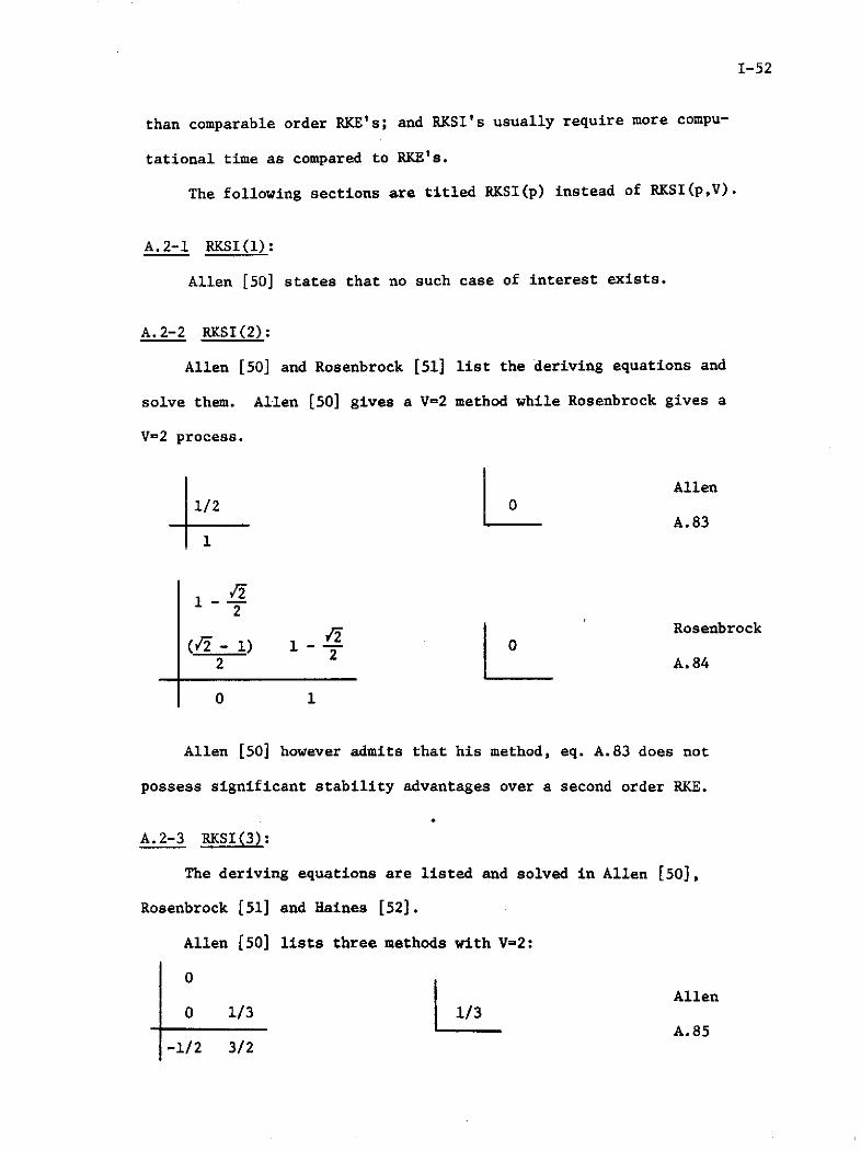
1-52
than comparable order RKE's; and RKSI's usually require more compu-
tational time as compared to RKE's.
The following sections are titled RKSI(p) instead of RKSI(p,V).
A.2-1 RKSI(1):
Allen [50] states that no such case of interest exists.
A.2-2 RKSI(2):
Allen (50] and Rosenbrock [51] list the deriving equations and
solve them. Allen [50] gives a V=2 method while Rosenbrock gives a
V=2 process.
Allen1/2 0
A.831
1
---
0
2,r 1Rosenbrock
(J£ - 1) 1 2 -2 A.84
0 1
Allen [50] however admits that his method, eq. A.83 does not
possess significant stability advantages over a second order RKE.
A.2-3 RKSI(3):
The deriving equations are listed and solved in Allen [50],
Rosenbrock [51] and Haines [52].
Allen [50] lists three methods with V=2:
0Allen
0 1/3 1/3A.85
-1/2 3/2
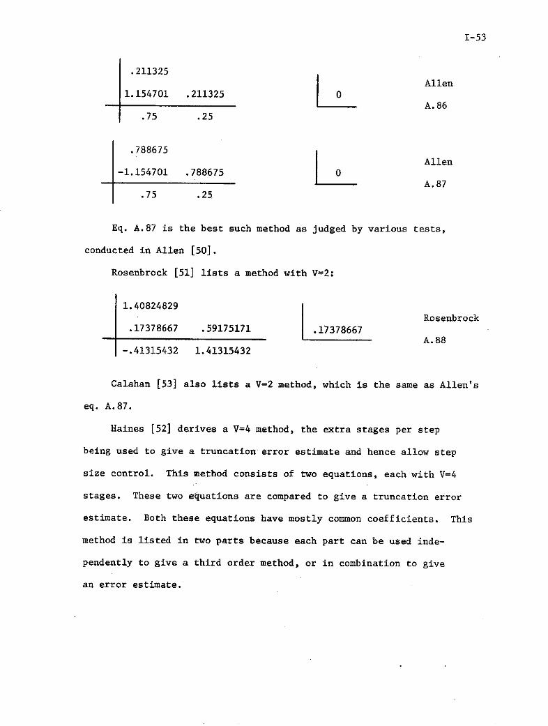
1-53
.211325Allen
1.154701 .211325 0A.86
.75 .25
.788675Allen
-1.154701 .788675 0A.87
.75 .25
Eq. A.87 is the best such method as judged by various tests,
conducted in Allen [50].
Rosenbrock [51] lists a method with V=2:
1.40824829Rosenbrock
.17378667 .59175171 .17378667A.88
-.41315432 1.41315432
Calahan [53] also lists a V=2 method, which is the same as Allen's
eq. A.87.
Haines [52] derives a V=4 method, the extra stages per step
being used to give a truncation error estimate and hence allow step
size control. This method consists of two equations, each with V=4
stages. These two equations are compared to give a truncation error
estimate. Both these equations have mostly common coefficients. This
method is listed in two parts because each part can be used inde-
pendently to give a third order method, or in combination to give
an error estimate.

1-54
1 1 1 Haines
1/2 1/2 1 1/2 1/2 A.89
2/99 95/99 2/99 2/3 0 0 0
19/9 -43/18 28/9 -11/6
1
1 1 1 Haines
1/2 1/2 1 1/2 1/2 A.90
21/44 19/44 1/11 1/2 0' 0 0
10/3 -1 7/3 -11/3
Errorn = (29/9)[(Y n with eq. A.89) - (Yn with eq. A.90)]
Haines [52] also compares his method, which combines eqs. A.89
and A.90 to give step size control, with a RKE(4,4) which uses a simi-
lar step size control. His results point out that his method is
superior on basis of computing time and stability.
A.2-4 RKSI(4):
Allen [50] lists thirth fourth order methods with V=3. Three
such methods are presented here, these three were judged in Allen [50],
and found to be superior to the rest of his methods on some points.
0
- .31447015 .16666667, .4444779 Allen (minimumcomputational
11.8533114 -9.9088335 .16666667 .4444779 0 effort)
3.51324302 -2.57014293 .05689991 A.91
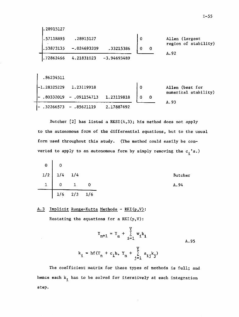
1-55
.28915127
.57118895 .28915127 0 Allen (largestregion of stability)
.53873135 -.024693209 .33215386 0 0A.92
.72862466 4.21831023 -3.94693489
.86234511
-1.28325229 1.23119918 0 Allen (best fornumerical stability)
- .80332019 - .091154713 1.23119818 0 0A.93
- .32266573 - .85621119 2.17887692
Butcher [2] has listed a RKSI(4,3); his method does not apply
to the autonomous form of the differential equations, but to the usual
form used throughout this study. (The method could easily be con-
verted to apply to an autonomous form by simply removing the c.'s.)1
0 0
1/2 1/4 1/4 Butcher
1 0 1 0 A.94
1/6 2/3 1/6
A.3 Implicit Runge-Kutta Methods - RKI(p,V):
Restating the equations for a RKI(p,V):
V
i=l1 A.95
Vk. = hf(T + cih, Y + j aijkj)1 n 1 n j=1
The coefficient matrix for these types of methods is full; and
hence each k. has to be solved for iteratively at each integration1
step.

I-56
The use of these RKI's is recommended for two situatipns: one
where stability is critical and a self-starting process is desired;
two when the differential equation system is such that the cost of
computing f(T,Y) for a given value of T is high compared to the cost
of repeating this computation with Y changed but T unchanged. In
the second situation the iterative nature of an RKI would not be an
objection;especially if the differential equation system is linear,
then the iterations can be replaced by standard linear algebra
techniques.
Advantages: Stability characteristics better than comparable
order RKSI's or RKE's. Always stable for any h.
Higher p for a particular V as compared to RKSI's
and RKE's. The deriving equations are easier to
formulate than those of RKSI's and RKE's.
Disadvantages: For even moderately complex differential equa-
tion systems the iterative solution of ki's re-
quires more computational effort than comparable
order semi-implicit or explicit methods.
The coefficient matrix will be presented in the following form:
.1 .11 .13 .Iv
c. a *" ja..****a..1 . 13 .v
c a ""a.*""av vl vj vv
w .... w. .... w1 3 v
Most currently available implicit processes were derived by
Butcher. The theory behind implicit methods, attainable order, etc.,

1-57
is dealt in Butcher [1] and Verner [54]. Deriving equations and
implicit methods are listed in Butcher [2], Butcher [3] and Butcher
[55]. Lapidus and Seinfeld [6] also list some of these Butcher
methods.
Implicit Runge-Kutta methods are based on quadrative formulae
(The Taylor Series analysis can also be used to derive implicit
methods but the quadrative approach is simpler). Basically Implicit
Runge-Kutta's can be divided into three classes of methods: Gauss-
Legendre quadrative forms, Radau quadrative forms, and Lobatto
quadrative forms.
Quadrative Form Abcissa points (ci's) V pspecified
Gauss-Legendre All c.'s found as roots V 2Vof a ILegendre poly-nomial, no c. specified
i
RadauI c. = 0 specified V (2V-1)
Radaul cV= 1 specified V (2V-1)
Lobatto c1 = 0 and cV = 1 V (2V-2)specified
when cl = 0 all = al2 = al3 = *...... = alV = 0
when cV = 1 alV = a2V = a3V = .= aVV 0
Hence the Lobatto forms have the first row and last column of
the coefficient matrix as zeros. Thus as c1 = 0 and cV = 1 were
specified two ki's, k1 and kV are available explicitly and so can
be solved for by iteration. The RadauI and RadauII forms have only
one k. available explicitly as only one c. is specified. While theSavalable explctly as no c
Gauss-Legendre forms have no k. available explicitly as no c. is1 1

1-58
specified. Because of the number of abcissa points specified, the
Gauss-Legendre forms have the highest p for a given V, while Radau
forms are next and Lobatto forms last.
Butcher [2] also suggests a convergent iterative procedure
applicable for calculating the implicit k.'s of any RKI.
If n is the iteration count for a particular k. the convergent
iterative procedure is:
i-1 V
kn hj(T + c h, Y + a..kn + a..kn l))j=l =i
Butcher proves that this procedure is convergent.
A.3-1 RKI(p,V)'s of the Gauss-Legendre Quadrative forms:
These kinds of RKI's are listed in Butcher [2] from p = 2 to
p = 10 (p = 2V), an error analysis is also included.
1 12 2 RKI(2,1)
A.96
1 - -- RKI(4,2)2 6 - 4 6
1 + 1 I3- 1 A.97
2 6 4 6 4
1 12 2

1-59
S2 035 5i- i- 3 15 36 30 RKI(6,3)
1 % 2 5 7 A.98
I1
2 - , U -U+ - - usu I(8,4)
1 . 0 5 + A.99
+,s 4 +i u us -us us- E1-s
1 , S , A. 100j u+us u s us+
1 1 V
us' (us .. ( _ , + ., us_' - u
. ., + sj--- u + us+ +t- - u- -u
u ua + us u I + usau - s us2s 2s 3
2-225S'f Of 2 s
u su-s+ + O+W o
us us ( ) us' us ( 52- )
405-ea 3

1-60
A.3-2 RKI(pV)'s of the Radau quadrative forms:
These types of RKI's are listed in Butcher [55], from p=l to
p=5 (p = 2V - 1). Butcher [55] also describes an ingenious error
analysis applicable to the Radau and Lobatto (see section A.3-3)
forms of RKI's.
0 0 RKI(1,1)
1 A. 101
0 0 0 RKI(3,2)
2 1 1 A.102333
1 3
O 0 0 0
6) - 9 + \/fi 24 + Wi; 168 - 73 N1' RKI(5,3)10 12 00
o + vi6 9 6- i lIt8 + 73 Vi 24 V- /6 A.103
10 ) 1i(00 120
I ~1 + 16 - vii
1 31 36
1 3 0 RKI(3,2)
1 1 0 A.104
3 14 4
4 - V/i 2- - /i 24 - 1 1i 21 - v - .LYI 0 RKI(5,3)10 120 120
4 + v/i .. + 11 ~1 2-1 + 0/i o A.10510 120 120
1---i . .. - - 012
Il - N/1i Ili + NA~ I:6i 36 T
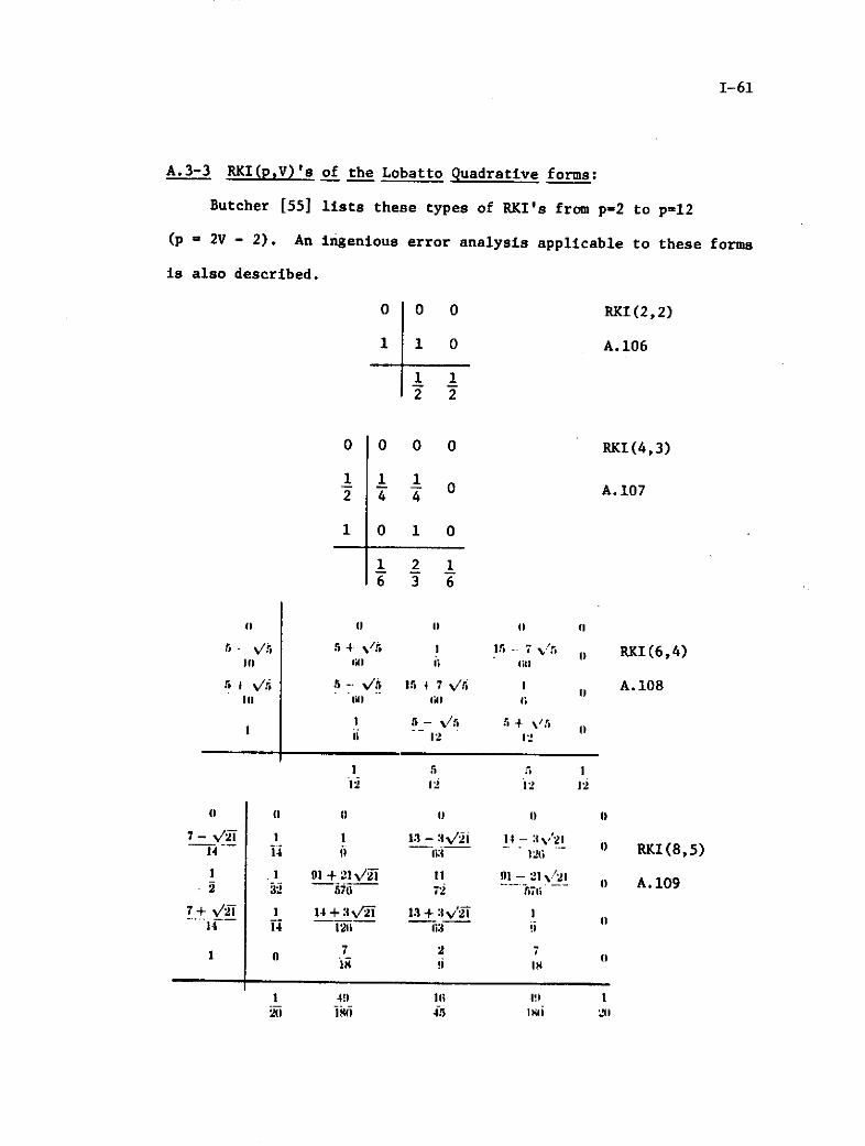
1-61
A.3-3 RKI(p,V)'s of the Lobatto quadrative forms:
Butcher [55] lists these types of RKI's from p-2 to p=12
(p = 2V - 2). An ingenious error analysis applicable to these forms
is also described.
0 0 0 RKI(2,2)
1 1 0 A.106
1 12 2
0 0 0 0 RKI(4,3)
1 1 12 0 A.107
1 0 1 0
1 2 1636
2 I 1 II II (2
,- 5v 4 0, I -15 -t 7 ' RKI(6,4)I4I 0 i2 li1 1
St 8 - 15 7 / I A.108lo lW) lu Ei
+ 1 5- /1j 5- \/5
1 l1
7 - V 1 13 - 3%/ 1. - :V'2114 14 1 -. 126 E- RKI(8,5)
1 .1 1 2/i 11 M - 21 'A1- El - .--- -- A.109
7+ %/Vi 1 14 + :i1 13 + :v"j E...... i--- 1- - F2-6- - i "
1 7 2 7isIi ii IE
-18 45 Imi 21
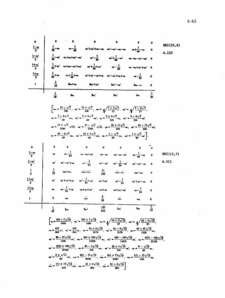
1-62
o 0 0 0 0 00S 1 I(10, 6)
I-1 , 1 11-. rl-+ +4- l'sc' -- 4++ ,-ur +
j + '-' "-u-a'-ug 0A.110
1-+' 1 1 1
+ a+w-,'+a ,+'+ +,, ,a - 4 a-a-a'+' 01 . -I -+ w-+e +.- *w ff' _4+w+ 0
.2 i+,W ,++, +c,'--+< ,'-,O+,+** ,_ 0
11Uwa+"a 201,'+.,, 2 ,a'- ' 2U--- 0
1 2i-n SA S ' 2,' 2"a -
7-5/7 7 , + / 2 + 5VI 2 -5 vr"I M " ) 2) 120
S14 + 714 - + 17/f 22 - 17/i,3714 37) • 340 360
() i0 90
0 0 0 0 0 0 0 0
--- h ,-"+" "-" a-"a-" "-j- 1 RKI(12,7)
2 --4 "- 84
+", W + +, + w , '+ II 0
2 8-84
1 12 8 i
a, o " a, " 0
4 81 25
124 - 7i 124+7v'5 1 +2V1 / _2V1_L" 14 " 1400 33 'Va 33
413 , 413 54 + 5V 5 , 4 - 5B/" OR + 27ViS303' ' ,3 "a 2178 2178 ' '- 320--
9, -27'T 658 + 1. M) , . 58 )- 100 '' 3276 - 1003(1320 4520 14620 27225, 327o+ lO0v13 36 - 4 i ,., +4 ,, 8 - O
"8+ tts , 80I-73vf5 , 86 1+73v5 Ill - 17Vii/ "a, u+_, .. - , a.. ..(10 eco) 0000 (44ows - W - a - - .
O) 30 ' 300
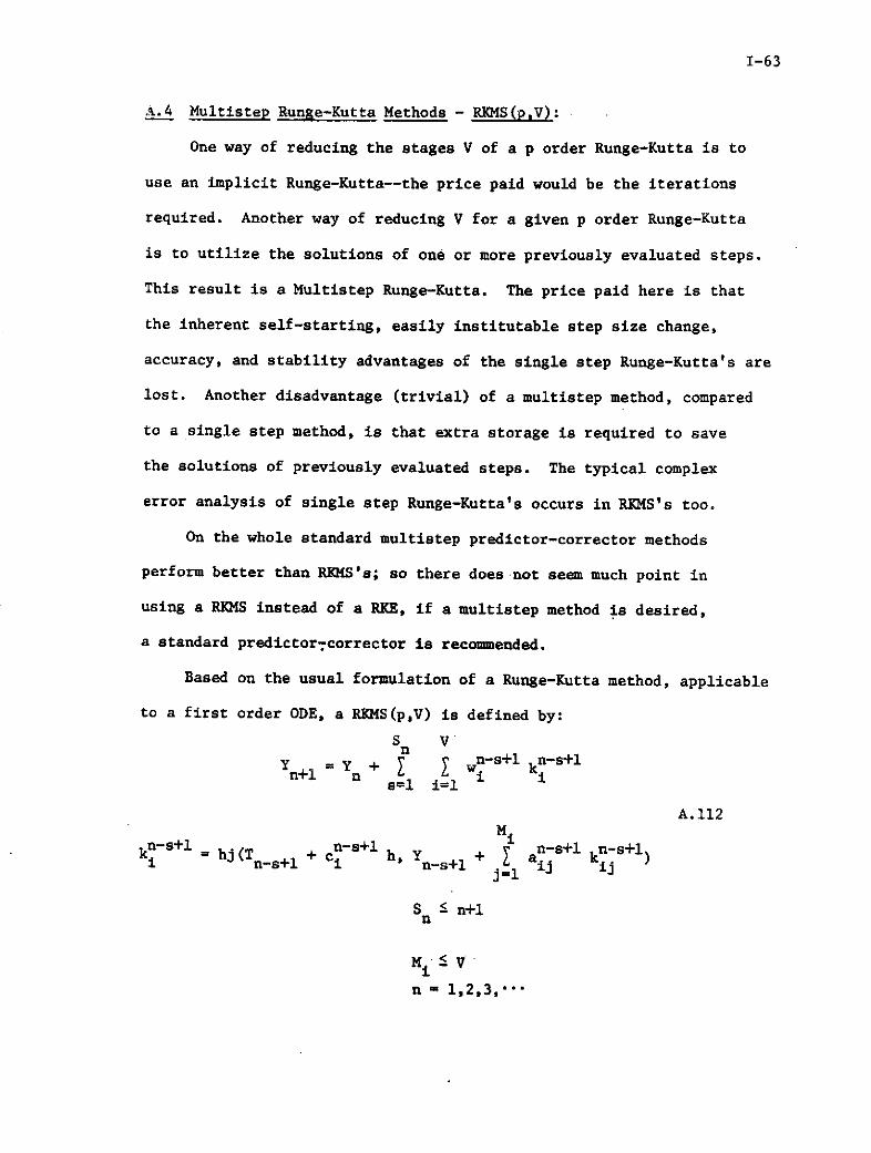
1-63
A.4 Multistep Runge-Kutta Methods - RKMS(p,V):
One way of reducing the stages V of a p order Runge-Kutta is to
use an implicit Runge-Kutta--the price paid would be the iterations
required. Another way of reducing V for a given p order Runge-Kutta
is to utilize the solutions of one or more previously evaluated steps.
This result is a Multistep Runge-Kutta. The price paid here is that
the inherent self-starting, easily institutable step size change,
accuracy, and stability advantages of the single step Runge-Kutta's are
lost. Another disadvantage (trivial) of a multistep method, compared
to a single step method, is that extra storage is required to save
the solutions of previously evaluated steps. The typical complex
error analysis of single step Runge-Kutta's occurs in RKMS's too.
On the whole standard multistep predictor-corrector methods
perform better than RKMS's; so there does not seem much point in
using a RKMS instead of a RKE, if a multistep method is desired,
a standard predictor7 corrector is recommended.
Based on the usual formulation of a Runge-Kutta method, applicable
to a first order ODE, a RKMS(p,V) is defined by:
S Vy y n-s+l n-s+l
n+l n s i1s=l i=l
A.112
kns+l hj(T + cn - s+l h, Y + an-s+ kns+li n-s+l i n-s+l j=l i ij
S S n+ln
M 1S V
n - 1,2,3,-**

1-64
The superscripts in eq. A.112 are used to identify wi , ki, c.
and a at a particular time step. For example, Sn=1 makes eq. A.112
a single step Runge-Kutta; S =2 makes eq. A.112 a two step Runge-Kutta,
and the k.'s of the (n-l)th time step are used together with the k 's
of the nth time step, to arrive at the solution Yn+l" If S =n+l; then
the wolutions of all previously evaluated steps, including the initial
conditions; are used to calculate Yn+1. Henceforth RKMS(p,V,Sn) will
be used to designate these methods. The value of Sn identifies the
number of steps used in the RKMS. Bryne and Lambert 59 show that
there is not much point in going beyond a two step (Sn=2) Runge-Kutta,
because both accuracy and stability of these RKMS's deteriorate as
compared to single step Runge-Kutta's.
The rest of this section will discuss S =2, or two step RKMS's,
eq. A.112 is reformulated in a more convenient form for S =2.n
V VYn+l = Yn + u igi + k.
i=1 i=lMi
gi = hf(T n- + bih, Yn-l + di gi) A.113j=1
Mik.i = hf(Tn + ciJ , Y + aijkj)
j=1
M V
Usually Mi = i-1 is used to give an explicit formulation.
Rosen [62] gives the deriving equations for RIMS(4,3,2) and RKMS
(5,5,2) using the convenient quadrative approach (convenient as com-
pared to the Taylor Series approach). Butcher [56,57] also gives
the deriving equation, but the methods of these papers are really
hybrid methods, not RKMS's, and so come under section A.5.

1-65
Bryne and Lambert [59] present the deriving equations for two
RKM's: a RKMS(3,2,2) and a RKMS(4,3,2). The general solution, error
analysis and proof of convergence is also presented. Bryne [58] gives
the parameters which make the above two methods optimum (minimum TEB
based on the Ralston [8] criteria, see sections A.1-3 and A.1-4).
Lapidus and Seinfeld [6] also list these two methods.
RKMS(3,2,2):
n-1 n
b =0 cl=0
b2=c2 c2=c 2d21=c2 a1=c 2 A.114
(18c2-5)ul=l-w w1 1 1 12c 2
5u2=-w2 w 12c2 12c2
4c2 free, c2 gives an optimum method.
RKMS(4,3,2):
n-1 n
bl=0 c =0
b2=c 2 c2=c 2b3=c 3 c3=c 3
d21=c2 a21=c2'
d31=a31 a3 1=c3-a3 2[2c3 (c3-c2)]
2d =a a = [A.11532 a32 32 [c 2 (4-5c2)]
[4+18c2c3-5(c2+c 3)]
1 1 1 12c 2c3
[4-5c3]
u2 2 [12c 2 (c2-c3)][5c 2-4]
u3=-w1 w3= [12c 3 (c2-c3)]
c2 and c3 are free, c2=.541 and c3=.722779927 give an optimum method.

1-66
Lapidus and Seinfeld 6 also list the above two methods.
These two methods, eq. A.114 and A.115, are not as accurate as
comparable order RKE's (though they are faster).
Chai 60 develops an optimum RKMS(4,3,2) using an ingenious
derivation. Chai notes that if an RKE(4,4) has w2=0 then the k2 can
be reformulated in a multistep form without changing the ci's, aij s,
and wi's of the RKE(4,4). The method is hence defined by the usual
RKE(4,4) formulation but with k2 given differently.
k 2 = hf(Tn,Y n ) + h2c2f' (T,Yn)
A.116h 3 h4 ,,,,
+ e j"'l (T YYn) + f""(T Y) + ...2! 1 n n 3! 2 n9 n
where
c2 # 0
el and e2 are constants.
By using a finite difference approximation for f'(Tn, Yn) in
eq. A.116 Chai arrives at:
k2 = qlk1 + 2Wn-l + q 3 g1 A.117
where:
VY = Y - Yn-l n n-i
V.*. VYn 1 = wig i A.118
i=l
the gi's being the ki's of the previous step.
Thus V=3 is achieved because no function evaluation is necessary
for k2.

1-67
By comparing a Taylor series expansion of eq. A.117, up to second
order terms, with the first two terms of eq. A.116, gives a set of
conditions for the q's.
ql+ 2 + q3 = 1 A.119
q22 + q3 -c2
Thus one q is arbitrary.
An optimum RKMS(4,3,2) is hence formulated by Chai (minimum TEB)
this uses the same ci's, aij's and wi's as the RKE(4,4) from which it
is derived, hence no separate starting method is necessary.
RKMS(4,3,2):
cI =0
26 42 16c2 = c2 q = 1 +-c q =---c 2 q3 c
2 2 1 2 2 5 2 3 5 2
c3 = 1/2
c4 = 1
a21 = c2 A.120
1 1 131 2 8c2 32 '8c2
1 141 2c2 1 a42 - 2 43 2
w1 = 1/6 w2 - 0 w3 w4 = 1/6
c2 = 1/2 or 1/4 is recommended.
Chai's tests show that this RKMS is superior on accuracy and time
to the RKE with which it shares its coefficients. An error expression
for corre-ting the solution, to yield a fifth order accuracy is also
given. De to its simplicity of application and other advantages,
this method is highly recommended.
Gruttke [61] gives the deriving equations for a RKMS(5,4,2).
These equations are solved to yield various methods which are
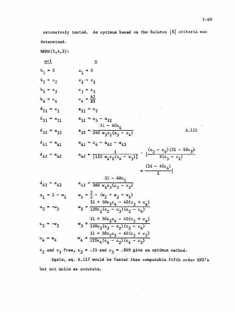
1-68
extensively tested. An optimum based on the Ralston [8] criteria was
determined.
RKMS(5,4,2):
n-1 n
bl = 0 c1 = 0
b2 = c2 c 2 = c2
b3 = c3 c3 = c362
b = 4 4 85
d21 = c2 a21 = c2
d31 = a31 a3 1 = c3 - a3231 - 40c
d = a a 2431- A.12132 = 32 32 240 w3c2 ( 3 - c4)
d41 = a41 a41 = c4 - 42 - a43
1 . (c3 - c4)(31 - 60c3>42 = a42 a4 2 [120 w4 c2 (c4 - c3)] 3(c3 - c2)
(31 - 40c4)+ 2
31 - 60c2
43 = 4 3 43 360 w4 c 3 (c 3 - c2 )
3U1 = - w = (w 2 + w3 + w4 )
31 + 50c3c4 - 40(c 3 + c4)u 2 = 2 w 2 120c2 (c2 - c 3 )(c 2 - c 4 )
31 + 50c 2c4 - 40(c 2 + c 4 )u 3 = -w 3 w 3 +
3 = 3 3 120c3(c 3 - c2 )(c3 - c4 )
31 + 50c 2c3 - 40(c 2 + c 3 )u4 = w4 w4 120c4 (c4 - c 2 )(c 4 - c3)
c 2 and c3 free, c2 = .25 and c3 = .869 give an optimum method.
Again, eq. A.117 would be faster than comparable fifth order RKE's
but not quite as accurate.

I-69
There would be very little advantage in deriving an implicit or
semi-implicit RKMS form (Mi = V or Mi = i in eqs. A.112 or A.113),
because of the additional complexities involved.
A.5 Special Types or Hybrid Runge-Kutta Methods
Two most widely used methods of numerically solving ODE's are
the Runge-Kutta methods and the predictor-corrector methods.
For complex systems of ODE's numerical solutions, using the usual
Runge-Kutta's discussed so far, have one big disadvantage--function
evaluations take up the major portion of the computational time in-
volved. Multi-step predictor-corrector methods require considerably
less function evaluations per step. So obviously reducing the number
of function evaluations (V) of a Runge-Kutta, while retaining some
or all the good points of a Runge-Kutta, would yield good methods.
Some compromise between Runge-Kutta's and predictor-correctors is
indicated.
Single step Runge-Kutta's have certain definite advantages and
disadvantages, and so do the predictor-corrector multi-step method.
Characteristics of Comparable Order Methods
Single Step Runge-Kutta Multi-step predictor-correctors
Advantages: Disadvantages:
1) Self-starting 1) Not self-starting
2) Comparatively good stability 2) Comparatively bad stability
characteristics because single characteristics because multi-
step (so large h possible) step (h comparatively small)
3) Step size and order easily change- 3) Step size and order change not
able at each step. easily instituted at each step.

I-70
Disadvantages: Advantages:
1) Computationally fast as1) May require greater computa-
tional time as comparatively comparatively small number
large number of function evalua- of function evaluations re-
tions required quired (provided not too
many iterations done).
2) No easily computable and ac- 2) Fairly easily computable
curate error estimate available and accurate error estimate
usually available.
3) High order methods involve ex- 3) High order methods easily
tremely complicated deriving deroved/
equations.
Hybrid Runge-Kutta's have been developed to combine the advantages
of the Runge-Kutta and predictor-corrector methods, while trying to
avoid their disadvantages.
Rosser 63 developed a class of ingenious hybrid Runge-Kutta's
with great potential. These methods favorably combine the advantageous
features of Runge-Kutta's and predictor-correctors. They may be de-
scribed as implicit, multi-step, predictor-corrector Runge-Kutta's.
These methods are "Block" methods and proceed by blocks of N
steps. Each block is completely independent of other blocks. The
solutions from previously evaluated steps are only required from,
and used within, a particular block. A large degree of flexibility
is built into these block methods giving them three concrete advantages:
1) Step size is constant within a block but can easily be changed from
block to block
2) Order of accuracy can be varied from block to block by changing

1-71
N, the number of steps constituting a particular block; and by
changing the number of iterations used in each block.
3) Accurate estimates of errors incurred within a block are available
and so give good pointers for the best values of h and N for the
next block.
These "Block" methods result in a considerable savings of function
evaluations and are hence highly recommended. The Rosser "Block"
Runge-Kutta's can be defined using the following formulation:
For a block of N steps:
xl. x x x =x -x =h>0X1 x 0 x2 - X1 n X n-l h
The subscript 0 denotes the starting or initial step, hence
x0o YO are known (from initial values or the results of the
previous block).
YO Starting valuesfor a block A.122
YO' = j (x ,yo)
r = YO + mhf(x0,y0) A.123
yr = f(x, m) A.124m mm
r Z 0 m = 1,2,3, ... N
The superscript r is the iterate count.
r+l h r a'r 'rY1 = Y0 + h[wlY0 + all r + * + almYr +"' + an n
'r+l ' 'r 'r 'rYm Y + h[wY + amlY + " + amm + r + a jmnn ] A.125
r+1 Y + h[wn + an r ... + anm + nn + annYn r
r 0 m = 1,2,3, N
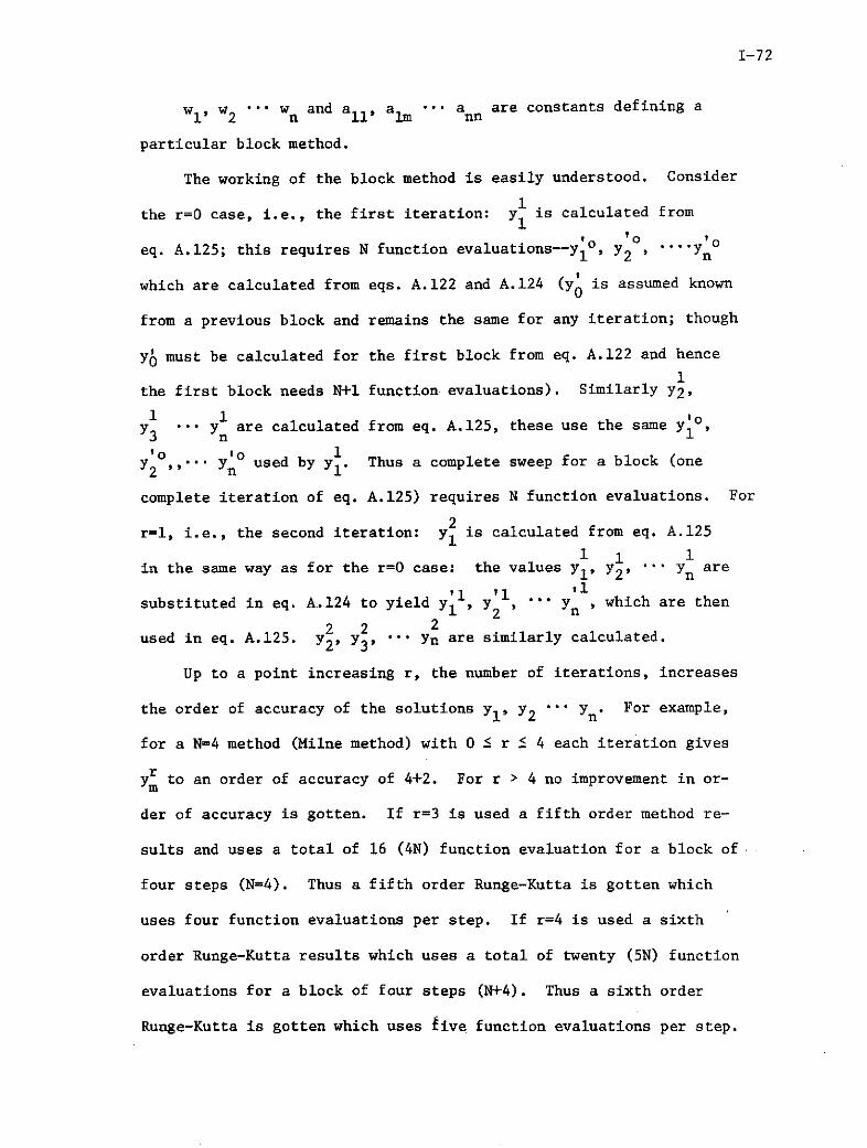
1-72
W, w2 *** Wn and all, a m ", a are constants defining a
particular block method.
The working of the block method is easily understood. Consider
1the r=0 case, i.e., the first iteration: y is calculated from
eq. A.125; this requires N function evaluations--ylo, Y2 , n in
which are calculated from eqs. A.122 and A.124 (y0 is assumed known
from a previous block and remains the same for any iteration; though
yo must be calculated for the first block from eq. A.122 and hence
1the first block needs N+l function evaluations). Similarly y2,
y y. are calculated from eq. A.125, these use the same y '3 n 1
Y2 ' n used by Y 1 . Thus a complete sweep for a block (one
complete iteration of eq. A.125) requires N function evaluations. For
2r=l, i.e., the second iteration: yl is calculated from eq. A.125
1 1 1in the same way as for the r=0 case: the values yl,' 2' '.. yn are
'1 '1 . 1substituted in eq. A.124 to yield yl , y2 . Yn , which are then
2 2 2used in eq. A.125. y2, y3 "'" yn are similarly calculated.
Up to a point increasing r, the number of iterations, increases
the order of accuracy of the solutions yl, y2 ... yn. For example,
for a N=4 method (Milne method) with 0 : r L 4 each iteration gives
yr to an order of accuracy of 4+2. For r > 4 no improvement in or-
der of accuracy is gotten. If r=3 is used a fifth order method re-
sults and uses a total of 16 (4N) function evaluation for a block of
four steps (N=4). Thus a fifth order Runge-Kutta is gotten which
uses four function evaluations per step. If r=4 is used a sixth
order Runge-Kutta results which uses a total of twenty (5N) function
evaluations for a block of four steps (N+4). Thus a sixth order
Runge-Kutta is gotten which uses five function evaluations per step.
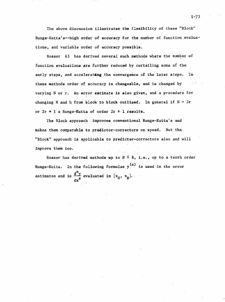
The above discussion illustrates the flexibility of these "Block"
Runge-Kutta's--high order of accuracy for the number of function evalua-
tions, and variable order of accuracy possible.
Rosser 63 has derived several such methods where the number of
function evaluations are further reduced by curtailing some of the
early steps, and accelerating the convergence of the later steps. In
these methods order of accuracy is changeable, and is changed by
varying N or r. An error estimate is also given, and a procedure for
changing N and h from block to block outliaed. In general if N = 2r
or 2r + 1 a Runge-Kutta of order 2r + 1 results.
The Block approach improves conventional Runge-Kutta's and
makes them comparable to predictor-correctors on speed. But the
"Block" approach is applicable to predictor-correctors also and will
improve them too.
Rosser has derived methods up to N I 8, i.e., up to a tenth order
Runge-Kutta. In the following formulae y is used in the errors
estimates and is d- evaluated in [xO, XN].dx

1-74
One-point formulas:
- yo =hyo -+ .+ . A.126
Two-point formulas:
1, - yo = (yo' + yl') - 12 ', ha > - *- -.
U - Yo = 2hyI + h3.
Three-point formulas:
U/ - _ = (o + Sy' - +Y') + A. 128
Y - Yo = 3 (Yo + 4y1 + y') -
3h 3h'y( )
Y3 - YO -T (yo + 3y) + s -
Four-point formulas:
Y - yo= h (9ydo + 19U1' - 5y2' + y3) - 1 A.12924 720
y: - U = h (o' + 4y,' + 1) - '3 90
Y3 - YO = 3 (yo + 3y1 ' + 3y, + yl,) - 3h ,'y
U, - o = (U - Y + 2y3') + 4h'y3 45
S- Y3 = (10yo' - 81y, + 136y3' + 31yG') 3- 160'32 160
Five-point formulas:
Y - Yo = h (251yo' + 646y' - 264y2' + 106ys - 19y') + 3h'16A.130
/2 - Uo = (29yUo + 124y' + 24y2' + 4y3' - y') + " '90 90
U3 -- Y = 3h (9o' + 34y' + 24ys' + 14y3 - yL) + 3h
y, - yo = (7yo' + 32y' + 12y,' + 32y' + 7y') -
Y5 - Uo = 1 (19oy - 10Uy' + 120y2' - 7Oy' + 85y') + 2SS'
U2 - ho -:(, (329yo' + 1.39y!.. - 1216yU' + 45914' - 31ys') -+ I -'"
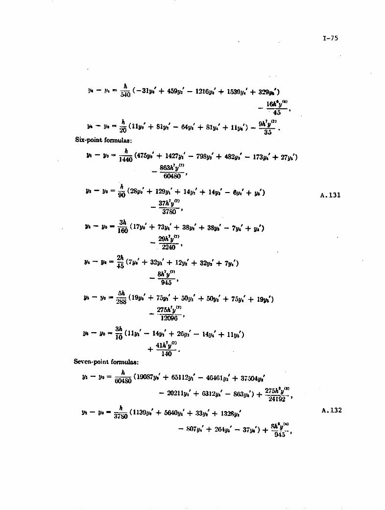
1-75
Y - N = - (-31yo' + 459y:' - 1216y1' + 153j/ + 3291W)
160y( )
.45
Y - o= (11yO + 81y'- y64 + 81y4, + Ilye') - 39 .
Six-point formulas:
- yo = (475yo' + 1427y' - 798y,' + 482ys' - 173y,' + 27y')
863hya)60480'
Y -- (28yo' + 129y,' + 14y2' + 14ys' - 61/. + y/') A. 131
37hy")3780
3hy, - vo - (171o ' + 73y~' + 38y2 + 38y' - 7y4' + y&')
29h'yT)
Y4 - ye =L (7y.' + 32y,' + 12y2' + 32y/' + 7y4')
945
A/s - Io (19yo' + 75y-' + 50y2' + 50y3' + 75y,' + 19y)
275h'yI12096
3kyo - Myo = (llys' - 14y3' + 26y3' - 14y/4' + ly/)
41h'y()
140Seven-point formulas:
s - o = A-- (19087yo' + 65112M ' - 46461ys' + 37504ya'
- 20211y4' + 6312yb' - 83y.') + 275h'y()24192'
h A. 132s - 1o. = S (1139Y ' + 53 6 '10 + 33y;' + 1328y3'
7- -Y,' + 264y' - 37y.') + I)4"043

1--!6
Y3 - u = . ((6vyo' + 3240y' + 1161y' + 2176y3'
- 729y,' + 216y3' .- ,29') + 9hsy896
2hY4 - o = ( 143yo' + 696y,' + 192y2' + 752ya'
+ S7y,' + 24y' - 4y') + Sh' y945
Ys - 2o = 6 ( 743y. + 34SO0y' + 1275y:- + 3200ya'
+ 2325y4' + 112Sy' -- .5 y6') + 2475hy(24192 '
hyo -- = 1:- (41yo' + 216y1' + 27y2' + 272y3'
+ 27y4' + 216y' + 41ye') - 9h'y1400 '
7h7 -YO = g (751yo' - 840y,' + 8547y2 - 1164Sy3
+ 14637y4' - 7224y.' + 4417ys') + 5257Ah'y"17280 '
4hh -- yo = 4 (115yo' + 1312y' - )048y3' + 3132y4'
- 2048y,' + 1312ye' + 113y,) - " 94h y'14175
Eight-point fomnuulas:
A - Uo T (36799yo' + 139849y1' - 121797y2' + z133y A. 133
- 88.547y.' + 41499y,' - 11351ys' + 1375y.') - ;_953hy(362S00 '
Y2 - UO 3 (1107yo' + 5S64yl' - 639y2' + 244Sy'
- 1927y' + 936y -- 261y,' + 32k') - 119h'y16200 '
S- 1U = "- (1325yo' + 6795y' + 1377y2' + 5927 y'
- 3033y4' + 1377ys' - 373y.' + 4504) - 4 6, yO4400 '
2hYU - Yo = 9 (139yo' + 724y,' + 108y2' + S92y'
- 53y,' + 1084' - 32ys' + 4' -' 107hy'1417

1-77
S- = 1412 (8341yo' + 46030yi' + 1510y2' + 63670y3'
- 800y4' + 34186y.' - 9830ys' + 2290y7 - 245ys')
+ 25ho'Yo('3584 '
y -- yo= i (401yo' + 2232y' + 18y?2 + 3224y'
- 360y,' + 2664y' + 15Syl + 72y7 - 9ys')
1400 '
- h = - (21361yo' + 116662y,' + 6958y,' + 155134y3"
+ 7840y' + 105154y' + 7457Sys' + 31882y7' - 1169ya')
8183h'Oy(' 0 )
1036800
Y o = 4 (989yo' + 5888yl' - 92Sy2' + 10496y3'
- 4540y4" + 10496ya' - 92Sy'- + 5888y7' + 989y')
2368777y(5467775
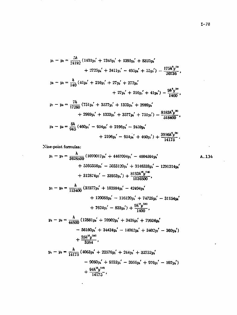
1-78
ys - Yo =4192 (1431yo' + 7345y,' + 1395y,' + S325ya'
+ 2725y4' + 3411y3' - 495y.' + 55y,') - 736 /h
Uy - yo = T (41yo' + 216y,' + 27y,' + 272y3'
+ 27y4' + 216y ' + 41y,/) - 9h'1400
7hY - Yo = Ts (751yo' + 3577y,' + 1323,' + 2989y'
+ 2989y4' + 1323y' + 33577y6' + 751y/) 8183h'y()518400
8hUs - yo = - (460y,' - 954yl + 2196ys' - 2459y4'
+ 2196ya' - 954y.' + 4(60yj) + 3956 y14175
Nine-point formulas:
U' - y0 = (1070017yo' + 4467094yl' - 4604594y,' A. 134
+ 5595358y3' - 5033120y, ' + 314633Sys' - 1291214ye'
+ 312S74y,' - 33953yb') + 8183h'oy n01036S00 '
Y* - Yo = (32377yo' + 182584y,' - 42494y,'
+ 1200Sy; - 116120y,' + 74728yI' - 31154yo'
+ 7624y7' - 833ys') + hly(01400
Y3 - o = (12881yo' + 70902y,' + 3438y2' + 79 934 ys
- 56160y' + 34434y&' - 14062y6' + 3402y/' - 369y3)
25h'Oy 'o)35S4 '
Y4 Y U h (4063yo' + 22576y,' + 244y,' + 32752ya'
- 9080y4' + 9232y' - 3956y6' + 076y/' - 107y&')
94h'oy ('lo14175 '
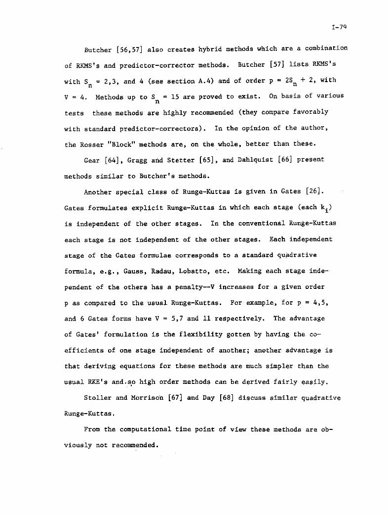
I-7Q
Butcher [56,57] also creates hybrid methods which are a combination
of RKMS's and predictor-corrector methods. Butcher [57] lists RKMS's
with Sn = 2,3, and 4 (see section A.4) and of order p = 2Sn + 2, with
V = 4. Methods up to Sn = 15 are proved to exist. On basis of various
tests these methods are highly recommended (they compare favorably
with standard predictor-correctors). In the opinion of the author,
the Rosser "Block" methods are, on the whole, better than these.
Gear [64], Gragg and Stetter [65], and Dahlquist [66] present
methods similar to Butcher's methods.
Another special class of Runge-Kuttas is given in Gates [26].
Gates formulates explicit Runge-Kuttas in which each stage (each ki)
is independent of the other stages. In the conventional Runge-Kuttas
each stage is not independent of the other stages. Each independent
stage of the Gates formulae corresponds to a standard quadrative
formula, e.g., Gauss, Radau, Lobatto, etc. Making each stage inde-
pendent of the others has a penalty--V increases for a given order
p as compared to the usual Runge-Kuttas. For example, for p = 4,5,
and 6 Gates forms have V = 5,7 and 11 respectively. The advantage
of Gates' formulation is the flexibility gotten by having the co-
efficients of one stage independent of another; another advantage is
that deriving equations for these methods are much simpler than the
usual RKE's and.s.o high order methods can be derived fairly easily.
Stoller and Morrison [67] and Day [68] discuss similar quadrative
Runge-Kuttas.
From the computational time point of view these methods are ob-
viously not recommended.

1-80
4.6 General Comments for Further Development of the Runge-KuttaClass of Methods:
The previous sections have tried to sample various types of Runge-
Kuttas available in current literature.
The field of Runge-Kuttas is wide open and improvements are
possible. Runge-Kuttas in general arrive at an accurate solution at
the end of an integration step, by combining solutions (ki's) at
intermediate steps which are not, in themselves so accurate. So one
way of improving Runge-Kuttas would be to choose the coefficients
of each stage in such a way that the k 's would be accurate estimates
of f(T,Y).
This should be possible without significantly increasing V,
unlike the Gates [26] approach (see section A.5). Then as each k.1
would be an accurate estimate of f(T,Y) a hermitian curve fit would
be possible giving a higher order of accuracy.
The most obvious improvement needed by Runge-Kuttas is to reduce
their stages V per step, this would make them.comparable to predictor-
correctors on computational time. In all other aspects (except error
estimation), i.e., stability and self-starting features Runge-Kuttas
are superior to predictor-correctors. So the second area of improve-
ment lies in reducing V. This is possible to some extent by using
the "Back Step" and "Front Step" methods outlined in section A.1-2,
or by using the Shanks' technique outlined in section A.1-5. Con-
ventional RKE's always have cl=0O and usually have a c.=l, hence the
k. corresponding to the ci=l of the (Tn ,Yn) step could be used for
the ki of the (Tn+,Y n+1) step reducing V by one. This would cost
something--accuracy, because the solution Yn, available at the end of

1-81
(T ,Y ) gives a more accurate estimate for ki than is possible by using
the ki of the previous step. Also if two or more ci's have the same
value, then only one ki corresponding to the first of these cis need
be evaluated. For the rest of these ki's no more function evaluations
are necessary, they can use the same value as the first of these ki's.
Again V is reduced but a loss in accuracy would occur. For example,
1 1a RKE(4,4) which has cl=0, c2= 1, c3= , c4 =1 would become a RKE(4,2)
by using the two techniques outlined above--ki at (Tn+l,Yn+l) would
be the k4 of (Tn,Y n), k3 at (Tn+l1 Yn+1 ) would be k 2 of the same step.
It is not possible to say, off hand, whether the "Back Step" or "Front
Step" technique would be more accurate than this one of interchanging
k.'s. Obviously the interchange techniques could also be used to1
further reduce the V of a "Back Step" or "Front Step" method, with
(probably) a further loss of accuracy, or the Rosser [63] (see section
A.5) "Block" technique could be used to further speed up these methods.
A third area of development (not speed improvement) lies in the
RKSI class of methods. Here a calculation procedure for f or ay
Jacobian is required. As this is available it might as well be used
to improve the order of accuracy, though at the cost of extra compu-
tational effort.
V VYn+l Y n + wiki + C uigi
i=l i=l
i
ki = hf(T n + cih, Y + aijk.) A.135j=1l
Li
gi = h2fy(Tn + dih, Yn + b igj)gj=l
L. V1

1-82
The Rosser [63] (see section A.5) should be applicable to speed up
any type of Runge-Kutta.
Many authors have created hybrid methods which combine Runge-Kutta's
with predictor-correctors, to try and combine the advantages of both
methods (see section A.5). Similarly hybrid methods combining Runge-
Kuttas with extrapolation and other methods should be possible.
The Rosser [63] "Block" technique (see section A.5) could be
adapted to further speed up these hybrid methods. These hybrid
methods may grow to such forms that Runge or Kutta would hardly
recognize their method.
There are other areas in which Runge-Kutta's can be developed
and improved, it is hoped that present and future mathematicians will
do so.
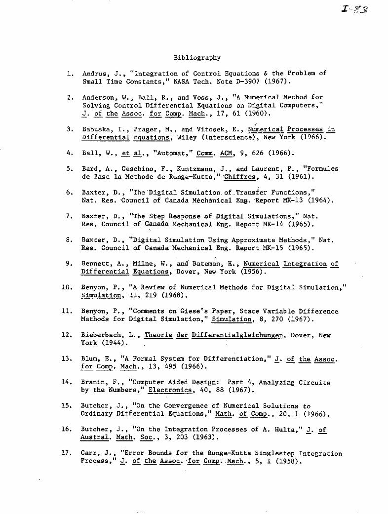
Bibliography
1. Andrus, J., "Integration of Control Equations & the Problem ofSmall Time Constants," NASA Tech. Note D-3907 (1967).
2. Anderson, W., Ball, R., and Voss, J., "A Numerical Method forSolving Control Differential Equations on Digital Computers,"J. of the Assoc. for Comp. Mach., 17, 61 (1960).
3. Babuska, I., Prager, M., and Vitosek, E., Numerical Processes inDifferential Equations, Wiley (Interscience), New York (1966).
4. Ball, W., et al., "Automat," Comm. ACM, 9, 626 (1966).
5. Bard, A., Ceschino, F., Kuntzmann, J., and Laurent, P., "Formulesde Base la Methode de Runge-Kutta," Chiffres, 4, 31 (1961).
6. Baxter, D., "The Digital Simulation of .Transfer Functions,"Nat. Res. Council of Canada Mechanical En. -Report MK-13 (1964).
7. Baxter, D., "The Step Response of Digital Simulations," Nat.Res. Council of Canada Mechanical Eng. Report MK-14 (1965).
8. Baxter, D., "Digital Simulation Using Approximate Methods," Nat.Res. Council of Canada Mechanical Eng. Report MK-15 (1965).
9. Bennett, A., Milne, W., and Bateman, H., Numerical Integration ofDifferential Equations, Dover, New York (1956).
10. Benyon, P., "A Review of Numerical Methods for Digital Simulation,"Simulation, 11, 219 (1968).
11. Benyon, P., "Comments on Giese's Paper, State Variable DifferenceMethods for Digital Simulation," Simulation, 8, 270 (1967).
12. Bieberbach, L., Theorie der Differentialgleichungen, Dover, NewYork (1944).
13. Blum, E., "A Formal System for Differentiation," J. of the Assoc.for Comp. Mach., 13, 495 (1966).
14. Branin, F., "Computer Aided Design: Part 4, Analyzing Circuitsby the Numbers," Electronics, 40, 88 (1967).
15. Butcher, J., "On the Convergence of Numerical Solutions toOrdinary Differential Equations," Math. of Comp., 20, 1 (1966).
16. Butcher, J., "On the Integration Processes of A. Hulta," J. ofAustral. Math. Soc., 3, 203 (1963).
17. Carr, J., "Error Bounds for the Runge-Kutta Singlestep IntegrationProcess," J. of the Assoc. for Comp...Mach., 5, 1 (1958).
1-84
18. Chase, P., "Stability Properties of Predictor-Corrector Methodsfor Ordinary Differential Equations," J. of the Assoc. for Comp.Mach., 9, 457 (1962).
19. Christiansen, J., "Handbook Series Numerical Integration, NumericalSolution of Ordinary Simultaneous Differential Equations of theFirst Order Using a Method for Automatic Step Changes," Num.Math., 14, 317 (1970).
20. Cooper, G., "Interpolation & Quadrature Methods for Ordinary Dif-ferential Equations," Math. of Comp., 22, 69 (1968).
21. Cooper, G., and Gal, E., "Single Step Methods for Linear Dif-ferential Equations," Num. Math., 10, 307 (1967).
22. Davison, E., "A High Order. Crank-Nicholson Technique for SolvingDifferential Equations," Comp. J., 10, 195 (1967).
23. Day, J., "A One-Step Method for the Numerical Integration of theDifferential Equation y" = f (x)y + g (x)," Comp. J., 7, 314(1964).
24. Day, J., "A One-Step Method for the Numerical Solution of SecondOrder Linear Ordinary Differential Equations," Math. of Comp.18, 664 (1964).
25. Ehle, B., "High Order A-Stable Methods for the Numerical Solutionof Systems of Differential Equations," BIT, 8, 276 (1968).
26. Eisenpress, H. and Bomberault, A., "Efficient Symbolic Differen-tiation Using PL/1-FORMAC," IBM New York Scientific Center Report320-29561 (1968).
27. El-Sherif, H., "Implicit Implementation of the Weighted BackwardEuler Formula," IBM J. Res. Develop., 6, 336 (1968).
28. Fehlberg, E., "Eine Methode zur Fehlerverkleinerung beim Runge-Kutta Verfahren," ZAMM, 38, 421 (1958).
29. Fehlberg, E., "Neu Genauere Runge-Kutta Formeln fur Differential-gleichungen n-ter Ordung," ZAMM, 40, 449 (1960).
30. Filippi, S., "Contribution to the Implicit Runge-Kutta Process,"Elektronische Datenverarbeitung, 10, 113 (1968).
31. Filippi, S. and Glasmacher, W., "New Results in Applying theRunge-Kutta Processes with the Aid of Nonnumerical Programs,"Elektronische Datenverarbeitung, 10, 16 (1968).
32. Forrington, C. V. D., "The Numerical Solution of Systems of Dif-ferential Equations Using a Different Step-Length for Each Equa-tion," R.A.E. Tech. Note M.S., 69 (1960).

i-85
33. Fowler, M., "A New Numerical Method for Simulation," Simulation,4, No. 5, 324 (1965).
34. Fox, L., Numerical Solution of Ordinary and Partial DifferentialEquations, Pergamon Press, London (1962).
35. Frey, T., "Solution of Equations by Stepwise Perturbation,"Studia Scientiarum Mathematicarum Nungorica, 3, Nos. 1-3, 93(1968).
36. Froese, C., "An Evaluation of Runge-Kutta Type Methods for HigherOrder Differential Equations," J. of the Assoc. of Comp. Mach.,8, 637 (1961).
37. Gear, C. W., "Rational .Approximations by Implicit Runge-KuttaSchemes," BIT, 10, 20 (1970).
38. Gibbons, A., "A Program for the Automatic Integration of Dif-ferential Equations Using the Method of Taylor-Series," Comp. J.,3, 108 (1960).
39. Gilbert, E. G., "Dynamic-Error Analysis of Digital and CombinedAnalog-Digital Computer Systems," Simulation, 6, No. 4, 24(1966).
40. Gorbunov, A. D. and Shakhov, Y. A., "On the Approximate Solutionof Cauchy's Problem With Ordinary Differential Equations to aGiven Number of Correct Figures," U.S.S.R. Comput. Math. andMath. Phys., 3, 239 (1963).
41. Gorbunov, A. D. and Tikhonov, A. H., "Estimates of Runge-KuttaMethod and the Choice of Optimal Meshes," U.S.S.R Comput Math.and Math. Phys., 4, 427 (1964).
42. Grable, E. M., Ramos, S. and Wollridge, D. E., Handbook of Auto-mation Computation and Control, 1, Wiley, New York (1958).
43. Gray, H. J., "Numerical Methods in Digital Real-Time Simulation,"Quart. Appl. Math., XII, 133 (1954).
44. Gray, H. J., "Digital Computer Solution of Differential Equa-tions," Proceedings of the Western Joint Computer ConferenceAFIPS, 13, 87 (1958).
45. Gray, H. J., "Propagation of Truncation Errors in the NumericalSolution of Ordinary Differential Equations by Repeated Closures,"J. of the Assoc. of Comp. Math., 52, 1, 5 (1955).
46. Grosswald, E., "Transformation Useful in Numerical IntegrationMethods," J. of the Society for Industrial and Appl. Math., 7,76 (1959).

1-86
47. Gurk, H. M., "The Use of Stability Charts in the Synthesis of
Numerical Quadrature Formulae," Quart. Appl. Math. XIII, 73
(1955).
48. Gurk, H. M. and Rubinoff, M., "Numerical Solution of Differen-
tial Equations," Proceedings of the Eastern Joint ComputerConference AFIPS, 6, 58 (1954).
49. Hamming, R. W., Numerical Methods for Scientists and Engineers,
McGraw-Hill, New York (1962).
50. Heinrich, K. K., "Runge-Kutta Formulas With Multiple Nodes,"Universitat Philosophische Fakultat, Ph.D. Dissertation, 45(1969).
51. Henrici, P., Discrete Variable Methods in Ordinary Differential
Equations, Wiley, New York (1962).
52. Henrici, P., Error Propagation in Difference Methods, Wiley, New
York (1963).
53. Hildebrand, F. B., Introduction to Numerical Analysis, McGraw-
Hill, New York (1956).
54. Ho, Y. C. and Brentani, P. B., "On Computing Optimal ControlWith Inequality Constraints," J. SIAM Control Ser. A, 1, 319
(1963).
55. Howard, J. C. and Tashjian, H., "An Algorithm for Deriving theEquations of Mathematical Physics by Symbolic Manipulation,"Comm. ACM, 11, 814 (1968).
56. Hull, T. E. and Swenson, J. R., "Test of Probabilistic Modelsfor Propagation of Round-Off Errors," Comm. ACM, 9, 108 (1966).
57. Hurt, J. M., "New Difference Equation Technique for Solving Non-linear Differential Equations," Proceedings of the Spring JointComputer Conference AFIPS, 25, 169 ( ).
58. Huta, A., Acta Fac. Nat. Univ. Comenian. Math., Tom. 1, Fasc.IV - VI, 201 (1965).
59. Huta, A., "Contribution a la formule de sixihme ordre dans lamdthode de Runge-Kutta-Nystr6m," Acta Fac. Nat. Univo Comenian,Math., 2, 21 (1957).
60. Huta, A., "Une Amelioration de la m6thode de Runge-Kutta-Nystrbmpour la r~solution numerique des 6quations diff~rentielles dupremier ordre," Acta Fac. Nat. Univ. Comenian. Math., 1, 201(1956).
61. Ince, E. L., Ordinary Differential Equations, Dover, New York(1956).
1-87
62. Jones, R. E., "Announcement of the Availability of RUNKUT: A
Computer Routine for Integrating Systems of First Order Ordinary
Differential Equations," Sandia Labs., Albuquerque, New Mexico
(1970).
63. Jones, J. P. and Noak, N., "Some Problems in the Numerical
Solution of Vortex Motion Equations," Aerodynamics of Rotary
Wing and V/STOL Aircraft; Cornell Aeronautical Lab and U. S.
Army Aviation Materiel Lab., Symposium, 3rd, Buffalo, N. Y,
(1969).
64. Klement'ev, A. F., "Comments on teh Stability of Two-Point Pseudo
Runge-Kutta Methods," Differentsial'nye Uravneniia, 5, 751
(1969).
65. Kolmogorov, A. N. and Fomin, S. V., Elements of the Theory of
Functions and Functional Analysis, 1, Graylock Press, Rochester
(1957).
66. Kopal, Z., Numerical Analysis, 2nd ed., Wiley, New York (1961).
67. Kozlov, L. F. and Krupnik, "Computer Integration of the Falkner-
Scan Equation in the Case of a Retarded Flow on a Porous Sur-
face With Suction," Vychislitel'naia i Prikladnaia Matematika,
9, 88 (1969).
68. Kunz, K. S., Numerical Analysis, McGraw-Hill, New York (1957).
69. Kuntzmann, J., "Evaluation de l'erreur Sur un Pas Dans les
Methodes a Pas Separes," Chiffres, 2, 97 (1959).
70. Kutta, N., "Beitrag zur Naherungsweisen Integration Totaler
Differential-Glerchungen," Z. Math. Phys., 46, 435 (1901).
71. Lance, G. N., Numerical Methods for High Speed Computers,
Iliffe and Sons, London (1960).
72. Lapidus, L. and Lewis, R., Optimal Control of Engineering Pro-
cesses, Random House (Blaisdell), New York (1964).
73. Laurent, P. J., "Methodes Speciales du Type de Runge-Kutta,"
Premier Congress AFCAL, 27 (1961).
74. Lebedinek, V. N. and Shushkova, "Evaporation and Deceleration of
Small Meteoroids," Proceedings of International AstronomicalUnion Symposium, Tatraska Lomnica, Czechoslovakia (1967).
75. Liniger, W., "Zur Stabilitat der Numerischen Integrations-
Methoden fur Differential Gleichungen," Ph.D. Dissertation,University of Lausanne, Zurich (1957).

I-88
76. Lomakovich, A. N., "Solution of a Volterra Integro-DifferentialEquation by the Runge-Kutta-Fehlberg Method," Vychislitel'naia iPrikladnaia Matematika, 7, 64 (1969).
77. Lomakovich, A. N., "Solution of Volterra Integral Equations bythe Runge-Kutta-Fehlberg Method," Adademiia Nauk Ukrains Koi RSR,Dopovidi, Seriia A-Fiziko-Tekhnichni i Matematichni Nauki, 31,301 (1969).
78. Lomakovich, A. N. and Vasilenko, A. P., "Solution of VolterraIntegral Equations by a Runge-Kutta Type Method," Differen-tial'nye Uravneniia, 4, 2094 (1968).
79. Lomax, H., "An Operational Unification of Finite Difference Methodsfor the Numerical Integration of ODE," NASA Tech. Report R-262(1967).
80. Mah, R. S. H., Michaelson, S., and Sargent, W. H., "Dynamic Be-havior of Multi-Component Multi-Step Systems-Numerical Methodsfor the Solution," Chem. Engr. Sci., 17, 619 (1962).
81. Makinson, G. J., "High Order Implicit Methods for the NumericalSolution of Systems of Differential Equations," Comput. J., 11,305 (1968).
82. Martens, H. R., "A Comparative Study of Digital IntegrationMethods," Simulation, 87 (1969).
83. Martin, D. W., "Runge-Kutta Methods for Integrating DifferentialEquations on High Speed Digital Computers," Computer Journal,1, 3, 118 (1958).
84. Mason, C., "A Numerical Solution of the Conduction Problem WithRadiating Surface," AIAA Journal, 7, 2182 (1969).
85. Merson, R. N., "On Some Developments in the Study of Processesfor Solving Ordinary Differential Equations," An internal memo-randum of the Royal Aircraft Est. (1960).
86. Miller, J. C. P., "The Numerical Solution of Ordinary DifferentialEquations," Numerical Analysis (J. Walsh, ed.), Ch. 4, ThompsonBook (1967).
87. Milne, W. E. and Reynolds, R. R., "Fifth-Order Methods for theNumerical Solution of Ordinary Differential Equations," J. ofthe Assoc. for Comp. Mach., 9, 1i, 64 (1962).
88. Milne, W. E. and Reynolds, R. R., "Stability of a Numerical Solu-tion of Differential Equations," J. of the Assoc. for Comp. Mach.,6, 2, 196 (1959).

1-89
89. Milen, W. E. and Reynolds, R. R., "Stability of a Numerical Solu-
tion of Differential Equations - Part II," J. of the Assoc. for
Comp. Mach., 7, 1, 46 (1960).
90. Moore, R. E., Internal Analysis, Prentice-Hall, New Jersey(1966).
91. Morel, H., "Evaluation de L'erreur Sur un Pas Dans la Methodede Runge-Kutta," Comptes rendus de l'Academie des SciencesParis, 243, 1999 (1965).
92. Muir, T., A Treatise on the Theory of Determinants, Dover, NewYork, 437 (1960).
93. Nickel, K. and Rieder, P., "A New Procedure Similar to the Runge-Kutta Method, Numerical Mathematics: Theory of Approximation ofDifferential Equations," Edited by L. Collatz, et al., Inter-nationale Schriftenreihe zur Numerischen Mathematik, 9, 83(1968).
94. Niesse, D., "Letter Dated October 15, 1969," Simulation, 9,168 (1969)
95. Niesse, D., "Technical Comment," Simulation, 9, 168 (1969).
96. Nikolaen, V., "The Solution of Systems of Ordinary DifferentialEquations by Expansion in Power Series on High Speed Computers,"U.S.S.R. Comp. Math. and Math. Phys., 5, 608 (1965).
97. Nordsieck, A., "On Numerical Integration of Ordinary Differen-tial Equations," Math. of'Comp., 16, 22 (1962).
98. Nugeyre, J., "Un Procede Mixte (Runge-Kutta, pas lies)d'Integration des Systems Differentield du Type x" = X(x,t),"Chiffres, 4, 55 (1961)..
99. Nystrom, E., "Uber die Numeftsche Integration of DifferentialEquations in an Automatic Digital Computirg Machine," Proc.Camb. Phil. Soc., 47,"96 (1951).
100. Nystrom, E., "Uber die Numerische Integration von Differen-tialgleichungen," Acta Soc. Sci. Fenn., 13, 50 (1925).
101. Obrechkoff, N., "Sur les Quadratures Mecaniques (Bulgarian,French Summary)," Spisanie Bulgar. Akad. Nauk., 65, 191 (1942).
102. Polya, G. and Szego, G., "Aufgaben und Lehrsatze aus derAnalysis I," Grund. Math. Wiss., 19, 301 (1925).
103. Pope, D., "An Exponential Method of Numerical Integration ofOrdinary Differential Equations," Communications of the Assoc.for Comp. Mach., 6, 491 (1963).

1-90
104. Radau, M., "Etude sur les Formules d'Approximation qui Servent a
Calculer la Valeur Numerique d'une Integrale Definie," J. Math.Pures Appl., 6, 283 (1880).
105. Ralston, A. and Wilf, H., Mathematical Methods for Digital Com-puters, Wiley, New York, 128 (1960).
106. Rice, J., "Split Runge-Kutta Method for Differential Equations,"J. of Res. of the Nat. Bureau of Standards, 64B, 151 (1960).
107. Richter, W., "Estimation de l'erreur Commise Dans la Methodede M. W. E. Milne pour l'Integration d'un Systeme de n EquationsDifferentielles du Premier Ordre," Bull. Soc. Neuchaleloisedes Sci. Naturellis, 75, 6 (1952).
108. Rubinoff, M., Computer Handbook, McGraw-Hill, New York, 49(1962).
109. Rubinoff, M., "Digital Computers for Real-Time Simulation,"J. of the Assoc. for Comp. Mach., 1, 186 (1955).
110. Runge, C., Math. Ann. 46, 167 (1895).
111. Sammet, J., "Formula Manipulation Compiler," Datamation, 12,32 (1966).
112. Sarafyan, D., "Determination of Optimal Step-Size for Runge-Kutta Processes," Louisiana State Univ., Tech. Rep. No. 54,Forthcoming.
113. Sarafyan, D., "Estimation of Errors for the Approximate Solutionof Differential Equations and Their Systems," Louisiana StateUniv., Tech. Rep. No. 15 (1966).
114. Sarafyan, D., "Composite and Multistep Runge-Kutta Formulas,"Louisiana State Univ., Tech. Rep. No. 18 (1966).
115. Scheid, F., Theory and Problems of Numerical Analysis, McGraw-Hill, New York, 202 (1968).
116. Scholz, S., "A Runge-Kutta Method with a Variable ParameterAlpha," ZAMM, 49, 517 (1969).
117. Scraton, R., "The Numerical Solution of Second-Order Differen-tial Equations not Containing the First Derivative Explicitly,"Comp. J., 6, 368 (1963).
118. Sinha, K., "Laminar Incompressible Boundary Layer in a DivergentChannel with Homogeneous Suction at the Wall," Nat. Inst. ofSci. of India, Proceedings, Part A--Physical Sciences, Supplement2, 35, 162 (1969).
1-91
119. Sloan, I., "Errors in Numerov and Runge-Kutta Methods," J. of
Comp. Physics, 2, 414 (1968).
120. Sommer, D., "New Implicit Runge-Kutta Formulas and PossibleApplicationf of Them," Aachen, Technische Hocschule Mathematisch-
Naturwissenschaftliche Fakultat, Doktor der Naturwissenschaft-lichen Dissertation, 122 (1967).
121. Squier, D., "One-step Methods for Ordinary Differential Equa-
tions," Num. Math., 13, 176 (1969).
122. Stewart, N., "The Comparison of Numerical Methods for OrdinaryDifferential Equations," Ph.D. Thesis, Dept. of Comuter Sci.,Univ. of Toronto (1968).
123. Stimberg, C., "Runge-Kutta Verfahren zur Numerischen Behandlungvon Anfangswertproblemen bie Partiellen Hyperbolischen Dif-ferentialgleichungen," Dissertation, Aachen (1966).
124. Stimberg, C., "Simplified Derivation of Runge-Kutta Techniques,"ZAMM, 47, 413 (1967).
125. Stimberg, C., "Vereinfachte Herleitung von Runge-Kutta Verfahren,"ZAMM, 47, 413 (1967).
126. Tavernini, L., "On UNIP and the Construction of Digital Simula-tion Programs," Simulation, 7, 263 (1966).
127. Thompson, W. E., "Solution of Linear Differential Equations,"Comput. J., 10, 417 (1967).
128. Treanor, C. E., "A Method for the Numerical Integration ofCoupled First-Order Differential Equations With Greatly Dif-ferent Time Constants," Math. Comp., 20, 39 (1966).
129. Warten, R. M., "Automatic Step-Size Control for Runge-KuttaIntegration," IBM J. Res. Develop., 2, 340 (1963).
130. Waters, J., "Methods of Numerical Integration Applied to aSystem Having Trivial Function Evaluations," Comm. ACM, 9,293 (1966).
131. Whitney, D. E., "Propagated Error Bounds for Numerical Solu-tion of Transient Response," Proc. IEEE, 54, 8, 1084 (1966).
132. Whitney, D. E., "More About Similarities Between Runge-Kuttaand Matrix Exponential Methods for Evaluating Transient Response,"Proc. IEEE, 57, 11, 2053 (1969).
133. Wedlund, 0. B., "A Note on Unconditionally Stable Linear Multi-step Methods," BIT, 7, 65 (1967).

1-92
134. Wilf, S., "A Stability Criterion for Numerical Integration," J.of the Assoc. for Comp. Mach., 6, 3, 363 (1959).
135. Zee, C., "On Solving Second-Order Nonlinear Differential Equa-tions," Quart. Appl. Math., 22, 71 (1964).
136. Zonneveld, J. A., "Automatic Numerical Integration," Math.Centre Tracts, 8, Mathematische Centrum, Amsterdam, 1612(1964).
137. Zurmuhl, R., "Runge-Kutta-Verfahren zur Numerishen Integrationvon Differential Gleichungen n-ter Ordung," ZAMM, 28, 173(1948).
APPENDIX II
MULTI-STEP METHODS
This appendix lists many of the multi-step methods that are in the
current literature.
The most common form of multi-step methods is
k(a+y + h 8 li) = 0.
i=O n+-i n+l-ii=0
When 80 = O, then the equation becomes an explicit equation for yn+l'
such equations are called Predictor (P) equations. When 80 # 0,
the equation becomes an implicit equation for Yn+l' i.e., the equation
must be iterated for Yn+l1 Such equations are called Corrector (C)
equations.
Although the Predictor (P) equation can be used with one derivative
evaluation (E) at each step of the numerical solution, usually a combina-
tion of the P and C equations is used to solve the initial value prob-
lem. The various modes of these P-C combinations are PECE, PEC, PE(CE)s
and P(EC)s . The first two modes are not iterative methods. First,
Yn+l is predicted. Then, there is a derivative evaluation of y' .n+1 n+l
Then Yn+l is corrected using y'nl. For the first mode a new y' is
evaluated. The third and fourth modes simply iterate s times on the
corrector.
The Predictor and Corrector equations presented below are arranged
in related groups. The format of each equation is in the following
order: 1) the equation number S, 2) the order m and number of
backsteps n, written (m,n), and 3) the a and 8 coefficients. The
general format is
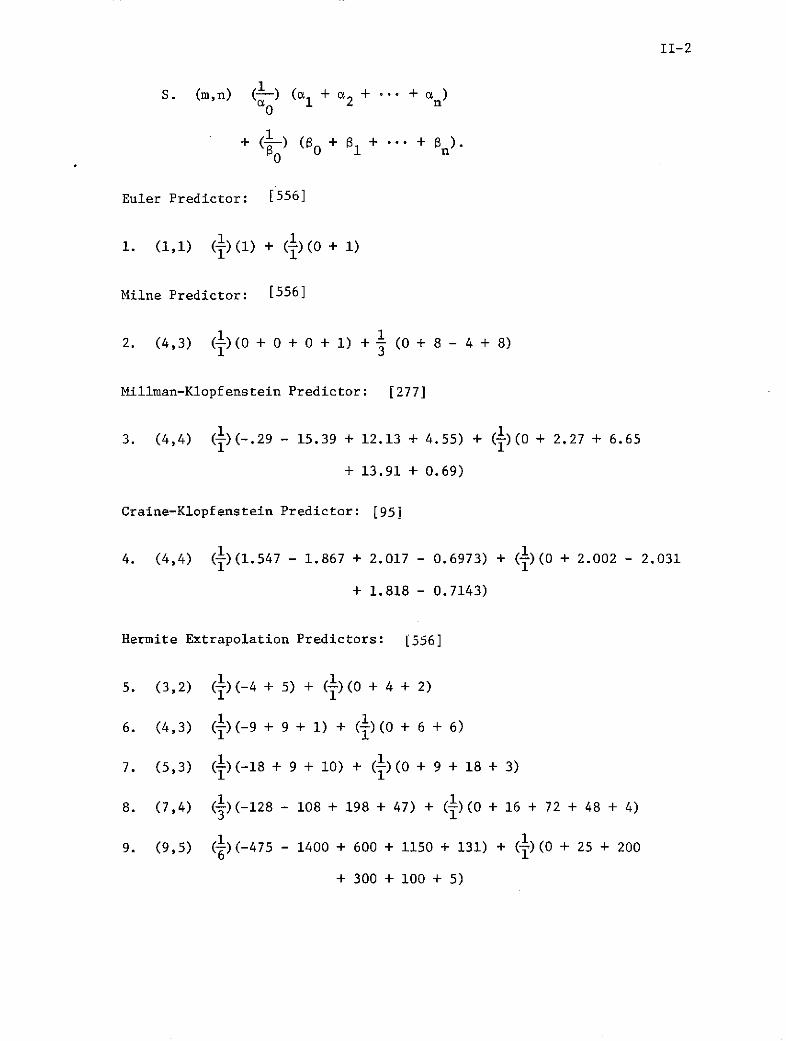
II-2
S. (m,n) (al + c2 + + a)a 0 1 2 n
+ ( ) ( 0 +1 + + n).0
Euler Predictor: [556]
1. (1,1) ( l)() + ()(0 + 1)
Milne Predictor: [556]
2. (4,3) (-)(0 + 0 + 0 + 1) + 1 (0 + 8 - 4 + 8)
Millman-Klopfenstein Predictor: [277]
3. (4,4) (-)(-.29 - 15.39 + 12.13 + 4.55) + (-)(0 + 2.27 + 6.65
+ 13.91 + 0.69)
Craine-Klopfenstein Predictor: [95]
4. (4,4) (-)(1.547 - 1.867 + 2.017 - 0.6973) + (-)(0 + 2.002 - 2.031
+ 1.818 - 0.7143)
Hermite Extrapolation Predictors: (556]
5. (3,2) )(-4 + 5) + ()(0 + 4 + 2)
6. (4,3) ()(-9 + 9 + 1) + ()(0 + 6 + 6)
7. (5,3) (I)(-18 + 9 + 10) + )(0 + 9 + 18 + 3)
8. (7,4) (-)(-128 - 108 + 198 + 47) + (j)(0 + 16 + 72 + 48 + 4)
119. (9,5) (-)(-475 - 1400 + 600 + 1150 + 131) + (-)(0 + 25 + 200
+ 300 + 100 + 5)
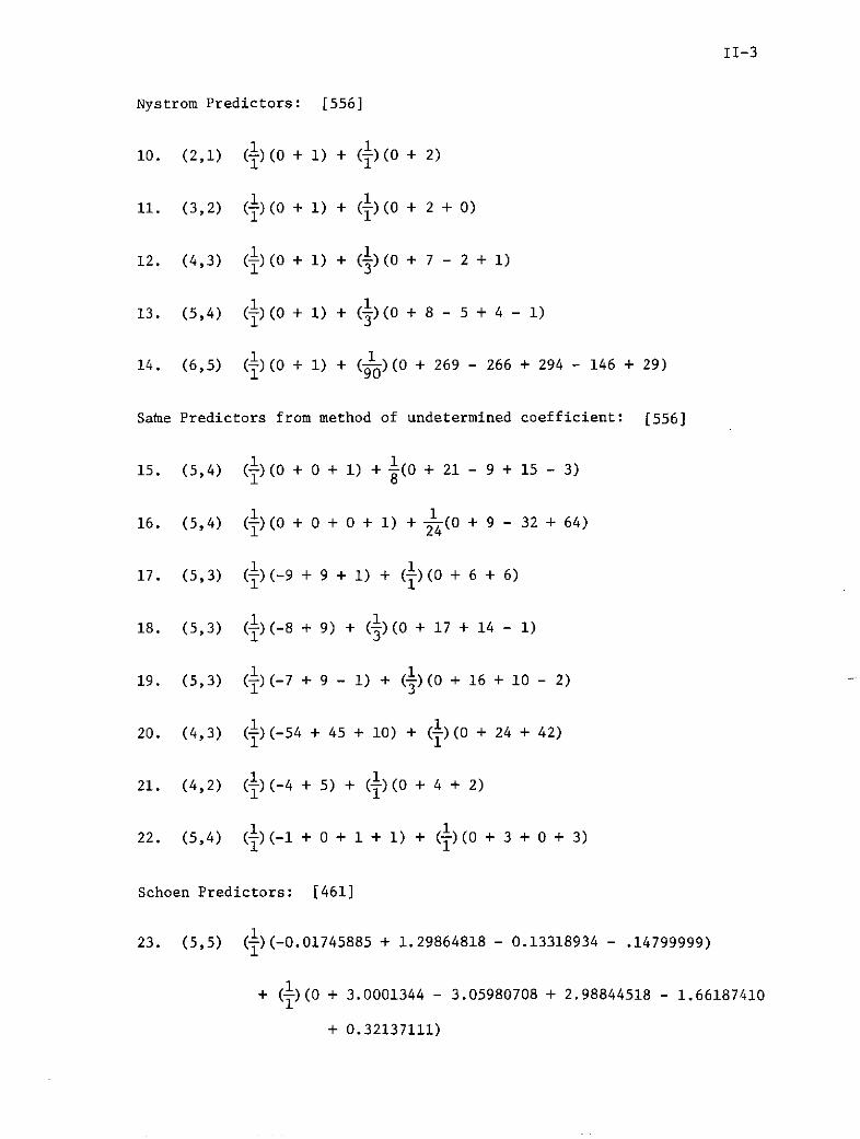
11-3
Nystrom Predictors: [556]
10. (2,1) (O)(0 + 1) + (')(0 + 2)
1 111. (3,2) ()(O + 1) + ()(0 + 2 + 0)
1 112. (4,3) (i)(0 + 1) + (1)(0 + 7 - 2 + 1)
13. (5,4) ( )(0 + 1) + (-)(0 + 8 - 5 + 4 - 1)
1 114. (6,5) (j)(0 + 1) + (-0)(0 + 269 - 266 + 294 - 146 + 29)
Same Predictors from method of undetermined coefficient: [556]
15. (5,4) (1)(0 + 0 + 1) + i(0 + 21 - 9 + 15 - 3)
1 116. (5,4) (i)(0 + 0 + 0 + 1) + 4(0 + 9 - 32 + 64)
17. (5,3) (-)(- 9 + 9 + 1) + (-)(0 + 6 + 6)
1 118. (5,3) (i)(-8 + 9) + (1)(0 + 17 + 14 - 1)
19. (5,3) (1)(-7 + 9 - 1) + (-)(0 + 16 + 10 - 2)
20. (4,3) ()(-54 + 45 + 10) + (j)(0 + 24 + 42)
1 121. (4,2) (i)(-4 + 5) + (i)(0 + 4 + 2)
1 122. (5,4) (1)(-l + 0 + 1 + 1) + ()(0 + 3 + 0 + 3)
Schoen Predictors: [461]
23. (5,5) (1)(-0.01745885 + 1.29864818 - 0.13318934 - .14799999)
+ (j)(0 + 3.0001344 - 3.05980708 + 2.98844518 - 1.66187410
+ 0.32137111)

11-4
24. (6,6) (i)(-.92790378 + 2.05094161 + .54664912 - 0.67100875
+ 0.0005296 + 0.00126884) + (1)(0 + 3.60328436
- 3.60284254 + 5.40345116 - 4.77344249 + 1.80481406
- 0.29749495)
Krough Predictors: [556]
25. (4,4)(A) (-)(1 + 1) + (8)(0 + 119 - 99 + 69 - 17)
1 126. (4,4)(B) (--)( 4 + 3) + (-2-)(O + 103 - 88 + 61 - 15)
1 127. (5,5) (- )(-1 + 32) + (-740-)(0 + 22,321 - 21,774 + 24,216
- 12,034 + 2391)
28. (6,6) 1 128. (6,6) (--)(-11 + 23) + (7 )(0 + 62,248 - 62,255 + 101,430
- 76,490 + 30,545 - 5079)
1 129. (7,7) (-O)(-21 + 31) + (604800) (0 + 2,578,907 - 2,454,408
+ 5,615,199 - 5,719,936 + 3,444,849 - 1,149,048
+ 164,117)
Adams-Bashforth Predictors: [556]
30. (2,2) (j)(1) + (-)(0 +3 - 1)
1 131. (3,3) (t)(1) + (--2)(0 + 23 - 16 + 5)
32. (4,4) (1i)(1) + (-)(O + 55 - 59 + 37 - 9)
33. (5,5) ()(1) + (-720)(0 + 1901 - 2774 + 2616 - 1274 + 251)
34. (6,6) ()(1) + (4--40) (0 + 4277 - 7923 + 9982 - 7298 + 2887 - 475)

11-5
35. (7,7) (1)(1) + 60,480)(0 + 198,721 - 447,288 + 705,549 - 688,256
+ 407,139 - 134,472 + 19,087)
36. (8,8) )(1) + (1201960)(0 + 434,241 - 1,162,169 + 2,183,877
- 2,664,477 + 2,102,243 - 1,041,723 + 295,767
- 36,799)
Milne Corrector: [556]
1 137. (4,2) (i)(0 + 1) + (i-)(1 + 4 + 1)
Hamming Corrector: [556]
38. (4,2) (-)(9 + 0 - 1) + (-)(3 + 6 - 3)
Milne-Reynolds Corrector: [361]
39. (5,3) (- )(1 + 7) + (19 2 )(65 + 243 + 51 + 1)
Correctors from method of undetermined coefficients: [556]
40. (4,2) (-)(4 + 1) + (i)(2 + 4)
41. (5,3) (j)(0 + 0 + 1) + ()(3 + 9 + 9 + 3)
1 142. (5,3) (-)(1 + 1 + 1) + (-6)(1 3 + 39 + 15 + 5)
1 143. (5,3) (- )(1 + 1) + (-8)(17 + 51 + 3 + 1)
1 144. (5,3) (-)(2 + 1) + (- -2)(25 + 91 + 43 + 9)
1 145. (5,3) (--)(9 + 9 - 1) + (7-)( 6 + 18)
46. (53)()(9 + - )+( 0 + 22 - 8)146. (5,3) (- )(9 + 1- 1) + (-f-)(10 + 22 - 8)
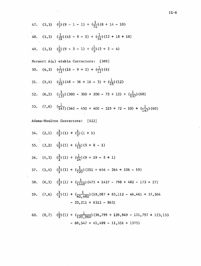
11-6
47. (5,3) (i)(9- 1 - 1) + (-1)(8 + 14 - 10)
48. (5,3) (-1)( 4 5 - 9 - 5) + (-i)(12 + 18 + 18)
49. (5,3) ()(9 - 3 - 1) + ()(2 + 2 -4)
Norsett A(a) stable Correctors: [389]
1 150. (4,3) (-)( 1 8 - 9 + 2) + (ft)(6)
1 151. (5,4) (-)(48 - 36 + 16 - 3) + (12)
52. (6,5) (-37-)( 3 0 0 - 300 + 200 - 75 + 12) + (y3-)(60)
53. (7,6) (' 147)(360 - 450 + 400 - 225 + 72 - 10) + (-147)(60)
Adams-Moulton Correctors: [422]
54. (2,1) (i)(1> + (-)(1 + 1)
55. (3,2) ()(1) + (f2)(5 + 8 - 1)
56. (4,3) (i)(1) + (--4)( 9 + 19 - 5 + 1)
1 157. (5,4) (-)(1) + (.2-)(251 + 646 - 264 + 106 - 19)
1 158. (6,5) (-)(1) + (- -)(475 + 1427 - 798 + 482 - 173 + 27)
1 1440
59. (7,6) (1)(1) + (60, 80)(19,087 + 65,112 - 46,461 + 37,504
- 20,211 + 6312 - 863)
60. (8,7) 1)(1) + (120960)(36,799 + 139,849 - 121,797 + 123,133
- 88,547 + 41,499 - 11,351 + 1375)
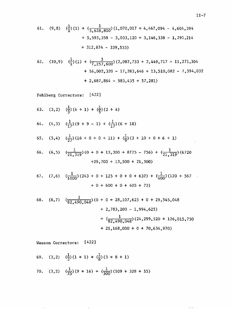
S1-7
61. (9,8) (1)() + (3,628,800)(1,070,017 + 4,467,094 - 4,604,594
+ 5,593,358 - 5,033,120 + 3,146,338 - 1,291,214
+ 312,874 - 339,533)
62. (10,9) (-)(1) + (7,251,600)(2,082,753 + 2,449,717 - 11,271,304
+ 16,002,320 - 17,283,646 + 13,510,082 - 7,394,032
+ 2,687,864 - 583,435 + 57,281)
Fehlberg Correctors: [422]
63. (3,2) )(4 + 1) + (t)(2 + 4)
1 164. (4,3) ()(9 + 9 - 1) + (T7)(6 + 18)
65. (5,4) (-7)(16 + 0 + 0 + 11) + (-)(3 + 10 + 0 + 6 + 1)
1 166. (6,5) (1)(0 + 0 + 13,300 + 8775 - 756) + (21,319-- (6720
21,319 21,319
+29,700 + 13,500 + 21,300)
1 167. (7,6) ( 1 )(2 4 3 + 0 + 125 + 0 + 0 + 632) + ( -)(120 + 567
+ 0 + 600 + 0 + 405 + 72)
68. (8,7) (2,49 48)(0 + 0 + 28,107,625 + 0 + 29,545,04882,490,048
+ 2,783,200 - 1,994,625)
+ ( 8 2 , 4 )(24 ,299 ,520 + 126,015,75082,490,048
+ 21,168,000 + 0 + 70,634,970)
Wesson Correctors: [422]
1 169. (3,2) (-)(1 + 1) + ( -)(3 + 8 + 1)
1 170. (3,2) (- -)(9 + 16) + (--.)(109 + 328 + 55)
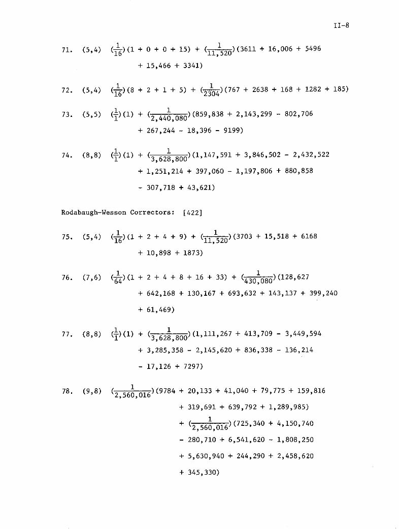
11-871. (5,4) ( )(1 + 0 + 0 + 15) + (11520(3611 + 16,006 + 5496
+ 15,466 + 3341)
1 172. (5,4) (-6)(8 + 2 + 1 + 5) + (--304)(767 + 2638 + 168 + 1282 + 185)
73. (5,5) ()(1) + (2,440,080)(859,838 + 2,143,299 - 802,706
+ 267,244 - 18,396 - 9199)
74. (8,8) ( )(1) + (3,628,800)(1,147,591 + 3,846,502 - 2,432,522
+ 1,251,214 + 397,060 - 1,197,806 + 880,858
- 307,718 + 43,621)
Rodabaugh-Wesson Correctors: [422]
75. (5,4) (- 6)(1 + 2 + 4 + 9) + (11,520)(3703 + 15,518 + 6168
+ 10,898 + 1873)
76. (7,6) (- )(1 + 2 + 4 + 8 + 16 + 33) + (4301080)(128,627
+ 642,168 + 130,167 + 693,632 + 143,137 + 399,240
+ 61,469)
1 177. (8,8) (i)(1) + (3,628,800)(1,111,267 + 413,709 - 3,449,594
+ 3,285,358 - 2,145,620 + 836,338 - 136,214
- 17,126 + 7297)
78. (9,8) (2,6, )(9784 + 20,133 + 41,040 + 79,775 + 159,8162,560,016
+ 319,691 + 639,792 + 1,289,985)
+ (2, 16)(725,340 + 4,150,740
- 280,710 + 6,541,620 - 1,808,250
+ 5,630,940 + 244,290 + 2,458,620
+ 345,330)