Embed Size (px)
Citation preview
Study of a Liquid-Vapour Ejector in the context of anadvanced TPL ejector-absorption cycle working with
a low temperature heat source and anammonia-water mixture
Filipe Alexandre Ereira Mendes Marques
Dissertação para a obtenção de Grau de Mestre em
Engenharia Física Tecnológica
Júri
Presidente: Doutor João Carlos Carvalho de Sá Seixas
Orientador: Doutor Luís Filipe Moreira Mendes
Vogais: Doutor Pedro José de Almeida Bicudo
Abril 2009

Agradecimentos
Agradeço ao meu Orientador e Professor Filipe Mendes pela oportunidade de realizar este trabalho,
por me apontar as fronteiras e quando devo parar, pela orientação, amizade e toda a experiência e
conhecimento partilhado.
Agradeço aos meus colegas e amigos do LSAS pelas ideias discutidas nas reuniões e partilha
de experiências, são eles o João Cardoso, o Igor, a Gisela, e em especial, agradeço ao Tiago Osório
por todo o paciente apoio e ajuda quando os programas teimavam em não correr.
Agradeço ao Coordenador de Curso Professor João Seixas por suavizar o processo burocrático
na transição para Mestrado de Bolonha, minimizando as minhas preocupações com o processo,
desviadas apenas para o trabalho.
Agradeço ao Professor Teixeira Borges a disponibilidade e dúvidas esclarecidas.
Agradeço ao Professor Felix Ziegler e ao Tobias Zegenhagen pelas interessantes discussões
acerca do meu trabalho.
Agradeço à Ana Gonçalves e ao Luís pela disponibilidade para ajuda no arranque do trabalho.
Agradeço o apoio e experiência partilhada de teses anteriores aos amigos Hugo Serôdio, Carlos
Afonso, Ana Roque, Luís Diogo e Catarina Simões.
Agradeço o apoio e paciência aos amigos/as Filipe, Francisca, João Carias, João Laia, Lia, Sara,
e felizmente muitos outros. . .
Finalmente, agradeço aos meus pais e irmão todo o apoio, ajuda e suporte durante a minha vida
académica.
i

Resumo
No âmbito deste trabalho, estudaram-se os limites da utilização de um ejector líquido-vapor sem
mudança de fase para recuperação de pressão, tendo em vista a sua colocação à entrada do
absorvedor num ciclo de absorção a funcionar com uma mistura de amoníaco-água e uma fonte
quente de baixa temperatura (p.ex. colector solar), convertendo-se num ciclo TPL por ejecção-
absorção.
De forma a encontrar a máxima recuperação de pressão possível e a respectiva geometria e pro-
priedades do ejector a funcionar sob determinadas condições no ciclo específico, foi desenvolvido e
aplicado sob a forma de um programa de simulação, um novo modelo teórico do fluxo bifásico num
ejector de líquido-vapor. O novo modelo procura expandir e ultrapassar as sobre-simplificações
encontradas nos modelos actualmente usados para simulação de ejectores. O modelo assume no
difusor que a fase líquida toma a forma de gotas e incluí a interacção entre as fases, efeitos inerci-
ais, acrescentando um termo para as perdas de pressão e dissipação de energia devidas à fricção
com as paredes, e tem em conta a composição da mistura binária de cada uma das duas fases, a
sua variação com a transferência de massa, assim como a variação do diâmetro das gotas.
Foi observada grande sensibilidade da pressão em relação a variações no diâmetro à saída do
pulverizador e proximidade à pressão correspondente ao início de mudança de fase.
Da simulação do ejector, observou-se que a recuperação de pressão aumenta para ângulos
menores do difusor, tendo-se encontrado um máximo de recuperação de 0,05 bar para um tubo,
observando-se que a recuperação de pressão se deve fundamentalmente à mistura dos fluidos.
Neste caso particular do uso duma mistura de amoníaco-água, verifica-se pois a necessidade
de estender o modelo para incluir mudança de fase no pulverizador de forma a tornar significativa a
recuperação de pressão.
Palavras-chave:Ejector; Injector; Bomba de Jacto; Máquina de Absorção; Ciclos TPL; Ciclos ejector-absorção; Pul-
verizador; Difusor; Amoníaco-Água
iii

Abstract
In this work, the limits of the use of a liquid-vapour ejector without phase change were studied for
pressure recovery, in view of its introduction at the absorber inlet, in a single-stage absorption cycle
working with a low temperature heat source and an ammonia-water mixture, therefore converting
the cycle into an advanced TPL ejector-absorption cycle.
In order to find the possible pressure recovery and respective ejector design, within the desired
cycle’s working conditions, a new two-phase flow model for the liquid-vapour ejector was developed
and applied as a simulation program. The model aims to expand the currently used models. It as-
sumes the liquid phase in the form of droplets in the conical diffuser and includes interaction between
phases, inertial effects and adds pressure losses due to friction, the binary mixture composition of
ammonia-water for each phase and its variation with mass transfer, as well as the droplets diameter
variation.
From the simulation of the mixing zone and the diffuser, it was found that the pressure recovery
increases for lower diffuser angles, with a maximum pressure recovery of 0,05 bar for a tube, observ-
ing that the pressure recovery is fundamentally due to the mixture of the fluids. An high sensibility of
the nozzle’s outlet pressure with the diameter variation was observed and analysed.
In this specific case of the use of ammonia-water as the working mixture, it was found the need
to expand the ejector’s model to include phase change at the nozzle, in order to have significant
pressure recover.
Key-words:Ejector; jet pump; Injector; Nozzle; Diffuser; Absorption machine; TPL cycle; ejector-absorption
cycle;ammonia-water
v

Contents
Resumo iii
Abstract v
List of Tables ix
List of Figures x
1 Introduction 1
2 Ejector’s History and State of the Art 7
2.1 History of the Injector/Ejector . . . . . . . . . . . . . . . . . . . . . . . . . . . . . . . . 7
2.2 Literature Review . . . . . . . . . . . . . . . . . . . . . . . . . . . . . . . . . . . . . . . 9
3 Model of the Ejector 15
3.1 Introduction to the Ejector . . . . . . . . . . . . . . . . . . . . . . . . . . . . . . . . . . 15
3.2 Injector . . . . . . . . . . . . . . . . . . . . . . . . . . . . . . . . . . . . . . . . . . . . 17
Nomenclature . . . . . . . . . . . . . . . . . . . . . . . . . . . . . . . . . . . . . 18
3.2.1 Model . . . . . . . . . . . . . . . . . . . . . . . . . . . . . . . . . . . . . . . . . 19
3.2.2 Interior Nozzle . . . . . . . . . . . . . . . . . . . . . . . . . . . . . . . . . . . . 21
3.2.3 Affected fluid entry . . . . . . . . . . . . . . . . . . . . . . . . . . . . . . . . . . 28
3.3 Diffuser . . . . . . . . . . . . . . . . . . . . . . . . . . . . . . . . . . . . . . . . . . . . 29
Nomenclature . . . . . . . . . . . . . . . . . . . . . . . . . . . . . . . . . . . . . 30
3.3.1 Multiphase Flow Notation and basic Definitions and Relations . . . . . . . . . . 31
3.3.2 Model . . . . . . . . . . . . . . . . . . . . . . . . . . . . . . . . . . . . . . . . . 35
3.3.3 Conservation Equations . . . . . . . . . . . . . . . . . . . . . . . . . . . . . . . 38
3.3.4 Interaction between the phases . . . . . . . . . . . . . . . . . . . . . . . . . . . 47
Nomenclature . . . . . . . . . . . . . . . . . . . . . . . . . . . . . . . . . . . . . 48
3.3.5 Droplet Diameter variation . . . . . . . . . . . . . . . . . . . . . . . . . . . . . . 56
4 Method of Simulation 57
4.1 Design Working Conditions . . . . . . . . . . . . . . . . . . . . . . . . . . . . . . . . . 59
5 Results and Discussion of the Simulations 61
5.1 Nozzle . . . . . . . . . . . . . . . . . . . . . . . . . . . . . . . . . . . . . . . . . . . . . 61
5.2 Diffuser . . . . . . . . . . . . . . . . . . . . . . . . . . . . . . . . . . . . . . . . . . . . 64
5.2.1 Simple Diffuser . . . . . . . . . . . . . . . . . . . . . . . . . . . . . . . . . . . . 64
vii
5.2.2 Two-Phase Diffuser . . . . . . . . . . . . . . . . . . . . . . . . . . . . . . . . . 66
6 Conclusions 71
A Formulae development 77A.1 Ejector Surface: solid surface projection . . . . . . . . . . . . . . . . . . . . . . . . . . 77
A.2 Injector Surface Force: Nozzle’s total surface force . . . . . . . . . . . . . . . . . . . . 78
A.3 Nozzle’s mechanical energy loss . . . . . . . . . . . . . . . . . . . . . . . . . . . . . . 79
A.4 Fluid Conservation Equations with Interaction . . . . . . . . . . . . . . . . . . . . . . . 81
A.4.1 Conservation of Mass . . . . . . . . . . . . . . . . . . . . . . . . . . . . . . . . 82
A.4.2 Conservation of Ammonia’s Mass . . . . . . . . . . . . . . . . . . . . . . . . . 82
A.4.3 Conservation of the Momentum . . . . . . . . . . . . . . . . . . . . . . . . . . . 83
A.4.4 Conservation of Energy . . . . . . . . . . . . . . . . . . . . . . . . . . . . . . . 84
A.5 Droplet Volume Change with Mass transfer . . . . . . . . . . . . . . . . . . . . . . . . 85
B Simulation Program Formatted Code 87
viii
List of Tables
4.1 Geometrical Initial Conditions . . . . . . . . . . . . . . . . . . . . . . . . . . . . . . . . 59
4.2 Initial conditions of the motive flow (weak solution). . . . . . . . . . . . . . . . . . . . . 60
4.3 Initial conditions of the affected flow (refrigerant). . . . . . . . . . . . . . . . . . . . . . 60
5.1 Simple Vapour Diffuser . . . . . . . . . . . . . . . . . . . . . . . . . . . . . . . . . . . 65
ix
List of Figures
1.1 Triple-pressure-level single-stage advanced absorption cycle. . . . . . . . . . . . . . . 2
1.2 4 effects by the TPL cycle . . . . . . . . . . . . . . . . . . . . . . . . . . . . . . . . . . 4
3.1 Ejector . . . . . . . . . . . . . . . . . . . . . . . . . . . . . . . . . . . . . . . . . . . . . 16
3.2 Longitudinal section of the injector. . . . . . . . . . . . . . . . . . . . . . . . . . . . . . 19
3.3 Section of a nozzle with a quasi-one-dimensional flow. . . . . . . . . . . . . . . . . . . 19
3.4 Control Volume for the Nozzle. . . . . . . . . . . . . . . . . . . . . . . . . . . . . . . . 21
3.5 Differential incremental control volume. . . . . . . . . . . . . . . . . . . . . . . . . . . 25
3.6 Element of surface, showing the normal and parallel unit vector. . . . . . . . . . . . . . 26
3.7 A longitudinal section of the Injector: the affected fluid entry. . . . . . . . . . . . . . . . 28
3.8 Diffuser’s volume element for the flow. . . . . . . . . . . . . . . . . . . . . . . . . . . . 36
3.9 Diffuser’s infinitesimal control volume. . . . . . . . . . . . . . . . . . . . . . . . . . . . 36
3.10 Diffuser’s longitudinal section. . . . . . . . . . . . . . . . . . . . . . . . . . . . . . . . . 38
5.1 P(D) in the interior nozzle. . . . . . . . . . . . . . . . . . . . . . . . . . . . . . . . . . . 62
5.2 u(D) in the interior nozzle. . . . . . . . . . . . . . . . . . . . . . . . . . . . . . . . . . . 63
5.3 Simple Vapour Diffuser. ∆P (D) . . . . . . . . . . . . . . . . . . . . . . . . . . . . . . . 65
5.4 ∆P (ρv,outlet) (estimate) . . . . . . . . . . . . . . . . . . . . . . . . . . . . . . . . . . . 67
5.5 ∆ P(y) in the Diffuser. . . . . . . . . . . . . . . . . . . . . . . . . . . . . . . . . . . . . 69
5.6 u(y) (20cm diffuser) . . . . . . . . . . . . . . . . . . . . . . . . . . . . . . . . . . . . . 70
A.1 The surface of a cone: parameters for area calculation. . . . . . . . . . . . . . . . . . 77
A.2 Element of surface, with the normal and parallel unit vector. . . . . . . . . . . . . . . . 78
A.3 Pressure on the nozzle’s wall. Note: the arrows dimensions illustrate the interior
pressure variation along the solid surface, but not necessarily the difference of the
magnitude related to the exterior pressure (atmospheric). . . . . . . . . . . . . . . . . 78
x
Chapter 1
Introduction
In sunny and warm countries like Portugal, one of the highest energy spending is on air conditioning
and coolers during spring, summer and begins of autumn [1]. Absorption cooling technologies driven
by thermal solar energy come up as promising alternatives to the conventional intensive electrical
energy spending cooling technology.
One characteristic greatly responsible for slowing up the progress into market of absorption tech-
nologies is its lower efficiency compared to conventional technologies, which implies the use of large
solar fractions in order to have comparable fossil primary energy consumption, i.e., comparable CO2
emissions [2]. Advanced absorption cycles are being studied in order to increase the Coefficient of
Performance (COP) of this type of machines, as well as its adaptability and to widen the scope of its
uses [3], [4].
In this chapter, the context of the present work will be introduced. It is assumed that the reader
is already familiarized with Absorption Chillers [5].
In spite of that, the following chapters might be of interest for a reader searching for the theory
and simulation of the ejector/injector without regarding this particular application, object of this work.
One type of such advanced cycles is the Triple Pressure Level cycle (TPL), which consist of the
conventional Double Pressure Level cycle (DPL) with an extra intermediate pressure level, achieved
by means of a pump or pump like device.
A jet pump or Ejector seems to be a very good solution to maintain the pressure difference,
because it has no moving parts, requires low maintenance, do not need an additional energy source,
as it uses energy otherwise lost in the cycle, and it is cost effective. A TPL cycle by means of an
ejector is called an advanced ejector-absorption cycle.
As referenced in the literature review, in chapter 2.2, the ejector may be applied in different ways
in simple or more complex absorption cycles.
The present work is engaged in the context of a single-stage absorption refrigeration cycle, with
a binary mixture of ammonia-water as the working fluid and a low temperature heat input. The
motivation for the present work is to convert the existing DPL single-stage absorption refrigeration
cycle, applied in a Lab prototype chiller at the LSAS 1 in IST, into a TPL ejector-absorption cycle,
in view of decreasing the generator temperature while maintaining or increasing the COP and thus,
1Laboratorio de Sistemas de Arrefecimento Solar
1
obtaining higher solar fractions.
A TPL advanced absorption cycle derived from a single-stage absorption cycle, is usually ob-
tained by introducing [3], [4]:
• a specifically designed vapour-vapour ejector at the condenser inlet, adding a triple valve at
the evaporator’s outlet, for suction of the refrigerant and evaporation improvement.
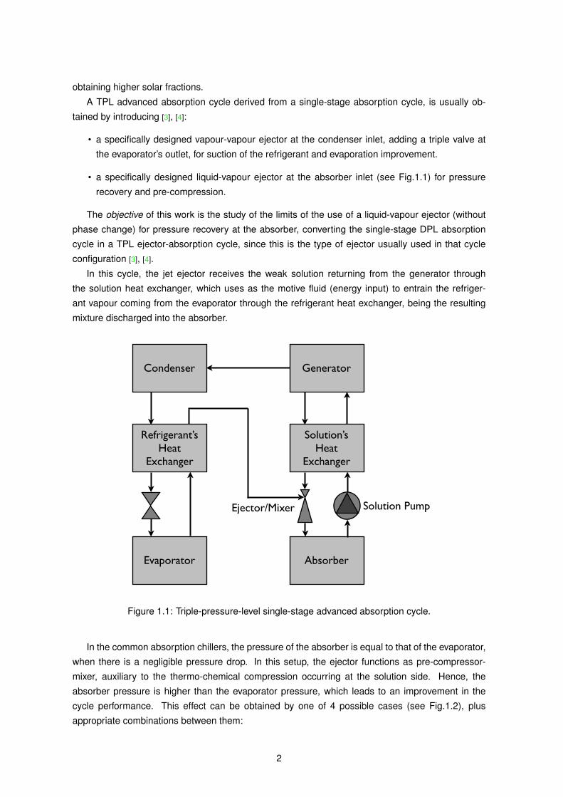
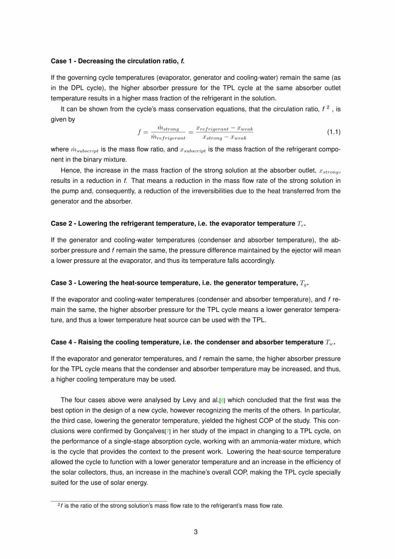
• a specifically designed liquid-vapour ejector at the absorber inlet (see Fig.1.1) for pressure
recovery and pre-compression.
The objective of this work is the study of the limits of the use of a liquid-vapour ejector (without
phase change) for pressure recovery at the absorber, converting the single-stage DPL absorption
cycle in a TPL ejector-absorption cycle, since this is the type of ejector usually used in that cycle
configuration [3], [4].
In this cycle, the jet ejector receives the weak solution returning from the generator through
the solution heat exchanger, which uses as the motive fluid (energy input) to entrain the refriger-
ant vapour coming from the evaporator through the refrigerant heat exchanger, being the resulting
mixture discharged into the absorber.
������������������
���������� ��������
��������������
���������
�����������������
���������
��������������������������
Figure 1.1: Triple-pressure-level single-stage advanced absorption cycle.
In the common absorption chillers, the pressure of the absorber is equal to that of the evaporator,
when there is a negligible pressure drop. In this setup, the ejector functions as pre-compressor-
mixer, auxiliary to the thermo-chemical compression occurring at the solution side. Hence, the
absorber pressure is higher than the evaporator pressure, which leads to an improvement in the
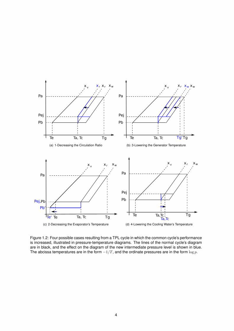
cycle performance. This effect can be obtained by one of 4 possible cases (see Fig.1.2), plus
appropriate combinations between them:
2
Case 1 - Decreasing the circulation ratio, f.
If the governing cycle temperatures (evaporator, generator and cooling-water) remain the same (as
in the DPL cycle), the higher absorber pressure for the TPL cycle at the same absorber outlet
temperature results in a higher mass fraction of the refrigerant in the solution.
It can be shown from the cycle’s mass conservation equations, that the circulation ratio, f 2 , is
given by
f =mstrong
mrefrigerant=xrefrigerant − xweakxstrong − xweak
(1.1)
where msubscript is the mass flow ratio, and xsubscript is the mass fraction of the refrigerant compo-
nent in the binary mixture.
Hence, the increase in the mass fraction of the strong solution at the absorber outlet, xstrong,
results in a reduction in f. That means a reduction in the mass flow rate of the strong solution in
the pump and, consequently, a reduction of the irreversibilities due to the heat transferred from the
generator and the absorber.
Case 2 - Lowering the refrigerant temperature, i.e. the evaporator temperature Te.
If the generator and cooling-water temperatures (condenser and absorber temperature), the ab-
sorber pressure and f remain the same, the pressure difference maintained by the ejector will mean
a lower pressure at the evaporator, and thus its temperature falls accordingly.
Case 3 - Lowering the heat-source temperature, i.e. the generator temperature, Tg.
If the evaporator and cooling-water temperatures (condenser and absorber temperature), and f re-
main the same, the higher absorber pressure for the TPL cycle means a lower generator tempera-
ture, and thus a lower temperature heat source can be used with the TPL.
Case 4 - Raising the cooling temperature, i.e. the condenser and absorber temperature Tw.
If the evaporator and generator temperatures, and f remain the same, the higher absorber pressure
for the TPL cycle means that the condenser and absorber temperature may be increased, and thus,
a higher cooling temperature may be used.
The four cases above were analysed by Levy and al.[6] which concluded that the first was the
best option in the design of a new cycle, however recognizing the merits of the others. In particular,
the third case, lowering the generator temperature, yielded the highest COP of the study. This con-
clusions were confirmed by Gonçalves[7] in her study of the impact in changing to a TPL cycle, on
the performance of a single-stage absorption cycle, working with an ammonia-water mixture, which
is the cycle that provides the context to the present work. Lowering the heat-source temperature
allowed the cycle to function with a lower generator temperature and an increase in the efficiency of
the solar collectors, thus, an increase in the machine’s overall COP, making the TPL cycle specially
suited for the use of solar energy.
2f is the ratio of the strong solution’s mass flow rate to the refrigerant’s mass flow rate.
3
Pa
Pb
Te Ta, Tc Tg
xv xr xw
Pej
xr
(a) 1-Decreasing the Circulation Ratio
Pa
Pb
Te Ta, Tc Tg
xv xr xw
Pej
xw
Tg'
(b) 3-Lowering the Generator Temperature
Pa
Pb
Te Ta, Tc Tg
xv xr xw
Pej,
Te'
Pb'
(c) 2-Decreasing the Evaporator’s Temperature
Pa
Pb
Te Ta,Tc Tg
xv xr xw
Pej
Ta,Tc
(d) 4-Lowering the Cooling Water’s Temperature
Figure 1.2: Four possible cases resulting from a TPL cycle in which the common cycle’s performanceis increased, illustrated in pressure-temperature diagrams. The lines of the normal cycle’s diagramare in black, and the effect on the diagram of the new intermediate pressure level is shown in blue.The abcissa temperatures are in the form −1/T , and the ordinate pressures are in the form log p.
4
In view of changing the current single-stage DPL absorption chiller (working with a low tempera-
ture heat source and an ammonia-water mixture) into a TPL ejector-absorption chiller in the future,
two questions arise:
• What is the pressure recovery possible by a liquid-vapour ejector working within the current
machine’s working conditions?
• What are the design conditions for the ejector?
In order to an answer this questions, this work proposes a new two-phase flow model for the
ejector. The model aims to expand the currently used two-phase subsonic ejector models described
in the literature review. It assumes the liquid phase in the form of droplets in the conical diffuser
and includes interaction between phases (mass, momentum and energy), inertial effects and adds
pressure losses due to friction, the binary mixture composition of ammonia-water for each phase
and its variation with mass transfer, as well as the droplets diameter variation.
A simulation program is then created based on the ejector’s model. The program is then used to
study the pressure recovery possible for an ejector working in an ejector-absorption cycle with low
temperature heat source and a binary mixture of ammonia-water, adding simulation results for this
specific type of ejector-absorption cycles (see literature review). Specifically, the cycle’s working and
design conditions used in this study, which provide a sample for the usual conditions of this type of
cycles, are the ones correspondent to the existing prototype chiller at the LSAS, from which we want
to know the potential for changing the current cycle into a TPL cycle in future works.
Outline of subsequent chapters
In chapter 2, an introduction to the ejector device, from a historical perspective is given, and then
the state of the art is reviewed.
In chapter 3, the model of the ejector is developed. Starts with an introduction to the ejector basics.
Next, the theoretical model for the injector is developed and discussed. After, the theoretical model
for the diffuser is developed and discussed. Starts with a notation and basic definitions introduction,
follows with the model development and discussion, and ends presenting the interaction terms and
droplet diameter variation.
In chapter 4, the method of simulation is presented, as well as the design working conditions for the
cycle.
In chapter 5, the results of the simulations are presented and discussed.
In chapter 6, conclusions are drawn and future paths for investigation are suggested.
5

6
Chapter 2
Ejector’s History and State of the Art
2.1 History of the Injector/Ejector
The Injector was invented by Henri Jacques Giffard, an eminent French mathematician and engineer,
for feeding boilers, utilizing in a novel and ingenious way the latent power of a discharging jet of steam
to suck and entrain the water from a reservoir and inject it into the boiler.
After his graduation from L’École Centrale in 1849, Giffard devoted his time to the study of aero-
nautics and, in particular, to the development of a light steam motor for propelling balloons. In the
process he devised a compact and convenient substitute for the steam pumps then in use. On May
8, 1858, letters patent were issued for L’Injecteur Automoteur.
Theoretically, the method by which Giffard proposed to force a continuous stream of water into
the boiler appeared to be entirely feasible and would have, if practicable, many advantages over
the intermittent systems. The difficulty seemed to lie in fulfilling the peculiar conditions required for
the condensation of the steam and the subsequent reduction of the velocity of the moving mass.
The various phases of the question were carefully considered, and he made a working drawing
embodying his ideas. A model was made by M.Flaud & Cie., of Paris, who found, however, consid-
erable difficulty in forming the tubes in the peculiar shapes required. In the shape and proportions
of the nozzles lay the element of success, and the first instrument constructed entirely fulfilled the
expectation of the designer.[8]
In 1860 he published a small brochure entitled "A Theoretical and Practical Paper on the Self-
acting Injector", where he points out the advantages in using the injector instead of the usual appa-
ratus employed for feeding water to the boiler, describes his invention in detail and explains the best
proportions for its various parts, and also the mechanical theory, substantially as advanced by him
in 1850, eight years before the construction of his experimental Injector.
Great difficulty was first experienced by the injector in obtaining a fair trial of its merits, possibly
due to the mystery that seemed to surround its working, and the general skepticism as to its practical
anti-wearing capacity. However, the advantages of this method over the old ones were so numerous
and apparent, that it was speedily recognized and introduced everywhere when steam was used as
a motive power. Such appreciation by the Academie des Sciences of France awarded Giffard the
Grand Mechanical Prize for 1859.
The advantages previewed and learned from experience include: continuous injection; enhances
the safety of those who approach the boiler; compact; it requires less attention on the part of the
operator, as the best injectors are self-adjusting and fulfill their requirements under all conditons
of duty, being at the same time less liable to get out of order, and not requiring consequently so
7
frequent and so expensive repairs, as the ordinary pump does. By using the injector no difficulty is
experienced in adjusting the openings for steam and water, so as to produce a constant and regular
supply of any required quantity of water to the boiler without waste from the overflow, while the feed,
at the same time, may be varied sufficiently to meet the varying demand.[9]
The action of a fluid issuing from an orifice with great velocity, and carrying along with it another
fluid or semi-fluid with which contacts on its route, was known up to 1570, when Vitrio and Philebert
de Lorme were using a crude ejecting apparatus. And there are reasons for supposing that it was
understood much earlier, because every man in forcing a strong current of air through the cavity of
his nose, for the purpose of getting rid of the secretion which has accumulated inside of his nostrils,
utilizes this principle of injector and uses it as an ejector.
The first device that bears any similarity to the principle of the Injector was patented August
15,1818, by Mannoury de Dectot, who describes "sundry motors or means for employing the power
of fire, of steam, of air, etc., to start the movement of machines." He applied his invention for raising
water and for propelling boats by using the expansion and condensation of steam in connection with
jets of water. Ravard followed in 1840 with improved forms, but the greatest advance was made by
Bourdon, who approached very near the results obtained by Giffard (patent issued in 1857). This
contained numerous combinations of convergent and divergent tubes for transforming the energy of
a moving jet, or for discharging large or small quantities of liquid or gases. The similarity of the form
of the apparatus to that of Giffard was so marked that the question of priority at once arose and was
exhaustively discussed by the "Sociètè des Ingènieurs Civils". It was shown that Giffard was wholly
unaware of the last improvements of Bourdon when he applied for his patent, and as he had publicly
presented the theory of his invention nearly seven years in advance of Bourdon, full credit was given
him for the conception of the Injector and originality in the application of the principle.
The Injector was introduced into England by Sharp, Steward & Co., of Manchester, in 1859. At
about the same time, the Paris representative of Messrs. Robert Stephenson & Co., Newcastle, sent
over to them a similar Injector, however, they were unlucky to couple it up incorrectly. The English
railroads opened a wide field for the Injector.
The Injector was introduced in the United States by Messrs. Wm. Sellers & Co., who started its
manufacture in 1860 at their works in Philadelphia, with very important improvements.
In Europe Giffard’s injector was subjected to a series of very important modifications in the hands
of Del-Peche, Kraus, Korting, Friedmann, and others. The improvements consisted mainly in the
more judicious arrangement of parts of the apparatus, and in replacing others by new attachments,
which increased the effectiveness and facilitated its operation. Amongst the American inventions
may be mentioned the Hancock’s, Rue’s, Desmond’s, Penberthy’s, Murdock’s, and Eberman’s.[9]
In the year 1910, owing to improvements introduced, American Injectors were extensively used
even in France, and were adopted as a standard type by several of the government’s railroads in the
country of its inventor.
The Injector was since applied to numerous other purposes. The capacity of the liquified jet of
carrying along with it double of its own volume of water with a comparatively speaking small loss of its
own velocity, made it useful for fire extinguishing purposes. The steam coming from the boiler carried
along the water to a greater height, than it could rise itself without this assistance. Other uses of the
injector include: injection of chemicals into small boilers; in thermal power stations, they are used
for the removal of the boiler bottom ash, the removal of fly ash from the hoppers of the electrostatic
precipitators used to remove that ash from the boiler flue gas, and for creating vacuum pressure in
8
steam turbine exhaust condensers; in producing vacuum pressure in steam jet cooling systems; for
the bulk handling of grains or other granular or powdered materials; the construction industry uses
them for pumping turbid water and slurries; laboratories use it to create a partial vacuum and for
medical use in suction of mucus or bodily fluids.
There is an implicit equivalence between the original designation Injector and the designation
Ejector : "Every injector, in the first place, is necessarily an ejector, for the same reason that every
feed pump is at the same time a draw out or exhaust pump, because in pumping into one receiver it
must pump out its stuff from some other one. The special object in view, it is true, modifies in each
case the construction of the apparatus, but the principle remains one and the same." [9]
For the purposes of this work, the component will be called Ejector, and the piece of the compo-
nent that injects the working fluids into the ejector will be called Injector.
2.2 Literature Review
As stated before in chapter 2.1, the invention of the ejector is old and numerous studies have been
made to perfect the apparatus, mainly of practical/experimental nature, in search of more efficiency,
along with the appearance of new uses. The theory and experimental input keeps developing syn-
chronized with the development of the fields of Fluid Mechanics and Energy, Mass, and Momentum
Transfer.
The use of ejectors with absorption machines is recent. A patent by Kuhlenschmidt [12] was
published in 1973 that is believed to be the first official record of the application of an ejector to an
absorption chiller. The patent for an air-cooled double-effect salt solution absorption refrigeration
machine having high and low pressure generator stages and operated with a lower pressure in
the evaporator than in the absorber, mentions an ejector which acts as a compressor between
the evaporator and the absorber and employs refrigerant vapor flowing from the lower pressure
generator stage as the driving fluid. The new cycle achieved the desired low evaporator temperature
while permitting the absorber to use an absorbent salt solution having a lower salt concentration and
hence lower crystallization temperature with the same cooling effect, not improving the machine’s
COP.
The use of an ejector as a jet-pump to recover pressure, gave birth to a new type of cycles,
the ejector-absorber cycles, which are included in a new type of cycles called Triple Pressure Level
cycles (TPL), a branch of the Advanced Absorption Cycles.
In 1983, an article by Chung et al [13] was published (in the context of an international confer-
ence), which is believed to be the first article on the subject of the application of an ejector to an
absorption cycle. In 1988, L.Chen[14] presents an analysis of a modified ejector-absorber absorp-
tion refrigeration cycle, using R-22/DME-TEG as the working fluids. In both this articles, the cycle
presented use the returning solution from the generator as the motive fluid to entrain the refriger-
ant vapour from the evaporator, being the resulting mixture discharged into the absorber 1 . The
model for the ejector presented by Chen uses a Bernoulli type equation to model the two phase
flow through the ejector, which was based in a single-phase flow model of a pseudo-fluid, thus not
taking into account the phases interactions and losses 2 . Results for a system with a 0,85 diffuser
efficiency are computed, and a considerable improvement in COP is observed.
1in [3]2in [15]
9
In 1994, a more detailed numerical model of the jet-ejector and its analysis, having in view the
design of the device for future incorporation in an absorption machine, was published. N.Daltrophe,
M.Jelinek and I.Borde ([16], [17])) describe a numerical model of non-isothermal simultaneous mass,
heat, and momentum transfer between the gas phase and the liquid phase in the diffuser which also
functions as the mixing chamber. Importance is given to the process of mixing and pre-absorption in
the ejector, to the detriment of pressure recovery. The model assumes an adiabatic unidimensional
steady flow, where the liquid phase is a binary mixture, and the gravitational and surface tension
forces are negligible. However it assumes also that the momentum transfer by friction with the
wall is negligible, only the liquid phase is a binary mixture and a constant droplet diameter. In this
present work, this model is to be expanded in order to overcome those assumptions. Calculations
were performed for a mixture of R134a and an organic absorbent. The simulation reveals that small
angles for the diffuser’s cone, with higher disperse phase velocities relative to the gas, yield higher
pressure recover, up to 0,5 bar (for organic ).
In 1998, Aphornratana et al.[18] describe the experimental study of a combined ejector-absorption
refrigeration cycle with the ejector placed between the generator and the condenser of a conventional
single-effect absorption refrigerator. The motive fluid used was the high pressure vapour refrigerant
produced in the generator, which entrained low pressure refrigerant vapour from the evaporator and
discharged it into the condenser, in order to enhance the evaporation process in this new ejector-
absorption cycle. The system used an aqueous lithium bromide solution, LiBr-water, as the working
fluid, and was tested with the generator pressure ranging from 1,98 to 2,7 bar, and the evaporator
temperature from 5 to 10 ◦C. The experimental results published present an increase of the cooling
capacity by up to 60% and coefficients of performance (COP) of 0,57 to 0,65 were found which was
a 25% increase over the single-effect absorption cycle (DPL cycle). However, the system required
a heat source temperature between 190 and 210 ◦C and relatively low-temperature cooling water
for the condenser and absorber. Earlier studies on this new cycle are reported in [3], that concern
the first experimental work on ejector-absorption cycles, which include Aphornratana’s phd thesis
(1994) on the subject[19], and the investigation by Eames et al. [20] published in the context of the
CIBSE National Conference (UK). It was reported [19] a measured COP in the range between 0,8 to
1,04 for 5 ◦C cooling temperature, provided a generator temperature of at least 200 ◦C, which may
result in increased corrosion rates[21].
A computer simulation program was developed for this novel refrigeration cycle and used to
determine the performance of the system, by Sun et al. in 1996 [22]. The analysis to predict the per-
formance of an ejector design is based in a single-phase flow model like the one used by Chen[14],
in particular, it was used the constant pressure mixing model which relies in the simplifying assump-
tions that: both fluids have the same molecular weight and ratio of specific heats; both streams are
supplied at zero velocities (i.e. stagnation conditions); both fluids mix at the nozzle’s exit at a uni-
form pressure across the section; transverse shocks might occur at any plane of the constant section
mixing zone; at the diffuser exit, the velocity is zero (i.e. stagnation conditions). The performance
of this cycle revealed to be superior to that of a common absorption machine. Optimum operating
conditions and data for optimum design of the ejector for the combined cycle were provided. This
cycle works with only one phase, the vapour, and the ejector was modeled with the commonly used
one phase model[23]. This is the most popular approach when dealing with ejectors. However, this
model requires assumptions that are not valid for two-phase flow models, and more complex models
are necessary as the one referred previously. I would like to give a particular emphasis to the as-
10
sumptions of stagnation conditions at the inlet and constant pressure mixing zone that are overcame
by the model developed in this present work and whose simulation results may help giving further
insight into the validity of such assumptions.
Wu et al.[3] reports also that a double ejector hybrid cycle, a combination of the cycles of Chung
et al.[13], Chen [14] and Eames et al. [20], was suggested by Gu et al. [24] (1996). The two ejectors
were used to entrain the refrigerant vapour from the evaporator: one whose motive fluid is the
returning solution from the generator and another driven by the refrigerant vapour from the generator,
with R21-DMF as working pairs. It was presented a calculated COP of 0,651 for this cycle. No
experimental results were provided.
Wu and Eames [25], [26] (1998) reported a novel ejector boosted single-effect absorption-recompression
refrigeration cycle, where a steam generator, ejector and a concentrator replace the high and low
pressure generators (concentrators) used in conventional double-effect absorption cycle machines,
to re-concentrate the absorbent solution. Here, the ejector acts like a heat-pump to enhance the
concentration process by increasing the flow of leaving vapour from the concentrator and compress-
ing it to such a state that it could be used as a heat input at the concentrator, re-heating the solution
from which it came. Calculations show a large dependence of the COP’s improvement towards the
performance of the steam ejector, obtaining results of 1,035, up to 1,2 with a better ejector design.
To drive this cycle, a high temperature heat source is required. This new refrigeration cycle was
developed having in mind the advantages of simple and low initial cost, as well as maintenance cost,
compared with the double-effect absorption cycle, achieving a similar COP.
Wang et al.[27] (1998) describes and study a solar-driven ejection absorption refrigeration (EAR)
cycle with reabsorption of the strong solution and pressure boost of the weak solution. It is concluded
that the EAR cycle has advantages over the conventional cycle, being adaptable to varying operating
conditions, especially in utilization of the low-grade unsteady heat sources like the solar energy.
Jelinek et al.[6] (2002) studied the influence of the jet ejector on the performance of the TPL
absorption cycle and compared it to that of the common double-pressure level (DPL) cycle. Four
cases were studied that exhibit advantages in cycle performance: the ability to reduce the circulation
ratio, the ability to lower the evaporator temperature, the ability to lower the generator temperature
and the ability to use higher-temperature cooling water. The working fluid used in the simulation
was R125-DMEU. The jet ejector at the absorber inlet, was used for pressure recovery and improve
the mixing between the weak solution and the refrigerant vapour coming from the evaporator. It
was concluded that the first case, to reduce the circulation ratio, was the best option in the design
of a new cycle, even so it was recognized the others have their own merits. Within the parametric
study, the best efficiency attained was a COP of 0,555 (5,3% improvement), when the generator
temperature was varied -11,3 ◦C (3rd case), followed by the 1st case which with a 20% reduction of
the circulation ratio to 3,27 attains a 4,6% increase in the COP. Pressure recovery up to 9% were
obtained. Results show a pressure recovery increasing with the temperature of the evaporator and
the decrease of the temperature in the generator. A COP of 0,595 was achieved when the evaporator
temperature was increased to 0 ◦C and the generator temperature was decreased to 81 ◦C, with a
circulation ratio of 3,5, meaning a 4,4% increase in the efficiency to that of the DPL cycle.
Related to the previous study, Levy et al.[15] (2002) studied the following design parameters of the
jet ejector as functions of the length and the cone angle of the diffuser: pressure recovery, temper-
ature and concentration of the refrigerant in the solution, and velocities of the gas and liquid drops.
The numerical model for the ejector used in the study is based in the model developed in previous
11
studies in the field [17],[6], mentioned above. It was concluded that: better pressure recovery and
weight fraction recovery was obtained for smaller diffuser angles; smaller droplet sizes yield better
diffuser performance, since it represents a larger transfer area, providing a faster (shorter diffuser
lengths) approach to the equilibrium of the phases; however it was concluded that the influence
of the relative velocity in the investigated range was negligible, being preferable to choose lower
gas velocities in relation to the liquid. Such conclusion states that the momentum transfer has low
impact in the results, what contradicts the working principle of an ejector in which the momentum
transfer is the fundamental phenomena for pressure recovery. That may be related to a focus on
other phenomena like pre-absorption. In the present work, the simulation study will be focused on
the pressure recovery and the momentum transfer will be the main phenomena taking place.
Levy et al.[28] (2004) continue the previous works, applying a jet ejector of special design at
the absorber inlet, to study the corresponding advanced TPL single-stage absorption cycle. The
main objective was to enhance the absorption process of the refrigerant vapour into the solution
drops, increasing the cycle efficiency. The ejector numerical model used was that of [6] and [15] with
the design parameters adjusted accordingly to the previous results and conclusions. A parametric
study of the TPL cycle was carried out, comparing the performances of the TPL and the common
DPL cycle with refrigerant R125 and various organics absorbents. In addition, the influence of the
jet ejector on the performance of the absorption cycle and the size of the unit was studied. The
higher COP calculated, with DMEU as absorbent, was 0,59, corresponding to an increase of 5,4%
in relation to the DPL cycle. The TPL cycle was shown to be capable of operating with a lower heat
source (less 9-12 ◦C) with an increase of 5 to 6% in the COP, compared to the 3 to 5% increase,
with the the two cycles having the same operation conditions. It was noted that these improvements
are related to the operation conditions and the thermophysical properties of the working fluids. It
was also noticed that the interdependencies between the different parameters are quite complex.
Other studies within the subject of solar-driven EAR cycles with ammonia-water as the working
fluid (thus specially relevant to this work) were read, which presented considerable pressure recovery
by the ejector. However they were dismissed once I found some mistakes that I will mention next.
In 2003, Sözen et al. [29] studied the performance improvement of absorption refrigeration sys-
tem (ARS) using triple-pressure-level (ejector located at the absorber inlet) with ammonia-water as
the working fluid. The analyses show that the system’s coefficient of performance (COP) and ex-
ergetic coefficient of performance (ECOP) were improved by 49% and 56%, respectively and the
circulation ratio was reduced by 57% when the ARS was initiated at lower generator temperatures.
It was concluded also that the reduced circulation ratio would allow reduced system dimensions, and
consequently, reduced overall cost. The heat source and refrigeration temperatures decreased in
the range of 5-15 ◦C and 1-3 ◦C, respectively. It was used a kind of simplified constant pressure mix-
ing single-phase flow model for the ejector, that used experimental efficiency coefficients to account
for the losses (whose choice of value is not clear). The use of this oversimplified model for this case
was referred above to yield assumptions not correct in the two phase case, particularly, this model
considers constant density and a perfect mixture of the fluids in the mixture chamber. The following
errors were found:
• The momentum balance equation (4) (section 3.1 Analysis of the ejector) for the mixing tube
presented consists of the sum of the momentum flow rate plus the pressure force at the inlet
(considering the vapour with null velocity at that point) equal to the momentum flow rate of the
mixture at the outlet, equal to the pressure force at the outlet, when the correct form within the
12
model used should be the sum of the momentum flow rate plus the pressure force at the inlet
equal to the sum of the momentum flow rate of the mixture plus the pressure force at the outlet;
• The last term in Eq.(5) for the pressure rise in the mixing tube misses a square. It should be
−2(m12+m6m6
)2 (ρ6ρ6′
)(A12′A6′
)2
;
• The energy equation (6) for the diffuser has too many densities. To choose the correct form
of the equation, one should be clear if it assumes a constant density or not. As the model
assumes constant density, the correct form of the equation within this model would be similar
to equation (1) maintaining the square velocity difference for the inlet and outlet velocities when
both are considered different of zero.
In 2004, Sözen et al.[30] continued his work studying the possibility of using solar driven ejector-
absorption cooling systems (EACSs) in Turkey. The mixture used in the cycle was ammonia-water.
The study concluded a great potential for using a solar system for domestic heating/cooling applica-
tions in Turkey.
Ana Gonçalves[7], in 2006, studied the application of an ejector to an absorption machine working
with an ammonia-water mixture and an input of solar energy. The effect of the ejector on the ma-
chine’s performance (COP) was studied for a pressure recovery expected of 0 (DPL cycle); 0,3; 0,6
and 0,9 bar, as a function of the generator temperature. An increase in the COP and better perfor-
mance at lower temperatures (and then especially suited to the use of solar energy) was observed in
accordance with previous studies mentioned with other working fluids. However, in the second part
of the study, a model similar to the two-phase flow model presented by Jelinek and al [17] was used
for the diffuser, without considering the appropriate coefficients of transference and inertial terms. It
was concluded that the pressure recovery increased with the decrease of the diffuser angle, reach-
ing its peak when the diffuser was a tube. Pressure recovery up to 0,7 bar was obtained. It was also
concluded that a decrease of up to 5 ◦C in the generator temperature was possible, or an increase
of up to 6% in the COP. However, I found that this values are based on impossible liquid phase dy-
namic conditions at the outlet of the weak solution injection nozzle overestimating the kinetic energy
available to share with the vapour: The weak solution leaves the nozzle with a velocity of 231 m s−1
in the liquid state, when the maximum velocity attainable without phase change is around 62 m s−1
as calculated in section 5.1 (Results) of this present work.
Not much progress was made since then. This field of study is relatively new, with a notorious
deficiency in experimental works. With the growing interest in increasing the machine’s efficiency, it
would be expected a faster development in the area.
This present work intend to further develop the simulation model of the ejector, including most
of the phenomena that may have some impact in the function of the ejector, in order to apply it in a
specific solar-driven EACS, with ammonia-water as the working fluid. In particular, in relation to the
two-phase model mentioned above for previous studies, the two-phase flow model developed in this
work adds into account the wall friction, the vapour’s refrigerant mass fraction, the droplet diameter
variation, interactions between the phases considering the range of Reynold numbers possible for
the two-phase flow, that both fluids are composed by a binary mixture of ammonia-water, and a focus
on pressure recovery.
Then, an ejector simulation program is developed, which is used to study the pressure recovery
possible for an ejector working in an ejector-absorption cycle with low temperature heat source
13
and a binary mixture of ammonia-water, adding simulation results for this specific type of ejector-
absorption cycles, whose the only studies found were the last referred with faulty results for the
ejector simulation. Specifically, the cycle’s working and design conditions used in this present study,
which provide a sample for the usual conditions of this type of cycles, are the ones correspondent
to the existing prototype chiller at the LSAS, from which we want to know the potential for changing
the current DPL cycle into a TPL cycle in future works.
14
Chapter 3
Model of the Ejector
3.1 Introduction to the Ejector
The Ejector 1 is a device used to move fluids or semi-fluids (slurries or multiphase mixtures with
a solid phase), that uses the energy of another fluid, the motive fluid, in order to allow the suction
(using the Venturi effect) of the fluid object of our action, the affected fluid, followed by a final re-
compression of the two fluid mixture exiting the ejector.
The ejector may have different objectives, according to its use: injection of a fluid or a semi-fluid;
ejection of a fluid or a substance; mixture of chemical components; pressure recovery; . . .
Within the present work context (see the first chapter), the ejector allows us to use the energy of
the high pressure weak solution coming from the generator, to eject the vapour from the evaporator
and pre-compress the mixture before being injected into the absorber.
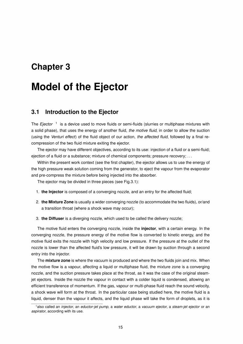
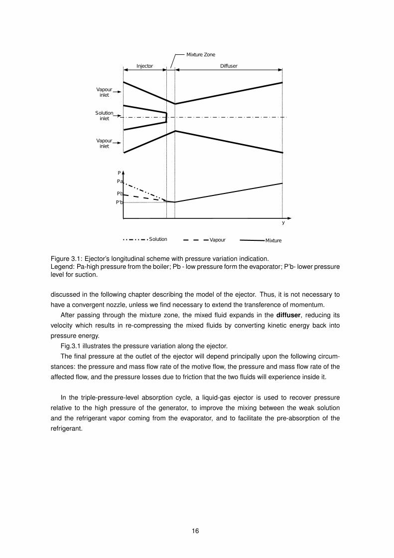
The ejector may be divided in three pieces (see Fig.3.1):
1. the Injector is composed of a converging nozzle, and an entry for the affected fluid;
2. the Mixture Zone is usually a wider converging nozzle (to accommodate the two fluids), or/and
a transition throat (where a shock wave may occur);
3. the Diffuser is a diverging nozzle, which used to be called the delivery nozzle;
The motive fluid enters the converging nozzle, inside the injector, with a certain energy. In the
converging nozzle, the pressure energy of the motive flow is converted to kinetic energy, and the
motive fluid exits the nozzle with high velocity and low pressure. If the pressure at the outlet of the
nozzle is lower than the affected fluid’s low pressure, it will be drawn by suction through a second
entry into the injector.
The mixture zone is where the vacuum is produced and where the two fluids join and mix. When
the motive flow is a vapour, affecting a liquid or multiphase fluid, the mixture zone is a converging
nozzle, and the suction pressure takes place at the throat, as it was the case of the original steam-
jet ejectors. Inside the nozzle the vapour in contact with a colder liquid is condensed, allowing an
efficient transference of momentum. If the gas, vapour or multi-phase fluid reach the sound velocity,
a shock wave will form at the throat. In the particular case being studied here, the motive fluid is a
liquid, denser than the vapour it affects, and the liquid phase will take the form of droplets, as it is
1also called an injector, an eductor-jet pump, a water eductor, a vacuum ejector, a steam-jet ejector or anaspirator, according with its use.
15
y
P
Solution Vapour Mixture
Pa
Pb
P'b
Vapourinlet
Vapourinlet
Solutioninlet
Injector Diffuser
Mixture Zone
Figure 3.1: Ejector’s longitudinal scheme with pressure variation indication.Legend: Pa-high pressure from the boiler; Pb - low pressure form the evaporator; P’b- lower pressurelevel for suction.
discussed in the following chapter describing the model of the ejector. Thus, it is not necessary to
have a convergent nozzle, unless we find necessary to extend the transference of momentum.
After passing through the mixture zone, the mixed fluid expands in the diffuser, reducing its
velocity which results in re-compressing the mixed fluids by converting kinetic energy back into
pressure energy.
Fig.3.1 illustrates the pressure variation along the ejector.
The final pressure at the outlet of the ejector will depend principally upon the following circum-
stances: the pressure and mass flow rate of the motive flow, the pressure and mass flow rate of the
affected flow, and the pressure losses due to friction that the two fluids will experience inside it.
In the triple-pressure-level absorption cycle, a liquid-gas ejector is used to recover pressure
relative to the high pressure of the generator, to improve the mixing between the weak solution
and the refrigerant vapor coming from the evaporator, and to facilitate the pre-absorption of the
refrigerant.
16
3.2 Injector
Nomenclature
A Cross Section Area of the Nozzle [m2]
CV Control Volume [m3]
CS Control Surface [m2]
D Diameter of the Nozzle [m]
e Specific energy [J/kg]
e Specific internal energy [J/kg]
f Darcy friction factor
F Total Force vector [N ]
f Specific force vector [N/kg]
h Specific entalphy [J/kg]
L Total length of the nozzle [m]
M Mass flow rate [kg/s]
m Unit vector parallel to the surface
n Unit normal vector on the outside of the surface
p Pressure [Pa]
pi Pressure at the lateral surface [Pa]
Q, Q Heat and rate of heat added to the system [J ], [W ]
S, S Surface, normal surface vector (nS) [m2]
t Time [s]
T Temperature [K]
u Cross section’s mean velocity [m/s]
u Velocity vector [m/s]
V Volume [m3]
v Specific volume [m3/kg]
x Ammonia’s mass fraction [kg/kg]
W Rate of work delivered to the system [W ]
17
Greek Letters
α angle between the axis of the nozzle and the line segment that connects both the inlet and the
outlet cross section boundary circumference.
φ kinetic energy correction factor
ν momentum correction factor
ρ Density [kg/m3]
τ Shear stress [N/m2]
Subscripts
• 1-inlet (also in)
• 2-outlet (also out)
Position coordinates (cylindrical, orthogonal: r, β, y):
y length coordinate, parallel to the axis of the nozzle and along the flow direction.
r radial coordinate.
β angle coordinate.
z absolute high.
18
3.2.1 Model
Description and Assumptions
1 2
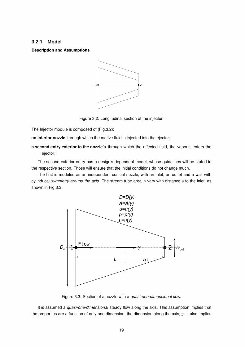
Figure 3.2: Longitudinal section of the injector.
The Injector module is composed of (Fig.3.2):
an interior nozzle through which the motive fluid is injected into the ejector;
a second entry exterior to the nozzle’s through which the affected fluid, the vapour, enters the
ejector;
The second exterior entry has a design’s dependent model, whose guidelines will be stated in
the respective section. Those will ensure that the initial conditions do not change much.
The first is modeled as an independent conical nozzle, with an inlet, an outlet and a wall with
cylindrical symmetry around the axis. The stream tube area A vary with distance y to the inlet, as
shown in Fig.3.3.
1 2Flow
y
u=u(y)p=p(y)
A=A(y)
���(y)
D=D(y)
D
L �
Din out
Figure 3.3: Section of a nozzle with a quasi-one-dimensional flow.
It is assumed a quasi-one-dimensional steady flow along the axis. This assumption implies that
the properties are a function of only one dimension, the dimension along the axis, y. It also implies
19
that area change along the nozzle is a main cause for the flow properties’ variation. At the same
time, It is assumed that the properties are uniform across any given cross section of the flow, where
A = A(y), p = p(y), ρ = ρ(y) and u = u(y), and that they represent values that are some kind of
mean of the actual flow properties distributed over the cross section.
A point worthy of attention is the velocity near the wall. The model assumes a uniform velocity
across the cross section, and hence, it may seem that the no slip condition do not hold. However,
the model is assumed quasi-one-dimensional, and the uniform velocity represent some kind of mean
of the actual flow profile. To take into account the velocity profile along the cross section, correction
factors will be multiplied to the results of integration including the velocity. Further, the actual physical
flow velocity near the wall may be slightly different from zero, and friction losses will be taken into
account with a correlation based on experimental results that use the mean velocity value in the
calculation.
The actual physical flow through the variable-area duct is four-dimensional, and the flow proper-
ties vary as a function of the three spacial coordinates and time. Nevertheless, it is assumed that
the flow is completely developed, a state in which its properties suffer only minor variations with
time. Moreover, the wall cylindrical symmetry around the axis, plus the fact that the fluid flow along
the axis, foresee that the macro behaviour of the fluid will be perceived as varying only along the
dimension y.
In the following sections the governing equations will be derived for this case as exact repre-
sentations of the conservation equations, although applied to a physical model that is approximate.
Hence, the overall physical integrity of the flow is not compromised. For the problem subject of this
thesis (see the introduction in chapter 1), the quasi-one-dimensional results are sufficient.
Assumptions
Several other assumptions were made to characterize the injector’s flow. Synthesizing, it is assumed
a flow which is:
1. ∂/∂t = 0, steady (completely developed, variations with time are negligible).
2. Q = 0, adiabatic (there is no energy transferred through the walls).
3. ∂/∂r ∼ 0 and ∂/∂β ∼ 0, one-dimensional (symmetry around the axis, properties vary only
with y).
4. with a negligible gravity influence (not worth considering / dimensionally insignificant for the
problem).
Geometry
The cross-section area at some distance y from the inlet is given by
A(y) =π
4D(y)2 (3.1)
The diameter at some distance y from the inlet, which have a diameter Din, is given by:
D(y) = Din − 2y tanα (3.2)
where α is the nozzle’s characteristic angle.
20
Integrating Eq.(3.2) along the axis leads to
∆D = −2L tanα (3.3)
where ∆D = Dout −Din is the difference between the outlet and the inlet diameters of the nozzle,
and L is the total nozzle’s length. For a given inlet diameter, Eq.(3.3) shows that one needs only two
parameters from the three remaining, Dout, L, α, to define the geometry of a nozzle.
Differentiating D(y), Eq.(3.2), yields
dD
dy= −2 tanα (3.4)
Thus, differentiating A(y), yields
dA
dy=
d
dD
(π4D2) dDdy
=π
2DdD
dy= −πD tanα (3.5)
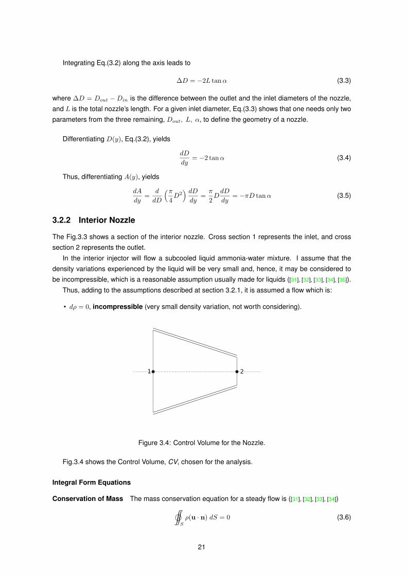
3.2.2 Interior Nozzle
The Fig.3.3 shows a section of the interior nozzle. Cross section 1 represents the inlet, and cross
section 2 represents the outlet.
In the interior injector will flow a subcooled liquid ammonia-water mixture. I assume that the
density variations experienced by the liquid will be very small and, hence, it may be considered to
be incompressible, which is a reasonable assumption usually made for liquids ([31], [32], [33], [34], [35]).
Thus, adding to the assumptions described at section 3.2.1, it is assumed a flow which is:
• dρ = 0, incompressible (very small density variation, not worth considering).
1 2
Figure 3.4: Control Volume for the Nozzle.
Fig.3.4 shows the Control Volume, CV, chosen for the analysis.
Integral Form Equations
Conservation of Mass The mass conservation equation for a steady flow is ([31], [32], [33], [34])
©∫∫S
ρ(u · n) dS = 0 (3.6)
21
When integrated over the control volume in Fig.3.4, leads to
M1 = M2 ⇔ u1A1 = u2A2 (3.7)
or u2 =Mρ1A2
=M v1A2
(3.8)
The ammonia’s mass is also conserved,
©∫∫
xρ(u · n) dS = 0 (3.9)
and its conservation equation integrated leads to
x1 = x2 (3.10)
Conservation of Momentum The momentum conservation equation for a steady flow is ([31], [32],
[33])
F =©∫∫
u ρ(u · n) dS (3.11)
The total force on the control volume is given by [33]:
F =©∫∫∫
V
ρ f dV −©∫∫
p dS +©∫∫
τ m dS (3.12)
where dS = ndS for convenience.
Assuming no body forces acting on the fluid inside the control volume (the gravity force is ne-
glected), the total force is composed of the forces acting on the boundary of the control volume, the
control surface. These are the sum of the pressure force and shear stress, and Eq.(3.12) becomes
F = −©∫∫
p dS +©∫∫
τ m dS (3.13)
Let us take the positive y direction as that acting toward the right, along the flow. Dividing the
control surface in inlet, outlet, and lateral, and integrating the pressure term in Eq.(3.13) on the
control surface in Fig.3.4, leads to[−©∫∫
p dS]y
= p1A1 − p2A2 +[−∫∫
lateral surfacepi dS
]y
(3.14)[−©∫∫
p dS]r
= 0 (3.15)[−©∫∫
p dS]β
= 0 (3.16)
Integrating the friction term on the control surface, we get
©∫∫
τ m dS =∫∫
lateral surfaceτ m dS (3.17)
As noticed for the pressure, the friction force components along the radius and angle cancel out
due to the symmetry of the flow model.
Substituting Eqs.(3.14) to (3.17) in Eq.(3.13), and substituting this in Eq.(3.11), and integrating
the moment flow terms over the control volume in Fig.3.4, leads to
p1A1 − p2A2 +[−∫∫
lateral surfacepi dS
]y
+[∫∫
lateral surfaceτ m dS
]y
= ρν2u22A2 − ρν1u2
1A1 (3.18)
22
where ν1 and ν2 are the momentum correction factors that take into account the flow profile as
mentioned before 2 . As the flow will probably be fully turbulent, we may approximate both correction
factors to 1, ν ≈ 1 [31], [32].
Reorganizing the equation, we get[−∫∫
lateral surfacepi dS
]y
= m1(u2 − u1) + p2A2 − p1A1 −[∫∫
lateral surfaceτ m dS
]y
(3.19)
This lateral pressure applied by the lateral surface on the fluid, can be shown to be the reaction to
the pressure exerted by the fluid on the surface, which may result in a non-zero force applied on the
surface (as shown in annex A.2), and kept in equilibrium at the flange which maintains the nozzle’s
position.
Conservation of Energy The energy conservation equation for a steady flow is ([31], [32], [33])
Q+ W =©∫∫S
e ρ(u · n)dS (3.20)
Reminding the assumptions made at the beginning of the chapter, in section 3.2.1, it is an adia-
batic flow, with negligible gravity effect (insignificant δz). Hence, Q = 0, and e = e+ u2/2, where e is
the specific internal energy.
The rate of work done on the fluid due to pressure and friction forces, wich were discussed in the
last section and are described in Eq.(3.13), is found by the relation for the rate of work on a moving
body, W = F · u, leading to:
W = −©∫∫
p u · dS +©∫∫
τ u ·mdS (3.21)
Considering the assumptions mentioned, and including the work due to pressure forces in the
energy integral, Eq.(3.20) may be rewriten as
©∫∫ (
h+u2
2
)ρ(u · n)dS =©
∫∫τ u ·mdS (3.22)
where h is the specific enthalpy, given by h = e+ p/ρ.
When integrated over the control volume in Fig.3.4, Eq.(3.22) leads to
M[(h2 − h1) +
12
(φ2u22 − φ1u
21)]
=∫∫
lateral surfaceτ u ·m dS (3.23)
where φ1 and φ2 are the kinetic energy correction factors that take into account the flow profile as
mentioned before. Both the kinetic energy correction factors, φ1 and φ2, have the value 2 for laminar
flow and ≈ 1 for turbulent flow [31], [32]. As we shall see later, the flow will be turbulent inside the
nozzle and we may thus ignore the correction factor.
We may divide the friction work integral in Eq.(3.23) in two components:
M[(h2 − h1) +
12
(φ2u22 − φ1u
21)]
=(∫∫
lateral surfaceτ u ·m dS
)y
+(∫∫
lateral surfaceτ u ·m dS
)r,β
(3.24)
where the two sets of coordinate indexed curved brackets stand for the component of the integral
related to the friction force along the flow and the component of the integral related to the friction
force perpendicular to the flow direction, respectively, noting that the velocity along the section is not
2See section 3.2.1 about the nozzle’s model.
23
always parallel to the flow direction but to the unit vector tangent to the surface, in spite of the fact
that the quasi-unidimensional uniform velocity considered in the model is. Moreover, although the
symmetrical friction force components perpendicular to the y axis cancel out, the dot product of it
and the symmetrical velocity along the perimeter do not. Therefore, the first component of the work
due to friction forces is related with the friction force component along the flow, responsible by the
pressure loss, and the second component is related to the section contraction of the nozzle.
The irreversible mechanical loss term vary along the nozzle. Smaller areas will imply a faster flux,
which imply a greater friction. Therefore, the energy loss depends on the velocity, whose variation
will depend on the energy loss. Hence, this term is not of trivial numerical integration.
24
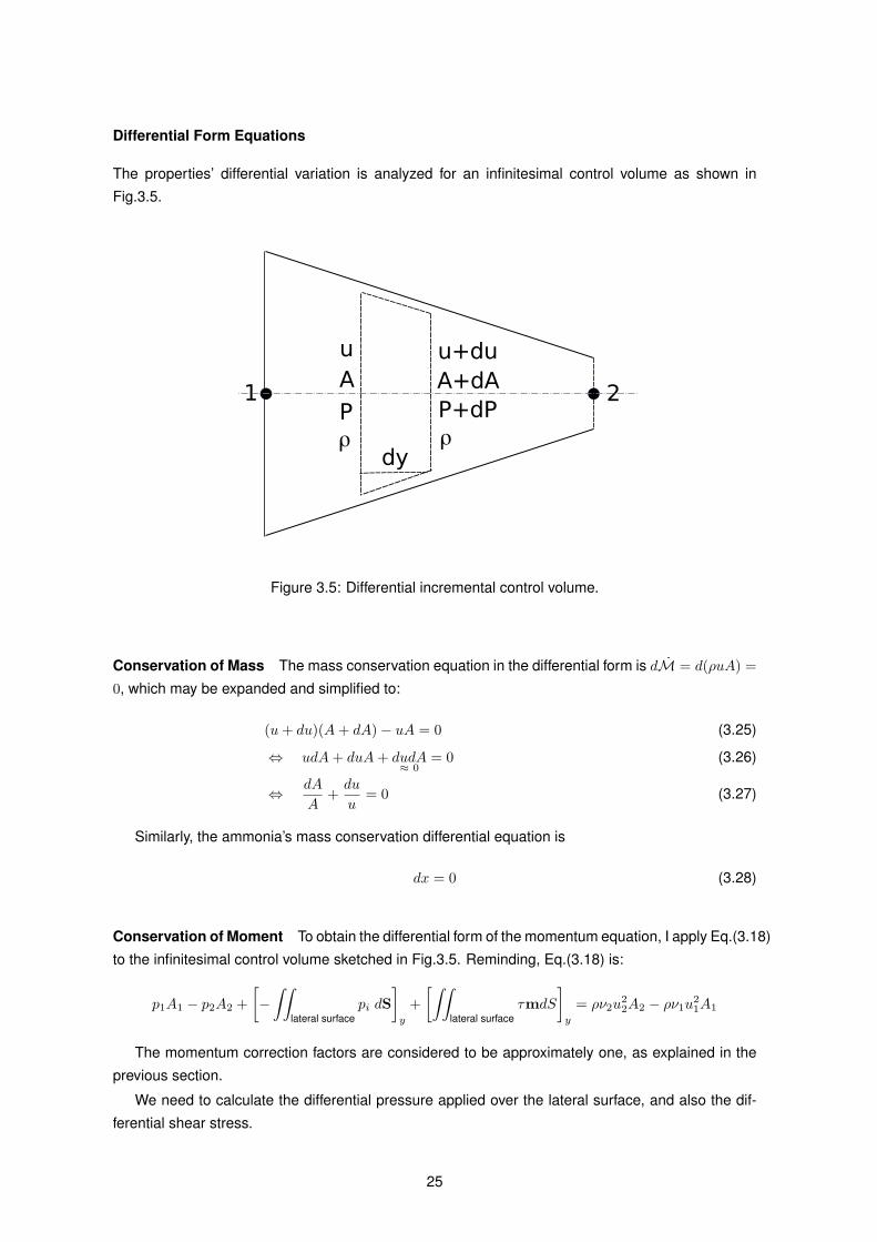
Differential Form Equations
The properties’ differential variation is analyzed for an infinitesimal control volume as shown in
Fig.3.5.
1 2A A+dA
dy
P P+dP
u u+du
� �
Figure 3.5: Differential incremental control volume.
Conservation of Mass The mass conservation equation in the differential form is dM = d(ρuA) =
0, which may be expanded and simplified to:
(u+ du)(A+ dA)− uA = 0 (3.25)
⇔ udA+ duA+ dudA≈ 0
= 0 (3.26)
⇔ dA
A+du
u= 0 (3.27)
Similarly, the ammonia’s mass conservation differential equation is
dx = 0 (3.28)
Conservation of Moment To obtain the differential form of the momentum equation, I apply Eq.(3.18)
to the infinitesimal control volume sketched in Fig.3.5. Reminding, Eq.(3.18) is:
p1A1 − p2A2 +[−∫∫
lateral surfacepi dS
]y
+[∫∫
lateral surfaceτmdS
]y
= ρν2u22A2 − ρν1u2
1A1
The momentum correction factors are considered to be approximately one, as explained in the
previous section.
We need to calculate the differential pressure applied over the lateral surface, and also the dif-
ferential shear stress.
25
We have the following pressure relation (see annex A.1) :[∫∫lateral surface
pi dS]
y= sinα
∣∣∣∣∫∫lateral surface
pi dS∣∣∣∣ (3.29)∣∣∣∣∫∫
lateral surfacepi dS
∣∣∣∣ ≈ limdS→0
∑i
pi dS = limdy→0
∑i
pi(y)dS
dydy (3.30)
The pressure vary along the infinitesimal lateral surface, between p at the differential inlet and
p + dp at the differential outlet. As we are talking about infinitesimal variations, we may consider
the lateral pressure constant. There are several options for its value: equal to the differential inlet
pressure, pi = p; the linear mean value pi = p + dp2 ; or another kind of mean. It is usual to choose
the first option in the literature ([31], [32], [33]), which seems to be the natural and more convenient
choice, as the lateral pressure is the wall reaction to the fluid pressure exerted on it, and the fluid
enters the infinitesimal control volume with the pressure p.
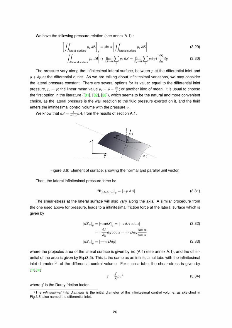
We know that dS = 1sinαdA, from the results of section A.1.
nm
�y
r
Figure 3.6: Element of surface, showing the normal and parallel unit vector.
Then, the lateral infinitesimal pressure force is:
|dFp,lateral|y = |−p dA| (3.31)
The shear-stress at the lateral surface will also vary along the axis. A similar procedure from
the one used above for pressure, leads to a infinitesimal friction force at the lateral surface which is
given by
|dFτ |y = |τmdS|y = |−τdA cotα| (3.32)
= τdA
dydy cotα = τπDdy
tanαtanα
|dFτ |y = |−τπDdy| (3.33)
where the projected area of the lateral surface is given by Eq.(A.4) (see annex A.1), and the differ-
ential of the area is given by Eq.(3.5). This is the same as an infinitesimal tube with the infinitesimal
inlet diameter 3 of the differential control volume. For such a tube, the shear-stress is given by
[31],[32]
τ =f
8ρu2 (3.34)
where f is the Darcy friction factor.
3The infinitesimal inlet diameter is the initial diameter of the infinitesimal control volume, as sketched inFig.3.5, also named the differential inlet.
26
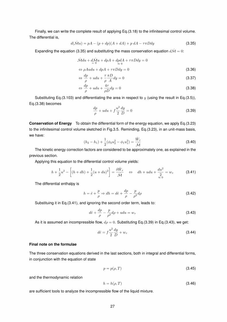
Finally, we can write the complete result of applying Eq.(3.18) to the infinitesimal control volume.
The differential is,
d(Mu) = pA− (p+ dp)(A+ dA) + p dA− τπDdy (3.35)
Expanding the equation (3.35) and substituting the mass conservation equation dM = 0:
Mdu+ dM= 0
u+ dpA+ dpdA≈ 0
+ τπDdy = 0
⇔ ρAudu+ dpA+ τπDdy = 0 (3.36)
⇔ dp
ρ+ udu+
τ
ρ
πD
Ady = 0 (3.37)
⇔ dp
ρ+ udu+
4τρD
dy = 0 (3.38)
Substituting Eq.(3.103) and differentiating the area in respect to y (using the result in Eq.(3.5)),
Eq.(3.38) becomesdp
ρ+ udu+ f
u2
2dy
D= 0 (3.39)
Conservation of Energy To obtain the differential form of the energy equation, we apply Eq.(3.23)
to the infinitesimal control volume sketched in Fig.3.5. Reminding, Eq.(3.23), in an unit-mass basis,
we have:
(h2 − h1) +12
(φ2u22 − φ1u
21) =
Wτ
M(3.40)
The kinetic energy correction factors are considered to be approximately one, as explained in the
previous section.
Applying this equation to the differential control volume yields:
h+12u2 −
[(h+ dh) +
12
(u+ du)2]
=δWτ
M⇔ dh+ udu+
du2
2≈ 0
= wτ (3.41)
The differential enthalpy is
h = e+p
ρ⇒ dh = de+
dp
ρ− p
ρ2dρ (3.42)
Substituing it in Eq.(3.41), and ignoring the second order term, leads to:
de+dp
ρ− p
ρ2dρ+ udu = wτ (3.43)
As it is assumed an incompressible flow, dρ = 0. Substituting Eq.(3.39) in Eq.(3.43), we get:
de = fu2
2dy
D+ wτ (3.44)
Final note on the formulae
The three conservation equations derived in the last sections, both in integral and differential forms,
in conjunction with the equation of state
p = p(ρ, T ) (3.45)
and the thermodynamic relation
h = h(ρ, T ) (3.46)
are sufficient tools to analyze the incompressible flow of the liquid mixture.
27
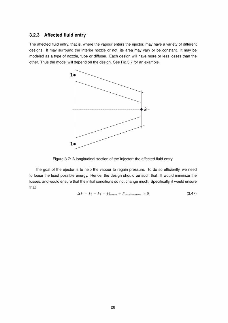
3.2.3 Affected fluid entry
The affected fluid entry, that is, where the vapour enters the ejector, may have a variety of different
designs. It may surround the interior nozzle or not, its area may vary or be constant. It may be
modeled as a type of nozzle, tube or diffuser. Each design will have more or less losses than the
other. Thus the model will depend on the design. See Fig.3.7 for an example.
1
2
1
Figure 3.7: A longitudinal section of the Injector: the affected fluid entry.
The goal of the ejector is to help the vapour to regain pressure. To do so efficiently, we need
to loose the least possible energy. Hence, the design should be such that: It would minimize the
losses, and would ensure that the initial conditions do not change much. Specifically, it would ensure
that
∆P = P2 − P1 = Plosses + Pacceleration ≈ 0 (3.47)
28
3.3 Diffuser
Nomenclature
Indexes
N phase index: C-Continuous Phase (vapour); D-Disperse Phase (liquid);
i coordinate system component of a vector
in inlet of the diffuser
Parameters and Variables
A Cross Section Area of the Diffuser [m2]
AN Equivalent cross section area for an individual phase [m2]
CV Control Volume [m3]
CS Control Surface [m2]
D Diameter [m]
e Specific energy [J/kg]
e Specific internal energy [J/kg]
E Total energy [J ]
f Darcy friction factor
F General force vector [N ]
F Force vector component along the flow (axis y) [N ]
g gravitational acceleration [m/s2]
h Specific entalphy [J/kg]
j Superficial velocity [m/s]
m Mass flux [kg/(m2s)]
M Mass flow rate [kg/s]
M→N Mass flow rate transferred to phase N . [kg/s]
M Moment flow rate [N/m]
M→N Moment flow rate transferred to phase N . [N/m]
m Unit vector parallel to the surface
n Unit vector normal to the surface
n number of droplets per element of volume. [m−3]
29
p Pressure [Pa]
Q, Q Heat and rate of heat added to the system. [J ], [W ]
Q→N Rate of heat transferred to phase N . [W ]
S Surface of the diffuser [m2]
t Time [s]
uN Mean velocity of phase N . [m/s]
u Velocity vector [m/s]
vD Volume of a droplet [m3]
x Ammonia’s mass fraction [kg/kg]
W , W Work and rate of work delivered to the system [J ], [W ]
α angle between the flow direction (the axis direction) and the line that connects both the inlet
cross section boundary circumference and the outlet cross section boundary circumference.
ε Mean phase content. [m3/m3]
Φ Fraction of ammonia transferred with the total mass transfer. [(kg/s)/(kg/s)]
ρ Density. [kg/m3]
θ angle between the gravitational acceleration and the flow direction.
τ Shear stress. [N/m2]
ξN Weight of the mass transferred over the N th phase total flow rate.
Position coordinates (cylindrical, orthogonal: r, β, y):
y length coordinate, parallel with the axis of the diffuser and along the flow direction.
r radial coordinate.
β angle coordinate.
z absolute high.
30
3.3.1 Multiphase Flow Notation and basic Definitions and Relations
The notation that will be used is close to the standard used in the bibliography referred (in particular
[35], [34], [31], [33], [36]). However, as the subject of this thesis deal with different fields of science that
focus on certain aspects of the phenomena over others , some of the standard notation of one field
will conflict with the notation of another field. For example, the cartesian coordinate x of one, is the
ammonia’s liquid mass fraction x of the other. Hence, the notation has been slightly modified in order
to get around those situations, while retaining an easy association with the phenomenon described
by the variables and minimizing possible confusion with other notations.
The subscripts that can be attached to a property will consist of a group of uppercase subscripts
followed by lowercase subscripts. The lower case subscript i is used in the conventional manner to
denote vector components. A single uppercase subscript N will refer to the property of a specific
phase or component. The uppercase subscript B will be the generic reference to the property of
a phase or component in sums. However, letters such as N = C (continuous phase) and N = D
(disperse phase) will be used for clarity. Finally two uppercase subscripts will imply the difference
between the two properties for the two single uppercase subscripts.
The mean-phase content of a component or phase, εN , is defined as the time-averaged volume
fraction of that component in the mixture or as the time-averaged area fraction in a given cross
section (The two definitions are taken to be equivalent for the purposes of the present chapter).
εN =VN∑B VB
=AN∑B AB
(3.48)
The volume flow rate fraction, εNi, is given by
εNi =VNi∑B VBi
(3.49)
where VNi and VBi are the volume flow rates for the Nth and Bth components in the ith direction,
respectively.
31
The superficial velocities or volumetric fluxes 4 for each component will be denoted by jNi
(i = 1, 2 or 3 in three dimensional flow) and the total volumetric flux is given by
ji =∑N
jNi (3.50)
The mass fluxes are denoted by mNi, and the densities for individual components by ρN . It
follows that
mNi = ρN jNi mi =∑N
ρN jNi (3.51)
The average velocities for specific phases are denoted by uNi, and the relative velocity between
phase D and C is
uDCi = uDi − uCi (3.52)
The volumetric flux of a component and its velocity are related by
jNi = εNuNi and thus ji =∑N
εNuNi (3.53)
The multiphase mixture has certain mixture properties of which the most readily evaluated is the
mixture density denoted by
ρ =∑N
ρN εN (3.54)
The mixture specific enthalpy, h, and mixture specific entropy, s, being defined as per unit mass
rather than per unit volume are weighted according to
ρh =∑N
ρN εNhN ; ρs =∑N
ρN εNsN (3.55)
Other properties such as the mixture viscosity or thermal conductivity cannot be reliably obtained
from such simple weighted means.
One-dimensional flow
The following fractional properties are only relevant in the context of one-dimensional flows.[35]
The mass fraction of a phase or component is simply given by
XN =ρN εNρ
(3.56)
The mass quality, or simply the quality, QN , is the ratio of the mass flux of phase N , to the total
mass flux,
QN =mN
m=
ρN jN∑B ρBjB
(3.57)
For a tube with a constant cross-section area, the volume flux of a component is defined as
jN =˙VNA
(3.58)
where A is the channel cross-sectional area.
And the average component velocity is
uN =˙VN
εNA(3.59)
4volume flow rate per unit area
32
Two phases flow
When only two components or phases are present it is often redundant to use subscripts on the
volume fraction and the qualities since:
εC = 1− εD (3.60)
XC = 1−XD (3.61)
QC = 1−QD (3.62)
Chemical Notation
Each component of the mixture of phases is composed of a chemical mixture of ammonia and water.
A single uppercase subscript N ′ will refer to a particular chemical component (NH3, H2O).
The mass density for each component of the chemical mixture, ρN ′ [kg m−3], and the molar
concentration, CN ′ [kmol m−3], are related by the molar mass, MN ′ [kg m−3] as
ρN ′ = MN ′CN ′ (3.63)
The chemical mixture density, and thus, the density of each phase, is given by
ρN =∑B′
ρN,B′ with B′ = NH3, H2O (3.64)
The ammonia’s mass fraction of a specific phase is given by
xN =ρN,NH3
ρN(3.65)
As this is a binary mixture, the water’s mass fraction is obviously xN,H2O = 1− xN .
The molar fraction is
xN,N ′ =CN,N ′
CNand
∑B′
xN,B′ = 1 (3.66)
The partial pressures are given by
pN,N ′ = xN,N ′ pN (3.67)
The chemical mixture properties definitions and relations, used for each phase component of the
mixture, are those mentioned in [37]. In particular, the chemical mixture’s viscosity use the relation
developed in [38].
33

34
3.3.2 Model
The injector will introduce two fluids into the diffuser, where they will be mixed. The motive fluid will
be in the liquid phase. However, given certain conditions at the nozzle’s inlet, the pressure at the
nozzle’s exit may be small enough to start evaporation. Nevertheless, the quantities involved would
be so small that are not worthy of taking into account as we shall see later in the results section for
the nozzle.
The affected fluid will be composed of two phases, liquid and gaseous. The multiphase flow
is a very diluted vapour. It is sufficient to solve it for the velocity, pressure and temperature of the
continuous suspending fluid while ignoring the sparse liquid droplets.
It is then assumed that the multiphase flow in the diffuser will be a mixture of two distinct compo-
nents, representing each, two different phases of the chemical mixture consisting of ammonia and
water, which are not in equilibrium. It is assumed that the liquid phase is completely composed of
the motive fluid, and that the vapour phase is composed of the affected fluid.
To advance further in the development of a model, it is necessary to infer which type of two-
phase flow regime will thrive inside the diffuser. The flow regime inside the diffuser should be
dispersive, consisting of a disperse phase in the form of finite drops distributed in a connected
volume of continuous phase. Such an approach was followed by Jelinek [39] and Ana [7]. Any clear
formula was not found to infer the flow regime at the nozzle’s outlet. However, some intuitive formulae
are described in [35], and this type of regime is prevalent in observations at similar conditions. One
can infer the high probability that such a regime will exist inside the diffuser: The fluid mixture
reaches the nozzle’s outlet with high velocity due to the acceleration subjected to inside. There, the
high velocity fluid, experiencing an oscillation of the velocity (characteristic of the turbulent regime),
encounters the exit’s wall finnish, and then exits to the outside mixture zone, where it will flow as
a free stream, and where it will meet the vapour. When the motive fluid in the liquid state exits
the nozzle, the friction forces at the wall finnish have the effect of disaggregating the fluid (also
connected to the coanda effect [40]). The free flowing mixture will tend to break up, and the surface
forces will reorganize the fluid in the most stable configuration: almost spherical drops.
Therefore, the approach followed is a two-fluid model : one disperse phase consisting of liquid
droplets, and one continuous phase consisting of vapour.
The disperse phase is treated as a second continuous phase intermingled and interacting with
the continuous phase, for the purpose of the conservation equations, and is treated as discrete
near spherical droplets for the purpose of the interaction between phases. The analyses are im-
plicitly confined to those circumstances in which the interactions between neighboring droplets are
negligible, and they will reveal that both treatments of the disperse phase are equivalent.
It is further assumed a quasi-one-dimensional flow along the diffuser’s axis, using averaged
quantities over the cross section, as it was done for the injector in section 3.2.1.
The model assumes an infinitesimal control volume as shown in Fig.3.8. The infinitesimal volume
must be such that its length is much smaller than the typical distance over which the flow properties
vary significantly, so that it is possible to define derivatives of the flow properties within the flow field.
It must also be very much larger than the size of the individual phase elements (the droplets), a
condition necessary in order that each averaging volume contain representative samples of each of
the phases (see Fig.3.9).
35
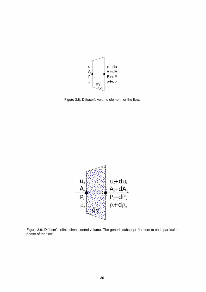
A A+dA
dy
P P+dP
u u+du
� ��+d
�
Figure 3.8: Diffuser’s volume element for the flow.
A A+dA
dy
P P+dP
u u+du
� ��+d
NN
N
N
N
N
NN
N N
NN
Figure 3.9: Diffuser’s infinitesimal control volume. The generic subscript N refers to each particularphase of the flow.
36
In the sections that follow, we proceed to develop the effective differential equations of motion for
the diffuser flow assuming that these conditions hold.
Assumptions
Several other assumptions were made to characterize the Diffuser’s flow.
Synthesizing, it is assumed a flow which . . .
1. ∂/∂t = 0, is steady (completely developed, variations with time are negligible).
2. Q = 0, is adiabatic (there is no energy transfered through the walls).
3. ∂/∂r ∼ 0 and ∂/∂β ∼ 0, is one-dimensional (symmetry around the axis, properties vary only
with y).
4. has a negligible gravity influence (not worth considering / dimensionally insignificant; do not
affect the flow of the droplets, within the dimensions in the study; very small ∆z).
5. is in a multiphase state: composed of a disperse liquid phase in the form of droplets and a
surrounding continuous vapour phase.
6. dρD = 0, has an incompressible liquid phase (very small density variation for the liquid
phase, not worth considering) (as considered in section 3.2.2)
7. is composed of droplets with the same size (an average droplet diameter is considered, it
is assumed that the gradient of the droplets size contribution to the fluid macro-dynamics is
negligible).
8. has negligible interactions between droplets.
9. has a high enough number of droplets per infinitesimal control volume in order that each
averaging volume contain representative samples of each of the phases.
37
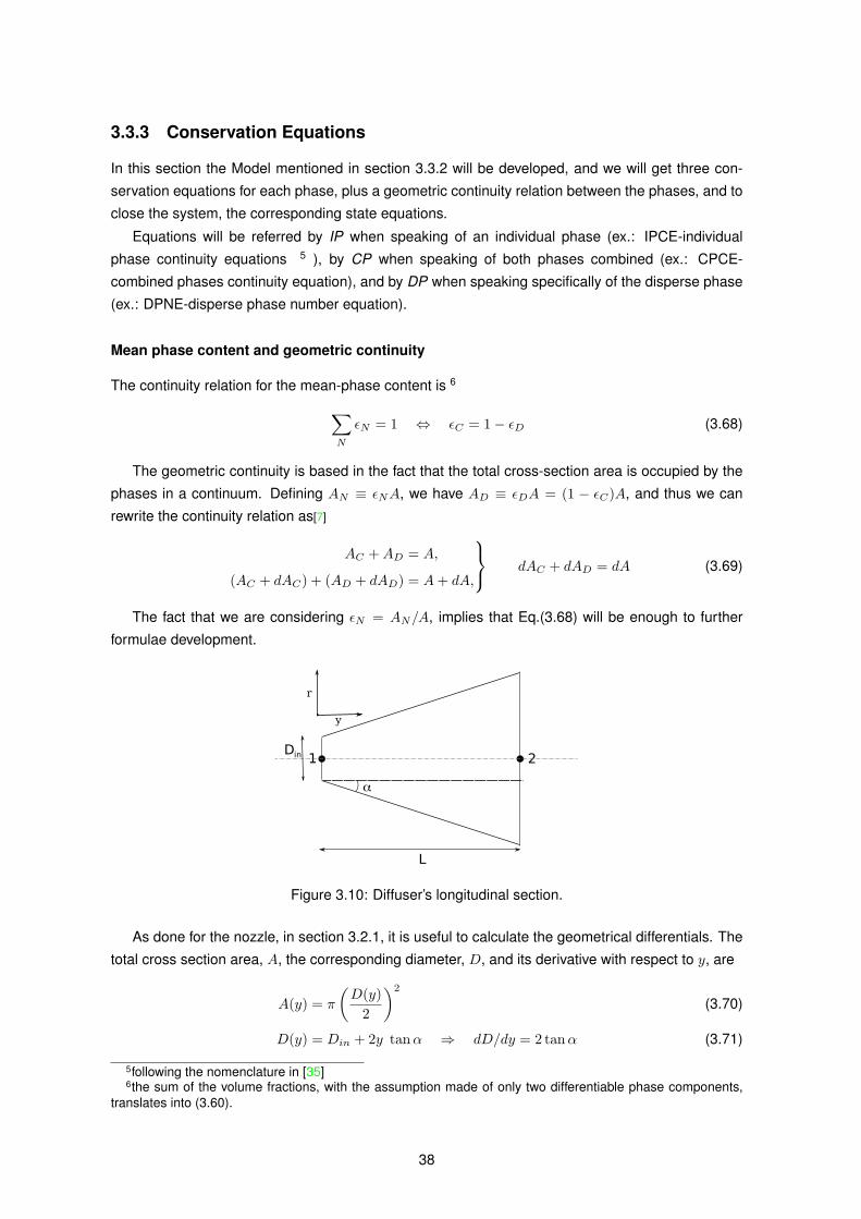
3.3.3 Conservation Equations
In this section the Model mentioned in section 3.3.2 will be developed, and we will get three con-
servation equations for each phase, plus a geometric continuity relation between the phases, and to
close the system, the corresponding state equations.
Equations will be referred by IP when speaking of an individual phase (ex.: IPCE-individual
phase continuity equations 5 ), by CP when speaking of both phases combined (ex.: CPCE-
combined phases continuity equation), and by DP when speaking specifically of the disperse phase
(ex.: DPNE-disperse phase number equation).
Mean phase content and geometric continuity
The continuity relation for the mean-phase content is 6
∑N
εN = 1 ⇔ εC = 1− εD (3.68)
The geometric continuity is based in the fact that the total cross-section area is occupied by the
phases in a continuum. Defining AN ≡ εNA, we have AD ≡ εDA = (1 − εC)A, and thus we can
rewrite the continuity relation as[7]
AC +AD = A,
(AC + dAC) + (AD + dAD) = A+ dA,
dAC + dAD = dA (3.69)
The fact that we are considering εN = AN/A, implies that Eq.(3.68) will be enough to further
formulae development.
1 2
�
L
Din
y
r
Figure 3.10: Diffuser’s longitudinal section.
As done for the nozzle, in section 3.2.1, it is useful to calculate the geometrical differentials. The
total cross section area, A, the corresponding diameter, D, and its derivative with respect to y, are
A(y) = π
(D(y)
2
)2
(3.70)
D(y) = Din + 2y tanα ⇒ dD/dy = 2 tanα (3.71)
5following the nomenclature in [35]6the sum of the volume fractions, with the assumption made of only two differentiable phase components,
translates into (3.60).
38
where Din is the inlet diameter, and α in this chapter regards the diffuser’s characteristic angle (see
Fig.3.10).
Differentiating (3.70) with respect to y, we have
dA
dy=
d
dD
(π4D2) dDdy
=π
2DdD
dy= πD tanα (3.72)
Dividing Eq.(3.69) by the infinitesimal distance dy, we get Eq.(3.69) with rates of variation of the
area along the lenght y. Substituting (3.72), leads to[7]
dACdy
+dADdy− πD tanα = 0 (3.73)
Mass Conservation
The total mass flow rate is constant along the diffuser:
dM = dMC + dMD = 0 (3.74)
suIPCE - steady unidimensional Individual Phase Continuity Equations Considering the mass
transfer between the phases, it can be shown (see A.4.1) that the mass conservation equations for
a unidimensional steady flow can be simplified to (Eq.(A.42))
∂MN
∂y=dM→Ndy
(3.75)
where y is measured along the diffuser, and M→N [kg s−1] is the total mass transfer rate to the
phase N from the other phases inside the infinitesimal control volume related with the infinitesimal
length dy. The sum of all the mass transfer terms is clearly∑N M→N = 0. Such mass exchange
may result from a phase change or chemical reaction, i.e.: evaporation, condensation, absorption,
etc. It is expected that the prevalent form of mass transfer is the absorption.
The mass flow rate is given by
MN = ρN jNA = ρN εNuNA [kg s−1] (3.76)
where A(y) is the cross-sectional area, and ρN , uN , εN are cross-sectionally averaged quantities.
We can expand the mass conservation equations to
∂(ρN εNuNA)∂y
=dM→Ndy
(3.77)
Eq.s(3.77) will be referred to as the steady unidimensional Individual Phase Continuity Equations,
suIPCE 7 .
suCPCE The sum of all the suIPCEs results in a steady unidimensional Combined Phase Conti-
nuity Equation, suCPCE:
∂A
∂y
∑N
ρN εNuN +A∂
∂y
(∑N
ρN εNuN
)= 0 (3.78)
Note that only with zero relative velocity uDC (Eq.(3.52)), can we reduce this equation to a Mix-
ture Continuity Equation, which is identical to that for an equivalent single phase flow of density ρ
(Eq.(3.54)). This won’t be the case inside the diffuser.7Named basing on the equation nomenclature in [35]
39
uDPNE - Disperse Phase Number Equation
Complementary to the equations of conservation of mass is the equation governing the conservation
of the number of droplets that constitute the disperse phase. If no droplets are created or destroyed
within the elemental volume and if the number of droplets of the disperse component, D, per unit
total volume is denoted by nD [# m−3], then:
∂nD∂t
+∂(nDuD)
∂y= 0 (3.79)
This will be referred to as the unidimensional Disperse Phase Number Equation, uDPNE 8 .
Denoting the volume of the droplets of the disperse component by vD, the volume fraction of the
disperse phase is
εD = nDvD (3.80)
Substituting Eq.(3.80) into Eq.(3.77), with the non-steady term, one obtains:
∂(nDρDvD)∂t
A+∂(ρDnDvDuDA)
∂y=dM→Ddy
[kg s−1m−1] (3.81)
Expanding this equation, and using Eq.(3.79), leads to the following relation:
dM→Ddy
= nD
(∂(ρDvDA)
∂t+ uD
∂(ρDvDA)∂y
)= nD
DD
DDt(ρDvDA) (3.82)
where the last term denotes the Lagrangian derivative following the disperse phase.
To get more information, lets expand the right term to take account for the area variation:
dM→Ndy
=nD
(A
[∂(ρDvD)
∂t+ uD
∂(ρDvD)∂y
]+ uDρDvD
∂A
∂y
)(3.83)
=nD
(ADD
DDt(ρDvD) + uDρDvD
∂A
∂y
)(3.84)
dM→NnDA dy
=DD
DDt(ρDvD) +
uDρDvDA
∂A
∂y[kg s−1#−1] (3.85)
And we find that the rate of transfer of mass to the component D in each particle, ID/nD ≡dM→N
dv′ /nD [kg/s] (with dv′ = Ady), is equal to the Lagrangian rate of increase of mass, ρDvD, of
each particle, plus a term accounting for the effects related to the variation of the area.
However, the droplets are not directly affected by the diffuser area variation and we may as-
sume that the cross-section of the fluid equivalent to the total mass of droplets is constant, hence
considering null the area variation term.
The continuity equation for the disperse phase in a steady flow becomes
dM→NnD A dy
= uD∂(ρDvD)
∂y[kg s−1#−1] (3.86)
giving emphasis to the mass transfered to each droplet.
8For the general DPNE please see reference [35]
40
Ammonia’s Mass Conservation
The total ammonia mass flow rate is constant along the diffuser. Considering the mass transfer
between phases, being the total ammonia mass transfer given by Φ(xN )M→N , the ammonia mass
conservation equations are (see A.4.2 for deduction):
dxNdy
=Φ(x)− xNM(1 + ξN )
· dM→Ndy
(3.87)
with ξN ≡dM→NMN
(3.88)
where ξN is the weight of the transfered mass flow rate over the total mass flow rate. Remember
that∑N xN = 1 by definition. Φ(xN ) is a function that stands for the fraction of ammonia transferred
with the total mass transferred, defined by
Φ(xN ) =MNH3→N
M→N(3.89)
For a two-phase mixture:
dxDdy
=Φ(xC)− xDMD(1 + ξD)
· dMC→D
dy(3.90)
dxCdy
=xC − Φ(xC)MC(1− ξC)
· dMC→D
dy(3.91)
with ξD = dMC→D
MD, the weight of the mass transferred over the liquid total flow rate,
and ξC = dMC→D
MC, the weight of the mass transferred over the vapor total flow rate.
The vapour is very rich in ammonia, and its ammonia’s mass fraction is approximately one. Thus,
mostly ammonia is transferred through absorption, and we may assume Φ ≈ 1.
Linear Momentum Conservation
Newton’s second law for a steady flow says that∑F =
∫CS
u ρ (u · n)dA (3.92)
Prior to continue the development of the differential equations, let us make some modifications
to the control volume. To simplify the analysis, we deform the bounding surfaces so that they never
cut through droplets, which become everywhere within the continuous phase. As the droplets are
much smaller then the dimensions of the control volume, the required modification is correspondingly
small.
Considering the symmetry of the control volume, we need only to consider the component of
(3.92) along the length (y axis), and thus we may assume an unidimensional flow.
For density and velocity uniform over the cross section and with a source/sink term as the mo-
mentum transfer, the momentum conservation equations for steady unidimensional flow may be
written as (see appendix A.4.3, Eq.(A.57)):
1δy
(∑
F )N +M→Nδy
= MN (1 + ξN )∂uN∂y
+ uNdM→Ndy
(3.93)
where M→N is the moment flow transfered to the mixture component N .
41
Using (3.76) we may expand the above equations into
1δy
(∑
F )N +M→Nδy
= ρNuN εNA(1 + ξN )∂uN∂y
+ uNdM→Ndy
(3.94)
These are the individual phase momentum equations for a steady unidimensional flow (IPMEsu).
We will now examine the external forces acting on the component N which are independent of
the other components. For each phase, the sum of the forces acting on the control volume along the
lenght is ∑F = Fg + Fp + Fτ (3.95)
We assumed in section 3.3.2 that the gravity force is negligible, Fg � {Fp, Fτ}.
Pressure Force The total pressure force on the control surface is
Fp =©∫∫CS
p (−n) dA (3.96)
Assuming a uniform pressure over the cross sections and lateral surface, and applying Eq.(3.96) to
the differential control surface in Fig.3.9, lead us to the total pressure force given by
Fptotal = Fp + Fp+dp + Fpi
= p A− (p+ dp)(A+ dA) + pdA
= −dp A− pdA+ pdA−dp dA≈ 0
(3.97)
= −dp A (3.98)
For very small variations of pressure and area along the element of length δy, we can neglect
the second order variation term in Eq.(3.97). The lateral pressure pi was considered to be the initial
pressure p, as done for the injector (see section3.2.2), and the projection of the surface along the
flow is dA (see appendix A.1).
Then the pressure force per unit lenght is
Fpδy
= −Adpdy
(3.99)
As all the droplets are inside the control volume, the external pressure force term is applied on
the continuous component. The droplets pressure at the surface, affecting the surface tension, is
assumed in equilibrium with the continuous phase pressure. Any pressure forces dynamics between
the disperse phase and the continuous phase will be accounted in the moment interaction term.
Friction Force The total shear-stress on the control surface is
Fτ = −©∫∫CS
τ dA (3.100)
As all the droplets are inside the control volume, only the continuous phase is in contact with the
wall, and thus we can assume that only the continuous component experiences wall friction.
The procedure will be similar to that referred before for the injector in section 3.2.2. Applying
Eq.(3.100) to the differential control surface in Fig.3.9, and assuming an uniform shear stress on the
42
surface, lead us to
|δFτ |y = |τm dS|y = |τ dA cotα| (3.101)
= τdA
dydy cotα = τπDdy
tanαtanα
δFτ |y = −τπDdy (3.102)
where the projected area of the lateral surface is given by Eq.(A.4) for a diffuser (see annex A.1),
and the differential of the area is given by Eq.(3.72). This is the same as an infinitesimal tube with
the infinitesimal inlet diameter 9 of the differential control volume. For such a tube, the shear-stress
is given by [31],[32]
τ =f
8ρu2 (3.103)
where f is the Darcy friction factor.
Then the friction force per unit lenght is
δFτδy
= −f8πDρu2 (3.104)
The friction between the phases will be taken into account in the momentum interaction term.
Sum of the forces Using Eqs.(3.99) and (3.104), we can sum the forces acting on the N th phase
per unit length, without taking into account the forces between interacting components (which will be
taken into account in the second term of the left side in equation (3.94)), is
δ
δy(∑
F )N = δN (Adp
dy+f
8πDρu2) (3.105)
where δD = 0 for the disperse phase and δC = 1 for the continuous phase.
suIPME - Momentum Conservation Equations With (3.105), we can rewrite equations (3.94) as:
M→Nδy
− δN (Adp
dy+f
8πDρu2) = ρNuN εNA(1 + ξN )
∂uN∂y
+ uNdM→Ndy
(3.106)
Summing the suIPME equations, we get the Combined Phase Momentum Equation for steady
unidimensional flow, suCPME:
∂
∂y
(∑N
ρNu2N εN
)= ρg cos(θ)− dp
dy− f
2Dρu2 (3.107)
DPME - Disperse Phase Momentum Equation Let us consider the relation of the momentum
conservation equation for the disperse phase delineated in the last section with the equation of
motion for an individual drop, analogous to what we did with the DPCE (section 3.3.3).
For an individual droplet with volume vD we have that the following equation of motion:
DD
DDt(ρDvDuD) = (
∑B
FB)N→D + ρDvDg cos(θ) (3.108)
where DD/DDt is the Lagrangian time derivative following the droplet so that
DD
DDt≡ ∂
∂t+ uD
∂
∂y(3.109)
9The infinitesimal inlet diameter is the initial diameter of the infinitesimal control volume, as sketched inFig.3.9, also named the differential inlet.
43
and FB is a force exerted by the continuous phase on the droplet, which includes the force due to the
velocity and acceleration of the droplet relative to the surrounding fluid but also the buoyancy forces
due to pressure gradients within the continuous phase. The last term of Eq.(3.108) is assumed
negligible, as mentioned in the last section and in section 3.3.2.
Expanding (3.108) and using (3.85), one obtains the following form of the DPME:
ρDvDDD
DDt(uD) + uD
dM→NnDA dy
=∑B
FB (3.110)
Let us examine the implication when its steady state form is compared with the DPMEsu (Eq.(3.106)
for the disperse phase). Setting εD = nDvD, expanding and comparing the result with the equation
above, one observes that M→D = nD∑B FB . Hence, the interaction term in the disperse phase
momentum equation is simply the sum of the fluid forces acting on the individual droplets per unit
volume, as one would expect.
Energy Conservation
The law of the conservation of energy says that for a steady flow
dE
dt=dQ
dt− dW
dt=©∫∫CS
eρ(u · n)dA (3.111)
where Q denotes heat added to the system, W denotes work done by the system, and e is the
energy convected per unit mass, which is
e = h+12u2 (3.112)
where h is the specific enthalpy that take into account the work done by pressure forces and is given
by
h = e+p
ρ(3.113)
e is the internal energy per unit mass.
It can be shown (see appendix A.4.4) that the energy conservation equations for an unidimen-
sional steady flow can be simplified to
δQNδy− δWN
δy= MN (1 + ξN )
deNdy
+ eNdM→Ndy
(3.114)
This is the Individual Phase Energy Equation for a steady unidimensional flow (IPEEsu).
The IPEEsu equations may be summed into a Combined Phase Energy Equation (CPEEsu):∑N
δQNδy−∑N
δWτN
δy=∑N
ρNuN εNAdeNdy
(3.115)
It is assumed an adiabatic flow, and so there is no heat transfer in the diffuser walls. Hence, the
heat flow rate sum in Eq.(3.115) is null. However there is heat transfer between the phases that will
be addressed later in the interaction terms section.
The work of pressure and gravitational forces has already been included as impulse and potential
energy in the specific energy term Eq.(3.112).
The work flow rate in Eq.(3.114) is due to the shear-stress.
Then, the work flow rate reduces to that due to viscous stresses:
δWτ
δy=δFτδy
u = −f8πDρu3 (3.116)
44
where δFτ/δy is given by Eq.(3.104).
The disperse phase is inside the control volume, and thus the correspondent wall friction loss is
zero.
Substituting Eq.(3.116) in Eq.(3.114) lead us to
δQ→Nδy
− δN(f
8πDρu3
)= MN (1 + ξN )
deNdy
+ eNdM→Ndy
(3.117)
withdeNdy
=dhNdy
+ uduNdy
(3.118)
45

46
3.3.4 Interaction between the phases
In this chapter the interaction terms between the phases are discussed. These terms are internal to
the control volume and disappear after the sum of the individual component equations.
Nomenclature
Indexes
N phase index: C-Continuous Phase (vapour); D-Disperse Phase (liquid);
i coordinate system component of a vector
Parameters and Variables
A Constant of the classic Stokes solution.
B Constant of the classic Stokes solution.
CD Drag coefficient. [N/N ]
cpN specific heat capacity of phase N . [J kg−1K−1]
D Diameter of the droplet. [m]
D Diffusion coefficient [m2/s]
f Vortex shedding frequencies. [s−1]
FD Drag force applied on the droplet by the vapour (movement along the y axis); Moment transfer
term. [N ]
hm Coefficient for the mass transfer by convection. [kg m−2s−1]
k thermal conductivity. [J K−1m−1s−1]
M Mass flow rate absorbed by the droplet. [kg/s]
Ma Mach number.
n number of droplets per element of volume. [m−3]
Nu Nusselt number.
Pr Prandtl number
Q, Q Heat and rate of heat transferred to the droplet. [J ], [W ]
Re Reynolds number of the droplet.
S Droplet surface area.
Sc Schmidt number.
Sh Sherwood number.
Str Strouhal number.
47
T Temperature [K]
uN Mean velocity of phase N . [m/s]
uDC Relative velocity of the vapour, in relation to the droplet. [m/s]
vD Volume of a droplet [m3]
x Ammonia’s mass fraction [kg/kg]
W , W Work and rate of work delivered to the system [J ], [W ]
y length coordinate, parallel with the axis of the diffuser and along the flow direction.
µ Viscosity. [kg m−1s−1]
µS Viscosity of the surface of the sphere. [kg m−1s−1]
ν Kinetic viscosity. [m2s−1]
ρ Density. [kg/m3]
θδ Angle between the flow axis and a point on the spheric droplet surface.
ξN Weight of the mass transferred over the N th phase total flow rate.
48
Moment Transfer
The interaction between the flow components and the inertial fight for a certain position, will result
in the transfer of moment from one component to another. To understand the moment interaction
between the phases let us picture what happens to an individual droplet and then generalize it to the
other droplets.
A droplet entering the diffuser at a high velocity will be immersed in the ammonia-water vapour
mixture and will apply its superior inertia (higher mass and velocity, and lower compressibility) to
push the vapour out of its way. It does so in two ways: directly occupying the vapour’s space and
through friction at the interface, dragging the vapour along the way. Thus, it will experience both
inertial and friction forces which will cause the deceleration of the droplet and the acceleration of the
vapour.
The analysis of the potential flow of an incompressible and inviscid suspending fluid, led to a
null drag force on a body moving with constant velocity through the fluid (Jean Le Rond D’Alembert,
1752 [42]). That was a direct contradiction to measurements finding substantial drag for bodies
moving through fluids, such as air and water, especially at high velocities (High Reynolds Numbers),
called the D’Alembert’s paradox.
No satisfactory theory for the forces acting on an arbitrary body immersed in a stream flowing at
an arbitrary Reynolds number is known at present. Numerical studies and experimentation are the
usual treatment for this type of flows.
Let us consider a frame of reference moving with a droplet of arbitrary shape immersed in the
vapour flowing with the relative velocity uDC = uD − uC (Eq.(3.52)), where uD is the translation
velocity of the center of the droplet, and uC is the velocity that the vapour would have had at the
location of the droplet center in the absence of the droplet. Note that such a concept is difficult to
extend to the case of flows with interactive droplets, where the velocity that the vapour would have
had at the location of the droplet center depends on that interaction.
The fluid forces on the droplet may include forces due to buoyancy, added mass, drag, etc. For
convenience we choose one axis parallel to the vapour stream and positive upstream. The main
force on the body along this axis is called drag, and the moment about that axis, the rolling moment.
The second force perpendicular to the drag and usually bearing the weigh of the body is called the
lift, and the moment about the lift axis is called yaw. The third force component perpendicular to
both of the forces referred is called the side force, and the moment about this axis is the pitching
moment [31].
If we consider that the droplets are spherical, then we will have symmetry about any intersecting
plane. The lift, the side force, and moments disappear, and the droplet experiences only the drag
(however, some turn movement about the origin may arise due to friction asymmetry in the flow).
This type of data is commonly reported in the literature, and the sphere case is well studied [31], [32],
[33], [35], [36].
Low Reynolds Number Stokes (1851) found a solution to the drag force on a sphere in a Stokes
flow 10 [43], for very low Reynolds numbers, Re� 1.
The classical Stokes solution for flow around a sphere is derived by neglecting the convective
acceleration, whose effect is assumed to be much smaller than the effects due to viscosity. The
10The Stokes flow is the low Reynolds number limit of the Navier-Stokes equations describing the motion of aviscous liquid, where advective inertial forces are small compared with viscous forces.
49
solution to the force, FD, on the droplet in the y direction has the form [35]
FD =13πD2ρCνC
(−8uCD
D+
128AD4
+8BD2
)(3.119)
where A and B are constants to be determined from the boundary conditions on the surface of the
sphere.
Applying the Stokes boundary conditions on a solid sphere: the no-slip boundary condition (null
tangent velocity component on the sphere’s surface), in addition to the kinematic condition (null
radial velocity component on the sphere’s surface), leads to the classic Stokes solution (1851):
FD = −3πρCνCuCDD (3.120)
However, examining the magnitude of the neglected convective acceleration term, in the Navier-
Stokes equations relative to the magnitude of the retained viscous term, leads to another paradox,
the Whitehead paradox. Although the retained term will dominate close to the body (provided Re�1), there will be always a radial position beyond which the neglected term will exceed the retained
viscous term.
Oseen (1910, [44]) attempted to correct the Stokes solution by retaining in the basic equation an
approximation to the convective acceleration, that would be valid in the far field. Oseen was able to
find a closed form solution that satisfies the Stokes boundary conditions approximately:
FD = −3πρCνCuCDD(
1 +316Re
)(3.121)
Eq.(3.121) reduces to Eq.(3.120) when Re→ 0.
Proudman and Pearson (1957, [45]) and Kaplun and Lagerstrom (1957) obtained higher approx-
imations of the drag force for a flow past a sphere at low Reynolds numbers, showing that Oseen’s
solution is, in fact, the first term obtained when the method of matched asymptotic expansions is
used in an attempt to patch together consistent asymptotic solutions of the full Navier-Stokes equa-
tions for both the near field close to the sphere and the far field [35]. The next term in the expression
for the drag force:
FD = −3πρCνCuCDD(
1 +316Re+
9160
Re2 ln(Re
2
))(3.122)
The additional term leads to an error of 1% atRe = 0, 3 and therefor does not have much practical
consequence.
The most notable feature of the Oseen solution is that, contrary to the Stokes or potential flow
solutions, the geometry of the stream lines depends on the Reynolds number, and downstream of
the sphere, the streamlines are further apart and the flow is slower than in the equivalent upstream
location, an effect that increases with Reynolds number. These features of the Oseen solution are
entirely consistent with experimental observations and represent the initial development of a wake
behind the body.
Flows past spheres at Reynolds numbers from about 0, 5 to several thousand have proven in-
tractable to analytical methods, although numerical solutions are numerous. Experimentally (Taneda
1956 [46], 5 < Re < 300), it is found that a permanent vortex-ring begins to form close to the rear
stagnation point at about Re = 24. The size of the vortex-ring is nearly proportional to the logarithm
of the Reynolds number. Defining locations on the surface by the angle from the front stagnation
point, the separation point moves forward from about 130◦ at Re = 100 to about 115◦ at Re = 300.
50
In the process the wake reaches a diameter comparable to that of the sphere when Re ≈ 130 and
begins to oscillate at the rear of the permanent vortex-ring.
However, it continues to be attached to the sphere until aboutRe = 500 (Torobin and Gauvin 1959
[47]). At Reynolds numbers above about 500, vortices begin to shed and then convected downstream.
The frequency of vortex shedding has not been studied as extensively as in the case of a circular
cylinder and seems to vary more with Reynolds number. In terms of the conventional Strouhal
number, Str, defined as
Str = fD/uCD (3.123)
the vortex shedding frequencies, f , that Moller (1938) observed correspond to a range of Str varying
from 0, 3 at Re = 1000 to about 1, 8 at Re = 5000. Furthermore, as Re increases above 500 the flow
develops a fairly steady near-wake behind which vortex shedding forms an unsteady and increas-
ingly turbulent far-wake. This process continues until, at a value of Re of the order of 1000, the flow
around the sphere and in the near-wake again becomes quite steady. A recognizable boundary layer
has developed on the front of the sphere, separation settles down to a position about 84◦ from the
layer, and then the events described in the next section occur with further increase in the Reynolds
number.
Note that it was assumed negligible interaction between droplets, implying a sufficiently diluted
flow, such that a droplet is not affected by the wakes of neighboring droplets.
The Reynolds number range between 0, 5 and 1000 may exist inside the diffuser, and we must
adopt an empirical formula for the drag force in this regime. A number of empirical results are
available, for example, Klyanchko (1934) recommends
FD = −3πρCνCuCDD
(1 +
Re23
6
)(3.124)
which fits the data fairly well up to Re ≈ 1000. At Re = 1 the factor in the brackets is 1, 167 ,
whereas the same factor in Eq.(3.121) is 1, 187. On the other hand, at Re = 1000, the two factors
are respectively 17, 7 and 188, 5 [35].
High Reynolds Number The drag coefficient is a function of the body Reynolds number, the
relative roughness of the interface, the Mach number and the Froude number. The drag is viewed
as a flow loss and so, the drag coefficient for a spherical droplet is defined as
CD ≡Fdrag
12ρCu
2DC
π4D
2=
FDπ8 ρC(νCRe)2
(3.125)
with the body Reynolds number given by
Re =uDC D
νC(3.126)
where the νC and ρC are the vapour stream kinetic viscosity and density.
The drag coefficient may be divided in two components for a better understanding:
CD = CD,pressure + CD,friction (3.127)
The first term accounts for the difference between the high pressure in the front stagnation region
and the low pressure in the rear separated region. This is added to the integrated shear stress of
the body. The relative contribution of each depends on the droplet interface shape and its diameter.
51
Flows past spheres at Reynolds numbers from about 103 to 3× 10⁵ have laminar boundary layer
separation occurring at θδ ≈ 84◦ 11 and a large wake is formed behind the sphere. While close
to the sphere the near-wake is laminar, further downstream transition and turbulence occuring in
the shear layers spreads to generate a turbulent far-wake. As the Reynolds number increases the
shear layer transition moves forward until, quite abruptly, the turbulent shear layer reattaches to the
body, resulting in a major change in the final position of separation (θδ ≈ 120◦) and in the form of
the turbulent wake. Associated with this change in flow pattern is a dramatic decrease in the drag
coefficient, CD, from a value of about 0, 5 in the laminar separation regime (103 < Re < 3 × 10⁵),
to a value of about 0, 2 in the turbulent separation regime (Re > 3 × 10⁵). At values of Re less than
about 103 the flow becomes quite unsteady with a periodic shedding of vortices from the sphere.[35]
The data presented to this point are for nearly incompressible flows, with Mach numbers as-
sumed less than about 0,3. Beyond this value (especially for Ma > 0, 6) compressibility can be very
important and the Mach number must be taken into consideration, CD = F (Re,Ma).
Added Mass
The added mass is the inertia added to the system as a consequence of unsteady relative motion
of the phases, because an accelerating droplet must move some volume of surrounding continuous
phase fluid as it moves through it, since the droplet and vapour cannot occupy the same physical
space simultaneously.
The added mass force is[35]
Fmass = −M duDCdt
(3.128)
For a sphere, the mass element is 112ρCπD
3. However, the concentration has an effect on the
added mass, expressed by[35]
M(εD)M(0)
= 1 + 2, 76 εD +O(ε2D) (3.129)
Thus, the added mass force felt by the droplet, at a steady flow, is
Fmass = −ρC12πD3uD
duDCdy
(1 + 2, 76 εD) (3.130)
Jelinek et al. [6] used a simplified formula for the added mass felt by a droplet in the same
conditions, which is:
Fmass = −1116πD3
6uD
duDCdy
(3.131)
The program was tested with both formulae, and results showed that the latter yielded lower force
intensity, but both were much smaller than the drag force. The formula applied in the final simulation
program is Eq.(3.130).
Energy Transfer
Heat Transfer As the droplets are not in thermodynamic equilibrium with the continuous phase,
there will be some heat transfer. The heat transfer to the droplet can occur as a result of conduction
and convection. When the relative motion between the droplet and the vapour is sufficiently small,
the only contributing mechanism is conduction and it will be limited by the thermal conductivity, kC ,
11θδ is the angle between the central point of the sphere’s front surface, on the axis in the direction of the flow,and a point on the sphere’s surface around the axis parallel to the flow.
52
of the vapour (since the thermal conductivity of the droplet is usually much greater). Then the rate
of heat transfer to a particle with, diameter D, will be given approximately by
Q = kC∆TCDD
S [W ] (3.132)
= πD kC(TC − TD) (3.133)
where TC and TD are representative temperatures of the vapour and the droplet respectively, and S
is the spherical droplet surface area, given by S = πD2.
Now we add in the component of heat transfer by the convection caused by relative motion. To do
so we define the Nusselt number, Nu, as twice the ratio of the rate of heat transfer with convection
to that without convection. Then the rate of heat transfer becomes Nu times the above result for
conduction.
Typically, the Nusselt number is a function of both the Reynolds number of the relative motion[35],
Re =uDC D
νC(3.134)
and the Prandtl number,
Pr =ρCνCcpC
kC(3.135)
Numerous correlations for the Nusselt number were proposed for heat transfer by the convection
in spheres:
• Ranz and Marshall (1952) [48] recommend an expression like:
NuD = 2 + 0, 6Re1/2Pr1/3 (3.136)
for the special case related with the transport phenomena on water droplets in free fall.
• Whitaker (1972) [49] recommends an expression like [36]:
NuD = 2 + (0, 4Re1/2 + 0, 06Re2/3)Pr0,4(µ
µS
)1/4
(3.137)
for 0, 71 < Pr < 380 and 3, 5 < Re < 7, 6× 10⁴.
All properties with exception of µs are avaliadas at T∞ = TC .
• Kancnelson and Timofiejewa (2000) [50] recommend an expression like [51]:
NuD = 2 + 0, 03Re0,54Pr0,33 + 0, 35Re0,58Pr0,356 (3.138)
When the relative velocity tends to zero, the limit Re → 0, Eqs.(3.136), (3.137) and (3.138) tend
to NuD = 2, which corresponds to the heat transfer by conduction from a spheric surface to a steady
infinite medium around the surface.
The Ranz and Marshall formula is frequently used and seems to be appropriate for the simulation.
In example, Boguslawski ’s[51] experimental data for small copper spheres in a turbulent flow is in
good agreement with Eq.(3.136), with a better data fit than the other two formulae.
The heat transfer by convection coefficient is:
hq = NuDkCD
[W/m2 ·K] (3.139)
53
where kC [W/(m ·K)] is the heat conduction coefficient, whose correlation is the one recommended
by M.Conde [37]. The heat transfer coefficient is then used in the following equation to calculate the
heat flow transfered to the droplet:
Q = hq(Ts − T∞) S (3.140)
where Q is the power going from Ts to T∞, in this case, from the droplet to the vapour.
Assuming that each particle temperature has a roughly uniform value of TD, it follows that
QD = πD kC(TD − TC)NuD nD (3.141)
is the total power transfered from the hot droplets to the cold vapour.
Work done by the friction forces Some energy will be transfered in the form of the rate of work
done by the drag force, which is given by:
WDC = uDCFD (3.142)
where FD is the drag force given by Eqs.(3.121), (3.124), and (3.125).
Mass Transfer
The droplets are not in concentration/chemical equilibrium of species with the continuous phase,
and there will be some mass transfer. The mass transfer to a droplet can occur as a result of mass
diffusion and convection. When the relative motion between the droplet and the vapour is sufficiently
small, the only contributing mechanism is diffusion, and it will be limited by the diffusion coefficient,
DC , of the vapour (since the diffusion coefficient of the liquid droplet is usually greater, and the tiny
droplets are assumed having uniform diffusion). with an average rate of mass transfer to a droplet
with a diameter Dδ given approximately by
M = ρCDC∆xCDD
S [kg/s] (3.143)
= πD ρCDC(xC − xD) (3.144)
where xC and xD are representative ammonia mass fractions of the vapour and the droplet respec-
tively, S is the spherical droplet surface area, given by S = πD2, and DC is the ammonia’s diffusion
coefficient in an ammonia-water mixture.
Now we add in the component of mass transfer by the convection caused by relative motion.
To do so we define the Sherwood number, Sh, as twice the ratio of the rate of mass transfer with
convection to that without convection. Then the rate of mass transfer becomes Sh times the above
result for conduction.
Typically, the Sherwood number is a function of both the Reynolds number of the relative motion,
and the Schmidt number [36],
Sc =νCDDC
(3.145)
where νC = µC/ρC is the dynamic viscosity of the continuous phase, and DDC [m2/s] is the ammo-
nia’s diffusion coefficient in an ammonia-water mixture.
Numerous correlations for the Sherwood number were proposed for mass transfer by the convec-
tion in spheres. The correlations mentioned for the heat transfer by the convection can be applied
to mass transfer problems, simply substituting NuD and Pr by ShD and Sc, respectively (Incropera
and De Witt [36] ),
54
• Ranz and Marshall (1952) [48] recommend an expression like:
ShD = 2 + 0, 6Re1/2Sc1/3 (3.146)
for the special case related with the transport phenomena on water droplets in free fall.
• Whitaker (1972) [49] recommends an expression like [36]:
ShD = 2 + (0, 4Re1/2 + 0, 06Re2/3)Sc0,4(µCµD
)1/4
(3.147)
for 0, 71 < Sc < 380 and 3, 5 < Re < 7, 6× 10⁴.
Other correlations include:
• Kulmata (1995) [52] recommends an expression like:
ShD = 2, 009 + 0, 514Re1/2Sc1/3 (3.148)
which has been derived from experimental data regarding water evaporation in an air environ-
ment, taking into account the explicit temperature dependence of the mass diffusion coefficient.
• Clift et al. (1978) recommends an expression like:
ShD = 1 + (1 +Re Sc)1/3f(Re), f(Re) =
1, 0 < Re < 1
Re0,077, 1 < Re < 400(3.149)
• Faeth (1971) recommends an expression like:
ShD = 2 + 0, 552Re1/2Sc1/3(
1 +1, 232
Re Sc4/3
)−1/2
(3.150)
Sirignano (1993) observed that predictions are improved when the definition of the droplet Reynolds
number is based on the free-stream density and average gas film viscosity, which is the case with
Eq.(3.134).
Eq.(3.146) is widely used as a mass transfer correlation, and seems the more adequate to use
in the simulation. Now, we may calculate the coefficient for the mass transfer by convection hm12
which is given by
hm = ShD ρCDCD
[kg s−1m−2] (3.151)
where D [m2/s] is the diffusion coefficient of the ammonia in an ammonia-water mixture, obtained
using a correlation proposed by M. Conde [37].
Applying Eq.(3.151) to the mass flow transfered, leads to:
M/nD = hm(xs − x∞)S [kg s−1] (3.152)
= πD ShD ρCDDC(xC − xD) (3.153)
Eq.(3.153) gives the total ammonia’s mass rate transfered from the vapour to each droplet.
12The mean coefficient represents the rate of transfer on the whole sphere surface by convection
55
Other authors used other correlations, i.e. Jelinek et al. [6] used:
dMdy
= 17, 66×(ρD
Ddiffuser
D
)6εDAdiffuser
D(xC − xD) (3.154)
for the total mass transfer per unit lenght, obtained from an approximation of the theoretical solution
of Kronig and Brink for one droplet (which assumes no external resistance and constant physical
properties of the phases), however for another working mixture.
3.3.5 Droplet Diameter variation
The droplet diameter variation, dD, will be very small, as assumed by [7] and [39], who neglected it.
However, it is important to have an estimate of that variation.
Calculating the Taylor series of the second order around ξL = 0 (see Annex section A.5), one
obtains that:dD
D≈ ξl
3(3.155)
This means that every 1% of mass absorbed by the liquid phase, results in a variation of 0,5% in
the droplet diameter.
56
Chapter 4
Method of Simulation
The liquid-vapour ejector was simulated using the design working conditions described in section
4.1. The Finite Differences method was used to simulate the flow progression as a function of the
lenght dy. A homogenous net, starting at the inlet and ending at the outlet, was defined with a spac-
ing, dy, of 1mm to 5 µm, according to the precision versus time of calculation desired.
For a quantity Xi at node i, the quantity Xi+1 at the next node i+ 1 is related to the previous by
the expression Xi+1 = Xi + dXi, in which dXi is a forward difference defined as:
dXi = ∆X(y)|yi= X(y + dy)−X(y) (4.1)
In general, if the function whose derivatives are to be approximated is properly-behaved, we have
by Taylor’s theorem,
X(y + dy) = X(y) + dX(y) +d2X(y)
2+ ...+
dnX(y)n!
+O(y) (4.2)
where O(y) is the remainder term, denoting the difference between the Taylor polynomial of degree
n and the original function.
In particular, this applies to the cross section area change, A(y+dy) = A(y)+∆A, with the exact
variation given by
∆A = dA+d2A
2(4.3)
in which the second order term is small for very small angles.
The simulation modules, procedures and functions were programmed within the EES (Engineer-
ing Equation Solver) environment. The modules, subprograms and main program are composed of
equality statements interpreted by EES which solves the corresponding equation system. EES uses
a variant of Newton’s method to solve systems of non-linear algebraic equations. (see Appendix B
of [54]) Sparse matrix techniques are employed to improve calculation efficiency and permit better
memory use for large problems. The efficiency and convergence properties of the solution method
are further improved by the step-size alteration and implementation of the Tarjan blocking algorithm
which breaks the problems into a number of smaller problems which are easier to solve. The equality
statements may consist of an equality to a function or a call statement for a procedure. Functions
and procedures in EES use a programming language with assignment statements similar to those
in FORTRAN and Pascal.
57
Both the Nozzle and the Diffuser were programmed using procedures and functions. The Mixing
Zone was programmed using a module to calculate the droplets average diameter and the corre-
spondent length of formation (using adapted correlations taken from chapter 7 of Ref. [35]). An EES
subprogram was used in the main procedure to locally solve the system of equations for the vapour
phase at each node. The program code is in Appendix B.
The simulation was divided in two phases: the study of the Injector, and the study of the diffuser
(including the mixture zone).
The study of the injector was based in the model derived and described in section 3.2. The
contracting nozzle solution flow was calculated as a function of the length, until the outlet diameter
was sufficient small in order to the pressure be low enough so that phase change would start to take
place.
The study of the diffuser was based in the model derived and described in section 3.3. The
expanding nozzle two-phase mixture flow was calculated as a function of the length. To find the
maximum possible pressure recovery in the diffuser simulation program, different stopping criteria
was used: null phase velocity and a specific diffuser length. Intermediate results were printed to an
external file, up to 1 meter of diffuser length, for later analysis.
The validity of the results obtained with the program was confirmed recurring to simpler cases
with known results or with expected phenomena (ex.: flow of the vapour alone; flow without friction
or interactions).
Two sources of error in the method solution were monitored: the round-off error and truncation
error.
The round-off error (due to computer rounding) estimate was accessed by simplifying the simula-
tion program to a null angle, with null variation results. The resulting error was an order of greatness
of 10−6 lower than the expected order of greatness of the variable observed, hence negligible.
The truncation error (the difference between the exact solution of the finite difference equation
and the exact quantity assuming perfect arithmetic, i.e. no round-off) estimate was accessed by
superfluous calculations which confirmed the coherence of the method. As well the errors were
accessed by comparing some calculated quantities with the expected known values. Estimates
showed errors of the order of the round-off error, and hence could be dismissed.
58
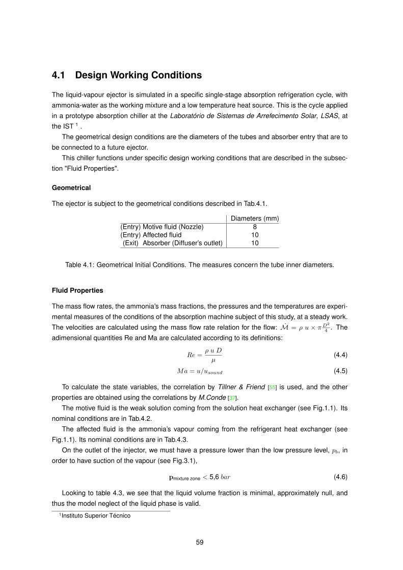
4.1 Design Working Conditions
The liquid-vapour ejector is simulated in a specific single-stage absorption refrigeration cycle, with
ammonia-water as the working mixture and a low temperature heat source. This is the cycle applied
in a prototype absorption chiller at the Laboratório de Sistemas de Arrefecimento Solar, LSAS, at
the IST 1 .
The geometrical design conditions are the diameters of the tubes and absorber entry that are to
be connected to a future ejector.
This chiller functions under specific design working conditions that are described in the subsec-
tion "Fluid Properties".
Geometrical
The ejector is subject to the geometrical conditions described in Tab.4.1.
Diameters (mm)(Entry) Motive fluid (Nozzle) 8(Entry) Affected fluid 10(Exit) Absorber (Diffuser’s outlet) 10
Table 4.1: Geometrical Initial Conditions. The measures concern the tube inner diameters.
Fluid Properties
The mass flow rates, the ammonia’s mass fractions, the pressures and the temperatures are experi-
mental measures of the conditions of the absorption machine subject of this study, at a steady work.
The velocities are calculated using the mass flow rate relation for the flow: M = ρ u × πD2
4 . The
adimensional quantities Re and Ma are calculated according to its definitions:
Re =ρ u D
µ(4.4)
Ma = u/usound (4.5)
To calculate the state variables, the correlation by Tillner & Friend [55] is used, and the other
properties are obtained using the correlations by M.Conde [37].
The motive fluid is the weak solution coming from the solution heat exchanger (see Fig.1.1). Its
nominal conditions are in Tab.4.2.
The affected fluid is the ammonia’s vapour coming from the refrigerant heat exchanger (see
Fig.1.1). Its nominal conditions are in Tab.4.3.
On the outlet of the injector, we must have a pressure lower than the low pressure level, pb, in
order to have suction of the vapour (see Fig.3.1),
pmixture zone < 5,6 bar (4.6)
Looking to table 4.3, we see that the liquid volume fraction is minimal, approximately null, and
thus the model neglect of the liquid phase is valid.1Instituto Superior Técnico
59
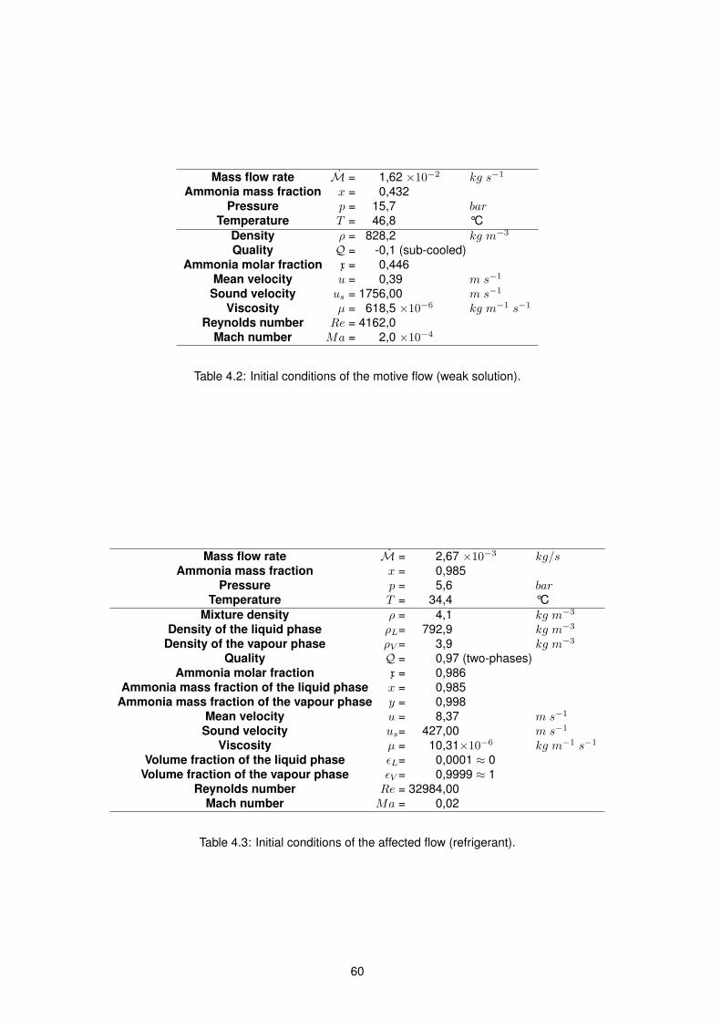
Mass flow rate M = 1,62 ×10⁻² kg s−1
Ammonia mass fraction x = 0,432Pressure p = 15,7 bar
Temperature T = 46,8 °CDensity ρ = 828,2 kg m−3
Quality Q = -0,1 (sub-cooled)Ammonia molar fraction x = 0,446
Mean velocity u = 0,39 m s−1
Sound velocity us = 1756,00 m s−1
Viscosity µ = 618,5 ×10⁻⁶ kg m−1 s−1
Reynolds number Re = 4162,0Mach number Ma = 2,0 ×10⁻⁴
Table 4.2: Initial conditions of the motive flow (weak solution).
Mass flow rate M = 2,67 ×10⁻³ kg/sAmmonia mass fraction x = 0,985
Pressure p = 5,6 barTemperature T = 34,4 °C
Mixture density ρ = 4,1 kg m−3
Density of the liquid phase ρL= 792,9 kg m−3
Density of the vapour phase ρV = 3,9 kg m−3
Quality Q = 0,97 (two-phases)Ammonia molar fraction x = 0,986
Ammonia mass fraction of the liquid phase x = 0,985Ammonia mass fraction of the vapour phase y = 0,998
Mean velocity u = 8,37 m s−1
Sound velocity us= 427,00 m s−1
Viscosity µ = 10,31×10⁻⁶ kg m−1 s−1
Volume fraction of the liquid phase εL= 0,0001 ≈ 0Volume fraction of the vapour phase εV = 0,9999 ≈ 1
Reynolds number Re = 32984,00Mach number Ma = 0,02
Table 4.3: Initial conditions of the affected flow (refrigerant).
60
Chapter 5
Results and Discussion of theSimulations
5.1 Nozzle
If we ignore the energy losses and irreversibilities, we can simplify Eq.(3.23) into the Bernoulli equa-
tion:p2 − p1
ρ+
12(u2
2 − u21
)= 0 (5.1)
This is useful to obtain an estimative of the range of values where the results are expected to lie.
Such an useful estimate is an upper bound of the velocities possible to obtain by acceleration of the
motive fluid in the interior nozzle. To obtain an upper bound, a pseudo-fluid is considered with the
property of remaining incompressible and not changing phase until it reaches zero pressure. Once at
zero pressure, there is no more pressure energy to convert to kinetic energy, and the correspondent
velocity is the maximum velocity for the pseudo-fluid (and thus an upper bound velocity for the motive
fluid). From Eq.(5.1), we have (using values from Tab.4.2):
umax =√
2 pρ
+ u2 = 61, 57 m/s (5.2)
Similar calculations were made for the pressure at which the motive fluid started to change phase
within the working conditions of the study, to confirm the validity of the simulation results.
The interior nozzle flow was simulated for the design and inlet working conditions in Tables 4.1
and 4.2, respectively. The motive flow pressure variation function of the decreasing diameter along
the nozzle length is presented in Fig.5.1(a) for a flow model with friction and without friction. It is
observed that the Bernoulli’s equation is a satisfactory model of the energy flow for low acceleration,
however, near the outlet of the nozzle, where the flow’s acceleration increases (see Fig.5.2), the
impact of the friction on the flow becomes sizable, lowering the outlet pressure.
It was observed that the flow turns into turbulent inside the diffuser, as expected from its accel-
eration.
Fig.5.1(b) presents more detailed results for the pressure variation around the desired low pres-
sure for the affected fluid, until the beginning of phase change.
It is noted a very high sensibility of the pressure to the diameter variation at the outlet, which
imply greater care in manufacturing the nozzle, in order to be at the desired working conditions.
61
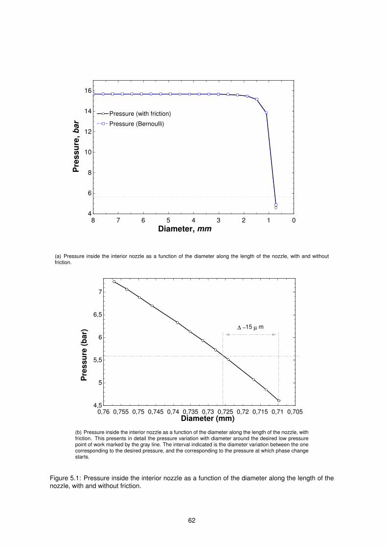
File:C:\Documents and Settings\Dingo\Desktop\Projecto\Tese\F\Inj.EES 25-05-2009 16:00:10 Page 1
EES Ver. 8.186: #1667: For use only by students and faculty at the ICIST - Instituto Superior Tecnico, Lisbon, Portugal
0123456784
6
8
10
12
14
16
Diameter, mm
Pre
ss
ure
, b
ar
Pressure (with friction)Pressure (with friction)
Pressure (Bernoulli)Pressure (Bernoulli)
(a) Pressure inside the interior nozzle as a function of the diameter along the length of the nozzle, with and withoutfriction.
File:C:\Documents and Settings\Dingo\Desktop\Projecto\Tese\F\Inj.EES 27-04-2009 12:45:01 Page 1
EES Ver. 8.186: #1667: For use only by students and faculty at the ICIST - Instituto Superior Tecnico, Lisbon, Portugal
0,7050,710,7150,720,7250,730,7350,740,7450,750,7550,764,5
5
5,5
6
6,5
7
Diameter (mm)
Pre
ss
ure
(b
ar)
! "15 µ m
(b) Pressure inside the interior nozzle as a function of the diameter along the length of the nozzle, withfriction. This presents in detail the pressure variation with diameter around the desired low pressurepoint of work marked by the gray line. The interval indicated is the diameter variation between the onecorresponding to the desired pressure, and the corresponding to the pressure at which phase changestarts.
Figure 5.1: Pressure inside the interior nozzle as a function of the diameter along the length of thenozzle, with and without friction.
62
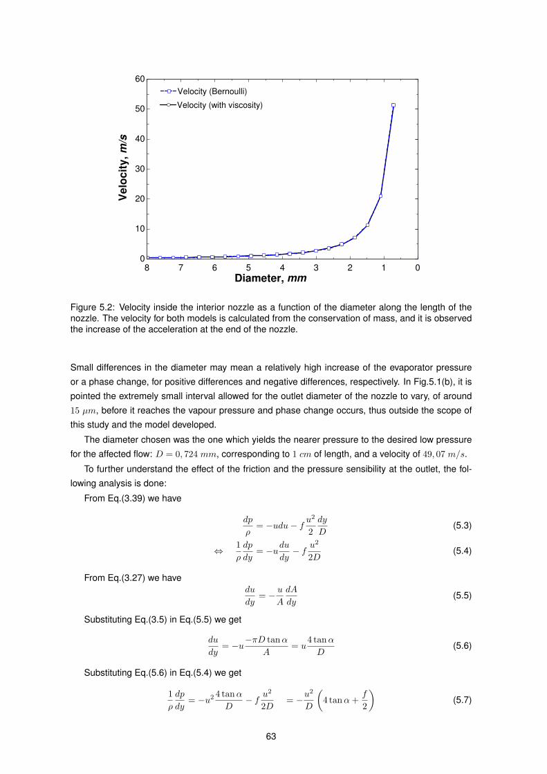
File:C:\Documents and Settings\Dingo\Desktop\Projecto\Tese\F\Inj.EES 27-04-2009 13:08:51 Page 2
EES Ver. 8.186: #1667: For use only by students and faculty at the ICIST - Instituto Superior Tecnico, Lisbon, Portugal
0123456780
10
20
30
40
50
60
Diameter, mm
Ve
loc
ity
, m
/s
Velocity (with viscosity)Velocity (with viscosity)
Velocity (Bernoulli)Velocity (Bernoulli)
0123456780
10000
20000
30000
40000
50000
Diameter, mm
Re
Reynolds Number (with viscosity)Reynolds Number (with viscosity)
Reynolds Number (with bernoulli as the conservation of energy equation)Reynolds Number (with bernoulli as the conservation of energy equation)
Figure 5.2: Velocity inside the interior nozzle as a function of the diameter along the length of thenozzle. The velocity for both models is calculated from the conservation of mass, and it is observedthe increase of the acceleration at the end of the nozzle.
Small differences in the diameter may mean a relatively high increase of the evaporator pressure
or a phase change, for positive differences and negative differences, respectively. In Fig.5.1(b), it is
pointed the extremely small interval allowed for the outlet diameter of the nozzle to vary, of around
15 µm, before it reaches the vapour pressure and phase change occurs, thus outside the scope of
this study and the model developed.
The diameter chosen was the one which yields the nearer pressure to the desired low pressure
for the affected flow: D = 0, 724 mm, corresponding to 1 cm of length, and a velocity of 49, 07 m/s.
To further understand the effect of the friction and the pressure sensibility at the outlet, the fol-
lowing analysis is done:
From Eq.(3.39) we have
dp
ρ= −udu− f u
2
2dy
D(5.3)
⇔ 1ρ
dp
dy= −udu
dy− f u
2
2D(5.4)
From Eq.(3.27) we havedu
dy= − u
A
dA
dy(5.5)
Substituting Eq.(3.5) in Eq.(5.5) we get
du
dy= −u−πD tanα
A= u
4 tanαD
(5.6)
Substituting Eq.(5.6) in Eq.(5.4) we get
1ρ
dp
dy= −u2 4 tanα
D− f u
2
2D= −u
2
D
(4 tanα+
f
2
)(5.7)
63
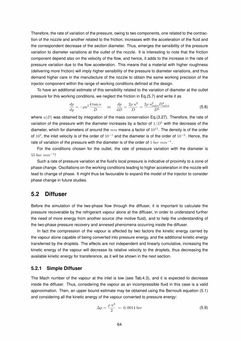
Therefore, the rate of variation of the pressure, owing to two components, one related to the contrac-
tion of the nozzle and another related to the friction, increases with the acceleration of the fluid and
the correspondent decrease of the section diameter. Thus, emerges the sensibility of the pressure
variation to diameter variations at the outlet of the nozzle. It is interesting to note that the friction
component depend also on the velocity of the flow, and hence, it adds to the increase in the rate of
pressure variation due to the flow acceleration. This means that a material with higher roughness
(delivering more friction) will imply higher sensibility of the pressure to diameter variations, and thus
demand higher care in the manufacture of the nozzle to obtain the same working precision of the
injector component within the range of working conditions defined at the design.
To have an additional estimate of this sensibility related to the variation of diameter at the outlet
pressure for this working conditions, we neglect the friction in Eq.(5.7) and write it as
dp
dy= −ρu2 4 tanα
D⇔ dp
dD=
2ρ u2
D=
2ρ u2inletD
4inlet
D5(5.8)
where u(D) was obtained by integration of the mass conservation Eq.(3.27). Therefore, the rate of
variation of the pressure with the diameter increases by a factor of 1/D5 with the decrease of the
diameter, which for diameters of around the mm means a factor of 1015. The density is of the order
of 103, the inlet velocity is of the order of 10−1 and the diameter is of the order of 10−2. Hence, the
rate of variation of the pressure with the diameter is of the order of 1 bar mm−1.
For the conditions chosen for the outlet, the rate of pressure variation with the diameter is
55 bar mm−1!
Such a rate of pressure variation at the fluid’s local pressure is indicative of proximity to a zone of
phase change. Oscillations on the working conditions leading to higher acceleration in the nozzle will
lead to change of phase. It might thus be favourable to expand the model of the injector to consider
phase change in future studies.
5.2 Diffuser
Before the simulation of the two-phase flow through the diffuser, it is important to calculate the
pressure recoverable by the refrigerant vapour alone at the diffuser, in order to understand further
the need of more energy from another source (the motive fluid), and to help the understanding of
the two-phase pressure recovery and annexed phenomena occurring inside the diffuser.
In fact the compression of the vapour is affected by two factors the kinetic energy carried by
the vapour alone capable of being converted into pressure energy, and the additional kinetic energy
transferred by the droplets. The effects are not independent and linearly cumulative, increasing the
kinetic energy of the vapour will decrease its relative velocity to the droplets, thus decreasing the
available kinetic energy for transference, as it will be shown in the next section.
5.2.1 Simple Diffuser
The Mach number of the vapour at the inlet is low (see Tab.4.3), and it is expected to decrease
inside the diffuser. Thus, considering the vapour as an incompressible fluid in this case is a valid
approximation. Then, an upper bound estimate may be obtained using the Bernoulli equation (5.1)
and considering all the kinetic energy of the vapour converted to pressure energy:
∆p =ρ u2
2= 0, 0014 bar (5.9)
64
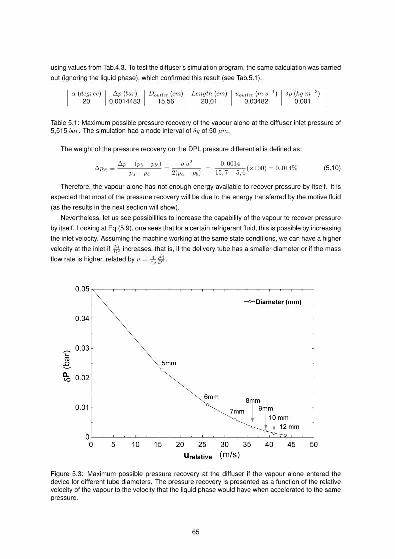
using values from Tab.4.3. To test the diffuser’s simulation program, the same calculation was carried
out (ignoring the liquid phase), which confirmed this result (see Tab.5.1).
α (degree) ∆p (bar) Doutlet (cm) Length (cm) uoutlet (m s−1) δρ (kg m−3)20 0,0014483 15,56 20,01 0,03482 0,001
Table 5.1: Maximum possible pressure recovery of the vapour alone at the diffuser inlet pressure of5,515 bar. The simulation had a node interval of δy of 50 µm.
The weight of the pressure recovery on the DPL pressure differential is defined as:
∆p% ≡∆p− (pb − pb′)
pa − pb=
ρ u2
2(pa − pb)=
0, 001415, 7− 5, 6
(×100) = 0, 014% (5.10)
Therefore, the vapour alone has not enough energy available to recover pressure by itself. It is
expected that most of the pressure recovery will be due to the energy transferred by the motive fluid
(as the results in the next section will show).
Nevertheless, let us see possibilities to increase the capability of the vapour to recover pressure
by itself. Looking at Eq.(5.9), one sees that for a certain refrigerant fluid, this is possible by increasing
the inlet velocity. Assuming the machine working at the same state conditions, we can have a higher
velocity at the inlet if MD2 increases, that is, if the delivery tube has a smaller diameter or if the mass
flow rate is higher, related by u = 4πρMD2 .
Figure 5.3: Maximum possible pressure recovery at the diffuser if the vapour alone entered thedevice for different tube diameters. The pressure recovery is presented as a function of the relativevelocity of the vapour to the velocity that the liquid phase would have when accelerated to the samepressure.
65
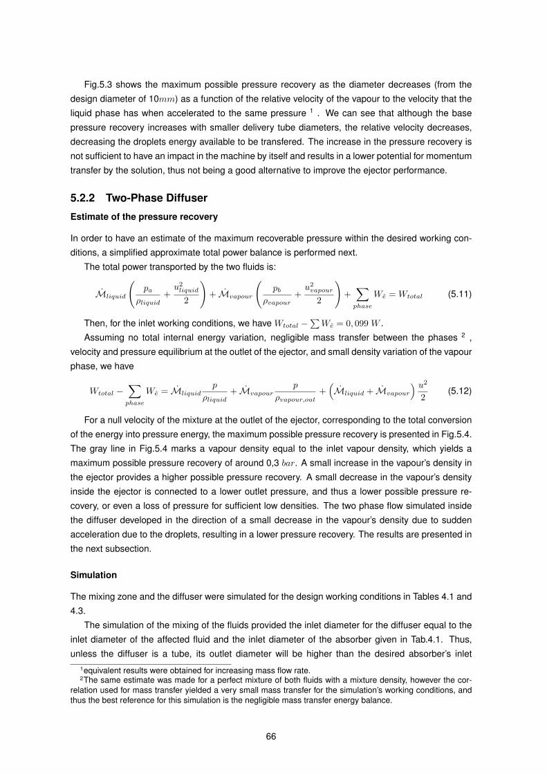
Fig.5.3 shows the maximum possible pressure recovery as the diameter decreases (from the
design diameter of 10mm) as a function of the relative velocity of the vapour to the velocity that the
liquid phase has when accelerated to the same pressure 1 . We can see that although the base
pressure recovery increases with smaller delivery tube diameters, the relative velocity decreases,
decreasing the droplets energy available to be transfered. The increase in the pressure recovery is
not sufficient to have an impact in the machine by itself and results in a lower potential for momentum
transfer by the solution, thus not being a good alternative to improve the ejector performance.
5.2.2 Two-Phase Diffuser
Estimate of the pressure recovery
In order to have an estimate of the maximum recoverable pressure within the desired working con-
ditions, a simplified approximate total power balance is performed next.
The total power transported by the two fluids is:
Mliquid
(pa
ρliquid+u2liquid
2
)+ Mvapour
(pb
ρvapour+u2vapour
2
)+∑phase
We = Wtotal (5.11)
Then, for the inlet working conditions, we have Wtotal −∑We = 0, 099 W .
Assuming no total internal energy variation, negligible mass transfer between the phases 2 ,
velocity and pressure equilibrium at the outlet of the ejector, and small density variation of the vapour
phase, we have
Wtotal −∑phase
We = Mliquidp
ρliquid+ Mvapour
p
ρvapour,out+(Mliquid + Mvapour
) u2
2(5.12)
For a null velocity of the mixture at the outlet of the ejector, corresponding to the total conversion
of the energy into pressure energy, the maximum possible pressure recovery is presented in Fig.5.4.
The gray line in Fig.5.4 marks a vapour density equal to the inlet vapour density, which yields a
maximum possible pressure recovery of around 0,3 bar. A small increase in the vapour’s density in
the ejector provides a higher possible pressure recovery. A small decrease in the vapour’s density
inside the ejector is connected to a lower outlet pressure, and thus a lower possible pressure re-
covery, or even a loss of pressure for sufficient low densities. The two phase flow simulated inside
the diffuser developed in the direction of a small decrease in the vapour’s density due to sudden
acceleration due to the droplets, resulting in a lower pressure recovery. The results are presented in
the next subsection.
Simulation
The mixing zone and the diffuser were simulated for the design working conditions in Tables 4.1 and
4.3.
The simulation of the mixing of the fluids provided the inlet diameter for the diffuser equal to the
inlet diameter of the affected fluid and the inlet diameter of the absorber given in Tab.4.1. Thus,
unless the diffuser is a tube, its outlet diameter will be higher than the desired absorber’s inlet1equivalent results were obtained for increasing mass flow rate.2The same estimate was made for a perfect mixture of both fluids with a mixture density, however the cor-
relation used for mass transfer yielded a very small mass transfer for the simulation’s working conditions, andthus the best reference for this simulation is the negligible mass transfer energy balance.
66
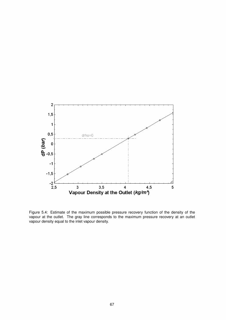
Figure 5.4: Estimate of the maximum possible pressure recovery function of the density of thevapour at the outlet. The gray line corresponds to the maximum pressure recovery at an outletvapour density equal to the inlet vapour density.
67
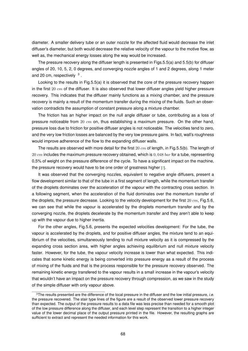
diameter. A smaller delivery tube or an outer nozzle for the affected fluid would decrease the inlet
diffuser’s diameter, but both would decrease the relative velocity of the vapour to the motive flow, as
well as, the mechanical energy losses along the way would be increased.
The pressure recovery along the diffuser length is presented in Figs.5.5(a) and 5.5(b) for diffuser
angles of 20, 10, 5, 2, 0 degrees, and converging nozzle angles of 1 and 2 degrees, along 1 meter
and 20 cm, respectively 3 .
Looking to the results in Fig.5.5(a) it is observed that the core of the pressure recovery happen
in the first 20 cm of the diffuser. It is also observed that lower diffuser angles yield higher pressure
recovery. This indicates that the diffuser mainly functions as a mixing chamber, and the pressure
recovery is mainly a result of the momentum transfer during the mixing of the fluids. Such an obser-
vation contradicts the assumption of constant pressure along a mixture chamber.
The friction has an higher impact on the null angle diffuser or tube, contributing as a loss of
pressure noticeable from 20 cm on, thus establishing a maximum pressure. On the other hand,
pressure loss due to friction for positive diffuser angles is not noticeable. The velocities tend to zero,
and the very low friction losses are balanced by the very low pressure gains. In fact, wall’s roughness
would improve adherence of the flow to the expanding diffuser walls.
The results are observed with more detail for the first 20 cm of length, in Fig.5.5(b). The length of
20 cm includes the maximum pressure recovery obtained, which is 0, 048 bar for a tube, representing
0,5% of weight on the pressure difference of the cycle. To have a significant impact on the machine,
the pressure recovery would have to be one order of greatness higher [7].
It was observed that the converging nozzles, equivalent to negative angle diffusers, present a
flow development similar to that of the tube in a first segment of length, while the momentum transfer
of the droplets dominates over the acceleration of the vapour with the contracting cross section. In
a following segment, when the acceleration of the fluid dominates over the momentum transfer of
the droplets, the pressure decrease. Looking to the velocity development for the first 20 cm, Fig.5.6,
we can see that while the vapour is accelerated by the droplets momentum transfer and by the
converging nozzle, the droplets decelerate by the momentum transfer and they aren’t able to keep
up with the vapour due to higher inertia.
For the other angles, Fig.5.6, presents the expected velocities development: For the tube, the
vapour is accelerated by the droplets, and for positive diffuser angles, the mixture tend to an equi-
librium of the velocities, simultaneously tending to null mixture velocity as it is compressed by the
expanding cross section area, with higher angles achieving equilibrium and null mixture velocity
faster. However, for the tube, the vapour velocity increase is lower than what expected. This indi-
cates that some kinetic energy is being converted into pressure energy as a result of the process
of mixing of the fluids and that is the process responsible for the pressure recovery observed. The
remaining kinetic energy transfered to the vapour results in a small increase in the vapour’s velocity
that wouldn’t have an impact on the pressure recovery through compression, as we saw in the study
of the simple diffuser with only vapour above.
3The results presented are the difference of the local pressure in the diffuser and the low initial pressure, i.e.the pressure recovered. The stair type lines of the figure are a result of the observed lower pressure recoverythan expected. The output of the pressure results to a data file was less precise than needed for a smooth plotof the low pressure difference along the diffuser, and each level step represent the transition to a higher integervalue of the lower decimal place of the output pressure printed in the file. However, the resulting graphs aresufficient to extract and represent the needed information for this work.
68
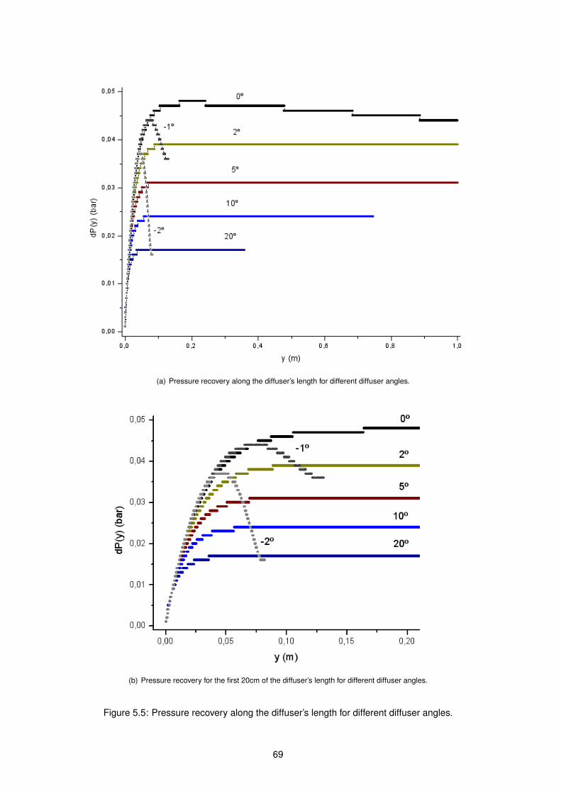
(a) Pressure recovery along the diffuser’s length for different diffuser angles.
(b) Pressure recovery for the first 20cm of the diffuser’s length for different diffuser angles.
Figure 5.5: Pressure recovery along the diffuser’s length for different diffuser angles.
69
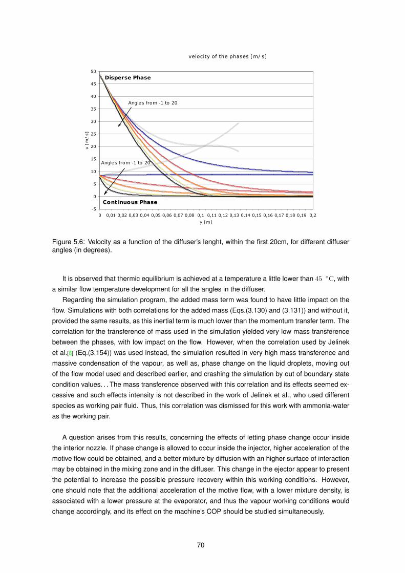
velocity of the phases [m/ s]
-5
0
5
10
15
20
25
30
35
40
45
50
0 0,01 0,02 0,03 0,04 0,05 0,06 0,07 0,08 0,1 0,11 0,12 0,13 0,14 0,15 0,16 0,17 0,18 0,19 0,2
y [m]
u [
m/
s]
Angles from -1 to 20
Angles from -1 to 20
Disperse Phase
Cont inuous Phase
Figure 5.6: Velocity as a function of the diffuser’s lenght, within the first 20cm, for different diffuserangles (in degrees).
It is observed that thermic equilibrium is achieved at a temperature a little lower than 45 ◦C, with
a similar flow temperature development for all the angles in the diffuser.
Regarding the simulation program, the added mass term was found to have little impact on the
flow. Simulations with both correlations for the added mass (Eqs.(3.130) and (3.131)) and without it,
provided the same results, as this inertial term is much lower than the momentum transfer term. The
correlation for the transference of mass used in the simulation yielded very low mass transference
between the phases, with low impact on the flow. However, when the correlation used by Jelinek
et al.[6] (Eq.(3.154)) was used instead, the simulation resulted in very high mass transference and
massive condensation of the vapour, as well as, phase change on the liquid droplets, moving out
of the flow model used and described earlier, and crashing the simulation by out of boundary state
condition values. . . The mass transference observed with this correlation and its effects seemed ex-
cessive and such effects intensity is not described in the work of Jelinek et al., who used different
species as working pair fluid. Thus, this correlation was dismissed for this work with ammonia-water
as the working pair.
A question arises from this results, concerning the effects of letting phase change occur inside
the interior nozzle. If phase change is allowed to occur inside the injector, higher acceleration of the
motive flow could be obtained, and a better mixture by diffusion with an higher surface of interaction
may be obtained in the mixing zone and in the diffuser. This change in the ejector appear to present
the potential to increase the possible pressure recovery within this working conditions. However,
one should note that the additional acceleration of the motive flow, with a lower mixture density, is
associated with a lower pressure at the evaporator, and thus the vapour working conditions would
change accordingly, and its effect on the machine’s COP should be studied simultaneously.
70
Chapter 6
Conclusions
The TPL cycle is specially suited for solar heated refrigeration systems as it permits a higher Co-
efficient of Performance (COP) at the lower working temperatures adequate for the solar collectors
panels.
The ejector-absorption cycle, using a liquid-vapour ejector to recover pressure, has revealed
to be promising form of this cycle, for various working mixtures, however the use of a mixture of
ammonia-water needed to be conveniently studied. The ejector device reveals numerous advan-
tages both economically and functionally, featuring simplicity and low maintenance need, and the
use of energy otherwise lost in the cycle.
In view of changing the current single-stage DPL absorption experimental chiller (in the LSAS
Laboratory at IST) working with a low temperature heat source, into a TPL ejector-absorption chiller
in the future, the limits of the application of a liquid-vapour ejector at the absorber inlet were studied
to function within the design working conditions of the current chiller, using an ammonia-water work-
ing mixture, with the aim of finding the pressure recoverable and the design associated. The study
consisted of two phases: construction of a flow model for a liquid-vapour ejector and simulation of
the liquid-vapour ejector at the chiller’s design working conditions.
A new two-phase flow model was derived for a liquid-vapour ejector without phase change inside
the nozzle. The model adds to previous ejectors models used in this kind of simulations the me-
chanical energy losses due to friction with the wall, which reduce the available energy for pressure
recovery through dissipation along the way, particularly yielding a maximum on the tube’s pressure
recovery profile. The diffuser’s model includes the mass, momentum and energy transfer between
the phases (for different kinetic regimes), as well as inertial forces associated with the flow. Beside
this quantities also considered in previous models, the new model takes into account the vapour’s
refrigerant mass fraction in the calculations of its physical and state properties, as well as the change
of the mass fraction of the phases and the variation of the droplet diameter with the mass transfer-
ence.
A simulation program was then created based on the ejector’s model. The program was used to
study the pressure recovery possible for an ejector working in an ejector-absorption cycle with low
temperature heat source and a binary mixture of ammonia-water, adding new simulation results for
this specific type of ejector-absorption cycles to the results of ejector-absorption cycles that exist in
literature. The simulation of the ejector was divided in two: the simulation of the injector, and the
simulation of the diffuser.
71
From the results of the simulation of the injector, an appropriate design for the interior nozzle was
chosen in order to have the desired affected fluid’s working conditions at the outlet. The appropriate
nozzle should have an inlet and outlet diameters of 8 and 0,724 mm, respectively, and a length of 1
cm. It is also preferred low surface roughness, to minimize the friction losses near the outlet, and an
outlet finish adequate to diffuse uniformly the exiting droplets.
However, it was observed very high sensibility of the pressure to outlet diameters variations, what
implies great care in the manufacture of the nozzle in order to function within the desired working
conditions. An extremely small variation of 15 µm in the outlet diameter of the nozzle is sufficient to
cause phase change inside the nozzle, which is outside the work regime for a liquid-vapour ejector,
subject of this study, which assumes a liquid phase exiting the nozzle. It also means a high sensibility
of the outlet conditions to changes in the inlet conditions.
The diffuser program was used to simulate the flow of the vapour alone. It confirmed that the
vapour isn’t able to recover sufficient pressure by itself. When compared to following simulations,
the ejector was able to increase the pressure recovery by a factor of 10. Increasing the power trans-
ported by the vapour alone do not predict an improvement in the ejector’s performance, because
increasing the pressure recovery possible by the vapour alone decreases the useful power available
for transference by the droplets, and it is previewed that the low intensity possible to achieve as little
impact on the device as well as in the cycle. It was concluded that main source of pressure recovery
is the energy carried by the motive fluid.
From the results of the simulation of the diffuser, it was concluded that the pressure recovery
possible increased with the decrease of the diffuser angle, which means that the pressure recovery
is mainly due to the mixing and momentum transfer between the two fluids. It was concluded that
in this cycle the diffuser’s main function is as a mixing chamber. The simulation yielded a maximum
pressure recovery possible of 0,05 bar for a tube with a 20cm length, which is too low to have a
noticeable impact on the machine’s efficiency.
The simulation also provided useful insight on the diffuser’s multiphase flow. The introduction
of the friction made possible to account for pressure loss with the length, resulting in a well defined
maximum pressure recovery point for the tube. It was concluded that the dominant force for pressure
recovery in such systems is the momentum transfer, and that the assumption of constant pressure
along the length of a mixing chamber is not valid.
It was concluded that it is favorable to expand the model of the liquid-vapour ejector to include
phase change inside the injector, for the case of using ammonia-water as the working mixture.
Such a liquid-vapour ejector model that includes phase change in the nozzle have not been
read neither referred in the bibliography. Therefore, the prosecution of the work initiated in this
dissertation, includes the derivation of a new theoretical flow model for the liquid-vapour ejector
including phase change at the injector, as well as its experimental validation.
72
References
[1] Pons M. et al. Thermodynamic based comparison of sorption systems for cooling and heat
pumping. International Journal of Refrigeration, 22(1):5–7, 1999.
[2] L. Filipe Mendes, M. Collares-Pereira, and F. Ziegler. Supply of cooling and heating with solar
assisted absorption heat pumps: an energetic approach. International Journal of Refrigeration,
21(2):116–125, March 1998.
[3] Shenyi Wu and Ian W. Eames. Innovations in vapour-absorption cycles. Applied Energy,
66(3):251–266, July 2000.
[4] Pongsid Srikhirin, Satha Aphornratana, and Supachart Chungpaibulpatana. A review of absorp-
tion refrigeration technologies. Renewable and Sustainable Energy Reviews, 5(4):343–372,
December 2001.
[5] Keith E. Herold, Reinhard Radermacher, and Sanford A. Klein. Absorption Chillers and Heat
Pumps. Number 0-8493-9427-9. CRC Press, Inc., 1996.
[6] A. Levy, M. Jelinek, and I. Borde. Performance of a triple-pressure-level absorption cycle with
r125-n,n’-dimethylethylurea. Applied Energy, 71:171–189, 2002.
[7] A. C. Gonçalves. Estudo e Concepção de um Ejector para uma Máquina de Absorção com o
par NH3/H2O. Instituto Superior Técnico - UTL, Lisboa, Portugal, Setembro 2006.
[8] C.E. Strickland Landis Kneass. Practice and Theory of the Injector. John Wiley & Sons, 2nd
edition, 1898.
[9] George N. Nissenson. Pratical Treatise on INJECTORS as Feeders of Steam Boilers for the use
of Master Mechanics and Engineers in charge of Locomotive, Marine and Stationary Boilers.
Published by the Author, New York, 1890.
[10] http://en.wikipedia.org/wiki/injector, 8 February 2009.
[11] M.H. Résal. Recherches Theoriques sur les effects mécaniques de L’Injecteur Automoteur de
M. Giffard. Dunod, Éditeur, Paris, 1862.
[12] Absorption refrigeration system with multiple generator stages - patent 3717007, February
1973.
[13] H. Chung, M.H. Huor, M. Prevost, and R. Bugarel. Domestic heating application of an absorp-
tion heat-pump. In Directly fired heat pumps, Procs. Int. Conf., number 2.2. Uni. Of Bristol,
1984.
73
[14] L. T. Chen. A new ejector-absorber cycle to improve the cop of an absorption refrigeration
system. Applied Energy, 30(1):37–51, 1988.
[15] A. Levy, M. Jelinek, and I. Borde. Numerical study on the design parameters of a jet ejector for
absorption systems. Applied Energy, 72:467–478, 2002.
[16] N. C. Daltrophe, M. Jelinek, and I. Borde. Heat and mass transfer in a two-phase flow of a
binary solution and a gas. In Heat Transfer 1994: 10th International Conference : Papers.,
pages 299–304. IMechE, Institution of Chemical Engineers, Taylor & Francis, 1994.
[17] N. Daltrophe, M. Jelinek, and I. Borde. Heat and mass transfer in a jet ejector for absorption
systems. ASME, International Absorption Heat Pump Conference, pages 327–332, 1994.
[18] Satha Aphornratana and Ian W. Eames. Experimental investigation of a combined ejector-
absorption regrigerator. International Journal of Energy Research, 22:195–207, 1998.
[19] S. Aphornratana. Theoretical and experimental investigation of a combined ejector-absorption
refrigerator. In:(23rd edn.), PhD thesis, Department of Mechanical and Process Engineering,
University of Sheffield, UK, 1994.
[20] I.W.Eames and S. Aphornratana. A novel ejector/absorption cycle refrigerator for building air
conditioning. In Proc. CIBSE National Conference, Eastbourne, 1995.
[21] I.W.Eames, M. Georghiades, R. J. Tucker, S. Aphornratana, and S. Wu. Combined ejector-
absorption cycle technology for gas-fired air conditioning. In Proc. Absorption 96, volume 1,
pages 201–8, 17-20 September 1996.
[22] Da-Wen Sun, Ian W. Earnes, and Satha Aphornratana. Evaluation of a novel combined ejector-
absorption refrigeration cycle - i: computer simulation. International Journal of Refrigeration,
19(3):172–180, 1996.
[23] He S et al. Progress of mathematical modeling on ejectors. Renew Sustain Energy Rev. (2008),
doi:10.1016/j.rser.2008.09.032
[24] Z. Gu, S. Feng, and Y. Yu. Absorption-ejector hybrid refrigeration cycle powered by low grade
heat. In Proc. Absorption 96 [21], pages 177–82.
[25] S. Wu and I.W.Eames. A novel absorption-recompression refrigeration cycle. Applied Thermal
Engineering, 18:1149–1157, 1998.
[26] Ian W. Eames and Shenyi Wu. A theoretical study of an innovative ejector powered absorption-
recompression cycle refrigerator. International Journal of Refrigeration, 23:475–484, 2000.
[27] J. Wang, G. Chen, and H. Jiang. Study on a solar-driven ejection absorption refrigeration cycle.
International Journal of Energy Research, 22:733–739, 1998.
[28] A. Levy, M. Jelinek, I. Borde, and F. Ziegler. Performance of an advanced absorption cycle with
r125 and different absorbents. Applied Energy, 29:2501–2515, 2004.
[29] Adnan Sözen and Mehmet Özalp. Performance improvement of absorption refrigeration system
using triple-pressure-level. Applied Thermal Engineering, 23(13):1577–1593, September 2003.
74
[30] Adnan Sözen and Mehmet Özalp. Solar-driven ejector-absorption cooling system. Applied
Energy, 80(1):97–113, January 2005.
[31] F. White. Fluid Mechanics. McGraw-Hill, 5th edition, 2003.
[32] F. Cengel. Fluid Mechanics. McGraw-Hill, 5th edition, 2003.
[33] Jr. John D. Anderson. Modern Compressible Flow with Historical Perspective. McGraw-Hill, 3rd
edition, 2003.
[34] Fluid mechanics and heat transfer, volume 2 of Heat Exchanger Design Handbook. Hemisphere
Publishing Corporation, 1983.
[35] Christopher Earls Brennen. Fundamentals of Multiphase Flow. Cambridge University Press,
2005.
[36] Frank P. Incropera and David P. Dewitt. Fundamentos de Transferência de Calor e Massa. LTC
Editora (Authorized translation from the english edition published by John Wiley & Sons, Inc.),
5th edition, 2003.
[37] M. Conde-Petit. Thermophysical properties of {NH3 + H2O} mixtures for the industrial design
of absorption refrigeration equipment. Technical report, M. Conde Engineering, Zurich, 2006.
[38] A. Fenghour, W. A. Wakeham, V. Vesovic, J. T. R. Watson, and E. Vogel. The viscosity of
ammonia. American Institute of Physics and American Chemical Society, 24(5), June 1995.
[39] A. Levy, M. Jelinek, and I. Borde. Numerical study on the design parameters of a jet ejector for
absorption systems. Applied Energy, (72):467–478, 2002.
[40] http://en.wikipedia.org/wiki/coanda_effect, January 2009.
[41] http://pt.wikipedia.org/wiki/efeito_coanda, January 2009.
[42] http://en.wikipedia.org/wiki/d’alembert’s_paradox, January 2009.
[43] George Gabriel Stokes. On the effect of the internal friction of fluids on the motion of pendulums.
Transactions of the Cambridge Philosophical Society, IX:8–106, December 1850.
[44] Carl Wilhelm Oseen. Über die stokes’sche formel, und über eine verwadte aufgabe in der
hydrodynamik. Arkiv för matematik, astronomi och fysik, VI(29), 1910.
[45] Ian Proudman and J. R. A. Pearson. Expansions at small reynolds numbers for the flow past a
sphere and a circular cylinder. Journal of Fluid Mechanics, 2(3):237–263, 1957.
[46] Sadatoshi Taneda. Experimental investigation of the wake behind a sphere at low reynolds
numbers. J. Phys. Soc. Jpn., 11:1104–1108, June 1956.
[47] L. B. Torobin and W. H. Gauvin. Fundamental aspects of solid-gas flow. Canadian J Chem Eng,
1958.
[48] W. Ranz and W. Marshall. Chem.Eng.Prog., 48(141), 1952.
[49] S. Whitaker. Forced convection heat transfer correlation for flow in pipes, past flat plates, single
cylinders, single spheres and flow in packed beds and tube bundles. AIChE journal, 18(2):361–
371, 1972.
75
[50] S. Wisniewski and T. Wisniewski. Heat Transfer. WNT, Warszawa, 2000.
[51] L. Boguslawski. Estimation of the influence of inflow turbulence on heat convection from a
sphere surface. Journal of Theoretical and Applied Mechanics, 45(3):505–511, 2007.
[52] Markku Kulmala, Timo Vesala, Jaroslav Schwartz, and Jiri Smolik. Mass transfer from a drop
- ii. theoretical analysis of temperature dependent mass flux correlation. Int. J. Heat Mass
Transfer, 38(9):1705–1708, 1995.
[53] D. I. Kolaitis and M. A. Founti. A comparative study of numerical models for eulerian-lagrangian
simulations of turbulent evaporating sprays. International Journal of Heat and Fluid Flow,
27:424–435, January 2006.
[54] S. A. Klein. EES - Engineering Equation Solver for Microsoft Windows Operating Systems.
F-Chart Software, 2008.
[55] Reiner Tillner-Roth and Daniel G. Friend. A helmoholtz free energy formulation of the ther-
modynamic properties of the mixture {Water + Ammonia}. American Institute of Physics and
American Chemical Society, 27(1), October 1998.
[56] The International Association for the Properties of Water and Steam, Gaithersburg, Mary-
land, USA. Guideline on the IAPWS Formulation 2001 for the Thermodynamic Properties of
Ammonia-Water Mixtures, September 2001.
76
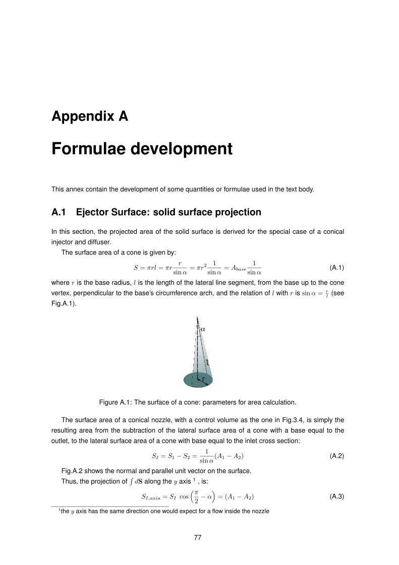
Appendix A
Formulae development
This annex contain the development of some quantities or formulae used in the text body.
A.1 Ejector Surface: solid surface projection
In this section, the projected area of the solid surface is derived for the special case of a conical
injector and diffuser.
The surface area of a cone is given by:
S = πrl = πrr
sinα= πr2
1sinα
= Abase1
sinα(A.1)
where r is the base radius, l is the length of the lateral line segment, from the base up to the cone
vertex, perpendicular to the base’s circumference arch, and the relation of l with r is sinα = rl (see
Fig.A.1).
r
l
�
Figure A.1: The surface of a cone: parameters for area calculation.
The surface area of a conical nozzle, with a control volume as the one in Fig.3.4, is simply the
resulting area from the subtraction of the lateral surface area of a cone with a base equal to the
outlet, to the lateral surface area of a cone with base equal to the inlet cross section:
SI = S1 − S2 =1
sinα(A1 −A2) (A.2)
Fig.A.2 shows the normal and parallel unit vector on the surface.
Thus, the projection of∫dS along the y axis 1 , is:
SI,axis = SI cos(π
2− α
)= (A1 −A2) (A.3)
1the y axis has the same direction one would expect for a flow inside the nozzle
77
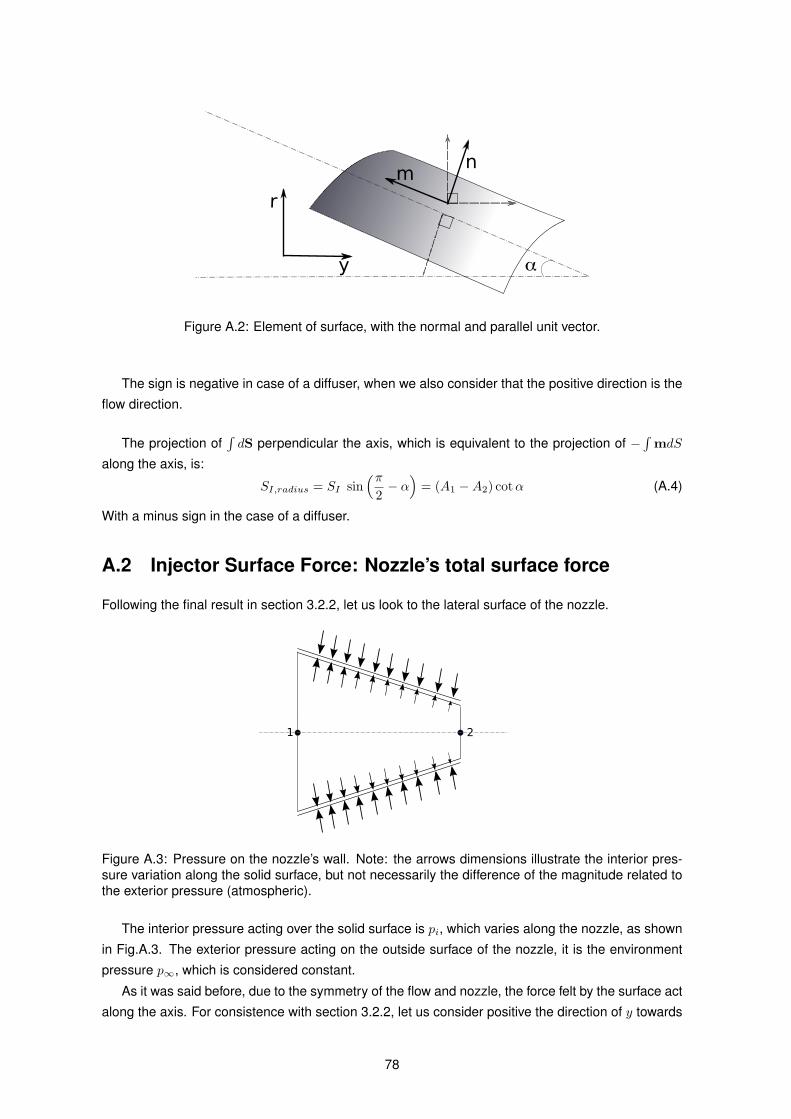
nm
�y
r
Figure A.2: Element of surface, with the normal and parallel unit vector.
The sign is negative in case of a diffuser, when we also consider that the positive direction is the
flow direction.
The projection of∫dS perpendicular the axis, which is equivalent to the projection of −
∫mdS
along the axis, is:
SI,radius = SI sin(π
2− α
)= (A1 −A2) cotα (A.4)
With a minus sign in the case of a diffuser.
A.2 Injector Surface Force: Nozzle’s total surface force
Following the final result in section 3.2.2, let us look to the lateral surface of the nozzle.
1 2
Figure A.3: Pressure on the nozzle’s wall. Note: the arrows dimensions illustrate the interior pres-sure variation along the solid surface, but not necessarily the difference of the magnitude related tothe exterior pressure (atmospheric).
The interior pressure acting over the solid surface is pi, which varies along the nozzle, as shown
in Fig.A.3. The exterior pressure acting on the outside surface of the nozzle, it is the environment
pressure p∞, which is considered constant.
As it was said before, due to the symmetry of the flow and nozzle, the force felt by the surface act
along the axis. For consistence with section 3.2.2, let us consider positive the direction of y towards
78
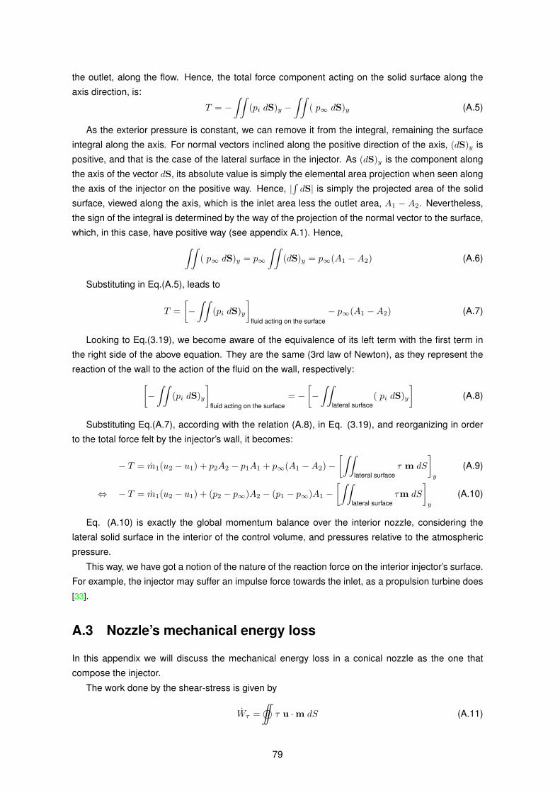
the outlet, along the flow. Hence, the total force component acting on the solid surface along the
axis direction, is:
T = −∫∫
(pi dS)y −∫∫
( p∞ dS)y (A.5)
As the exterior pressure is constant, we can remove it from the integral, remaining the surface
integral along the axis. For normal vectors inclined along the positive direction of the axis, (dS)y is
positive, and that is the case of the lateral surface in the injector. As (dS)y is the component along
the axis of the vector dS, its absolute value is simply the elemental area projection when seen along
the axis of the injector on the positive way. Hence, |∫dS| is simply the projected area of the solid
surface, viewed along the axis, which is the inlet area less the outlet area, A1 − A2. Nevertheless,
the sign of the integral is determined by the way of the projection of the normal vector to the surface,
which, in this case, have positive way (see appendix A.1). Hence,∫∫( p∞ dS)y = p∞
∫∫(dS)y = p∞(A1 −A2) (A.6)
Substituting in Eq.(A.5), leads to
T =[−∫∫
(pi dS)y
]fluid acting on the surface
− p∞(A1 −A2) (A.7)
Looking to Eq.(3.19), we become aware of the equivalence of its left term with the first term in
the right side of the above equation. They are the same (3rd law of Newton), as they represent the
reaction of the wall to the action of the fluid on the wall, respectively:[−∫∫
(pi dS)y
]fluid acting on the surface
= −[−∫∫
lateral surface( pi dS)y
](A.8)
Substituting Eq.(A.7), according with the relation (A.8), in Eq. (3.19), and reorganizing in order
to the total force felt by the injector’s wall, it becomes:
− T = m1(u2 − u1) + p2A2 − p1A1 + p∞(A1 −A2)−[∫∫
lateral surfaceτ m dS
]y
(A.9)
⇔ − T = m1(u2 − u1) + (p2 − p∞)A2 − (p1 − p∞)A1 −[∫∫
lateral surfaceτm dS
]y
(A.10)
Eq. (A.10) is exactly the global momentum balance over the interior nozzle, considering the
lateral solid surface in the interior of the control volume, and pressures relative to the atmospheric
pressure.
This way, we have got a notion of the nature of the reaction force on the interior injector’s surface.
For example, the injector may suffer an impulse force towards the inlet, as a propulsion turbine does
[33].
A.3 Nozzle’s mechanical energy loss
In this appendix we will discuss the mechanical energy loss in a conical nozzle as the one that
compose the injector.
The work done by the shear-stress is given by
Wτ =©∫∫
τ u ·m dS (A.11)
79
The work done by the shear-stress and friction in nozzles is usually studied as a global mechani-
cal energy loss coefficient, using experimental correlations. Factories usually deliver the nozzle with
the correspondent experimental correlation for the pressure losses.
Reliable correlations and formulae for the mechanical energy losses in tubes and sudden con-
traction are frequently used nowadays [31] [32] [34].
The mechanical energy loss per unit of mass in a tube is given by:
wf = fu2
2L
D(A.12)
wf =M fu2
2L
D(A.13)
where f is the Darcy friction factor, u is the mean inlet velocity, L is the tube’s lenght, D is the tube’s
diameter, andM is the mean mass flow rate inside the tube.
The mechanical energy loss per unit of mass in a sudden contraction is given by [31]:
wSC =
(1−
(D2
D1
)2)2
u2
2(A.14)
wSC =M
(1−
(D2
D1
)2)2
u2
2(A.15)
where D1 and D2 are the inlet and outlet diameters, respectively.
The mechanical energy loss in a sudden contraction is larger than that related with the friction in
a tube.
A conical nozzle is a gradual contraction of the flow section, and hence its mechanical energy
loss should be a quantity between the sudden contraction’s and the tube’s mechanical energy losses.
When the nozzle’s characteristic angle α tends to π2 the energy losses should tend to the sudden
contraction’s, and when α tends to 0 the energy losses should tend to the tube’s. An approximation
would be a linear combination of the two energy losses referred:
wτ = C1(α) wf + C2(α) wSC +O(α) (A.16)
=
C1(α) fL
D1+ C2(α)
[1−
(D2
D1
)2]2 u2
2+O(α) (A.17)
where O(α) is the error that tends to 0 when α → 0∨
α → π2 , and (C1, C2) are the correlation
coefficients that tend to (1, 0) when α→ 0, and tend to (0, 1) when α→ π2 .
The values of the pair of functions [C1(α, . . .), C2(α, . . .)] should be found by experiment.
However several pairs of functions may be given as hypotheses. Let us assume the following
relation:
wf ≤ wτ < wSC ⇔ wf ≤ [C1(α) wf + C2(α) wSC ] < wSC (A.18)
for a not very large L.
From this relation we can extract two inequalities,
wSC > C1(α) wf + C2(α) wSC (A.19)
⇔ C1 wf + (C2 − 1) wSC < 1 (A.20)
⇔ C1 wf < (1− C2)wSC ⇔ C1
(1− C2)<wSCwf
(A.21)
80
and
wf ≤ C1(α) wf + C2(α) wSC (A.22)
⇔ (C1 − 1) wf + C2(α) wSC ≥ 1 (A.23)
⇔ (1− C1)wf ≤ C2 wSC ⇔(1− C1)C2
≤ wSCwf
(A.24)
The relation between the losses is
wSCwf
=
(1−
(D2D1
)2)2
f LD1
=D1
f L
[1−
(D2
D1
)2]2
(A.25)
For the special case when C2 = 1− C1, the inequalities become:
wf < wSC (A.26)
which is what we expect when we assumed a not very large L.
One pair of functions that comply with the relations referred for C2 = 1− C1 is
[C1(α), C2(α)] = [cos2(α), sin2(α)] (A.27)
Another of such pair of functions is
[C1(α), C2(α)] = [1− 2απ,
2απ
] (A.28)
Now let us analyze the differential energy loss. The mechanical energy loss is∫δwτδy
dy =∫c1(α, y)
δwfδy
dy +∫c2(α, y)
δwSCδy
dy +O(α) (A.29)
Then the differential form for correlation coefficients independent of y is
δwτ = C1(α) δwf + C2(α) δwSC +O(α) (A.30)
Otherwise,
δwτ = c1(α, y) δwf + c2(α, y) δwSC +O(α) (A.31)
with,
C1 =
∫c1(α, y) δwf
δy dy∫ δwf
δy dy(A.32)
C2 =
∫c2(α, y) δwSC
δy dy∫δwSC
δy dy(A.33)
And everything said above stands for a conical nozzle.
A.4 Fluid Conservation Equations with Interaction
The following calculations are performed on a differential control volume with an element δy of length,
an initial cross section A and a final cross section A+dA. For any initial quantity X, the correspond-
ing final quantity is X + dX.
This appendix provides the diffuser model’s development sections with pre-developed formulae
for clarity of the text.
81
A.4.1 Conservation of Mass
The mass conservation integral equation for a steady flow is
0 =©∫∫CS
ρ(u · n)dA = outflow − inflow − sources+ sinks (A.34)
Considering mean cross sectional density and velocity, and adding the source and sink terms as the
mass transfer flow rate, Eq.(A.34) is applied to the differential control volume:
0 = (ρ+ dρ)(u+ du)(A+ dA)− ρuA− Mtransfer (A.35)
= (ρu+ ρdu+ dρu+ dρdu)(A+ dA)− ρuA− Mtransfer
= ρuA+ ρudA+ ρdu(A+ dA) + dρu(A+ dA) + dρdu(A+ dA)− ρuA− Mtransfer
= ρu dA+ d(ρu)(A+ dA) + dρ du(A+ dA)− Mtransfer (A.36)
Knowing that m ≡ ρu, (A.36) can be rewritten as
0 = m dA+ dm(A+ dA) + dρ du(A+ dA)− Mtransfer (A.37)
= d(mA) + dm dA+ dρ du(A+ dA)− Mtransfer (A.38)
Knowing that M ≡ mA, (A.38) can be rewritten as
0 = dM+ dm dA+ dρ du(A+ dA)− Mtransfer (A.39)
Consider now the approach
0 =
(M+ δy
∂M∂y
)− M − Mtransfer (A.40)
= dM − Mtransfer (A.41)
(A.41) is (A.39) without the second and third terms which are products between infinitesimal quan-
tities, also called variation terms of second and third order. In fact, while the element quantities
changes related to the element of length remain a lot smaller than the flow quantities, that is, while
the infinitesimal approximation is valid, then those terms are a lot smaller than the others and can
be neglected.
Therefor the mass conservation equation can be written as
∂M∂y
=dMtransfer
dy(A.42)
where the element of mass transfer in the differential control volume is now called dMtransfer as an
emphasis of its differential nature.
Notice must be taken regarding the sign of the mass transfer flow rate, which is positive in case
of a mass source and negative in case of a mass sink.
A.4.2 Conservation of Ammonia’s Mass
The ammonia’s mass conservation integral equation for a steady flow is
0 =©∫∫CS
xρ(u · n)dA = outflow − inflow − sources+ sinks (A.43)
82
Conforming to the discussion above for the total mass conservation, the ammonia’s mass con-
servation differential equation for a steady flow is
0 = (x+ dx)(M+ dMtransfer)− xM − Φ(x) dMtransfer (A.44)
Where Φ is a function that stands for the fraction of ammonia transfered with the total element
mass transfer dMtransfer, defined by
Φ(xN ) =MNH3→N
M→N(A.45)
Rewriting Eq.(A.44) in order to the infinitesimal change in the ammonia’s mass fraction
⇔ dx =xM+ Φ dMtransfer
M+ dMtransfer
− x
⇔ dx =Φ− x
M+ dMtransfer
· dMtransfer
⇔ dx
dy=
Φ− xM(1 + ξ)
· dMtransfer
dy(A.46)
with ξ ≡dMtransfer
M
ξ is the weigh of the element of mass transfer rate related to the mass flow rate. For an infinitesimal
quantity of mass transfer, it can be neglected, but for large sources or sinks it must be taken into
account.
Notice must be taken regarding the sign of the mass transfer flow rate, which is positive in case
of a mass source and negative in case of a mass sink.
Two-Phase Mixtures
Summing the ammonia’s mass fractions in a two-phase mixture (i.e. liquid, L, and vapour, V ) we
obtain
dxLdy
+dxVdy
=(
xV
MV (1− ξv)− xL
ML(1 + ξL)+[
1ML(1 + ξL)
− 1MV (1− ξV )
]Φ(xV )
)·dMV→L
dy= 0
(A.47)
Hence finding a relation for the function Φ(xV ):[1
MV (1− ξV )− 1ML(1 + ξL)
]Φ(xV ) =
xV
MV (1− ξV )− xL
ML(1 + ξL)(A.48)
A.4.3 Conservation of the Momentum
The momentum conservation integral equation for a steady flow is
∑F =©
∫∫CS
u ρ (u · n)dA (A.49)
If we consider mean cross sectional density and velocity, a source/sink term as the momentum
transfered, and an unidimensional flow along the flow direction, and apply Eq.(A.49) to the differential
83
control volume, we obtain the differential equation for the conservation of momentum in an unidimen-
sional flow as∑F = (ρ+ dρ)(u+ du)2(A+ dA)− ρu2A− Mtransfer (A.50)
= (ρ+ dρ)(u2 + 2udu+ du2)(A+ dA)− ρu2A− Mtransfer
= (ρu2 + 2ρudu+ ρdu2 + dρu2 + 2dρudu+ dρdu2)(A+ dA)− ρu2A− Mtransfer
= ρu2dA+ (2ρudu+ ρdu2 + dρu2 + 2dρudu+ dρdu2)(A+ dA)− Mtransfer
= ρu2dA+ ((ρu)du+ (ρdu)u+ (ρdu)du+ (dρu)u+ (dρu)du+ (dρdu)u+ (dρdu)du)(A+ dA)− Mtransfer
Knowing that m ≡ ρu, it can be rewritten as∑F = mu dA+ (m du+ dm u+ dm du+ (dρdu)(u+ du))(A+ dA)− Mtransfer
= mu dA+ (d(mu) + dm du+ (dρdu)(u+ du))(A+ dA)− Mtransfer (A.51)
Knowing that M ≡ mA, (A.51) can be rewritten as∑F = d(Mu) + dM du+ dmdA(u+ du) + (dρdu)(u+ du)(A+ dA)− Mtransfer (A.52)
Consider now the approach
∑F =
(Mu+ δy
∂(Mu)∂y
)− Mu− Mtransfer (A.53)
= δy∂(Mu)∂y
− Mtransfer (A.54)
(A.54) is equivalent to (A.52) without the variation terms of superior order in the right side. In fact,
while the element quantities changes related to the element of length remain a lot smaller than the
flow quantities, then those terms can be neglected. We will however retain the second term which
stands for the product of the variation of mass flow rate with the variation of velocity.
Then, if we substitute the mass conservation equation and expand the derivative of the momen-
tum flow, the momentum conservation equation can be written as
d
dy(∑
F ) =∂(Mu)∂y
+ dMdu
dy− Mtransfer
δy(A.55)
=∂M∂y
u+ Mdu
dy+ dMtransfer
du
dy− Mtransfer
δy(A.56)
Using the definition of ξ in annex A.4.2, we can rewrite Eq.(A.56) as
d
dy(∑
F ) = M(1 + ξ)∂u
∂y+ u
dMtransfer
dy− Mtransfer
δy(A.57)
Notice must be taken regarding the signs of the momentum and mass transfer flow rate, which
are, each one, positive in the case of a source and negative in the case of a sink.
A.4.4 Conservation of Energy
The energy conservation integral equation for a steady flow is
Q− W =©∫∫CS
e ρ(u · n)dA =©∫∫CS
(h+12u2 + gz) ρ(u · n)dA (A.58)
84
where e is the energy convected per unit fluid mass (including the pressure work), h = e + pρ is the
specific enthalpy, and e is the specific internal energy per unit mass.
Considering mean cross sectional quantities and an unidimensional flow along the flow direction,
and applying Eq.(A.58) to the differential control volume, we obtain the differential equation for the
conservation of energy in an unidimensional flow:
δQ− δW = (e+ de)(ρ+ dρ)(u+ du)(A+ dA)− eρuA (A.59)
= (e+ de)(ρu+ d(ρu) + dρ du)(A+ dA)− eρuA
= (e+ de)(ρuA+ ρu dA+ d(ρu)A+ d(ρu)dA+ (dρ du)(A+ dA))− eρuA
= de ρuA+ eρu dA+ de ρu dA+ e d(ρu) A+ de d(ρu)A+ e d(ρu)dA+ de d(ρu)dA+
+ (e+ de)(dρ du)(A+ dA) (A.60)
Knowing that m ≡ ρu, it can be rewritten as
δQ− δW = mA de+ em dA+ m de dA+ e dm A+ de dm A+ e dm dA+ de dm dA+
+ (e+ de)(dρ du)(A+ dA) (A.61)
Knowing that M ≡ mA, Eq.(A.61) can be rewritten as
δQ− δW = M de+ e dM+ dM de+ (e+ de)dm dA+ (e+ de)(dρ du)(A+ dA)
= d(Me) + dM de+ (e+ de)dm dA+ (e+ de)(dρ du)(A+ dA) (A.62)
Consider now the approach
δQ− δW =
(Me+ δy
∂(Me)∂y
)− Me (A.63)
= δy∂(Me)∂y
(A.64)
Eq.(A.64) is equivalent to Eq.(A.62) without the variation terms of superior order in the right side.
In fact, while the element quantities changes related to the element of length remain a lot smaller
than the flow quantities, then those terms can be neglected. We will however retain the second term
which stands for the product of the variation of mass flow rate with the variation of energy.
Then, if we expand the derivative of the momentum flow, the momentum conservation equation
can be written as
δQ
δy− δW
δy=∂(Me)∂y
+ dMde
dy(A.65)
= e∂M∂y
+ Mde
dy+ dMde
dy(A.66)
Using the mass conservation equation and the definition of ξ in annex A.4.2, we can rewrite
Eq.(A.66) asδQ
δy− δW
δy= M(1 + ξ)
de
dy+ e
dMtransfer
dy(A.67)
A.5 Droplet Volume Change with Mass transfer
In this chapter we will develop a formula to take into account the droplet diameter change due to the
mass transfer.
85
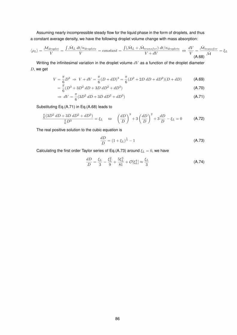
Assuming nearly incompressible steady flow for the liquid phase in the form of droplets, and thus
a constant average density, we have the following droplet volume change with mass absorption:
〈ρL〉 =Mdroplet
V=∫ML dt/ndroplets
V= constant =
∫(ML + Mtransfer) dt/ndroplets
V + dV⇔ dV
V=Mtransfer
M= ξL
(A.68)
Writing the infinitesimal variation in the droplet volume dV as a function of the droplet diameter
D, we get
V =π
6D3 ⇒ V + dV =
π
6(D + dD)3 =
π
6(D2 + 2D dD + dD2)(D + dD) (A.69)
=π
6(D3 + 3D2 dD + 3D dD2 + dD3) (A.70)
⇒ dV =π
6(3D2 dD + 3D dD2 + dD3) (A.71)
Substituting Eq.(A.71) in Eq.(A.68) leads to
π6 (3D2 dD + 3D dD2 + dD3)
π6D
3= ξL ⇔
(dD
D
)3
+ 3(dD
D
)2
+ 3dD
D− ξL = 0 (A.72)
The real positive solution to the cubic equation is
dD
D= (1 + ξL)
13 − 1 (A.73)
Calculating the first order Taylor series of Eq.(A.73) around ξL = 0, we have
dD
D=ξL3− ξ2L
9+
5ξ3L81
+O[ξ4L] ≈ ξL3
(A.74)
86
Appendix B
Simulation Program Formatted Code
87
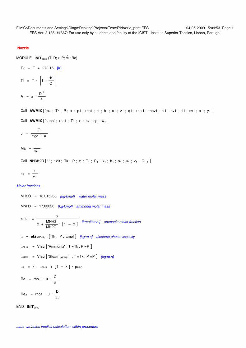
File:C:\Documents and Settings\Dingo\Desktop\Projecto\Tese\F\Nozzle_print.EES 04-05-2009 15:09:53 Page 1
EES Ver. 8.186: #1667: For use only by students and faculty at the ICIST - Instituto Superior Tecnico, Lisbon, Portugal
Nozzle
MODULE INITcond (T; D; x; P; m : Re)
Tk = T + 273,15 [K]
Tl = T · 1 · ·K
C
A = π · D
2
4
Call AWMIX 'tpz' ; Tk ; P ; x : p1 ; rho1 ; t1 ; h1 ; s1 ; z1 ; q1 ; rhol1 ; rhov1 ; hl1 ; hv1 ; sl1 ; sv1 ; x1 ; y1
Call AWMIX 'suppl' ; rho1 ; Tk ; x : cv ; cp ; w1
u = m
rho1 · A
Ma = u
w1
Call NH3H2O ' ' ; 123 ; Tk ; P ; x : T1 ; P1 ; x1 ; h1 ; s1 ; u1 ; v1 ; Qu1
ρ1 = 1
v1
Molar fractions
MH2O = 18,015268 [kg/kmol] water molar mass
MNH3 = 17,03026 [kg/kmol] ammonia molar mass
xmol = x
x + MNH3
MH2O · 1 – x
[kmol/kmol] ammonia molar fraction
µ = etaNH3sliq Tk ; P ; xmol [kg/m.s] disperse phase viscosity
µNH3 = Visc 'Ammonia' ; T =Tk ; P =P
µH2O = Visc 'Steam IAPWS' ; T =Tk ; P =P [kg/m.s]
µ2 = x · µNH3 + 1 – x · µH2O
Re = rho1 · u · D
µ
Re2 = rho1 · u · D
µ2
END INITcond
state variables implicit calculation within procedure
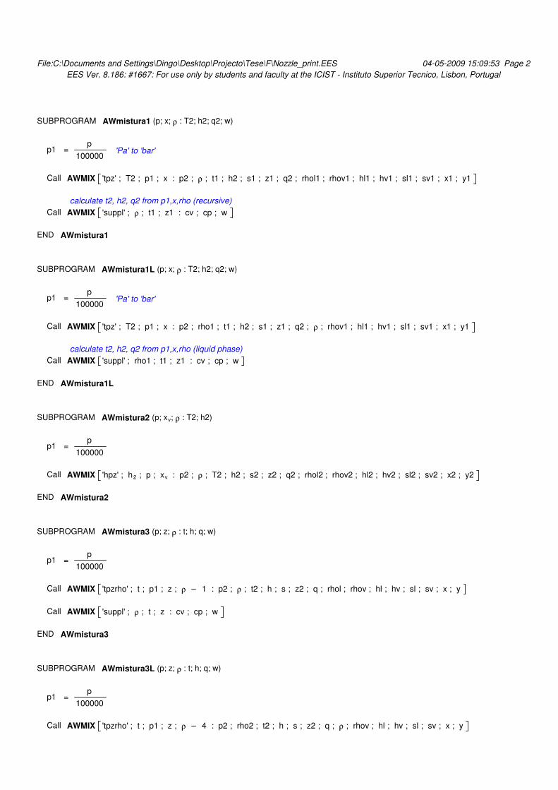
File:C:\Documents and Settings\Dingo\Desktop\Projecto\Tese\F\Nozzle_print.EES 04-05-2009 15:09:53 Page 2
EES Ver. 8.186: #1667: For use only by students and faculty at the ICIST - Instituto Superior Tecnico, Lisbon, Portugal
SUBPROGRAM AWmistura1 (p; x; ρ : T2; h2; q2; w)
p1 = p
100000 'Pa' to 'bar'
Call AWMIX 'tpz' ; T2 ; p1 ; x : p2 ; ρ ; t1 ; h2 ; s1 ; z1 ; q2 ; rhol1 ; rhov1 ; hl1 ; hv1 ; sl1 ; sv1 ; x1 ; y1
calculate t2, h2, q2 from p1,x,rho (recursive)
Call AWMIX 'suppl' ; ρ ; t1 ; z1 : cv ; cp ; w
END AWmistura1
SUBPROGRAM AWmistura1L (p; x; ρ : T2; h2; q2; w)
p1 = p
100000 'Pa' to 'bar'
Call AWMIX 'tpz' ; T2 ; p1 ; x : p2 ; rho1 ; t1 ; h2 ; s1 ; z1 ; q2 ; ρ ; rhov1 ; hl1 ; hv1 ; sl1 ; sv1 ; x1 ; y1
calculate t2, h2, q2 from p1,x,rho (liquid phase)
Call AWMIX 'suppl' ; rho1 ; t1 ; z1 : cv ; cp ; w
END AWmistura1L
SUBPROGRAM AWmistura2 (p; xv; ρ : T2; h2)
p1 = p
100000
Call AWMIX 'hpz' ; h2 ; p ; xv : p2 ; ρ ; T2 ; h2 ; s2 ; z2 ; q2 ; rhol2 ; rhov2 ; hl2 ; hv2 ; sl2 ; sv2 ; x2 ; y2
END AWmistura2
SUBPROGRAM AWmistura3 (p; z; ρ : t; h; q; w)
p1 = p
100000
Call AWMIX 'tpzrho' ; t ; p1 ; z ; ρ – 1 : p2 ; ρ ; t2 ; h ; s ; z2 ; q ; rhol ; rhov ; hl ; hv ; sl ; sv ; x ; y
Call AWMIX 'suppl' ; ρ ; t ; z : cv ; cp ; w
END AWmistura3
SUBPROGRAM AWmistura3L (p; z; ρ : t; h; q; w)
p1 = p
100000
Call AWMIX 'tpzrho' ; t ; p1 ; z ; ρ – 4 : p2 ; rho2 ; t2 ; h ; s ; z2 ; q ; ρ ; rhov ; hl ; hv ; sl ; sv ; x ; y
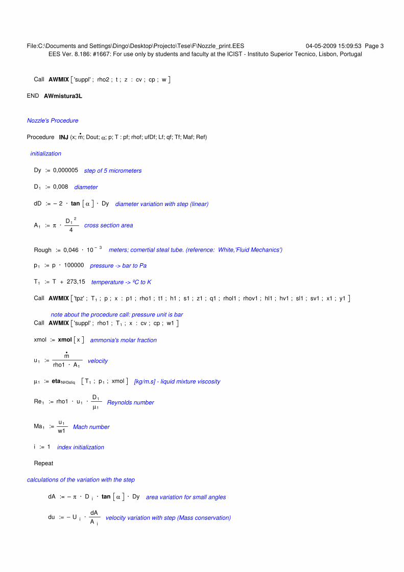
File:C:\Documents and Settings\Dingo\Desktop\Projecto\Tese\F\Nozzle_print.EES 04-05-2009 15:09:53 Page 3
EES Ver. 8.186: #1667: For use only by students and faculty at the ICIST - Instituto Superior Tecnico, Lisbon, Portugal
Call AWMIX 'suppl' ; rho2 ; t ; z : cv ; cp ; w
END AWmistura3L
Nozzle's Procedure
Procedure INJ (x; m; Dout; α; p; T : pf; rhof; ufDf; Lf; qf; Tf; Maf; Ref)
initialization
Dy := 0,000005 step of 5 micrometers
D1 := 0,008 diameter
dD := – 2 · tan α · Dy diameter variation with step (linear)
A1 := π · D1
2
4cross section area
Rough := 0,046 · 10– 3
meters; comertial steal tube. (reference: White,'Fluid Mechanics')
p1 := p · 100000 pressure -> bar to Pa
T1 := T + 273,15 temperature -> ºC to K
Call AWMIX 'tpz' ; T1 ; p ; x : p1 ; rho1 ; t1 ; h1 ; s1 ; z1 ; q1 ; rhol1 ; rhov1 ; hl1 ; hv1 ; sl1 ; sv1 ; x1 ; y1
note about the procedure call: pressure unit is bar
Call AWMIX 'suppl' ; rho1 ; T1 ; x : cv ; cp ; w1
xmol := xmol x ammonia's molar fraction
u1 := m
rho1 · A1
velocity
µ1 := etaNH3sliq T1 ; p1 ; xmol [kg/m.s] - liquid mixture viscosity
Re1 := rho1 · u1 · D1
µ1Reynolds number
Ma1 := u1
w1Mach number
i := 1 index initialization
Repeat
calculations of the variation with the step
dA := – π · D i · tan α · Dy area variation for small angles
du := – U i · dA
A i
velocity variation with step (Mass conservation)
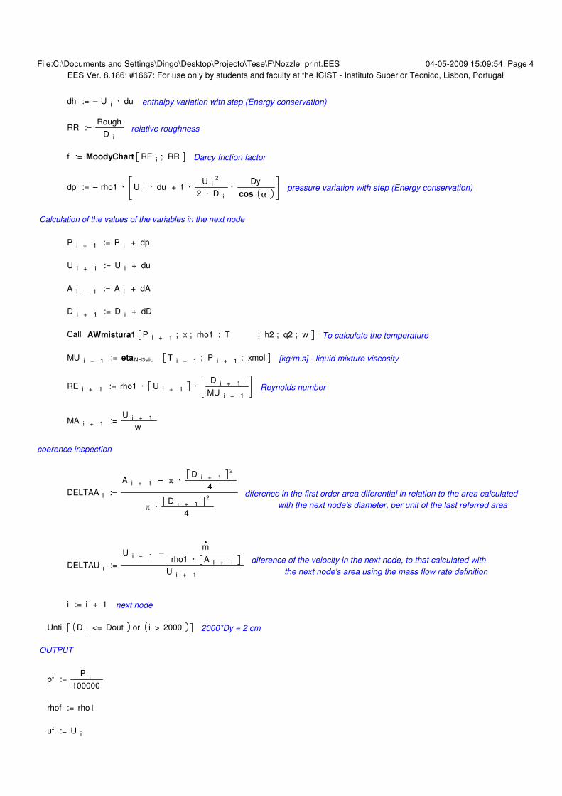
File:C:\Documents and Settings\Dingo\Desktop\Projecto\Tese\F\Nozzle_print.EES 04-05-2009 15:09:54 Page 4
EES Ver. 8.186: #1667: For use only by students and faculty at the ICIST - Instituto Superior Tecnico, Lisbon, Portugal
dh := – U i · du enthalpy variation with step (Energy conservation)
RR := Rough
D i
relative roughness
f := MoodyChart RE i ; RR Darcy friction factor
dp := – rho1 · U i · du + f · U i
2
2 · D i
· Dy
cos αpressure variation with step (Energy conservation)
Calculation of the values of the variables in the next node
P i + 1 := P i + dp
U i + 1 := U i + du
A i + 1 := A i + dA
D i + 1 := D i + dD
Call AWmistura1 P i + 1 ; x ; rho1 : T ; h2 ; q2 ; w To calculate the temperature
MU i + 1 := etaNH3sliq T i + 1 ; P i + 1 ; xmol [kg/m.s] - liquid mixture viscosity
RE i + 1 := rho1 · U i + 1 · D i + 1
MU i + 1
Reynolds number
MA i + 1 := U i + 1
w
coerence inspection
DELTAA i :=
A i + 1 – π · D i + 1
2
4
π · D i + 1
2
4
diference in the first order area diferential in relation to the area calculated
with the next node's diameter, per unit of the last referred area
DELTAU i :=
U i + 1 – m
rho1 · A i + 1
U i + 1
diference of the velocity in the next node, to that calculated with
the next node's area using the mass flow rate definition
i := i + 1 next node
Until D i <= Dout or i > 2000 2000*Dy = 2 cm
OUTPUT
pf := P i
100000
rhof := rho1
uf := U i
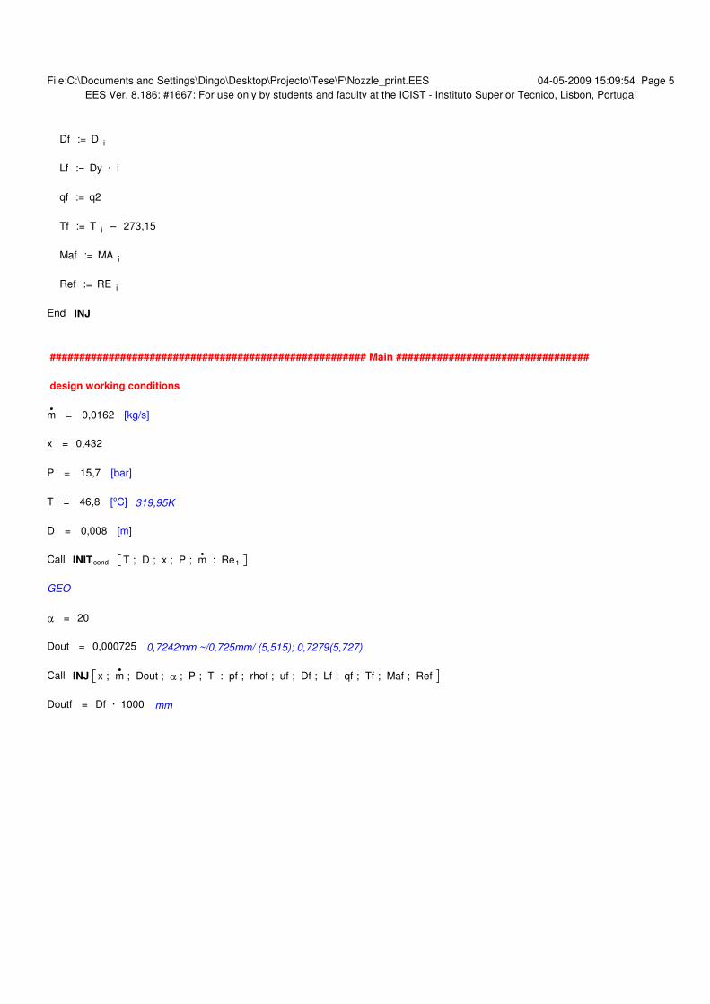
File:C:\Documents and Settings\Dingo\Desktop\Projecto\Tese\F\Nozzle_print.EES 04-05-2009 15:09:54 Page 5
EES Ver. 8.186: #1667: For use only by students and faculty at the ICIST - Instituto Superior Tecnico, Lisbon, Portugal
Df := D i
Lf := Dy · i
qf := q2
Tf := T i – 273,15
Maf := MA i
Ref := RE i
End INJ
###################################################### Main #################################
design working conditions
m = 0,0162 [kg/s]
x = 0,432
P = 15,7 [bar]
T = 46,8 [ºC] 319,95K
D = 0,008 [m]
Call INITcond T ; D ; x ; P ; m : Re1
GEO
α = 20
Dout = 0,000725 0,7242mm ~/0,725mm/ (5,515); 0,7279(5,727)
Call INJ x ; m ; Dout ; α ; P ; T : pf ; rhof ; uf ; Df ; Lf ; qf ; Tf ; Maf ; Ref
Doutf = Df · 1000 mm
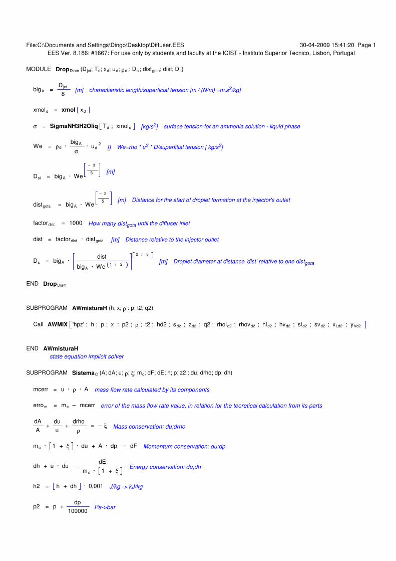
File:C:\Documents and Settings\Dingo\Desktop\Diffuser.EES 30-04-2009 15:41:20 Page 1
EES Ver. 8.186: #1667: For use only by students and faculty at the ICIST - Instituto Superior Tecnico, Lisbon, Portugal
MODULE DropDiam (D jet; Td; xd; ud; ρd : Dsi; distgota; dist; Ds)
bigA = D jet
8[m] charactieristic length/superficial tension [m / (N/m) =m.s2/kg]
xmold = xmol xd
σ = SigmaNH3H2Oliq Td ; xmold [kg/s2] surface tension for an ammonia solution - liquid phase
We = ρd · bigA
σ · ud
2[] We=rho * u2 * D/superfitial tension [ kg/s2]
Dsi = bigA · We
– 3
5 [m]
distgota = bigA · We
– 2
5 [m] Distance for the start of droplet formation at the injector's outlet
factordist = 1000 How many distgota until the diffuser inlet
dist = factordist · distgota [m] Distance relative to the injector outlet
Ds = bigA · dist
bigA · We1 / 2
2 / 3
[m] Droplet diameter at distance 'dist' relative to one distgota
END DropDiam
SUBPROGRAM AWmisturaH (h; x; ρ : p; t2; q2)
Call AWMIX 'hpz' ; h ; p ; x : p2 ; ρ ; t2 ; hd2 ; sd2 ; zd2 ; q2 ; rhold2 ; rhovd2 ; hld2 ; hvd2 ; sld2 ; svd2 ; xLd2 ; yVd2
state equation implicit solver
END AWmisturaH
SUBPROGRAM SistemaC (A; dA; u; ρ; ξ; mc; dF; dE; h; p; z2 : du; drho; dp; dh)
mcerr = u · ρ · A mass flow rate calculated by its components
errom = mc – mcerr error of the mass flow rate value, in relation for the teoretical calculation from its parts
dA
A +
du
u +
drho
ρ = – ξ Mass conservation: du;drho
mc · 1 + ξ · du + A · dp = dF Momentum conservation: du;dp
dh + u · du = dE
mc · 1 + ξEnergy conservation: du;dh
h2 = h + dh · 0,001 J/kg -> kJ/kg
p2 = p + dp
100000Pa->bar
File:C:\Documents and Settings\Dingo\Desktop\Diffuser.EES 30-04-2009 15:41:21 Page 2
EES Ver. 8.186: #1667: For use only by students and faculty at the ICIST - Instituto Superior Tecnico, Lisbon, Portugal
rho2 = ρ + drho
Call AWMIX 'hpz' ; h2 ; p2 ; z2 : p3 ; rho2 ; t3 ; h3 ; s3 ; z3 ; q3 ; rhol3 ; rhov3 ; hl3 ; hv3 ; sl3 ; sv3 ; x3 ; y3
State equations
END SistemaC
Procedure DiffuserC (dy; D; α; Ddroplet; εd; nv; p; mc; md; xc; xd; Tc; Td; uc; ud; index : pf; L; rhocfDf; ucf; Tcf; udf; Tdf; dm; Fperc;
Ftauperc; Ewperc; EQperc; Emperc; Fgota; Ffrica; Qgota; Wfrica; Emass)
---------------------Inicialização das variáveis-------------------------------------------
i := 0 index
L := 0 m lenght
Rough := 0,046 · 10– 3
m for a commertial steal tube (reference: White,'Fluid Mechanics')
A := π · D
2
4[m2] initial diffuser cross section
Ac := A · 1 – εd
dD := 2 · tan α · dy Diffuser Diameter Variation
Vdif := Vcv dy ; D ; α initial elemental volume of the diffuser
Adif := Acv dy ; D ; α initial elemental surface area of the diffuser
N := nv · Vdif [#gota] # of droplets in the first infinitesimal control volume
Vdroplet := π
6 · Ddroplet
3m3 droplet volume
εd2 := Vdroplet · nv Volume fraction of the disperse phase, calculated by the integration of the droplet volume for all droplets
per total volume
errorepsilon := εd – εd2 Volume fraction error, of the input volume fraction in relation to the volume fraction calculated
as above
convertion to Molar Fractions
MH2O := 18,015268 [kg/kmol] Molar Mass - water
MNH3 := 17,03026 [kg/kmol] Molar Mass - ammonia
xmold := xd
xd + MNH3
MH2O · 1 – xd
[kmol/kmol] Molar fraction of ammonia - D phase
xmolc := xc
xc + MNH3
MH2O · 1 – xc
[kmol/kmol] Molar fraction of ammonia - C phase
Initial State variables
File:C:\Documents and Settings\Dingo\Desktop\Diffuser.EES 30-04-2009 15:41:21 Page 3
EES Ver. 8.186: #1667: For use only by students and faculty at the ICIST - Instituto Superior Tecnico, Lisbon, Portugal
Td := Td + 273,15 [K]
Call AWMIX 'tpz' ; Td ; p ; xd : pd ; ρd ; tdD ; hd ; sd ; zd ; qd ; rhold ; rhovd ; hld ; hvd ; sld ; svd ; xLd ; yVd
Call AWMIX 'suppl' ; ρd ; Td ; xd : cvd ; cpd ; wd
Tdi := Td
ρdi := ρd
Tc := Tc + 273,15 [K]
Call AWMIX 'tpz' ; Tc ; p ; xc : pc ; ρc ; tcc ; hc ; sc ; zc ; qc ; rholc ; rhovc ; hlc ; hvc ; slc ; svc ; xLc ; yVc
Call AWMIX 'suppl' ; ρc ; Tc ; xc : cvc ; cpc ; wc
Tci := Tc
ρci := ρc
cpc := 1000 · cpc [J/kg] kJ/kg.K -> J/kg.K
Initial energies, enthalpy: kJ->J
hd := 1000 · hd [J/kg]
ed := hd + ud
2
2[J/kg]
hc := 1000 · hc [J/kg]
ec := hc + uc
2
2[J/kg]
Viscosidade
µc := Visc 'Ammonia' ; T =Tc ; P =p [kg/m.s] Viscosity - C phase (pure ammonia approximation)
µd := etaNH3sliq Td ; p ; xmold [kg/m.s] Viscosity - D phase
νc := µc
ρc
[m2/s] Kinemativ viscosity - C
νd := µd
ρd
[m2/s] Kinematic viscosity - D
Velocidade Relativa
w := ud – uc [m/s] phase relative velocity
dwdy := 0 phase relative velocity rate of variation to length
nº Adimensionais
File:C:\Documents and Settings\Dingo\Desktop\Diffuser.EES 30-04-2009 15:41:21 Page 4
EES Ver. 8.186: #1667: For use only by students and faculty at the ICIST - Instituto Superior Tecnico, Lisbon, Portugal
Mac := uc
wc
Mach number
Mad := ud
wd
Rec := uc · D
νcReynolds number
Red := ud · D
νd
Regota := w · Ddroplet
νcReynolds for the droplet
Quality := ρd · εd
ρd · εd + ρc · 1 – εd
Phase Mixture Quality
################################ CICLO ####################################
Repeat
dA := π · D · tan α · dy Area variation
---------Transfered Quantities---------------
Fd := FD Ddroplet ; w ; ρc ; µc [N] Drag Force on one Droplet (negative for the droplet)
Added Mass, Jelinek et al. correlation
Fdmass := Fmass Ddroplet ; w ; ud ; dwdy ; ρc ; εd Added Mass felt by a Droplet
Difference between correlations
Fdtotal := N · Fd – Fdmass [N] Total force felt by the Disperse Phase
Difusao := DiffusivityNH3 Td ; p ; xmold m/s Diffusivity
Sc := νc
DifusaoSchmidt number for the droplet
dmdrop := Mdropdot Regota ; Sc ; µc ; µd ; xc ; xd ; Difusao ; Ddroplet ; ρc [kg/s] Mass transfered per droplet
dm := N · dmdrop [kg/s] Total mass transfered
mass absorption
Ad := md
ρd · ud
equivalent cross-section area for the disperse phase
mass absorption, Jelinek et al., original correlation
mass absorption, Jelinek et al., correlation used in their study
difference on the two correlations
File:C:\Documents and Settings\Dingo\Desktop\Diffuser.EES 30-04-2009 15:41:21 Page 5
EES Ver. 8.186: #1667: For use only by students and faculty at the ICIST - Instituto Superior Tecnico, Lisbon, Portugal
total
sum of the mass transfer: dmabs->droplet; dme<-droplet (evaporation)
per droplet
kc := KNH3vap Tc [W/m.K] Condutivity - C Phase
Pr := cpc · µc
kc
Prandtl number for the droplet
Qgota := Qdropdot Regota ; Pr ; µc ; µd ; Tc ; Td ; kc ; Ddroplet [W] Heat received by the droplet
dQ := N · Qgota [W] Integrated for all droplets in the element volume
---------Mass Conservation - Quantities----------
ξc := dm
mc
propotion of mass transfered
ξd := dm
md
Massc := mc · 1 – ξc [kg/s] Apparent mass flow rate
Massd := md · 1 + ξd [kg/s] Apparent mass flow rate
dvdroplet1 := dy · dmdrop
ud · ρdm3 droplet volume variation
dDdroplet1 := 2 · dvdroplet1
π · D2 m droplet diameter variation
---------Conservation of NH3 - Ammonia mass fractions----------
dxc := xc – 1
Massc
· dm ammonia's mass fraction variation
dxd := 1 – xd
Massd
· dm
----------Forces on the fluids-------------------------------------------------------------------------------------
Friction
RR := Rough
DRelative Roughness
f := MoodyChart Rec ; RR Darcy friction factor
τ := f · ρc · uc
2
8[Pa] kg/m.s2
File:C:\Documents and Settings\Dingo\Desktop\Diffuser.EES 30-04-2009 15:41:21 Page 6
EES Ver. 8.186: #1667: For use only by students and faculty at the ICIST - Instituto Superior Tecnico, Lisbon, Portugal
dFdy tau := – τ · π · D [N] friction force per unit of lenght
F tau := dFdy tau · dy [N] friction force per elemental volume
Inercc := uc · dm [N] Inertia lost with mass transfer
Inercd := ud · dmdrop [N] Inertia due to mass transfered per droplet
F total;c := F tau – Fdtotal + Inercc [N] Total pressure force
F totaldrop;d := Fd – Inercd [N] Total pressure force - D phase
info quantities
Fperc := – Fdtotal
– F tau – Fdtotal + Inercc
· 100 weight of the drag force on the total force
Ftauperc := – F tau
– F tau – Fdtotal + Inercc
· 100 weight of the friction force on the total force
Fgota := – Fdtotal total drag felt per droplet
Ffrica := – F tau friction felt by the vapour
Aceleracao := Inercc – Fdtotal [N] Total acceleration force felt by the vapour
----------Transfered Power--------------------------------------------------------------------------------------------
dW d := ud · Fd [W] rate of work by the drag force per droplet
dEmd := ed · dmdrop [W] rate of energy variation due to mass transfer per droplet
dE totaldrop;d := Qgota + dW d + dEmd [W] total power transfered per droplet
dE total;d := dE totaldrop;d · N [W] total power transfered for all droplets in the element volume
dW c := uc · – Fdtotal + F tau [W] rate of work by the drag and friction forces
dEmc := – ec · dm [W] rate of energy variation due to mass transfer
dE total;c := – dQ + dW c + dEmc [W] total power transfered for the C phase
info quantities
Ewperc := dW c
– dQ + dW c – dEmc
· 100 weight of work due to friction forces over the total energy transfer
EQperc := – dQ
– dQ + dW c – dEmc
· 100 weight of heat over the total energy transfer
Emperc := – dEmc
– dQ + dW c – dEmc
· 100 weight of work due to mass transfer over the total energy transfer
Qgota := – dQ rate of heat transfer
Wfrica := dW c rate of work due to viscous forces
File:C:\Documents and Settings\Dingo\Desktop\Diffuser.EES 30-04-2009 15:41:21 Page 7
EES Ver. 8.186: #1667: For use only by students and faculty at the ICIST - Instituto Superior Tecnico, Lisbon, Portugal
Emass := – dEmc rate of energy variation due to mass transfer
---------Some Final Quantities --------------------
md2 := md + dm
mc2 := mc – dm
xd2 := xd + dxd
xc2 := xc + dxc
---------------Continuous Phase equation system and solution-------------------------------
Call SistemaC A ; dA ; uc ; ρc ; ξc ; mc ; F total;c ; dE total;c ; hc ; p ; xc2 : duc ; drhoc ; dp ; dhc
hc2 := hc + dhc
uc2 := uc + duc
ρc2 := ρc + drhoc
p2 := p + dp
100000
A2 := A + dA
mc;cal2 := ρc2 · uc2 · A2 element outlet mass flow rate calculated by the product of its parts
erromc := mc – mc;cal2 mass flow rate difference from the obtained by mass conservation directly
Call AWMIX 'hpz' ; hc2 · 0,001 ; p2 ; xc2 : p3 ; rho3 ; t3 ; h3 ; s3 ; z3 ; q3 ; rhol3 ; rhov3 ; hl3 ; hv3 ; sl3 ; sv3
; x3 ; y3
Call AWMIX 'suppl' ; ρc2 ; t3 ; xc2 : cvc2 ; cpc2 ; wc2
erro rhoc := ρc2 – rho3 density error from the obtained by the conservation equations
Tc := t3
----------------Disperse Phase equation system and solutions------------------------
dud := F totaldrop;d · dy
ρd · Vdroplet · ud
[m/s]
dhd := dE total;d
Massd
– ud · dud [J/kg]
ud2 := ud + dud
hd2 := hd + dhd
Call AWMIX 'hpz' ; hd2 · 0,001 ; p2 ; xd : p4 ; rho4 ; t4 ; h4 ; s4 ; z4 ; q4 ; rhol4 ; rhov4 ; hl4 ; hv4 ; sl4 ; sv4
; x4 ; y4
File:C:\Documents and Settings\Dingo\Desktop\Diffuser.EES 30-04-2009 15:41:21 Page 8
EES Ver. 8.186: #1667: For use only by students and faculty at the ICIST - Instituto Superior Tecnico, Lisbon, Portugal
erro rhod := ρd – rho4 error of the density related with the assumption of incompressibility
Td := t4
mcald1 := rho4 · ud2 · εd · A2 element outlet mass flow rate calculated by the product of its parts
erro1md := md2 – mcald1 mass flow rate difference from the obtained by mass conservation directly
mcald2 := ρd · ud2 · εd · A2 element outlet mass flow rate calculated by the product of its parts
erro2md := md2 – mcald2 mass flow rate difference from the obtained by mass conservation directly
Final quantities
p := p2
A := A2
D := D + dD
ρc := ρc2
hc := hc2
uc := uc2
xc := xc2
ud := ud2
hd := hd2
xd := xd2
xmold := xmol xd
Droplet diameter variation
dDdroplet := Ddroplet · ξd
3
Ddroplet := Ddroplet + dDdroplet
cpc := 1000 · cpc2 [J/kg] kJ/... -> J/kg.K
initial energies
ed := hd + ud
2
2[J/kg]
ec := hc + uc
2
2[J/kg]
Viscosity
File:C:\Documents and Settings\Dingo\Desktop\Diffuser.EES 30-04-2009 15:41:21 Page 9
EES Ver. 8.186: #1667: For use only by students and faculty at the ICIST - Instituto Superior Tecnico, Lisbon, Portugal
µc := Visc 'Ammonia' ; T =Tc ; P =p [kg/m.s] Viscosity - C phase
µd := etaNH3sliq Td ; p ; xmold [kg/m.s] Viscosity - D phase
νc := µc
ρc
[m2/s] Kinematic viscosity
νd := µd
ρd
[m2/s]
Relative Velocity
w2 := ud – uc relative phase velocity
dwdy := w2 – w
dyrelative phase velocity variation with length
w := ud – uc [m/s] relative phase velocity
Adimentional quantities
Mac := uc
wc
Mach number
Mad := ud
wd
Rec := uc · D
νcReynolds number
Red := ud · D
νd
Regota := w · Ddroplet
νcReynolds for the droplet
Quality := ρd · εd
ρd · εd + ρc · 1 – εd
Quality of the phase mixture
-------------------change iteration-------------------------
i := i + 1
L := dy · i length
printing to file
F$ := 'C:\d2000am2Fm.csv'
Print F$ ; ; i ; p ; D ; L ; N ; uc ; ud ; Tc ; Td ; mc ; md ; dm ; Fperc ; Ftauperc ; Ewperc ; EQperc ; Emperc ; Fgota ; Ffrica ; Qgota ; W
Quality
Until i >= index
Output quantities
File:C:\Documents and Settings\Dingo\Desktop\Diffuser.EES 30-04-2009 15:41:21 Page 10
EES Ver. 8.186: #1667: For use only by students and faculty at the ICIST - Instituto Superior Tecnico, Lisbon, Portugal
pf := p
Af := A
Df := D
ucf := uc
rhocf := ρc
Tcf := Tc
udf := ud
Tdf := Td
δTc := Tc – Tci
δTd := Td – Tdi
End DiffuserC
############################################################## END OF PROCEDURE ##########################
#####################
>>>>>>>>>>>>>>>>>>>>>>>>>>>>>>>>>>>>>>>>>>>>>> Main <<<<<<<<<<<<<<<<<<<<<<<<<<<<<<<<<<<<<<<<<<<<<<<<<<<<<<
<<<<<<<<<<<<<<<<<<<<<<<<<<<<<<<<<<<<<<<<<<<<<<<<<<
..........................................................................................................Initial parameters.................................................................................
..................................
p = 5,515 [bar]
Disperse phase - poor solution
md = 0,0162 [kg/s]
xd = 0,432
Td = 46,35 [C]
Td = Td + 273,15 [K]
Call AWMIX 'tpz' ; Td ; p ; xd : pd ; ρd ; tdD ; hd ; sd ; zd ; qd ; rhold ; rhovd ; hld ; hvd ; sld ; svd ; xLd ; yVd
Call AWMIX 'suppl' ; ρd ; Td ; xd : cvd ; cpd ; wd
ud = 49,07 [m/s]
md = ρd · ud · Ad
Ad = π · Dd
2
4
File:C:\Documents and Settings\Dingo\Desktop\Diffuser.EES 30-04-2009 15:41:21 Page 11
EES Ver. 8.186: #1667: For use only by students and faculty at the ICIST - Instituto Superior Tecnico, Lisbon, Portugal
D jet = 0,0007242 [m]
Dd – D jet = δDd
Continuous phase - vapour
mc = 0,00267 [kg/s]
xc = 0,985
Tc = 34,4 [C]
Tc = Tc + 273,15 [K]
Call AWMIX 'tpz' ; Tc ; p ; xc : pc ; ρc ; tcc ; hc ; sc ; zc ; qc ; rholc ; rhovc ; hlc ; hvc ; slc ; svc ; xLc ; yVc
Call AWMIX 'suppl' ; ρc ; Tc ; xc : cvc ; cpc ; wc
Dc = 0,01 [m]
Ac = π · Dc
2
4
mc = ρc · uc · Ac
ρcpuro = ρ 'Ammonia' ; T =Tc ; P =p · 100000 Ammonia's density in the same conditions as the affected mixture
Geometrical
dy = 0,0005 [m] 500 micrometers length between nodes
[Degrees]
Diffuser's angle
..........................................................................................................Calculation of other parameters....................................................................
.....................................
A = Ac + Ad diffuser inlet area
A = π · D
2
4diffuser inlet diameter
inicial mass flow rate of the multi-phase mixture entering the diffuser - mean-phase content calculation
εd · ρd · ud · A = md discrete phase
1 – εd2 · ρc · uc · A = mc continuous phase
δε = εd – εd2 error in the volume fraction calculation
Quality = ρd · εd
ρd · εd + ρc · 1 – εd
Quality for the phases mixture
Nr of droplets:
File:C:\Documents and Settings\Dingo\Desktop\Diffuser.EES 30-04-2009 15:41:21 Page 12
EES Ver. 8.186: #1667: For use only by students and faculty at the ICIST - Instituto Superior Tecnico, Lisbon, Portugal
Call DropDiam D jet ; Td ; xd ; ud ; ρd : Dsi ; dropletdist ; dist ; Ds
Ddroplet = Ds [m] Initial mean droplet diameter
vgota = π
6 · Ddroplet
3[m3] droplet mean initial volume
nv temp = εd
vgota
[1/m3]
nv = Round nv temp [#/m3] droplet density / # droplets per volume unit, rounded to an integer
V = Vcv dy ; D ; α initial control volume
N = nv · V # droplets inside the initial control volume, for reference
Diffuser
Call DiffuserC dy ; D ; α ; Ddroplet ; εd ; nv ; p ; mc ; md ; xc ; xd ; Tc ; Td ; uc ; ud ; index : pf ; L ; rhocf ; Df ; ucf
; Tcf ; udf ; Tdf ; dm ; Fperc ; Ftauperc ; Ewperc ; EQperc ; Emperc ; Fgota ; Ffrica ; Qgota ; Wfrica ; Emass
δP = pf – p
Tcf = Tcf – 273,15
Tdf = Tdf – 273,15
δTc = Tcf – Tc
δTd = Tdf – Td
δuf = udf – ucf
drhoc = rhocf – ρc
File:C:\EES32\Userlib\droplet_dynamics\Transferquanties.LIB 02-05-2009 12:18:35 Page 1
EES Ver. 8.186: #1667: For use only by students and faculty at the ICIST - Instituto Superior Tecnico, Lisbon, Portugal
Funções para o cálculo das quantidades transferidas para uma gota/partícula em movimento
Functions that calculate the quantities transferred for a moving droplet/particle
Function Qdropdot (Re; Pr; µC; µD; TC; TD; kC; D)
If Re <= 0 or Pr <= 0 Then
ν := 2
Else
ν := 2 + 0,6 · Re1 / 2
· Pr1 / 3
EndIf
Qdrop := ν · kC · π · D · TC – TD
End Qdropdot
Function Mdropdot (Re; Sc; µC; µD; xC; xD; Difusao; D; ρC)
If Re >= 0 Then
Sh := 2 + 0,6 · Re1 / 2
· Sc1 / 3
Else
Sh := 2 + 0,6 · – Re1 / 2
· Sc1 / 3
EndIf
Mdrop := Sh · Difusao · π · D · ρC · xC – xD
End Mdropdot
Function Mabsobdot (Ad; Ddroplet; ρd; xC; xD; Difusao; ud; dy)
If ud <= 0 Then
Mabsob := 17,66 · ρd · Difusao
Ddroplet
· 6 · Ad
Ddroplet
· xC – xD
Else
td := 1
ud
· dy
Mabsob := 6 · Ad
Ddroplet
· ρd · xD – xC · Difusao
π · td
EndIf
End Mabsobdot
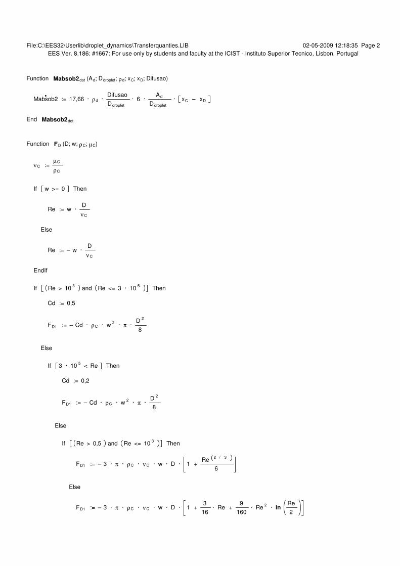
File:C:\EES32\Userlib\droplet_dynamics\Transferquanties.LIB 02-05-2009 12:18:35 Page 2
EES Ver. 8.186: #1667: For use only by students and faculty at the ICIST - Instituto Superior Tecnico, Lisbon, Portugal
Function Mabsob2dot (Ad; Ddroplet; ρd; xC; xD; Difusao)
Mabsob2 := 17,66 · ρd · Difusao
Ddroplet
· 6 · Ad
Ddroplet
· xC – xD
End Mabsob2dot
Function FD (D; w; ρC; µC)
νC := µC
ρC
If w >= 0 Then
Re := w · D
νC
Else
Re := – w · D
νC
EndIf
If Re > 103
and Re <= 3 · 105
Then
Cd := 0,5
FD1 := – Cd · ρC · w2
· π · D
2
8
Else
If 3 · 105
< Re Then
Cd := 0,2
FD1 := – Cd · ρC · w2
· π · D
2
8
Else
If Re > 0,5 and Re <= 103
Then
FD1 := – 3 · π · ρC · νC · w · D · 1 + Re
2 / 3
6
Else
FD1 := – 3 · π · ρC · νC · w · D · 1 + 3
16 · Re +
9
160 · Re
2 · ln
Re
2
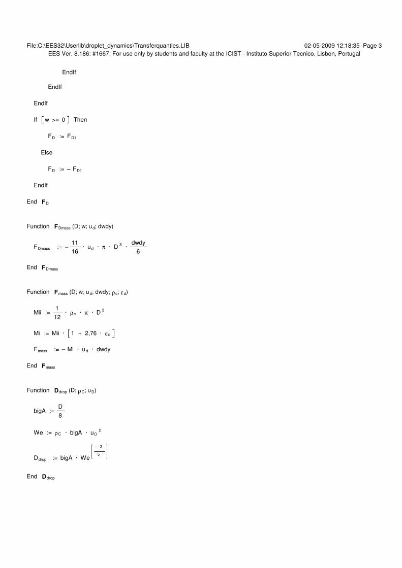
File:C:\EES32\Userlib\droplet_dynamics\Transferquanties.LIB 02-05-2009 12:18:35 Page 3
EES Ver. 8.186: #1667: For use only by students and faculty at the ICIST - Instituto Superior Tecnico, Lisbon, Portugal
EndIf
EndIf
EndIf
If w >= 0 Then
FD := FD1
Else
FD := – FD1
EndIf
End FD
Function FDmass (D; w; ud; dwdy)
FDmass := –11
16 · ud · π · D
3 ·
dwdy
6
End FDmass
Function Fmass (D; w; ud; dwdy; ρc; εd)
Mii := 1
12 · ρc · π · D
3
Mi := Mii · 1 + 2,76 · εd
Fmass := – Mi · ud · dwdy
End Fmass
Function Ddrop (D; ρC; uD)
bigA := D
8
We := ρC · bigA · uD2
Ddrop := bigA · We
– 3
5
End Ddrop